Dis cus si on Paper No. 13-075

Modelling Production Cost Scenarios for Biofuels and

Fossil Fuels in Europe

Gunter Festel, Martin Würmseher, Christian Rammer, Eckhard Boles,

and Martin Bellof

Dis cus si on Paper No. 13-075

Modelling Production Cost Scenarios for Biofuels and

Fossil Fuels in Europe

Gunter Festel, Martin Würmseher, Christian Rammer, Eckhard Boles,

and Martin Bellof

Download this ZEW Discussion Paper from our ftp server:

http://ftp.zew.de/pub/zew-docs/dp/dp13075.pdf

Die Dis cus si on Pape rs die nen einer mög lichst schnel len Ver brei tung von neue ren For schungs arbei ten des ZEW. Die Bei trä ge lie gen in allei ni ger Ver ant wor tung

der Auto ren und stel len nicht not wen di ger wei se die Mei nung des ZEW dar.

Dis cus si on Papers are inten ded to make results of ZEW research prompt ly avai la ble to other eco no mists in order to encou ra ge dis cus si on and sug gesti ons for revi si ons. The aut hors are sole ly

respon si ble for the con tents which do not neces sa ri ly repre sent the opi ni on of the ZEW.

Das Wichtigste in Kürze

Sollen sich Biokraftstoffe im Markt als Ersatz für konventionelle, auf Erdöl basierte Kraftstof-

fe durchsetzen, so sind wettbewerbsfähige Produktionskosten für Biokraftstoffe eine unab-

dingbare Voraussetzung. Denn die derzeit verfolgte steuerliche Förderung von Biokraftstoffen

wird nicht auf Dauer finanziert werden. Ein Vergleich der Wettbewerbsfähigkeit der Produk-

tionskosten für verschiedene Biokraftstoffe ist allerdings nicht einfach, da neben den Markt-

preisen für die eingesetzten Biorohstoffe weitere, sehr unterschiedliche Faktoren die Produk-

tionskosten bestimmen. Das Ziel dieses Beitrags ist es, 1) künftige Preisniveaus für verschie-

dene Biorohstoffe in Abhängigkeit von der Entwicklung der Rohölpreise sowie weiterer Ein-

flussgrößen (u.a. Preis- und Nachfrageentwicklung von Agrarrohstoffen, Entwicklung der

Energienachfrage) zu schätzen, 2) künftige Produktionskosten für verschiedene Biokraftstoff-

arten unter Annahmen über die Nutzung von Skaleneffekten und technologischen Lerneffek-

ten zu simulieren und 3) Produktionskosten für verschiedene Biokraftstoffe am Standort Eu-

ropa mit den Kosten von auf Erdöl basierten Kraftstoffen im Rahmen einer Szenarioanalyse

für die Jahre 2015 und 2020 zu vergleichen.

Als Grundlage für weitere Analysen wird ein Berechnungsmodell für die Biokraftstoffproduk-

tion vorgestellt. Im Gegensatz zu ingenieurwissenschaftlich orientierten Bottom-up-Ansätzen,

die in der Literatur bisher meist verwendet wurden, um Biokraftstoffe aus einer technischen

und zumeist individuellen Perspektive zu untersuchen, wird in diesem Beitrag ein gesamtwirt-

schaftlicher Top-down-Ansatz herangezogen. Dadurch ist es möglich, die Auswirkungen un-

terschiedlicher Rohstoffpreisentwicklungen und die relative Wettbewerbsfähigkeit verschie-

dener Biokraftstoffe untereinander, als auch gegenüber fossilen Kraftstoffen hinsichtlich ihrer

wirtschaftlichen Potentiale zu vergleichen. Dabei kommen vier Szenarien der künftigen Roh-

ölpreisentwicklung bis 2020 (€50, €100, €150 und €200 je Barrel) zum Einsatz.

Die Ergebnisse zeigen, dass Biokraftstoffe der 2. Generation (d.h. die nicht auf Nahrungsmit-

telrohstoffen wie Zuckerrohr, Rapsöl, Palmöl oder Weizen, sondern auf anderen pflanzlichen

Rohstoffen – Holz, pflanzliche Abfälle, Altöl aus pflanzlicher Herkunft) am ehesten mittel-

bis langfristig ein im Vergleich zu Erdöl wettbewerbsfähiges Kostenniveau erreichen können,

und zwar sowohl bei niedrigen (€50) als auch bei hohen (€200) Rohölpreisen. Voraussetzung

ist aber, dass Skalen- und Lerneffekte umfassend genutzt werden. Insbesondere Bioethanol

auf Basis von Lignozellulose und Bio-Diesel auf Basis von pflanzlichem Altöl zeigen im

Vergleich zu Biokraftstoffen der 1. Generation hohe Kosteneinsparungspotenziale.

Executive Summary

Competitive production costs compared to conventional fuels are imperative for biofuels to

gain market shares, as current tax advantages for biofuels are only temporary. Comparing pro-

duction costs of different biofuels with fossil fuels is a challenge due to the complexity of

influencing factors. The objective of this research paper is threefold: 1) to project future bio-

fuel feedstock prices based on the crude oil price development, the price index for agricultural

products, growth in world population, growth in wealth per capita income, and change in en-

ergy consumption per capita, 2) to simulate production costs under consideration of likely

economies of scale from scaling-up production size and technological learning and 3) to com-

pare different biofuels and fossil fuels by scenario analysis.

A calculation model for biofuel production is used to analyse projected production costs for

different types of biofuels in Europe for 2015 and 2020. Unlike engineering oriented bottom-

up approaches that are often used in other biofuel studies, the macro-economic top-down ap-

proach applied in this study enables an economic comparison and discussion of various fuel

types based on reference scenarios of crude oil prices of €50, €100, €150 and €200 per barrel.

Depending on the specific raw material prices as well as the conversion costs, the analysis

delivered a differentiated view on the production costs and thus on the competitiveness of

each individual type of fuel.

The results show that 2nd generation biofuels are most likely to achieve competitive produc-

tion costs mid- to long-term when taking into account the effects from technological learning

and production scale size as well as crude oil price scenarios between €50 and €200 per barrel

for both reference years. In all crude oil price scenarios, bioethanol from lignocellulosic raw

materials as well as biodiesel from waste oil are associated with high cost saving potentials

which enable them to outperform fossil fuels and 1st generation biofuels.

Modelling Production Cost Scenarios for Biofuels and Fossil Fuels in Europe

Gunter Festela,b,c,f*, Martin Würmseherb,c, Christian Rammerd, Eckhard Bolese , Martin Belloff

a Festel Capital, Fuerigen, Switzerland

b Butalco GmbH, Fuerigen, Switzerland c Department of Management, Technology, and Economics, Swiss Federal Institute of Technology Zurich,

Switzerland d Department of Industrial Economics and International Management, Centre for European Economic Research

(ZEW), Mannheim, Germany e Institute of Molecular Biosciences, Goethe-University Frankfurt, Germany

f Autodisplay Biotech GmbH, Düsseldorf, Germany

September 2013

Abstract

This paper presents the results of a calculation model for biofuel production costs in 2015 and 2020 based on raw material price projections and considering scale and learning effects. Distinguishing six types of biofuels, the paper finds that scale economies and learning effects are critical for 2nd generation biofuels to become competitive. In case these effects can be utilized, cost saving potentials for 2nd generation biofuels are significant.

Keywords: Biofuels, Production Cost Scenarios, Raw Material Price Projection, Conver-sion Costs

JEL-Classification: L25, L26, J24 * Corresponding author: Festel Capital, Mettlenstrasse 14, CH-6363 Fuerigen, Switzerland, phone/fax

+41 41 780 1643, email gunter.festel@festel.com

1

1. Introduction

A large portion of worldwide energy sources and tangible products are made from fossil re-

sources. Crude oil is the single most important source of energy accounting for approximately

35% of worldwide primary energy consumption in 2005 and is expected to slightly decrease

to 32% by 2030 (IEA, 2007). Although crude oil, natural gas and coal will still remain the

most important sources of energy until at least 2030 (U.S. EIA, 2011; Birol, 2010), depleting

oil reserves have been recognised as a main challenge to energy supply in the next decades.

Owing to the rising crude oil price and stricter emission standards, the demand for alternative

fuels is growing. Alternative fuels able to mitigate climate change and reduce the consump-

tion of fossil resources are increasingly being promoted by governments (Gustavsson, 1997;

Mizsey and Racz, 2010; Fargione et al., 2008; Balat, 2011). Among these alternative fuels,

biofuels are particularly important to bridge the gap until fuel cell or electrically driven vehi-

cles are available on a large scale. The replacement of oil with biomass as raw material for

fuel and chemical production is an interesting option and a driving force for the development

of so-called biorefineries, where almost all types of biomass feedstocks can be converted to

different products (Cherubini, 2010).

Renewable resources can lead to a higher security of supply and a better environmental per-

formance due to lower greenhouse gas (GHG) emissions (Parry, 1999), and may also increase

income in rural regions (Leistritz and Hodur, 2008). Some authors even expect the develop-

ment of a bio-based economy (Tyner and Taheripour, 2008). Of special interest is the produc-

tion of biofuels, such as bioethanol, biodiesel or biomass-to-liquids (BTL) fuel using various

raw materials and production processes (Naik et al., 2010). In contrast to biofuels of the 1st

generation (bioethanol from sugar or starch containing plants or biodiesel from rape seed or

palm oil), 2nd generation biofuels are made from raw materials which are not used for the

production of food products. These raw materials mainly include lignocellulosic materials (or

lignocellulosic waste), such as straw and wood as well as various agricultural and wood proc-

essing waste products, such as organic waste. Ajanovic (2011) concludes that besides the ad-

vantage related to the absence of competition for raw materials with food production, 2nd

generation biofuels are associated with higher energy yields, modest use of agro-chemicals

and higher reduction potential of greenhouse gas emissions compared to 1st generation biofu-

els. The use of biofuels has increased considerably in the European Union (EU) (Bomb et al.,

2

2007; Dautzenberg and Hantl, 2008), although, so far, only first generation biofuels are being

produced in larger scales.

The main objective of this paper is to calculate biofuel production costs for different biofuels

in Europe for the two years 2015 and 2002 and compare them with production costs for fossil

fuels. For this purpose, a calculation model consisting of four steps was developed: 1) defini-

tion of biofuel production scenarios in 2015 and 2020, 2) estimation of future raw material

prices based on assumptions on crude oil price development and the observed relation be-

tween crude oil price and prices for biofuel raw materials in the past, 3) modelling of scale

and time dependant conversion and capital costs and 4) calculation of the total production

costs as sum of raw material costs, capital costs and conversion costs. The input data for the

production cost model are taken from publicly available production cost data for production

processes as well as single production steps which were collected during the past five years

based on literature research and expert interviews (Festel, 2008; Festel, 2007). The production

costs are calculated in Euro Cent per litre (€Cent/l). The accuracy of the results was enhanced

by plausibility checks based on current data as well as consistency of the results across pro-

duction technologies. Simultaneously, data comparability was assessed in this course and, if

necessary, corresponding adjustments were performed.

Both changes in raw material costs and conversion costs as well as capital costs based on dif-

ferent scenarios of price development for raw materials and crude oil were considered. Raw

material costs are driven by the development of the markets for biomass and fossil raw mate-

rials, like crude oil due to substitution effects. Conversion costs are driven by scale effects as

well as time dependent learning effects. Demand side restrictions in the availability of biofu-

els due to a strongly increasing demand and rapidly raising biofuel prices are assumed as neg-

ligible for this projection period. Despite the peak oil issue, biofuels are not expected to ex-

ceed a market share of 15% on the global fuel market within the next five to ten years (Gnan-

sounou et al., 2009; Bagheri, 2011). The EU has set a target market share of 10% in terms of

all petrol and diesel transport fuels in the EU by 2020 (EU-Commission, 2003). Consequently,

prices on the fuel market will still be driven by fossil fuels.

Today, biofuels can compete with fossil fuels only due to governments’ regulation and subsi-

dies. The hypothesis of this study is that medium and long term biofuel demand will become

decreasingly based on governmental regulations and more and more on cost competiveness

compared to fossil fuels. If biofuels can be produced cheaper than fossil fuels, demand will be

3

high enough during the next years to absorb all the produced biofuel quantities. Therefore,

biofuel production costs will be responsible for the market share of biofuels.

In this model it was assumed that biofuel demand in Europe will be met by biofuel production

in Europe and the option of biofuel production at other locations and import of biofuels was

neglected. European production sites may benefit from a more developed production infra-

structure, economies of scope to other production activities and greater proximity to end users.

The production cost input data are focused on the situation in Europe but the model could

easily be applied to other regions if the input data are changed accordingly.

2. Related Literature

2.1. Calculation models for energy production costs

Various calculation models have been developed to give a better insight into the complexities

of energy production systems under a range of policy objectives. Many authors describe the

entire energy system either through the use of a technical bottom-up approach or a macro-

economic top-down approach (Junginger et al., 2008). There are also a number of studies

evaluating whole supply chains for biobased products (Stephen et al., 2010; Kim et al., 2011),

biorefinery concepts (Fernando et al., 2006; Clark, 2007; Francesco, 2010) or the potential of

biofuels for individual countries (Martinsen et al., 2010). For example, Kim et al. (2011) use a

mixed integer linear programming model that enables the selection of fuel conversion tech-

nologies, capacities, biomass locations, and the logistics of transportation from the raw mate-

rial locations to the conversion sites and then to the final markets.

Furthermore, there are numerous specific evaluations of biofuels, like biodiesel (Zhang et al.,

2003; van Kasteren and Nisworo, 2007; Araujo et al., 2010) and simulations of biofuel proc-

esses with specialised software, like Aspen HYSYS (West et al., 2008). Despite the fact that

production costs of biofuels compared to fossil fuels are an important driver for biofuel de-

mand, there are only a few approaches to compare different biofuel production processes with

each other and with the established production of fossil fuels considering scale and learning

curve effects in the production process. Whereas some studies focus on individual process

steps, like production costs for enzymes (Tufvesson et al., 2011; Klein-Marcuschamer et al.,

2012), other studies compare different biofuels based on a production cost analysis (Bridge-

water and Double, 1994; Giampietro and Ulgiati, 2005; de Wit et al., 2010; NREL, 2011).

The analysis by de Wit et al. (2010), for example, shows that biodiesel is the most cost com-

4

petitive fuel, dominating the early market of 1st generation biofuels. The better cost perform-

ance of biodiesel compared to 1st generation bioethanol can be explained by lower feedstock

costs for oil crops compared to sugar or starch crops together with lower capital and opera-

tional expenses for transesterification of oil to biodiesel compared to the hydrolysis and fer-

mentation of sugar or starch crops to bioethanol (de Wit et. al., 2010).

Feedstock production costs can decrease over time, mainly by scale economies and by gaining

technological experience with its production. Analyses performed for sugarcane in Brazil (van

den Wall Bake et al., 2009), for corn in the US (Hettinga et al., 2009) and for rapeseed in

Germany (Berghout, 2008) demonstrated that indeed cost reductions of (food) crops do fol-

low an experience (or learning) curve pattern. In addition, other research papers investigated

the economic dependency of fossil fuels and the potential replacement of crude oil by biomass

(Dixon et al., 2007). The expanded use of biofuels competes with the energetic use of biomass

in residential applications and heat/power generation in the conversion sector as well as food

production, animal feed and industrial production. So, due to the utilisation of certain feed-

stocks, there are also negative spill over effects from the production of biofuels on global food

prices. Owing to arbitrage effects, the positive correlation between biofuel production scale

and global food prices becomes particularly evident when crude oil prices rise (Chen et al.,

2010). For example, the growth of corn-based ethanol production and soybean-based bio-

diesel production, following the increase in the oil price, has significantly affected the world

agricultural grain productions and its prices. As biomass can also be used as raw material for

chemicals and numerous other applications, biomass prices are not only driven by the fuel

industry (Swinnen and Tollens, 1991; Hermann and Patel, 2006).

2.2. Scale and learning effects on production costs

The combination of economies of scale and cost reductions through technological learning is

an essential element for the analysis of production costs (de Wit et al., 2010). A concept to

measure and quantify the aggregated effect of technological learning is the experience curve

approach. This commonly used approach states that costs decline with a fixed percentage

amount over each doubling in cumulative production (Hettinga et al., 2009). Although learn-

ing curve effects have increasingly been incorporated in many energy models, only a few au-

thors, like de Wit et al. (2010), specified corresponding models with a particular focus on bio-

fuels. In line with studies on biomass integrated gasification/combined cycle (BIG/CC) plants

for electricity production (Faaij et al., 1998; Uyterlinde et al., 2007), learning curve effects

5

can be considered by estimating progress ratios for distinct process steps of biofuel produc-

tion processes.

For the investigation of production costs, a distinction between two effects on efficiency must

be made, depending on whether their impact on cost projections is driven by the production

scale size (scale effects) or by technological process improvements (learning effects).

Whereas learning effects are dynamic in nature and will accumulate over time (typically with

a decreasing pace), scale effects are static, though they may also have a dynamic component if

production capacities expand over time. Over the past decades, various researchers have at-

tempted to distinguish between static scale economies and dynamic learning effects (Stobaugh

and Townsend, 1975; Sultan, 1975; Hollander, 1965; Preston and Keachie, 1964). In sum-

mary, these studies have discovered static scale effects to be statistically significant but small

in magnitude relative to learning-based effects (Liebermann, 1984).

The scale effect is based on a scale law describing the inverse correlation between increases in

plant scale and the associated decrease in production costs (Blok, 2006; Haldi and Whitcomb,

1967). On the one hand, up to a certain point, larger production scales are associated with

marginal costs per output unit that are increasing but still below the average costs per unit,

which leads to decreasing average costs per unit of biofuel outcome. On the other hand, over-

capacities at any stage along the value chain are to be minimised and transport costs have to

be considered, which leads to an optimal production scale for each production facility. Fur-

thermore, for the determination of the optimum plant size the specific characteristics of each

type of biofuel should be taken into account. Exemplary for bioethanol production, Nguyen

and Prince (1996) showed that through other measures, such as the use of mixed crops to ex-

tend the processing season, the capital costs per unit of bioethanol outcome can be reduced.

Thus, total production costs decrease which, in turn, results in a lower optimum plant size.

Beyond scale-dependant potentials to improve cost efficiency, there are scale-independent

potentials for further cost reductions from technological advancements and other learning

benefits related to the production process. As examples for these scale-independent cost ef-

fects, de Wit et al. (2010) mention more efficient organisation of production and transporta-

tion processes, the use of advanced materials and lifetime prolongation of catalysts. In total,

the significance of the scale-independent learning component becomes evident in various

studies. These demonstrate that the related cost reduction potentials for ethanol production

from corn (Hettinga et al., 2009) and sugarcane (van den Wall Bake et al., 2009; Hamelinck et

al., 2005) range from 25% to 50%.

6

These examples show that, given the complex interactions between fossil fuels and the vari-

ous biofuels, top-down models to easily understand the production costs for fossil fuels and

biofuels without too many technical details can be a useful tool for producers, investors and

policy makers. This paper attempts to contribute to this discussion by developing a simple

top-down calculation model for biofuel production in Europe based on different raw materials

and conversion technologies compared to fossil fuels for the years 2015 and 2020.

3. Types of biofuels

This section describes the different types of biofuels examined in this study and explains the

calculation model to determine production costs.

The analysed biofuels were defined as a combination of raw materials and conversion tech-

nologies following Fig. 1: 1st generation and 2nd generation bioethanol as well as biodiesel,

hydrated vegetable oil (HVO) and BTL fuel.

Fig. 1. Investigated biofuels with standardised production process steps

Raw materialsProcess step 1: Pretreatment

Process step 2: Conversion

Process step 3: Purification

Biofuels

MaizeWheat

Rapeseed oilPalm oil

Palm oil Purification Hydrogenation Destillation HVO

Wood Gasification FT synthesis Reforming/destillation BTL

Purification Transesterification Purification Biodiesel (1st gen)

Waste oil Purification Transesterification Purification Biodiesel (2st gen)

Enzymatic hydrolysis

FermentationDestillation and

molecular sievesEthanol (1st gen)

Waste lignocelluloseEnzymatic hydrolysis

FermentationDestillation and

molecular sievesEthanol (2nd gen)

Bioethanol is produced by the fermentation of sugar and starch containing organic materials.

Whereas sugar containing plants can be directly fermented, starch containing plants have to

first be converted to sugars using enzymes. During the fermentation process microorganisms,

such as yeast, convert sugars into ethanol. Bioethanol yields can be increased significantly

should lignocellulose be processed to bioethanol. In comparison to using sugar and starch

containing raw materials this process is more complex due to the conversion of lignocellulose

to sugar. As yet, no large scale production of bioethanol from lignocellulose exists, although

7

researchers (Kim and Dale, 2004) estimated that lignocellulosic biomass could produce up to

442 billion litres per year of bioethanol.

Biodiesel is won from plant oils (most commonly used is rapeseed oil with an oil content of

40-45%) or animal fats and transesterification with methanol. The largest disadvantage of

biodiesel is that it acts aggressively against some rubbers and plastic, and rubber parts in the

fuel system may corrode in time. It also could clog filters inside the tank or cause leaking

seals. As outlined by Antoni et al. (2007), most diesel cars have been licensed to use a blend

of diesel with biodiesel of up to 5%. In Germany, for example, the conversion of a conven-

tional diesel engine for pure biodiesel use is offered by many companies for up to €1,500 per

car. At the same time, however, the modified engine requires more frequent engine oil

changes.

Like biodiesel, HVO can be produced from oil-containing raw materials. Hydrotreating of

vegetable oils or animal fats is an alternative process to esterification for producing bio-based

diesel fuels (Mikkonen, 2008; Hodge, 2008). The first commercial scale HVO plant with a

capacity of 170 000 tonnes per year was started up in 2007 in Finland. Several HVO units

with a scale of up to 800 000 tonnes per year per unit are under consideration by many oil

companies and process technology suppliers around the world.

The production of BTL fuel comprises of a number of different process steps. First, the bio-

mass is broken down into coke and a gas containing tar by means of a low temperature gasi-

fier. In a gasification reactor, a tar-free synthesis gas is produced which is then liquefied in a

Fischer-Tropsch reaction to fuel. BTL fuels can be used, depending on the octane number, in

conventional petrol or diesel powered cars without requiring any modification to the engine.

Fischer-Tropsch plants for producing BTL fuels from biomass, like wood and residues, are

estimated to be in commercial scale within the next decade.

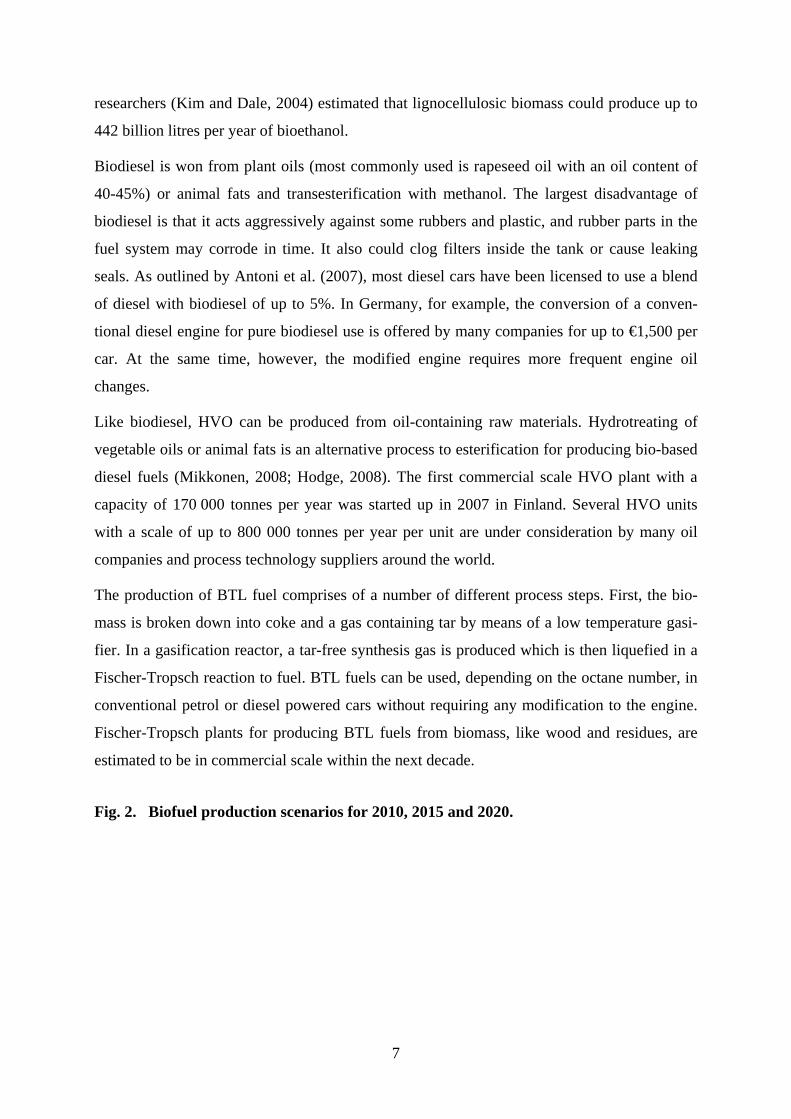
Fig. 2. Biofuel production scenarios for 2010, 2015 and 2020.

8

Demonstration scale

Biofuels Raw materials 2010 2011 2012 2013 2014 2015 2016 2017 2018 2019 2020

Ethanol (1st gen) MaizeEthanol (1st gen) WheatEthanol (2nd gen) Waste lignocelluloseBiodiesel (1st gen) Rapeseed oilBiodiesel (1st gen) Palm oilBiodiesel (2st gen) Waste oilHVO Palm oilBTL Wood

Pilot scale

Production scale

As maturity of the technology has a decisive impact on production costs and some technolo-

gies are not expected to leave pilot or demonstration stage in the foreseeable future, the first

step in the analysis is the projection of the production scale for each technology in the future.

Thus, based on the maturity of each biofuel technology, a comparable reference scenarios

related to biofuel production for the years 2015 (scenario 2015) and 2020 (scenario 2020) (Fig.

2) was defined. For each scenario the (projected) status (pilot scale, demonstration scale or

production scale) of each technology for the corresponding year was compared. Through this

procedure, the analysis takes into account that the more mature technologies have larger

scales than technologies under development, thus more mature technologies offer a significant

cost advantage.

4. Scenarios for future raw material prices

Raw material prices are critical for the economic viability of biofuel production. Profitability

of biofuels depends on prices for biofuel raw materials and the price for crude oil as key com-

petitor product. This section presents the method used to derive scenarios for future develop-

ment of raw material prices for each type of fuel.

A three step approach is used to project raw material prices for biofuels:

First, the impact of main determinants of prices for biofuels for each type of fuel is identi-

fied, including the likely impact of the crude oil price. For this purpose, a multivariate

auto-regression model is used based on data of biofuels prices for the period 1981 to 2011.

The model is described in detail below.

Secondly, scenarios are developed for future values of all model determinants for the

years 2015 and 2020. Since the impact of different levels of crude oil prices is of interest,

all other determinants are kept constant while considering three different oil price devel-

opments until 2020.

9

Thirdly, the estimation results (i.e. the effects of the various determinants on the prices of

different types of biofuels) are used and the estimated coefficients are multiplied with the

values of the scenarios to obtain the projected biofuel prices for 2015 and 2020.

In the first step, the relation between the price of biofuel raw materials (pB) of type k (maize,

wheat, rapes oil, palm oil, wood) and past crude oil prices (pO) are analysed while also con-

sidering a number of other major drivers of raw material prices, including a price index for

agricultural products (pA), global population (POP) and growth in wealth (per capita income:

GDP/POP) as proxies for global demand,, energy consumption per capita (EN/POP) and

global inflation (pGDP). The linear regression model to be estimated reads as follows:

pBk,t = + 1,k pOt-1 + 2,k pAt-1 + 3,k pGDPt-1 + 1,k POPt-1 + 2,k GDP/POPt-1 +

3,k EN/POPt-1 + k,t, [Equation 1]

with t being a time index for months, being a constant, and being parameters to be esti-

mated and being a time and k-specific error term. The following monthly price data for five

different biofuel raw materials k are taken.

Maize: U.S. No.2 Yellow, FOB Gulf of Mexico ($/ton)

Wheat: No.1 Hard Red Winter, ordinary protein, FOB Gulf of Mexico ($/ton)

Rapes oil: Crude, FOB Rotterdam ($/ton)

Palm oil: Malaysia Palm Oil Futures (first contract forward) 4-5 percent FFA ($/ton)

Wood: average price ($/m3) for softwood (average export price of Douglas Fir, U.S. Price)

and hardwood (Dark Red Meranti, select and better quality, C&F U.K port)

For crude oil prices, the average of Dated Brent, West Texas Intermediate and Dubai Fateh

(€/barrel) is used. Monthly raw material prices run from April 1981 to April 2011 and were

taken from www.indexmundi.com. Table 1 shows the annual average prices for the five bio-

fuel raw materials and for crude oil based on monthly data from April 1982 to April 2010. As

this historical price overview reveals, there are significant differences in price developments

of each type of raw material. For example, whereas the market prices for wood remained al-

most stable between 1993 and 2010, the price for palm oil was more than doubling during the

same time period. In this 17 year period the price of crude oil rose from 14€ to 50€ per barrel.

Annual data on population, GDP, energy consumption, inflation and agricultural prices were

taken from the World Development and transferred to monthly data using linear interpolation.

All price data as well as GDP and energy consumption were measured in US$ and converted

into € using average monthly exchange rates.

10

Table 1. Raw material prices from 1982 to 2010 (annual averages).

Maize WheatRapeseed

oilPalm oil

[€/barrel] [€/t] [€/t] [€/t] [€/t] [€/t] [€/m3] [€/t]1982 29 362 98 146 380 333 172 2861983 31 217 141 163 525 435 179 2981984 34 239 159 179 807 704 228 3801985 34 243 141 170 683 524 198 3311986 14 98 86 111 350 206 176 2941987 15 107 62 93 286 233 219 3641988 12 84 86 117 431 290 214 3561989 15 109 95 144 406 247 278 4641990 17 120 81 101 319 178 269 4491991 15 106 83 99 320 215 285 4741992 14 99 76 111 296 238 308 5131993 14 99 85 117 385 260 433 7221994 13 94 90 125 517 362 467 7791995 13 93 94 135 482 410 396 6611996 16 112 127 161 436 362 407 6781997 17 120 103 140 495 431 419 6991998 12 84 92 114 568 541 344 5731999 17 121 84 105 399 350 422 7032000 31 218 95 123 373 280 476 7932001 27 193 100 141 437 266 430 7172002 27 189 106 157 509 379 421 7012003 26 183 94 130 537 365 372 6192004 30 217 90 127 576 351 366 6102005 43 306 79 122 578 295 392 6542006 51 365 97 153 678 332 433 7212007 52 369 120 186 737 524 412 6862008 65 463 151 220 961 578 406 6762009 44 314 119 161 614 462 394 6572010 59 423 140 168 760 646 426 709

YearWoodCrude oil

The model presented in Equation 1 is estimated using an ARMAX modelling approach (Har-

vey, 1993) with a one month autoregressive term of the structural model disturbance and addi-

tive annual effects. ARMAX models are a tool for analysing time series data when there is

autoregression (i.e. the value in period t depends on the past values) and a longer term trend.

ARMAX models consist of three elements, an autoregressive (AR) element, a moving aver-

age (MA) element and a vector of other exogenous variables (X). The AR element is mod-

elled through the lagged dependent variable (pBk,t-1) and an error term which is assumed to

be independent, identically distributed random variables sampled from a normal distribution.

The MA element is modelled through the lagged error term (k,t-1) and also considers annual

effects by including the error term lagged by 12 months (k,t-12). The X element is presented in

Equation 1. The ARMAX model is estimated employing a full maximum likelihood estimator

which is implemented in the statistical software package STATA® 12.1.

11

Table 2 shows the estimation results. The price of crude oil has a statistically significant im-

pact on the prices of biofuel raw materials. The strongest effects of crude oil prices are found

for rape oil and palm oil, while wheat and maize are affected by oil price developments to a

far lesser extent. Wood prices show an oil price impact between these two groups of raw ma-

terials. The results indicate that both rape and palm oil have been used as energy inputs to a

significant degree in the past and are therefore more closely related to oil price changes than

wheat and maize, which are still predominantly used as input for food production.

Table 2. Results of ARMAX model estimations.

Coeff. Std.E. Coeff. Std.E. Coeff. Std.E. Coeff. Std.E. Coeff. Std.E.pO 0.58 0.11 *** 0.78 0.17 *** 3.88 0.83 *** 3.65 0.66 *** 1.19 0.30 ***pA 0.61 0.10 *** 0.56 0.15 *** 2.86 0.61 *** 1.79 0.45 ***pGDP 4.93 2.55 * 9.51 2.52 *** 21.98 17.47 24.52 17.31 18.66 6.22 ***POP -0.02 0.06 -0.03 0.04 -0.10 0.33 0.21 0.31 0.42 0.12 ***GDP/CAP 0.05 0.05 0.11 0.03 *** 0.40 0.29 -0.01 0.27 -0.21 0.11 *EN/CAP -0.11 0.17 -0.29 0.11 ** -0.89 1.10 -0.83 0.87 -0.48 0.36Const 41 104 123 56 ** 78 503 192 419 -424 292ar(L1) 0.01 171 0.02 38 0.01 110 0.02 37 1.00 0.00 ***ma(L1) 0.31 0.16 * 0.38 0.06 ** -0.08 0.04 ** 0.52 0.04 *** 0.02 0.09ma(L12) -1.02 0.28 *** -0.12 0.31 -0.67 0.17 *** -0.03 0.46 -0.82 0.14 ***Sigma 4.57 0.68 *** 8.86 0.46 *** 35.10 2.61 *** 30.27 0.90 *** 12.45 0.92 ***LogLikelihood -1,225 -1,333 -1,890 -1,791 -1,545No. observ. 361 361 361 361 361

WoodMaize Wheat Rapes Palm

In a second step, projected values for all independent model variables (i.e. pO, pA, pGDP,

gPOPGDP/POP and EN/POP) for 2015 and 2020 are defined. For crude oil prices (pO),

reference it made to oil price scenarios published by IEA (2007) and the International Energy

Outlook and the effects of crude oil prices in 2020 of €50, €100, €150 and €200 per barrel

investigated. Oil prices for 2015 are determined by linear interpolation of the 2011 prices and

the scenario prices in 2020. For the other model variables, a 1% p.a. increase in world popula-

tion (POP) is assumed, a 2.5% p.a. increase in GDP per capita (GDP/POP), a 1.25% p.a. in-

crease in energy consumption per capita (EN/POP), a 5% p.a. increase in agricultural prices

(pA) and a global inflation of 6% p.a. (pGDP). All these assumed values are close to the aver-

age rate of change for these variables over the period 1982 to 2010. For simplicity, no busi-

ness cycle effects during the scenario period are considered.

Based on these assumptions, biofuel raw material prices for 2015 and 2020 for different crude

oil price developments are calculated. The calculation uses the estimated coefficients for each

determinant as shown in Table 2. For 2020 and the €50 crude oil price scenario, the calcula-

tion for the price for maize is as follows:

12

pBmaize,2020 = 40.847 + + 0.60792 184.68 + 0.04907 7809 +

-0.01642 7582 + 4.9345 6.0 + -0.11149 2136 [Equation 2]

For the other five types of biofuels, calculations are made according to Equation 2, but using

the respective estimated coefficients. For alternative crude oil price scenarios, the value for

crude oil price is altered.

Table 3 shows projected prices for 2015 and 2020 as well as actual and predicted prices in

2010. As production cost scenarios use tonne units for all material inputs, prices need to be

expressed in € per tonne. For crude oil a mass density factor of 0,883 kg/l is assumed. For

wood a mass density factor of 0.6 kg/dm3 is applied. Predicted prices for 2010 are higher for

most raw materials than the actual ones (except for palm oil). This result indicates that the

price level in 2010 was lower than would be expected if prices had followed the typical de-

velopment of the past three decades. A main reason for this deviation may be a calming effect

of the economic crisis on commodity prices or unstable prices caused by financial speculation

in commodities.

Table 3. Actual raw material prices for 2010 and estimated raw material prices for 2015 and 2020 (annual averages).

Maize WheatRapeseed

oilPalm oil

€/barrel €/t €/t €/t €/t €/t €/m3 €/tactual 59 423 140 168 760 646 426 709predicted 59 423 159 211 910 591 468 780

50 356 184 245 1,079 548 381 635100 712 213 284 1,273 731 441 734150 1,068 242 323 1,467 913 500 834200 1,425 271 362 1,661 1,095 560 93350 356 232 317 1,405 582 286 476

100 712 261 356 1,599 764 345 576150 1,068 290 395 1,793 947 405 675200 1,425 319 434 1,987 1,129 465 775

50 -16 66 89 85 -10 -33 -33100 68 87 112 110 18 -19 -19150 153 108 135 136 46 -5 -5200 237 129 159 161 75 9 9

WoodCrude oil

- rate of change (%) over actual level in 2010 -

2010

2015

2020

Year

2020

The 2010 price level for all raw materials, except palm oil, was below the peak of the pre-

crisis level in 2006 and 2008, while crude oil prices in 2010 were close to the pre-crisis peak.

For the projections, focus was on longer term trends in raw material prices whereby any type

of business cycle effects on prices is not considered. For this reason, projected prices for 2015

and 2020 are not adjusted to the ‘prediction error’ in 2010 but do take into account the higher

13

predicted prices for 2010 (and consequently for 2015 and 2020) as reflecting an upcoming

upwards trends of commodity prices in case the world economy recovers.

Under this assumption, prices for rapes oil, wheat and maize are expected to increase strong-

est until 2020. Based on the €50 scenario for crude oil price per barrel, prices for wheat, rapes

oil and maize will increase by 89%, 85% and 66%, respectively, as compared with the actual

(rather low) prices in 2010. For the €200 scenario, price advances will be significantly higher,

at rates of 106%, 118% and 101%, respectively. For palm oil, prices will remain stable in the

€50 scenario but will increase substantially in the €200 scenario, reflecting the stronger link

between crude oil prices and palm oil prices. For wood, falling prices are expected for all sce-

narios except the €200. Wood prices are likely to remain constant between 2010 and 2020.

For one relevant group of raw materials for biofuels, waste material, no world market prices

are available since waste is rarely traded internationally due to high transport costs per unit

and small unit values. For the scenario analysis, it was assumed that the price for waste ligno-

cellulosic material is constantly 1/4 of the price of maize, and the price for waste oil is 1/2 of

the price of palm oil. Here, like for all other types of raw materials examined in this analysis,

it was assumed that each producer is a price taker without any influence on the market price

and that production functions are linear homogeneous.

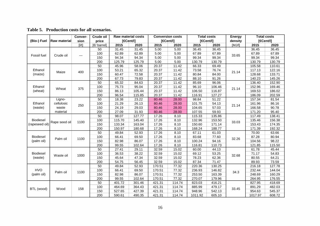
5. Production cost modelling and results

The total production costs for each type of fuel are given by the sum of its raw material price

and its conversion costs. Whereas the former summand has already been projected in Table 3,

the conversion costs have to be projected under consideration of the expected technical status

for the years 2015 and 2020. Production cost analyses for fuels are based on reference scenar-

ios of crude oil prices of €50, €100, €150 and €200 per barrel.

Whereas Table 5 represents the core element of the scenario analysis, the next section de-

scribes how this table is derived and its relationship to the input parameters contained in other

tables and figures. In the subsequent sections 6.2 and 6.3, the results of Table 5 are discussed

and supported by illustrating figures. In the analysis, all monetary amounts are related to the

Euro (€) as the basic currency unless specified differently. In the cases where monetary

amounts are related to a literature reference and is available in US$ only, the corresponding

Euro amount is added in brackets using a foreign exchange rate for € per US$ of 0.69768 per

31 December 2009 for the conversion.

14

5.1. Production costs model

Given the specific conversion technology, the raw material prices are exogenous variables in

the here presented model and independent from the production scale. This is a rough assump-

tion as transport costs are a main driver for biomass prices and the transport costs per unit

increase with scale as transport routes are becoming longer. The rationale behind this assump-

tion is that each company aims to operate at the optimal production scale in light of the ten-

sion between scale benefits on the one hand and increasing cost of capital associated with

transportation costs on the other, which is in line with the results of Nguyen and Prince (1996).

Unlike for raw material costs, cost advantages driven by scale size and learning effects related

to experience are significant endogenous parameters and therefore main determinants in this

calculation model.

Exemplary for 2nd generation ethanol, Table 4 shows the determination of the conversion

costs. For each specific scale size, the required investment volume as well as the operational

costs in million Euros (m €) are estimated based on industrial experience by the authors and

supported by interviews with practical experts. With regard to the initial investment volume,

the average depreciation period is assumed to be 20 years. To account for technical learning

potential on production costs until 2020, learning curve coefficients are estimated and applied

to all process steps as defined in Fig. 1. Depending on the type of fuel, these learning curve

coefficients are specifically estimated and are assumed to show diminishing effects over time.

As exemplary demonstrated in Table 4 for 2nd generation bioethanol, the estimated cost re-

duction potential from learning curve effects are: 40% for the time period 2005-2010, 30% for

time period 2010-2015 and 20% for the time period 2015-2020, which in turn leads to corre-

sponding progress coefficients for the specific time periods of 60%, 70% and 80%, respec-

tively. In an autoregressive time series model, these progress coefficients are sequentially

multiplied with the previous values to derive the operational and total production costs for the

specified points in time. The effect of economies of scale from the size of the production fa-

cility is also reflected in Table 4 and specified for biofuel output scales of 10, 50, 100, 250

and 500 kilo tonnes (kt). Based on the accumulated costs over each step in the production

process, the total conversion costs for each type of biofuel were derived for 2015 and 2020.

The relevant amounts representing the production costs for each type of biofuel are deter-

mined under consideration of the estimated scale size as illustrated in Fig. 2. So for 2nd gen-

eration bioethanol, the relevant total conversion costs are derived by considering the expected

15

Table 4. Modelling of conversion costs for ethanol 2nd generation. Process step 1Learning curve effect 2005-2010: 0.60 Learning curve effect 2010-2015: 0.70 Learning curve effect 2015-2020: 0.80

[kt] [m l] [m €] [m €/ year] [€Cent/l] [m €] [€Cent/l] [m €] [€Cent/l] [m €] [€Cent/l] [m €] [€Cent/l] [m €] [€Cent/l] [m €] [€Cent/l] [m €] [€Cent/l] [m €] [€Cent/l]

10 13 20 1.00 7.90 12.00 94.80 7.20 56.88 5.04 39.82 4.03 31.85 13.00 102.70 8.20 64.78 6.04 47.72 5.03 39.7550 63 70 3.50 5.53 24.00 37.92 14.40 22.75 10.08 15.93 8.06 12.74 27.50 43.45 17.90 28.28 13.58 21.46 11.56 18.27

100 127 100 5.00 3.95 36.00 28.44 21.60 17.06 15.12 11.94 12.10 9.56 41.00 32.39 26.60 21.01 20.12 15.89 17.10 13.51250 316 150 7.50 2.37 48.00 15.17 28.80 9.10 20.16 6.37 16.13 5.10 55.50 17.54 36.30 11.47 27.66 8.74 23.63 7.47500 633 200 10.00 1.58 60.00 9.48 36.00 5.69 25.20 3.98 20.16 3.19 70.00 11.06 46.00 7.27 35.20 5.56 30.16 4.77

Process step 2Learning curve effect 2005-2010: 0.60 Learning curve effect 2010-2015: 0.70 Learning curve effect 2015-2020: 0.80

[kt] [m l] [m €] [m €/ year] [€Cent/l] [m €] [€Cent/l] [m €] [€Cent/l] [m €] [€Cent/l] [m €] [€Cent/l] [m €] [€Cent/l] [m €] [€Cent/l] [m €] [€Cent/l] [m €] [€Cent/l]10 13 30 1.50 11.85 18.00 142.20 10.80 85.32 7.56 59.72 6.05 47.78 19.50 154.05 12.30 97.17 9.06 71.57 7.55 59.6350 63 105 5.25 8.30 36.00 56.88 21.60 34.13 15.12 23.89 12.10 19.11 41.25 65.18 26.85 42.42 20.37 32.18 17.35 27.41

100 127 150 7.50 5.93 54.00 42.66 32.40 25.60 22.68 17.92 18.14 14.33 61.50 48.59 39.90 31.52 30.18 23.84 25.64 20.26250 316 225 11.25 3.56 72.00 22.75 43.20 13.65 30.24 9.56 24.19 7.64 83.25 26.31 54.45 17.21 41.49 13.11 35.44 11.20500 633 300 15.00 2.37 90.00 14.22 54.00 8.53 37.80 5.97 30.24 4.78 105.00 16.59 69.00 10.90 52.80 8.34 45.24 7.15

Process step 3Learning curve effect 2005-2010 0.60

[kt] [m l] [m €] [m €/ year] [€Cent/l] [m €] [€Cent/l] [m €] [€Cent/l] [m €] [€Cent/l] [m €] [€Cent/l] [m €] [€Cent/l] [m €] [€Cent/l] [m €] [€Cent/l] [m €] [€Cent/l]10 13 25 1.25 9.88 15.00 118.50 9.00 71.10 6.30 49.77 5.04 39.82 16.25 128.38 10.25 80.98 7.55 59.65 6.29 49.6950 63 88 4.38 6.91 30.00 47.40 18.00 28.44 12.60 19.91 10.08 15.93 34.38 54.31 22.38 35.35 16.98 26.82 14.46 22.84

100 127 125 6.25 4.94 45.00 35.55 27.00 21.33 18.90 14.93 15.12 11.94 51.25 40.49 33.25 26.27 25.15 19.87 21.37 16.88250 316 188 9.38 2.96 60.00 18.96 36.00 11.38 25.20 7.96 20.16 6.37 69.38 21.92 45.38 14.34 34.58 10.93 29.54 9.33500 633 250 12.50 1.98 75.00 11.85 45.00 7.11 31.50 4.98 25.20 3.98 87.50 13.83 57.50 9.09 44.00 6.95 37.70 5.96

Total process

[kt] [m l] [m €] [m €/ year] [€Cent/l] [m €] [€Cent/l] [m €] [€Cent/l] [m €] [€Cent/l] [m €] [€Cent/l] [m €] [€Cent/l] [m €] [€Cent/l] [m €] [€Cent/l] [m €] [€Cent/l]10 13 75 3.75 29.63 45.00 355.50 27.00 213.30 18.90 149.31 15.12 119.45 48.75 385.13 30.75 242.93 22.65 178.94 18.87 149.0750 63 263 13.13 20.74 90.00 142.20 54.00 85.32 37.80 59.72 30.24 47.78 103.13 162.94 67.13 106.06 50.93 80.46 43.37 68.52

100 127 375 18.75 14.81 135.00 106.65 81.00 63.99 56.70 44.79 45.36 35.83 153.75 121.46 99.75 78.80 75.45 59.61 64.11 50.65250 316 563 28.13 8.89 180.00 56.88 108.00 34.13 75.60 23.89 60.48 19.11 208.13 65.77 136.13 43.02 103.73 32.78 88.61 28.00500 633 750 37.50 5.93 225.00 35.55 135.00 21.33 94.50 14.93 75.60 11.94 262.50 41.48 172.50 27.26 132.00 20.86 113.10 17.87

Total costs = operational expenses plus depreciation2005 2010 2015 2020 2005

Scale Invest-ment

DepreciationOperational costs

Scale Invest-ment

DepreciationOperational costs

2005 2010 2015 2020

2010 2015 2020

Total costs = operational expenses plus depreciation2015 2020 2005 2010

Total costs = operational expenses plus depreciation2005 2010 2015 2020 2005

Scale Invest-ment

DepreciationOperational costs

Scale Invest-ment

DepreciationOperational costs

2005 2010 2015 2020

2010 2015 2020

Total costs = operational expenses plus depreciation2015 2020 2005 2010

16

Table 5. Production costs for all scenarios.

Conver-sion

Crude oil price

[l/t] [€/ barrel] 2015 2020 2015 2020 2015 2020 2015 202050 31.45 31.45 5.00 5.00 36.45 36.45 36.45 36.45

100 62.89 62.89 5.00 5.00 67.89 67.89 67.89 67.89150 94.34 94.34 5.00 5.00 99.34 99.34 99.34 99.34200 125.79 125.79 5.00 5.00 130.79 130.79 130.79 130.7950 45.96 58.06 20.37 11.42 66.33 69.49 105.58 110.61

100 53.21 65.32 20.37 11.42 73.58 76.74 117.13 122.16150 60.47 72.58 20.37 11.42 80.84 84.00 128.68 133.71200 67.73 79.83 20.37 11.42 88.10 91.26 140.23 145.2650 65.32 84.63 20.37 11.42 85.69 96.06 136.40 152.90

100 75.73 95.04 20.37 11.42 96.10 106.46 152.96 169.46150 86.13 105.44 20.37 11.42 106.50 116.87 169.53 186.02200 96.54 115.85 20.37 11.42 116.91 127.27 186.09 202.5950 18.38 23.22 80.46 28.00 98.84 51.22 157.34 81.54

100 21.29 26.13 80.46 28.00 101.75 54.13 161.96 86.16150 24.19 29.03 80.46 28.00 104.65 57.03 166.58 90.78200 27.09 31.93 80.46 28.00 107.55 59.93 171.20 95.4050 98.07 127.77 17.26 8.10 115.33 135.86 117.49 138.41

100 115.70 145.40 17.26 8.10 132.96 153.50 135.46 156.38150 133.34 163.04 17.26 8.10 150.60 171.14 153.43 174.35200 150.97 180.68 17.26 8.10 168.24 188.77 171.39 192.3250 49.84 52.93 17.26 8.10 67.11 61.03 70.00 63.66

100 66.41 69.50 17.26 8.10 83.68 77.60 87.28 80.94150 82.98 86.07 17.26 8.10 100.24 94.16 104.56 98.22200 99.55 102.64 17.26 8.10 116.81 110.73 121.85 115.5050 27.41 29.11 32.59 15.02 60.00 44.13 61.78 45.44

100 36.53 38.22 32.59 15.02 69.12 53.25 71.17 54.83150 45.64 47.34 32.59 15.02 78.23 62.36 80.55 64.21200 54.75 56.45 32.59 15.02 87.34 71.47 89.93 73.5950 49.84 52.93 170.51 77.32 220.36 130.25 216.18 127.78

100 66.41 69.50 170.51 77.32 236.93 146.82 232.44 144.04150 82.98 86.07 170.51 77.32 253.50 163.39 248.69 160.29200 99.55 102.64 170.51 77.32 270.07 179.96 264.95 176.5550 401.72 301.46 421.31 114.74 823.03 416.21 827.95 418.69

100 464.69 364.43 421.31 114.74 885.99 479.17 891.29 482.03150 527.65 427.39 421.31 114.74 948.96 542.13 954.63 545.37200 590.61 490.35 421.31 114.74 1011.92 605.10 1017.97 608.72

(Bio-) Fuel Raw materialEnergy density

[MJ/l]

Total costs[€Cent/l]

Ethanol (waste)

Ligno-cellulosic

waste material

Fossil fuel Crude oil

Total costs[€Cent/l]

Conversion costs [€Cent/l]

Raw material costs [€Cent/l]

1000

--- 33.65

21.14

21.14

1100

158

400

375

250

1100

1100Biodiesel (palm oil)

Palm oil

Biodiesel (waste)

Waste oil

BTL (wood) Wood

Ethanol (maize)

Maize

Ethanol (wheat)

Wheat

HVO (palm oil)

Palm oil

Biodiesel (rapeseed oil)

Rape seed oil

33.45

21.14

33.03

32.26

32.68

34.3

17

scale sizes of 50kt for 2015 and 250kt for 2020. This results in conversion costs of €Cent 80/l

and €Cent 28/l for the respective reference years.

These amounts are then used for all further calculations and Table 5 also shows these assumed

conversion costs in Euro cent per litre (€Cent/l) of fuel output for the forecasted years 2015

and 2020. These amounts are added to the corresponding raw material costs to determine the

total production costs. Furthermore, to ensure the comparability of the total costs for each

type of biofuel, the energy density factor in Millijoule per litre (MJ/l) has to be taken into

consideration. By this measure, the total production costs for each type of biofuel are normal-

ised on the average energy density of fossil fuel, to account for variations in the energy den-

sity of the biofuels. Particularly the total costs for ethanol fuels have to be revised upwards,

due to the low energy density factor of 21.14 MJ/l, which is about 37% lower than the energy

density factor of 33.65 MJ/l for fossil fuel.

In consequence, this led to some significant adjustments in the production costs based on the

specific energy density of biofuels. With these data, the production costs for the reference

scenarios of all relevant biofuels in 2010, 2015 and 2020 are calculated. This model enables

the calculation for different production scales in place and planned or hypothetical scales (e.g.

simulation of not yet realised production scales).

5.2. Estimations of biofuel production costs in 2015

As presented in Table 5 and illustrated in Fig. 4 below, for 2015 the results obtained from

modelling the production costs for various biofuels indicate that there is no biofuel that can be

produced at competitive costs compared to fossil fuel (€Cent 68/l) under the assumption of a

crude oil price of €100/barrel. However, with total production costs of €Cent 71/l and €Cent

87/l for biodiesel from waste oil and from palm oil, the gap towards fossil fuel is relatively

small for these two types of biofuel.

Similarly, in the case of a crude oil price of €200/barrel, the production costs for most types of

biofuels exceed those for fossil fuel (€Cent 131/l). Even under this extremely negative crude

oil price scenario, the only biofuels that are most likely to be competitive are biodiesel from

waste oil (€Cent 90/l) and biodiesel from palm oil (€Cent 122/l). Compared to these types of

biodiesels, the production costs for bioethanol from lignocellulosic waste material are higher

in all crude oil price scenarios, e.g. €Cent 171/l given a crude oil price of €200/barrel. Fur-

thermore, unlike for other biofuels, the simulation of different crude oil price scenarios in Fig.

18

3 indicates that production costs for bioethanol from lignocellulosic waste is largely inde-

pendent of the crude oil price levels. Besides this, the simulation in Fig. 3 reveals that produc-

tion costs of HVO and BTL are significantly above all fuels and for economic reasons they do

not appear as a reasonable alternative. As it becomes obvious by the comparison in Table 5,

the uncompetitive total costs for HVO and BTL are mainly due to the excessive conversion

costs in 2015 of €Cent 421/l and €Cent 171/l, respectively. This reflects that the scale and

learning effects have not yet generated their full impact on the conversion costs by 2015.

Fig. 3. Production costs in the year 2015.

0

200

400

600

800

1000

1200

Fossil

fuel

Ethan

ol (m

aize)

Ethan

ol (w

heat

)

Ethan

ol (w

aste

)

Biodies

el (ra

pese

ed o

il)

Biodies

el (p

alm o

il)

Biodies

el (w

aste

)

HVO (p

alm o

il)

BTL (w

ood)

Pro

du

ctio

n c

ost

s [€

Ce

nt/

l]

50 100 150 200

Scenarios for crude oil price in 2015 (US-$ per barrel):

5.3. Estimations of biofuel production costs in 2020

Even when taking into account the scale and learning effects on the conversion costs for the

time period until 2020, no biofuel can be produced competitively to fossil fuel at crude oil

prices €50 per barrel (Table 5 and Fig. 4). Given a crude oil price of €100 per barrel, accord-

ing the here presented model, the most promising biofuel is biodiesel from waste oil (€Cent

55/l) with even lower costs than fossil fuel (€Cent 68/l), followed by biodiesel from palm oil

(€Cent 81/l) and bioethanol from lignocellulosic waste (€Cent 86/l). Assuming a market price

for crude oil of €150/barrel in 2020 (Fig. 5), ethanol from lignocellulosic waste (€Cent 91/l)

and biodiesel from both, waste oil (€Cent 64/l) and palm oil (€Cent 98/l) can be produced at

19

Fig. 4. Production costs in the year 2020.

0

100

200

300

400

500

600

700

Fossil

fuel

Ethan

ol (m

aize)

Ethan

ol (w

heat

)

Ethan

ol (w

aste

)

Biodies

el (ra

pese

ed o

il)

Biodies

el (p

alm o

il)

Biodies

el (w

aste

)

HVO (p

alm o

il)

BTL (w

ood)

Pro

du

ctio

n c

ost

s [€

Cen

t/l]

50 100 150 200

Scenarios for crude oil price in 2020 (US-$ per barrel):

Fig. 5. Production costs at 150 Euro/barrel crude oil in 2015 and 2020.

0

200

400

600

800

1000

1200

Fossil

fuel

Ethan

ol (m

aize)

Ethan

ol (w

heat

)

Ethan

ol (w

aste

)

Biodies

el (ra

pese

ed o

il)

Biodies

el (p

alm o

il)

Biodies

el (w

aste

)

HVO (p

alm o

il)

BTL (w

ood)

Pro

du

ctio

n c

ost

s [€

Ce

nt/

l]

2015 2020

20

competitive costs, below those for fossil fuel (€Cent 99/l). Whereas the first two types of bio-

fuels can be produced even cheaper than fossil fuel, the production costs for the latter are al-

most the same as those for fossil fuel from crude oil. Similarly, in the scenario of a market

price for crude oil of €200/barrel there are three types of biofuels that can be produced at

lower costs compared to fossil fuel (€Cent 131/l): biodiesel from waste oil (€Cent 74/l), etha-

nol from lignocellulosic waste (€Cent 95/l) as well as biodiesel from palm oil (€Cent 116/l).

6. Discussion

6.1. Implications from the 2015 and 2020 scenarios

As the results in Table 5 demonstrate, the total production costs for each type of fuel are pri-

marily driven by the market price of the underlying raw materials. In contrast, the conversion

costs only play a subordinate role, particularly the more the projection goes further into the

future and towards larger production scales. With regard to the drivers of the conversion costs,

the results indicate that the total conversion costs can be primarily reduced by scale effects,

given the assumptions specified for the learning curve coefficients and production scale size

level (the initial investment as well as operational costs). Exemplary for all types of biofuels

covered in this study, Table 4 shows that the total conversion costs can be reduced to roughly

one tenth solely through scale economies associated with an upscaling of the production plant

size from 10kt to 500kt, e.g. from €Cent 149/l to €Cent 18/l in the 2020 scenario. In contrast,

between 2005 and 2020 the expected reduction of the conversion costs attributable to learning

effects is approximately half, resulting from the combination of the learning curve coefficients

during this time period.

In total, despite positive learning and scale effects, 1st generation bioethanol as well as 1st

generation biodiesel show increasing total production costs between 2015 and 2020, which is

due to the high level of raw material prices. This increase in total production costs pertains to

all 1st generation biofuels except biodiesel from palm oil, where the advancements in produc-

tion processes overcompensate rising feedstock prices.

Similarly, HVO, and particularly BTL, are uncompetitive because of relatively high raw ma-

terial costs combined with high conversion costs. Although HVO, and especially BTL, are

associated with considerable lower conversion costs due to learning effects in 2020 compared

to 2015, the related cost saving potentials are not sufficient to compensate the high raw mate-

rial costs. Consequently, HVO and BTL are not expected to be produced at competitive costs

21

even though both have a higher energy density compared to other biofuels, in particular to

bioethanol.

Taking into account positive effects from learning and scale size in all crude oil price scenar-

ios, 2nd generation biofuels show the highest cost saving potentials until 2020. Biodiesel from

waste oil and bioethanol produced on a large scale from lignocellulose containing raw materi-

als are the most promising with regard to total production costs.

The results obtained from modelling the total production costs of (bio-) fuels demonstrate that

2nd generation biodiesel from waste oil is the most cost competitive fuel followed by bio-

ethanol from lignocellulosic waste material. This is in line with the research results from de

Wit et al. (2010), who explain this order between those two types of biofuels by lower feed-

stock, capital and operational costs. Unlike bioethanol, the production of biodiesel is associ-

ated with lower feedstock costs for oil crops compared to sugar and starch crops. Furthermore,

biodiesel requires relatively lower capital and operational expenses for transesterification of

oil to biodiesel compared to hydrolysis and fermentation of sugar and starch crops to bioetha-

nol. This initial advantage of biodiesel over bioethanol, however, may impede the exploitation

of positive effects associated with learning and a larger scope and, in consequence, may pre-

vent the use of related cost saving potentials for bioethanol.

6.2. Influence of economic policies on biofuels

Owing to the continuously increasing demand in crude oil aligned with lagged increase in

supply and thus rising crude oil prices, the attractiveness of alternative fuels is growing.

Compared to conventional fuels, competitive production costs are essential to gain market

share as the current tax advantages are only temporary.

Since 2002, the Brazilian government has launched several national programmes to enhance

its technical, economic, and environmental competitiveness of biodiesel production in relation

to fossil fuel and has achieved considerable progress, especially due to its richness in required

raw materials (Ramos and Wilhelm, 2005; Nass et al., 2007). For bioethanol from Brazil,

however, an import tariff of US$Cent 54 (€Cent 0,38) per gallon (de Gorter and Just, 2009;

Lamers et al., 2011) that had been established due to economic and environmental reasons,

impeded market access in the United States until 2012. With very competitive production

costs in the range of approximately US$Cent 34/l (€Cent 0,24/l) in 2009 and an estimated

range between US$Cent 20/l (€Cent 14/l) and US$Cent 26/l (€Cent 18/l) (van den Wall Bake

22

et al., 2009), import tariffs are a decisive factor for the market acceptance of Brazilian bio-

diesel.

In the European Union, biofuel policies on national and international level enhanced the gen-

eral demand for biofuels and simultaneously stimulated the production (Lamers et al., 2011).

Primarily for 1st generation biofuels, the European Union itself is not able to domestically

produce sufficient biofuel feedstock to fulfil these policies, so it is forced to import biofuel

crops and run a higher agricultural trade deficit. Simultaneously, this leads to additionally

increasing biofuel crop production in other countries with a comparative advantage, especially

in South and Central American countries like Brazil (Banse et al., 2011).

The results of this study indicate that the total production costs for all types of fuels are

mainly driven by the market price of the underlying raw materials and that a considerable

reduction of the conversion costs can only be achieved by an extensive increase in the produc-

tion scale. However, ignoring the market price for raw materials, the realisation of a corre-

sponding increase in the production scale requires a volume of biomass feedstock that can

hardly be generated, particularly when taking into account the demanded quantity and the

European land size.

6.3. Methodological limitations and recommendations for further research

The most important limitation of this analysis is associated with the future development of the

raw material prices. The study is based on the assumption that 1) the development of biofuel

feedstock prices and market prices for crude oil can be extrapolated to future periods and that

2) the raw material prices are exogenous variables and not endogenously affected by the pro-

duction of biofuels. As such, the study takes the perspective of a biofuel producer acting as a

price taker, without influence on the market price of the raw materials. However, the market

prices of related feedstock depend on numerous factors, some of which are interdependent,

and therefore hard to anticipate. For 1st generation biofuels, various studies (Mitchell, 2008;

Lipsky, 2008; Headey, 2008) investigating the future development and relevant impact factors

have shown that biofuels are a main driver of increasing feedstock prices. The prices for lig-

nocellulose biomass underlying 2nd generation biofuels have not been as thoroughly investi-

gated as those for 1st generation biofuels, even though raw material costs are certainly the

main driver for total production costs. In this regard, Gnansounou and Dauriat (2010) con-

clude that in the medium to long term, besides biofuels, lignocellulosic raw materials are in-

creasingly being used also for chemicals and materials. As a result, there is rising demand and

23

competition for these resources pertaining various technical applications including both en-

ergy and non-energy uses.

Another limitation in this analysis is that it does not distinguish between diesel and petrol

substitute markets. This approach is in line with de Wit (2010), who reference to the current

European policy, which does not differentiate the biofuel targets, and note that a separation

may lead to a suboptimal allocation of technological efforts and feedstock between the two

fuel types.

7. Conclusions

As the price is the decisive factor for a fuel’s market acceptance, competitive production costs

are essential in order to establish biofuels as an alternative source to fossil sources. This re-

search paper focuses on future production cost developments and follows three objectives: 1)

projection of future biomass prices partly based on the change of crude oil prices, 2) simula-

tion of not yet realised scale and learning effects in the production of biofuels; and 3) com-

parison of the competitiveness of different biofuels and fossil fuels. This study demonstrated

that modelling biofuel production costs based on three standardised production process steps

enables a better understanding of cost competitiveness. Furthermore, unlike many other stud-

ies in the field of biofuels, this paper provides a macro-economic driven bottom-up approach

in order to compare different types of fuels and gives insights to future price developments

that are useful for producers as well as consumers. In this context, as one of very few studies,

the calculation model presented takes into account the effects from technological learning and

production scale and enables a justified discussion about the future potential of certain types

of fuels among academics as well as practitioners. As the most important model parameter,

besides the crude oil price, the price development of the underlying biomass raw materials is

endogenously projected by the price index for agricultural products, growth in world popula-

tion, growth in wealth per capita income, and change in energy consumption per capita. The

results show that the total production costs for each type of fuel is primarily driven by the

market price of the underlying raw materials. In contrast, the conversion costs are only of mi-

nor importance, particularly the more the projection goes further into the future and towards

larger production scales. With regard to the drivers of the conversion costs, the results indi-

cate that the total conversion costs can be primarily reduced by scale effects and that the ef-

fect from technological learning has only a limited impact on the conversion costs and thus on

the total production costs.

24

In general, 1st generation biofuels are produced from expensive feedstock with established

and optimised technologies, while the 2nd generation are associated with relatively lower raw

material costs and increasing efficiencies due to advanced conversion processes. Over the

short and medium term, 2nd generation biodiesel from waste oil and from palm oil are the

most promising with regard to production costs. Even given a crude oil price of €200/barrel in

2015, the only biofuels that are most likely to be competitive are biodiesel from waste oil and

biodiesel from palm oil.

Particularly for 2nd generation biofuels, the competiveness will additionally increase mid- to

long-term due to economies of scale and learning curve effects. In this time horizon, bioetha-

nol from lignocellulose biomass as well as biodiesel from waste oil and palm oil show high

cost saving potentials which enable highest yields. So mid- to long-term, at all oil price sce-

narios, 2nd generation biofuels are most likely to be produced competitively. Except for bio-

diesel from palm oil, the production costs of 1st generation biofuels exceed those for fossil

fuel and they are thus associated with a poor financial performance. In particular, this applies

when additionally taking into account even increasing feedstock costs. As cost saving poten-

tials from production scale have already been exploited to a large extend, any further competi-

tive improvements of 1st generation biofuels can only be realised by experience-driven learn-

ing effects.

However, for all types of biofuels remains a serious doubt whether a sufficient amount of

feedstock can be generated to satisfy the growing demand and to achieve the shift from fossil

fuel to biofuels.

8. References

Ajanovic, A., 2011. Biofuels versus food production: Does biofuels production increase food

prices? Energy 36, 2070-2076.

Antoni, D., Zverlov, V., Schwarz, W., 2007. Biofuels from microbes. Applied Microbiology

and Biotechnology 77, 23-35.

Araujo, V.K., Hamacher, S., Scavarda, L.F., 2010. Economic assessment of biodiesel produc-

tion from waste frying oils. Bioresource Technology 101, 4415-4422.

Bagheri, A., 2011. Opec's Role in the Diversified Future Energy Market. Iranian Journal of

Economic Research 16, 1-18.

25

Balat, M., 2011. Production of bioethanol from lignocellulosic materials via the biochemical

pathway: A review. Energy Conversion and Management 52, 858-875.

Banse, M., van Meijl, H., Tabeau, A., Woltjer, G., Hellmann, F., Verburg, P.H., 2011. Impact

of EU biofuel policies on world agricultural production and land use. Biomass & Bio-

energy 35, 2385-2390.

Berghout, N.A., 2008. Technological learning in the german biodiesel industry: an experience

curve approach to quantify reductions in production costs, energy use and greenhouse gas

emissions. Utrecht University, Netherlands. Retrieved on 8 June 2013,

from.http://www.task39.org/LinkClick.aspx?fileticket=vbqVpmG%2Fh8Y%3D&tabid=44

26&language=en-US

Birol, F., 2010. World Energy Outlook 2010. International Energy Agency, Paris, France.

Blok, K., 2006. Introduction to energy analysis. Techne Press, Amsterdam, Netherlands.

Bomb, C., McCornic, K., Deurwaarder, E., Kaberger, T., 2007. Biofuels for transport in

Europe: Lessons from Germany and the UK. Energy Policy 35, 2256-2267.

Bridgewater, A.V., Double, M., 1994. Production costs of liquid fuels from biomass. Interna-

tional Journal of Energy Research 18, 79-94.

Chen, S.-T., Kuo, H.-I., Chen, C.-C., 2010. Modeling the relationship between the oil price

and global food prices. Applied Energy 87, 2517-2525.

Cherubini, F., 2010. The biorefinery concept: Using biomass instead of oil for producing en-

ergy and chemicals. Energy Conversion and Management 51, 1412-1421.

Clark, J.H., 2007. Green chemistry for the second generation biorefinery-sustainable chemical

manufacturing based on biomass. Journal of Chemical Technology & Biotechnology 82,

603-609.

Dautzenberg, K., Hantl, J., 2008. Biofuel chain development in Germany: Organisation, op-

portunities, and challenges. Energy Policy 36, 465-489.

de Gorter, H., Just, D.R., 2009. The welfare economics of a biofuel tax credit and the interac-

tion effects with price contingent farm subsidies. American Journal of Agricultural Eco-

nomics 91, 477-488.

26

de Wit, M., Junginger, M., Lensink, S., Londo, M., Faaij, A., 2010. Competition between bio-

fuels: Modeling technological learning and cost reductions over time. Biomass & Bio-

energy 34, 203-217.

Dixon, P.B., Osborne, S., Rimmer, M.T., 2007. The Economy-wide effects in the United

States of replacing crude petroleum with biomass, Energy & Environment 18, 710-72.

EU-Commission, 2003. Directive 2003/30/EC of the European Parliament and of the Council

of 8 May 2003 on the promotion of the use of Biofuels or other renewable Fuels for Trans-

port. Official Journal of the European Union 5.

Faaij, A.P.C., Meuleman, B., Van Ree, R., 1998. Long term perspectives of biomass inte-

grated/combined cycle (BIG/CC) technology: costs and electrical efficiency. Novem,

Utrecht, Netherlands.

Fargione, J., Hill, J., Tilman, D., Polasky, S., Hawthorne, P., 2008. Land Clearing and the

Biofuel Carbon Debt. Science 319, 1235-1238.

Fernando, S., Adhikari, S., Chandrapal, C., Murali, N., 2006. Biorefineries: Current Status

Challenges and future Direction. Energy & Fuels 20, 1727-1737.

Festel, G., 2007. Biofuels – Which is the Most Economic One? Chimia 61, 744-749.

Festel, G., 2008. Biofuels - Economic Aspects. Chemical Engineering & Technology 31, 715-

720.

Francesco, C., 2010. The biorefinery concept: Using biomass instead of oil for producing en-

ergy and chemicals, Energy Conversion and Management 51, 1412-1421.

Giampietro, M., Ulgiati, S., 2005. Integrated Assessment of Large-Scale Biofuel Production.

Critical Reviews in Plant Sciences 24, 365-384.

Gnansounou, E., Dauriat, A., Villegas, J., Panichelli, L., 2009. Life cycle assessment of bio-

fuels: Energy and greenhouse gas balances. Bioresource Technology 100, 4919-4930.

Gnansounou, E., Dauriat, A., 2010. Techno-economic analysis of lignocellulosic ethanol: A

review. Bioresource Technology 101, 4980-4991.

Gustavsson, L., 1997. Energy efficiency and competitiveness of biomass-based energy sys-

tems, Energy 22, 959-967.

Haldi, J., Whitcomb, D., 1967. Economies of scale in industrial plants. The Journal of Politi-

cal Economy 75, 373–385.

27

Hamelinck, C.N., Van Hooijdonk, G., Faaij, A.P.C., 2005. Ethanol from lignocellulosic bio-

mass: techno-economic performance in short-, middle- and long-term. Biomass & Bio-

energy 28, 384–410.

Harvey, A.C., 1993. Time Series Models. 2nd ed. MIT Press, Cambridge, USA.

Headey, D., Fan, S., 2008. Anatomy of a crisis: The causes and consequences of surging food

prices. Agricultural Economics 39, 375-391.

Hermann, B.G., Patel, M., 2007. Today’s and tomorrow’s bio-based bulk chemicals from

white biotechnology - A techno-economic analysis. Applied Biochemistry and Biotechnol-

ogy 136, 361-388.

Hettinga, W.G., Junginger, H.M., Dekker, S.C., Hoogwijk, M., McAloon, A.J., Hicks, K.B.,

2009. Understanding the reductions in US corn ethanol production costs: An experience

curve approach. Energy Policy 37, 190-203.

Hodge, C., 2008. What is the outlook for renewable diesel? Hydrocarbon Processing 87, 85 -

92.

Hollander, S., 1965. The Sources of Increased Efficiency: A Study of DuPont Rayon Plants.

MIT Press, Cambridge, USA.

IEA, 2007. World energy outlook 2007. OECD/IEA, Paris, France. Retrieved on 4 June 2013,

from http://www.worldenergyoutlook.org/media/weowebsite/2008-1994/weo_2007.pdf

Junginger, M., de Visser, E., Hjort-Gregersen, K., Koornneef, J., Raven, R., Faaij, A., 2006.

Technological learning in bioenergy systems. Energy Policy 34, 4024–4041.

Kim, S., Dale, B.E., 2004. Global potential bioethanol production from wasted crops and crop

residues. Biomass & Bioenergy 26, 361-375.

Kim, J., Realff, M.J., Lee, J.H., Whittaker, C., Furtner, L., 2011. Design of biomass process-

ing network for biofuel production using an MILP model. Biomass & Bioenergy 35, 853-

871

Klein-Marcuschamer, D., Oleskowicz-Popiel, P., Simmons, B.A., Blanch, H.W., 2012. The

Challenge of Enzyme Cost in the Production of Lignocellulosic Biofuels, Biotechnology

and Bioengineering 109, 1083-1087.

28

Lamers, P., Hamelinck, C., Junginger, M., Faaij, A., 2011. International Bioenergy Trade: A

Review of Past Developments in the Liquid Biofuel Market. Renewable and Sustainable

Energy Reviews 15, 2655-2676.

Leistritz, F.L., Hodur, N.M., 2008. Biofuels: a major rural economic development opportunity.

Biofuels Bioproducts & Biorefining 2, 501-504.

Lieberman, M.B., 1984. The learning curve and pricing in the chemical processing industries.

The RAND Journal of Economics 15, 213-228.

Lipsky, J., 2008. Commodity Prices and Global Inflation. Remarks by the First Deputy Man-

aging Director of the IMF at the Council on Foreign Relations, 8 May 2008, New York,

USA. Retrieved on 3 June 2013, from http://www.imf.org/external/np/speeches/

2008/050808.htm.

Martinsen, D., Funk, C., Linssen, J., 2010. Biomass for transportation fuels - A cost-effective

option for the German energy supply? Energy Policy 38, 128-140.

Mikkonen, S., 2008. Second-generation renewable diesel offers advantages. Hydrocarbon

Processing 87, 63 - 66.

Mitchell, D., 2008. A Note on Rising Food Prices. Policy Research Working Paper #4682.

World Bank, Development Prospects Group, Washington, DC.

Mizsey, P., Racz, L., 2010. Cleaner production alternatives: Biomass utilisation options,

Journal of Cleaner Production 18, 767-770.

Naik, S.N., Goud, V.V., Rout, P.K., Dalai, A.K., 2010. Production of first and second genera-

tion biofuels: A comprehensive review. Renewable and Sustainable Energy Reviews 14,

578–597.

Nass, L.L., Pereira, P.A.A., Ellis, D., 2007. Biofuels in Brazil: An overview. Crop Science 47,

2228-2237.

National Renewable Energy Laboratory (NREL), Process Design and Economics for Bio-

chemical Conversion of Lignocellulosic Biomass to Ethanol - Dilute-Acid Pretreatment

and Enzymatic Hydrolysis of Corn Stover, May 2011, Golden, USA. Retrieved on 6 June

2013, from http://www.nrel.gov/docs/fy11osti/47764.pdf.

29

Nguyen, M.H., Prince, R.G.H., 1996. A simple rule for bioenergy conversion plant size opti-

misation: Bioethanol from sugar cane and sweet sorghum. Biomass & Bioenergy 10, 361-

365.

Parry, I., Williams, R.C., Goulder, L.H., 1999. When can carbon abatement policies increase

welfare? The fundamental role of distorted factor markets. Journal of Environmental Eco-

nomics and Management 37, 52-84.

Preston, L., Keachie, E.C., 1964. Cost Functions and Progress Functions: An Integration.

American Economic Review 54, 100-107.

Ramos, L.P., Wilhelm, H.M., 2005. Current Status of Biodiesel Development in Brazil. Ap-

plied Biochemistry and Biotechnology 121-124, 807-820.

Stephen, J.D., Mabee, W.E., Saddler, J.N., 2010. Biomass logistics as a determinant of sec-

ond-generation biofuel facility scale, location and technology selection. Biofuels Biopro-

ducts & Biorefining 4, 503-518.

Stobaugh, R.B., Townsend, P.L., 1975. Price Forecasting and Strategic Planning: The Case of

Petrochemicals. Journal of Marketing Research 12, 19-29.

Sultan, R.G.M., 1975. Pricing in the Electrical Oligopoly, Vol. 2. Division of Research,

Graduate School of Business Administration, Harvard University, Cambridge, USA.

Swinnen, J., Tollens, E., 1991. Bulk Chemicals from biomass in the EC: Feasibility and po-

tential outlets. Bioresource Technology 36, 277-291.

Tufvesson, P., Lima-Ramos, J., Nordblad, M., Woodley, J.M., 2011. Guidelines and Cost

Analysis for Catalyst Production in Biocatalytic Processes, Organic Process Research &

Development 15, 266–274

Tyner, W.E., Taheripour, F., 2008. Policy Options for Integrated Energy and Agricultural

Markets. Review of Agricultural Economics 30, 387–396.

U.S. EIA, 2011. Annual Energy Outlook 2011: With projections to 2035. U.S. Energy Infor-

mation Administration, Washington, DC, USA.

Uyterlinde, M.A., Junginger, H.M., De Vries, H.J., Faaij, A.P.C., Turkenburg, W.C., 2007.

Implications of technological learning on the prospects for renewable energy technologies

in Europe. Energy Policy 35, 4072–4087.

30

van den Wall Bake, J.D., Junginger, H.M, Faaij, A.P.C., Poot, T., Walter, A., 2009. Explain-

ing the experience curve: cost reductions of Brazilian ethanol from sugarcane. Biomass &

Bioenergy 33, 644–658.

van Kasteren, J., Nisworo, A., 2007. A process model to estimate the cost of industrial scale

biodiesel production from waste cooking oil by supercritical transesterification. Resources,

Conservation and Recycling 50, 442-458.

West, A.H., Posarac, D., Ellis, N., 2008. Assessment of four biodiesel production processes

using HYSYS.Plant. Bioresource Technology 99, 6587-6601.

Zhang, Y., Dubé, M., McLean, D., Kates, M., 2003. Biodiesel production from waste cooking

oil: 2. Economic assessment and sensitivity analysis. Bioresource Technology 90, 229-240.