Modelling price formation and dynamics in the Ethiopian maize...

Modelling price formation and dynamics in the

Ethiopian maize market

Mesay Yami, Ferdi Meyer and Rashid Hassan

Invited poster presented at the 5th

International Conference of the African Association

of Agricultural Economists, September 23-26, 2016, Addis Ababa, Ethiopia

Copyright 2016 by [authors]. All rights reserved. Readers may make verbatim copies of

this document for non-commercial purposes by any means, provided that this copyright

notice appears on all such copies.

1

Modelling price formation and dynamics in the Ethiopian maize market

Mesay Yami1*

, Ferdi Meyer2 and Rashid Hassan

3

1Department of Agricultural Economics, Extension & Rural Development, University of Pretoria, South Africa;

2Bureau for Food and Agricultural Policy (BFAP), University of Pretoria, South Africa

3Centre for Environmental Economics and Policy Analysis (CEEPA), University of Pretoria, South Africa;

* Corresponding author Email: [email protected]

2

Abstract

In response to the sharp rise in domestic grain prices of 2008, the Ethiopian government

introduced a wide range of policy instruments to tame the soaring domestic food prices. It is

generally argued that before embarking on any intervention in domestic grain market, better

understanding of price formation and possible scenarios of the dynamic grain market

environment is crucial for policymakers to make informed decisions. This study aimed at

examining the price formation and dynamics in the Ethiopian maize market. Furthermore,

this article empirically investigate spatial maize market linkages and test maize price

leadership role in order to understand as to whether or not there is a central maize market that

dictate and lead price information flow over regional maize markets in Ethiopia.

Keywords: Grain market; price shocks; maize; market integration; price formation

3

1. INTRODUCTION

Recently, the Ethiopian grain markets have been characterised by price spikes. The year on

year change in food price inflation reached all-time high level of 60% in 2008 (FAO, 2015).

Compared to other major crops, maize commodity prices have historically been more

volatile. For instance, maize prices collapsed considerably whenever there are bumper

harvests as was the case in 1995/96, 1996/97, 1999/00, and 2001/02 (RATES, 2003). Maize

prices collapsed by almost 80% and reached the lowest in early 2002. Bumper harvests led to

the significant price drop and created market glut in higher producing areas. Accordingly, the

low market price created disincentive effects for farmers to use improved production

technologies such as commercial fertilizer and improved seed. Compared to 2002, maize

production dropped by 14% and 3% during 2003 and 2004 (FAO, 2015). The lesson learned

by government as well as international and national research organizations with regards to the

unprecedented low maize price episode of 2002 was that crop productivity improvement

alone does not translate into welfare gains of producers. Therefore, agricultural policies that

target farmers’ livelihood improvement through technology adoption and crop productivity

should go hand in hand with market development.

Since 2007, maize prices have shown an upward trend in domestic grain market. The

domestic prices of maize reached close to US$ 350/ton by mid-2009. The recent persistence

of high maize prices in the presence of remarkable growth in domestic maize production and

supply remains a puzzle. Maize production has almost doubled (88%) in Ethiopia since 2004

(USDA, 2015). Despite the price volatility, maize is still continues to be a strategic crop to

Ethiopia’s food security interest.

With the recent turmoil in international food market, “getting market prices right” has

become an important topic for most governments. This is also the case for the Ethiopian

government. In response to the sharp rise in domestic grain prices of 2008, the Ethiopian

government introduced a wide range of policy instruments to tame the soaring domestic food

prices. After the adoption of market liberalisation, the government for the first time has

become heavily involved in commercial wheat imports. As means of domestic supply

stabilisation, the Ethiopian government has also imposed an indefinite export ban on major

cereal crops including maize, sorghum, teff and wheat. It is generally argued that before

embarking on any intervention in domestic grain market, better understanding of the price

formation and possible scenarios of the dynamic grain market environment is crucial for

policy makers to make informed decisions for the betterment of producers, investors, traders

and consumers welfare. The dynamic market environment in which producers and consumers

operate necessitate better understanding of price discovery and dynamics of the product they

produce. It is against this backdrop that commodity modelling can provide valuable

information to assist role players in decision-making.

Several studies have attempted to analyse inter-regional spatial grain market integration in

Ethiopia (Negassa et al. 2004; Getnet et al. 2005; Jaleta and Gebremedhin, 2009; Ulimwengu

et al. 2009; Kelbore, 2013; Tamru, 2013). These studies used different approaches ranging

4

from the primitive correlation analysis to dynamic time series model – Ravallion (1979) and

Error Correction Model (ECM). Newly introduced approaches - Parity Bounds Model (PBM)

and Threshold Autoregressive model (TAR) have also employed to analyse grain market

integration and efficiency in Ethiopia. However, all these studies have emphasised on

analysing the co-movement of prices and efficiency of grain markets in Ethiopia. While

knowing whether inter-regional grain markets are integrated or not provides evidence of price

signals transmission across spatial grain markets, it does not tell us much about price

determination and supply and demand induced grain price instability, which is more useful to

policy makers. No attempt has so far been made to explore the fundamentals of supply and

demand dynamics and drivers of equilibrium price in grain market in Ethiopia. This study is

therefore an attempt to understand price formation and discovery in the Ethiopian maize

market. This article also intends to empirically investigate spatial maize market linkages and

test maize price leadership in order to understand as to whether or not there is a central maize

market that dictate and lead price information flow over regional maize markets in Ethiopia.

Understanding the existence of a central market will make it easier for policymakers to

monitor and intervene price distortion in grain market. Thus, further reducing the costs of

price stabilisation policy.

The rest of the paper is organised as follows. Section two discusses maize price discovery in

Ethiopia. Section three describes the approaches and data sources of the study. Section four

presents the findings obtained from partial equilibrium model, market integration, and price

leadership analysis. Section five concludes.

2. MAIZE PRICE DISCOVERY

In order to understand price formation and likely sources of price instability in the Ethiopian

maize market, it is essential to identify the trade regime where the Ethiopian maize market

operates. The trends of maize Self-Sufficiency Ratio (SSR) of Ethiopia indicates that the

country has been largely self-sufficient in maize production (Figure 1). The SSR for maize

has fluctuated between 94% and 102% implying that Ethiopia is trading in autarky trade

regime. In autarky trade regime, domestic maize price is expected to be unrelated to

international market price shocks. Rather, the dynamics of domestic supply and demand

factors apart from government policies are responsible for maize price formation and

instability.

5

Figure 1. Average trends of maize SSR, (1980-2015)

Source: Author’s calculation using USDA data (2015)

3. METHOD OF ANALYSIS

3.1 Data source

The study relied on data obtained from different sources including FAO, USDA, Central

Statistical Agency of Ethiopia (CSA), Ethiopian Grain Trade Enterprise (EGTE), and

National Meteorological Agency of Ethiopia (NMA). Time series data on producer prices of

maize commodity are obtained from FAO. While, the study uses EGTE monthly wholesale

maize market price data. The price dataset incorporate fifteen wholesale maize market

locations in Ethiopia: central market (Addis Ababa Ehel-Berenda market) and regional maize

markets (Ambo, Bahir Dar, Dibre-Birhan, Dese, Debre-Markos, Gondar, Hosaena, Jimma,

Mek’ele, Nazareth, Nekemete, Shashemene, Woliso, and Ziway). The price series are from

July 2004 to March 2016 (141 months).

Monthly and annual rainfall data are obtained from NMA. Rainfall data from eleven surplus

maize producing towns from Amhara and Oromia regions were used. From the Amhara

region, rainfall data from Bahir Dar, Gondar, Dembecha, Debre-Markos, and Bure towns

were used. In addition, rainfall data from six maize surplus producing towns of the Oromia

region, including Arsi-Negele, Bako, Jimma, Nekemete, Shashemene, and Meki-Ziway were

included in model estimation. Time series data for a partial equilibrium model on area

harvested, stocks, production, yield, net trade, trends of maize crop utilization (feed, seed and

household consumption) are extracted from USDA database. The historical data for the

supply and demand components of maize commodity range from 2000 to 2015.

3.2 Econometric frameworks

6

A partial equilibrium model was estimated to understand price formation and equilibrium

pricing in the Ethiopian maize market. Generally, the structure of the model is based on the

concept of supply and demand interaction, trade flows and prices. Maize market price

formation has three blocks consisting of supply and demand blocks and model closure.

Including the identity and model closure, the partial equilibrium model for the Ethiopian

maize commodity incorporates seven individual equations. Equations for area harvested,

yield, per capita maize consumptions and ending stocks were estimated using Ordinary Least

Square (OLS). Moreover, this study examines spatial wholesale maize market integration and

test price leadership among fifteen wholesale maize market locations in Ethiopia. Given the

small sample properties and multivariate nature, the Johansen’s Maximum Likelihood (ML)

method (1991) is used to test spatial maize market integration. To illustrate the model

specification steps for the Johansen’s ML method, suppose that a set of g wholesale maize

market prices (g ≥ 2) are under consideration that are I(1) and which are thought to be

cointegrated. A VAR with k lags containing these variables could be set up:

𝑦𝑡 = 𝛽1𝛾𝑡−1 + 𝛽2𝛾𝑡−2 + ⋯ + 𝛽𝑘𝛾𝑡−𝑘 + 𝑢𝑡 (1)

A Vector Error Correction Model (VECM) of the above VAR (1) form can be specified as

follows:

Δ𝑦𝑡 = Π 𝛾𝑡−𝑘+ Γ1Δ 𝛾𝑡−1+ Γ2Δ 𝛾𝑡−2 +… Γ𝑘−1Δ 𝛾𝑡−(𝑘−1) + 𝑢𝑡 (2)

where Π = (∑ 𝛽𝑖𝑘𝑖=1 ) − 𝐼𝑔 and Γ𝑖 = (∑ 𝛽𝑗

𝑖𝑗=1 ) − 𝐼𝑔

Cointegration test between the y’s is calculated by looking at the rank of the Π matrix. Trace

and Maximal Eigenvalue test statistics are used to test for the presence of cointegration under

the Johansen approach.

Furthermore, Toda and Yamamoto (1995) (From now on T-Y) Granger Causality approach is

used to test a central maize market hypothesis. The novelty of T-Y approach is that unlike the

conventional Granger Causality test, the researcher does not bother for the order of

integration and cointegration. You can estimate the VAR in level form and evaluate the

relationships among variables using the modified Wald (MWALD) test.

4. RESULTS AND DISCUSSION

4.1 Modelling maize price formation

4.1.1 Area harvested

Area harvested for maize was assumed to be impacted by lagged own price, lagged price of

substitutable crop, lagged area of maize planted, rainfall and market incentives. Maize and

wheat are substitutable staple food crops. As a result, maize land allocation is expected to

7

depend on the previous year wheat market price. A shift variable from 2004 was used to

examine whether the prevailing higher domestic commodity price has encouraged farmers to

allocate more land for maize production. It is a measure of the supply responsiveness of

farmers to market incentives.

Results for maize area harvested equation are illustrated in Table 1. The findings reveal that

maize land allocation is inelastic to market incentives. The elasticity for lagged maize

producer price and maize price pattern since 2004 were 0.035 and 0.22, respectively. The

results confirm the fact that the decision to plant maize is more sensitive to lagged maize area

allocation than market price patterns. This result makes sense when considering the low

market oriented nature of maize production in Ethiopia. Majority of maize production is

retained for household consumption and seed (85%). Only 12% of maize output is marketed

(CSA, 2011). Maize price volatility may also have a role for the low supply responsiveness of

maize to market incentives.

Table 1: Results for maize area harvested equation

(1) (2)

Variables Robust OLS Elasticity

RPMAIZEP_L 0.0864 0.0348

(1.724) (0.69)

RPWHEATP_L -0.437 -0.286

(1.471) (0.96)

AREA_L 0.416 0.408

(0.243) (0.241)

SHIFT2004 478.3 0.2211

(311.5) (0.146)

RAINL -3.956 -0.2225

(2.777) (0.151)

Constant 1,545

(1,042)

R2 0.757

Robust standard errors in parentheses; *** p<0.01, ** p<0.05, * p<0.1

4.1.2 Yield

Maize yield equation was estimated as a function of rainfall, maize area under irrigation,

improved seed utilization and technological improvement over time. The results for the yield

equation are reported in table 2. The yield results reveal that the trend variable appeared with

the expected positive sign and was statistically significant at 5%. Technological introduction

on maize commodity over the years has, thus, positively contributed to maize yield

improvement in Ethiopia. Within one and a half decades, the country has managed to boost

its maize yield by about 50%. The current five years average maize yield is estimated at 2.75

tons/ha. Maize yield reached a peak level of 3.1 tons/ha in 2012. South Africa and Ethiopia

are the only countries in Sub Saharan Africa (SSA) that have attained >3 tons/ha on maize

yield. Only Zambia and Uganda have managed to reach >2.5 tons/ha, followed by Malawi

with > 2 tons/ha. At present, Ethiopia is ranked fifth in terms of area devoted for maize

production in SSA, but is second only to South Africa in yield and third after South Africa

and Nigeria in production (Abate et al., 2015).

8

Table 2: Results for maize yield equation

(1) (2)


IRRIG 22.42 0.224

(26.99) (0.267)

SEED 0.3923 0.374

(0.852) (0.082)

LNTREND 0.605** 0.481

(1.858) (0.144)

RAIN -0.0002353 -0.095

(0.00063) (0.254)

Constant 0.798

(0.935)

R2 0.776


4.1.3 Per capita maize consumption

The findings for drivers of per capita maize consumption in Ethiopia are illustrated in Table

3. Per capita maize consumption is modelled as a function of own price, price of

substitutable crop, real per capita GDP, two shift variables capturing the soaring food price

phenomena and change in the policy environment from free trade to export ban. A trend

variable is also incorporated to examine the changing trend in the consumption habits of

maize consumers over time. The elasticity coefficient on real wheat price indicates that wheat

is not a perfect substitute for maize. A 10% increase in wheat price increases the per capita

maize consumption by 0.9%. Thus, maize consumption is inelastic to changes in wheat price.

Given the considerable price difference between the two crops, this finding is reasonable.

Wheat price is, on average, twofold higher than maize prices, which makes it even harder for

consumers to switch to wheat consumption for a small increase in maize prices.

Table 3: Estimated results for per capita maize consumption

(1) (2)


RPCGDP 0.102

(0.238)

0.5

(1.142)

RPMAIZE -0.015

(0.0087)

-0.3

(0.118)

RWHEAT 0.00287 0.092

(0.0079) (0.253)

SHIFT2004 4.475 0.083

(7.402) (0.138)

SHIFT2011 3.807 0.026

(3.006) (0.02)

TREND 2.261 0.4

Constant -23.43

(28.14)

R2 0.876


9

4.1.4 Ending stocks

Ending stocks is modelled as a function of beginning stocks (lagged ending stock), maize

production and the prevailing wholesale maize price. The estimated variables in the ending

stock equation are consistent with our expectations (Table 4). Maize production was positive

and significant at 5% significance level. Ending stock is highly elastic for maize production.

A 10% increase in maize production raises maize ending stocks by 15.6%. The Ethiopian

Grain Trade Enterprise (EGTE) is the only parastatal organization involving in the

procurement of maize from farmers for three purposes; the national food reserve, school

feeding, and the Productive Safety Net Programme (PSNP).

Table 4: Estimated results for ending stocks

(1) (2)


MPPROD 0.207** 1.56

(0.056) (0.441)

RPMAIZE -0.489 -0.74

(0.524) (0.832)

BEGINNING 0.286 0.255

(0.177) (0.163)

Constant -44.13

(516.74)

R2 0.822


4.2 Maize outlook and simulation results

The sections below discuss the baseline projection for maize industry from 2015-2020 based

on status quo assumption of policy variables and forecast of exogenous variables.

4.2.1 Maize outlooks

Maize production is expected to be stagnant for the forecasted period from 2015-2020.

Production is expected to reach 6.6 million tons by 2020.This represents an increase of 32%

over the ten years period of 2005-2014. This production increase is, however, not enough to

offset the increase in demand. Maize consumption is projected to increase by 10% and 5% in

2016 and 2017, respectively. Total domestic use (consumption and seed) is expected to reach

its peak annual growth of 8% in 2016 and will slow down in the subsequent years. Per capita

maize consumption is expected to reach 50.5 kg/capita in 2020. The average projected per

capita consumption from 2015-2020 is 50 kg/person, which is 7% higher than the average

per capita maize consumption of the past ten years (2005-2014).

4.2.2 Maize yield shock simulation

10

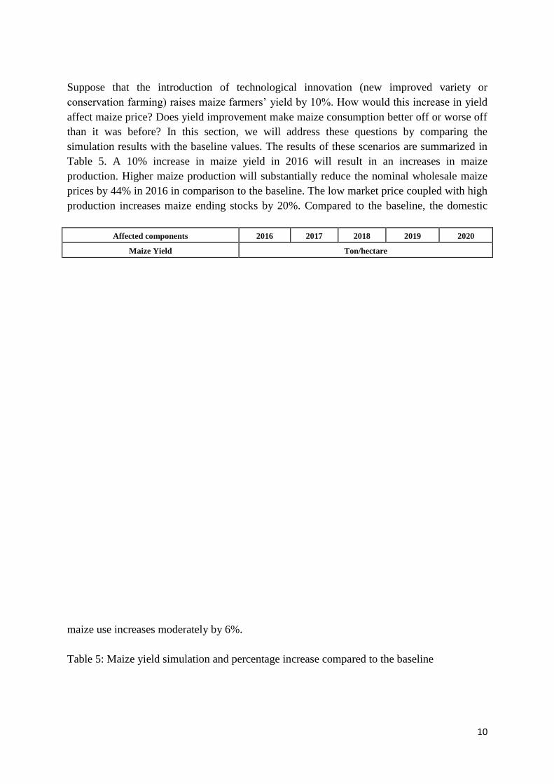
Suppose that the introduction of technological innovation (new improved variety or

conservation farming) raises maize farmers’ yield by 10%. How would this increase in yield

affect maize price? Does yield improvement make maize consumption better off or worse off

than it was before? In this section, we will address these questions by comparing the

simulation results with the baseline values. The results of these scenarios are summarized in

Table 5. A 10% increase in maize yield in 2016 will result in an increases in maize

production. Higher maize production will substantially reduce the nominal wholesale maize

prices by 44% in 2016 in comparison to the baseline. The low market price coupled with high

production increases maize ending stocks by 20%. Compared to the baseline, the domestic

maize use increases moderately by 6%.

Table 5: Maize yield simulation and percentage increase compared to the baseline

Affected components 2016 2017 2018 2019 2020

Maize Yield Ton/hectare

11

Source: Model output

4.3. Maize price leadership

The extended VAR procedure Toda and Yamamoto (1995) causality test employed to

analyse the lead-lag price relationships among regional wholesale maize markets. The

findings from Toda and Yamamoto causality test indicate that Addis Ababa maize market

price movement influences the surplus wholesale maize markets of Hosaena, Nekemete, and

Nazareth4. Likewise, Addis Ababa maize market price dictates maize price determination of

all deficit regional maize markets considered in this study. Therefore, the null hypothesis of

no causality from Addis Ababa maize price to the above-mentioned surplus and deficit maize

markets has been rejected. In the majority of cases, the direction of causation is

4 Unit root and Toda and Yamamoto causality test results are not reported here, but full results will be provided

upon request.

Baseline 2.80 2.84 2.88 2.90 2.92

Scenario 3.08 2.84 2.88 2.90 2.92

Absolute change 0.28 0.00 0.00 0.00 0.00

% Change 10% 0% 0% 0% 0%

Total Maize Production Thousand tonnes

Baseline 6532.77 6557.42 6583.7 6597.75 6634.74

Scenario 7186.05 6557.42 6583.7 6597.75 6634.74

Absolute change 653.28 0.00 0.00 0.00 0.00

% Change 10% 0% 0% 0% 0%

Domestic Maize Use Thousand tonnes

Baseline 6314.72 6579.81 6711.3 6778.54 6829.09

Scenario 6704.31 6722.15 6777.14 6808.81 6842.93

Absolute change 389.58 142.34 65.84 30.27 13.84

% Change 6% 2% 1% 0% 0%

Maize Ending stock Thousand tonnes

Baseline 1334.92 1312.53 1185 1004.17 809.807

Scenario 1598.61 1433.88 1240.47 1029.41 821.22

Absolute change 263.69 121.35 55.51 25.24 11.42

% Change 20% 9% 5% 3% 1%

Nominal Wholesale Maize Price ETB/ton

Baseline 4413.72 6137.31 8659.20 11795.20 15273.5

Scenario 2476.29 5400.31 8305.38 11626.83 15193.98

Absolute change -1937.42 737.00 353.80 -168.33 -79.49

% Change -44% -12% -4% -1% -1%

12

unidirectional from Addis Ababa price to the rest regional maize markets. The converse,

however, does not hold except for the deficit Dese maize market. Apart from this one case,

Addis Ababa maize price is exogenous to the rest regional maize markets. Thus, Addis

Ababa’s wholesale maize market is behaving like a dominant maize market in Ethiopia. The

geographical advantage enables Addis Ababa wholesale maize market to have large number

of feeder markets, which further contributes to unidirectional price influence.

4.4 Long-run relationships

Since the price series are non-stationary and integrated of the same order, cointegration

analysis is therefore appropriate to investigate the long-run relation among wholesale maize

market prices. Given the large number of maize markets, cointegration tests are conducted in

a pairwise fashion. Following the results of T-Y causality test, Addis Ababa maize market is

treated as exogenous maize market. Thus, in the subsequent cointegration analysis, regional

wholesale maize markets are paired with Addis Ababa maize market.

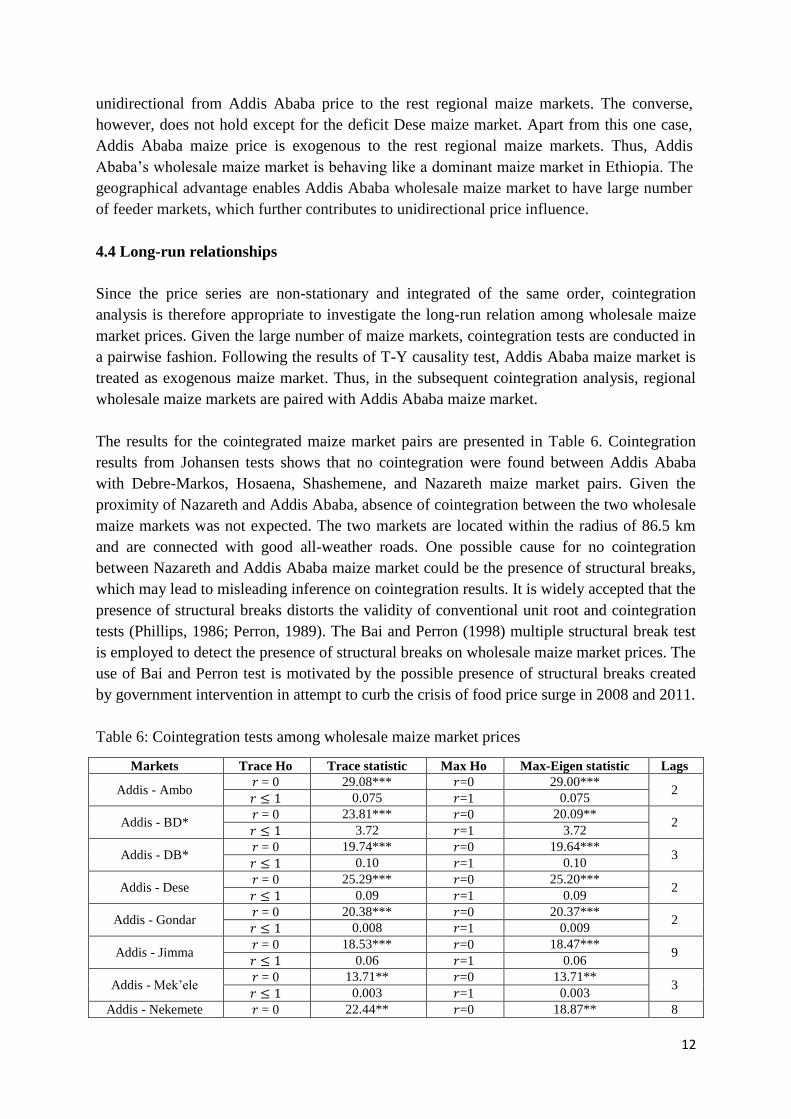
The results for the cointegrated maize market pairs are presented in Table 6. Cointegration

results from Johansen tests shows that no cointegration were found between Addis Ababa

with Debre-Markos, Hosaena, Shashemene, and Nazareth maize market pairs. Given the

proximity of Nazareth and Addis Ababa, absence of cointegration between the two wholesale

maize markets was not expected. The two markets are located within the radius of 86.5 km

and are connected with good all-weather roads. One possible cause for no cointegration

between Nazareth and Addis Ababa maize market could be the presence of structural breaks,

which may lead to misleading inference on cointegration results. It is widely accepted that the

presence of structural breaks distorts the validity of conventional unit root and cointegration

tests (Phillips, 1986; Perron, 1989). The Bai and Perron (1998) multiple structural break test

is employed to detect the presence of structural breaks on wholesale maize market prices. The

use of Bai and Perron test is motivated by the possible presence of structural breaks created

by government intervention in attempt to curb the crisis of food price surge in 2008 and 2011.

Table 6: Cointegration tests among wholesale maize market prices

Markets Trace Ho Trace statistic Max Ho Max-Eigen statistic Lags

Addis - Ambo 𝑟 = 0 29.08*** 𝑟=0 29.00***

2 𝑟 ≤ 1 0.075 𝑟=1 0.075

Addis - BD* 𝑟 = 0 23.81*** 𝑟=0 20.09**

2 𝑟 ≤ 1 3.72 𝑟=1 3.72

Addis - DB* 𝑟 = 0 19.74*** 𝑟=0 19.64***

3 𝑟 ≤ 1 0.10 𝑟=1 0.10

Addis - Dese 𝑟 = 0 25.29*** 𝑟=0 25.20***

2 𝑟 ≤ 1 0.09 𝑟=1 0.09

Addis - Gondar 𝑟 = 0 20.38*** 𝑟=0 20.37***

2 𝑟 ≤ 1 0.008 𝑟=1 0.009

Addis - Jimma 𝑟 = 0 18.53*** 𝑟=0 18.47***

9 𝑟 ≤ 1 0.06 𝑟=1 0.06

Addis - Mek’ele 𝑟 = 0 13.71** 𝑟=0 13.71**

3 𝑟 ≤ 1 0.003 𝑟=1 0.003

Addis - Nekemete 𝑟 = 0 22.44** 𝑟=0 18.87** 8

13

𝑟 ≤ 1 3.57 𝑟=1 3.57

Addis - Woliso 𝑟 = 0 35.06*** 𝑟=0 34.91***

2 𝑟 ≤ 1 0.15 𝑟=1 0.15

Addis - Ziway 𝑟 = 0 27.01*** 𝑟=0 26.87***

2 𝑟 ≤ 1 0.15 𝑟=1 0.15

*BD and DB stand for Bahir Dar and Debre-Birhan markets

***, ** significance level at 1 and 5%

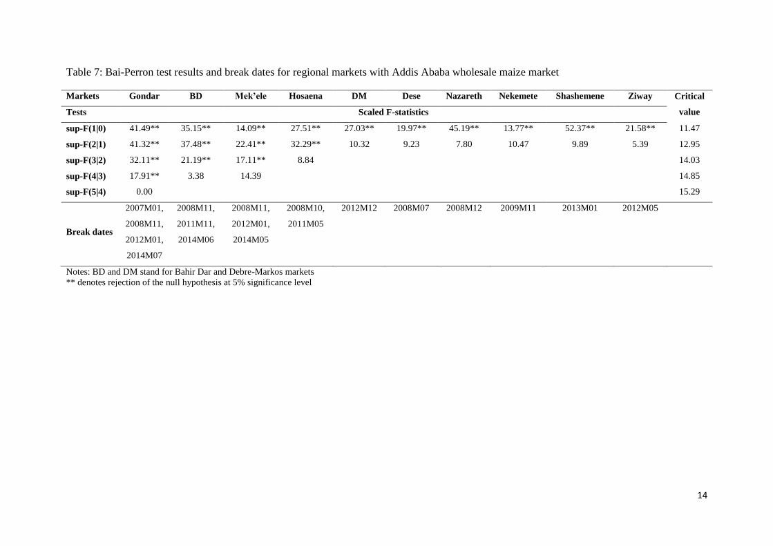
The results for structural breaks on wholesale maize market prices are presented in Table 7.

The sequential Bai and Perron test results identified 15 breakpoints. The 2008 M07, M10,

M11, and M12 structural breaks are likely associated with the Ethiopian government

macroeconomic intervention. In March 2008, the government restricted foreign exchange

access to private traders. The 2009, 2010, and 2012 breaks are perhaps the delayed effects of

global commodity price crisis of 2008 and 2011.

14

Table 7: Bai-Perron test results and break dates for regional markets with Addis Ababa wholesale maize market

Markets Gondar BD Mek’ele Hosaena DM Dese Nazareth Nekemete Shashemene Ziway Critical

value Tests Scaled F-statistics

sup-F(1|0) 41.49** 35.15** 14.09** 27.51** 27.03** 19.97** 45.19** 13.77** 52.37** 21.58** 11.47

sup-F(2|1) 41.32** 37.48** 22.41** 32.29** 10.32 9.23 7.80 10.47 9.89 5.39 12.95

sup-F(3|2) 32.11** 21.19** 17.11** 8.84 14.03

sup-F(4|3) 17.91** 3.38 14.39 14.85

sup-F(5|4) 0.00 15.29

Break dates

2007M01,

2008M11,

2012M01,

2014M07

2008M11,

2011M11,

2014M06

2008M11,

2012M01,

2014M05

2008M10,

2011M05

2012M12 2008M07 2008M12 2009M11 2013M01 2012M05

Notes: BD and DM stand for Bahir Dar and Debre-Markos markets

** denotes rejection of the null hypothesis at 5% significance level

15

In general, the results from the Bai and Perron test reveal that the presence of structural break

is evident in maize market prices and they might have an impact on cointegration test.

Therefore, it is important to retest cointegration among wholesale maize markets by

considering the effects of structural breaks. Following Rafailidis and Katrakilidis (2014), we

estimated the Dynamic Ordinary Least Square approach (DOLS) to investigate cointegration

test by incorporating the identified structural breaks in the form of dummy variables.

Analysing cointegration by taking into account breaks gives a different story for maize

markets considered as non-cointegrated in the Johansen’s approach (see tables 8 and 9).

Regional maize markets (Shashemene, Nazareth, Debre-Markos, and Hosaena) that are found

to have no-cointegration with Addis Ababa maize market have become cointegrated when

structural breaks are taken into account.

Table 8: DOLS estimation for Hosaena and Debre-Markos maize markets

Hosaena and Addis Ababa market pairs

Variables Coefficients t-Statistic

Panel A. Long run equilibrium results from DOLS

ADDIS_ABABA 1.15*** 44.53

Constant -21.61** -2.21

HOS08 -87.86* -1.75

HOS11 62.92 1.34

Adj. R2 0.95

Panel B: Cointegration test for the market pairs

Ut = -2.25**

Debre-Markos and Addis Ababa market pairs



Constant -35.64** -1.99

DM12 46.97 0.55

Adj. R2 0.94


Ut = -2.79***

Notes: Leads and lags specifications are based on AIC criterion

𝑈𝑡 is the innovation series obtained by dynamic ordinary least squares cointegration equation.

***, **, * denotes rejection of the null hypothesis at 1%, 5%, and 10% significance level

16

Table 9: DOLS estimation for Nazareth and Shashemene maize markets

Nazareth and Addis Ababa market pairs

Variables Coefficients t-Statistic



Constant -18.43 -1.53

NAZ08 40.48 0.68

Adj. R2 0.95


Ut = -2.47**

Shashemene and Addis Ababa market pairs



Constant -29.21 -1.65

SHASH13 159.75* 1.89

Adj. R2 0.92


Ut = -2.74**

Notes: Leads and lags specifications are based on AIC criterion

𝑈𝑡 is the innovation series obtained by dynamic ordinary least squares cointegration equation.

***, **, * denotes rejection of the null hypothesis at 1%, 5%, and 10% significance level

5. CONCLUSIONS

This study aimed at examining the price formation and dynamics in the Ethiopian maize

market. Furthermore, we empirically tested the central maize market hypothesis. Results from

the central market hypothesis test indicate that Addis Ababa wholesale maize market serves

as an important hub for maize market price formation, and more importantly as a hotspot for

source of maize price shocks, which influence the short and long-run price fluctuations of

regional maize markets. Spatial maize market cointegration tests were conducted by taking

into account structural breaks. Cointegration tests reveal that all regional maize markets

paired with the central market are cointegrated. The cointegration of all maize market pairs

considered in this study is a reflection of better spatial maize market linkages in Ethiopia

after the introduction of a Structural Adjustment Program (SAP).

17

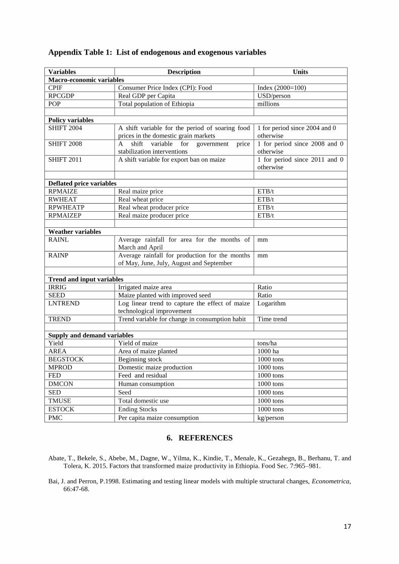
Appendix Table 1: List of endogenous and exogenous variables

Variables Description Units

Macro-economic variables

CPIF Consumer Price Index (CPI): Food Index (2000=100)

RPCGDP Real GDP per Capita USD/person

POP Total population of Ethiopia millions

Policy variables

SHIFT 2004 A shift variable for the period of soaring food

prices in the domestic grain markets

1 for period since 2004 and 0

otherwise

SHIFT 2008 A shift variable for government price

stabilization interventions

1 for period since 2008 and 0

otherwise

SHIFT 2011 A shift variable for export ban on maize 1 for period since 2011 and 0

otherwise

Deflated price variables

RPMAIZE Real maize price ETB/t

RWHEAT Real wheat price ETB/t

RPWHEATP Real wheat producer price ETB/t

RPMAIZEP Real maize producer price ETB/t

Weather variables

RAINL Average rainfall for area for the months of

March and April

mm

RAINP Average rainfall for production for the months

of May, June, July, August and September

mm

Trend and input variables

IRRIG Irrigated maize area Ratio

SEED Maize planted with improved seed Ratio

LNTREND Log linear trend to capture the effect of maize

technological improvement

Logarithm

TREND Trend variable for change in consumption habit Time trend

Supply and demand variables

Yield Yield of maize tons/ha

AREA Area of maize planted 1000 ha

BEGSTOCK Beginning stock 1000 tons

MPROD Domestic maize production 1000 tons

FED Feed and residual 1000 tons

DMCON Human consumption 1000 tons

SED Seed 1000 tons

TMUSE Total domestic use 1000 tons

ESTOCK Ending Stocks 1000 tons

PMC Per capita maize consumption kg/person

6. REFERENCES

Abate, T., Bekele, S., Abebe, M., Dagne, W., Yilma, K., Kindie, T., Menale, K., Gezahegn, B., Berhanu, T. and

Tolera, K. 2015. Factors that transformed maize productivity in Ethiopia. Food Sec. 7:965–981.

Bai, J. and Perron, P.1998. Estimating and testing linear models with multiple structural changes, Econometrica,

66:47-68.

18

Central Statistical Agency (CSA). 2011. Agricultural sample survey 2010/2011. Vol I. Report on area and

production of major crops (private peasant holdings, Meher season).

The Food and Agriculture Organization (FAO). 2015. FAOSTAT production database. Retrieved 05/11/2015,

http:/faostat3.fao.org/download.

Getnet, K., Verbeke, W. and Viaene, J. 2005. Modelling spatial price transmission in the grain markets of

Ethiopia with an application of ARDL approach to white teff. Agricultural Economics, 33:491-502.

Jaleta, M, and Gebermedhin, B. 2009. Price co-integration analyses of food crop markets: The case of wheat and

teff commodities in Northern Ethiopia. The International Association of Agricultural Economists

Conference, Beijing, China; August 16-22, 2009.

Johansen, S., 1991. Estimation and hypothesis testing of cointegration vectors in Gaussian vector autoregressive

models. Econometrica, 59(6):1551-1580.

Kelbore, Z.G., 2013. Transmission of world food prices to domestic market: The Ethiopian case. University of

Trento.

Negassa, A., R. Myers, and E Gabre-Madhin. 2004. Grain marketing policy changes and spatial efficiency of

maize and wheat markets in Ethiopia. International Food Policy Research Institute (IFPRI), MTDI

Discussion Paper 66.

Perron, P., 1989. The great crash, the oil price shock, and the unit root hypothesis, Econometrica, 57:1361-1401.

Phillips, P.C.B., 1986. Understanding spurious regression in econometrics, Journal of Econometrics, 33:311-

340.

Rafailidis, P., and Katrakilidis, C. 2014. The relationship between oil prices and stock prices: a non-linear

asymmetric cointegration approach, Applied Financial Economics, 24:793:800.

Regional Agricultural Trade Expansion Support Programme (RATES). 2003. Maize market assessment and

baseline study for Ethiopia, Nairobi, Kenya.

Tamru, S., 2013. Spatial integration of cereal markets in Ethiopia. Addis Ababa, Ethiopia: Ethiopia Strategy

Support Program - Ethiopian Development Research Institute.

Toda, H.Y., and Yamamoto, T. 1995. Statistical inference in vector auto-regressions with partially integrated

processes. J. Econ. 66:225–250.

Ulimwengu, J.M., Workneh, S. and Paulosm, Z. 2009. Impact of soaring food price in Ethiopia: does location

matter? IFPRI.

United States Department of Agriculture (USDA). 2015. Commodity database. Available:

http://apps.fas.usda.gov/psdonline/psdquery.aspx [2015, 24 November].

http://apps.fas.usda.gov/psdonline/psdquery.aspx

Modelling price formation and dynamics in the Ethiopian maize...

Documents

Transcript of Modelling price formation and dynamics in the Ethiopian maize...