Modelling of Non-Stationary Mobile RadioChannels Incorporating the Brownian Mobility

Model With DriftAlireza Borhani and Matthias Patzold

Abstract—This paper is a pioneering attempt to utilize aBrownian motion (BM) process with drift to model the mobileradio channel under non-stationary conditions. It is assumedthat the mobile station (MS) starts moving in a semi-randomway, but subject to follow a given direction. This movingscenario is modelled by a BM process with drift (BMD). Thestarting point of the movement is a fixed point in the two-dimensional (2D) propagation area, while its destination isa random point along a predetermined drift. To model thepropagation area, we propose a non-centred one-ring scatteringmodel in which the local scatterers are uniformly distributedon a ring that is not necessarily centred on the MS. Thesemi-random movement of the MS results in local angles-of-arrival (AOAs) and local angles-of-motion (AOMs), which arestochastic processes instead of random variables. We present thefirst-order density of the AOA and AOM processes in closedform. Subsequently, the local power spectral density (PSD) andautocorrelation function (ACF) of the complex channel gain areprovided. The analytical results are simulated, illustrated, andphysically explained. It turns out that the targeted Brownianpath model results in a statistically non-stationary channelmodel. The interdisciplinary idea of the paper opens a newperspective on the modelling of non-stationary channels underrealistic propagation conditions.

Index terms — Channel modelling, Brownian motion, non-stationary channels, local power spectral density, local autocor-relation function.

I. INTRODUCTION

TO develop mobile communication systems, geometricchannel models are recognized as one of the most

effective candidates, which allow a highly accurate systemperformance analysis. As an example, the one-ring scatteringmodel [1]–[3], in which the local scatterers are uniformlydistributed on a ring centered on the MS, is an appropri-ate model capturing the propagation effects in rural andsub-urban propagation areas. The unified disk scatteringmodel (UDSM) [4] is also one of the most general geo-metric channel models, which covers numerous circularly-symmetric scattering models as special cases, including theone-ring model. In this regard, an overview of the mostimportant geometric channel models can be found in [5].

Geometric channel models often profit from a commonsimplification, namely the stationarity assumption of thestochastic channel in time. Considering a very short obser-vation time instant justifies a time-invariant AOA at the MS,which then results in a statistically stationary channel model.Many empirical and analytical investigations, e.g., [6]–[8],

Manuscript received July 12, 2013; accepted August 1, 2013.A. Borhani and M. Patzold are with the Faculty of Engineering

and Science, University of Agder, 4898 Grimstad, Norway (e-mails:{alireza.borhani, matthias.paetzold}@uia.no).

however, show that this property is only valid for very shorttravelling distances [9]. This calls for the need to developand analyze stochastic channel models under non-stationaryconditions.

Despite the drastic number of investigations on stationarygeometric channel models, the literature lacks studies on non-stationary geometric channel models. Only a small numberof analytical studies, e.g., [10]–[13], cope with the statisticalproperties of non-stationary channels. To the best knowledgeof the authors, except the non-stationary one-ring scatteringmodel studied in [14], none of the established geometricscattering models listed in [5] has been analyzed undernon-stationary conditions. In [14], a non-stationary one-ringchannel model has been derived by assuming that the MSmoves from the center of the ring to the ring’s border ona straight line. In this paper, we further expand the ideaof [14] by allowing the MS to randomly fluctuate arounda straight line, where its starting point is not necessarily thering’s center. It can be any point inside the ring of scatterers.To this end, we let the MS move in a semi-random way, butsubject to follow a given preferred direction. By establishingan analogy between such a motion and the chaotic movementof particles suspended in fluids discovered by Robert Brown(see [15]), we model the travelling path of the MS by aBMD. We coin the term targeted Brownian path model toaddress the proposed path model of the MS. For a givenBM process, the randomness of the path can be controlledby a single parameter. By eliminating the randomness of thepath, the MS arrives at a fixed destination point via a straightpath. Accordingly, the path model of [14] can be obtained asa special case of the proposed targeted Brownian path model.

Moving along a targeted Brownian path results in localAOAs and local AOMs, which are modelled by stochasticprocesses rather than random variables. We present the first-order density of the AOA and AOM processes in closed form.Expressions for the local PSD of the Doppler frequenciesand ACF of the complex channel gain are also provided.Numerical computations at 2.1 GHz illustrate the analyticalresults and verify the non-stationarity of the channel model. Itis shown that non-stationarity in time contradicts the commonisotropic propagation assumption on the channel. It is alsoproved that the one-ring scattering model can be obtained asa special case of the proposed channel model of this paper.

It is worth mentioning that 3D BM processes have beenused to model fully random motions of mobile users [16].However, 1D BM processes with drift have never been usedto model semi-random motions of mobile users. Several othermobility models have also been employed in mobile ad hocnetworks [17], but not in the area of channel modelling. In a

Proceedings of the World Congress on Engineering and Computer Science 2013 Vol II WCECS 2013, 23-25 October, 2013, San Francisco, USA

ISBN: 978-988-19253-1-2 ISSN: 2078-0958 (Print); ISSN: 2078-0966 (Online)

WCECS 2013

nutshell, the novelty of this paper arises from the pioneeringutilization of the BMD process as a path model for themodelling of non-stationary mobile fading channels.

The remainder of this paper is organized as follows.Section II gives a brief introduction to BM processes asa physical phenomenon, while Section III utilizes the BMprocess for developing the targeted Brownian path model.Section IV describes the propagation scenario by meansof the non-centred one-ring scattering model. The complexchannel gain of the proposed channel model is then describedin Section V. Section VI investigates the statistical propertiesof the channel model. Numerical results are provided inSection VII. Finally, Section VIII summarizes our mainfindings and draws the conclusions.

II. PRINCIPLES OF THE BM PROCESS

BM was originally discovered in 1827 by the famousbotanist, Robert Brown. It describes the chaotic movementof particles suspended in a fluid or gas [15]. In the 1860s,there were experimentalists who clearly recognized that themotion is due to the impact of suspending molecules. Finally,in 1906, Albert Einstein [18] offered an exact physicalexplanation of such a motion based on the bombardment ofthe suspended particles by the atoms of the suspending fluid.In 1908, a mathematical explanation of the BM was providedby Langevin [19]1. BM processes have a wide range ofapplications, such as modelling of stock market fluctuations,medical imaging, and fractal theory [21]. In mobile adhoc networks, 2D BM processes (random walk) are alsoemployed to model irregular motions of mobile nodes [17].The model is then used for network layer analysis.

A stochastic process {B(t) : t ∈ [0, T ]} is said to be astandard BM process if:

1) B(0) = 0.2) ∀ 0 ≤ s < t ≤ T , the random variable given

by the increment B(t) − B(s) follows the Gaussiandistribution with zero mean and variance t − s, i.e.,B(t)−B(s) ∼ N(0, t− s).

3) ∀ 0 ≤ s < t < u < v ≤ T , the increments B(t)−B(s)and B(v)−B(u) are statistically independent.

From the conditions above, it can be concluded that B(t) is aWiener process with normally and independently distributedincrements.

III. PATH MODELLING

In what follows, we first provide an equivalent spatialrepresentation of the temporal BM process. Subsequently,the proposed local BM process is used to model the targetedmotion of the MS along a predetermined drift.

A. Spatial Representation of the BM Process

To establish an analogy between the BM process and theMS movement, let us first assume that the MS starts froma given point with Cartesian coordinates (xs, ys) in the 2Dplane. The aim is to model the random path starting from(xs, ys) via the BM process described in Section II. For thispurpose, we establish a mapping from the temporal represen-tation of the BM process B(t) to the spatial representation

1A translation of [19] into English has been provided in [20].

of the BM process B(x) by replacing the temporal variablet by the spatial variable x. Accordingly, the first conditionof the BM process, i.e., B(0) = 0, changes to B(xs) = 0.By assuming (xd, yd) as the terminal point of the movement,we introduce the scalar standard BM process over the range[xs, xd] by means of the spatial stochastic process B(x),which satisfies the following three conditions:

1) B(xs) = 0.2) ∀ xs ≤ xp < x ≤ xd, the random variable given

by the increment B(x)−B(xp) follows the Gaussiandistribution with zero mean and variance x− xp, i.e.,B(x)−B(xp) ∼ N(0, x− xp).

3) ∀ xs ≤ xp < x < xq < xm ≤ xd, the incrementsB(x) − B(xp) and B(xm) − B(xq) are statisticallyindependent.

For computational reasons, it is useful to consider the BMprocess at discrete values of x. To this end, we define∆x = (xd − xs)/L for some positive integer L. Hence,Bl = B(xl) denotes the BM process at xl = xs + l∆x (l =0, 1, ..., L). Now, with reference to Conditions 2 and 3, it canbe concluded that Bl = Bl−1+∆Bl, where each ∆Bl is anindependent normal distributed random variable of the formN(0,∆x).

B. The Targeted Brownian Path ModelTo model the targeted motion of the MS in the 2D plane,

we propose a path with a controllable drift in a preferreddirection, while the fluctuations of the path are modeled bythe spatial BM process Bl. Accordingly, the path P of theMS is modelled as follows

P :

{(xl, yl)

∣∣∣∣ xl = xs + l∆x,yl = axl + b+ σyBl,

}(1)

where l = 0, 1, ..., L is the position index, the variable adenotes the slope of the drift, b is a constant shift alongthe y-axis, and σy allows to control the randomness of thepath. Considering the fact that the randomness of the pathP originates inherently from the randomness of the BMprocess Bl, the parameter σy provides an additional degree offreedom to control the randomness. For instance, by settingσy to 0, any point on the line represented by yl = axl+b canbe reached. Whereas, increasing the value of σy reduces thechance of arriving at that point. However, the mean directionof the path remains unchanged. It is also noteworthy that thepath model in (1) reduces to that in [14] if σy = 0. Themodel also enables to incorporate random fluctuations onlyalong a specific line. For instance, by increasing a towardsinfinity, the fluctuations occur only along the y-axis. Thesame behaviour can be attained along any other line (axis)if we simply rotate the coordinate system.

In mobile communications, the proposed targeted Brow-nian path can be a very useful model to describe typicaldynamics of users in motion, such as persons walking alonga street, but not necessarily along a very smooth path. Invehicular communications, the model can also be used toexplain the jittery motion of the vehicle antenna, while thevehicle is moving along a given direction.

IV. THE PROPAGATION SCENARIO

To cope with the scattering effect caused by the prop-agation area, we propose a non-centred one-ring scattering

Proceedings of the World Congress on Engineering and Computer Science 2013 Vol II WCECS 2013, 23-25 October, 2013, San Francisco, USA

ISBN: 978-988-19253-1-2 ISSN: 2078-0958 (Print); ISSN: 2078-0966 (Online)

WCECS 2013

model, in which the local scatterers are uniformly distributedon a ring that is not necessarily centred on the MS. Thedisplacement of the MS from the ring’s center results in anon-isotropic channel model. This model is an appropriategeometric scattering model to explain environments, in whichthe base station (BS) antenna is highly elevated to scattering-free levels, while the MS antenna is surrounded by a largenumber of local scatterers. This situation occurs mostly inrural and sub-urban areas.

Fig. 1 shows the proposed non-centred one-ring scatteringmodel with the uniform distribution of the local scatterersSn (n = 1, 2, ..., N) on a ring of radius R centeredon the origin. In this regard, αS

n denotes the angle-of-scatterer (AOS) associated with the nth scatterer. At areference point in time t0, the MS starts its movement from(x0, y0) and tracks the path P to reach (xL, yL) at time tL.The position of the MS at time tl ∈ [t0, tL] is describedby Cartesian coordinates (xl, yl). It is also assumed that theMS is moving with a constant velocity vR in the directionindicated by the AOM αv[l]. Owing to high path loss, weassume that at time tl, a wave emitted from the BS reachesthe MS at the AOA αR

n [l] after a single bounce by thenth randomly distributed scatterer Sn located on the ring.A realization of the proposed Brownian path P in such ageometric scattering model is shown in Fig. 2, in which thestarting point (x0, y0) of the path is set to the ring’s center2.

The above mentioned propagation scenario is completelydifferent from the one-ring scattering model [1]–[3], in whichthe MS is located at the center of the ring, while its AOMis a deterministic variable. Therein, considering a very shortobservation time results in a stationary and isotropic channelmodel, while herein, the proposed path P justifies a non-stationary non-isotropic channel model. The proposed jitterypath model P is also different from the smooth path modelof [14]. Indeed, the random behavior of the AOM αv[l] (seeFig. 2) allows a much more flexible non-stationary channelmodel than the one proposed in [14]. In what follows, afterproviding an expression for the complex channel gain, westudy the statistical properties of the proposed non-stationarychannel model.

V. THE COMPLEX CHANNEL GAIN

The propagation scenario presented in Section IV is anon-stationary version of the typical fixed-to-mobile (F2M)scenario studied in [22, pp. 56–60]. Therein, the complexchannel gain µ(tl) of frequency-nonselective F2M channelswas modeled by means of a complex stochastic processrepresenting the sum of all scattered components as follows

µ(tl) = limN→∞

N∑n=1

cnej(2πfntl+θn). (2)

In the equation above, cn denotes the attenuation factorcaused by the physical interaction of the emitted wavewith the nth scatterer Sn, and fn stands for the Doppler

2We have chosen the ring’s center as the starting point of the movementto enable the verification of our numerical results (see Section VII) withthe ones from the one-ring scattering model. However, the analytical resultsprovided in the paper are not limited to such a special case.

y

xBS

R

][lRn

MS

nS

lx

ly][lv

S

n

Fig. 1. The non-centred one-ring scattering model for a single-bouncescattering scenario.

−300 −200 −100 0 100 200 300−300

−200

−100

0

100

200

300

X (m)

Y (

m)

Drift line

Starting point(xs, ys)

Terminal point(xd, yd)

Path PRing of scatterers

Fig. 2. Realization of a targeted Brownian path P in the ring of scatterers.The model parameters are L = 100, a = 1, b = 0, σy = 2, xs = 0m,xd = 150m, and R = 250m.

frequency3 caused by the movement of the MS. In addition,the random variable θn represents the phase shift of the nthpath, which is often assumed to be uniformly distributedbetween 0 and 2π [22, p. 59].

The complex channel gain in (2) suits the proposednon-stationary one-ring model, if we replace the Dopplerfrequency fn by fn(tl). This apparently minor change addsa great deal of mathematical computations to the statisticalcharacterization of the channel.

VI. STATISTICAL PROPERTIES OF THE CHANNEL

To investigate the statistical properties of the complexchannel gain described in (2), let us start from the local AOA,which plays a key role in other statistical quantities. Noticethat we defer the illustration and physical explanation of theanalytical results to Section VII.

3The frequency shift caused by the Doppler effect is given by f =fmax cos(α), where fmax = f0v/c0 is the maximum Doppler frequency,f0 denotes the carrier frequency, c0 stands for the speed of light, and αequals the difference between the AOA and the AOM [23].

Proceedings of the World Congress on Engineering and Computer Science 2013 Vol II WCECS 2013, 23-25 October, 2013, San Francisco, USA

ISBN: 978-988-19253-1-2 ISSN: 2078-0958 (Print); ISSN: 2078-0966 (Online)

WCECS 2013

A. The Local AOAs

Referring to the geometric scattering model in Fig. 1, theAOA αR

n [l] at the point (xl, yl) is given by

αRn [l] = arctan

(R sin(αS

n)− ylR cos(αS

n)− xl

). (3)

For a given position l, the only random variable in theright side of (3) is the AOS αS

n . Since the number N oflocal scatterers tends to infinity in the reference model, itis mathematically convenient to assume that the discreteAOS αS

n is a continues random variable αS , which isassumed to be uniformly distributed between −π and π (seeSection IV). By applying the concept of transformation ofrandom variables [24, p. 130] and performing some math-ematical manipulations, it can be shown that the first-orderdensity pαR(αR; l) of the stochastic process αR[l] in (3)becomes

pαR(αR;l)=1

2π

1− xl cos(αR) + yl sin(α

R)√R2 − (xl sin(αR)− yl cos(αR))

2

(4)

in which −π ≤ αR < π. It is worth mentioning thatpαR(αR; l) in (4) depends strongly on the position (xl, yl)of the MS. This means that the AOA αR[l] is not first-order stationary. As a special case, if the path P crosses thering’s center (0, 0), then pαR(αR; l) in (4) reduces to 1/(2π),which is the AOA probability density function (PDF) of theone-ring model [1]–[3].

B. The Local AOMs

By performing the linear interpolation scheme, the path Pbecomes continues and piecewise differentiable. This allowsus to present the AOM αv[l] at the location point (xl, yl) bythe following expression

αv[l] = arctan

(yl+1 − ylxl+1 − xl

)= arctan

(a+ σy

Bl+1 −Bl

xl+1 − xl

). (5)

In the right side of (5), Bl+1 − Bl is the only randomvariable, which follows the Gaussian distribution of theform N(0,∆x) (see Section III-A). Again, by applying theconcept of transformation of random variables, the PDFpαv (αv) of the AOM αv[l] in (5) is given by

pαv (αv) =1√

2πσ cos2(αv)e

−(tan(αv)−a)2

2σ2 (6)

where −π/2 ≤ αv ≤ π/2 and σ = σy/√∆x. Notice that

pαv (αv) in (6) is independent of the position (xl, yl) of theMS, meaning that the AOM αv is first-order stationary. Itcan be shown that the mean αv equals arctan(a), in whicha is the slope of the drift of the path P .

C. The Local PSD

Considering the local AOA αR[l] at the MS and the localAOM αv[l] of the MS, the local frequency shift f [l] causedby the Doppler effect is defined by the following expression

f [l] = fmax cos(αR[l]− αv[l]

)(7)

in which αR[l] and αv[l] are statistically described by thefirst-order density pαR(αR; l) in (4) and the PDF pαv (αv)in (6), respectively. The equation above is indeed a non-lineartransformation of the stochastic process α[l] = αR[l]−αv[l]to the stochastic process f [l]. Fixing the position index land applying again the concept of transformation of randomvariables results in the first-order density pf (f ; l) of thestochastic process f [l] presented in (8) [see the top of thenext page], in which pα,αv

(α, αv; l) is given in (9). Noticethat the Doppler frequency f in (8) varies between −fmax

and fmax.Following the same procedure provided in [22, p. 85], it

can be verified that the first-order density pf (f ; l) of theDoppler frequencies is directly proportional to the local PSDSµµ(f ; l) of the complex channel gain µ(tl), i.e.,

Sµµ(f ; l) = 2σ20pf (f ; l) (10)

where 2σ20 is the mean power of µ(tl) and pf (f ; l) is

provided in (8). If the path P goes through the ring’scenter (0, 0), the joint PDF pα,αv (α, αv; l) in (9) reduces topαv (αv)/(2π). Substituting this result in pf (f ; l) presentedin (8) and then multiplying the answer by the mean power2σ2

0 , gives the following local PSD

Sµµ(f ; l) =2σ2

0

πfmax

√1− (f/fmax)2

. (11)

The equation above represents the PSD of the one-ringscattering model, which is known as the Jakes PSD [23].Accordingly, the proposed channel model can locally meetthe one-ring scattering model.

D. The Local ACF

With reference to the generalized Wigner-Ville spec-trum [25, pp. 282-285], the local ACF rµµ(τ ; l) of thenon-stationary complex channel gain µ(tl) can be attainedby taking the inverse Fourier transform of the local PSDSµµ(f ; l) in (10). Accordingly, one can write

rµµ(τ ; l) =

fmax∫−fmax

Sµµ(f ; l)ej2πfτdf. (12)

As a special case, if the path P goes across the ring’s center,the local PSD Sµµ(f ; l) in (11) can be used to compute theinverse Fourier transform in (12). In this case, the local ACFrµµ(τ ; l) in (12) is simplified to 2σ2

0J0(2πfmaxτ), whereJ0(·) denotes the zeroth-order Bessel function of the firstkind [26, Eq. (8.411.1)].

VII. NUMERICAL RESULTS

Channel modelling at the 2 GHz band is of great impor-tance in mobile communications. With reference to the oper-ating frequency of the universal mobile telecommunicationssystem (UMTS), the carrier frequency f0 = 2.1GHz hasbeen chosen in our numerical computations. In addition, weconsider the path P shown in Fig. 2 as the travelling pathof the MS. This allows us to have the positions (xl, yl) forl = 0, 1, ..., L. It is also assumed that the MS is movingwith a velocity vR of 80 km/h, which results in a maximumDoppler frequency fmax of 155.5 Hz. The mean power 2σ2

0

has been set to unity.

Proceedings of the World Congress on Engineering and Computer Science 2013 Vol II WCECS 2013, 23-25 October, 2013, San Francisco, USA

ISBN: 978-988-19253-1-2 ISSN: 2078-0958 (Print); ISSN: 2078-0966 (Online)

WCECS 2013

pf (f ; l) =1

fmax

√1− (f/fmax)2

π/2∫−π/2

(pα,αv (arccos(f/fmax), αv) + pα,αv (− arccos(f/fmax), αv)

)dαv (8)

pα,αv (α, αv; l) =1

2π√2πσ cos2(αv)

∣∣∣∣∣∣1− xl cos(α+ αv) + yl sin(α+ αv)√R2 − (xl sin(α+ αv)− yl cos(α+ αv))

2

∣∣∣∣∣∣ e−(tan(αv)−a)2

2σ2 (9)

−20

2

0

50

1000

0.1

0.2

0.3

AOA, αR (rad)

Position, l

AO

AP

DF

,p

αR(α

R;l

)

Fig. 3. The behavior of the first-order density pαR (αR; l) in (4) for thepropagation scenario illustrated in Fig. 2.

Fig. 3 illustrates the first-order density pαR(αR; l) of theAOA process αR[l] provided in (4). With reference to thepath P shown in Fig. 2, the MS starts its movement from thecenter of the ring. This circularly symmetric starting pointexplains the uniform distribution of the AOA at l = 0. Bymoving along the path P , the probability of receiving signalsfrom the scatterers ahead reduces, whereas the probability ofreceiving from the scatterers behind increases. This behaviorcontinuous up to l = 100, where pαR(αR, 100) takes itsminimum value at αR = arctan(1) = 0.78 radian.

Fig. 4 displays the PDF pαv (αv) of the AOM αv[l] in (6).The simulated AOM is also shown in this figure. An excellentmatch between the simulation and analytical results can beobserved. The mean αv equals arctan(1) = 0.78 radian asshown in the figure. The plot shows explicitly the tendencyof the MS to follow the predetermined drift of the path P .This tendency depends solely on the slope a of the drift,which has been set to 1 herein. It is noteworthy that if therandomness σy of the path tends to zero, the AOM PDFapproaches the delta function at αv = 0.78 radian.

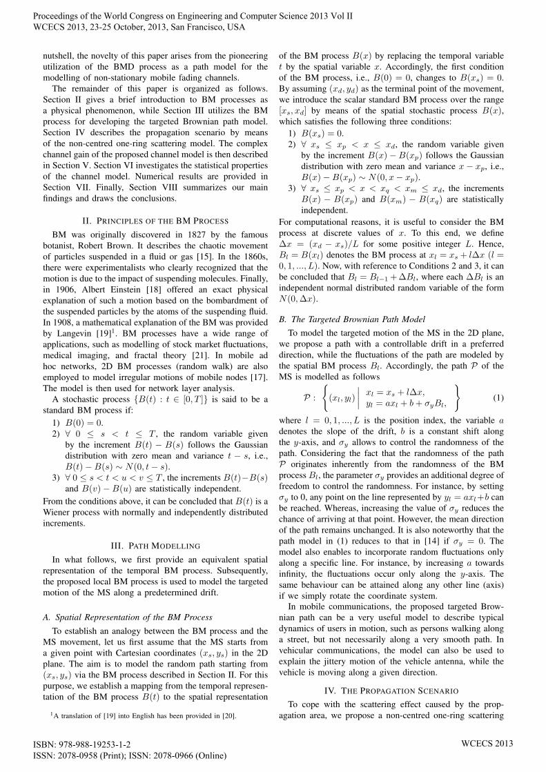
Fig. 5 depicts the local PSD Sµµ(f ; l) presented in (10).The classical Jakes PSD with a U-shape can be observedin the stationary case (l = 0), where the MS is located atthe ring’s center. At this position, Sµµ(f, 0) is a symmetricfunction with respect to f , indicating that the channel isinstantaneously isotropic. However, this feature does not holdif the MS continuous its motion along the path P . In thisregard, by increasing l, an asymmetric behavior of the localPSD Sµµ(f ; l) can be observed. Notice that moving alongthe path P results in confronting a lower number of scatterersahead and a higher number of them behind the MS. Thisallows a higher and a lower probability of negative and

−1 −0.5 0 0.5 10

0.2

0.4

0.6

0.8

1

1.2

AOM, αv (rad)A

OM

PD

F,p

αv(α

v)

SimulationAnalytical Mean line

αv = 0.78

Fig. 4. The behavior of the AOM PDF pαv (αv) in (6) for the propagationscenario illustrated in Fig. 2.

positive Doppler shifts as shown in Fig. 5.Fig. 4 displays the PDF pαv

(αv) of the AOM αv[l] in (6).The simulated AOM is also shown in this figure. An excellentmatch between the simulation and analytical results can beobserved. The mean αv equals arctan(1) = 0.78 radian asshown in the figure. The plot shows explicitly the tendencyof the MS to follow the predetermined drift of the path P .This tendency depends solely on the slope a of the drift,which has been set to 1 herein. It is noteworthy that if therandomness σy of the path tends to zero, the AOM PDFapproaches the delta function at αv = 0.78 radian.

Fig. 5 depicts the local PSD Sµµ(f ; l) presented in (10).The classical Jakes PSD with a U-shape can be observedin the stationary case (l = 0), where the MS is located atthe ring’s center. At this position, Sµµ(f, 0) is a symmetricfunction with respect to f , indicating that the channel isinstantaneously isotropic. However, this feature does not holdif the MS continuous its motion along the path P . In thisregard, by increasing l, an asymmetric behavior of the localPSD Sµµ(f ; l) can be observed. Notice that moving alongthe path P results in confronting a lower number of scatterersahead and a higher number of them behind the MS. Thisallows a higher and a lower probability of negative andpositive Doppler shifts as shown in Fig. 5.

Fig. 6 shows the absolute value of the local ACF rµµ(τ ; l)given in (12). Notice that due to the asymmetric behaviorof the PSD Sµµ(f ; l) (see Fig. 5), the ACF rµµ(τ ; l) is ingeneral complex. A quite time-varying behavior of the ACFcan be observed. It is also noteworthy that for a given timedifference τ = 0, the correlation increases through somefluctuations if l grows.

Proceedings of the World Congress on Engineering and Computer Science 2013 Vol II WCECS 2013, 23-25 October, 2013, San Francisco, USA

ISBN: 978-988-19253-1-2 ISSN: 2078-0958 (Print); ISSN: 2078-0966 (Online)

WCECS 2013

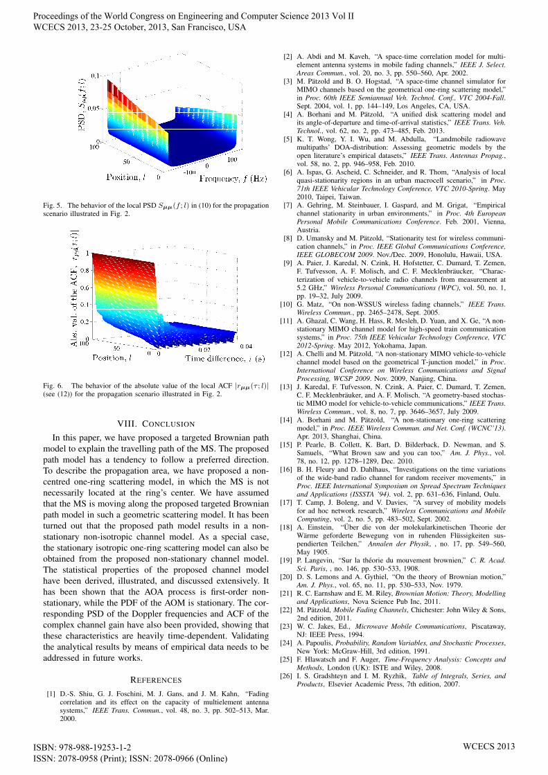
Fig. 5. The behavior of the local PSD Sµµ(f ; l) in (10) for the propagationscenario illustrated in Fig. 2.

Fig. 6. The behavior of the absolute value of the local ACF |rµµ(τ ; l)|(see (12)) for the propagation scenario illustrated in Fig. 2.

VIII. CONCLUSION

In this paper, we have proposed a targeted Brownian pathmodel to explain the travelling path of the MS. The proposedpath model has a tendency to follow a preferred direction.To describe the propagation area, we have proposed a non-centred one-ring scattering model, in which the MS is notnecessarily located at the ring’s center. We have assumedthat the MS is moving along the proposed targeted Brownianpath model in such a geometric scattering model. It has beenturned out that the proposed path model results in a non-stationary non-isotropic channel model. As a special case,the stationary isotropic one-ring scattering model can also beobtained from the proposed non-stationary channel model.The statistical properties of the proposed channel modelhave been derived, illustrated, and discussed extensively. Ithas been shown that the AOA process is first-order non-stationary, while the PDF of the AOM is stationary. The cor-responding PSD of the Doppler frequencies and ACF of thecomplex channel gain have also been provided, showing thatthese characteristics are heavily time-dependent. Validatingthe analytical results by means of empirical data needs to beaddressed in future works.

REFERENCES

[1] D.-S. Shiu, G. J. Foschini, M. J. Gans, and J. M. Kahn, “Fadingcorrelation and its effect on the capacity of multielement antennasystems,” IEEE Trans. Commun., vol. 48, no. 3, pp. 502–513, Mar.2000.

[2] A. Abdi and M. Kaveh, “A space-time correlation model for multi-element antenna systems in mobile fading channels,” IEEE J. Select.Areas Commun., vol. 20, no. 3, pp. 550–560, Apr. 2002.

[3] M. Patzold and B. O. Hogstad, “A space-time channel simulator forMIMO channels based on the geometrical one-ring scattering model,”in Proc. 60th IEEE Semiannual Veh. Technol. Conf., VTC 2004-Fall.Sept. 2004, vol. 1, pp. 144–149, Los Angeles, CA, USA.

[4] A. Borhani and M. Patzold, “A unified disk scattering model andits angle-of-departure and time-of-arrival statistics,” IEEE Trans. Veh.Technol., vol. 62, no. 2, pp. 473–485, Feb. 2013.

[5] K. T. Wong, Y. I. Wu, and M. Abdulla, “Landmobile radiowavemultipaths’ DOA-distribution: Assessing geometric models by theopen literature’s empirical datasets,” IEEE Trans. Antennas Propag.,vol. 58, no. 2, pp. 946–958, Feb. 2010.

[6] A. Ispas, G. Ascheid, C. Schneider, and R. Thom, “Analysis of localquasi-stationarity regions in an urban macrocell scenario,” in Proc.71th IEEE Vehicular Technology Conference, VTC 2010-Spring. May2010, Taipei, Taiwan.

[7] A. Gehring, M. Steinbauer, I. Gaspard, and M. Grigat, “Empiricalchannel stationarity in urban environments,” in Proc. 4th EuropeanPersonal Mobile Communications Conference. Feb. 2001, Vienna,Austria.

[8] D. Umansky and M. Patzold, “Stationarity test for wireless communi-cation channels,” in Proc. IEEE Global Communications Conference,IEEE GLOBECOM 2009. Nov./Dec. 2009, Honolulu, Hawaii, USA.

[9] A. Paier, J. Karedal, N. Czink, H. Hofstetter, C. Dumard, T. Zemen,F. Tufvesson, A. F. Molisch, and C. F. Mecklenbraucker, “Charac-terization of vehicle-to-vehicle radio channels from measurement at5.2 GHz,” Wireless Personal Communications (WPC), vol. 50, no. 1,pp. 19–32, July 2009.

[10] G. Matz, “On non-WSSUS wireless fading channels,” IEEE Trans.Wireless Commun., pp. 2465–2478, Sept. 2005.

[11] A. Ghazal, C. Wang, H. Hass, R. Mesleh, D. Yuan, and X. Ge, “A non-stationary MIMO channel model for high-speed train communicationsystems,” in Proc. 75th IEEE Vehicular Technology Conference, VTC2012-Spring. May 2012, Yokohama, Japan.

[12] A. Chelli and M. Patzold, “A non-stationary MIMO vehicle-to-vehiclechannel model based on the geometrical T-junction model,” in Proc.International Conference on Wireless Communications and SignalProcessing, WCSP 2009. Nov. 2009, Nanjing, China.

[13] J. Karedal, F. Tufvesson, N. Czink, A. Paier, C. Dumard, T. Zemen,C. F. Mecklenbrauker, and A. F. Molisch, “A geometry-based stochas-tic MIMO model for vehicle-to-vehicle communications,” IEEE Trans.Wireless Commun., vol. 8, no. 7, pp. 3646–3657, July 2009.

[14] A. Borhani and M. Patzold, “A non-stationary one-ring scatteringmodel,” in Proc. IEEE Wireless Commun. and Net. Conf. (WCNC’13).Apr. 2013, Shanghai, China.

[15] P. Pearle, B. Collett, K. Bart, D. Bilderback, D. Newman, and S.Samuels, “What Brown saw and you can too,” Am. J. Phys., vol.78, no. 12, pp. 1278–1289, Dec. 2010.

[16] B. H. Fleury and D. Dahlhaus, “Investigations on the time variationsof the wide-band radio channel for random receiver movements,” inProc. IEEE International Symposium on Spread Spectrum Techniquesand Applications (ISSSTA ’94). vol. 2, pp. 631–636, Finland, Oulu.

[17] T. Camp, J. Boleng, and V. Davies, “A survey of mobility modelsfor ad hoc network research,” Wireless Communications and MobileComputing, vol. 2, no. 5, pp. 483–502, Sept. 2002.

[18] A. Einstein, “Uber die von der molekularkinetischen Theorie derWarme geforderte Bewegung von in ruhenden Flussigkeiten sus-pendierten Teilchen,” Annalen der Physik, , no. 17, pp. 549–560,May 1905.

[19] P. Langevin, “Sur la theorie du mouvement brownien,” C. R. Acad.Sci. Paris, , no. 146, pp. 530–533, 1908.

[20] D. S. Lemons and A. Gythiel, “On the theory of Brownian motion,”Am. J. Phys., vol. 65, no. 11, pp. 530–533, Nov. 1979.

[21] R. C. Earnshaw and E. M. Riley, Brownian Motion: Theory, Modellingand Applications, Nova Science Pub Inc, 2011.

[22] M. Patzold, Mobile Fading Channels, Chichester: John Wiley & Sons,2nd edition, 2011.

[23] W. C. Jakes, Ed., Microwave Mobile Communications, Piscataway,NJ: IEEE Press, 1994.

[24] A. Papoulis, Probability, Random Variables, and Stochastic Processes,New York: McGraw-Hill, 3rd edition, 1991.

[25] F. Hlawatsch and F. Auger, Time-Frequency Analysis: Concepts andMethods, London (UK): ISTE and Wiley, 2008.

[26] I. S. Gradshteyn and I. M. Ryzhik, Table of Integrals, Series, andProducts, Elsevier Academic Press, 7th edition, 2007.

Proceedings of the World Congress on Engineering and Computer Science 2013 Vol II WCECS 2013, 23-25 October, 2013, San Francisco, USA

ISBN: 978-988-19253-1-2 ISSN: 2078-0958 (Print); ISSN: 2078-0966 (Online)

WCECS 2013