
Modelling of Multi-terminal VSC-HVDC Links for Power Flows ...
144
Luis Miguel Castro González Modelling of Multi-terminal VSC-HVDC Links for Power Flows and Dynamic Simulations of AC/DC Power Networks Julkaisu 1445 • Publication 1445 Tampere 2016
Transcript of Modelling of Multi-terminal VSC-HVDC Links for Power Flows ...

Luis Miguel Castro GonzálezModelling of Multi-terminal VSC-HVDC Links for Power Flowsand Dynamic Simulations of AC/DC Power Networks
Julkaisu 1445 • Publication 1445
Tampere 2016

Tampereen teknillinen yliopisto. Julkaisu 1445 Tampere University of Technology. Publication 1445
Luis Miguel Castro González
Modelling of Multi-terminal VSC-HVDC Links for Power
Flows and Dynamic Simulations of AC/DC Power Networks Thesis for the degree of Doctor of Science in Technology to be presented with due permission for public examination and criticism in Sähkötalo Building, Auditorium S2, at Tampere University of Technology, on the 5th of December 2016, at 12 noon.
Tampereen teknillinen yliopisto - Tampere University of Technology Tampere 2016

ISBN 978-952-15-3866-7 (printed) ISBN 978-952-15-3869-8 (PDF) ISSN 1459-2045

iii
Abstract
Power transmission systems are expanded in order to supply electrical energy to remote users, to
strengthen their operational security and reliability and to be able to carry out commercial
transactions with neighbouring power grids. Power networks successfully expand, at any time, by
incorporating the latest technological developments. A case in point is the current growth of
electrical power grids, in terms of both infrastructure and operational complexity, to meet an
unprecedented upward trend in global demand for electricity. Today’s expansion of the power grid
is being supported, more and more, by power electronics, in the form of flexible AC transmission
systems and HVDC systems using voltage-sourced converters. The latter option, in particular, has
been developing exceedingly rapidly since 1999, when the first commercial VSC-HVDC
transmission installation was commissioned; the voltage-sourced converter technology has
become the preferred option for transporting electricity when natural barriers are present (e.g. the
sea), in Europe and further afield. At least one influential European body has recommended that
the next step in the construction of the so-called European super grid, be a meshed HVDC
transmission system based on the use of the VSC technology, to facilitate further the massive
incorporation of renewable energy sources into the Pan European electrical grid, the harvesting of
hydrocarbons that lie in deep sea waters and the energy trading between neighbouring countries.
It is in this context that this thesis contributes new knowledge to the modelling of VSC-based
equipment and systems for the assessment of steady-state and transient stability analyses of
AC/DC power networks. The STATCOM, the back-to-back VSC-HVDC link, the point-to-point
VSC-HVDC link and the multi-terminal VSC-HVDC link, all receive research attention in this work.
The new models emanating from this research capture all the key steady-state and dynamic
characteristics of the equipment and network. This has required a paradigm shift in which the VSC
equipment has been modelled, here-to-fore, assuming that a voltage-sourced converter behaves
like an idealised voltage source. In contrast, the models developed in this research resort to an
array of basic power systems elements, such as a phase-shifting transformer and an equivalent
shunt susceptance, giving rise to a two-port circuit where the AC and DC sides of the VSCs are
explicitly represented. The ensuing VSC model is fundamentally different from the voltage source
model; it represents, in an aggregated manner, the array of semiconductor switches in the
converter and its PWM control. The VSC model was used as the basic building block with which to
develop all the VSC-based devices put forward in this thesis. The ultimate device is the multi-
terminal VSC-HVDC system, which may comprise an arbitrary number of VSC units
commensurate with the number of otherwise independent AC sub-networks and a DC network of
an arbitrary topology. The steady-state and dynamic simulations of the AC/DC systems are carried
out using a unified frame-of-reference which is amenable to the Newton-Raphson algorithm. This
framework accommodates, quite naturally, the set of discretised differential equations arising from
the synchronous generators, HVDC and FACTS equipment, and the algebraic equations
describing the conventional transmission lines, transformers and loads of the AC sub-networks.
The application areas covered in this work are: power-flow studies and dynamic simulations.

iv
Preface
Completion of this doctoral thesis was possible due to the help and support of several people. I
would like to express my sincere gratitude to all of them.
The research work presented in this thesis was carried out at the Department of Electrical En-
gineering (DEE), at Tampere University of Technology (TUT), to which I thank for having accepted
me to be part of its vibrant academic atmosphere, first as a visiting student and then as a PhD stu-
dent.
I am deeply grateful to Prof. Enrique Acha to whom I thank for supervising my thesis, providing
me always with his enormous expertise and due guidance throughout my research. I would like to
recognize that the years I spent in Finland under his supervision were the most fruitful in terms of
my professional growth. I thank him for having facilitated my research in Finland with his uncondi-
tional support and friendship. I would like to also thank Prof. Seppo Valkealahti for having accepted
me a visiting student when he was the Head of Department of Electrical Engineering.
I am grateful to Prof. Ali Abur and Prof. Neville R. Watson for examining my manuscript and
for providing me valuable comments which, undoubtedly, helped improve the quality of this thesis.
The staff of the DEE deserves my regards for providing me with valuable assistance in practi-
cal matters of the workplace.
I thank all the colleagues and friends that I encounter by chance in Tampere for their support
and friendship, especially thanking Luis Enrique, Carlos, Jorge Paredes, Rodolfo, Angélica, Mafer,
Moramay, Viri, Oscar, Kalle, Gabriel, Josmar, Victor, René, Rosa, Gaby, Pancho, Jan Servotte,
Nemät Dehghani, Andrii and many others with whom I spent unforgettable moments.
Last but not least, I express my most profound gratitude to my parents, Luis and Guadalupe,
and my siblings, Lupita, Victor, Leonardo and Cesar for their all-important encouraging words dur-
ing the time I spent in Finland.
México City, November 2016
Luis Miguel Castro González
v
Contents
Abstract…………………………………………………………………………………………………...… iii
Preface………………………………………………………………………………………………….……iv
Contents…………………………………………………………………………………………………...…v
List of figures……………………………………………………………………………………….………vii
List of tables…………………………………………………………………………………………………x
List of symbols and abbreviations………………………………………………………………………..xi
1 INTRODUCTION ........................................................................................................................ 1
1.1 Objectives and scientific contribution .................................................................................... 3
1.2 List of published papers ......................................................................................................... 4
1.3 Thesis outline ......................................................................................................................... 5
2 STATE-OF-THE-ART OF THE THESIS .................................................................................... 7
2.1 Early attempts to modelling VSC-based equipment for power systems simulations ........... 8
2.2 Advances in the state-of-the-art modelling of VSC-based equipment for power systems simulations ........................................................................................................................... 12
3 MODELLING OF VSC-BASED EQUIPMENT FOR POWER FLOWS.................................... 15
3.1 Voltage source converter model.......................................................................................... 16
3.2 On-load tap-changing transformer model ........................................................................... 19
3.3 STATCOM model ................................................................................................................ 20
3.3.1 Checking of the converter’s operating limits and nonregulated solutions ................. 22
3.3.2 Initialisation of variables ............................................................................................. 23
3.4 High-voltage direct current link ............................................................................................ 23
3.4.1 Point-to-point HVDC link model with DC power regulation capabilities .................... 27
3.4.2 Point-to-point HVDC link model feeding into a passive network ............................... 30
3.4.3 Back-to-back HVDC model ........................................................................................ 33
3.5 Multi-terminal VSC-HVDC links ........................................................................................... 34
3.5.1 Three-terminal VSC-HVDC link model ...................................................................... 36
3.5.2 Multi-terminal VSC-HVDC link model ........................................................................ 43
3.5.3 Unified solutions of AC/DC networks ......................................................................... 45
3.6 Conclusions ......................................................................................................................... 47
4 MODELLING OF VSC-BASED EQUIPMENT FOR DYNAMIC SIMULATIONS ..................... 49
4.1 STATCOM model for dynamic simulations ......................................................................... 50
4.2 VSC-HVDC models for dynamic simulations ...................................................................... 56
vi
4.2.1 VSC-HVDC dynamic model with DC power regulation capabilities .......................... 60
4.2.2 VSC-HVDC dynamic model with frequency regulation capabilities .......................... 65
4.3 Multi-terminal VSC-HVDC systems for dynamic simulations ............................................. 70
4.3.1 Three-terminal VSC-HVDC dynamic model .............................................................. 71
4.3.2 Multi-terminal VSC-HVDC dynamic model ................................................................ 81
4.4 Conclusions ......................................................................................................................... 85
5 CASE STUDIES ....................................................................................................................... 86
5.1 Power systems simulations including STATCOMs ............................................................. 86
5.1.1 New England 39-bus network, 2 STATCOMs ........................................................... 86
5.2 Point-to-point VSC-HVDC-upgraded power systems ......................................................... 96
5.2.1 Validation of the VSC-HVDC model for power regulation ......................................... 96
5.2.2 New England 39-bus network, 1 embedded VSC-HVDC link ................................. 100
5.2.3 Validation of the VSC-HVDC model providing frequency regulation ...................... 105
5.2.4 VSC-HVDC link feeding into low-inertia AC networks ............................................. 107
5.3 Multi-terminal VSC-HVDC-upgraded power systems ....................................................... 112
5.3.1 Validation of the multi-terminal VSC-HVDC dynamic model ................................... 112
5.3.2 Multi-terminal VSC-HVDC link with a DC ring ......................................................... 115
5.4 Conclusions ....................................................................................................................... 119
6 GENERAL CONCLUSIONS AND FUTURE RESEARCH WORK ........................................ 121
6.1 General conclusions .......................................................................................................... 121
6.2 Future research work ......................................................................................................... 123
REFERENCES................................................................................................................................. 125

vii
List of Figures
Figure 3.1 (a)STATCOM schematic representation; (b) VSC steady-state equivalent circuit ....... 16
Figure 3.2 Simplified representation of the power-flow model for the OLTC transformer; (a) Tap in nominal position, (b) Tap in off-nominal position............................................................................... 19
Figure 3.3 VSC-HVDC schematic representation ........................................................................... 23
Figure 3.4 Steady-state equivalent circuit of the VSC-HVDC link .................................................. 25
Figure 3.5 Multi-terminal VSC-HVDC system interconnecting power networks of various kinds .. 35
Figure 3.6 Steady-state equivalent circuit of a three-terminal VSC-HVDC link .............................. 36
Figure 3.7 Flow diagram of a true unified solution of the multi-terminal VSC-HVDC system ........ 47
Figure 4.1 Schematic diagram of the STATCOM and its control variables .................................... 51
Figure 4.2 DC voltage controller of the VSC ................................................................................... 52
Figure 4.3 DC power controller for the DC side of the VSC............................................................ 53
Figure 4.4 AC-bus voltage controller of the VSC ............................................................................ 53
Figure 4.5 Schematic representation of the VSC-HVDC link and its control variables .................. 57
Figure 4.6 DC voltage dynamic controller of the VSC-HVDC link .................................................. 58
Figure 4.7 DC-power controller of the VSC-HVDC link model ........................................................ 59
Figure 4.8 AC-bus voltage controllers: (a) rectifier station and (b) inverter station ........................ 60
Figure 4.9 Frequency controller of the VSC-HVDC link .................................................................. 67
Figure 4.10 Full VSC station with ancillary elements ...................................................................... 71
Figure 4.11 Representation of a three-terminal VSC-HVDC link and its control variables ............ 72
Figure 4.12 DC voltage dynamic controller of the slack converter VSCSlack ................................... 73
Figure 4.13 (a) DC-power controller of the converter of type VSCPsch and (b) Frequency controller of the converter of type VSCPass ........................................................................................................ 74
Figure 4.14 Modulation index controllers of the three converter stations making up the three-terminal HVDC system....................................................................................................................... 74
Figure 5.1 New England test system with two embedded STATCOMs ......................................... 87
Figure 5.2 Angular speed of the synchronous generators .............................................................. 89
Figure 5.3 Active power flow behaviour in some transmission lines............................................... 89
Figure 5.4 Reactive power flow behaviour in some transmission lines .......................................... 90
Figure 5.5 Voltage performance at different nodes of the network ................................................. 90
Figure 5.6 Reactive power generated by the STATCOMs.............................................................. 91
Figure 5.7 Voltage performance at the AC nodes of the VSCs ...................................................... 91
Figure 5.8 Voltage performance at several nodes of the network including two STATCOMs ....... 91
Figure 5.9 STATCOMs DC-bus voltages ........................................................................................ 92
Figure 5.10 STATCOMs DC current ................................................................................................ 92
Figure 5.11 Dynamic performance of the angle of the VSCs .................................................... 93

viii
Figure 5.12 Total active power losses incurred by the STATCOMs ............................................... 93
Figure 5.13 Dynamic behaviour of the modulation index of the STATCOMs ................................. 94
Figure 5.14 Performance of the DC voltages for different ratings of the capacitors....................... 95
Figure 5.15 Performance of the modulation ratio for different ratings of the capacitors ................ 95
Figure 5.16 Reactive power generation for different ratings of the capacitors ............................... 95
Figure 5.17 Test system used to validate the proposed VSC-HVDC model .................................. 96
Figure 5.18 DC voltage performance for the proposed and Simulink models ................................ 97
Figure 5.19 DC power performance for the proposed and Simulink models .................................. 98
Figure 5.20 Modulation indices performance for the proposed and Simulink models.................... 99
Figure 5.21 New England test system with embedded VSC-HVDC link ...................................... 101
Figure 5.22 Voltage performance at different nodes of the network ............................................. 102
Figure 5.23 Dynamic behaviour of the modulation indices ........................................................... 103
Figure 5.24 Reactive power generated by the VSCs of the HVDC link ........................................ 103
Figure 5.25 DC current behaviour of the rectifier and inverter ...................................................... 104
Figure 5.26 DC voltage behaviour of the VSC-HVDC system ...................................................... 104
Figure 5.27 AC active powers and DC power behaviour of the HVDC link .................................. 105
Figure 5.28 Dynamic performance of the various angles involved in the HVDC link ................... 105
Figure 5.29 Dynamic behaviour of the frequency at the inverter’s AC terminal and DC power: (a) Simulink model; (b) Proposed model .............................................................................................. 106
Figure 5.30 Dynamic performance of the DC voltages and modulation indices: (a) Simulink model; (b) Proposed model ......................................................................................................................... 107
Figure 5.31 VSC-HVDC link feeding into a low-inertia network .................................................... 108
Figure 5.32 Voltage behaviour in the low-inertia network ............................................................. 109
Figure 5.33 Frequency behaviour in the low-inertia network ........................................................ 109
Figure 5.34 Dynamic performance of the AC and DC powers of the HVDC link.......................... 110
Figure 5.35 Dynamic performance of R and dcII ......................................................................... 110
Figure 5.36 Dynamic performance of the DC voltages and modulation indices........................... 111
Figure 5.37 Frequency in the low-inertia network and DC voltage of the inverter for different gains of the frequency control loop ........................................................................................................... 112
Figure 5.38 Three-terminal VSC-HVDC link used to carry out the validation test ........................ 113
Figure 5.39 DC voltages of the VSCs comprising the three-terminal VSC-HVDC link. (a) Simulink model; (b) Developed model............................................................................................................ 114
Figure 5.40 DC power behaviour at the DC bus of the three VSCs. (a) Simulink model, (b) Developed model ............................................................................................................................. 114
Figure 5.41 Modulation ratio of the three VSCs. (a) Simulink model; (b) Developed model........ 115
Figure 5.42 Schematic representation of a multi-terminal VSC-HVDC link with a DC ring .......... 116
Figure 5.43 Converter’s DC voltage and power flows in the DC grid ........................................... 119
ix
Figure 5.44 Modulation ratio of the VSCs and frequency of the passive networks fed by VSCb, VSCd, VSCf....................................................................................................................................... 119

x
List of Tables Table 3.1 Types of VSCs and their control variables ....................................................................... 38
Table 5.1 Parameters of the STATCOMs ......................................................................................... 87
Table 5.2 STATCOM results as furnished by the power-flow solution ............................................. 88
Table 5.3 Initial values of the STATCOM variables for the dynamic simulation .............................. 88
Table 5.4 Parameters of the VSC-HVDC link ................................................................................... 97
Table 5.5 VSC-HVDC variables for the proposed model and Simulink model ................................ 99
Table 5.6 Parameters of the embedded VSC-HVDC link ............................................................... 100
Table 5.7 VSC-HVDC results given by the power-flow solution ..................................................... 101
Table 5.8 Initial values of the STATCOM variables for the dynamic simulation ............................ 102
Table 5.9 Parameters of the VSC-HVDC link with frequency regulation capabilities .................... 106
Table 5.10 Parameters of the VSC-HVDC link feeding into a low-inertia network ........................ 108
Table 5.11 VSC-HVDC results given by the power-flow solution ................................................... 109
Table 5.12 Different gain values for the frequency controller ......................................................... 111
Table 5.13 Parameters of the three-terminal VSC-HVDC link ....................................................... 113
Table 5.13 Parameters of the VSCs, AC1, AC3, AC5 and DC networks ......................................... 116
Table 5.14 State variables solution for each VSC .......................................................................... 117
Table 5.15 Voltages and injected powers at the AC networks ....................................................... 118
Table 5.16 Power flows in the DC ring............................................................................................ 118

xi
List of Symbols and Abbreviations
,V : Phase angle and magnitude of nodal voltages
gP , gQ : Generated active and reactive powers
d kP , dkQ : Active and reactive powers drawn by the load at bus k
calkP ,
calkQ : Active and reactive power injections at bus k
eqB : Equivalent shunt susceptance of the converter
dcC : DC capacitor of the converter
cH : Inertia constant of the converter’s DC capacitor
dcE : DC bus voltage
am : Modulation ratio of the converter
: Phase-shifting angle of the converter
swG : Conductance for computing the switching losses of the converter
,R X : Series resistance and reactance of the converter
,ltc ltcR X : Series resistance and reactance of the OLTC transformer
, ,f f fR X B : Resistance, reactance and susceptance of the AC filter of the converter
,dc dcG R : Conductance and resistance of the DC links
nomI : Nominal current of the converter
nomS : Rated apparent power of the converter
AC/DC: Alternating current/Direct current
EMTS: Electromagnetic transient simulation
IGBT: Insulated gate bipolar transistors
J : Jacobian matrix
HVDC: High-voltage direct current
OLTC: On-load tap changer
PWM: Pulse-width modulation
RMS: Root mean square
STATCOM: Static synchronous compensator
SVC: Static VAR compensator
VSC: Voltage source converter


1
1 Introduction
Population growth and its migration to already large metropolitan areas, continue apace. To avoid
the collapse of entire megalopolis in various parts of the world, the use of advanced technology
has become essential. In particular, technology driven by electricity has enabled large number of
people around the globe to reach higher levels of comfort, enabling more sophisticated human
activities. All this is coming with a heavy price tag on the use of natural resources, gas emissions
into the atmosphere beyond what it is deemed sustainable, toxic waste into the sea, deforestation
an open mining of large tracts of land in the quest for metals and hydrocarbons. All this activity is
clearly non-sustainable and modern society requires a paradigm shifts so that the new challenges
are adequately resolved.
Concerning the remit of this work, electrical power networks have been subjected to a relentless
expansion in order to meet the spiralling demand for electricity. This has brought great many chal-
lenges to the electricity supply industry as a whole. A case in point is the need to maintain the op-
erational integrity of the system in the face of a large penetration of renewable energy sources and
the widespread incorporation of power electronics equipment into the power grid to make it elec-
tronically controllable. Most of the so-called renewable energy sources of electricity use primary
energy resources that exhibit important degrees of randomness and use power electronics to
make them amenable to their incorporation into the power grid. This has led to a more flexible
electrical power grid but also one where the operational complexity has increased by a degree. All
this comes at a time when large tracts of the electrical power grid have aged and are up for renew-
al, such as transmission lines, transformers, generators and protection equipment. All this infra-
structure is critical to the well-being of an electrical power grid that would be “fit for purpose” to
satisfy the users’ expectations for the delivery of high quality electricity at their points of connection.
The fulfilment of such high expectations would require the incorporation of cutting-edge technology
and operating practises and tools. The aim would be to enable the supply of electrical energy at a
reasonable cost, with low power losses in the distribution and bulk power transmission systems,
bearing in mind reliability of supply and energy efficiency as the key drivers. In parallel with the
2
renewal of the critical infrastructure, the development of state-of-the-art models of the emerging
electrical equipment, control methods and simulation tools, requires continuous global effort.
These present and future developments would provide the theoretical foundations upon which the
new, smarter power grids will be built. It is argued in this research work, that power systems simu-
lation tools such as power flows and time-domain simulations would turn out to be the instrumental
tools that will assist in the decision-making process at the design, planning and operation stages of
future power grids.
The use of power electronic devices to enable a more flexible power grid aimed at achieving
higher throughputs and enhancing system stability are high on the agenda in many countries
around the globe; specifically, through the use of voltage source converters. The latest innovations
in the power electronics field in terms of semiconductor valves, bridges and control strategies are
motivating manufacturers to launch new converter designs into the global market, opening the
gates to a flurry of new applications. With more power electronics than ever before embedded into
the power system, a great deal of both technology and modelling issues are yet to be resolved. In
the particular field of power converter modelling, for utility-scale power systems simulations, there
has been a very creditable effort. However, it is often said that a voltage-sourced converter (VSC),
including its derived family of equipment (e.g., VSC-HVDC), operates according to the basic prin-
ciples of a controllable voltage source. It is argued here that this may be so only from a superficial
standpoint, applicable only to power system studies of limited scope. A deeper analysis of this grid-
connected equipment leads to the conclusion that they are very rich in dynamics, whose calcula-
tion success cannot always be guaranteed, if the underrepresented idealised voltage source con-
cept is used. Hence, one would need to resort to application tools which model the VSC at the in-
dividual valve-level, such as PSCAD-EMTDC, the SimPowerSystems block set within Simulink or,
alternatively, the new type of representations put forward in this research; each with their ad-
vantages and disadvantages.
This research work advances the topic of grid-connected VSC-based equipment modelling
aimed at the steady-state and dynamic simulations of power systems. The modelling of STAT-
COMs, back-to-back HVDC links, point-to-point HVDC links and multi-terminal HVDC systems are
all addressed here. These models have been developed bearing in mind the key operational char-
acteristics of the VSC-based equipment which will impact directly on the operation of the connect-
ed power grids. The encapsulation of the equipment’s key dynamic effects and efficient numerical
solutions of the ensuing models in terms of accuracy and computing times for steady-state and
dynamic analyses, have been issues of paramount importance. The family of models of high-
voltage, high-power VSC-based equipment which are introduced in this thesis, signify a paradigm
shift in the way this equipment has traditionally been modelled with respect to their fundamental
frequency, positive-sequence representation of their AC circuits. It ought to be remarked that these
models depart from the widely-adopted modelling practice of representing the VSC as idealised

3
voltage or current sources. It is confirmed in this research work, using credible “what if scenarios”
that these lumped models retain the key dynamics characteristics of the equipment by comparing
their responses against the switching-based models available in the SimPowerSystems block set
of Simulink. The STATCOM and the back-to-back, point-to-point and multi-terminal HVDC systems
using VSCs, all received research attention.
1.1 Objectives and scientific contribution
The main objective of this thesis is to advance the fundamental-frequency, positive-sequence
modelling, at their AC side, of the STATCOM, back-to-back HVDC link, point-to-point HVDC link
and multi-terminal HVDC systems suitable for power systems simulations, with reference to their
steady-state and dynamic operating regimes. Furthermore, a new frame-of-reference has been put
forward in order to accommodate, in a unified manner, the new models and the positive-sequence
model of the AC power network. The steady-state and dynamic models of the STATCOM, two-
terminal VSC-HVDC links and multi-terminal VSC-HVDC systems put forward in this thesis repre-
sent the most comprehensive RMS-type models available today, to solve AC/DC power systems of
realistic size. For instance, as far as this author is aware, there is no commercial package which
contains RMS-type transient stability models that possess greater modelling flexibility than the
models put forward in this timely piece of research. The same may be said about the models re-
ported in the open literature, which neglect key dynamics and power losses of the VSC and VSC-
HVDC equipment, such as switching losses, amplitude modulation indices, etc. Certainly, the dy-
namics of multi-terminal VSC-HVDC using RMS-type models do not seem to have been tackled
anywhere.
In this research work, the AC circuit of the VSC and derived equipment are modelled using the
positive-sequence framework and their representation depart from the customary idealised voltage
source concept where key operational variables do not find representation. Furthermore, most of
the adopted solution approaches found in the open literature are of sequential nature or, at best,
quasi-Newton methods. This introduces frailty into their solution approaches. In contrast, the new
models take into account the converters’ current-dependent power losses, the explicit representa-
tion of the converters’ DC buses, the phase-shifting and scaling nature of the PWM control and the
converters’ control strategies that fulfil their operating requirements to conform to the type of pair-
ing AC sub-network, an issue which becomes critical when applied to multi-terminal schemes. The
set of algebraic and dynamic equations describing the new models and those of the whole network
are solved in a truly unified manner using the Newton-Raphson method for solutions with quadratic
convergence. In the case of time-domain solutions, the differential equations are discretised using
the implicit trapezoidal method for enhanced numerical stability. This is an elegant, efficient formu-

4
lation that yields robust numerical solutions and physical insight of the VSC-based equipment for
the steady-state and dynamic operating regimes.
The main scientific contributions of this thesis may be summarised as follows:
Improved fundamental-frequency, positive-sequence representations of voltage-sourced con-
verters for steady-state and dynamic simulations of power systems.
A method to provide frequency regulation in low-inertia (island) AC grids using point-to-point
VSC-HVDC links.
Comprehensive steady-state and dynamic models of STATCOMs, back-to-back HVDC links,
point-to-point HVDC links and multi-terminal HVDC systems bearing in mind their main opera-
tional characteristics.
Development of a generalised frame-of-reference for the unified iterative solution of AC/DC
networks. Both steady-state and time-domain simulations are covered.
1.2 List of published papers
Journal papers:
[1] Luis M. Castro and Enrique Acha, “A Unified Modeling Approach of Multi-Terminal VSC-
HVDC Links for Dynamic Simulations of Large-Scale Power Systems”, IEEE Transactions on
Power Systems, Vol. 31, pp. 5051-5060, February 2016.
[2] Enrique Acha and Luis M. Castro, “A Generalized Frame of Reference for the Incorporation of
Multi-Terminal VSC-HVDC Systems in Power Flow Solutions”, Electric Power Systems Re-
search, Vol.136, pp. 415-424, July 2016.
[3] Luis M. Castro and Enrique Acha, “On the Provision of Frequency Regulation in Low Inertia
AC Grids using VSC-HVDC links”, IEEE Transactions on Smart Grid, Vol. 7, pp. 2680-2690,
November 2015.
[4] Luis M. Castro, Enrique Acha, C. R. Fuerte-Esquivel, “A novel VSC-HVDC Link Model for Dy-
namic Power System Simulations”, Electric Power Systems Research, Vol. 126, pp. 111-120,
May 2015.
Conference papers:
[5] Enrique Acha and Luis M. Castro, “Power Flow Solutions of AC/DC Micro-grid Structures”,
19th Power Systems Computation Conference (PSCC’16), Genoa, Italy, 19-24 June 2016.

5
The author of this thesis had the main responsibility on the development of the dynamic model-
ling framework of the two-terminal and multi-terminal HVDC links reported in [1], [3] and [4], where
the writing of the papers was also carried out by the author. In these publications, Prof. Enrique
Acha was responsible for ensuring the quality of the writing process, contributing actively with in-
sightful observations which enabled the realisation of the overall dynamic framework relating to the
simulation of HVDC systems. The latter reference was also supported by Prof. C. R. Fuerte-
Esquivel who contributed with helpful suggestions which facilitated the incorporation of the control
strategy of the HVDC link controlling the DC power flow; his very thoughtful comments helped im-
prove the quality of the paper. Concerning references [2] and [5], Prof. Enrique Acha settled the
path for the solution of multi-terminal HVDC systems for power-flow solutions being also responsi-
ble for writing up most of the sections included in these papers. The author participated actively in
carrying out, developing and implementing in software the modelling framework by himself, some-
thing that gave a point of comparison of the obtained results; this was necessary since the power-
flow solutions with multi-terminal HVDC systems are used as the starting point in the dynamic sim-
ulations of AC/DC power networks. In these two papers, the author wrote the sections relating to
the reported study cases.
1.3 Thesis outline
The remainder of this thesis is organised as follows:
Chapter 2 presents the state-of-the-art concerning this topic of research, with emphasis on the
early attempts to model VSC-based equipment for both steady-state and dynamic simulations of
power systems. It argues the merits of this research work in advancing the modelling of the various
power electronics devices put forward in this research, such as the STATCOM, back-to-back and
point-to-point HVDC links and multi-terminal HVDC systems.
Chapter 3 addresses the steady-state, positive sequence models of the AC circuit of the STAT-
COM, back-to-back and point-to-point HVDC links and multi-terminal HVDC systems. Each model
is developed based on the power injections concept and solved within the context of a unified
power flow formulation using the Newton-Raphson method, where general guidelines for the initial-
isation of their state variables are provided. The solutions obtained with this frame-of-reference are
useful for obtaining the steady-state conditions of the whole network’s models, i.e., generators,
transmission lines, power transformers and the new VSC-based equipment. The convergent solu-
tion represents the equilibrium point with which the follow up dynamic simulations are carried out.
Chapter 4 presents a comprehensive dynamic model of the STATCOM, back-to-back and point-to-
point HVDC links and multi-terminal HVDC systems aimed at fundamental-frequency, positive-

6
sequence dynamic simulations of power systems. These models are developed from first princi-
ples, encapsulating the key physical and operational characteristics of the equipment, i.e., each
VSC unit is endowed with two degrees of freedom to provide AC voltage control and DC voltage or
DC power regulation. The AC nodal voltage regulation is carried out with the amplitude modulation
index, the DC voltage control ensures a stable converters operation. In the multi-terminal applica-
tion, three types of dynamic control strategies are developed to match the specific operational re-
quirements of each converter’s pairing AC sub-network. In a similar way to the case of the power
flows addressed in Chapter 2, the dynamic modelling and solution approach follows an efficient,
unified methodology. The dynamic model of the VSC unit is used as the basic building block with
which the various VSC-HVDC models are built. They may include only two VSCs for the case of
back-to-back and point-to-point schemes or an arbitrary number of VSCs for cases of multi-
terminal systems.
Chapter 5 illustrates the applicability of the newly developed models to carry out power flow solu-
tions and time-domain simulations using popular test power networks. These networks range in
size from a few nodes only to a 39-node network. More importantly, to demonstrate that the mod-
els yield realistic results concerning both the steady-state and dynamic operating regimes, compar-
isons of the point-to-point and multi-terminal HVDC systems are carried out against switching-
based models, giving a reasonable match between the two types of simulations. However, it is
shown that the new models outperform the EMT-type models in terms of the computing time in-
curred in the simulations by approximately ten times, thus demonstrating their applicability within a
context of practical power networks.
Chapter 6 gives the general conclusions of the thesis and provides suggestions for future research
work.

7
2 State-of-the-art of the Thesis
In contrast to earlier reactive power control devices, such as the Static Var Compensator (SVC),
voltage source converters afford an excellent under voltage performance, enhancing voltage stabil-
ity, thus increasing the power system transfer capability. The high performance of VSC stations
stems from the fast action of the PWM-driven IGBT (Insulated Gate Bipolar Transistors) valves
which enable the power converters to maintain a smooth voltage profile at its connecting node,
even in the face of severe disturbances in the power grid. This is so because of its fast VAR sup-
porting function by pure electronic processing of the phase-shifting of the voltage and current
waveforms. Both, reduction of the converter switching losses (from 3% in earlier designs to less
than 1% in actual converters) and larger operating power ranges up to 2 GW have become the
driving force of their implementation on a global scale (ABB, 2014). As a result of its unabated pro-
gress, new converter topologies and control algorithms are being developed by commercial ven-
dors in their factories and in research laboratories in Europe and elsewhere. The current drive is in
multi-level converters aimed at lowering, even further, its power losses and improving the quality of
the AC waveforms with little filtering. It may be argued that the current high level of penetration of
power electronics in AC power grids is due to the flexibility and reliability afforded by present day
VSC stations using IGBT switches (Gong, 2012; Bauer et al., 2014).
The leading developers of the VSC technology are ABB and Siemens; both use different com-
mercial brands to refer to their own developments relating to VSC-based equipment, i.e., ABB us-
es the suffix Light® and Siemens uses the suffix Plus®. In both cases, each VSC unit is employed
as a building platform to give rise to very important power system components within the family of
FACTS devices; among these are the STATCOM, the back-to-back HVDC link, the point-to-point
HVDC link, and recently, the concept of DC grids by means of multi-terminal HVDC links. All of
them are key enablers for providing reactive power control (Schauder et al., 1997; Dodds et al.,
2010), feeding of city centres with high power demand (Jacobson and Asplund, 2006), intercon-
necting two independent networks (Petersonn and Edris, 2001; Larsson et al., 2001), transmitting
power through submarine cables (Ronström et al., 2007), tapping into onshore and offshore wind

8
power plants (Robinson et al., 2010), harnessing photovoltaic resources into AC power grids
(Kjaer et al., 2005), strengthening weak AC systems (Nnachi et al., 2013; Beccuti et al., 2014),
voltage and power control in microgrids (Sao and Lehn, 2008; Chung et al., 2010; Rocabert et al.,
2012; Eghtedarpour and Farjah, 2014), powering oil and gas rigs that lie in deep waters (Stendius
and Jones, 2006; Gilje et al., 2009) and feeding into island networks with no generation of their
own (Guo and Zhao, 2010; Zhang et al., 2011). It is in this context that some influential bodies,
such as the pan-European electricity market, see as essential that an electricity grid in the North
Sea be built (Trötscher et al., 2009). The available options point towards a multi-terminal HVDC
system using VSC technology (Vrana et al., 2010). Owing to its great engineering complexity and
large investment, a power grid of this nature requires a modular approach to its construction. It is
an enterprise where several countries will be contributing technically and financially, just as in its
operation (Hertem and Ghandhari, 2010). Plans are well advanced and it may be argued that its
construction has already begun as part of the Bard offshore 1 wind park; an 80 5-MW wind turbine
development lying 100 km off the German coast. It is argued in (Cole et al., 2011) that some of the
advantages of having such an electricity grid in the North Sea would be the tapping of wind parks
which might not be feasible since they would require their own cable connection to the shore, as
well as the efficient harvesting of fossil fuels in the North Sea.
2.1 Early attempts to modelling VSC-based equipment for power sys-tems simulations
An IGBT-based VSC coupled to an on-load tap-changing (OLTC) transformer is commonly re-
ferred to as a STATCOM whose converter is built as a two-level or a modular multi-level inverter
operating on a constant DC voltage. It contains capacitors on its DC side whose sole function is to
support and stabilise its DC voltage to enable the converter operation. As a result of its VAR gen-
eration/absorption by electronic processing of voltage and current waveforms, there is no need for
additional capacitor banks and shunt reactors. Indeed, the power network sees the STATCOM as
an electronic generator fulfilling the functions of a synchronous condenser but with no inertia of its
own, this being the reason why this device is considered as a voltage source behind a reactance in
a vast variety of simulation tools of power systems for both the steady-state and dynamic regimes.
As a result, the concept of a controllable voltage source behind a coupling impedance has been a
popular modelling resource to represent the steady-state fundamental frequency operation of the
STATCOM (Acha et al., 2005). This simple model might explain well the operation of the STAT-
COM from the standpoint of the AC network but its usefulness is very much reduced when the re-
quirement involves the assessment of variables relating to its DC bus. The situation is very much
the same when looking at the dynamic regime where the standard approach has also been the use
of a controllable voltage source (Cañizares 2000; Faisal et al., 2007; Barrios-Martinez et al., 2009;

9
Shahgholian et al., 2011; Mahdavian and Shahgholian, 2011; Wang and Crow, 2011). All these
modelling approaches use the power flowing into the equivalent voltage source to directly control
the DC voltage magnitude – to a greater or lesser extent, the ideal voltage source is treated as the
DC bus of the STATCOM. Following this idea, it was shown in (Jabbari et al., 2011) that the
STATCOM may be treated as a controllable reactive current source with a time delay response,
one where its representation itself hinders the possibility, at best, of calculating the dynamic behav-
iour of the DC voltage.
Two voltage source converters linked on their corresponding DC side gives rise to multi-purpose
applications of power converters. This scheme makes feasible the interconnection of two otherwise
independent AC systems which may, or may not, be operating with different electrical frequencies;
it is said that this is an asynchronous interconnection of AC systems, whose configuration is com-
monly referred to as VSC-HVDC link, a well-established application in the arena of high-voltage,
high-power electronics. Physically, both VSC stations can be positioned in the same place (re-
ferred to as back-to-back connection) or be separated by a DC cable of a certain length (referred
to as point-to-point connection). In both cases, the valve switching of the IGBTs driven by PWM
controls, at the two VSC stations comprising the high-voltage DC link, permits to regulate dynami-
cally and in an independent manner, both the reactive power injection at either terminal of the AC
system and the power flow through the DC link (Latorre et al., 2008). Overall this power electronic
device resembles the interconnection of two STATCOMs connected through their DC buses,
hence, not surprisingly, the early attempts to modelling VSC-HVDC systems for power systems
simulations, resorted to modelling the two VSCs by idealised voltage sources (Zhang, 2004; Acha
et al., 2005; Ruihua et al., 2005 ; Teeuwsen, 2009). Alternatively, the two converters comprising the
VSC-HVDC link have also been represented by equivalent controlled current sources (Cole and
Belmans, 2008; Cole and Belmans, 2011), where the currents injected into the AC systems are
computed by the existing difference between the complex voltage of the VSC terminals and the AC
system bus at which the two conveters of the VSC-HVDC link is embedded. Although it is advan-
tageous to represent each VSC comprising the HVDC link as a controlled voltage source owing to
its much reduced complexity, the natural trade-off, when resorting to this modelling approach, will
be not having its internal variables readily available, i.e., the DC voltages or the modulation ratio of
the converter stations. In an attempt to circumvent the problem of not having available key pa-
rameters such as the modulation indices and DC voltages, lossless VSC models, with different
control strategies, aimed at modelling two-terminal VSC-based transmission systems for power
flows were developed in (Watson and Arrillaga, 2007). Besides the reduced modelling complexity
of the VSCs, the employed solution approach to solving power networks including HVDC links was
sequential, one where the interconnected AC networks are solved using the Fast Decoupled pow-
er-flow method and the DC variables are computed separately through the Newton’s method, thus
introducing frailty in the overall formulation, from the numerical standpoint. On the other hand, re-
garding the time-domain solutions of VSC-HVDC links, the concept of dynamic average modelling

10
has caught the attention of the power system community since it allows the modelling of VSC-
HVDC systems in a detailed manner (Chiniforoosh et al., 2010), but with relatively reduced compu-
ting time comparing to the time incurred in highly-detailed HVDC models used in electromagnetic-
transient (EMT) simulators. In the dynamic average modelling approach, the average value of the
output voltage waveform is calculated at each switching interval, a value that changes dynamically
depending on the value of the reference waveform. Each power converter comprising the HVDC
link is represented by a three-phase controlled voltage source on the AC side and as a controlled
current source on the DC side (Moustafa and Filizadeh, 2012). This approach may be time con-
suming when repetitive simulations studies are required in large-scale power system applications,
for instance, in power system expansion planning and in operation planning. The solution time is
always an important point to bear in mind and in the dynamic average modelling approach, in-
creasing time steps is always a temptation but caution needs to be exercised when using this
method since, as reported in (Moustafa and Filizadeh, 2012), the use of large integration time
steps, during the numerical solution of the model, may affect the accuracy of the results.
VSC-HVDC systems are designed to serve in a wide range of power systems applications. Two
interconnected AC networks by means of an HVDC link exhibit a natural decoupling in terms of
both voltage and frequency. This type of interconnections is primarily aimed at preventing the ex-
cursions of oscillations between AC systems, for instance, between a stronger and a weaker AC
network. The back-to-back HVDC system linking the USA and Mexican power systems in the Ea-
gle Pass substation and the submarine HVDC link interconnecting the power grids of Finland and
Estonia are two examples of this application of the VSC-HVDC technology (Larsson et al., 2001;
Ronström et al., 2007). Nevertheless, there are other applications where it is desirable to exert the
influence of the strong network upon the weak network through the DC link. Such a situation would
arise when power imbalances occur in an AC power network with little or no inertia and fed by a
VSC-HVDC link (Guo and Zhao, 2010; Zhang et al., 2011). It should be noticed that in a power
network with no inertia, even a very small power imbalance would lead the frequency to experi-
ence large rises or drops, depending on the nature of the power imbalance. Furthermore, all AC
networks contain a degree of frequency-sensitive loads and VSCs do not possess the ability to
strengthen, on their own, the inertial response or to aid the primary frequency control of AC net-
works. This is a problem demanding research attention because AC networks with poor inertia are
likely to become more common (Callavik et al., 2012). Preliminary research progress in the area of
frequency support, using HVDC systems, in electrical networks with very low inertia has been
made in various fronts, using a range of equipment models and control schemes embedded in
software with which simulation studies are carried out (Guo and Zhao, 2010; Zhang et al., 2011;
Nnachi et al., 2013; Beccuti et al., 2014). For instance, microgrids fed by HVDC links have been a
matter of research paying special attention to grid-forming, grid-feeding and grid-supporting topol-
ogies (Rocabert et al., 2012). The power control performance in AC microgrids, with their strong
impact on frequency, are receiving far greater research attention because these types of grids are

11
likely to become cost-effective solutions for the interconnection of distributed generators in power
systems (Sao and Lehn, 2008; Chung et al., 2010; Eghtedarpour and Farjah, 2014). In this particu-
lar application of the VSC-HVDC link, the under-representation of the converters as ideal voltage
sources may cause, as in the case of the HVDC link interconnecting two power systems pos-
sessing each frequency-regulation equipment, the relevant phenomena that occur in the HVDC
link not to be captured (Ruihua et al., 2005; Teeuwsen, 2009). As an attempt to overcome the un-
derrepresented VSCs, switching-based models of the VSC-HVDC link together with three-phase
AC power networks have been widely used to investigate the very timely subject of frequency sup-
port in low-inertia electrical networks (Guo and Zhao, 2010). However, the simulation studies as-
sociated with this approach are time consuming and therefore the AC networks used in such stud-
ies have been very contrived and, hence, poorly represented in terms of their actual size. To ac-
celerate the solutions, the so-called dynamic average models have come into play since they ena-
ble a detailed representation of the power converters with moderate solution times (Chiniforoosh et
al., 2010). As stated earlier, this solution may still incur large computing times, especially in appli-
cations of HVDCs providing frequency support to low-inertia grids, one that implicates mid-term to
long-term dynamic simulation studies (simulation times of 5 seconds and more), since these are
the time scales involved in most frequency oscillations phenomena present in power systems.
Point-to-point HVDC designs have advanced in the direction of multi-terminal VSC-HVDC sys-
tems which are currently at the frontier of VSC-based technology developments. The super DC
grid which is being constructed in the North Sea is perhaps the most ambitious engineering project
that will be built over the next few years (Vrana et al., 2010; Hertem and Ghandhari, 2010; Orths et
al., 2012). Its operation will require skilful electrical engineers with suitable tools to deal with an
array of technical problems that may emerge from its daily operation. Research interest in multi-
terminal VSC-HVDC systems is relatively new; power systems’ application tools are being upgrad-
ed to incorporate multi-terminal VSC-HVDC models to the conventional formulations of power
flows and transient stability in order to conduct system-wide studies. For instance, to obtain the
steady-state operating point of electrical networks, power-flow studies are carried out using se-
quential and quasi-unified solutions of the AC/DC networks formed by multi-terminal HVDC sys-
tems (Chen et al., 2005; Beerten et al., 2010; Ye et al., 2011; Baradar and Ghandhari, 2013, Wang
and Barnes, 2014). In general terms, both methods compute the state variables of the AC sub-
networks through a conventional power-flow algorithm, whilst a sub-problem is formulated for cal-
culating the state variables of the DC network, something that is carried out at each iteration of the
power-flow solution, until a convergence tolerance is reached. This sequential approach is attrac-
tive because it is straightforward to implement it in existing power flow programs, but caution has
to be exercised because it might yield, at best, a non-quadratic convergence in Newton-based
power-flow algorithms (Smed et al., 1991; Fuerte-Esquivel and Acha, 1997). In the context of dy-
namic studies of multi-terminal HVDC systems, a similar situation arises. Conducting holistic dy-
namic analyses of resultant AC/DC networks is not an easy task due to the size and complexity of

12
such large systems, although creditable efforts have been made (Cole et al., 2010; Chaudhuri et
al., 2011; Peralta et al., 2012; Adam et al., 2013; Shen et al., 2014; Van der Meer et al., 2015). The
simulation of innumerable scenarios is an inevitable requirement in power system dynamic analy-
sis, hence, multi-terminal HVDC models which depart from a detailed EMT-type representation
have been recently proposed aiming at reducing the computing time of the simulations (Peralta et
al., 2012; Van der Meer et al., 2015), this being a major concern in practical networks. Not surpris-
ingly, existing approaches use contrived, idealised voltage or current sources to represent each
VSC station comprising the multi-terminal scheme, a fact that leads to executing additional calcula-
tions to adjust the power flow control in selected VSC stations (Adam et al., 2013) or solving the
AC sub-networks and the DC network in a separated manner (Cole et al., 2010), thus introducing
frailty in the formulation.
2.2 Advances in the state-of-the-art modelling of VSC-based equipment for power systems simulations
The field of high-voltage, high-power electronics is evolving rapidly, in a certain sense, thanks to
the incentives and encouragements by governments and civil associations to employ cleaner en-
ergies as a platform for the development of future societies. Such is the case of the energy-
harvesting and integration of a great amount of renewable resources into the power systems, or
simply, the power exchange between neighbouring countries to avoid the use of fossil fuel-based
power plants. Although this has brought about a relatively higher penetration of VSC-based
equipment, there has been limited progress in terms of developing realistic models for system-wide
studies. It may be argued that representative models of the network have traditionally been the
cornerstone of planners and analysts of power systems because counting on suitable models and
simulation tools enable them to anticipate operational problems that may emerge from the daily
operation of power networks. In this sense, models of STATCOMs, back-to-back and point-to-point
VSC-HVDC links and multi-terminal VSC-HVDC systems aimed at utility-scale electrical systems
are also of major concern for power systems analysts.
The use of these VSC-based power devices has been on the increase in recent years. Paradox-
ically, the standard practice in their modelling approach has not fundamentally changed in the
sense that reduced models are being used in order to facilitate, for instance, their implementation
in existing power system simulation tools. On the contrary, if highly detailed models are employed,
such as those found in EMT-type simulation packages, then excessive simulation times may be
incurred; this is a fact that would impair their applicability in large power networks. Overall, this
summarises the motivation of this thesis where the emphasis is placed on the investigation of a
novel VSC model which may be used, with due extensions, as a modelling platform to represent

13
the STATCOM and any possible configuration of VSC-HVDC links including the so-called multi-
terminal arrangement with arbitrary DC network topologies.
The whole family of models of VSC-based devices, developed in this thesis, represents a para-
digm shift in the way voltage source converters are modelled and in the manner they are solved
through a unified frame-of-reference for both power flow simulations and positive-sequence dy-
namic simulations. At first, the developed VSC itself contrasts with those in current use, departing
from the controllable voltage source concept so far used to represent the converter. It rather uses
a compound of a phase-shifting transformer and an equivalent shunt admittance to represent the
phase-shifting and scaling nature of the PWM control, respectively, resulting in a far superior mod-
elling flexibility when it comes to representing the AC and DC sides of the converter. The AC ter-
minal of the power converter combines quite easily with the model of the interfacing load-tap
changing transformer to make up the full VSC station found in STATCOMs or VSC-HVDC links.
Given that the DC bus of the converter is explicitly represented, any basic circuit element may be
attached to it, something that is particularly advantageous when setting up multi-terminal schemes
where one or various DC transmission lines may connect to the DC node of the converter. All
these facts result in a straightforward computation of the internal state variables of the VSCs, in-
cluding the DC circuit, facilitating also the inclusion of conduction losses and switching losses.
Building up on this VSC model, carrying out the implementation of back-to-back and point-to-
point VSC-HVDC models is not a difficult task; it only requires bearing in mind the operating fea-
tures of this equipment. The four degrees of freedom found in actual VSC-HVDC installations,
characterised by having simultaneous voltage support at its two AC terminals, DC voltage control
at the inverter converter and regulated DC power at the rectifier converter, can be inherited to
these models subjected to their particular application, i.e., to provide a constant power flow regula-
tion through the DC link or to exert frequency regulation to low-inertia AC networks. Despite the
pursued application, the grid-oriented VSC-HVDC models, developed in this thesis, encapsulate
the essential steady-state and dynamic characteristics of the AC networks, the load-tap changing
transformers, the power electronic converters and the DC transmission line, where the ensuing
dynamic model is solved at only a fraction of the time than that required by highly-detailed, switch-
ing-based models. For instance, the four degrees of freedom together with a communication chan-
nel between the two converter stations are exploited to investigate the viability of exerting frequen-
cy control in low-inertia AC grids fed by a VSC-HVDC link, whose application lies in the realm of
the mid-term to long-term power system dynamics involving several seconds of simulation, with the
inverter station seen to act as a power electronic source capable of controlling the voltage magni-
tude and phase angle at its AC bus, hence, effectively acting as the slack bus of the AC grid with
near-zero inertia.

14
With regards to the modelling of multi-terminal schemes, any converter might play the role of ei-
ther a rectifier or inverter; this is so because the power may flow in a bidirectional fashion, i.e., from
the DC grid to the AC network or vice versa, according to the prevailing operating conditions. In
this context, the enhanced representation of the VSC model permits to make due provisions for
three types of converters and their control strategies: the slack VSC whose aim is to control the DC
voltage, the scheduled-power VSC that controls the power transfer and the passive VSC which is
connected to AC networks that have no load/frequency control equipment. This gives rise to a
comprehensive formulation, not found in other approaches, which is straightforwardly expandable
to build up a model that comprises a number of VSC units which is commensurate with the number
of AC sub-networks. More importantly, any type of AC/DC system, which is represented within this
framework, will not omit the calculation of important variables of the VSCs, as is the case of the
modulation ratio in other methods (Cole et al., 2010; Adam et al., 2013; Shen et al., 2014).
The overall steady-state and dynamic models of the new range of power electronic devices pre-
sented in this thesis are developed in an all-encompassing frame-of-reference based on the con-
cept of power injections, where the non-linear algebraic equations of the power system, synchro-
nous generators, STATCOMs, back-to-back and point-to-point VSC-HVDC links and multi-terminal
VSC-HVDC links including its DC network are linearised around a base operating point and com-
bined together with the discretised differential equations arising from the controls of the various
equipment being modelled, for unified iterative solutions using the Newton-Raphson method. One
such iterative solution is valid for a given point in time and its rate of convergence is quadratic.
Moreover, the differential equations are discretised using the implicit trapezoidal method for en-
hanced numerical stability. This is a time-domain solution where the emphasis is placed on the
dynamic models of the VSC-based equipment which is comprehensive, quite elegant and yields
physical insight. It should be remarked that the new models put forward are not switching-based
models (EMT-type models), such as those used in commercial packages as PSCAD and SIM-
ULINK where the PWM pattern is fully emulated together with the switching action of each con-
verter’s IGBT valve. Rather, this model follows the standard way of representing electrical equip-
ment and their controls in large-scale electrical power system modelling and simulations (Stagg
and El-Abiad, 1968) – they are said to be lumped-type models. These models take the approach of
representing one full period of the fundamental frequency waveform by a phasor corresponding to
the base waveform’s frequency. Lumped-type models are used in a number of industry-grade
commercial packages, such as PowerWorld and PSS®E. In this formulation, the Jacobian matrix of
the entire system becomes available, at any point in time, opening a window of applications for
many other power systems studies, such as eigenvalue tracking, dynamic sensitivity analysis and
evaluation of dynamic stability indices, although these analyses are not addressed in this thesis.

15
3 Modelling of VSC-based equipment for power flows
The power electronics equipment that emerged from the FACTS initiative (Hingorani and Gyugyi,
1999) has a common purpose: to alleviate one or more operational problems at key locations of
the power grid. A case in point is the use of VSC-based FACTS controllers such as the STATCOM
and VSC-HVDC systems. This technology is designed to regulate the reactive power at its point of
connection with the grid, in response to both fast and slow network voltage variations. Its good
performance arises from the fast action of the PWM-driven IGBT valves which enable the VSCs to
maintain a smooth voltage profile at its connecting node, even in the face of severe disturbances in
the power grid.
This chapter presents enhanced models of the STATCOM, back-to-back, pointo-to-point and
multi-terminal VSC-HVDC links suitable for the steady-state operating regime of power grids. In the
new models, the VSC itself is represented as a phase-shifting transformer; one where its primary
and secondary sides yield quite naturally to the AC and DC sides of the power converter,
respectively. Hence, the VSC model and by extension those of the STATCOM, two-terminal and
multi-terminal VSC-HVDC links, take into account in aggregated form, the phase-shifting and
scaling nature of the PWM control. Furthermore, the AC terminal of the VSC combines quite easily
with the model of the interfacing load tap-changing transformer whereas the explicit representation
of its DC side permits to connect, if required, to DC transmission lines or any other basic power
system elements to its DC bus. Therefore, the modelling approach adopted for the STATCOM and
VSC-HVDC systems is incremental in nature, whose frame-of-reference accomodates quite
naturally any number of AC/DC networks generated by an arbitrary number of VSC converters.

16
3.1 Voltage source converter model
The combination of a voltage source converter and a load-tap changing transformer, as shown in
Figure 3.1(a), is usually termed STATCOM. The AC terminal of the VSC is connected to the
secondary winding of the OLTC transformer which plays the role of an interface between the
power converter and the AC power grid, adding a further degree of voltage magnitude
controllability. Physically, the VSC is built as a two-level or a multi-level converter that uses an
array of self-commutating power electronic switches driven by PWM control. On its DC side, the
VSC employs a capacitor bank of relatively small rating whose sole function is to support and
stabilise the voltage at its DC bus to enable the converter operation. The converter keeps the
capacitor charged to the required voltage level by making its output voltage lag the AC system
voltage by a small angle (Hingorani and Gyugyi, 1999). The DC capacitor of value dcC is shown
quite prominently in Figure 3.1(a). It should be mentioned that dcC is not responsible per se for the
actual VAR generation process and certainly not at all for the VAR absorption process. Instead the
VAR generation/absorption process is carried out by the PWM control to satisfy operating
requirements. Such an electronic processing of the voltage and current waveforms may be well
characterised, from the fundamental frequency representation standpoint, by an equivalent
susceptance which can be either capacitive or inductive to conform to operating conditions.
Figure 3.1 (a)STATCOM schematic representation; (b) VSC steady-state equivalent circuit
The VSC operation at the fundamental frequency may be modelled by means of electric circuit
components, as shown in Figure 3.1(b). The electronic processing of the voltage and current
waveforms of the VSC is well synthesised by a notional variable susceptance which is resposible
for the whole reactive power production in the valve set of the converter. Furthermore, the ideal
phase-shifting transformer with complex taps is the key component that enables a dissociation,
from the voltage angle standpoint, between the AC voltage 1V and the DC voltage dcE , resulting in
the element that provides the interface AC and DC circuits of the VSC, which follows the ensuing
basic voltage relationship (Acha and Kazemtabrizi, 2013).

17
1 2j
a dck m E e V (3.1)
where the complex voltage 1V is the voltage relative to the system phase reference, the tap magni-
tude am of the ideal phase-shifting transformer corresponds to the VSC’s amplitude modulation
coefficient where the following relationship holds for a two-level, three-phase VSC: 382k , the
angle is the phase angle of voltage 1V , and dcE is the DC bus voltage which is a real scalar.
The steady-state VSC model comprises an ideal phase-shifting transformer with complex taps
connected in series with an impedance, an equivalent variable shunt susceptance eqB placed on
the right-hand side of the transformer and a resistor on its DC side, as seen on Figure 3.1(b). The
series reactance X represents the VSC’s interface magnetics whereas the series resistor R is
associated to the ohmic losses which are proportional to the AC terminal current squared. The
switching loss model corresponds to a constant resistance (conductance 0G ) ,which under the
presence of constant DC voltage and constant load current, would yield constant power loss for a
given switching frequency of the PWM converter. Admittedly, the constant resistance characteristic
may be inaccurate because although the DC voltage is kept essentially constant, the load current
will vary according to the prevailing operating condition. Hence, the shunt resistor (with a
conductance value of swG ) produces active power losses to account for the switching action of the
PWM converter. This conductance is calculated according to the existing operating conditions and
ensures that the switching losses are scaled by the quadratic ratio of the actual terminal current
magnitude vI to the nominal current nomI ,
2
0 /sw v nomG G I I (3.2)
The phase-shifting transformer making up the VSC model plays a crucial role in describing the
converter operation; it decouples, angle-wise, the circuits connected at both ends of the transform-
er. This has the immediate consequence that the AC and DC circuits brought about by the inclu-
sion of one or more VSCs in the power network can be solved by using conventional AC power
system applications, such as the AC power flows. It is worth mentioning that the voltage dcE is
directly linked to the AC voltage 1V where only the phase-shifting transformer lies in between. Ar-
guably, both voltages may be seen to be linked to the same connection point, and hence, to the
same AC system. This fact is akin to that resulting from the steady-state modelling of idealised
power transformers, in per-unit basis, employed in conventional power flow theory where, in a no-
tional manner, the high-voltage and low-voltage sides are separated by a mere connection point.
However, in the case of the VSC, its ideal phase-shifting transformer not only links two different
voltage levels, but also, these two voltages may be seen to correspond to different current sys-

18
tems, i.e., alternating current and direct current.
In connection with the two-port VSC steady-state circuit shown in Figure 3.1(b), the voltage and
current relationships in the ideal phase-shifting transformer are (Acha and Kazemtabrizi, 2013;
Castro et al., 2013):
21
1a
dc
k m
E
V (3.3)
2 2
11ak m
I
I (3.4)
The current flowing through the impedance connected between v and 1 is computed using (3.5):
1 1 1 2 1v v v a dck m E I Y V V YV Y (3.5)
Where 1
1 j jR X G B
Y . At the DC bus the relationship (3.6) holds,
2 2 2 20 2 2 1 2 1 2jv sw dc a v a dc eq a dc sw dcG E k m k m E B k m E G E I I YV Y (3.6)
Rearranging equations (3.5) and (3.6) yields:
1 2 1
2 20 2 1 2 1 j
av v
v a a eq sw dc
k m
k m k m B G E
Y YI V
I Y Y
(3.7)
The VSC nodal power flow equations are derived using the definition of complex power *S VI
and from the nodal current injections (3.7), as shown in (3.8).
1 2 1
2 20 2 1 2 1
0
0 j
av v v
v dc a a eq sw dc
k m
E k m k m B G E
Y YS V V
S Y Y (3.8)
Defining the AC terminal voltage in polar coordinates v v vV V , the active and reactive pow-
ers expressions for the powers injected at both ends of the VSC, (3.9)-(3.12), are derived after
some arduous algebra.
22 cos sinv v a v dcP V G k m V E G B (3.9)
22 sin cosv v a v dcQ V B k m V E G B (3.10)
22 2 2 2
0 2 2 0cos sinv a dc a v dc dc v nomP k m E G k m V E G B E G I I (3.11)

19
2 2 2 2 2 20 2 2 2sin cosv a dc a v dc a dc eqQ k m E B k mV E G B k m E B (3.12)
where v represents the angular aperture between the angle of the converter’s AC terminal
voltage v and the angle of the phase-shifting transformer . This angular difference is strongly
linked to the active power flowing through the converter. Notice that the expression 2 2 22 a dc eqk m E B in
(3.12) stands for the VAR generation/absorption process of the converter and that the term
22
0dc v nomE G I I in (3.11) represents the switching power losses of the converter which depends on
the terminal current squared (3.13).
2 2 2 2 2 2 2
2 22 cosv v a dc a v dcI G B V k m E k m V E (3.13)
3.2 On-load tap-changing transformer model
An on-load tap-changing transformer is a series-connected power system component whose main
function is to step up or step down the voltage magnitude at its terminals by controlling the reactive
power flowing through it. On-load tap-changing transformers are fitted with connection points along
the transformer (taps) on the primary or secondary windings enabling the changing of the turns
ratio. The tap magnitude regulation at one of the transformer’s teminal usually ranges from 0.9 to
1.1. The power-flow model may be seen as the series-connection of the short-circuit impedance,
jltc ltc ltcR X Z , representing the per-unit transfomer and an ideal transformer with taps ratio :1vT ,
assuming that: (i) all the impedance together with the tap-changers are located on the primary side,
and (ii) the impact of the magnetising branch is neglected (Acha et al., 2005). Figure 3.2(a) depicts
a simplified single-phase steady-state representation of the OLTC transfomer for power flows,
assuming that the total short-circuit impedance is located on the primary side. The schematic
representation of the power-flow model for the OLTC transformer when the tap is in off-nominal
position is shown in Fig. 3.2(b).
Figure 3.2 Simplified representation of the power-flow model for the OLTC transformer; (a) Tap in nominal position, (b) Tap in off-nominal position

20
where 1 jltc ltc ltc ltcG B Y Z . Considering the situation where the OLTC transformer operates with its
tap in off-nominal position, the expressions of the nodal current injections, at both ends of the
OLTC transformer, are those shown in (3.14).
2ltc v ltcvltc v
kltc kv ltc v ltc
T
T T
Y YI VI VY Y
(3.14)
After some arduous algebra, the nodal power flow equations at both ends of the OLTC trans-
former are arrived at (3.15)-(3.18).
2 cos sinvltc v ltc v v k ltc v k ltc v kP V G TVV G B (3.15)
2 sin cosvltc v ltc v v k ltc v k ltc v kQ V B TVV G B (3.16)
2 2 cos sinkltc v k ltc v k v ltc v k ltc v kP T V G TV V G B (3.17)
2 2 sin coskltc v k ltc v k v ltc v k ltc v kQ T V B TV V G B (3.18)
3.3 STATCOM model
The numerical solution of both the VSC model and the OLTC transformer model acting together as
a STATCOM requires defining the mismatch power terms and state variables. A mismatch power
is the difference between the net injected power and the calculated power at a given bus.
Assuming that the STATCOM is connected at node k of the system, the set of mismatch
equations that must be solved to obtain the steady-state equilibrium point is given by (3.19)-(3.24)
(Acha and Kazemtabrizi, 2013; Castro et al., 2013).
calk kltc dk kP P P P (3.19)
calk kltc dk kQ Q Q Q (3.20)
v v dv vltcP P P P (3.21)
v v dv vltcQ Q Q Q (3.22)
0 0v vQ Q (3.23)
0 0v vP P (3.24)
where, for the sake of generality dvP , dkP and dvQ , dkQ represent the active and reactive powers

21
drawn by a load connected at bus v or k , respectively, and calkP and cal
kQ stand for the powers
leaving the node k towards the rest of the power network. They are given by expressions (3.25)-
(3.26).
2 cos sincalk k kk k m km k m km k m
m k
P V G V V G B
(3.25)
2 sin coscalk k kk k m km k m km k m
m k
Q V B V V G B
(3.26)
Since the objective is to regulate the AC voltage magnitudes vV and kV at the specified values
and, at the same time, to maintain dcE at a constant value, the state variables , , , , ,k v v a eqT m B
need to be found by solving (3.19)-(3.24). Hence, if a pre-defined generation and load pattern is
gicen, the numerical solution for the STATCOM set of equations may be carried out using the
Newton-Raphson method; the set of linearised power mismatch equations given by (3.27) must be
assembled and combined with the Jacobian matrix of the whole network, i.e.:
0
0 0 0 00
0 0 0
0 0 0
0
0
0 0
0 0
k k k
k v v
k k ki
k v vk
v v v v vk
k v v av
v v v v vv
k v v av
v v v vv
v a eq
P P P
T
Q Q Q
TP
P P P P PQ
T mP
Q Q Q Q QQ
T mQ
Q Q Q QP
m B
P
0 0 00
i
i
k
v
v
a
eq
v v v
v a
T
m
B
P P
m
(3.27)
The state variable increments computed at each iteraion i are used to update the variables
after the i th iteration, as shown in (3.28).
1i i i
k k k
v v v
v v v
a a a
eq eq eq
T T T
m m m
B B B
(3.28)

22
3.3.1 Checking of the converter’s operating limits and nonregulated solutions
The aggregated representation of the power electronic converter and the load tap-changing
transformer facilitates the checking of the converter’s physical operating limits. This is something
that results particularly advantageous since in VSC-based power converters the current flowing
through the electronic switches is a crucial limiting factor in their operation. Hence, a terminal
current restriction can be advantageously appended to the developed set of equations (3.19)-
(3.24). Equation (3.29) shows the restriction that would be active in cases where the magnitude of
the terminal current vI exceeds its nominal value nomI .
lim nom vI I I (3.29)
Therefore, in the event the current of the converter surpasses its maximum allowed current, the
new set of state variables , , , , , ,v v eq k v aV B T m will define the steady-state operating conditions of
the VSC. This implies that the AC voltage vV is not regulated, however the modulation ratio of the
VSC continues to be part of the set of state variables whose main aim is to bring the current vI
back to its nominal value. Notice that in this situation the Jacobian matrix of the STATCOM model
must be expanded by one dimension.
In addition to the current limit, due attention must be paid to the operating limits of the modula-
tion index 1am so as not to incur over-modulation. At the same time, keeping the tap of the OLTC
between its design limits min maxvT T T will ensure obtaining realistic results. Hence, if no voltage
regulation at node v is applied by the converter, the voltage magnitude vV must replace am in the
set of variables , , , , ,v v eq k vV B T . On the other hand, if no voltage regulation at node k is applied
by the OLTC, then the set of variables will be , , , , ,v a eq k km B V , keeping at the same time the tap
fixed at its limit. It is worth mentioning that the violation of either the modulation index or the tap of
the OLTC does not cause an expansion of the set of equations of the STATCOM as is the case for
the violation of the current limit. Also, caution needs to be exercised with the selection of the DC
voltage value to prevent the modulation index from being near its maximum limit since numerical
issues might emerge in operating scenarios where the STATCOM is delivering its nominal reactive
current.

23
3.3.2 Initialisation of variables
It is well-known that the convergence of Newton’s algorithm may face numerical issues if
inadequate initial conditions are selected for the state variables. The VSC has three state variables
that require initialisation. They are the amplitude modulation ratio, the phase shifting angle and the
equivalent shunt susceptance. A good practice is to set am and at 1 and 0, respectively, whilst
the susceptance eqB may be also given the initial value of 0. The VSC is assumed to operate
within the linear region, whereas the phase-shifting angle is assumed to have no limits. As for the
case of the OLTC, it is convenient to initialise its tap vT at 1.
3.4 High-voltage direct current link
If two VSC stations are linked as shown in Figure 3.3, a VSC-HVDC system is formed and termed
point-to-point configuration. In this arrangement of converters, electric power is taken from one
point of the AC network, converted to DC in the rectifier station, transmitted through the DC link
and then converted back to AC in the inverter station and injected into the receiving AC network. In
addition to transmitting power in DC form, this VSC-HVDC system is also capable of
supplying/absorbing reactive power at both AC terminals and to provide independent dynamic
voltage control. Each converter station comprises an interfacing OLTC transformer where their
primary and secondary windings are connected to the high-voltage power grid and to the AC side
of the VSC, respectively – this makes each VSC to be shunt-connected with the AC system, just
as if they were two STATCOMs. However, the two VSCs are series-connected on their DC sides. If
the cable does not exist then this may be assumed to be a cable of zero resistance and the VSC-
HVDC configuration is termed back-to-back.
Figure 3.3 VSC-HVDC schematic representation
The VSC-HVDC link system is built with two VSCs coupled back-to-back through a DC cable,
where it is a standard practice to operate the DC link with constant voltage. A capacitor bank of
value dcC and a smoothing inductor of value dcL are connected at each VSC’s DC bus to ensure a

24
stable and smooth operation of the DC transmission system. The AC voltage magnitudes, vRV and
vIV , and phase angles are controlled by modulating the PWM patterns in the VSCs. The change of
the PWM pattern takes place in an almost instantaneous basis, resulting in a fast control of both
active and reactive powers, with further voltage control attained by means of the OLTCs that
interface the power electronic converters to their respective AC networks. The switching of the
IGBT valves commanded by the PWM patterns, gives these converters the overall characteristic of
a virtual power source which can either inject or draw active and reactive powers independently.
In power system applications, it is necessary to develop suitable positive-sequence models that
permit assessment of the steady-state behaviour of the whole system in a fraction of time. Repeti-
tive simulations are often needed to conduct system-wide studies required to ensure the security
and reliability of the power network. To that end, steady-state models of VSC-based systems must
be tailored in such a way that their ma jor features are captured, enabling not only the estimation of
the steady-state operating conditions of all the interconnected AC networks and the HVDC link, but
also, with due extensions to the steady-state model, to be applicable to other type of studies such
as state estimation, optimal power flows and dynamic simulations of power systems, among others.
A suitable VSC-HVDC model for steady-state studies may be developed with particular reference
to a certain pursued application. From the point of view of its integration to power networks, differ-
ent HVDC configurations may emerge. For instance, embedded HVDC links are physically con-
nected to the same meshed synchronous power system – the AC terminal of both the rectifier and
inverter share the same electrical reference from the conceptual power flow standpoint. Another
case in point is the employment of HVDC systems to interconnect two otherwise independent elec-
trical networks; it is obvious that in such configuration, both VSCs operate and respond to power
grids with decoupled electrical references, where even their operating electrical frequencies can be
different from each other. Hence, from the power-flow solution point of view, the physical connec-
tion configuration of HVDCs into power networks may give rise to a different set of power flow
equations and state variables to be computed. However, the basic functions of an HVDC link will
remain the same, namely, the control of both DC power flow and AC voltage. A number of
regulation options are available for the VSC-HVDC link by making use of the voltage and power
regulating capabilities of the two VSCs and the voltage regulating capabilities of the two OLTCs. A
common practice is to use the rectifier to regulate power on its DC s ide and to use the inverter to
regulate voltage on its DC side, whereas at the same time both VSC stations exert voltage control
at their corresponding AC teminal.
The fundamental voltage relationship of power converters (3.1) is the starting point to linking the
AC/DC system formed by the point-to-point VSC-HVDC system and the interconnected AC net-
works. Figure 3.4 depicts the equivalent circuit of the VSC-HVDC link aimed at its fundamental
frequency operation; it may be modelled by employing two of the VSC models shown in Figure
3.1(b). For both the rectifier and inverter stations, the ideal phase shifting transformer with complex

25
tap decouples, angle-wise, both connecting ends and provides the fundamental AC and DC volt-
age relationship that exits at each converter station. This implies that a true DC c ircuit is obtained
with the DC voltages, dcRE and dcIE , being the internal state variables of the point-to-point HVDC
link (Acha et al., 2013). Also notice that it is assumed that the capacitors and inductors are an
open circuit and short circuit, respectively, something that agrees with their steady-state behaviour
when they are fed by DC current.
Figure 3.4 Steady-state equivalent circuit of the VSC-HVDC link
Following nearly the same derivation carried out to determine the voltage and current relation-
ships existing for a single VSC station, the two-terminal VSC model is developed. The nodal admit-
tance matrix for the HVDC system is given in (3.30).
0
0
0 0 0 0 0 00 0 0 0
0 0 0 0 0 00 0 0 0
vR R R vR
vR R R dc dc dcR
vI I I vI
vI I I dc dc dcI
G G E
G G E
A B
C D
A B
C D
I Y Y VI Y YI Y Y VI Y Y
(3.30)
where 1dc dcG R . The structure of (3.30) carries two matrix terms whose individual entries corre-
spond to the nodal admittance matrices of both the rectifier and inverter stations and the admit-
tance matrix of the DC transmission line, as shown in equations (3.31)-(3.32).
1
2 1
2 1
2 22 1 j
R R
R aR R R
R aR R R
R aR R eqR swR
k m
k m
k m B G
A
B
C
D
Y Y
Y Y
Y Y
Y Y
(3.31)
1
2 1
2 1
2 22 1 j
I I
I aI I I
I aI I I
I aI I eqI swI
k m
k m
k m B G
A
B
C
D
Y Y
Y Y
Y Y
Y Y
(3.32)

26
The nodal complex power equations of the HVDC are derived by multiplying the nodal voltages
by the conjugate of the nodal currents, as shown in (3.33).
0
0
0 0 0 0 0 0 0 0 0
0 0 0 0 0 0 0
0 0 0 0 0 0 0 0 0
0 0 0 0 0 0 0
vR vR R R vR
vR dcR R R dc dc dcR
vI vI I I vI
vI dcI I I dc dc dcI
E G G E
E G G E
A B
C D
A B
C D
S V Y Y V
S Y Y
S V Y Y V
S Y Y
(3.33)
The nodal voltages at the AC buses are defined in polar coordinates as vR vR vRV V and
vI vI vIV V . Equations (3.34)-(3.41) are the nodal active and reactive powers expressions of the
HVDC which are obtained after some complex number algebra and separating into real and imagi-
nary parts.
22 cos sinvR vR R aR vR dcR R R R RP V G k m V E G B (3.34)
22 sin cosvR vR R aR vR dcR R R R RQ V B k m V E G B (3.35)
22 2 2 20 2 2 0cos sinvR aR dcR R aR vR dcR R R R R dcR R vR nomP k m E G k m V E G B E G I I
(3.36)
2 2 2 2 2 20 2 2 2sin cosvR aR dcR R aR vR dcR R R R R aR dcR eqRQ k m E B k m V E G B k m E B (3.37)
22 cos sinvI vI I aI vI dcI I I I IP V G k m V E G B (3.38)
22 sin cosvI vI I aI vI dcI I I I IQ V B k m V E G B (3.39)
22 2 2 2
0 2 2 0cos sinvI aI dcI I aI vI dcI I I I I dcI I vI nomP k m E G k m V E G B E G I I (3.40)
2 2 2 2 2 20 2 2 2sin cosvI aI dcI I aI vI dcI I I I I aI dcI eqIQ k m E B k m V E G B k m E B (3.41)
where the angular aperture between the angles of each corresponding AC terminal voltage and
phase-shifting transformer are given by R vR R and I vI I , for the rectifier and inverter
stations, respectively. The DC power expressions (3.42)-(3.43) conclude the overall steady-state
power flow equations of the HVDC model, where dcRP stands for the power flowing from the DC
bus of the rectifier towards the DC bus of the inverter and dcIP is the power flowing in the opposite
direction through the DC transmission cable.
2dcR dcR dcR dcI dcP E E E G (3.42)
2dcI dcI dcI dcR dcP E E E G (3.43)

27
The current expressions (3.44)-(3.45) at both the sending and receiving ends of the HVDC link
are needed to prevent the VSCs from exceeding its physical operating limits, as explained in sec-
tion 3.3.1.
2 2 2 2 2 2 22 22 cosvR R R vR aR dcR aR vR dcR RI G B V k m E k m V E (3.44)
2 2 2 2 2 2 22 22 cosvI I I vI aI dcI aI vI dcI II G B V k m E k m V E (3.45)
3.4.1 Point-to-point HVDC link model with DC power regulation capabilities
The solution of the nonlinear VSC-HVDC nodal power equations may be carried out for a pre-
defined set of generation and load pattern. In AC networks the slack generator provides the
angular reference to all nodes of the system; it also supplies as much active and reactive powers
as needed for balancing the power flows of the network considering the given system generation
and load – this implies that the slack generator copes with the power losses of the whole power
system. An HVDC system linking two otherwise independent AC power networks requires
synchronous generation, and more precisely a slack bus at each AC system, in order to make the
DC power flow control possible. This is so because power losses cannot be known a priori in the
system fed by the inverter. On the other hand, in the case of an embedded HVDC link, the meshed
power network would require only one slack generator as usual. The standard practice of
controlling the DC power flow to a scheduled value with the rectifier and the DC voltage at its
nominal value with the inverter is followed in the developed steady-state VSC-HVDC model.
The mismatch equations arising from the difference between the net power and the calculated
power, at buses vR , vI and DC buses of the VSC-HVDC system, are used to determine the
steady-state equilibrium point of both the power networks and the HVDC system itself. The set of
equations (3.46)-(3.57) include the power expressions of the associated power transformers with
OLTCs; they must be solved together with the overall mismatch power flow equations arising from
the interconnected AC networks for a unified, iterative solution (Castro and Acha, 2015a).
calk kltc dk kP P P P (3.46)
calk kltc dk kQ Q Q Q (3.47)
vR vR dvR vRltcP P P P (3.48)
vR vR dvR vRltcQ Q Q Q (3.49)
0 0vR vRQ Q (3.50)
0 0vR vR dcRP P P (3.51)

28
calm mltc dm mP P P P (3.52)
calm mltc dm mQ Q Q Q (3.53)
vI vI dvI vIltcP P P P (3.54)
vI vI dvI vIltcQ Q Q Q (3.55)
0 0vI vIQ Q (3.56)
0 0vI vI dcIP P P (3.57)
where the powers of the OLTCs vRltcP , vRltcQ , kltcP , kltcQ , vIltcP , vIltcQ , mltcP , mltcQ are computed as shown in
Section 3.2 and the powers calkP , cal
kQ , calmP , cal
mQ are calculated as in (3.25) and (3.26).
In addition to the mismatch equations arising from each VSC station, the constraining branch
power equation (3.58) is required to ensure that the power flow leaving the rectifier station 0vRP be
kept at the scheduled value schP . Given that the inverter station is chosen to keep the DC link volt-
age at a constant value, then the additional equation (3.58) also allows the computation of the DC
voltage at the rectifier’s side dcRE .
0sch sch vRP P P (3.58)
Since the objective is to regulate the voltage magnitude at both AC sides of the VSC-HVDC
while keeping the DC voltage of the inverter constant, therefore vRV , vIV and dcIE are not part of
the set of state variables that need to be computed. The set of linearised HVDC power mismatch
equations is given by (3.59); this has to be integrated into the set of linearised mismatch equations
of the whole network to compute the equilibrium point through a power-flow solution.
0
i
i i
vR
dcR
F z
P
E
RR Ra
II
aR
J 0 J
0 J 0
J 0
(3.59)
where the 0 entries are zero-padded matrices of suitable orders; the individual matrices of each
VSC station RRJ and IIJ together with the vectors containing the derivatives with respect to the DC
voltage of the rectifier aRJ and RaJ are shown in (3.60)-(3.62).

29
0 0 0 0
0 0 0
0 0 0
0
0
0 0
0 0
k k k
k vR vR
k k k
k vR vR
vR vR vR vR vR
k vR vR aR R
vR vR vR vR vR
k vR vR aR R
vR vR vR vR
vR aR eqR R
sch
vR
P P P
T
Q Q Q
T
P P P P P
T m
Q Q Q Q Q
T m
Q Q Q Q
m B
P
RRJ
0sch sch
aR R
P P
m
(3.60)
1
0 0 0 1 0
1
0
0 0 0
0 0 0
0
0
0 0
0 0
m m m
m vI vI
m m m
m vI vI
vI vI vI vI vI
m vI vI aI I
vI vI vI vI vI
m vI vI aI I
vI vI vI vI
vI aI eqI I
vI
v
P P P
T
Q Q Q
T
P P P P P
T m
Q Q Q Q Q
T m
Q Q Q Q
m B
P
IIJ
0 00vI vI
I aI I
P P
m
(3.61)
0 0 00 0 0vR vR vR
vR aR R
P P P
m
aRJ , 00 0
T
vR vR vR sch
dcR dcR dcR dcR
P Q Q P
E E E E
RaJ (3.62)
The vectors of mismatches and corrections are shown in (3.63) and (3.64), respectively. The
state variables of the VSCs comprising the point-to-point VSC-HVDC link, including the DC voltage
dcRE , are updated at each iteration i as (3.65).
0 0 0 0
i T
k k vR vR vR sch m m vI vI vI vI vRF P Q P Q Q P P Q P Q Q P P (3.63)
Ti
k vR vR aR eqR R m vI vI aI eqI I dcRz T m B T m B E (3.64)
1i i i
z z z (3.65)

30
Notice that the Jacobian matrices of the VSCs are decoupled but that the overall system of
equations is strongly coupled through the constrained branch power (3.58). To guarantee that
each VSC operates within feasible operating limits, a limit checking of the modulation ratio and
terminal current must take place, as shown in Section 3.3.1. Furthermore, to enable good starting
conditions for the Newton’s algorithm, the same guidelines explained in Section 3.3.2 must be
considered.
3.4.2 Point-to-point HVDC link model feeding into a passive network
Two independent AC networks connected using an HVDC link exhibit a natural decoupling in terms
of both voltage and frequency and it is said that the two AC power systems are interconnected in
an asynchronous manner. These kinds of interconnections are primarily aimed at preventing the
excursions of oscillations between AC systems, for instance, between a stronger and a weaker
electrical network. Nevertheless, there are other applications where it is desirable to exert the
influence of the strong network upon the weak network through the DC link. A case in point is the
use of a VSC-HVDC link to feed an island system, e.g. a passive network containing only load. In
such situation, the inverter station must play the role of a virtual synchronous generator with power
regulation capabilities, providing at the same time the electrical angular reference for the passive
network.This means that contrary to the customary control of a fixed amount of power in the DC
link, the power injected by the inverter must be one that matches the passive network demand plus
its transmission losses.
The power flow application tool must enable the determination of such an equilibrium point which
calls for the development of a suitable VSC-HVDC model able to estimate the steady-state
operating conditions of all, the AC network coupled to the rectifier, the HVDC link and the passive
network together. To such and end, the power balance at each node of the VSC-HVDC system
may be achieved by solving the set of equations (3.66)-(3.77). These equations must be added to
the set of mismatch power flow equations arising from the interconnected AC networks for a
unified solution.
calk kltc dk kP P P P (3.66)
calk kltc dk kQ Q Q Q (3.67)
vR vR dvR vRltcP P P P (3.68)
vR vR dvR vRltcQ Q Q Q (3.69)
0 0vR vRQ Q (3.70)
0 0vR vR dcRP P P (3.71)

31
calm mltc dm mP P P P (3.72)
calm mltc dm mQ Q Q Q (3.73)
vI vI dvI vIltcP P P P (3.74)
vI vI dvI vIltcQ Q Q Q (3.75)
0 0vI vIQ Q (3.76)
0 0vI vI dcIP P P (3.77)
This steady-state VSC-HVDC model has been developed with particular reference to providing
the power that the HVDC link must transfer to satisfy the load connected at the inverter end, i.e.,
the passive network. The inverter provides the angular reference which corresponds to the angle
of the inverter’s phase-shifting transformer I . In this case, the constraining power mismatch
equation (3.58) 0sch sch vRP P P is not needed as it is not the objective in this HVDC application;
this implies that the DC power through the DC link is not regulated to a specified constant value
schP . Instead, the DC voltage dcRE will be one that enables the HVDC power transfer to meet the
power requirements of the passive network (Castro and Acha, 2015b). That said, the linearisation
of the mismatch equations is given by (3.78).
0
i
i i
vI
dcR
F z
P
E
RR Ra
II
aI
J 0 J
0 J 0
0 J
(3.78)
where RRJ and IIJ have been suitably modified as shown in (3.79)-(3.80). Notice that in the last
expression appears a different term aIJ to conform to the new set of state variables to be solved, a
new set that also alters the vector RaJ as can be seen in (3.81).

32
0 0 0 0
0
0 0 0
0 0 0
0
0
0 0
0 0
k k k
k vR vR
k k k
k vR vR
vR vR vR vR vR
k vR vR aR R
vR vR vR vR vR
k vR vR aR R
vR vR vR vR
vR aR eqR R
vR
vR
P P P
T
Q Q Q
T
P P P P P
T m
Q Q Q Q Q
T m
Q Q Q Q
m B
P
RRJ
0 00vR vR
aR R
P P
m
(3.79)
1
0 0 0 1
1
0 0
0 0
0
0
0 0
m m m
m vI vI
m m m
m vI vI
vI vI vI vI
m vI vI aI
vI vI vI vI
m vI vI aI
vI vI vI
vI aI eqI
P P P
T
Q Q Q
T
P P P P
T m
Q Q Q Q
T m
Q Q Q
m B
IIJ
(3.80)
0 00 0 0vI vI
vI aI
P P
m
aIJ , 0 00 0
T
vR vR vR vR
dcR dcR dcR dcR
P Q Q P
E E E E
RaJ (3.81)
The vector of increments and mismatches carry the form shown in (3.82)-(3.83).
0 0 0 0
i T
k k vR vR vR vR m m vI vI vI vIF P Q P Q Q P P Q P Q Q P (3.82)
Ti
k vR vR aR eqR R m vI vI aI eqI dcRz T m B T m B E (3.83)
The phase-shifting angle of the inverter I is not part of the set of state variables to be
computed through the power-flow solution (3.84), but it is given as an input datum. From the
power-flow solution standpoint, the value of the angle I will be the angular reference for the
passive network, enabling the inverter to supply the power losses for the connected network. The

33
set of state variables arising from the HVDC link feeding into passive networks are updated at
each iteration i as follows:
1i i i
z z z (3.84)
3.4.3 Back-to-back HVDC model
In the particular case where there is no DC cable but the converter stations are connected back-to-
back sharing a common DC bus, simple modifications in the point-to-point HVDC models may be
implemented to produce the back-to-back HVDC model. For instance, in the case of the point-to-
point HVDC model which interconnects AC systems containing synchronous generation, a
simplification of (3.59) reduces to (3.87) to give rise to the back-to-back HVDC model. The DC
voltage of the rectifier equals the DC voltage of the inverter dcR dcIE E and is kept constant, result-
ing in one less state variable to be calculated through the power-flow solution. The explicit
constraining power equation (3.58) is removed from the set of mismatch equations, but equations
(3.51) and (3.57) are slightly reformulated, as shown in (3.85) and (3.86), respectively, to endow
the back-to-back HVDC model with DC power control capability.
0 0vR vR schP P P (3.85)
0 0vI vI schP P P (3.86)
i
i iF z
RR
II
J 00 J
(3.87)
The Jacobian matrix of the rectifier station is modified as seen in (3.88), whereas the one
pertaining to the inverter IIJ remains the same as in (3.61).

34
0 0 0 0
0
0 0 0
0 0 0
0
0
0 0
0 0
k k k
k vR vR
k k k
k vR vR
vR vR vR vR vR
k vR vR aR R
vR vR vR vR vR
k vR vR aR R
vR vR vR vR
vR aR eqR R
vR
vR
P P P
T
Q Q Q
T
P P P P P
T m
Q Q Q Q Q
T m
Q Q Q Q
m B
P
RRJ
0 00vR vR
aR R
P P
m
(3.88)
The vectors of corrections, mismatches and state variables are expressed in the same manner
as in (3.63)-(3.65), but bearing in mind that neither the explicit constraining mismatch equation
schP nor the DC voltage of the rectifier dcRE take part in the steady-state solution of back-to-back
HVDC links operating in embeeded form or interconnecting two independent AC networks
containing synchronous generation. Similar considerations may be adopted if the aim is to tailor a
back-to-back HVDC model to feed into passive networks, something that is a straightforward
matter owing to the modularity of the VSC model.
3.5 Multi-terminal VSC-HVDC links
Power transmission using VSC-HVDC links continues its progress unabated. The current high lev-
el of penetration of power electronics in AC power grids is due to the flexibility and reliability af-
forded by present day VSC technology (Gong, 2012; Bauer et al., 2014) where it is often argued
that the step forward is the construction of multi-terminal VSC-HVDC systems (Trötscher et al.,
2009; Vrana et al., 2010; Hertem and Ghandhari, 2010; Cole et al., 2011). Particularly, a promising
application of multi-terminal schemes points towards the tapping into large offshore wind farms that
lie in deep waters using long submarine DC power transmission lines, (Li et al., 2014; Yao and Cai,
2015). Arguably, owing to its great engineering complexity, power grids of this nature will require a
modular approach to both its construction and analysis. It is in this context that research interest in
multi-terminal VSC-HVDC systems is rapidly emerging, resulting in the investigation of new topol-
ogy arrangements (Cole et al., 2011; Gomis-Bellmunt et al., 2011) and in the upgrading of existing
power systems’ application tools to incorporate multi-terminal VSC-HVDC models within the con-
ventional formulations of power flows and transient stability in order to conduct system-wide stud-

35
ies. However, such studies are carried out using sequential and quasi-unified AC and DC power-
flow solutions (Chen et al., 2005; Beerten et al., 2010; Ye et al., 2011; Baradar and Ghandhari,
2013, Wang and Barnes, 2014), introducing frailty in their formulations. This has been one of the
main motivations of this research work where a new and general frame-of-reference for truly uni-
fied, iterative solutions of AC/DC power flows using the Newton-Raphson method is introduced
(Acha and Castro, 2016a; Acha and Castro, 2016b).
By way of example, the system in Figure 3.5 represents a multi-terminal VSC-HVDC system
with a DC power network, accommodating quite naturally any number of AC/DC sub-networks
generated by a number of voltage source converters. Networks AC 1 to AC 4 might represent each
very large power systems consisting of a number of transmission lines, loads and generating units,
whose integration into a far more complex power grid would be possible thanks to the realisation of
a custom-tailored DC power network. Such DC power grid could, in turn, facilitate the aggregation
of various types of electrical networks spanning from renewable energy stations to island networks
such as low-inertia networks, passive networks, oil and gas platforms, among others.
Figure 3.5 Multi-terminal VSC-HVDC system interconnecting power networks of various kinds
The fundamental frequency steady-state operation of the multi-terminal VSC-HVDC scheme,
shown in Figure 3.5, may be assessed by building up a model that comprises a number of VSC
units which is commensurate with the number of terminals in the HVDC system, suitably accom-

36
modated in an all-encompassing frame-of-reference. The power flow model of a full VSC station
was derived first in Section 3.1 and it is used to build the model of the most basic multi-terminal
VSC-HVDC system, which is a three-terminal system. The formulation is then expanded quite nat-
urally to encompass a multi-terminal VSC-HVDC system having any number of converter stations
and an arbitrary DC network topology.
3.5.1 Three-terminal VSC-HVDC link model
The adopted modelling approach to formulate the steady-state models of both the STATCOM and
the HVDC link is incremental in nature. Building on this modular philosophy, the most basic multi-
terminal VSC-HVDC system is developed in this section. This is the three-terminal system shown
in Figure 3.6, comprising three power converters; for simplicity of representation, the OLTCs
pertaining to the power converters are not shown in Fig 3.6 but they are taken into account, as
addressed in Section 3.2. It should be mentioned that unlike back-to-back or point-to-point HVDC
links, any converter can play the role of either a rectifier or inverter in a multi-terminal connection of
VSCs. This is due to the fact that each converter adapts itself to the power requirements imposed
by its pairing AC grid, i.e., the power can flow in both directions, from the DC grid to the AC net-
work or vice versa.
Figure 3.6 Steady-state equivalent circuit of a three-terminal VSC-HVDC link
For simplicity of the developments, the OLTC transformers are not represented in the VSC-
HVDC system shown in Figure 3.6. However, their incorporation using (3.14) is quite a straightfor-
ward matter. With no loss of generality either, the expressions for a single VSC unit may be used

37
to represent any of the VSCs in the three-terminal system. The nodal admittance matrix for the
three-terminal VSC-HVDC system comprising the three VSCs and the three DC cables is the start-
ing point to furnish the steady-state three-terminal VSC-HVDC link model; this is shown in (3.89).
1 1 1
0 1 1 1 1 2 1 2
2 2 2
0 2 2 2 1 1 3 3
3 3 3
0 3 3 3 2 3 2 3
0 0 0 0 0 0 0 0 0 00 0 0 0 0 0 0
0 0 0 0 0 0 0 0 0 00 0 0 0 0 0 00 0 0 0 0 0 0 0 0 00 0 0 0 0 0 0
v
v dc dc dc dc
v
v dc dc dc dc
v
v dc dc dc dc
G G G G
G G G G
G G G G
A B
C D
A B
C D
A B
C D
I Y YI Y YI Y YI Y YI Y YI Y Y
1
1
2
2
3
3
v
dc
v
dc
v
dc
E
E
E
V
V
V
(3.89)
The structure of (3.89) comprises two main matrix terms; the former is a block-diagonal matrix
whose individual block entries are the nodal admittance matrices of the relevant VSC component
having the generic form of (3.8). The latter matrix in (3.89) is in fact the nodal conductance matrix
of the three-bus DC circuit, with some zero padding to make it conform to the network’s connection
of the AC and DC circuits. The voltages 1dcE , 2dcE and 3dcE are the DC voltages at nodes 1, 2 and
3, respectively. The nodal complex power equations are derived by multiplying the nodal voltages
by the conjugate of the nodal currents *S VI . Following some complex algebra, a similar set of
power flow equations to that of (3.9)-(3.12) are obtained for the converter stations making up the
three-terminal HVDC system: 1 1 0 1 0 1, , ,v v v vP Q P Q , 2 2 0 2 0 2, , ,v v v vP Q P Q and 3 3 0 3 0 3, , ,v v v vP Q P Q , respec-
tively. Furthermore, the DC power contributions at each node are shown in (3.90)-(3.92), in explicit
form.
2
1 1 2 1 1 2 2 3
cal
dc dc dc dc dc dc dc dcP G G E G E G E (3.90)
22 1 3 2 1 1 3 3
caldc dc dc dc dc dc dc dcP G G E G E G E (3.91)
23 2 3 3 2 1 3 2
caldc dc dc dc dc dc dc dcP G G E G E G E (3.92)
Classification of VSC types
In a similar manner to the standard classification of types of nodes available in the conventional
AC power flow theory, Table 3.1 introduces the types of VSC stations that are required to solve
any kind of AC/DC power grid. The classification obeys principles of control and application: (i) the
slack converter VSCSlack provides voltage control at its DC terminal and it is linked on its AC side to
a network which contains synchronous generation. Another feature of this converter is that it also
enables the power equilibrium in the DC network, which means that if there is a load at any of the
DC buses, its drawn power will be satisfied through the converter, i.e., the corresponding power
will be supplied by its pairing AC network; (ii) the converter of type VSCPsch serves the purpose of

38
injecting a scheduled power into the DC grid and it is also linked on its AC side to a network with
synchronous generation; (iii) the third type of VSC station is the passive converter VSCPass which is
used to interconnect the DC grid with an AC network which contains no synchronous generation of
its own, e.g. a passive network. In passive AC power grids, the internal angle of the VSCs, ,
provides the angular reference for the network. The specified and calculated VSC variables are
given in Table 3.1 for each type of VSC (Acha and Castro, 2016a).
Table 3.1 Types of VSCs and their control variables
Type Known variables Unknown variables VSCSlack
dcE , spec
vV v , am , , eqB , k , vT
VSCPsch schP , spec
vV dcE , v , am , , eqB , k , vT
VSCPass , spec
vV dcE , v , am , eqB , k , vT
The approach adopted in power flow theory is to determine by iteration, the values of the set of
state variables that yields an accurate match between the powers specified at every node and its
corresponding nodal power equations, hence, iterations are required because the nodal power
equations are expressed as a function of these state variables, which are unknown at the outset of
the iterative process. Using the VSCs power flow equations and the DC power contributions (3.90)-
(3.92), the nodal mismatch powers incorporating the powers of the associated OLTC transformers,
which are connected to nodes k , m and n , take the form of (3.93)-(3.110). In connection with Ta-
ble 3.1, it is assumed that converter 1 is a converter of type VSCSlack, converter 2 is a converter of
type VSCPsch and converter 3 is a converter of type VSCPass.
calk kltc dk kP P P P (3.93)
calk kltc dk kQ Q Q Q (3.94)
1 1 1 1v v dv v ltcP P P P (3.95)
1 1 1 1v v dv v ltcQ Q Q Q (3.96)
0 1 0 1v vQ Q (3.97)
0 1 0 1 1cal
v v dcP P P (3.98)
calm mltc dm mP P P P (3.99)
calm mltc dm mQ Q Q Q (3.100)
2 2 2 2v v dv v ltcP P P P (3.101)
2 2 2 2v v dv v ltcQ Q Q Q (3.102)
0 2 0 2v vQ Q (3.103)

39
0 2 0 2 2
cal
v v dcP P P (3.104)
caln nltc dn nP P P P (3.105)
caln nltc dn nQ Q Q Q (3.106)
3 3 3 3v v dv v ltcP P P P (3.107)
3 3 3 3v v dv v ltcQ Q Q Q (3.108)
0 3 0 3v vQ Q (3.109)
0 3 0 3 3cal
v v dcP P P (3.110)
As in the case of a single VSC unit or a two-terminal VSC arrangement, the reactive power con-
straining equations (3.97), (3.103) and (3.109) are required for all three converters to prevent the
flow of reactive power into the DC grid by virtue that no reactive power exist in the DC grid. Also
the expressions (3.98), (3.104) and (3.110) represent the nodal mismatch equations at the DC
nodes 1, 2 and 3 of the three-terminal system. Converters of type VSCPsch require each a con-
straining power equation which for the three-terminal case, and with no loss of generality, takes the
form of (3.111) assuming that schP is the amount of DC power leaving the converter 2 at its DC bus.
2 0 2sch sch vP P P (3.111)
Linearisation of equations (3.93)-(3.111) around a starting operating point, as discussed in Sec-
tion 3.3.2 for each power converter, enables the calculation of the equilibrium point whose state
variables solution conforms to the control of the DC voltage on the slack converter’s DC bus, the
regulation of power on the DC bus of converter 2 and the regulation of the voltage magnitude at
the AC terminal of the three voltage source converters. The relevant system of equations is ar-
ranged, using compact notation, in the structure shown in (3.112).
i i i
Slack Slack Sdc Slack
Psch Psch Psdc Psch
Pass Pass Padc Pass
dc dcPs dcPa dc dc
F J 0 0 J ΔΦF 0 J 0 J ΔΦ
F 0 0 J J ΔΦ
F 0 J J J ΔE
(3.112)
It is noticed that in addition to the matrix entries corresponding to the three VSCs comprising the
three-terminal HVDC system, there are matrix entries corresponding to the DC cables and mutual
matrix terms between the DC nodes and their respective AC nodes. The matrix contributions from
the three VSCs are shown in equations (3.113)-(3.115).

40
1
1
1 1 1 1 1
1 1 1 1
1 1 1 1 1
1 1 1 1
0 1 0 1 0 1 0 1
1 1 1 1
0 1
0 0 0
0 0 0
0
0
0 0
0 0
k k k
k vR v
k k k
k vR v
v v v v v
k v v a
v v v v v
k v v a
v v v v
v a eq
v
v
P P P
T
Q Q Q
T
P P P P P
T m
Q Q Q Q Q
T m
Q Q Q Q
m B
P
SlackJ
0 1 0 1
1 1 1
0v v
a
P P
m
(3.113)
2 2
2 2
2 2 2 2 2
2 2 2 2
2 2 2 2 2
2 2 2 2
0 2 0 2 0 2 0 2
2 2 2 2
2
0 0 0
0 0 0
0
0
0 0
0 0
m m m
m v v
m m m
m v v
v v v v v
m v v a
v v v v v
m v v a
v v v v
v a eq
sch
v
P P P
T
Q Q Q
T
P P P P P
T m
Q Q Q Q Q
T m
Q Q Q Q
m B
P
PschJ
2 2
2 2 2
0sch sch
a
P P
m
(3.114)
3 3
3 3
3 3 3 3
3 3 3
3 3 3 3
3 3 3
0 3 0 3 0 3
3 3 3
0 0
0 0
0
0
0 0
n n n
n v v
n n n
n v v
v v v v
n v v a
v v v v
n v v a
v v v
v a eq
P P P
T
Q Q Q
T
P P P P
T m
Q Q Q Q
T m
Q Q Q
m B
PassJ (3.115)
The mutual terms between the DC nodes and their corresponding AC nodes are shown in equa-
tions (3.116)-(3.117).

41
0 1 0 1
2 3
0 0
0 0
0 0
0 0
0 0
v v
dc dc
P P
E E
SdcJ ,
2
2
2
2
0 2
2
2
2
0 0
0 0
0
0
0
0
v
dc
v
dc
v
dc
sch
dc
P
E
Q
E
Q
E
P
E
PsdcJ ,
3
3
3
3
0 3
3
0 0
0 0
0
0
0
v
dc
v
dc
v
dc
P
E
Q
E
Q
E
PadcJ (3.116)
0 2 0 2 0 2
2 2 2
0 0 0
0 0 0 0 0 0
v v v
v a
P P P
m
dcPsJ , 0 3 0 3
3 3
0 0 0 0 0
0 0 0v v
v a
P P
m
dcPaJ (3.117)
The terms corresponding to the DC circuit of the three-terminal HVDC system are given in (3.118).
0 2 0 2
2 3
0 3 0 3
2 3
v v
dc dc
v v
dc dc
P P
E E
P P
E E
dcJ (3.118)
The power mismatch vectors and the state variables increments for the three VSC units and the
DC circuit are given by (3.119)-(3.120).
1 1 0 1 0 1
2 2 0 2 2
3 3 0 3
0 2 0 3
T
k k v v v v
T
m m v v v sch
T
n n v v v
T
v v
P Q P Q Q P
P Q P Q Q P
P Q P Q Q
P P
Slack
Psch
Pass
dc
F
F
F
F
(3.119)
1 1 1 1 1
2 2 2 2 2
3 3 3 3
2 3
T
k v v a eq
T
m v v a eq
T
n v v a eq
T
dc dc
T m B
T m B
T m B
E E
Slack
Psch
Pass
dc
ΔΦ
ΔΦ
ΔΦ
ΔE
(3.120)
Notice that the vector dcΔE contains only DC voltages as state variables. If voltage regulation
takes place at any of the DC buses, then the corresponding row and column are deleted from
(3.116)-(3.118). It should be remarked that the voltage must be specified in at least one of the

42
buses of the DC network. Such a node plays the role of reference node in the DC network and in
this three-terminal VSC-HVDC example this role has been assigned to the converter station 1
which is VSCSlack type. On the other hand, if no voltage regulation is exerted at the AC bus of either
the rectifier or any of the two inverters then suitable changes take place in (3.113)-(3.115). For
instance, if no voltage regulation takes place in the AC bus of the slack converter then SlackJ and
SlackΔΦ are modified as shown in expression (3.121).
1 1
1 1
1 1 1 1
1 1 1 1
1 1 1 1
1 1 1 1
0 1 0 1 0 1 0 1
1 1 1 1
0 1
0 0 0
0 0 0
0
0
0 0
0 0
k k k
k v v
k k k
k v v
vR v v v v
k v v v
vR v v v v
k v v v
v v v v
v v eq
v
v
P P P
T
Q Q Q
T
P P P P P
T V
Q Q Q Q Q
T V
Q Q Q Q
V B
P
SlackJ
0 1 0 1
1 1 1
0v v
v
P P
V
,
1
1
1
1
1
k
v
v
v
eq
T
V
B
SlackΔΦ (3.121)
Notice that the state variable 1am charged with regulating the AC voltage at node 1v becomes a
constant parameter. The increments of the converters state variables, calculated at iteration i , are
used to update the state variables, as shown in (3.122).
1i i i Slack Slack SlackΦ Φ ΔΦ , 1i i i Psch Psch PschΦ Φ ΔΦ ,
1i i i Pass Pass PassΦ Φ ΔΦ (3.122)
Similarly, the updating of the DC voltages is carried out as follows:
1i i i dc dc dcE E ΔE (3.123)
It should be noticed that when all entries relating to the converter of type VSCPass (entries with
subscripts 3) are removed in (3.112) then the three-terminal VSC-HVDC model reduces neatly to
the more particular case of the point-to-point VSC-HVDC link model presented in Section 3.4. It
should be remarked that the three-terminal model is general and handles the DC link in explicit
form, i.e., it is not solved as an equivalent back-to-back VSC-HVDC system. It is precisely the ex-
plicit representation of all the DC nodes in this formulation that enables multi-terminal AC/DC pow-
er-flow solutions in a truly unified fashion.

43
3.5.2 Multi-terminal VSC-HVDC link model
Moving into the multi-terminal direction, expression (3.112) may be extended to represent a VSC-
HVDC system with multiple terminals consisting of m VSCSlack type converters, n VSCPsch type
converters and r VSCPass type converters and an arbitrary DC network. Such a general expression
takes the form of expression (3.124) (Acha and Castro, 2016a).
1 1
1 1
1 1
i
m m
n n
r r
Slack Slack
Sdc
Slack Slack
Psch Psch
Psdc
Psch Psch
Pass Pass
Padc
Pass Pass
dc dcPs dcPa dc
F J 00 0 J
F 0 JF J 0
0 0 JF 0 JF J 0
0 0 JF 0 J
F 0 J J J
1
1
1
i i
m
n
r
Slack
Slack
Psch
Psch
Pass
Pass
dc
ΔΦ
ΔΦΔΦ
ΔΦΔΦ
ΔΦ
ΔE
(3.124)
As implied from this last equation, there will be as many of these zero-padded vectors as the
number of VSC converters there is in the multi-terminal VSC-HVDC system. Caution has to be
exercised because vectors having a location of the VSCSlack type converter and DC nodes with a
connection to this converter will contain non-zero entries – this situation is well exemplified by the
three-terminal case derived in Section 3.5.1. In cases when the converter type is VSCSlack, the cor-
responding vector term would be a zero-padded vector of suitable dimensions and it is removed
from (3.124).
In connection with equation (3.124), each one of the mismatch terms F with subscripts Slack ,
Psch and Pass take the form of vector expressions (3.119) depending on the type of converter it is,
namely, VSCSlack , VSCPsch or VSCPass. Likewise, the vectors of incremental state variables ΔΦ
take the form of vectors (3.120). By the same token, matrices J take the form of (3.113)-(3.115).
The vectors and matrices of higher dimensionality that appear in (3.124) have the structure shown
in (3.125)-(3.128).
1
m
Sdc
Sdc
Sdc
0
J
J
0
J
(3.125)

44
1
n
Psdc
Psdc
Psdc
J 0 0 0
J
0 J 0 0
(3.126)
1
r
Padc
Padc
Padc
0 0 J 0
J
0 0 0 J
(3.127)
1
n
dcPs
dcPsdcPs
J 0
0 JJ
0 0
0 0
, 1
n
dcPadcPa
dcPa
0 0
0 0J
J 0
0 J
(3.128)
The various entries in (3.125)-(3.128) are vectors with the generic j th terms given in (3.129)-
(3.133), depending on the type of the converter j , with 1,...,k m , 1,...,k m m n and
1,..., vsck m n n for the converters VSCSlack, VSCPsch and VSCPass, respectively, where dcn is the
total number of DC nodes and vscn is the total number of converter units making up the multi-
terminal arrangement:
0 0 0 0
1 2 1dc dc
vk vk vk vkj
dc m dc m dc n dc n
P P P P
E E E E
SdcJ (3.129)
00 0
T
vk vk vk schkj
dck dck dck dck
P Q Q P
E E E E
PsdcJ (3.130)
00 0
T
vk vk vkj
dck dck dck
P Q Q
E E E
PadcJ (3.131)
0 0 00 0 0vk vk vkj
vk ak k
P P P
m
dcPsJ (3.132)
0 00 0 0vk vkj
vk ak
P P
m
dcPaJ (3.133)
The Jacobian matrix of the DC network takes the general form given by (3.134).
1, 1 1,
, 1 ,
dc
dc dc dc
m m m n
n m n n
J J
J J
dcJ
(3.134)

45
with the row and column corresponding to the VSCSlack type converters being removed from
(3.134). The remaining terms, corresponding to the DC side of the network, in the general expres-
sion (3.124), are shown in equations (3.135)-(3.136).
0 1 0 2 0 1 0dc dc
T
vm vm vn vnP P P P dcF (3.135)
1 2 1dc dc
T
dcm dcm dcn dc nE E E E dcΔE (3.136)
where the entries corresponding to the VSCSlack type converters are removed from (3.135) and
(3.136). As it turns out, the generalised reference frame is highly sparse and the use of standard
sparsity techniques plays a useful role in actual software implementations. In the particular case
when there is no DC network but all the converter stations in the multi-terminal VSC-HVDC system
are connected back-to-back, sharing a common DC bus, then a simplification of (3.124) reduces to
(3.137).
1 1 1
1 1 1
1 1 1
i i
m m m
n n n
r r
Slack Slack Slack
Slack Slack Slack
Psch Psch Psch
Psch Psch Psch
Pass Pass Pass
Pass Pass Pass
F J 0 ΔΦ0 0
F 0 J ΔΦF J 0 ΔΦ
0 0F 0 J ΔΦF J 0 ΔΦ
0 0F 0 J ΔΦ
i
r
(3.137)
Notice that the Jacobian matrix is decoupled but that the overall system of equations remains
tightly coupled through the constrained branch powers (3.111) which make up the m VSCSlack type
converters, n VSCPsch type converters and r VSCPass type converters in (3.137).
3.5.3 Unified solutions of AC/DC networks
Since the multi-terminal VSC-HVDC system is used to interconnect a number of otherwise inde-
pendent networks, the linearised form of the overall electric power system equations at a given
iteration i , is given by (3.138) (Acha and Castro, 2016a; Acha and Castro, 2016b).

46
i i
i
i i
AC AC
Slack Slack
Psch Psch
AC/DC
Pass Pass
dc dc
AC/DC AC/DC
F Ψ
F Φ
F ΦJ
F Φ
F E
F Ψ
(3.138)
where AC/DCJ accommodates the first order partial derivatives of all the mismatches of the AC net-
works ACF , the voltage source converters SlackF , PschF and PassF , and the DC network dcF , with re-
spect to all the state variables involved. The mismatches relating to any FACTS device that may
exist in any of the AC power grids would be included in ACF . Correspondingly, ACΨ is a vector that
accommodates all the state variables of the AC networks, such as the phase angles and magni-
tudes of the AC voltages, including those pertaining to any FACTS device. It should be remarked
that the manner in which the VSCs of the multi-terminal VSC-HVDC system are modelled and as-
sembled in an all-encompassing frame-of-reference, gives rise to a simultaneous, unified solution
of the AC/DC system, as shown in Figure 3.7. This is a holistic approach in which the AC systems
of arbitrary configurations are connected to the high-voltage side of each OLTC transformer; in
turn, the DC side of each pairing VSC is linked to a DC system that has an arbitrary connection.

47
Figure 3.7 Flow diagram of a true unified solution of the multi-terminal VSC-HVDC system
3.6 Conclusions
This Chapter has introduced new models of the STATCOM, back-to-back and point-to-point VSC-
HVDC links, and multi-terminal HVDC systems for steady-state analysis of power systems, i.e., the
models haven numerically solved within the context of power flows. The central component of such
No
Start
Input AC & DC networks parameters and topologies
Define Slack, PV and PQ nodes for the AC grids,
the type of VSC stations and tolerance. Set
Build the nodal admittance matrix YAC/DC for the complete AC/DC system
Compute the nodal powers at each AC and DC nodes, except at the slack-type nodes
Compute the mismatch vector:
Build and compute the vector
of corrections:
Update all the AC/DC state variables:
Yes
Exit
No

48
devices is the VSC which, in contrast to the converter’s treatment as customary controllable volt-
age and current sources in earlier models, the introduced positive-sequence VSC model rather
uses a compound of a phase-shifting transformer and equivalent shunt admittance with which key
control properties of PWM-based converters may be linked, where the conduction losses and the
switching losses of the converters are also captured in the model.
The modular representation of the VSC facilitates, for instance, the creation of all-encompassing
models of the back-to-back and point-to-point VSC-HVDC links, models that retain characteristics
that conform well to actual VSC-HVDC links, i.e., the models possess four degrees of freedom by
exerting voltage control at its two AC terminals and at its DC bus whereas simultaneously regulat-
ing the transmitted power through the DC link. Furthermore, this Chapter presented a particular
application of point-to-point HVDC links feeding into AC passive networks, i.e., electrical networks
with no synchronous generation of their own; the inverter takes the responsibility of a slack genera-
tor providing both the electrical angular reference and the active power required to match the load
plus the power losses in the passive network. This new power flow model has been developed as
the basis of a VSC-HVDC link dynamic model aimed at providing frequency support to low-inertia
AC networks, an application that is presented in the next Chapter.
Moving into the multi-terminal direction, a generalised frame-of-reference for the unified power-
flow solution of AC power systems and multi-terminal VSC-HVDC systems has been presented in
this Chapter. The new frame-of-reference is a linearised representation of the whole AC and DC
power networks around a base operating point enabling its iterative solution using the Newton-
Raphson method, retaining its well-proven characteristics of convergence towards the solution. As
in the case of the STATCOM and two-terminal HVDC link models, the basic building block is a
nodal transfer admittance representing the fundamental frequency operation of a balanced three-
phase VSC. It should be highlighted that this model of multi-terminal schemes does not limit the
size of the AC sub-networks nor the number of VSC units or the topology of the DC grid, thus con-
verting it into a far-reaching formulation in terms of its applicability to practical power systems.

49
4 Modelling of VSC-based equipment for dynamic simula-tions
The interest in DC-based transmission systems has been long associated with the need for trans-
ferring electrical energy over very long distances, which led to the development of CSC-based
transmission systems, the predecessor technology of VSC-based installations. Other challenges
inherent to the operation of power systems, such as the interconnection of weak or passive AC
systems as well as the desire for more voltage and power controllability, have also motivated the
construction of VSC-based transmission systems. The operation of today’s power networks is
becoming more complex due to the use of HVDC-type controllers to enable a smoother operation
of the network; the need to balance the large power deviations in important tie lines resorting to
only power regulation using conventional synchronous generators does not seem as effective as it
was in the past. The problem is intensified if intermittent electrical energy sources lie nearby key
transmission paths. A host of undesirable phenomena may result in those tie lines such as reverse
power flows. The installation of FACTS-type power flow controlling devices seems to offer a
realistic solution to resolve such problems and to enable the transmission of larger amounts of
electrical energy between control areas without endangering the stability of the interconnected
networks; VSC-HVDC systems have become the preferred technically, and more cost-effective
option for renewable energy applications, particularly for off-shore wind farms.
There are still many technical challenges that are awaiting solution concerning the technology of
VSC-based equipment, particularly in the area of multi-level converter topologies. But concerning
the power system itself, the application areas of power electronics are already well identified.
Moreover, the key principle remains largely untouched: generation, transmission and distribution
facilities must operate in a co-ordinated fashion to guarantee that at any given time, loads are
served with a high quality of service. Arguably, electric power systems are amongst one of the
most complex dynamic systems ever built, something that requires the intervention of skilful
engineers. Power systems analysts ought to be able to assess in advance the various issues that
may emerge when the network undergoes drastic changes as it will be the case when new

50
equipment is added into the transmission system such as STATCOMs, back-to-back, point-to-point
and multi-terminal HVDC links. Accordingly, research effort is required to develop reliable and
comprehensive VSC models with which to evaluate the dynamic impact of these devices in the
network prior to its installation. At the design stage, simulation studies of credible disturbances will
reveal how the new equipment will perform and impact the network. Careful consideration needs to
be given to the control systems of the power converters: the effectiveness of the voltage and
power control strategies, to counteract a wide range of perturbations in the electrical networks,
must be beyond doubt.
This chapter addresses the dynamic modelling of STATCOMs, back-to-back, point-to-point and
multi-terminal VSC-HVDC links aimed at conducting power systems simulations. The basic VSC
dynamic model is incremental in nature whose derivation is carried out to conform to its particular
pairing AC network and application. For instance, in the case of multi-terminal VSC-HVDC links,
three VSC dynamic models are introduced - the slack converter whose aim is to control its DC
voltage, the scheduled-power converter which injects a scheduled amount of power and the pas-
sive converter which is connected to an AC network with no frequency control equipment. Disre-
garding its application as STATCOM or any configuration of HVDC links, each VSC unit makes
provisions for the phase reactor, AC filter, DC capacitor, DC smoothing inductor and OLTC trans-
former, thus giving rise to comprehensive dynamic models. This situation is very much the same
with regards to their overall formulation and numerical solution, the modelling is carried out in a
unified time-domain framework underpinned by the trapezoidal and Newton methods with which
the positive-sequence dynamic solution of the various VSC-based devices is carried out.
4.1 STATCOM model for dynamic simulations
Figure 4.1 shows a schematic representation of the STATCOM and its control variables. The
voltage source converter, whose AC terminal is connected to the low-voltage side of the OLTC
transformer, is charged with the control of the AC voltage magnitude vV . The VSC station uses a
DC capacitor, one that plays an important role in the dynamics of the converter. In the steady-state
regime, its voltage is kept constant at the nominal value dcnomE and the current in the capacitor
becomes zero, 0ci , something that can be inferred from the expression of the capacitor current
(4.1) in which the derivative of the voltage with respect to time is zero. During the dynamic regime,
however, failures on the AC network are reflected in the DC link voltage, pushing the capacitor to a
charging/discharging stage.

51
Figure 4.1 Schematic diagram of the STATCOM and its control variables
The VSC dynamics are accurately captured if the dynamics in the DC capacitor are suitably
represented when it is exposed to changes in the current flowing through it. The computation of the
voltage oscillations at the DC bus requires the determination of both the current injected at the DC
bus dcRI (4.2) and the capacitor current c dcR dci I I .
dcc dc
dEi C
dt (4.1)
0vdcR
dc
PI
E (4.2)
where 0vP is the nodal power injected at the DC bus (3.11), previously derived in Section 3.1.
Therefore, the expression (4.3) serves the purpose of calculating the DC voltage dynamics of the
STATCOM (Castro et al., 2013).
dc dcR dc
dc
dE I I
dt C
(4.3)
where dcI is the selected control variable acting upon the DC voltage. This last mathematical
expression permits the calculation of the DC voltage dynamics in the voltage source converter. At
this point, paying attention to the value of the capacitor dcC is necessary as it plays a crucial role
when attaining the DC voltage dynamics. Its value is estimated according to the energy stored in
the capacitor: 21
2c dc dcW C E . Arguably, the electrostatic energy stored in the capacitor bears a
resemblance with the kinetic energy of the rotating electrical machinery, where this energy can be
further related to the inertia constant that impacts the motion equation of a certain rotating machine.
Following the same reasoning, the electrostatic energy stored in the DC capacitor can be
associated with an equivalent inertia constant cH [s] as c c nomW H S , where nomS would correspond
to the rated apparent power of the VSC. This time constant may be taken to be approximately

52
1c sH by drawing a parallel between the converter and a bank of thyristor-switched capacitors of
the same rating; however, it is recommended that 5cH ms so as to avoid numerical instabilities
(de Oliveira, 2000). Hence, the value of the capacitor is computed as in (4.4).
2
2 nom cdc
dc
S HC
E (4.4)
The stability of the DC voltage ensures a smooth operation of the STATCOM; the voltage
control at the DC side of the VSC is carried out through the regulation of the DC current entering or
leaving the converter, dcI . The implementation of the DC voltage controller is shown in Figure 4.2
(Castro et al., 2013), in which the error between the actual voltage dcE and dcnomE is processed
through a PI controller to obtain new values of the DC current dcI at every time-step. Hence, the
DC voltage dynamics is basically determined by the gains peK and ieK .
Figure 4.2 DC voltage controller of the VSC
The equations arising from the block diagram corresponding to the DC voltage controller are
shown in (4.5)-(4.6).
dcauxie dc dcnom
dIK E E
dt (4.5)
dc pe dc dcnom dcauxI K E E I (4.6)
The converter keeps the capacitor charged to the required voltage level by making its output
voltage lag the AC system voltage by a small angle (Hingorani and Gyugyi, 1999). This angular
difference is computed as v , where is the angle of the phase-shifting transformer and v
represents the angle of the AC terminal voltage of the VSC. During the dynamic regime, the power
balance on the DC side of the converter is achieved by suitable control of the angle . The PI
controller designed to meet such a purpose is shown in Figure 4.3 (Castro et al., 2013).

53
Figure 4.3 DC power controller for the DC side of the VSC
where the 0 entry of the sum block of the PI regulator signifies that there is no external power
injection at the DC bus. The differential equations that represent the dynamic behaviour of this
power controller are given by (4.7)-(4.8).
0aux
ip v
dK P
dt
(4.7)
0pp v auxK P (4.8)
The modulation index is responsible for keeping the AC terminal voltage magnitude at the
desired value; to such an end, the AC-bus voltage controller depicted in Figure 4.4 is employed
(Castro et al., 2013). This is a first-order controller which yields small changes in the modulation
index dma by comparing the actual voltage vV and the scheduled AC voltage specvV . The new value
of the modulation index increases or decreases according to the operating requirements conditions.
The differential equation for the AC voltage controller is shown in (4.9).
Figure 4.4 AC-bus voltage controller of the VSC
specma v v aa
ma
K V V dmd dm
dt T
(4.9)
To guarantee that the VSC operates within its operating limits, a limit checking of the terminal
current, previously derived in (3.13), must take place nom
v vI I . Hence, the overall dynamics of the
VSC are well captured by equations (4.3)-(4.9).

54
The STATCOM differential equations representing the DC voltage dynamics, the DC current
controller and the AC voltage controller are discretised as shown in (4.10)-(4.13).
( ) ( ) ( ) ( )0.5 0.5dcE dc t t dc t t dc t dc tF E tE E tE (4.10)
( ) ( ) ( ) ( )0.5 0.5dcauxI dcaux t t dcaux t t dcaux t dcaux tF I tI I tI (4.11)
( ) ( ) ( ) ( )0.5 0.5aux aux t t aux t t aux t aux tF t t (4.12)
( ) ( ) ( ) ( )0.5 0.5adm a t t a t t a t a tF dm tdm dm tdm (4.13)
where
1( ) ( ) ( )dc t dc dcR t dc tE C I I (4.14)
1( ) ( ) ( )dc t t dc dcR t t dc t tE C I I
(4.15)
( ) ( )dcaux t ie dc t dcnomI K E E (4.16)
( ) ( )dcaux t t ie dc t t dcnomI K E E (4.17)
( ) 0 ( )aux t ip v tK P (4.18)
( ) 0 ( )aux t t ip v t tK P (4.19)
1
( ) ( ) ( )
spec
a t ma ma v v t a tdm T K V V dm (4.20)
1( ) ( ) ( )
speca t t ma ma v v t t a t tdm T K V V dm
(4.21)
The discretised differential equations of the VSC are appended to those corresponding to the
active and reactive power balances of the power network at the AC terminal of the VSC and the
high-voltage side of the OLTC transformer. These equations were derived in Section 3.3 but for the
sake of completeness they are reproduced in equations (4.22)-(4.25).
calk kltc dk kP P P P (4.22)
calk kltc dk kQ Q Q Q (4.23)
v v dv vltcP P P P (4.24)
v v dv vltcQ Q Q Q (4.25)
Equations (4.10)-(4.13) and (4.22)-(4.25) make up the necessary set of equations that must be
solved together with the equations of the whole network including synchronous generators and
their controls to carry out dynamic simulations of power systems containing STATCOM devices. To
solve such non-linear set of equations, the Newton-Raphson method is employed for reliable

55
dynamic simulations. Hence, in connection with Figure 4.1 where the STATCOM is assumed to be
connected at bus k of the power system, the linearised matrix equation (4.26), around a base
operating point, provides the computing framework with which the time-domain solutions are
performed (Castro et al., 2013).
11 12
21 22dc
dcaux
aux
a
ii
kk
kk
vv
iv
v
Edc
I dcaux
aux
adm
PQ VP
Q VF EF I
FdmF
J JJ J
(4.26)
where 11J comprises the first-order partial derivatives of the nodal active and reactive power
mismatches with respect to the voltage angle and voltage magnitude of the AC-side voltages, i.e.,
both the AC terminal of the VSC and the high-voltage side of the OLTC transformer. Likewise, 12J
contains the partial derivatives arising from the nodal active and reactive powers with respect to
the state variables of the converter. The matrix 21J consists of partial derivatives of the VSC
discretised differential equations with respect to AC voltages. Lastly, 22J is a matrix that
accommodates the first-order partial derivatives of the VSC discretised differential equations with
respect to its own control variables. These matrices are shown in (4.27)-(4.28).
11
k k k k
k k v v
k k k k
k k v v
v v v v
k k v v
v v v v
k k v v
P P P P
V V
Q Q Q Q
V V
P P P P
V V
Q Q Q Q
V V
J , 12
0 0 0 0
0 0 0 0
0 0
0 0
v v
dc a
v v
dc a
P P
E dm
Q Q
E dm
J (4.27)
21
0 0
0 0 0 0
0 0
0 0
dc dc
aux aux
a a
E E
v v
v v
dm dm
v v
F F
V
F F
VF F
V
J , 22
0 0
0 0
0
0 0 0
dc dc
dcaux dcaux
aux aux aux
a
E E
dc a
I I
dc dcaux
dc aux a
dm
a
F F
E dmF F
E IF F F
E dmF
dm
J (4.28)
56
It is worth recalling that a dynamic simulation requires as its main input the steady-state initial
conditions of the dynamic system to be solved. This steady-state equilibrium point is computed in
advance using the power flow model that has been addressed in Section 3.3, thus ensuring a
reliable dynamic solution.
Considerations for the OLTC transformer during the dynamic operating regime
The adopted modelling approach calculates together the state variables of the VSC station and
that of the OLTC transformer through the power-flow solution, as presented in Chapter 3. However,
during the dynamic operating regime the time constants involved in the tap controllers of the OLTC
transformer are large in comparison with the very rapid time responses afforded by a VSC station.
Therefore, from now on in this chapter and with no loss of applicability, the OLTC transformer
dynamics are omitted, keeping the tap values furnished by the power-flow solution as constant
parameters during the dynamic state. Indeed, the long-term impact that the operation of the OLTC
transformer might have on the dynamic performance of the newly developed VSC-based
equipment models could also be assessed (if the control loop of the OLTC taps is considered),
however, this lies outside the main focus of the research carried out in this thesis.
4.2 VSC-HVDC models for dynamic simulations
Steady-state and dynamic operating regimes are both fields that need to be covered to the
satisfaction of the planners and operators of utility-scale power networks, therefore power
systems-oriented VSC-HVDC models ought to be created bearing in mind its main operational
features. In power system simulations, the tendency has been to keep the HVDC models as simple
as possible owing to stringent requirements in terms of simulation time, memory, lack of data, etc.,
but today more than never before, all these facts shift to the background as technology progresses
in many fronts. Some existing VSC-HVDC models are represented with idealised voltage sources
owing to its much reduced complexity sacrificing the acquisition of important data since its internal
variables may not be readily available. In the arena of modelling and simulation of VSC-HVDC
systems, more realistic behaviours may be captured if one is willing to depart from those reduced
models.
The assessment of key operational characteristics of the VSCs comprising the HVDC link is
achieved if each VSC is modelled with a series of basic electric power system elements, as
extensively addressed in Chapter 3, representing the very different features playing a role in both
the steady-state and dynamic performances of these AC/DC power electronics devices. This

57
means that, unlike the earlier positive-sequence models, all the state variables of each VSC
become explicit and encapsulate the actual performance of the AC and DC circuits for the dynamic
operating regime. Figure 4.5 depicts a schematic representation of the VSC-HVDC link together
with its control variables and parameters. The four degrees of freedom found in actual VSC-HVDC
installations ought to be encapsulated in practical model developments. These are the
simultaneous voltage support on its two AC terminals, DC voltage control at the inverter station
and DC power regulation performed by the rectifier station (Castro and Acha, 2015a; Castro and
Acha, 2015b).
Figure 4.5 Schematic representation of the VSC-HVDC link and its control variables
The dynamics of the capacitors, as in the case of the VSC of the STATCOM, along with that of
the inductors play a crucial role in the HVDC link operation when subjected to voltage and power
variations in the external AC network. In the point-to-point connection of the VSCs, voltage control
must also be exerted on the DC link in order to preserve the stability of the DC transmission
system. The inverter station takes on the responsibility of controlling the DC voltage to conform
with the standard practice in actual HVDC applications. In connection with Figure 4.5, the following
relationships hold at the nodes of the capacitors: cR dcR Rxi I I and cI dcI Ixi I I , where cRi and cIi
are the capacitors currents, dcRI and dcII are the currents leaving the DC bus of both the rectifier
and the inverter, respectively. Combining these current relationships with those of the well-known
capacitor current c dci C dE dt and inductor voltage i dcE L dI dt , the differential equations (4.29)-
(4.30) are obtained. Both enable the calculation of the voltage and current dynamics ocurring in the
DC link.
dcR dcR Rx
dc
dE I I
dt C
, Rx dcR dcRx
dc
dI E E
dt L
(4.29)
dcI dcI Ix
dc
dE I I
dt C
, Ix dcI dcIx
dc
dI E E
dt L
(4.30)

58
where 1
0dcR vR dcRI P E and the power 0vRP is given by (3.36). The per-unit value of the capacitance
is estimated using (4.4) and an equivalent inertia constant cH representing the electrostatic
energy stored in the capacitor. A similar expression may be derived for the per-unit value of the
inductor through an inertia constant that accounts for the electromagnetic energy stored in the
inductor; this expression is shown in (4.31).
2
2 nom idc
dc
S HL
I (4.31)
where iH and dcI stand for the fictitious inertia constant and nominal current of the inductor.
Arguably, the current balance of the back-to-back converter given by (4.29)-(4.30) is akin to the
power balance inside the HVDC link for steady-state operation, when the derivative terms become
zero. If the current/power balance is disrupted then voltage variations appear throughout the DC
circuit formed by the VSC-based power transmission link. As shown in Figure 4.6, the dynamic
control of the DC voltage is carried out using the DC current entering the inverter dcII as the
control variable. The error between the actual voltage dcIE and the reference dcInomE is passed
through a PI controller to obtain new values of the DC current of the inverter.
Figure 4.6 DC voltage dynamic controller of the VSC-HVDC link
The differential and algebraic equations arising from the DC voltage dynamic controller are shown
in (4.32)-(4.33).
dcIauxie dcI dcInom
dIK E E
dt (4.32)
dcI pe dcI dcInom dcIauxI K E E I (4.33)
Simultaneously, the rectifier unit must ensure that the active power leaving this station is kept at
the scheduled value schP . From Figure 4.5, it can be inferred that the power entering the inverter is
one that results from the power entering the rectifier station minus both the power
charging/discharging the rectifier DC capacitor and the power loss incurred in the DC cable ( dcR ).
The DC power flowing from node xR towards node xI may be expressed in terms of DC voltages,

59
as in (4.34).
2dcR dcRx dcRx dcIx dcP E E E G (4.34)
Likewise, the power flowing from node xI towards node xR through the DC cable may be
expressed as in (4.35).
2dcI dcIx dcIx dcRx dcP E E E G (4.35)
During the transient period, a disturbance either in the interconnected power networks or in the
HVDC link itself would provoke voltage oscillations throughout the DC link. However, when the
whole system is back to steady conditions, the above DC power expressions reduce to the powers
derived for the steady-state (3.42)-(3.43), where dcRx dcRE E and dcIx dcIE E , since the current
drawn by the capacitors is zero.
If the rectifier is charged with the DC power control, then the regulation of the angular aperture
between its phase-shifting angle R and the AC voltage angle vR must take place. Hence, the
desired power exchange between the network and the rectifier schP is attained by suitably
regulating the angle R vR R . Unlike the objective of the power controller of the STATCOM,
shown in Figure 4.3, the pursued power balance on the DC side will be now given by the following
expression: 0 0vR schP P , as inferred from Figure 4.7 (Castro and Acha, 2015a).
Figure 4.7 DC-power controller of the VSC-HVDC link model
The equations that enable the calculation of the dynamic behaviour of the DC power
transmission are expressed as shown in (4.36)-(4.37).
0Raux
ip sch vR
dK P P
dt
(4.36)
0R pp sch vR RauxK P P (4.37)
On the other hand, the two VSC stations give rise to two control loops aimed at attaining AC

60
voltage magnitude control at both ends of the VSC-HVDC system. The modulation indices aIm and
aRm are responsible for controlling the AC voltage magnitudes at the receiving and sending ends of
the VSC-HVDC link, all this in accordance with the scheduled values specvIV and spec
vRV , respectively.
To that end, the first-order control blocks shown in Figure 4.8 are designed to provide AC voltage
control. Therefore the modulation indices aIm and aRm are readjusted at every time step according
to the difference between the scheduled voltage magnitudes and the actual voltage at the nodes
where the converters are connected to: vIV and vRV .
Figure 4.8 AC-bus voltage controllers: (a) rectifier station and (b) inverter station
The differential equations for the AC-bus voltage controllers are given by (4.38)-(4.39).
specmaR vR vR aRaR
maR
K V V dmd dm
dt T
(4.38)
specmaI vI vI aIaI
maI
K V V dmd dm
dt T
(4.39)
4.2.1 VSC-HVDC dynamic model with DC power regulation capabilities
The differential equations arising from the controllers of the VSC-HVDC link model are discretised
and arranged in a suitable form, as shown in (4.40)-(4.47), to facilitate their accommodation in the
expanded Jacobian matrix (Castro and Acha, 2015a). They are,
( ) ( ) ( ) ( )0.5 0.5dcRE dcR t t dcR t t dcR t dcR tF E tE E tE (4.40)
( ) ( ) ( ) ( )0.5 0.5dcIE dcI t t dcI t t dcI t dcI tF E tE E tE (4.41)
( ) ( ) ( ) ( )0.5 0.5RxI Rx t t Rx t t Rx t Rx tF I t I I t I (4.42)
( ) ( ) ( ) ( )0.5 0.5IxI Ix t t Ix t t Ix t Ix tF I t I I t I (4.43)

61
( ) ( ) ( ) ( )0.5 0.5dcIauxI dcIaux t t dcIaux t t dcIaux t dcIaux tF I tI I tI (4.44)
( ) ( ) ( ) ( )0.5 0.5Raux Raux t t Raux t t Raux t Raux tF t t (4.45)
( ) ( ) ( ) ( )0.5 0.5aRdm aR t t aR t t aR t aR tF dm tdm dm tdm (4.46)
( ) ( ) ( ) ( )0.5 0.5aIdm aI t t aI t t aI t aI tF dm tdm dm tdm (4.47)
where
1( ) ( ) ( )dcI t dc dcI t Ix tE C I I (4.48)
1( ) ( ) ( )dcI t t dc dcI t t Ix t tE C I I
(4.49)
1( ) ( ) ( )dcR t dc dcR t Rx tE C I I (4.50)
1( ) ( ) ( )dcR t t dc dcR t t Rx t tE C I I
(4.51)
1( ) ( ) ( )Rx t dc dcR t dcRx tI L E E (4.52)
1( ) ( ) ( )Rx t t dc dcR t t dcRx t tI L E E
(4.53)
1( ) ( ) ( )Ix t dc dcI t dcIx tI L E E (4.54)
1( ) ( ) ( )Ix t t dc dcI t t dcIx t tI L E E
(4.55)
( ) ( )dcIaux t ie dcI t dcInomI K E E (4.56)
( ) ( )dcIaux t t ie dcI t t dcInomI K E E (4.57)
( ) 0 ( )Raux t ip sch vR tK P P (4.58)
( ) 0 ( )Raux t t ip sch vR t tK P P (4.59)
1
( ) ( ) ( )
spec
aR t maR maR vR vR t aR tdm T K V V dm (4.60)
1
( ) ( ) ( )
spec
aR t t maR maR vR vR t t aR t tdm T K V V dm
(4.61)
1( ) ( ) ( )
specaI t maI maI vI vI t aI tdm T K V V dm (4.62)
1( ) ( ) ( )
specaI t t maI maI vI vI t t aI t tdm T K V V dm
(4.63)
The expressions (4.40)-(4.63) govern the dynamic behaviour of the VSC-HVDC model. The first
five differential equations capture the DC voltage and current performance of the DC link when the
energy balance is disrupted owing to an external failure in the AC network. Likewise, the equation
involving the angular aperture R (4.45) deals with the planned power transfer in the DC link.
Lastly, the expressions given in (4.46)-(4.47) enable the computation of the new values of the

62
modulation indices with which the AC voltage set points are achieved. In order to associate the
VSC-HVDC control variables with the state variables of the entire network, the algebraic power
mismatch equations (4.64)-(4.71) must be used. However, completion of the model for dynamic
simulation purposes calls for determining the power balance equations at the internal DC nodes
xR , xI and 0I , whose expressions are given in (4.72)-(4.74).
calk kltc dk kP P P P (4.64)
calk kltc dk kQ Q Q Q (4.65)
vR vR dvR vRltcP P P P (4.66)
vR vR dvR vRltcQ Q Q Q (4.67)
calm mltc dm mP P P P (4.68)
calm mltc dm mQ Q Q Q (4.69)
vI vI dvI vIltcP P P P (4.70)
vI vI dvI vIltcQ Q Q Q (4.71)
Rx dcRx Rx dcRP E I P (4.72)
Ix dcIx Ix dcIP E I P (4.73)
0 0vI dcI dcI vIP E I P (4.74)
The active and reactive powers taking part in the above power mistmaches were derived in
Section 3.4. Equations (4.40)-(4.47) and (4.64)-(4.74) constitute the set of mismatch equations that
must be assembled together with the equations of the whole network, synchronous generators and
their corresponding controllers, for a unified solution approach. The linearised form of the VSC-
HVDC mathematical model is given by (4.75).
1
2
1
2
i
i i
RRRdc
RRR R
III Idc I
IIdc dc
dcR dc
J 0 JJF ΔΦ
JF 0 J ΔΦJF ΔΦJ 0 J
(4.75)
where Rdc RdcJ 0 J 0 , Idc IdcJ 0J 0 and T
dcR dcRJ 0 J 0 . Matrix 1RRJ accommodates the de-
rivative terms of the AC power mismatches arising from the rectifier with respect to both the AC
state variables (voltages and angles at nodes k and vR) and the control variables of the rectifier,
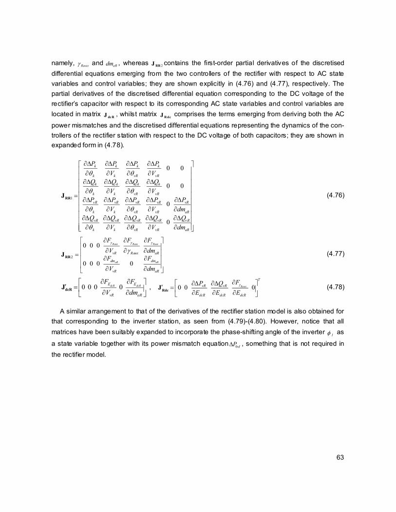
63
namely, Raux and aRdm , whereas 2RRJ contains the first-order partial derivatives of the discretised
differential equations emerging from the two controllers of the rectifier with respect to AC state
variables and control variables; they are shown explicitly in (4.76) and (4.77), respectively. The
partial derivatives of the discretised differential equation corresponding to the DC voltage of the
rectifier’s capacitor with respect to its corresponding AC state variables and control variables are
located in matrix dcRJ , whilst matrix
RdcJ comprises the terms emerging from deriving both the AC
power mismatches and the discretised differential equations representing the dynamics of the con-
trollers of the rectifier station with respect to the DC voltage of both capacitors; they are shown in
expanded form in (4.78).
1
0 0
0 0
0
0
k k k k
k k vR vR
k k k k
k k vR vR
vR vR vR vR vR
k k vR vR aR
vR vR vR vR vR
k k vR vR aR
P P P P
V V
Q Q Q Q
V V
P P P P P
V V dm
Q Q Q Q Q
V V dm
RRJ (4.76)
2
0 0 0
0 0 0 0
Raux Raux Raux
aR aR
vR Raux aR
dm dm
vR aR
F F F
V dmF F
V dm
RRJ (4.77)
0 0 0 0dcR dcRE E
vR aR
F F
V dm
dcRJ , 0 0 0Raux
T
vR vR
dcR dcR dcR
FP Q
E E E
RdcJ (4.78)
A similar arrangement to that of the derivatives of the rectifier station model is also obtained for
that corresponding to the inverter station, as seen from (4.79)-(4.80). However, notice that all
matrices have been suitably expanded to incorporate the phase-shifting angle of the inverter I as
a state variable together with its power mismatch equation0vIP , something that is not required in
the rectifier model.

64
1
0 0
0 0 0
0 0 0
0
0
0 0
m m m m
m k vI vI
m m m m
m k vI vI
vI vI vI vI vI vI
m k vI vI I aI
vI vI vI vI vI vI
m k vI vI I aI
vI vI
vI vI
P P P P
V V
Q Q Q Q
V V
P P P P P P
V V dm
Q Q Q Q Q Q
V V dm
P P
V
IIJ
0 00vI vI
I aI
P P
dm
(4.79)
2
0 0 0 0 0 0
0 0 0 0 0
dcIaux
aI aI
I
dcIaux
dm dm
vI aI
F
IF F
V dm
IIJ , 00 0 0dcIaux
T
IvI vI vI
dcI dcI dcI dcI
FP Q P
E E E E
IdcJ (4.80)
Completion of the VSC-HVDC model for positive-sequence, time domain simulations requires
encompassing all the derivative terms corresponding to the DC circuit of the VSC-based transmis-
sion system; the linearisation of the equations arising from the DC voltage and current dynamics of
the capacitors and inductors, respectively, together with those pertaining to the power mismatches
at both ends of the DC cable are shown in (4.81).
0 0 0
0 0 0
0 0 0 0
0 0 0 0
0 0 0
0 0 0
Rx Rx Rx
Ix Ix Ix
dcR dcR
dcI dcI
I I I
Rx dcR dcRx
I I I
Ix dcI dcIx
E E
Rx dcR
E E
Ix dcI
Rx Rx Rx
Rx dcRx dcIx
Ix Ix Ix
Ix dcRx dcIx
F F F
I E EF F F
I E EF F
I EF F
I EP P P
I E EP P P
I E E
dcJ
(4.81)
It is worth emphasising that the sparse nature of the overall linearised VSC-HVDC link model for
dynamic simulations, as in the case of the steady-state model, is favourable in actual software
implementations if sparsity techniques are used. The mismatch powers and their corresponding
state and control variables are shown in (4.75) and (4.82)-(4.83), respectively. It is envisaged that
the encompassing manner in which the dynamic HVDC model has been developed may give rise
to a generalisation of multi-terminal arrangements of conveters for VSC-upgraded power networks.

65
0
Raux aR
dcIaux aI
Rx Ix dcR dcI
T
k k vR vR dm
T
m m vI vI vI I dm
T
I I E E Rx Ix
P Q P Q F F
P Q P Q P F F
F F F F P P
R
I
dc
F
F
F
(4.82)
T
k k vR vR Raux a R
T
m m vI vI I dcIaux aI
T
Rx Ix dcR dcI dcRx dcIx
V V dm
V V I dm
I I E E E E
R
I
dc
ΔΦ
ΔΦ
ΔΦ
(4.83)
4.2.2 VSC-HVDC dynamic model with frequency regulation capabilities
VSC-HVDC systems are designed to serve in a wide range of power systems applications such as
interconnecting AC networks of the same or different frequencies, supplying electrical energy to
remote islands and off-shore oil and gas platforms, in-feeding of high load points in city centres
and the exporting of the electrical energy from off-shore wind parks. In certain applications, it is
desirable to exert some influence upon those relatively small networks, often referred to as low-
inertia networks or AC microgrids, through the DC link with the aim of making their operation more
stable. Perhaps, power fluctuations is the most severe problem these networks face; they lack
inertial and primary frequency response due to the non-existance of power controlling devices
such as battery energy storage systems or synchronous generators with speed-governing systems.
In fact, these island systems may be built without any type of power generating units, e.g. a
passive network consisting of only passive loads. In near-zero inertia electrical networks, even a
very small power imbalance would lead the frequency to experience large rises or drops,
depending on the nature of the power imbalance. This situation would arise when power
imbalances occur in an AC power network with little or no inertia and fed by a VSC-HVDC link
because VSC converters do not possess the ability to strengthen, on their own, the inertial
response or to aid the primary frequency control of AC networks. In this context, aiming at
investigating the feasibility of counting on frequency support in near-zero inertia electrical networks,
a VSC-HVDC dynamic model with frequency regulation capabilities is developed. The model ought
to be applicable to HVDC links feeding into independent, low-inertia networks.
A frequency deviation in a network arises from a mismatch between the mechanical power and
the electrical power in a synchronous machine. These frequency deviations are larger in the
smaller synchronous generators owing to their lighter rotating masses. As a matter of fact, the
inertia constant of the generator is the parameter that determines the size of the frequency
deviation following a power imbalance event. Besides the inertial response exhibited by
synchronous generators, most of them are fitted with speed-governing controls to bring about a

66
degree of power controllability into the generating system, which is said to exert primary-frequency
control. At least from the conceptual point of view, a parallel may be drawn between the kinetic
energy stored in the rotating mass of a synchronous generator relating to its inertia constant and
the electrostatic and electromagnetic energies stored in the capacitors and inductors placed at the
DC side of the VSC-based transmission system, respectively, which will also have an inertia
constant c iH H H , albeit of a much smaller dimension than the inertia constant of a
synchronous machine. Furthermore, the difference between the DC power entering the inverter
dcI dcIE I and the power 0 v IP will give rise to a frequency deviation in the network connected to the
inverter. Hence, the angular speed I and the angle I of the inverter station are dynamically
computed as shown in (7.84)-(7.85) (Castro and Acha, 2015b).
0I
dcI dcI vI
dK E I P
dt
(7.84)
2II Inom
df
dt
(7.85)
where InomK f H and
Inomf [Hz] represents the nominal electrical frequency of the island network.
Its value may be the same or different from that of the main utility grid connected at the rectifier AC
terminal. It should be remarked that the angle I as well as the angular speed I become the
reference signals for the near-zero inertia network.
Given that the total fictitious inertia of the inverter H is very small (let us say 10 ms), in the
event of relatively small power disturbances, big sags or swells in the angular speed would be
caused. To prove this point, let us take the case of a low-inertia grid operating at 60 Hz, where the
value of K would be around 18.85x10³; if the power imbalance is in the order of P -1x10⁻³ p.u.
and there is no power control action after only one second, t 1 s, then the speed deviation
would be: K P t -18.85 rad/s, which in terms of frequency is If 57 Hz. This would be a
critical problem that should not be overlooked when the island network contains frequency-
sensitive loads. In these cases, there is a need for implementing a practical solution to mitigate the
frequency excursions. An alternative is to import electrical power from the main utility grid through
the HVDC link. Hence, in these conditions, the VSC-HVDC model ought to depart from the idea of
transmitting a fixed amount of power between two interconnected networks which, so far, has been
the main functionality sought from HVDC applications. To this end, the auxiliary control loop shown
in Figure 4.9 is designed to enable the VSC-HVDC link to import the power required from the
system connected at the rectifier AC terminal to satisfy any power mismatch taking place in the AC
island network, with the inverter station acting as a power electronic source with active and
reactive power control capabilities. The control loop measures the actual angular speed of the
island network, which happens to be the same as I , and compares it with its nominal one,

67
2In om In omf . The error is processed by a PI controller to adjust the angular aperture between
the AC system voltage phase angle vR and the phase-shifting angle of the rectifier
R (Castro and
Acha, 2015b).
Figure 4.9 Frequency controller of the VSC-HVDC link
It should be remarked that while the aim of the controller shown in Figure 4.7 is to attain a fixed
power transfer in the DC link, the target of the VSC-HVDC controller shown in Figure 4.9 is to
maintain the electrical frequency of the network connected to the inverter within safe limits by
modifying the extracted power from the grid connected to the rectifier AC terminal. This means that
the value of the DC power transfer will be one, for instance, that brings the frequency of the island
grid back to its nominal steady-state value. The equations that enable the calculation of the
dynamic behaviour of the DC power when the inverter station of the HVDC system is acting as a
power electronic source with frequency regulation capabilities are expressed as (7.86)-(7.87).
Rauxi Inom I
dK
dt
(7.86)
R p Inom I RauxK (7.87)
As in the case of the VSC-HVDC model aimed at scheduled DC power regulation presented in
Section 4.2.1, the set of power flow equations for the two interconnected AC networks together
with the differential-algebraic equations pertaining to the synchronous generators and their
controllers, induction machines, etc., as well as the HVDC’s algebraic and discretised differential
equations, are solved simultaneously using the trapezoidal method and the Newton’s algorithm.
For the sake of completeness, the overall mismatch expressions that must be solved together with
the equations of the whole network, at every integration step t , are shown in (4.88)-(4.107)
(Castro and Acha, 2015b).
calk kltc dk kP P P P (4.88)
calk kltc dk kQ Q Q Q (4.89)
vR vR dvR vRltcP P P P (4.90)

68
vR vR dvR vRltcQ Q Q Q (4.91)
calm mltc dm mP P P P (4.92)
calm mltc dm mQ Q Q Q (4.93)
vI vI dvI vIltcP P P P (4.94)
vI vI dvI vIltcQ Q Q Q (4.95)
Rx dcRx Rx dcRP E I P (4.96)
Ix dcIx Ix dcIP E I P (4.97)
( ) ( ) ( ) ( )0.5 0.5dcRE dcR t t dcR t t dcR t dcR tF E tE E tE (4.98)
( ) ( ) ( ) ( )0.5 0.5dcIE dcI t t dcI t t dcI t dcI tF E tE E tE (4.99)
( ) ( ) ( ) ( )0.5 0.5RxI Rx t t Rx t t Rx t Rx tF I t I I t I (4.100)
( ) ( ) ( ) ( )0.5 0.5IxI Ix t t Ix t t Ix t Ix tF I t I I t I (4.101)
( ) ( ) ( ) ( )0.5 0.5dcIauxI dcIaux t t dcIaux t t dcIaux t dcIaux tF I t I I t I (4.102)
( ) ( ) ( ) ( )0.5 0.5Raux Raux t t Raux t t Raux t Raux tF t t (4.103)
( ) ( ) ( ) ( )0.5 0.5aRdm aR t t aR t t aR t aR tF dm tdm dm tdm (4.104)
( ) ( ) ( ) ( )0.5 0.5aIdm aI t t aI t t aI t aI tF dm tdm dm tdm (4.105)
( ) ( ) ( ) ( )0.5 0.5I I t t I t t I t I tF t t (4.106)
( ) ( ) ( ) ( )0.5 0.5I I t t I t t I t I tF t t (4.107)
Notice the reformulation that has taken place in the above set of equations in comparison with
the previously developed VSC-HVDC dynamic model, shown in Section 4.2.1. This is to endow the
HVDC link with frequency regulation capabilities. Now the model incorporates two differential
equations (4.106)-(4.107) that enable the computation of the reference angle and angular speed of
the independent AC network connected at the inverter AC terminal. Furthermore, contrary to the
customary objective of the power angle controller of the VSC-HVDC link, equation (4.103)
represents the DC power controller that acts upon changes in the frequency of the grid connected
at the inverter AC terminal. The above set of equations yields the linearised structure given in
(4.108) for the VSC-HVDC model with frequency regulation capabilities. Advantageously, this is
very similar to that derived for the VSC-HVDC model with power regulation capabilities
represented by (4.75). However, it stands out from (4.108) that a full decoupling between the

69
rectifier and inverter no longer exists. In this particular case, the utilisation of the angular speed
measurement by the frequency controller of the rectifier produces a mutual matrix term between
both converters; this is matrix R IJ given in (4.109) which accommodates the derivative of the
discretised differential equation of the frequency controller with respect to the actual angular speed
of the island network I .
1
2
1
2
i
i i
RRRdc
RR RI
R RII
I Idc III
dc dc
dcR dc
J 0J
J JF ΔΦ
JF 0 J ΔΦ
JF ΔΦ
J 0 J
(4.108)
0 0 0 0 0 0 0
0 0 0 0 0 0 0 0
Raux
I
F
RIJ (4.109)
Some modifications in matrices 2RRJ ,
RdcJ , 1IIJ ,
2I IJ and I dcJ take place to be consistent with
this control strategy. The new Jacobian entries are shown in equations (4.110)-(4.113).
2
0 0 0 0 0
0 0 0 0
Raux
aR aR
Raux
dm dm
vR aR
F
F F
V dm
RRJ , 0 0 0 0
T
vR vR
dcR dcR
P Q
E E
RdcJ (4.110)
1
0 0 0 0
0 0 0 0
0 0
0 0
m m m m
m m vI vI
m m m m
m m vI vI
vI vI vI vI vI vI
m m vI vI aI I
vI vI vI vI vI vI
m m vI vI aI I
P P P P
V V
Q Q Q Q
V V
P P P P P P
V V dm
Q Q Q Q Q Q
V V dm
IIJ
(4.111)

70
2
0 0 0 0 0 0 0
0 0 0 0 0 0
0 0 0
0 0 0 0 0 0
dcIaux
aI aI
I I I I I
I I
I
dcIaux
dm dm
vI aI
vI vI aI I I
I I
F
IF F
V dmF F F F F
V dmF F
IIJ (4.112)
0 0 0 0dcIaux I
T
IvI vI
dcI dcI dcI dcI
F FP Q
E E E E
IdcJ (4.113)
The modified vectors of mismatches and increments of the VSC-HVDC link model with
frequency regulation are shown in (4.114).
dcIaux aI I I
T
m m vI vI I dm
T
m m vI vI dcIaux aI I I
P Q P Q F F F F
V V I dm
I
I
F
ΔΦ
(4.114)
4.3 Multi-terminal VSC-HVDC systems for dynamic simulations
Worldwide point-to-point HVDC systems have been so far realised to provide access to remote
load points or to facilitate power exchange over very long distances between, for instance, two
otherwise independent systems. Due to the fact that only two partners interact in point-to-point
VSC-HVDC connections, this hinders the possibility of connecting an additional AC system which
may lie within the reach of the DC transmission routing. This limitation has urged companies to
make sudden advances in the direction of multi-terminal direct current transmission schemes,
multi-terminal VSC-HVDC systems able to adapt easily to the always varying conditions of power
networks, facilitating simultaneously the control of the power flowing into or from the DC high
power transmission system. Clearly the operation of multi-terminal HVDC systems is more
challenging and complex in comparison with former point-to-point connections of power converters;
hence, this breakthrough must come with corresponding advances in the arena of modelling and
simulation of multi-terminal HVDC systems to aid power system engineers to confront the soon-to-
emerge challenges relating to their planning, operation and control.
In a multi-terminal arrangement, balancing the currents of the different converter stations
comprising the VSC-based multi-terminal network is one of the main pursued objectives to ensure

71
a reliable operation not only for the HVDC system itself, but also for the various interconnected
networks. Power reallocation and control of the voltage profile on the meshed DC network are also
primary functions that must be pursued in a multi-terminal scheme. The control system of each
VSC station has to provide a rapid response to recover safely after faults occurring either in the AC
system or in the DC system. At least from the conceptual standpoint, it is expected that all benefits
gained with the use of two-terminal HVDC systems be inherited to multi-terminal schemes. Also, it
is very likely, if not a fact, that the same advantages attained in meshed AC networks, where the
power supply to users even during abnormal conditions is ensured, will be also gained in multi-
terminal HVDC systems.
At the planning stage of power systems, to carry out holistic assessments of multi-terminal
VSC-HVDC systems together with the interconnected AC networks requires suitable VSC models.
System-wide dynamic studies of practical networks would benefit from a modular approach, one
that enables efficient simulations without jeopardising the accuracy of the results, and at the same
time, one that does not exclude the computation of essential state and control variables pertaining
to the converter stations. Throughout Chapter 3, particularly in Section 3.5, it was shown that the
fundamental VSC station model possesses a high degree of modelling flexibility allowing a
straightforward aggregation of a number of VSC stations to give rise to any type of multi-terminal
arrangement. The same modular modelling approach is followed for the dynamic regime, one
where each VSC unit of the multi-terminal HVDC dynamic model is seen to consist of a power
converter, phase reactor, filter capacitor and an interfacing OLTC transformer to connect to the
high-voltage AC network, being in the opposite side of the VSC, the DC bus which connects to an
arbitrary DC grid, as shown in Figure 4.10 (Castro and Acha, 2016).
Figure 4.10 Full VSC station with ancillary elements
4.3.1 Three-terminal VSC-HVDC dynamic model
Three types of converters were defined, for the steady-state operating regime, to conform with
their specific control strategy and pairing AC network: the slack converter controlling its DC voltage
- VSCSlack , the converter controlling its DC power - VSCPsch and the converter feeding into a
passive network - VSCPass. By the same token, the modelling of each one of these converters is

72
also envisaged in the modelling of VSC-based multi-terminal connections for the dynamic
operating regime. To such an end, the basic three-terminal VSC-HVDC system, depicted in Figure
4.11, is initially formulated; this is a VSC-based transmission system that accomodates the afore-
mentioned three types of converters. This system is then expanded quite naturally to build up a
model that comprises a number of VSC units which is commensurate with the number of terminals
in the HVDC system, suitably accommodated in a unified frame-of-reference aimed at positive-
sequence dynamic simulations of power networks (Castro and Acha, 2016).
Figure 4.11 Representation of a three-terminal VSC-HVDC link and its control variables
The VSC-based transmission system shown in Figure 4.11 comprises three converters, where
for simplicity of representation, the associated phase reactor and AC filter capacitor of each
converter have been omitted. Converter 1 is of type VSCSlack whereas converters 2 and 3 are
assumed to be of type VSCPsch and VSCPass, respectively. Each VSC unit may be seen to consist
of a power converter, AC phase reactor, AC filter capacitor and an interfacing OLTC transformer to
connect to each particular AC network. For simplicity of representation, the associated AC phase
reactor and AC filter capacitor of each converter have been omitted in the figure, but their incorpo-
ration is quite a straightforward matter. On the opposite side of each VSC there is the DC bus
which, in this particular case, connects to a capacitor and smoothing inductor and resistor, forming
a delta connection with cables of resistance 4dcR ,
5d cR and 6dcR . Notice that in a multi-terminal
scheme, any converter can play the role of either a rectifier or inverter according to the actual con-
ditions of power exchange between the converters and the formed DC grid or according to the par-

73
ticular requirements of the network connected at their corresponding AC terminal. Therefore, for
simplicity of developments, the subscripts R and I formerly standing for rectifier and inverter,
respectively, have been changed by suitable numbers.
In connection with Figure 4.11, the voltage and current of the capacitors and inductors,
respectively, are computed as shown in (4.115)-(4.116).
1 1 1
1
dc dc x
d c
dE I I
dt C
, 2 2 2
2
dc dc x
dc
dE I I
dt C
, 3 3 3
3
dc dc x
dc
dE I I
dt C
(4.115)
1 1 4
1
x dc dc
dc
dI E E
dt L
, 2 2 5
2
x dc dc
dc
dI E E
dt L
, 3 3 6
3
x dc dc
dc
dI E E
dt L
(4.116)
In this particular case, the VSC station 1 is charged with the DC voltage control of the three-
terminal VSC-based system. This implies that this VSC plays the role of the slack converter for the
DC network. Figure 4.12 shows the DC voltage controller for the slack converter VSCSlack whose PI
controller is used to process the error between the actual voltage of the converter’s DC bus and its
nominal one, 1d cE and
dcnomE , respectively, obtaining new values of its DC current 1dcI (Castro and
Acha, 2016).
Figure 4.12 DC voltage dynamic controller of the slack converter VSCSlack
Simultaneously, the other two VSC stations are responsible for controlling the power at its
corresponding DC bus, but the power control objectives are different from each other. The aim of
the converter of type VSCPsch is to achieve a fixed, scheduled DC power transfer. On the contrary,
the converter of type VSCPass, whose main goal is to provide frequency support to the network
connected at its AC terminal, regulates the power injection into the passive network as a function
of the power deviations in such AC grid. Figure 4.13 shows the control loops for these two
converter stations. Notice that the converter of type VSCPsch pursues a power balance at its DC
bus by regulating the angular aperture between its phase-shifting angle and its corresponding AC
voltage angle whilst the converter of type VSCPass acts upon variations on the frequency measured
at its AC terminal, increasing or decreasing its DC current depending on the actual conditions
(Castro and Acha, 2016).

74
Figure 4.13 (a) DC-power controller of the converter of type VSCPsch and (b) Frequency controller of the converter of type VSCPass
As it is standard practice in two-terminal HVDC systems, the modulation index of each VSC
station is responsible for controlling the voltage magnitude at the corresponding AC terminal. In
this particular case, the VSC stations bring about three control loops aimed at controlling the
voltage magnitude at each AC terminal of the three-terminal VSC-based transmission system.
Each control loop comprises a first-order control block whose aim is also to readjust each
corresponding modulation index according to the difference between the scheduled voltage
magnitudes and the actual voltage at the nodes where the converters are connected, as shown in
Figure 4.14. Notice that each control loop acts autonomously, needing no feedback inputs coming
from the rest of the modulation index controllers; this implies that no communication is needed
between the converters comprised in the multi-terminal system as far as AC voltage control is
concerned.
Figure 4.14 Modulation index controllers of the three converter stations making up the three-terminal HVDC system
Clearly, this three terminal HVDC system has increased in terms of complexity, bringing about
nine DC buses. Unlike point-to-point HVDC connections where the resistor value corresponding to
the DC smoothing inductor can be simply added to the DC cable resistor, in a multi-terminal con-
nection, as the one being addressed in this case, the resistor of each DC smoothing inductor pro-
duces an additional node in the DC system. However, its inclusion in the proposed formulation can

75
be carried out straightforwardly. The calculated power injections at each node of the DC system
are computed as shown in (4.117). For practical reasons, this expression only includes the compu-
tation of the power injections at the DC buses of the purely resistive network, which is formed from
bus 4 to bus 9. Evidently, during steady conditions, the voltage at the DC bus of the three
converters equals the voltage at buses 4, 5 and 6, respectively.
92
4
caldcj dcj dcjj dcj dcm dcjm
jm j
P E G E E G
(4.117)
Admittedly, the most basic multi-terminal HVDC arrangement, shown in Figure 4.11, encom-
passes the most representative AC/DC components that may have a significant impact on its dy-
namics. Nevertheless, if efficient, reliable solutions are pursued for dynamic simulations, the use of
a generalised approach, one very similar to that employed in point-to-point HVDC configurations, is
essential to carry out simulations of multi-terminal HVDC systems.
The differential equations, shown in (4.118)-(4.131), arise from the voltage and current
dynamics of the capacitors and inductors as well as from the controllers of the three-terminal VSC-
HVDC link model (Castro and Acha, 2016).
1 1( ) 1( ) 1( ) 1( )0.5 0.5
dcE dc t t dc t t dc t dc tF E tE E tE (4.118)
2 2( ) 2( ) 2( ) 2( )0.5 0.5
dcE dc t t dc t t dc t dc tF E tE E tE (4.119)
3 3( ) 3( ) 3( ) 3( )0.5 0.5
dcE dc t t dc t t dc t dc tF E tE E tE (4.120)
1 1 ( ) 1 ( ) 1 ( ) 1 ( )0.5 0.5
xI x t t x t t x t x tF I t I I t I (4.121)
2 2 ( ) 2 ( ) 2 ( ) 2 ( )0.5 0.5
xI x t t x t t x t x tF I t I I t I (4.122)
3 3 ( ) 3 ( ) 3 ( ) 3 ( )0.5 0.5
xI x t t x t t x t x tF I t I I t I (4.123)
1 1 ( ) 1 ( ) 1 ( ) 1 ( )0.5 0.5
dc auxI dc aux t t dc aux t t dc aux t dc aux tF I t I I t I (4.124)
2 2 ( ) 2 ( ) 2 ( ) 2 ( )0.5 0.5
aux aux t t aux t t aux t aux tF t t (4.125)
3 3 ( ) 3 ( ) 3 ( ) 3 ( )0.5 0.5
dc auxI dc aux t t dc aux t t dc aux t dc aux tF I tI I tI (4.126)
3 3( ) 3( ) 3( ) 3( )0.5 0.5t t t t t tF t t (4.127)
3 3( ) 3( ) 3( ) 3( )0.5 0.5t t t t t tF t t (4.128)
1 1( ) 1( ) 1( ) 1( )0.5 0.5
adm a t t a t t a t a tF dm tdm dm tdm (4.129)
2 2( ) 2( ) 2( ) 2( )0.5 0.5
adm a t t a t t a t a tF dm tdm dm tdm (4.130)

76
3 3( ) 3( ) 3( ) 3( )0.5 0.5
adm a t t a t t a t a tF dm tdm dm tdm (4.131)
The above set of expressions determine the whole dynamics in the three-terminal HVDC
system, however, the adopted formulation, which is based on power injections, requires additional
AC and DC power balance equations to complete the positive-sequence dynamic model.
The active and reactive power mismatch equations at the AC terminal of each VSC unit are
given by (4.132)-(4.143). Notice that, for the sake of completeness, these equations include the
power mismatch expressions corresponding to both ends of each converter’s OLTC transformer.
calk kltc dk kP P P P (4.132)
calk kltc dk kQ Q Q Q (4.133)
1 1 1 1v v dv v ltcP P P P (4.134)
1 1 1 1v v dv v ltcQ Q Q Q (4.135)
calm mltc dm mP P P P (4.136)
calm mltc dm mQ Q Q Q (4.137)
2 2 2 2vI v dv v ltcP P P P (4.138)
2 2 2 2v v dv v ltcQ Q Q Q (4.139)
caln nltc dn nP P P P (4.140)
caln nltc dn nQ Q Q Q (4.141)
3 3 3 3v v dv v ltcP P P P (4.142)
3 3 3 3v v dv v ltcQ Q Q Q (4.143)
In connection with Figure 4.11, the purely resistive network, formed by nodes 7, 8 and 9,
produces the mismatch equations (4.147)-(4.149). Furthermore, the coupling between this resistive
network and the DC side of the power converters is given at the DC nodes 4, 5, and 6; the power
mismatch expressions at these nodes are shown in (4.144)-(4.146).
4 4 1 4cal
dc dc x dcP E I P (4.144)
5 5 2 5cal
dc dc x dcP E I P (4.145)
6 6 3 6cal
dc dc x dcP E I P (4.146)

77
7 7 7cal
dc d dcP P P (4.147)
8 8 8cal
dc d dcP P P (4.148)
9 9 9cal
dc d dcP P P (4.149)
where the powers 7dP , 8dP and 9dP stand for the powers drawn by DC loads at the nodes that
make up the delta arrangement of DC cables, but in this particular scenario they take the value of
zero; the power expressions 4cal
dcP to 9cal
dcP represent the calculated powers at the corresponding
nodes whose calculation is carried out using (4.117). In addition to the above mismatch expres-
sions, the equation shown in (4.150) enables the computation of the power exchange between the
AC and DC sides of the slack converters VSCSlack .
1 1 1 0 1dc dc dc vP E I P (4.150)
This last algebraic equation implies that the internal power equilibrium of the slack converter is
attained instantaneously, something that does not occur in converters of type VSCPsch and VSCPass.
In these two converters, whose aim is to provide power regulation and frequency support, the
internal power equilibrium is reached with a time delay; a time that is imposed by the speed
response involved in their corresponding dynamic controllers depicted in Fig. 4.13. Such time
delay will cause a momentary energy mismatch, charging or discharging the existing capacitors
and inductors of the DC grid. Therefore it can be inferred that the response time of these two
controllers will directly impact the magnitude of the DC voltage deviations when the AC/DC system
is subjected to disturbances.
The overall three-terminal HVDC model for positive-sequence dynamic simulations is defined by
equations (4.118)-(4.150). The linearised form of this model is given by (4.151); the unified frame
of reference pursued in this formulation suitably combines the whole set of differential and
algebraic equations arising from the AC/DC system formed by the three VSC stations (Castro and
Acha, 2016).
i i i
Slack Slack Sdc Slack
Psch Psch Psdc Psch
Pass Pass Padc Pass
dc dcS dc dc
F J 0 0 J ΔΦ
F 0 J 0 J ΔΦ
F 0 0 J J ΔΦ
F J 0 0 J ΔΦ
(4.151)
were the 0 entries are zero-padded matrices of suitable orders and all matrix entries are addition-
ally divided for simplicity of presentation and analysis, as shown in (4.152)-(4.153).

78
SlackSlack
Slack
JJ
J,
PschPsch
Psch
JJ
J,
PassPass
Pass
JJ
J (4.152)
Sdc SdcJ 0 J 0 , Psdc PsdcJ 0 J 0 , Padc P adcJ 0 J 0 , T
dcS dcSJ 0 J 0 (4.153)
Matrices Sla ckJ ,
PschJ and PassJ accommodate the derivative terms of the AC power mismatches
of the three types of converters with respect to their corresponding AC state variables and control
variables, as shown in (4.154)-(4.156). Notice that PassJ also makes provision for the derivatives
with respect to the electrical reference variables of the passive network, 3 and
3 .
1 1
1 1
1 1 1 1 1 1
1 1 1 1
1 1 1 1 1 1
1 1 1 1
1 1
1
0 0 0
0 0 0
0
0
0 0
k k k k
k k v v
k k k k
k k v v
v v v v v v
k k v v a
v v v v v v
k k v v a
dc dc
v
P P P P
V V
Q Q Q Q
V V
P P P P P P
V V dm
Q Q Q Q Q Q
V V dm
P P
V
SlackJ
1 1
1 1 1
0dc dc
v a
P P
dm
(4.154)
2 2
2 2
2 2 2 2 2
2 2 2
2 2 2 2
2 2 2
0 0
0 0
0
0
m m m m
m m v v
m m m m
m m v v
v v v v v
m m v v a
v v vR v v
m m v v a
P P P P
V V
Q Q Q Q
V V
P P P P P
V V dm
Q Q Q Q Q
V V dm
PschJ (4.155)
3 3
3 3
3 3 3 3 3 3
3 3 3 3
3 3 3 3 3 3
3 3 3 3
0 0 0 0
0 0 0 0
0 0
0 0
n n n n
n n v v
n n n n
n n v v
v v v v v v
n n v v a
v v v v v v
n n v v a
P P P P
V V
Q Q Q Q
V V
P P P P P P
V V dm
Q Q Q Q Q Q
V V dm
PassJ
(4.156)
The derivative terms of the discretised differential equations arising from the dynamic controllers
of the VSC stations making up the three-terminal HVDC system with respect to their corresponding
AC state variables and control variables are suitably accommodated in matrices Sla ckJ ,
PschJ and
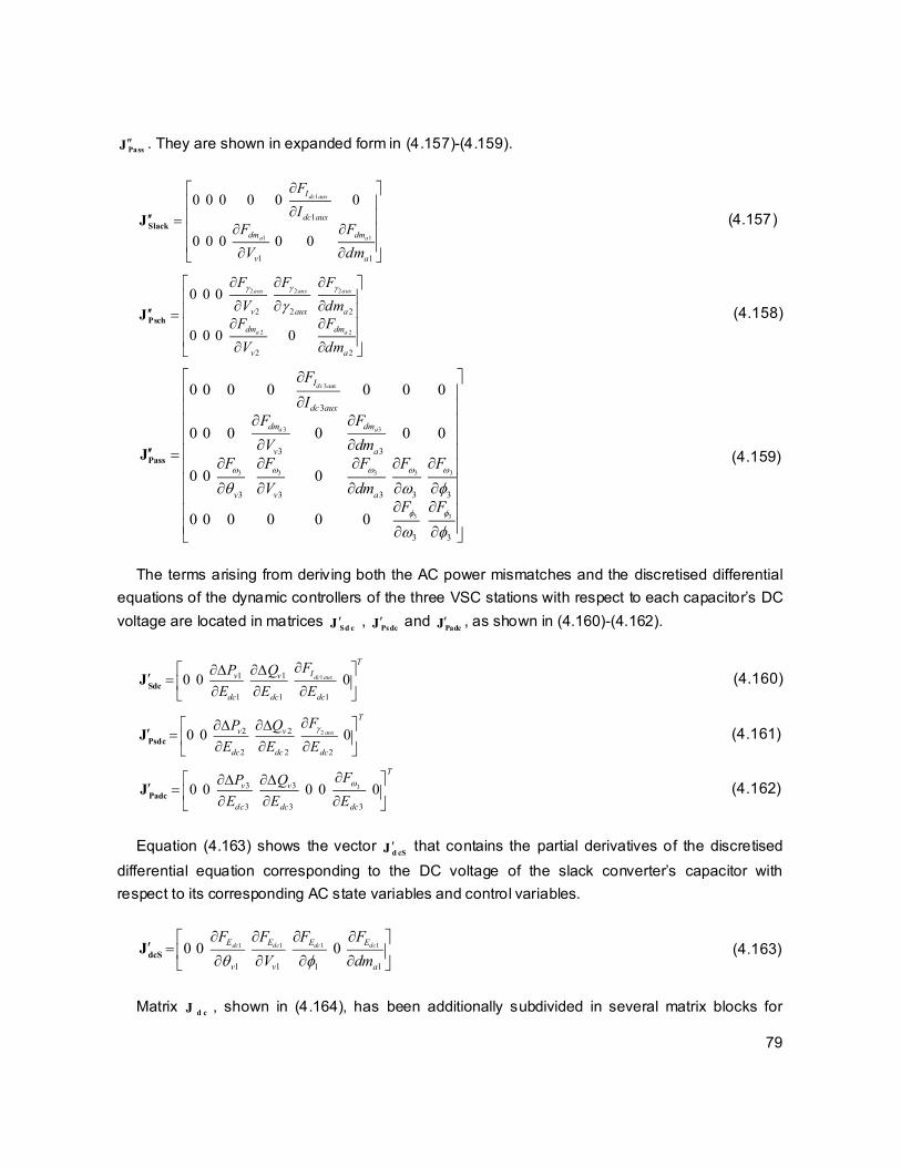
79
PassJ . They are shown in expanded form in (4.157)-(4.159).
1
1 1
1
1 1
0 0 0 0 0 0
0 0 0 0 0
dc aux
a a
I
dc aux
dm dm
v a
F
IF F
V dm
SlackJ (4.157)
2 2 2
2 2
2 2 2
2 2
0 0 0
0 0 0 0
aux aux aux
a a
v aux a
dm dm
v a
F F F
V dmF F
V dm
PschJ (4.158)
3
3 3
3 3 3 3 3
3 3
3
3 3
3 3 3 3 3
3 3
0 0 0 0 0 0 0
0 0 0 0 0 0
0 0 0
0 0 0 0 0 0
dc aux
a a
I
dc aux
dm dm
v a
v v a
F
IF F
V dmF F F F F
V dmF F
PassJ (4.159)
The terms arising from deriving both the AC power mismatches and the discretised differential
equations of the dynamic controllers of the three VSC stations with respect to each capacitor’s DC
voltage are located in matrices Sd cJ ,
PsdcJ and
PadcJ , as shown in (4.160)-(4.162).
11 1
1 1 1
0 0 0dc aux
T
Iv v
dc dc dc
FP Q
E E E
SdcJ (4.160)
22 2
2 2 2
0 0 0aux
T
v v
dc dc dc
FP Q
E E E
PsdcJ (4.161)
33 3
3 3 3
0 0 0 0 0
T
v v
dc dc dc
FP Q
E E E
PadcJ (4.162)
Equation (4.163) shows the vector d cSJ that contains the partial derivatives of the discretised
differential equation corresponding to the DC voltage of the slack converter’s capacitor with
respect to its corresponding AC state variables and control variables.
1 1 1 1
1 1 1 1
0 0 0dc dc dc dcE E E E
v v a
F F F F
V dm
dcSJ (4.163)
Matrix d cJ , shown in (4.164), has been additionally subdivided in several matrix blocks for

80
simplicity of future developments with a view to multi-terminal schemes. This matrix provides the
coupling between the DC cuircuit made up by the delta connection of DC cables and the three
VSC stations. This coupling emerges from suitably accommodating the derivatives of the
discretised differential equations of inductors current and capacitors voltage together with the
nodal power mismatches of the internal DC nodes, 4 to 9, with respect to suitable DC state and
control variables, i.e., the set of DC voltages and currents taking part in the dynamics of this three-
terminal HVDC system.
1 2 5
3 4
6 7
dc dc dc
dc dc dc
dc dc
J J J
J J J 0
J 0 J
(4.164)
where 5 5d c d cJ J 0 and 6 6
Tdc dcJ J 0 . The entries of the Jacobian matrix arising from the DC cir-
cuit are given, in explicit form, in (4.165)-(4.167),
1
2
3
1
1
2
3
0 0
0 0
0 0
x
x
x
I
xI
xI
x
F
IF
IF
I
dcJ ,
1
2
3
1
2
2
3
0 0
0 0
0 0
x
x
x
I
dcI
dcI
dc
F
EF
EF
E
dcJ ,
1
2
3
1
3
2
3
0 0
0 0
0 0
dc
dc
dc
E
xE
xE
x
F
IF
IF
I
dcJ
(4.165)
1
2
3
1
4
2
3
0 0
0 0
0 0
dc
dc
dc
E
dcE
dcE
dc
F
EF
EF
E
dcJ ,
1
2
3
4
5
5
6
0 0
0 0
0 0
x
x
x
I
dcI
dcI
dc
F
EF
EF
E
dcJ ,
4
15
6
26
3
0 0
0 0
0 0
dc
xdc
xdc
x
P
IP
IP
I
dcJ
(4.166)
4 4
4 7
5 5
5 8
6 6
6 97
7 7 7 7
4 7 8 9
8 8 8 8
5 7 8 9
9 9
6 7
0 0 0 0
0 0 0 0
0 0 0 0
0 0
0 0
0 0
dc dc
dc dc
dc dc
dc dc
dc dc
dc dc
dc dc dc dc
dc dc dc dc
dc dc dc dc
dc dc dc dc
dc dc
dc dc
P P
E EP P
E EP P
E EP P P P
E E E EP P P P
E E E EP P
E E
dcJ
9 9
8 9
dc dc
dc dc
P P
E E
. (4.167)

81
Clearly, the diagonal matrices shown in (4.165)-(4.166), whose order corresponds to the num-
ber of VSC stations, could be straightforwardly expanded to conform to any kind of multi-terminal
arrangement of converters.
The mismatch vectors and increments of the state and control variables for the three VSC units
and the DC circuit are shown in (4.168)-(4.169).
1 1
2 2
3 3 3 3
1 2 3 1 2 3
1 1 1
2 2
3 3
4 5 6 7 8 9
dc aux a
aux a
dc aux a
x x x dc dc dc
T
k k v v dc I dm
T
m m v v dm
T
n n v v I dm
T
I I I E E E dc dc dc dc dc dc
P Q P Q P F F
P Q P Q F F
P Q P Q F F F F
F F F F F F P P P P P P
Slack
Psch
Pass
dc
F
F
F
F
(4.168)
1 1 1 1 1
2 2 2 2
3 3 3 3 3 3
1 2 3 1 2 3 4 5 6 7 8 9
T
k k v v dc aux a
T
m m v v aux a
T
n n v v dc aux a
T
x x x dc dc dc dc dc dc dc dc dc
V V I dm
V V dm
V V I dm
I I I E E E E E E E E E
Slack
Psch
Pass
dc
ΔΦ
ΔΦ
ΔΦ
ΔΦ
(4.169)
Notice that the vector d cΔΦ not only contains DC voltages as state variables, as it is the case
for the three-terminal HVDC steady-state model derived in Section 3.5.1, but also it includes the
DC currents of the inductors. The increments of the state variables of both the converters and DC
circuit, calculated at iteration i, are used to update the state variables, using (4.170).
1
1
1
1
i i i
i i i
i i i
i i i
Slack Slack Slack
Psch Psch Psch
Pass Pass Pass
dc dc dc
Φ Φ ΔΦ
Φ Φ ΔΦ
Φ Φ ΔΦ
Φ Φ ΔΦ
(4.170)
4.3.2 Multi-terminal VSC-HVDC dynamic model
The three-terminal HVDC dynamic model synthesised by equation (4.151) demonstrates that the
three types of VSCs can be straightforwardly combined in a unified frame of reference. Expanding
further such representation, a multi-terminal arrangement of VSCs possessing an arbitrary DC
network topology and a number of converter stations can be tailored, as shown in the general ex-
pression given by (4.171). Moving towards multi-terminal schemes, expression (4.151) requires

82
being properly expanded to make provisions for m converter stations of type VSCSlack, n converter
stations of type VSCPsch and r converter stations of type VSCPass (Castro and Acha, 2016).
1 1
1 1
1 1
i i
m m
n n
r r
Slack Slack Sl
Sdc
Slack Slack
Psch Psch
Psdc
Psch Psch
Pass Pass
Padc
Pass Pass
dc dcS dc
F J 0 ΔΦ0 0 J
F 0 JF J 0
0 0 JF 0 JF J 0
0 0 JF 0 J
F J 0 0 J
1
1
1
i
m
n
r
ack
Slack
Psch
Psch
Pass
Pass
dc
ΔΦΔΦ
ΔΦΔΦ
ΔΦ
ΔΦ
(4.171)
As implied from this last equation, there will be a number of zero-padded matrices and vectors
0. In expression (4.171), the mismatch terms F and the vectors of state variables increments
ΔΦ take the form of (4.168)-(4.169) depending on the type of converter, i.e., VSCSlack , VSCPsch or
VSCPass. Likewise, matrices J with subscripts Slack , Psch and Pass take the form of (4.152).
Caution has to be exercised because the non-zero entries of vectors S dcJ ,
PsdcJ , PadcJ and
dcSJ ,
need to be suitably staggered, something that is well exemplified by the three-terminal case. Pre-
serving the same accommodation of the DC state variables as that of the three-terminal case, the
vectors and matrices, which have a location corresponding to any of the DC network variables,
d cΔΦ , have the structure shown in equations (4.172)-(4.175).
1
m
Sdc
Sdc
Sdc
J 00 0 0 0J
0 0 0 J 0 0
(4.172)
1
n
Psdc
Psdc
Psdc
J 00 0 0 0J
0 0 0 J 0 0
(4.173)
1
r
Padc
Padc
Padc
J 00 0 0 0J
0 0 0 J 0 0
(4.174)
1
T
m
dcS
dcS
dcS
J 00 0 0 0J
0 0 0 J 0 0
(4.175)
The various entries in (4.172)-(4.175) are vectors with the generic j th terms depending on the
number and type of converter, with 1,...,j m , 1,...,j n and 1,...,j r for converters VSCSlack, VSCP-
sch or VSCPass, respectively. They are shown in equations (4.176)-(4.179).

83
0 0 0dcjaux
T
Ivj vj
dcj dcj dcj
FP Q
E E E
SdcJ (4.176)
0 0 0jaux
T
vj vj
dcj dcj dcj
FP Q
E E E
PsdcJ (4.177)
0 0 0 0 0j
T
vj vj
dcj dcj dcj
FP Q
E E E
PadcJ (4.178)
0 0 0dcj dcj dcj dcjE E E E
vj vj j aj
F F F F
V dm
dcSJ (4.179)
The Jacobian matrix of the DC network takes the general form of equation (4.180).
1 2 5
3 4
6 7
dc dc dc
dc dc dc
dc dc
J J J
J J J 0
J 0 J
(4.180)
where 5 5dc dcJ J 0 and 6 6
Tdc dcJ J 0 . The matrices from
1d cJ to 4d cJ ,
5d cJ and
6d cJ are diagonal
matrices of order vscn m n r , which stands for the total amount of converters making up the mul-
ti-terminal system, with 1,..., vscj n and 1, ..., 2vsc vsck n n . Such matrices are presented in an ex-
plicit form as shown in equations (4.181)-(4.182).
1
0 0
0 0
0 0
jx
jx
I
jx
I
jx
F
I
F
I
dcJ , 2
0 0
0 0
0 0
jx
jx
I
dcj
I
dcj
F
E
F
E
dcJ , 3
0 0
0 0
0 0
dcj
dcj
E
jx
E
jx
F
I
F
I
dcJ (4.181)
4
0 0
0 0
0 0
dcj
dcj
E
dcj
E
dcj
F
E
F
E
dcJ , 5
0 0
0 0
0 0
jx
jx
I
dck
I
dck
F
E
F
E
dcJ , 6
0 0
0 0
0 0
dck
jx
dck
jx
P
I
P
I
dcJ (4.182)
On the other hand, the order of matrix 7d cJ , shown in (4.183), corresponds to the number of
DC nodes dcn minus the number of converters
vscn , with ( , ) 1,.. .,vsc dcj k n n .

84
7
dcj dcj
dck dck
dcj dcj
dck dck
P P
E E
P P
E E
dcJ
(4.183)
The remaining terms, corresponding to the DC side of the multi-terminal HVDC system, with
1,..., vscj n and 1,...,vsc dck n n , are:
jx jx dcj dcj
T
I I E E dck dckF F F F P P dcF (4.184)
T
jx jx dcj dcj dck dckI I E E E E dc
ΔΦ (4.185)
Notice that the generalised form of (4.180) implies that any kind of DC network topology may be
straightforwardly handled.
As the adopted approach to modelling multi-terminal schemes is modular, developing new con-
verter models carrying, for instance, different control strategies would not imply extra difficulties in
terms of their aggregation into this generalised multi-terminal HVDC link model. During the deriva-
tion of the comprehensive multi-terminal HVDC model for dynamic simulations, represented by
(4.171), it was assumed that each VSC unit connects to a capacitor and smoothing inductor cou-
pled to a resistor on its DC side, however, a few modifications would take place otherwise. Unlike
the steady-state model of the multi-terminal HVDC link, the DC voltage of the slack converter is
part of the variables to be computed through the time-domain solution, where at least one slack
converter must exist, in the multi-terminal arrangement, to ensure the stability of the voltages
throughout the DC network. The calculated power at each node j of the DC network is computed
through the expression (4.186). The calculated active and reactive power equations that enable
the multi-terminal HVDC system to link with each AC network, at a generic node k , coupled to a
particular VSC station are given by (4.187)-(4.188), respectively.
2
1
dc
vsc
ncal
dcj dcj dcjj dcj dcm dcjmj n
m j
P E G E E G
(4.186)
2 cos sincalk k kk k m km k m km k m
m k
P V G V V G B
(4.187)
2 sin coscalk k kk k m km k m km k m
m k
Q V B V V G B
(4.188)

85
4.4 Conclusions
This Chapter has presented an RMS-type dynamic modelling framework for various VSC-based
devices. The dynamic modelling of the STATCOM, back-to-back and point-to-point HVDC links,
and multi-terminal HVDC systems was addressed in this Chapter. These models, as in the case of
those developed in Chapter 3 aimed at power-flow studies, are based on power injections where
their fundamental power expressions are used as the building platform with which the VSC-based
devices are mathematically derived for dynamic simulations of power systems. Indeed, these are
all-encompassing models that cater for the steady-state and dynamic simulations of AC/DC net-
works. The AC systems may be quite general in nature, in terms of their size, degree of operation-
al complexity and type of electrical power equipment contained in these AC networks, as long as
they are represented by either positive-sequence or dq models, depending on whether they are
static equipment or rotating machinery.
Owing to the modular manner in which the basic VSC unit is dynamically modelled, the STAT-
COM, the two-terminal and multi-terminal VSC-HVDC systems may be directly represented by
carrying out minor modifications that affect the control strategies of each particular power electron-
ics device. A case in point is the frequency control loop of the VSC-HVDC link providing frequency
support to low-inertia networks which uses, quite effectively, the regulation of the angular aperture
that exists between the internal phase-shifting angle of the rectifier and the voltage angle at its AC
terminal. This is amenable to power flow regulation in the DC link and, hence, to frequency control
in the supported AC network, where the inverter acts as a virtual synchronous generator, playing
the role of the reference for all the other nodes in the low-inertia AC network. On the other hand,
the dynamic model of multi-terminal schemes, with any number of VSC units and an arbitrary DC
network topology, may be comprehensively carried using the three types of VSC dynamic models
derived to conform to each paring AC sub-network, i.e., the slack converter, the power-scheduled
converter and the passive converter, whose main dynamic features consist of controlling its DC
voltage, its DC power and the electrical frequency, respectively.
In general terms, a unified dynamic solution of AC power systems and VSC-based equipment
has been introduced in this Chapter. It yields great flexibility, enabling not only the estimation of the
fundamental dynamics of the STATCOM, back-to-back and point-to-point HVDC links, and multi-
terminal HVDC systems, but also efficient numerical solutions are attained owing to the Newton-
Raphson method which solves simultaneously the algebraic and discretised differential equations
arising from the whole AC/DC network at each time step.

86
5 Case studies
In this Chapter, the steady-state and dynamic performaces of the various VSC-based devices
developed in the two previous Chapters are investigated. The models coded in software are
suitable for carrying out power-flow studies as well as for conducting time-domain simulations of
power systems. The results obtained from the introduced VSC-HVDC models, including that of the
multi-terminal scheme, are compared against switching-based models using the widely-used EMT-
type package Simulink, confirming the suitability of the proposed models to capture the most
relevant phenomena occurring when subjected to perturbations, in both the AC and DC sides, with
sufficient accuracy. Furthermore, the STATCOM and point-to-point HVDC link are both tested
using the New England test system (Chow, 1982) which comprises 39 buses and ten synchronous
genertors. More notably, this Chapter presents a representative case study of a six-terminal VSC-
HVDC system forming a DC ring which is meant to signify a stage of development of the undersea
power grid in the North Sea (Vrana et al., 2010; Hertem and Ghandhari, 2010; Orths et al., 2012).
The models of the STATCOM, back-to-back, point-to-point and multi-terminal VSC-HVDC links
were implemented according to the procedures shown in Chapters 3 and 4, using a unified frame
of reference for conducting both steady-state and dynamic analyses. The software implementation
was carried out in Matlab code and its simulation environment was used to run all the cases
presented in this thesis.
5.1 Power systems simulations including STATCOMs
5.1.1 New England 39-bus network, 2 STATCOMs
The New England test system, shown in Figure 5.1, is a power network widely used in academic
circles. This is a thirty nine-bus network containing ten synchronous generators, thirty four
transmission lines, twelve transformers and nineteen loads. This system has been slighly modified

87
to incorporate two STATCOMs at nodes 5 and 27 where large voltage fluctuations are expected
following a disturbance at any of the main corridors of the electrical network. In steady-state, the
generator 10 which is connected to node 39 is considered to be the slack generator, whilst the rest
are assumed to be PV generators. Generators 1 to 5 are driven by a hydro turbine whilst
generators 6 to 10 are driven by steam turbines for the dynamic operating regime, but all
synchronous generators are represented by their transient model. Table 5.1 shows the parameters
of the STATCOMs given on their own base, n omS = 100 MVA. It is worth remarking that for the
purpose of the dynamic simulations, the tap of the OLTC transformers is kept constant. The reason
for this assumption lies on the fact that the time response of the servomotor that imposes small
variations on the tap changer is much slower than the time response afforded by the controller that
drives the modulation ratio of the VSCs.
Table 5.1 Parameters of the STATCOMs
Bus nomS
(MVA) d cE
(p.u) 0G
(p.u)
R
(p.u)
X
(p.u) peK ieK ppK ipK maK m aT l tcX
(p.u) 5 100.0 1.00 2e-3 2e-3 0.01 0.20 7.50 0.001 0.15 7.5 0.02 0.05
27 100.0 1.00 2e-3 2e-3 0.01 0.20 7.50 0.001 0.15 7.5 0.02 0.05
Figure 5.1 New England test system with two embedded STATCOMs

88
Steady-state results of the embedded STATCOMs
Table 5.2 presents a summary of the steady-state power flow results, from which it is noticed that
the STATCOMs inject 12.258 MVAr and 35.646 MVAr into nodes 5 and 27 in order to uphold their
target voltage at 1.01 p.u and 1.04 p.u, respectively. In connection with the derivation of the
steady-state model of the STATCOM presented in Section 3.3, its reactive power generation is
computed as g kltcQ Q . In steady-state conditions, the total power losses incurred by the
STATCOMs stand at 0.0125 MW and 0.1142 MW. The reason for such a difference lies on the
total current magnitude flowing through each VSC which are: 0.1120 p.u and 0.3380 p.u,
respectively. It should be beared in mind that the switching losses are fucntions of the existing
operating conditions, i.e., the losses are scaled by the quadratic ratio of the actual terminal current
magnitude to the nominal current of the equipment which in this example is 1 p.u for both VSCs. In
this case, the STATCOM 2 carries a higher current and, therefore, has higher internal losses.
Table 5.2 STATCOM results as furnished by the power-flow solution
STATCOM gQ
(MVAr) am
(deg) eqB
(p.u.)
OLTC tap
lo ssP
(MW)
1 12.258 0.8311 1.6759 0.1100 1.0060 0.0125
2 35.646 0.8685 2.2568 0.3177 1.0165 0.1142
Dynamic analysis of the power system incorporating two STATCOMs
Once the steady-state power-flow solution has been obtained, the calculation of the initial values of
the control variables with which the dynamic simulation will be carried out is a simple task. Their
values are shown in Table 5.3.
Table 5.3 Initial values of the STATCOM variables for the dynamic simulation
STATCOM d cE (p.u) dcauxI (p.u)
a ux (rad) adm
1 1.00 0.0 0.2286e-3 0.0 2 1.00 0.0 0.7078e-3 0.0
Notice that the following relationships hold for the steady-state regime: dc dcauxI I , a ux and
(0)a am m . The network is subjected to a disturbance where the transmission lines connecting
buses 2-25, 2-3 and 3-4 (which are transmitting in steady-state approximately 230 MW, 380 MW
and 75 MW, respectively) are tripped at t = 0.1 s. The simulation runs for 5 s with a time step of 1

89
ms. As a result of such a drastic change in the network topology, a rearrangement of power flows
takes place in several transmission lines of the system together with changes in the powers drawn
by the loads (owing to their voltage dependency). All this produces variations in the power flows
which are accompanied by changes in the angular speed of the synchronous generators, as seen
from Figure 5.2 to Figure 5.4. Also, such power fluctuations cause significant voltage oscillations in
several nodes of the power system, as shown in Figure 5.5. It should be mentioned that this is a
representative performance of what the rest of the nodes in the power network experience after the
perturbation.
Figure 5.2 Angular speed of the synchronous generators
Figure 5.3 Active power flow behaviour in some transmission lines
0 0.5 1 1.5 2 2.5 3 3.5 4 4.5 5376.6
376.8
377
377.2
377.4
377.6
377.8
Time [s]
Ang
ula
r sp
eed
[rad
/s]
1
2
3
4
5
6
7
8
9
10
0 0.5 1 1.5 2 2.5 3 3.5 4 4.5 5-1
0
1
2
3
4
5
6
Time [s]
Act
ive
pow
er f
low
[p
.u]
P14-4
P13-14
P14-15
P16-15
P16-17
P27-17
P26-27

90
Figure 5.4 Reactive power flow behaviour in some transmission lines
Figure 5.5 Voltage performance at different nodes of the network
Due to the very rapid reactive power provision afforded by the STATCOMs, as shown in Figure
5.6, where during the transient period reaches a peak value of approximately 46 MVAr and 98
MVAr, respectively, are observed. The nodal voltage at the AC terminal of the converters vV (low-
voltage side of the OLTC transformer), undergoes little change and is fittingly controlled, as seen in
Figure 5.7. Undoubtedly, the STATCOMs assists not only the AC voltage of the converters, but
also the neighbouring nodes throughout the transient period, as shown in Figure 5.8, in the sense
that the network voltages are stabilised much faster compared to Fig. 5.5. This feature makes the
STATCOM a very attractive choice to install in weak nodes of the power network since this power
electronic device improves the voltage performance very effectively.
0 0.5 1 1.5 2 2.5 3 3.5 4 4.5 5-1
-0.5
0
0.5
1
1.5
2
Time [s]
Rea
ctiv
e po
wer
flo
w [
p.u]
Q14-4
Q13-14
Q14-15
Q16-15
Q16-17
Q27-17
Q26-27
0 0.5 1 1.5 2 2.5 3 3.5 4 4.5 50.96
0.98
1
1.02
1.04
1.06
Time [s]
Volt
age
[p.u
]
V
4
V5
V14
V15
V16
V17
V18
V26
V27

91
Figure 5.6 Reactive power generated by the STATCOMs
Figure 5.7 Voltage performance at the AC nodes of the VSCs
Figure 5.8 Voltage performance at several nodes of the network including two STATCOMs
0 0.5 1 1.5 2 2.5 3 3.5 4 4.5 50
0.2
0.4
0.6
0.8
1
Time [s]
Qge
n [
p.u]
STAT COM 1
STAT COM 2
0 0.5 1 1.5 2 2.5 3 3.5 4 4.5 5
1
1.01
1.02
1.03
1.04
Time [s]
Vol
tage
[p.
u]
STATCOM 1
STATCOM 2
0 0.5 1 1.5 2 2.5 3 3.5 4 4.5 5
0.98
1
1.02
1.04
1.06
Time [s]
Vol
tage
[p.
u]
V
4
V5
V14
V15
V16
V17
V18
V26
V27

92
Following the disturbance, abrupt changes occur in the terminal current of the VSCs; as a result
of this abnormal situation, the power balance on the DC side of the VSCs is disrupted, inducing
variations on the DC voltage, as shown in Figure 5.9. This forces the DC voltage controller to re-
spond by modulating the DC current, as seen in Figure 5.10. It is seen that both control variables
stabilise just after a few seconds of the occurrence of the perturbation. It should be remarked that,
as expected, the DC current returns to be zero once the VSCs and the whole network reach a new
equilibrium point. This behaviour fully agrees with the fact that the current of the DC capacitor must
be zero at steady-state.
Figure 5.9 STATCOMs DC-bus voltages
Figure 5.10 STATCOMs DC current
The performance of the angle used in the DC power controller , is shown in Figure 5.11. The
reason for the increase in can be explained by recalling that this angle represents the angular
aperture between the phase-shifting angle and the terminal voltage angle v . As expected, the
more current passes through the electronic switches the more power losses are incurred by the
0 0.5 1 1.5 2 2.5 3 3.5 4 4.5 50.985
0.99
0.995
1
Time [s]
Edc
[p.
u]
STATCOM 1
STATCOM 2
0 0.5 1 1.5 2 2.5 3 3.5 4 4.5 5
-10
-8
-6
-4
-2
0
2
4x 10
-3
Time [s]
I dc
[p.u
]
STATCOM 1
STATCOM 2

93
VSCs. In general, when rises of the terminal current take place, the power losses are amplified, as
shown in Figure 5.12; the angle controller, therefore, adjusts during the transient period with the
aim of re-establishing the power balance on the DC s ide of the converters. Notice that the power
losses of the STATCOM 2 reach almost 1% during the transient period and those of the STAT-
COM 1 reach approximately 0.2%.
Figure 5.11 Dynamic performance of the angle of the VSCs
Figure 5.12 Total active power losses incurred by the STATCOMs
Likewise, the modulation index control of the STATCOMs starts to exert voltage regulation just
after the disturbance has occurred, as depicted in Figure 5.13. Its behaviour is governed by equa-
tion (4.9) from which it can be inferred that when the terminal voltage vV is smaller than 0vV , the
derivative of the modulation index with respect to time is positive. This explains the increments in
the modulation ratio of both STATCOMs just after the disturbance. Notice that for a very short pe-
riod of time, the modulation index corresponding to STATCOM 2 suffers a rapid increase, reaching
0 0.5 1 1.5 2 2.5 3 3.5 4 4.5 5
0.5
1
1.5
2x 10
-3
Time [s]
[r
ad]
ST ATCOM 1
ST ATCOM 2
0 0.5 1 1.5 2 2.5 3 3.5 4 4.5 50
0.2
0.4
0.6
0.8
1
Time [s]
Plo
ss [
%]
STAT COM 1
STAT COM 2

94
a value of 0.943. After the transient event has passed, it quickly settles down at a new steady-state
value of 0.884.
Figure 5.13 Dynamic behaviour of the modulation index of the STATCOMs
The state variables of STATCOM 2 are more sensitive to the disturbance since this device is lo-
cated closer to the transmission line that connects buses 17 and 18, which becomes the only path
available to supply the loads connected at nodes 3 and 18.
Parametric analysis – impact of resizing the capacitors of the STATCOMs
A parametric analysis would permit assessment of the impact of, for instance, the size of the ca-
pacitors on the dynamics of both the internal variables of the STATCOMs and their reactive power
injection into the grid. With this goal in mind, it is of interest to reproduce the same disturbance
conditions for the test system but now altering the inertia of the capacitors to be: (i) 5 ms, (ii) 10 ms,
and (ii) 20ms. The dynamic performance of the DC voltage and modulation ratio is shown in Figure
5.14 and Figure 5.15, respectively. Significant differences are seen when the electrostatic energy
stored in the capacitors increase. It is noticed that the DC voltage dip is smaller with increases of
the capacitor’s inertia, but accompanied by a DC voltage overshoot, which is rapidly damped out.
The reactive power generated by the STATCOM, for different values of the capacitor’s inertia, is
presented in Figure 5.16. For the purpose of this parametric analysis, the values of the gains of the
STATCOM control loops have not been altered.
0 0.5 1 1.5 2 2.5 3 3.5 4 4.5 5
0.84
0.86
0.88
0.9
Time [s]
ma
STATCOM 1
STATCOM 2

95
Figure 5.14 Performance of the DC voltages for different ratings of the capacitors
Figure 5.15 Performance of the modulation ratio for different ratings of the capacitors
Figure 5.16 Reactive power generation for different ratings of the capacitors
0 0.2 0.4 0.6 0.8 1 1.2 1.4 1.6 1.8 20.985
0.99
0.995
1
1.005
Time [s]
Ed
c [p.
u]
STATCOM 1: (i)
STATCOM 2: (i)
STATCOM 1: (ii)
STATCOM 2: (ii)
STATCOM 1: (iii)
STATCOM 2: (iii)
0 0.5 1 1.5 2 2.5 3 3.5 4 4.5 5
0.84
0.86
0.88
0.9
Time [s]
ma
STATCOM 1: (i)
STATCOM 2: (i)
STATCOM 1: (ii)
STATCOM 2: (ii)
STATCOM 1: (iii)
STATCOM 2: (iii)
0 0.5 1 1.5 2 2.5 3 3.5 4 4.5 50
0.2
0.4
0.6
0.8
1
Time [s]
Qgen
[p
.u]
ST ATCOM 1: (i)
ST ATCOM 2: (i)
ST ATCOM 1: (ii)
ST ATCOM 2: (ii)
ST ATCOM 1: (iii)
ST ATCOM 2: (iii)

96
5.2 Point-to-point VSC-HVDC-upgraded power systems
5.2.1 Validation of the VSC-HVDC model for power regulation
The validity of the response of the VSC-HVDC link model is demonstrated by carrying out a
comparison against the widely-used EMT-type simulation software Simulink. It should be
mentioned that both types of simulation tools enable dynamic assessments of electrical power
networks but they take a fundamentally different solution approach. Simulink represents every
component of the power grid by means of RLC circuits and their corresponding differential
equations require discretisation at relatively small time steps, in the order of micro-seconds, to
ensure a stable numerical solution. On the contrary, the solution of the RMS-type model introduced
in this thesis (Section 3.4.1) requires only one phase of the network, i.e., the positive-sequence
network and uses fundamental-frequency phasors of voltages and currents as opposed to the
three-phase representation of the network and instantaneous waveforms of voltages and currents
used in EMT tools such as Simulink. The VSC-HVDC model comparison is carried out using the
simple power system shown in Figure 5.17 which comprises two independent AC networks (2000
MVA, 230 kV, 50 Hz) and whose interconnection is carried out through a VSC-HVDC link rated at
200 MVA and ±100 kV DC with a DC cable length of 75 km.
Figure 5.17 Test system used to validate the proposed VSC-HVDC model
Both converter stations comprise of a step-down transformer, AC filters, converter reactor, DC
capacitors and DC filters, and fixed off-nominal taps positions. The model of the power system
including the VSC-HVDC link together with its parameters can be found in the section of ‘demos’ in
Simulink under the title: VSC-Based HVDC Transmission System (Detailed Model). The
parameters of the developed VSC-HVDC model are shown in Table 5.4. To ensure a reliable
numerical solution, the EMT-type simulation package discretises the power system and the control
system with a sampling time of 7.4074 μs and 74.074 μs, respectively, whereas for the RMS-type
model described in Section 3.4.1, an integration time step of 1 ms is used. Initially the rectifier
station is set to control the active power transmission at schP = 200 MW (2 p.u.), the inverter is
responsible for controlling the DC voltage at dcInomE = 200 kV. The rectifier and inverter stations are
set to comply with a fixed reactive power command of 0 p.u. and -0.1 p.u., respectively. In order to

97
reach the steady-state equilibrium point in Simulink, the simulation is run up to t = 1 s. At this point,
the active power transmission is reduced from 200 MW to 100 MW, that is, a -50% step is applied
to the reference scheduled DC power. Furthermore, at t = 3 s, a step change of -5% is applied to
the reference DC voltage of the inverter, i.e., the DC voltage is decreased from 1 p.u to 0.95 p.u.
Table 5.4 Parameters of the VSC-HVDC link
nomS (p.u) s c hP (p.u)
dcR (p.u) dc IE (p.u) 0 IG ,0 RG
(p.u) IR ,
RR
(p.u) 2.0 2.0 0.02135 1.00 4e-3 0.0
IX ,RX (p.u)
fIR ,f RR (p.u)
f IX ,fRX (p.u)
fIB ,f RB (p.u)
ltcR (p.u) l tcX (p.u)
0.0 7.5e-4 0.075 0.40 2.5e-3 0.075
cH ,iH (s) p eK
ieK p pK ,
ipK maRK ,maIK
ma RT ,m aIT
14e-3, 14e-3 0.60 35.0 0.0, 5.0 25.0 0.02
The DC voltages corresponding to cases where step changes in the reference DC power and
DC voltage are applied are shown in Figure 5.18. As expected, some differences may be seen in
these results, owing to the two very different solution techniques employed. The dynamic
performance of the DC voltages of the RMS-type model follows well the dynamic pattern obtained
by the switching-based HVDC model in Simulink. The difference between the two solution
approaches at the start of the simulation (0.5 s of the simulation), a fact that is explained by the
very different manner in which both power system simulations are initialised; the proposed RMS
model of the VSC-HVDC system uses accurate starting conditions furnished by a power-flow
solution whereas the Simulink model starts from its customary zero initial condition, i.e., the
currents and voltages of the inductors and capacitors, respectively, are set to zero at t = 0 s. From
the physical vantage, this is akin to assuming that the system was in a de-energised state and it is
energised at a time 0+. Conversely, the RMS solution assumes that the system together with the
VSC-HVDC are operating under normal steady-state conditions.
Figure 5.18 DC voltage performance for the proposed and Simulink models
0 0.5 1 1.5 2 2.5 3 3.5 4 4.5 5
0.85
0.9
0.95
1
1.05
1.1
Time [s]
DC
vo
ltag
e [p
.u]
EdcRx
EdcIx
EdcRx
EdcIx
Proposedmodel
Simulink model Step change in DC power
Step change in DC voltage

98
Similar conclusions can be drawn when analysing the dynamic response of the DC power
following the application of the step changes in DC power and DC voltage, as shown in Figure 5.19.
As for the change in the DC power reference, it can be seen that the power stabilises in no more
than 0.5 seconds; this shows the quick response and robustness afforded by the dynamic controls
of the VSC-HVDC link even in the event of a drastic change in the DC power transmission. On the
other hand, the step change in the DC voltage reference causes momentary power flow
oscillations in the DC link which are also damped out quite rapidly.
Figure 5.19 DC power performance for the proposed and Simulink models
Admittedly, the performance of the proposed VSC-HVDC link model represents a good
approximation compared to that of the Simulink model. To validate this statement, the definition of
root-mean-square error (RMSE) is used to assess the dynamic performances of the DC voltages
and the DC power, shown in Fig. 5.18 and Fig. 5.19, respectively. The following errors are
calculated:
5 5 5
2 2 2
1 1 1
1 1 10.0254; 0.0278; 0.0413
dcRx dcIx dc
t t ts p s p s p
E dcRx dcRx E dcIx dcIx P dc dct t t
RMSE E E RMSE E E RMSE P Pn n n
where n is the number of points compared in time, between 1 and 5 seconds of simulation; the
superscripts s and p stand for Simulink model and proposed model, respectively. As observed from
the estimated indices, the root-mean-square errors are relatively small. This indicates that the
deviations between the two different approaches are relatively small during the dynamic simulation,
being the DC power the parameter incurring a larger deviation, i.e., RMSEPdc = 0.0413 p.u.
The dynamic behaviour of the modulation indices of the converters are depicted in Figure 5.20.
The step change in the DC power reference yields a very abrupt variation in the modulation indices;
the dynamic performance of the modulation indices as calculated by both Simulink and the
0 0.5 1 1.5 2 2.5 3 3.5 4 4.5 50.5
1
1.5
2
2.5
Time [s]
DC
pow
er [
p.u]
Simulink
Proposed model
Step change in DC voltage
Step change in DC power

99
proposed RMS-type VSC-HVDC model, follow the same trend although an exact match was not
expected. After the first disturbance, a steady-state error of 0.87% and 1.67% is obtained for the
modulation indices of the rectifier and inverter, respectively. Similarly, once the oscillations due to
the step change in the reference DC voltage have been damped out, the differences in the
modulation indices stand at 0.07% and 1.16%, respectively. These variations in the modulation
indices may be explained by the very different modelling and solution approaches employed.
Figure 5.20 Modulation indices performance for the proposed and Simulink models
For the sake of comparison, Table 5.5 shows the VSC-HVDC results as obtained by the
proposed model and the Simulink model at different points in time during the simulation. Table 5.5
also shows the computing times required to simulate the test system using both the RMS-type
VSC-HVDC model and the EMT-type simulation tool Simulink, with the former model being
approximately 9 times faster than the EMT simulation. The very significant saving in terms of
cumputing time, without jeopardising the accuracy of the results, makes the developed VSC-HVDC
link model a suitable option to use in cases of power system simulations; particularly in studies that
require long simulation times such as those involving synchronous generators’ frequency
variations and long-term voltage stability issues.
Table 5.5 VSC-HVDC variables for the proposed model and Simulink model
Time Proposed model Simulink model
dcRE d cIE
aRm a Im
dcIP dcRE
d cIE aRm
a Im dcIP
t = 1- s 1.0105 1.0000 0.8553 0.8296 1.9791 1.0007 0.9968 0.8499 0.8301 1.9795 t = 3- s 1.0053 1.0000 0.8389 0.8172 0.9947 1.0044 0.9996 0.8476 0.8005 0.9954 t = 5 s 0.9556 0.9500 0.9329 0.8711 0.9942 0.9554 0.9494 0.9336 0.8827 0.9909
Computing time: 19.76 seconds Computing time: 180.39 seconds
0 0.5 1 1.5 2 2.5 3 3.5 4 4.5 50.7
0.8
0.9
1
1.1
Time [s]
Mod
ulat
ion
inde
x
maR
maI
maR
maI
Proposedmodel
Step change in DC power
Step change in DC voltageSimulink model

100
5.2.2 New England 39-bus network, 1 embedded VSC-HVDC link
The New England test system is modified, as shown in Figure 5.21, to incorporate a VSC-HVDC
link with the parameters shown in Table 5.6. This system is used to show the dynamic
performance of the VSC-based transmission link when the network is subjected to disturbance.
The rest of the parameters correspond to those of the original case. The transmission line
connecting nodes 4 and 14 is replaced by a VSC-HVDC link. The DC cable resistance is assumed
to be 0.24% on the converters’ base: n omS = 300 MVA, resulting in the same resistance value as
that of the replaced transmission line for the system’s base: 0.08%.
Table 5.6 Parameters of the embedded VSC-HVDC link
nomS (p.u) s c hP (p.u)
dcR (p.u) dc IE (p.u) 0 IG ,0 RG
(p.u) IR ,
RR
(p.u) 3.0 1.0 0.0008 1.00 6e-3 6.66e-4
IX ,RX (p.u)
fIR ,f RR (p.u)
f IX ,fRX (p.u)
fIB ,f RB (p.u)
ltcR (p.u) l tcX (p.u)
3.33e-3 0.0 0.02 0.30 0.0 0.01667
cH ,iH (s)
p eK ieK p pK ,
ipK maRK ,maIK
ma RT ,m aIT
15e-3, 15e-3 0.05 1.00 0.002,0.075 25.0 0.02
The rectifier and inverter stations exert voltage control at their respective AC terminals at vRV =
1.01 p.u and vIV = 1.03 p.u, respectively. For the steady-state conditions, the high-voltage side of
the OLTC transformers, which correspond to nodes 4 and 14, are held fixed at the same voltage
level as those for the converters’ terminals, vRV and
vIV ; under these conditions, the taps of the
OLTCs are computed through the steady-state power flow algorithm and these are kept constant
during the dynamic solution. In addition to providing reactive power control, the VSC-HVDC link
performs power regulation at the DC bus of the rectifier station at s chP = 100 MW, which implies
that the active power is drawn from node 4 and injected to node 14.

101
Figure 5.21 New England test system with embedded VSC-HVDC link
During steady-state conditions, the rectifier station delivers 153.291 MVAr to the network so as
to uphold its target voltage magnitude with a modulation index of 0.8484, whereas the inverter
station operates with a modulation index of 0.8412, injecting 27.3 MVAr to the grid. In the case of
the power flowing through the HVDC system, the active power entering the rectifier station stands
at 100.869 MW and the active power leaving the inverter station takes a value of 99.667 MW. It is
clear that the difference between these two powers is the total power loss incurred by the HVDC
system, including the power loss in the DC cable. Taking as a reference the nominal apparent
power of each converter, the total power losses stand at 0.4% of which 0.29% corresponds to the
rectifier station and 0.104% to the inverter station whilst the power loss produced by Joule’s effect
in the DC cable stands at 0.006%, recalling that its magnitude is dependent on the length of the
DC transmission line. Table 5.7 shows the main VSC-HVDC results as given by the steady-state
power-flow solution with which the dynamic simulation is started.
Table 5.7 VSC-HVDC results given by the power-flow solution
Converter gkP ,
gmP
(MW)
g kQ ,g mQ
(MVAr)
dcE
(p.u.) am
(deg)
eqB
(p.u.)
OLTCs tap
lo ssP (MW)
Rectifier -100.869 153.291 1.0002 0.8484 -3.7380 1.2433 1.0252 0.8697 Inverter 99.667 27.300 1.0000 0.8412 7.9373 -0.0062 1.0044 0.3124

102
Using the information of Table 5.7, it is a starighforward matter to proceed with the calculation of
the initial values for the control variables taking part in the dynamics of the VSC-HVDC link, as
shown in Table 5.8; these values of the state variables are employed to initialise the dynamic
simulation where the modified test network is assumed to undergo the same disturbance as that of
the original network, that is, the transmission lines connecting nodes 25-2, 2-3 and 3-4 are tripped
at t=0.1 s.
Table 5.8 Initial values of the STATCOM variables for the dynamic simulation
d cIE (p.u) d cIa uxI (p.u)
Raux (rad) a Rd m
aIdm
1.000 0.4999 0.0232 0.0 0.0
Figure 5.22 shows the voltage magnitudes at several nodes following the change in the
topology of the power network. During the transient period, the target voltage set point is achieved
very quickly by the action of the AC-bus voltage controllers that regulate the modulation indices of
the converters, as shown in Figure 5.23. The prompt action of both controllers leads to a rapid
reactive power injection at both converters’ AC terminal, as seen in Figure 5.24, resulting in a very
effective damping of the voltage oscillations, enabling a smooth voltage recovery throughout the
grid.
Figure 5.22 Voltage performance at different nodes of the network
0 0.5 1 1.5 2 2.5 3 3.5 4 4.5 5
0.98
1
1.02
1.04
1.06
Time [s]
Vol
tage
[p.
u]
V
4
V5
V14
V15
V16
V17
V18
V26
V27

103
Figure 5.23 Dynamic behaviour of the modulation indices
Figure 5.24 Reactive power generated by the VSCs of the HVDC link
The disturbance occurs in the AC system breaks the power balance in the DC link and the volt-
age sags that take place at both converters’ AC terminal reduce the power being transferred
through the DC link. Accordingly, the current of the rectifier d cRI drops abruptly from 0.4999 p.u. to
0.4849 p.u., as illustrated by the blue line in Figure 5.25. A momentary mismatch between both
converters DC currents is then produced because the DC current cannot be instantly re-
established due to the time constants involved in the current controller of the inverter station; as a
result, DC voltage oscillations take place, as shown in Figure 5.26. Nevertheless, once this control-
ler takes action in response to the DC voltage variations, the current d c II starts following the DC
current of the rectifier d cRI to compensate for the voltage drop, as shown in Figure 5.25. This ena-
bles a speedy recovery of the DC link voltages. It should be remarked that given that the cable
resistance is relatively small in this case, so is the voltage drop along the DC transmission line.
0 0.5 1 1.5 2 2.5 3 3.5 4 4.5 50.84
0.845
0.85
0.855
0.86
0.865
Time [s]
Mod
ula
tion
ind
ices
maR
maI
0 0.5 1 1.5 2 2.5 3 3.5 4 4.5 5
0.5
1
1.5
2
Time [s]
Rea
ctiv
e p
ow
er [
p.u
]
Qgk
Qgm

104
Notice the differences that exist between the performance of the voltages d cRE , d cIE and the volt-
ages dcRxE ,
dcIxE ; the voltage oscillations of dcRxE and
dcIxE are smoother due to the damping effect of
the DC inductors.
Figure 5.25 DC current behaviour of the rectifier and inverter
Figure 5.26 DC voltage behaviour of the VSC-HVDC system
The simulation results for the active powers and the DC power transfer through the HVDC link,
following the disconnection of the transmission lines, are illustrated in Figure 5.27. The blue line
represents the active power entering to the high-voltage side of the OLTC transformer coupled to
the rectifier station whereas the green line is the active power leaving the high-voltage side of the
OLTC transformer coupled to the inverter station. The difference between both powers represents
the total power losses incurred by the VSC-HVDC link, including those incurred by the DC link. The
DC power transfer d cRP is also shown in the same graph. Since the voltage and current controls
have been proven to operate quite efficiently, as illustrated in Figure 5.25 and Figure 5.26, then a
fast power recovery is achieved in spite of the relatively severe disturbance occurred in the power
network. Given that the power flowing from the rectifier towards the inverter station has been
0 0.5 1 1.5 2 2.5 3 3.5 4 4.5 5
0.485
0.49
0.495
0.5
0.505
Time [s]
DC
cur
rent
[p.
u]
-IdcR
IdcI
0 0.5 1 1.5 2 2.5 3 3.5 4 4.5 50.997
0.998
0.999
1
1.001
1.002
Time [s]
DC
volt
age
[p.u
]
EdcR
EdcRx
EdcI
EdcIx

105
brought back to its initial target power transfer of s chP = 1.0 p.u., the deviation of the power angle
R experiences a marginal increase, as can be seen in Figure 5.28. This is to agree with the new
steady-state conditions where different currents and, therefore, active power losses are incurred.
Figure 5.28 also shows the performance of the phase-shifting angles for the rectifier and inverter
converters. As expected, such angles follow the same pattern as those obtained for the voltage
angles of the network at the nodes where the VSC-HVDC system is connected.
Figure 5.27 AC active powers and DC power behaviour of the HVDC link
Figure 5.28 Dynamic performance of the various angles involved in the HVDC link
5.2.3 Validation of the VSC-HVDC model providing frequency regulation
The dynamic response of the VSC-HVDC link model with frequency regulation capabilities is
compared against a model assembled in the widely-used Simulink environment which uses an
EMT-type model. The VSC-HVDC model comparison is carried out using a simple electrical
network comprising two independent AC networks which are interconnected through a VSC-HVDC
link. The system shown in Figure 5.17 is employed to carry out the validation test. The parameters
of the HVDC link are given in Table 5.9. A similar frequency control loop to the one derived in
Section 4.2.2 is implemented in the Simulink model to endow it with frequency regulation
0 0.5 1 1.5 2 2.5 3 3.5 4 4.5 50.98
0.99
1
1.01
1.02
Time [s]
AC
pow
ers
& D
C p
ower
[p
.u]
-Pgk
Pgm
PdcR
0 0.5 1 1.5 2 2.5 3 3.5 4 4.5 50.0231
0.0232
0.0233
0.0234
0.0235
0.0236
Time [s]
R [
rad]
0 0.5 1 1.5 2 2.5 3 3.5 4 4.5 5-0.2
0
0.2
0.4
0.6
0.8
R
, I ,
4 , 1
4 [
rad]
R
R
I
4
1 4

106
capabilities. It should be stated that the two interconnected AC networks possess an idealised,
programmable three-phase voltage source each with time-varying parameters permitting the
variation of amplitude, phase, frequency and harmonics. From the power system simulation
standpoint, they are modelled as swing generators with nominal voltage and frequency of 230 kV
and 50 Hz, respectively.
Table 5.9 Parameters of the VSC-HVDC link with frequency regulation capabilities
nomS (p.u) sc hP (p.u)
dcR (p.u) dc IE (p.u) 0 IG ,0 RG
(p.u) IR ,
RR
(p.u) 2.0 0.2 0.02135 1.00 4e-3 0.0
IX , RX (p.u) fIR ,
f RR (p.u) fIX ,
fRX (p.u) fIB ,
f RB (p.u) ltcR (p.u) l tcX (p.u)
0.0 7.5e-4 0.075 0.40 2.5e-3 0.075
cH ,iH (s) p eK
ieK pK
,iK maRK ,
maIK ma RT ,
m aIT
14e-3, 14e-3 2.50 10.0 0.5e-3, 38e-3 25.0 0.02
The initial DC power setpoint of the rectifier station is 20 MW (0.2 p.u.) whilst the inverter is set
to control the DC voltage at dcInomE = 1 p.u. The simulation in Simulink is run up to t = 1.0 s in order
to reach the steady-state. To assess the dynamic response of the HVDC link in the face of critical
frequency deviations, a sudden frequency drop is imposed by the ideal voltage source connected
at the AC terminal of the inverter, as shown in Figure 5.29, something expected to occur in low-
inertia networks. Figure 5.29 also depicts the dynamic performance of the DC power transfer for
both solution approaches; as expected, some differences exist but it is clear that the dynamic
response of the proposed RMS-type HVDC model follows well the pattern obtained by the
switching-based HVDC model simulated in Simulink.
Figure 5.29 Dynamic behaviour of the frequency at the inverter’s AC terminal and DC power: (a) Sim-ulink model; (b) Proposed model
The abrupt frequency drop seen by the inverter station is rapidly taken care of by the frequency
control loop of the HVDC link. This regulator quickly increases the amount of power drawn from the
utility grid connected at the rectifier’s terminal. The momentary excess of energy in the DC link
gives rise to voltage swells in both dcRxE and
dcIxE , as seen in Figure 5.30. However the DC voltage
0.5 1 1.5 2 2.5 349.2
49.4
49.6
49.8
50
Time [s]
f I [H
z]
(a)
(b)
0.5 1 1.5 2 2.5 30.1
0.2
0.3
0.4
0.5
0.6
Time [s]
Pdc
I [p.
u]
(a)
(b)

107
controller operates very effectively to damp out the oscillations after only a few milliseconds. The
dynamic performance of the modulation indices, as obtained with both Simulink and the proposed
HVDC link model with frequency regulation capabilities, are shown in Figure 5.30. Both responses
follow the same trend, although an exact match was not expected, owing to the very different
modelling approaches used in this comparison.
Figure 5.30 Dynamic performance of the DC voltages and modulation indices: (a) Simulink model; (b) Proposed model
The computing times required to simulate the test system using the RMS-type VSC-HVDC
model and the EMT-type model are 16.51 s and 160.42 s, respectively. Both solutions agree quite
well with each other but the developed RMS-type model outperforms the switching-based model
available in Simulink by 10 times, in terms of computing speed. This is mainly due to two reasons:
(i) the RMS-type model uses an integration time step of 1 ms whereas a sample time of 7.4074 μs
is needed for the EMT-type model in order to ensure a reliable numerical solution, and (ii) the
RMS-type model requires only the positive sequence representation of the network whereas a
three-phase representation is used in the EMT-type model. Thus the scope of the model
introduced in this research work broadens, for instance, when the target is the simulation of larger,
more practical networks.
5.2.4 VSC-HVDC link feeding into low-inertia AC networks
Figure 5.31 shows the schematic representation of a 10 MVA VSC-HVDC system interconnecting
two independent AC networks operating at 60 HZ, but with very different characteristics. The main
utility grid (strong AC network) is represented by the Thevenin equivalent of a large power system
with a total demand of 60 GW operating with a lagging power factor of 0.95 which is coupled to a
reactive tie of value sX =0.06 p.u. The low-inertia AC grid (weak network) consists of a 1 MW
hydrogenerator, a 2 MW wind turbine and a 7 MVA constant load with a lagging power factor of
0.95.
1 1.5 2 2.5 30.99
1
1.01
1.02
1.03
1.04
Time [s]
DC
vo
ltag
e [p
.u]
(a)EdcRx
(a)EdcIx
(b)EdcRx
(b)EdcIx
1 1.5 2 2.5 3
0.75
0.8
0.85
0.9
Time [s]
Mod
ulat
ion
inde
x
(a)maR
(a)maI
(b)maR
(b)maI

108
Figure 5.31 VSC-HVDC link feeding into a low-inertia network
The hydrogenerator’s synchronous machine is represented by a two-axis model with an inertia
constant of 1 ms, resulting in a network with very low inertia. The parameters of the VSC-HVDC
and the low-inertia network on a 100 MVA base are given in Table 5.10. The distribution lines
parameters are 1Z =
2Z =3Z =0.1+j0.15 p.u.
Table 5.10 Parameters of the VSC-HVDC link feeding into a low-inertia network
nomS (p.u) dcR (p.u) d cIE (p.u) 0 IG ,
0 RG (p.u) IR ,
RR (p.u) IX ,
RX (p.u)
0.1 5.00 1.00 2e-4 0.00 0.10
fIR ,fRR (p.u)
f IX ,fRX
(p.u) fIB ,
fRB (p.u) ltcR (p.u)
l tcX (p.u) cH ,
iH (s)
0.02 0.60 0.10 0.0 0.50 7e-4,7e-3
p eK ieK pK
iK maRK ,maIK
ma RT ,m aIT
0.05 1.00 15e-4 30e-4 2.50 0.02
The rectifier and inverter stations are set to exert voltage control at their respective AC nodes at
1 p.u. and 1.025 p.u., respectively. From the results furnished by the power-flow solution, it is no-
ticed that to meet the power equilibrium at the weak network, 3.9175 MW are imported from the
main utility grid using the DC link. The power injected by the inverter station, which stands at
3.7030 MW, accounts for the power losses incurred in the low-inertia AC network: gmP + gP -dP
=52.95 kW. The inverter plays the role of a slack generator from the power-flow solution standpoint
where the hydrogenerator is treated as PV node with the reference angle provided by the inverter
which stands at zero, as shown in Table 5.11. During steady-state operation, the power losses
incurred by the rectifier and inverter converters are 16.5 kW and 24.4 kW, respectively, whereas
the DC link power loss stands at 173.7 kW.

109
Table 5.11 VSC-HVDC results given by the power-flow solution
Converter gkP ,
gmP
(MW)
g kQ ,g mQ
(MVAr)
dcE
(p.u.) am
(deg)
eqB
(p.u.)
OLTCs tap
Rectifier -3.9175 0.1020 1.0466 0.7803 -2.8295 0.0018 1.0007 Inverter 3.7030 3.4375 1.0000 0.8570 0 0.0329 1.0165
To show that the VSC-HVDC link is able to assist low-inertia networks with frequency support,
the load is increased by 5% at t = 0.5 s. Two cases are considered, when the HVDC link is set to
provide frequency support and when it is not. As a result of the momentary power imbalances, a
rearrangement of power flows takes place causing both voltage variations and frequency devia-
tions in the low-inertia network, as shown in Figure 5.32 and Figure 5.33, respectively.
Figure 5.32 Voltage behaviour in the low-inertia network
Figure 5.33 Frequency behaviour in the low-inertia network
The simulated event leads to temporary frequency deviations of approximately 1 Hz when the
VSC-HVDC does not provide frequency support, given the low inertia of the network, as seen from
Figure 5.33. However, when frequency control is carried out via the power converters, the frequen-
cy only drops to about 59.8 Hz. It is clear that the amount of power injected Pgm to the low-inertia
network via the inverter converter helps to mitigate the temporary power imbalances brought about
0 1 2 3 4 51.01
1.015
1.02
1.025
1.03VSC-HVDC without frequency control
Time [s]
AC
vol
tage
[p.
u]
V1
V2
V3
V4
0 1 2 3 4 51.01
1.015
1.02
1.025
1.03VSC-HVDC with frequency control
Time [s]
AC
vol
tage
[p.
u]
V1
V2
V3
V4
0 1 2 3 4 5
59
59.2
59.4
59.6
59.8
60
VSC-HVDC without frequency control
Time [s]
Fre
quen
cy [
Hz]
Invert er
HG
0 1 2 3 4 559.8
59.85
59.9
59.95
60
VSC-HVDC with frequency control
Time [s]
Fre
quen
cy [
Hz]
Invert er
HG

110
by the load increase. Figure 5.34 shows the dynamic performance of the powers involved in the
VSC-HVDC link. As expected, when the converters do not support the frequency in the low-inertia
network, the powers Pgk and PdcR are practically constant and there is a short-duration power peak
in Pgm.
Figure 5.34 Dynamic performance of the AC and DC powers of the HVDC link
As shown in Figure 5.33, the frequency is successfully controlled just after 3 s of the occurrence
of the perturbation. This is due to the quick response of both the rectifier and inverter which regu-
late the angular aperture R and the DC current
d c II , respectively, as shown in Figure 5.35. It
should be stressed that although R controls the power being drawn from the main utility grid to
provide frequency regulation to the low-inertia AC network, the DC current d cII , which is responsi-
ble for controlling the DC voltage, impacts directly the performance of the DC power d cRP . By ex-
amining the performance of DC voltages shown in Figure 5.36, it is observed that the controller
takes less time to bring d cIE back to its nominal value than the time required to lead the frequency
in the low-inertia network back to its rated value, as shown in Figure 5.33.
Figure 5.35 Dynamic performance of R and
d c II
0 1 2 3 4 53.7
3.8
3.9
4
VSC-HVDC without frequency control
Time [s]
DC
& A
ctiv
e p
ow
ers
[p.u
]
PdcR
-Pgk
Pgm
0 1 2 3 4 5
3.8
4
4.2
4.4VSC-HVDC with frequency control
Time [s]
DC
& A
ctiv
e p
ow
ers
[p.u
]
PdcR
-Pgk
Pgm
0 1 2 3 4 50.027
0.028
0.029
0.03
0.031VSC-HVDC with frequency control
Time [s]
R [
rad]
R
0 1 2 3 4 50.0185
0.019
0.0195
0.02
0.0205VSC-HVDC with frequency control
Time [s]
DC
cur
rent
[p.
u]
IdcI

111
On the other hand, small voltage oscillations appear in the low-inertia AC network as a result of
the power imbalance, as shown in Figure 5.32. During the transient period, the voltage set point is
achieved in a very quick fashion by the action of the AC-bus voltage controllers, that is, the modu-
lation indices, as seen in Figure 5.36. As expected, these controllers are very effective in damping
the voltage oscillations, ensuring a smooth voltage recovery throughout the low-inertia network.
Figure 5.36 Dynamic performance of the DC voltages and modulation indices
Parametric analysis of the frequency control loop gains of the VSC-HVDC link
The VSC-HVDC model developed in this research work is capable of providing frequency regula-
tion to networks with near-zero inertia as it would be the case of a system fitted with only one small
hydrogenerator, one wind generator and a fixed load. However, in cases such as the one consid-
ered above, the value of the gains corresponding to the HVDC frequency controller plays a key
role in determining the frequency behaviour in the low-inertia AC network. To illustrate this, a load
increase of 5% occurring at t= 0.5 s is assessed for different values of gains in the frequency con-
troller, as shown in Table 5.12.
Table 5.12 Different gain values for the frequency controller
Scenarios Gains (i) (ii) (iii) (iv) (v) (vi)
pk 1e-4 15e-4 30e-4 15e-4 15e-4 15e-4
ik 25e-4 25e-4 25e-4 10e-4 30e-4 50e-4
Figure 5.37 shows the dynamic performance of the frequency in the low-inertia network for dif-
ferent values of the frequency control loop gains, pk and ik
. In cases (i) to (iii), the proportional
gain pk is increased whilst the integral gain ik is kept constant; it stands out that the frequency
1.05
1.06VSC-HVDC with frequency control
DC
volt
ages
[p
.u]
E
dcR
EdcRx
0 1 2 3 4 5
1
1.005
1.01
Time [s]
EdcI
EdcI x
0.775
0.78
VSC-HVDC with frequency control
Modula
tion i
ndic
es
maR
0 1 2 3 4 5
0.854
0.856
0.858
Time [s]
maI

112
If improves in terms of what would be called the inertial response of the low-inertia network, with
the frequency deviation, just after the disturbance, narrowing from 0.56 Hz to 0.12 Hz. On the other
hand, for cases (iv) to (vi), pk is kept constant whilst ik increases gradually. This results in im-
provement in what is termed the primary frequency response given that a faster frequency recov-
ery is achieved when increasingik
. Notice that for the simulated cases, the smaller the frequency
deviations the bigger the DC voltage offsets, as can be appreciated from Figure 5.37. This is due
to the fact that the required power to bring back the frequency to its nominal value is injected faster
to the network causing relatively larger overvoltages in the DC link.
Figure 5.37 Frequency in the low-inertia network and DC voltage of the inverter for different gains of the frequency control loop
5.3 Multi-terminal VSC-HVDC-upgraded power systems
5.3.1 Validation of the multi-terminal VSC-HVDC dynamic model
The three-terminal VSC-HVDC system, shown in Figure 5.38, is used to carry out a comparison
of the developed RMS-type model against an EMT-type model assembled in the simulation
package Simulink. With no loss of generality, the AC sub-networks connected to VSCSlack and
VSCPsch are represented by equivalent networks (2000 MVA, 230 kV, 50 Hz), whereas the passive
network fed by VSCPass is represented by a 50 MW load. Each VSC comprising this multi-terminal
HVDC system is rated at 200 MVA, ±100 kV DC. The resistance of the DC cables, 4dcR ,
5dcR and
6dcR , carries a value of 1.39x10⁻² Ω/km, with each cable having a length of 75 km, 100 km and 150
km, respectively. The rest of the parameters, given on a 100 MVA base, are shown in Table 5.13.
0 1 2 3 4 559.4
59.6
59.8
60
Time [s]
f I [H
z]
(i)
(ii)
(iii)
(iv)
(v)
(vi)
0 1 2 3 4 51
1.005
1.01
Time [s]
DC
vo
ltag
e [p
.u]
(i)
(ii)
(iii)
(iv)
(v )
(v i)

113
Table 5.13 Parameters of the three-terminal VSC-HVDC link
Parameters of each
VSC
nomS (p.u) 0G (p.u) R (p.u) X (p.u) fR (p.u)
2.0 4e-3 0.0 0.0 7.5e-4
fX (p.u) fB (p.u)
ltcR (p.u) l tcX (p.u)
cH ,iH (s)
0.075 0.40 2.5e-3 0.075 14e-3, 14e-3 Gains
p eK , ieK p pK ,
ipK
pK , iK maRK , maIK ma RT , m aIT
VSCSlack 1.5, 15 --- --- 50.0 0.20 VSCPsch --- 0.0, 5.0
--- 50.0 0.20
VSCPass ---
---
0.025, 0.25 50.0 0.20
Initially the slack converter VSCSlack controls its DC voltage at dcnomE = 1 p.u., the converter
VSCPsch controls its DC power at s chP = 150 MW and the converter VSCPass feeds the 50 MW load,
with the three converters controlling the reactive power flow to a null value, i.e., 0refvQ . The
simulation in Simulink is run up to t = 1.5 s to reach the steady-state conditions. In order to put the
converters through their paces at what they are responsible for, the following step changes in
parameters are applied: (i) a 50 MW reduction of the scheduled power of the converter VSCPsch is
applied at t = 1.5 s, and (ii) the load fed by the converter VSCPass is increased by 40% (20 MW) at
t = 3 s.
Figure 5.38 Three-terminal VSC-HVDC link used to carry out the validation test
As expected, both disturbances cause voltage variations in the DC network, as shown in Figure
5.39, but the slack converter fittingly controls the voltage at its corresponding DC bus, benefiting
also the voltages at the DC bus of the converters VSCPsch and VSCPass. It is noticed that the pattern
of the dynamic response of the developed RMS-type multi-terminal VSC-HVDC model follows
quite well the obtained using the EMT-type model simulated in Simulink.

114
Figure 5.39 DC voltages of the VSCs comprising the three-terminal VSC-HVDC link. (a) Simulink model; (b) Developed model
As expected, the power reduction of 50 MW in s chP of the converter VSCPsch produce larger DC
voltage offsets than those experienced by the power increase of 20 MW in the load fed by the con-
verter VSCPass. These DC voltage deviations affect the DC power performance of the three con-
verters, as seen from Figure 5.40. It is noticed that some momentary power peaks computed by
the Simulink model during the applied step changes are not captured by the calculations carried
out by the developed RMS-type model. This is an expected situation due to the two very different
solution approaches and models. However, the rest of the DC power responses follow the same
trend reasonably well.
Figure 5.40 DC power behaviour at the DC bus of the three VSCs. (a) Simulink model, (b) Developed model
The conclusions drawn from the dynamic behaviour of the DC voltages and DC powers may be
directly applied to the dynamic response of the modulation indices, shown in Figure 5.41. The most
noticeable differences appear by the time the change in load fed by the converter VSCPass is im-
0 0.5 1 1.5 2 2.5 3 3.5 4 4.5 5
0.96
0.98
1
1.02
1.04
1.06
Time [s]
DC
vol
tage
[p.
u]
(a)VSC
Slack
(a)VSCPsch
(a)VSCPass
(b)VSCSlack
(b)VSCPsch
(b)VSCPass
Change in the dead load fed by VSCPass
PschChange in the scheduled power of VSC
0 0.5 1 1.5 2 2.5 3 3.5 4 4.5 5
0.5
1
1.5
2
Time [s]
DC
pow
er [
p.u
]
(a)VSC
Slack
(a)VSCPsch
(a)VSCPass
(b)VSCSlack
(b)VSCPsch
(b)VSCPass
Slack
Psch
Change in the dead load fed by VSCPass
Response of VSC to balance the powers in the DC network
Change in the scheduled power of VSC

115
posed, i.e., the oscillations of the modulation index of VSCPass are slightly greater than those ob-
tained by the same converter of the RMS-type multi-terminal VSC-HVDC link. Notwithstanding this
fact, the overall dynamic responses between the two multi-terminal VSC-HVDC models are com-
parable. Furthermore, the developed multi-terminal VSC-HVDC model, together with its solution
approach, outperforms by more than 8 times the EMT-type model, in terms of computing time,
since 1.04 min and 8.5 min were required to solve the three-terminal VSC-HVDC system, respec-
tively.
Figure 5.41 Modulation ratio of the three VSCs. (a) Simulink model; (b) Developed model
5.3.2 Multi-terminal VSC-HVDC link with a DC ring
The six-terminal VSC-HVDC network, shown in Figure 5.42, is used to illustrate the suitability of
the new multi-terminal VSC-HVDC model for power system dynamic simulations. It is meant to
signify a stage of development of the undersea power grid in the North Sea (Vrana et al., 2010;
Hertem and Ghandhari, 2010; Orths et al., 2012). The AC networks 1, 3 and 5 are taken to repre-
sent the UK Grid, the NORDEL Grid and the UCTE Grid with total power demands of 60 GW, 30
GW and 450 GW, respectively. For the purpose of this illustrative test case and with no loss of
generality for the frame-of-reference presented in this work, these AC power networks are repre-
sented by their Thevenin equivalents coupled to reactive ties. The equivalent is determined as
shown in (5.1) where a power factor pf =0.95 is selected.
1
1j 1 jtan costh thR X P pf
(5.1)
The network AC2 represents the in-feed point of the Valhall oil platform which lies 294-km away
from the Norwegian coast with a power demand of 78 MW. The buses of networks AC4 and AC6
0 0.5 1 1.5 2 2.5 3 3.5 4 4.5 50.75
0.8
0.85
0.9
0.95(a) Simulink model - (b) Proposed model
Time [s]
Mod
ulat
ion
rati
o
(a)VSC
Slack
(a)VSCPsch
(a)VSCPass
(b)VSCSlack
(b)VSCPsch
(b)VSCPass
Change in the dead loadfed by VSC
Change in the scheduledpower of VSC PassPsch

116
represent the collector points of the wind parks at the German Bight and Dogger Bank. The former
is a wind park that lies 100 km off the German coast and comprises 80 5-MW wind turbines, being
400 MW its total power injection. The latter lies 100 km off the east coast of England where per-
mission has been granted for a 7.2 GW of wind generation development; for the purpose of this
test case a power injection of 400 MW is assumed.
Figure 5.42 Schematic representation of a multi-terminal VSC-HVDC link with a DC ring
Table 5.13 gives the parameters in per-unit values of the VSCs, DC ring cables, Thevenin
equivalents and the reactive ties for systems AC1, AC3 and AC5. The 1600 km length submarine
cables comprising the DC ring are taken to be rated at 160 kV with a resistance value of 0.02
Ω/km. The nominal power of each converter is 500 MVA.
Table 5.14 Parameters of the VSCs, AC1, AC3, AC5 and DC networks
VSCs and OLTCs
0G (p.u) jR X (p.u) fB (p.u) jf fR X (p.u) l tcX (p.u)
0.01 1e-4+ j0.001 j0.20 0.0015+j0.15 0.006+j0.06
AC Networks Network thV (p.u) thR (p.u) thX (p.u) Tie line (p.u)
AC1 1.00 1.504e-3 4.943e-4 sX = 0.06
AC3 1.00 3.0e-3 9.887e-4 sX = 0.06
AC5 1.00 2.005e-4 6.591e-5 sX = 0.06
Length (km) and resistance of the DC ring sections (p.u) a-b b-c c-d d-e e-f f-a
Length 300 300 250 200 300 250
dcR 0.0058 0.0058 0.0048 0.0039 0.0058 0.0048

117
The VSCa is selected to be a converter of type VSCSlack providing voltage regulation at its DC
bus at dcnomE = 1 p.u. The stations VSCc and VSCe are modelled as converters of type VSCPsch and
set to draw each 250 MW from the DC ring. The stations VSCb, VSCd and VSCf are modelled as
converters of type VSCPass. The OLTC transformers are set to uphold the voltage magnitude at
their high-voltage buses at 1.05 p.u. and 1 p.u. for (VSCa, VSCc, VSCe) and (VSCb, VSCd, VSCf),
respectively.
The power flow simulation results are provided in Tables 5.14, 5.15 and 5.16. As expected, the
convergence to tolerances of 10-6 and 10-12 were reached in 4 and 5 iterations, respectively, this
being the hallmark of a true unified iterative solution using the power flow Newton-Raphson meth-
od. Table 5.14 gives the values of the state variables of the VSCs. Power is injected into the DC
ring through converters VSCd and VSCf and their respective DC voltages are higher than the refer-
ence voltage provided by VSCa. The angle of the converters VSCb, VSCd and VSCf have been
kept at zero since these converters provide the angular references for networks AC2, AC4 and AC6.
As shown in Table 5.15, the voltage phase angles at these nodes are displaced by -1.4316 and
7.3180, respectively. There is a marked difference between the modulation indices of the group of
converters (VSCa, VSCc, VSCe) and the group of converters (VSCb, VSCd, VSCf), owing to the dif-
ferent voltages selected for each group.
Table 5.15 State variables solution for each VSC
VSC no/type
Edc
(p.u.) ma
φ (deg)
OLTCs tap
Ploss
(MW) a VSCSlack 1.0000 0.8567 11.3806 1.0127 0.7641 b VSCPass 0.9998 0.7927 0.0000 1.0009 0.3029 c VSCPsch 0.9998 0.8573 13.4952 1.0129 1.0699 d VSCPass 1.0005 0.8012 0.0000 0.9963 3.1377 e VSCPsch 1.0002 0.8600 13.4811 1.0143 1.0684 f VSCPass 1.0006 0.8011 0.0000 0.9963 3.1383 Convergence: ε=10-6 takes 4 iterations and ε=10-12 takes 5 iterations
The power loss incurred by each VSC is also reported in Table 5.14. Converters VSCd and VSCf
are the stations that incur more power loss whereas VSCb is the unit that incurs less power loss
since this converter is the one that draws less power from the DC ring. The nodal voltages, active
and reactive powers injected at each AC network terminals are reported in Table 5.15. It should be
noticed that more than 90 MVAr are injected through the OLTC transformers of VSCa, VSCc, VSCe
to uphold the target values of 1.05 p.u. at AC1, AC2 and AC3, respectively. Given that VSCc and
VSCe are set to draw each 250 MW from the DC ring, the remaining amount of power that flows
through VSCa towards AC1 stands at 212.2746 MW.
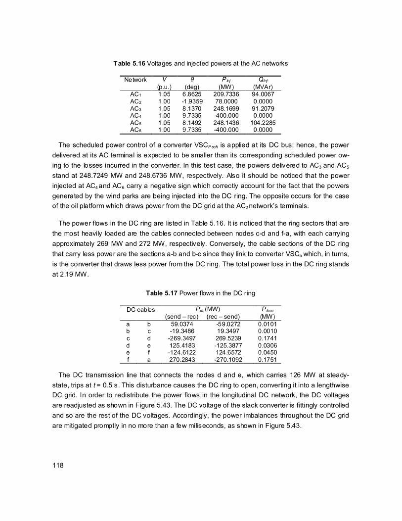
118
Table 5.16 Voltages and injected powers at the AC networks
Network V (p.u.)
θ (deg)
Pinj (MW)
Qinj (MVAr)
AC1 1.05 6.8625 209.7336 94.0067 AC2 1.00 -1.9359 78.0000 0.0000 AC3 1.05 8.1370 248.1699 91.2079 AC4 1.00 9.7335 -400.000 0.0000 AC5 1.05 8.1492 248.1436 104.2285 AC6 1.00 9.7335 -400.000 0.0000
The scheduled power control of a converter VSCPsch is applied at its DC bus; hence, the power
delivered at its AC terminal is expected to be smaller than its corresponding scheduled power ow-
ing to the losses incurred in the converter. In this test case, the powers delivered to AC3 and AC5
stand at 248.7249 MW and 248.6736 MW, respectively. Also it should be noticed that the power
injected at AC4 and AC6 carry a negative sign which correctly account for the fact that the powers
generated by the wind parks are being injected into the DC ring. The opposite occurs for the case
of the oil platform which draws power from the DC grid at the AC2 network’s terminals.
The power flows in the DC ring are listed in Table 5.16. It is noticed that the ring sectors that are
the most heavily loaded are the cables connected between nodes c-d and f-a, with each carrying
approximately 269 MW and 272 MW, respectively. Conversely, the cable sections of the DC ring
that carry less power are the sections a-b and b-c since they link to converter VSCb which, in turns,
is the converter that draws less power from the DC ring. The total power loss in the DC ring stands
at 2.19 MW.
Table 5.17 Power flows in the DC ring
DC cables Pdc (MW) (send – rec) (rec – send)
Ploss
(MW) a b 59.0374 -59.0272 0.0101 b c -19.3486 19.3497 0.0010 c d -269.3497 269.5239 0.1741 d e 125.4183 -125.3877 0.0306 e f -124.6122 124.6572 0.0450 f a 270.2843 -270.1092 0.1751
The DC transmission line that connects the nodes d and e, which carries 126 MW at steady-
state, trips at t = 0.5 s. This disturbance causes the DC ring to open, converting it into a lengthwise
DC grid. In order to redistribute the power flows in the longitudinal DC network, the DC voltages
are readjusted as shown in Figure 5.43. The DC voltage of the slack converter is fittingly controlled
and so are the rest of the DC voltages. Accordingly, the power imbalances throughout the DC grid
are mitigated promptly in no more than a few miliseconds, as shown in Figure 5.43.

119
Figure 5.43 Converter’s DC voltage and power flows in the DC grid
The dynamic behaviour of the modulation ratio of the converters is shown in Figure 5.44, where
it is noticed that only a small readjustment took place after the disconnection of the DC transmis-
sion line. This is so to conform to the post-disturbance voltages obtained in the longitudinal DC
network. The frequency of the passive networks fed by the converters VSCb, VSCd and VSCf are
also reported in Figure 5.44. It stands out that the disturbance in the DC grid does not impose se-
vere affectations on the operation of the island AC networks being fed by the corresponding con-
verters.
Figure 5.44 Modulation ratio of the VSCs and frequency of the passive networks fed by VSCb, VSCd, VSCf.
5.4 Conclusions
Various case studies of the developed steady-state and dynamic models of the STATCOM, point-
to-point and multi-terminal VSC-HVDC links have been presented in this Chapter. The dynamic
response of the STATCOM and point-to-point HVDC link has been comprehensively investigated
using a test network widely-used in academic circles such as the New England test system which
comprises 39 nodes. Furthermore, the model of the point-to-point HVDC link itself has been com-
pared, in terms of the dynamic behaviour of its main state variables, against an EMT-type, switch-
0 0.5 1 1.5 20.999
1
1.001
1.002
Time [s]
DC
vol
tage
[p.
u]
VSCa
VSCb
VSCc
VSCd
VSCe
VSCf
0 0.5 1 1.5 2
-4
-2
0
2
Time [s]
DC
pow
er [
p.u
]
Pab
Pbc
Pcd
Pde
Pef
Pfa
0.858
0.86
Mod
ula
tion
ind
ices
VSCa
VSCc
VSCe
0 0.5 1 1.5 20.79
0.8
Time [s]
VSCb
VSCd
VSCf
0 0.5 1 1.5 249.995
50
50.005
50.01
Time [s]
Fre
quen
cy [
Hz]
VSCb
VSCd
VSCf

120
ing-based model for two different applications; one where the VSC-HVDC link is used to maintain a
scheduled DC power transfer and the other where the VSC-HVDC link is providing frequency sup-
port to low-inertia AC networks. In both cases, it was corroborated that the models are suitable for
conducting both steady-state and dynamic simulations since the state variables’ dynamic response
of the developed models and those of the EMT-type models agree well with each other. The con-
clusions drawn from these validation tests were very much the same when a comparison of a
three-terminal VSC-HVDC system using the developed modelling framework was carried out
against an EMT-type model assembled in Simulink. However, it was also revealed that very signifi-
cant time reductions are obtained when using the proposed RMS-type models developed in this
research work. Undoubtedly, both situations are the result of the comprehensive VSC models to-
gether with their suitable control strategies and the adopted phasorial approach together with the
unified frame-of-reference which is the computing engine that permits an efficient numerical solu-
tion of the models.

121
6 General conclusions and future research work
6.1 General conclusions
The research work reported in this thesis advances current knowledge in the modelling of the
STATCOM, back-to-back and point-to-point VSC-HVDC links and multi-terminal VSC-HVDC sys-
tems aimed at power flows and time-domain, dynamic simulations of electrical power systems. The
starting point is the development of a comprehensive model of the VSC, this being the basic build-
ing block with which the STATCOM, two-terminal and multi-terminal VSC-HVDC links are assem-
bled. These models are useful to carry out steady-state and dynamic simulations of AC/DC net-
works, with the AC networks represented by their positive-sequence equivalents, using phasorial
information.
From the outset, the emphasis of the research work was placed on the realisation of a VSC
model which would capture the essential steady-state and dynamic characteristics of the actual
equipment. This required a fundamentally different modelling approach to the classical VSC repre-
sentation which uses an idealised controllable voltage source (or current source) and quite clearly,
do not possess an explicit DC node. To circumvent this problem, the VSC model put forward in this
research uses a compound phase-shifting transformer and an equivalent shunt admittance with
which key control properties of PWM-based converters may be linked. The phase-shifting trans-
former decouples, angle-wise, the circuits connected at both ends of the ideal complex transformer
in such a way that a notional DC side and AC side of the converter model are created. The equiva-
lent shunt admittance is responsible for the VAR absorption/generation process of the converter to
provide, for instance, voltage control during steady-state operation. This two-port circuit of the VSC,
with its DC and AC sides explicitly available, results in a flexible building block which underpins, in
quite a natural manner, the back-to-back, point-to-point and multi-terminal VSC-HVDC systems for
cases of both, steady-state and dynamic operating regimes. This has resulted in a number of key
improvements in the VSC’s representation: (i) the switching and conduction losses are included in

122
the model in quite a natural manner; (ii) the tap magnitude of the phase-shifting transformer is di-
rectly associated to the amplitude modulation index of the converter; (iii) the DC bus of the con-
verter may be directly connected to, say, another VSC, back-to-back, or by using the model of a
DC cable giving rise to a point-to-point VSC-HVDC configuration; (iv) in fact, any number of these
converter models may be interlinked with ease at their DC buses, to constitute a multi-terminal
VSC-HVDC scheme. Moreover, the VSC model was made more realistic by adding an AC phase
reactor, an AC filter capacitor and an interfacing OLTC transformer on its AC side and, on its DC
side, a shunt capacitor and a series smoothing inductor with its resistive part included. The full
model of the VSC unit and, by extension, its derived formulations, yields a realistic representation
of this equipment even though they are lumped-type models. Their steady-state and dynamic re-
sponses compare well with the responses of the more-detailed, switching-based models available
in EMT-type simulation programs such as Simulink.
A great deal of research effort was paid to the modelling of the back-to-back and point-to-point
VSC-HVDC links, to incorporate realistic control mechanisms. Each one of these two-terminal
VSC-HVDC models was endowed with four degrees of freedom, a feature that conforms well with
actual installations, i.e., simultaneous voltage control on the two AC terminals, DC bus voltage
regulation and regulation of the transmitted power through the DC link. The VSC-HVDC link was
modelled bearing in mind the standard HVDC application of transmitting a scheduled DC power
transfer, the steady-state and dynamic operating regimes were considered. This was followed by
adapting the model to encompass the particular application when the VSC-HVDC link feeds into
passive, near-zero inertia AC networks; the aim was to provide frequency support to weak AC
networks and, accordingly, power flows and dynamic simulations were considered. It should be
brought to attention that its effective participation in frequency regulation was possible owing to the
frequency control scheme in use, which is based on the regulation of the angular aperture that
exists between the internal phase-shifting angle of the rectifier and the voltage angle at its AC ter-
minal. This was amenable to power flow regulation in the DC link and, hence, to frequency control
in the supported AC network, where it was shown that the inverter acts as a virtual synchronous
generator, with its AC bus playing the role of the reference node for all the other nodes in the low-
inertia AC network. The control scheme was comprehensively investigated using a wide range of
gains of the frequency controller, demonstrating its great effectiveness owing to the fast speed of
response of the rectifier station of the VSC-HVDC link, which is in the range of a few milliseconds.
These developments were taken as springboard to tackle the most challenging topic of multi-
terminal VSC-HVDC systems, where a generalised frame-of-reference has emerged that greatly
improves on existing multi-terminal VSC-HVDC models. The proposed frame-of-reference to carry
out steady-state and dynamic solutions of multi-terminal VSC-HVDC systems uses a modular
building block which represents the fundamental-frequency operation of a VSC unit. The dynamic
frame-of-reference is fitted with three different VSC dynamic models (control strategies) applicable
123
to each pairing AC sub-network, namely, the slack converter whose aim is to control its DC voltage,
the scheduled-power converter which injects a scheduled amount of power and the passive con-
verter which is connected to an AC network with no frequency control equipment. The model of the
multi-terminal VSC-HVDC system was tested using a three-terminal scheme and a six-terminal
scheme. The former was used to carry out a comprehensive comparison against an EMT-type
model exhibiting similar characteristics, to demonstrate that the RMS-type model resembles to
switching-based models in terms of the accuracy of its internal variables’ responses for the steady-
state and dynamic operating regimes. The larger multi-terminal VSC-HVDC system has demon-
strated the principle that this new framework is suitable for solving AC/DC power systems where a
single or multiple perturbations at any of the AC networks or at the DC network may occur.
Concerning the numerical solution of these models, the Newton-Raphson method was used as
the computing engine with which the whole set of algebraic and discretised differential equations
were solved, for efficient iterative solutions of the steady-state and operating regimes. The model-
ling approach used to encompass the STATCOM, back-to-back and point-to-point HVDC links and
multi-terminal HVDC systems was a unified framework; one that suitably accommodates and
solves, in a simultaneous manner, all the equations resulting from the VSC-based devices together
with the AC sub-networks. The flow chart presented in Chapter 3, Fig. 3.8, summarizes the adopt-
ed modelling approach for the RMS-type models of the STATCOM and VSC-HVDC models for
both variants steady-state and dynamic operating regimes. In general terms and using case stud-
ies, it has been demonstrated that the new framework enables the comprehensive assessment of
the main operational variables of the VSC-FACTS and VSC-HVDC equipment as well as the study
of the impact of these equipment on the AC and DC networks.
6.2 Future research work
The applicability of the STATCOM, back-to-back, point-to-point and multi-terminal VSC-HVDC
models put forward in this research work, has been demonstrated in terms of power-flow studies
and time-domain, dynamic simulations of power systems. It should be expected that given the high
modularity exhibited by these models, they would be extended to enable their implementation into
other power system analysis tools. For instance:
i. Economic dispatch (ED) and optimal power flows (OPF) are two interrelated tools used to allo-
cate the optimal amount of power that each dispatchable generating unit supplies to the net-
work to ensure minimum generation costs bearing in mind physical and operational constraints.
It is envisaged that the conventional ED and OPF algorithms would need upgrading in order to
incorporate VSC-HVDC models of the two-terminal and multi-termina l kinds. This would enable
124
the study of energy transactions between different AC systems interlinked in an asynchronous
manner.
ii. State estimation of power networks is an application tool that enables the reconstruction of the
state of the whole system, at a given point in time, using partial information coming from in situ
measurement devices. This tool employs positive-sequence, power flow-type models of syn-
chronous generators, wind generators, induction machines, transmission lines, FACTS devices,
etc., to carry out the corresponding state estimations of the power system. In this context, the
steady-state models of the STATCOM and VSC-HVDC systems put forward in this research
work could be used directly to carry out state estimation of AC/DC power networks. Hence, it is
envisaged that the weighted least square method (WLS) could be used, as an initial approach,
to carry out state estimation of AC/DC power systems which would represent a valuable tool
aimed at preserving the stability of the whole system.
iii. The controllability of active power carries high priority in the daily operation of an electrical net-
work; its impact on electrical frequency is direct. Hence, the models of the two-terminal and
multi-terminal VSC-HVDC links could be upgraded to investigate if it is feasible to connect at
any point of the DC network a battery energy storage system. Such a hybrid system has the
potential to provide frequency support to AC networks with embedded VSC-based equipment.
iv. The overall steady-state and dynamic models of the STATCOM and VSC-HVDC systems are
based on power injections (as opposed to current injections), and their solution is carried out,
together with the rest of the power system, using a unified frame-of-reference and Newton’s
method. The Jacobian matrix is readily available at any point in time and this opens a window
of applications for the all-important power systems studies of eigenvalue tracking, dynamic
sensitivity analysis and evaluation of dynamic stability indices. This may be of particular inter-
est to power systems analysts concerned with the security and reliability of the electrical net-
work.

125
References
ABB review special report, special report – 60 years of HVDC (2014). ABB technology Ltd Zur-
ich/Switzerland 2014.
URL:
https://library.e.abb.com/public/aff841e25d8986b5c1257d380045703f/140818%20ABB%20SR
%2060%20years%20of%20HVDC_72dpi.pdf.
Acha E., Fuerte-Esquivel C.R., Ambriz-Perez H. and Angeles-Camacho C. (2005). FACTS model-
ing and simulation in power networks, John Wiley & Sons.
Acha E. and Castro L.M. (2016a). A Generalized Frame of Reference for the Incorporation of Multi-
Terminal VSC-HVDC Systems in Power Flow Solutions, Electric Power Systems Research 136:
415-424.
Acha, E. and Castro, L.M. (2016b). “Power Flow Solutions of AC/DC Micro-grid Structures”. Ac-cepted for publication in the 19th PSCC, Genoa, Italy, on 19-24 June 2016.
Acha E. and Kazemtabrizi B. (2013). A New STATCOM Model for Power Flows Using the Newton-
Raphson Method, IEEE Transactions on Power Systems 28(3): 2455-2465.
Acha E., Kazemtabrizi B. and Castro L.M. (2013). A New VSC-HVDC Model for Power Flows Us-
ing the Newton-Raphson Method, IEEE Transactions on Power Systems 28(3): 2602-2612.
Adam G.P., Ahmed K.H., Finney S.J. and Williams B.W. (2013). Generalized Modeling of DC Grid
for Stability Studies, 4th International Conference Power Engineering, Energy and Electric
Drives (POWERENG), Istanbul, pp. 1168-1174.
Baradar M., and Ghandhari M. (2013). A Multi-Option Unified Power Flow Approach for Hybrid
AC/DC Grids Incorporating Multi-Terminal VSC-HVDC, IEEE Transactions on Power Systems
28 (3): 2376-2383.
Barrios-Martinez E., Angeles-Camacho C., Acha E. and Olguin-Becerril M.A. (2009). Dynamic
Phase-domain Modelling and Simulation of STATCOM in Large-scale Power Systems, IEEE
Power Tech Conference 2009, Bucharest, pp. 1-9.
Bauer J.F., Wissen M., Gutt T., Biermann J., Schäffer C., Schmidt G. and Pfirsch F. (2014). New
4.5 kV IGBT and Diode Chip Set for HVDC Transmission Applications, Power Conversion and
Intelligent Motion (PCIM) Europe 2014, Berlin, pp. 60-67.

126
Beccuti G., Papafotiou G. and Harnerfors L. (2014). Multivariable optimal control of HVDC trans-
mission links with network parameter estimation for weak grids, IEEE Transactions on Control
Systems 22: 676-689.
Beerten J., Cole S. and Belmans R. (2010). A Sequential AC/DC Power Flow Algorithm for Net-
works Containing Multi-terminal VSC HVDC Systems, IEEE PES Winter Meeting 2010, USA,
pp. 1-7.
Callavik E.M., Lundberg P., Bahrman M.P. and Rosenqvist R.P. (2012). HVDC technologies for the
future onshore and offshore grid, Cigré F-75008: 1-6.
Cañizares C.A. (2000). Power flow and transient stability models of FACTS controllers for voltage
and angle stability studies”, IEEE PES Winter Meeting 2: 1447-1454.
Castro L.M., Acha E. and Fuerte-Esquivel C.R. (2013). A New STATCOM Model for Dynamic
Power System Simulations, IEEE Transactions on Power Systems 28(3): 3145-3154.
Castro L.M. and Acha E. (2015a). A novel VSC-HVDC Link Model for Dynamic Power System
Simulations, Electric Power Systems Research 126: 111-120.
Castro L.M. and Acha E. (2015b). On the Provision of Frequency Regulation in Low Inertia AC
Grids Using HVDC Systems, IEEE Transactions on Smart Grid 7(6): 2680-2690.
Castro L.M. and Acha E. (2016). A Unified Modeling Approach of Multi-Terminal VSC-HVDC Links
for Dynamic Simulations of Large-Scale Power Systems, IEEE Transactions on Power Sys-
tems 31(6): 5051-5060.
Chen Q., Tang G. and Wang X. (2005). AC-DC Power Flow Algorithm for Multi-Terminal VSC-
HVDC Systems, Electric Power Automation Equipment 25 (6).
Chaudhuri N.R., Majumder R., Chaudhuri B. and Pan J. (2011). Stability Analysis of VSC MTDC
Grids Connected to Multimachine AC Systems, IEEE Transactions on Power Delivery 26 (4):
2274-2784.
Chiniforoosh S., Jatskevich J., Yazdani A., Sood V., Dinavahi V., Martinez J.A. and Ramirez A.
(2010). Definitions and applications of dynamic average models for analysis of power systems,
IEEE Transactions on Power Delivery 25: 2655-2669.
Chung I.Y., Liu W., Cartes D.A., Collins E.G. and Moon S. (2010). Control methods of inverter-
interfaced distributed generators in a microgrid system, IEEE Transactions on Industrial Appli-
cations 46: 1078-1088.

127
Cole A., Beerten J. and Belmans R. (2010). Generalized Dynamic VSC MTDC Model for Power
system stability Studies, IEEE Transactions on Power Systems 25 (3): 1655-1662.
Cole S. and Belmans R. (2008). Modelling of VSC HVDC using coupled current injectors, IEEE
PES General Meeting - Conversion and Delivery of Electrical Energy in the 21st Century, pp. 1-
8.
Cole S. and Belmans R. (2011). A proposal for standard VSC HVDC dynamic models in power
system stability studies, Electric Power Systems Research 81: 967-973.
Cole S., Karoui K., Vrana T.K., Fosso O.B., Curis J.B, Denis A.M. and Liu C.C. (2011). A European
Supergrid: Present State and Future Challenges, 17th Power Systems Computation Confer-
ence (PSCC) 2011, Stockholm.
Dodds S., Railing B., Akman K., Jacobson B., Worzyk T. and Nilsson B. (2010). HVDC VSC
(HVDC light) transmission - operating experiences, Cigré B4-203 2010: 1-9.
Eghtedarpour N. and Farjah E. (2014). Power control and management in a hybrid AC/DC mi-
crogrid, IEEE Transactions on Smart Grid 5: 1494-1505.
Faisal S.F., Rahim A.H.M.A. and Bakhashwain J.M. (2007). A Robust STATCOM Controller for a
Multi-Machine Power System Using Particle Swarm Optimization and Loop-Shaping, Interna-
tional Journal of Electrical, Computer and Systems Engineering: 64-70.
Fuerte-Esquivel C.R. and Acha E. (1997). A Newton-type algorithm for the control of power flow in
electrical power networks, IEEE Transactions on Power Systems 12: 1474–1480.
Gilje S., Hyttinen M. and Westman B. (2009). Valhall re-development project, power from shore,
Cigré SC B4 2009, pp. 1-10.
Gomis-Bellmunt O., Liang J., Ekanayake J, King R. and Jenkins N. (2011). Topologies of Mul-
titerminal HVDC-VSC Transmission for Large Offshore Wind Farms, Electric Power Systems
Research 81: 271-281.
Gong X. (2012). A 3.3 kV IGBT Module and Application in Modular Multi level Converter for HVDC,
IEEE International symposium on Industrial Electronics ISIE 2012, Hongzhou, pp. 1944-1949.
Guo C. and Zhao C. (2010).Supply of an entirely passive AC network through a double-infeed
HVDC system, IEEE Transactions on Power Electronics 24: 2835-2841.
Hertem D. V. and Ghandhari M. (2010). Multi-terminal VSC-HVDC for the European Supergrid:
obstacles, Renewable and Sustainable Energy Reviews 14: 3156-3163.

128
Hingorani N.G. and Gyugyi L. (1999). Understanding FACTS: Concepts and Technology of Flexi-ble AC Transmission Systems, Wiley-IEEE Press.
Jabbari M., Shahgholian G., Mahdavian M., Attarpour E. and Leilaeyoun A. (2011). Modeling and
Dynamic Analysis of a STATCOM for System Damping Enhancement, IEEE International
Symposium on Industrial Electronics, pp. 1087-1092.
Jacobson B. and Asplund G. (2006). City Infeed with HVDC Light and Extruded Cables, 16th
Conference of the Electric Power Supply Industry, Mumbai, India.
Kjaer S.B., Pedersen J.K. and Blaabjerg F. (2005). A Review of Single-Phase Grid-Connected
Inverters for Photovoltaic Modules”, IEEE Transactions on Industrial Applications 41 (5): 1292-
1306.
Larsson T., Edris A., Kidd D. and Aboytes F. (2001). Eagle Pass Back-to-Back Tie: a Dual Purpose
Application of Voltage Source Converter technology, IEEE Power Engineering Society 3: 1686-
1691.
Latorre H.F., Ghandhari M. and Söder L. (2008). Active and reactive power control of a VSC-
HVDC, Electric Power Systems Research 78: 1756-1763.
Li X., Yuan Z., Fu J., Wang Y, Liu T., and Zhu Z. (2014). Nanao multi-terminal VSC-HVDC project
for integrating large-scale wind generation, IEEE PES General Meeting 2014, National Harbor
MD, USA, pp. 1-5.
Mahdavian M. and Shahgholian G. (2011). Effect of STATCOM on Enhancing Power System Dy-
namic Stability, 8th IEEE International Conference on Electrical Engineering, Computer, Tele-
communications and Information Technology (ECTI-CON), pp. 780-783.
Moustafa M.M.Z. and Filizadeh S. (2012). A VSC-HVDC model with reduced computational inten-
sity, IEEE PES General Meeting, USA, pp. 1-6.
Nnachi A.F., Munda J.L., Nicolae D.V. and Mabwe A.M. (2013). Stability improvement of a HVDC
transmission link between weak AC systems by multi-terminal scheme, IEEE Conference AF-
RICON 2013.
Orths A., Hiorns A., Van Houtert R., Fidher L. and Fourment C. (2012). The European North Seas
Countries’ Offshore Grid Initiative – The Way Forward, IEEE PES General Meeting, USA, pp.
1-8.

129
Peralta J., Saad H., Dennetiere S. and Mahseredjian J. (2012). Dynamic Performance of Average-
Value Models for Multi-terminal VSC-HVDC Systems, IEEE PES General Meeting 2012, USA,
pp. 1-8.
Petersonn A. and Edris A. (2001). Dynamic Performance of the Eagle Pass back-to-back HVDC
Light Tie, 7th International Conference on AC-DC Power Transmission, London, pp. 220-225.
Robinson J., Jovcic D. and Joos G. (2010). Analysis and Design of an Offshore Wind Farm Using
a MV DC Grid, IEEE Transactions on Power Delivery 25 (4): 2164-2173.
Rocabert J., Luna A., Blaabjerg F. and Rodriguez P. (2012). Control of power converters in AC
microgrids”, IEEE Transactions on Power Electronics 27: 4734-4749.
Ronström L., Hoffstein M.L., Pajo R. and Lahtinen M. (2007). The Estlink HVDC Light Transmis-
sion Systems, CIGRE Regional Meeting - Security and Reliability of Electric Power Systems ,
Tallin, pp. 1-7.
Ruihua S., Chao Z., Ruomei L., and Xiaoxin Z. (2005). VSCs based HVDC and its control strategy,
IEEE PES T&D Conference and Exhibition, pp. 1-6.
Sao C.K. and Lehn P.W., (2008). Control and power management of converter fed microgrids,
IEEE Transactions on Power Systems 23: 1088-1098.
Schauder C., Gernhardt M., Stacey E., Lemak T., Gyugyi L., Cease T.W. and Edris A. (1997). Op-
eration of 100 MVAR TVA STATCOM, IEEE Transactions on Power Delivery 12: 1805-1811.
Shahgholian G., Mahdavian M., Etesami A., Moalem S. and Jabbari M. (2011). Improvement of
Dynamic Behavior and System Stability by Using STATCOM, IEEE International Symposium
on Industrial Electronics, pp. 1057-1062.
Shen L., Wang W. and Barnes M. (2014). The Influence of MTDC control on DC Power Flow and
AC System Dynamic Responses, IEEE PES General Meeting 2014, National Harbor MD, USA,
pp. 1-5.
Smed T., Andersson G., Sheble G.B. and Grigsby L.L. (1991). A new approach to AC/DC power
flow, IEEE Transactions on Power Systems 6: 1238–1244.
Stagg, G.W. and El-Abiad, A.H. (1968). Computer Methods in Power System Analysis, McGraw-
Hill.

130
Stendius L. and Jones P. (2006). The challenges of offshore power system construction - bringing
power successfully to Troll A, one of the worlds largest oil and gas platform, 8th IEE Interna-
tional Conference on AC and DC Power Transmission, pp. 75–78.
Teeuwsen S.P. (2009). Simplified dynamic model of a voltage-sourced converter with modular
multilevel converter design, IEEE PES Power Systems Conference and Exposition PSCE,
pp.1-6.
Trötscher T., Korpås M. and Tande J.O. (2009). Optimal Design of Subsea grid for Off-Shore Wind
Farms and Transnational Power Exchange, EWEC2009 Scientific proceedings: European
Wind Energy Conference & Exhibition, pp. 163-167.
Van der Meer A.A., Gibescu M., Van der Miejden M.A.M.M., Kling W.L. and Ferreira J.A. (2015).
Advanced Hybrid Transient Stability and EMT simulation for VSC-HVDC Systems, IEEE Trans.
on Power Delivery 30 (3): 1057-1066.
Vrana T.K., Torres-Olguin R.E., Liu B. and Haileselassie T.M. (2010). The North Sea Super Grid –
A Technical Perspective, 9th IET International Conference on AC and DC Power Transmission,
pp. 1-5.
Wang K. and Crow M.L. (2011). Power System Voltage Regulation via STATCOM Internal Nonlin-
ear Control, IEEE Transactions on Power Systems 26: 1252-1262.
Wang W. and Barnes M. (2014). Power Flow Algorithms for Multi-Terminal VSC-HVDC with Droop
Control, IEEE Transactions on Power systems 29 (4): 1721-1730.
Watson N.R. and Arrillaga J (2007). Incorporation of VSC Transmission in Power-Flow Simula-
tions, 8th International Power Engineering Conference, Singapore, 3-6 Dec, pp. 619-624.
Yao M. and Cai X. (2015). Preliminary study on voltage level standardization of DC grid based on
VSC-HVDC technology in China, IEEE PowerTech Eindhoven 2015, pp. 1-4.
Ye F., Wei Z.N. and Sun G.Q. (2011). Improved Power Flow Algorithm Incorporating Multi-
Terminal VSC-HVDC, ICMST2011 Advanced Materials Research 383-390: 2188-2194.
Zhang L., Harnefors L. and Nee H.P. (2011). Modeling and control of VSC-HVDC links connected
to island systems, IEEE Transactions on Power Systems 26: 783-793.
Zhang X.P. (2004). Multiterminal Voltage-Sourced Converter-Based HVDC Models for Power Flow
Analysis, IEEE Transactions on Power Systems 19: 1877-1884.

ISBN 978-952-15-3866-7ISSN 1459-2045
Tampereen teknillinen yliopisto PL 52733101 Tampere
Tampere University of TechnologyP.O.B. 527FI-33101 Tampere, Finland