


Modelling of mass transfer in gas-liquid stirred tanks ... · Loughborough University Institutional...
50
•
Transcript of Modelling of mass transfer in gas-liquid stirred tanks ... · Loughborough University Institutional...
Loughborough UniversityInstitutional Repository
Modelling of mass transferin gas-liquid stirred tanksagitated by Rushton turbine
and CD-6 impeller: ascale-up study
This item was submitted to Loughborough University's Institutional Repositoryby the/an author.
Citation: GIMBUN, J., RIELLY, C.D. and NAGY, Z.K., 2009. Modelling ofmass transfer in gas-liquid stirred tanks agitated by Rushton turbine and CD-6impeller: a scale-up study. Chemical Engineering Research and Design, 87 (4),pp. 437-451
Additional Information:
• This article was published in the journal, Chemical Engi-neering Research and Design [ c© The Institution of Chem-ical Engineers ] and the definitive version is available at:http://www.elsevier.com/wps/find/journaldescription.cws_home/713871/description#description
Metadata Record: https://dspace.lboro.ac.uk/2134/4950
Version: Accepted for publication
Publisher: Elsevier / c© The Institution of Chemical Engineers
Please cite the published version.

This item was submitted to Loughborough’s Institutional Repository (https://dspace.lboro.ac.uk/) by the author and is made available under the
following Creative Commons Licence conditions.
For the full text of this licence, please go to: http://creativecommons.org/licenses/by-nc-nd/2.5/

1
Modelling of Mass Transfer in Gas-Liquid Stirred Tanks Agitated by Rushton Turbine and CD-6 Impeller: A Scale-up Study
J. Gimbun, C. D. Rielly*, Z. K. Nagy
Dept. Chemical Engineering, Loughborough University, Leics, LE11 3TU, UK.e-mail: [email protected]
Abstract. A combined computational fluid dynamics (CFD) and population balance model (PBM)
approach has been applied to the simulation of gas-liquid stirred tanks agitated by (i) a Rushton
turbine or (ii) a CD-6 impeller, operating at aeration numbers from 0.017 to 0.038. The multiphase
simulations were realised via an Eulerian-Eulerian two-fluid model and the drag coefficient of
spherical and distorted bubbles was modelled using the Ishii-Zuber equations. The effect of the void
fraction on the drag coefficient was modelled using the correlation by Behzadi et al. (2004). The local
bubble size distribution was obtained by solving the PBM using the quadrature method of moments
(QMOM). The local kLa was estimated using both the Higbie penetration theory and the surface
renewal model. The predicted gas-liquid hydrodynamics, local bubble sizes and dissolved oxygen
concentration were in good agreement with experimental measurements reported in the literature. A
slight improvement in the prediction of the aerated power number was obtained using the non-uniform
bubble size distribution resulting from the coupled CFD-PBM simulation. Evaluation of the
prospective scale-up approaches indicates a higher probability of maintaining a similar level of mass
transfer in a larger tanks by keeping the Pg/V and VVM constant. Considering its predictive
capability, the method outlined in this work can provide a useful scale-up evaluation of gas-liquid
stirred tanks.
Key words: gas-liquid; mass transfer; local bubble size; QMOM; CD-6; scale-up; CFD-PBM
1. INTRODUCTION
There are many industrial processes that involve gas-liquid dispersion in stirred tanks, e.g. in
fine-chemicals manufacturing, or in biochemical fermentations. For economic and safety
reasons, reliable models are needed for the scale-up and design of such reactors. One of the
most important problems in modelling gas-liquid dispersions is the prediction of bubble size
and gas-liquid interfacial area. As shown experimentally by many researchers (e.g. Montante
et al., 2008; Barigou and Greaves, 1992; Laakkonen et al. 2005; 2007a) the distribution of
bubble sizes varies inside the stirred tank depends on the spatial position. Generally, bubble

2
sizes around the impeller discharge stream are the smallest due to breakage caused by high
local energy dissipation rates. Furthermore, knowledge of bubble sizes is necessary in a two-
phase CFD model to calculate momentum exchange by drag. Hence, the population balance,
phase continuity and momentum equations are coupled and should in principle be solved
simultaneously. In addition, local bubble sizes and the local gas volume fraction are required
for the calculation of the interfacial area, which is an important variable in designing an
aerated stirred tank to achieve a required rate of gas-liquid mass transfer.
Many modelling studies on the gas-liquid stirred tanks have been performed in recent
years, mostly using a uniform, mono-dispersed bubble size throughout the tank (e.g. Khopkar
and Ranade, 2006; Sun et al., 2005; Wang et al., 2006; Morud and Hjertager, 1996; Deen et
al., 2002; Scargiali et al., 2007). Generally, the CFD predictions of gas hold-up and mean
flow are in fair agreement with experimental data, except around the impeller discharge.
Previous studies have applied a variety of methods with uniform bubble sizes such as grid
refinement, different drag laws and various turbulence models, but without complete success.
Deen et al. (2001) evaluated the effects of different drag laws and grid refinement and found
good predictions of the mean radial velocity but poor predictions of the gas axial velocity.
Others such as Sun et al. (2005) and Wang et al. (2006) employed a k--Ap turbulence model
without a complete success in predicting the two-phase flow. Scargiali et al. (2007) studied
the influence of turbulent dispersion force, virtual mass, grid refinement and the prescribed
bubble size on the holdup in a gas-liquid flow. They concluded that the grid size may
significantly affect the prediction, but effects of the turbulent dispersion force and virtual
mass were not very significant in determining the distribution of gas holdup. Khopkar and
Ranade (2006) studied a gas-liquid stirred tank operating at different flow regimes and
obtained a reasonable predictions of the gas hold-up and gassed power number, but only by
employing the turbulent drag correlations by Brucato et al. (1998): their work showed over
prediction of gas hold-ups around the lower and upper circulation loops.
Whereas it is possible to predict correctly the mean flow in a single phase stirred tank
using any RANS based turbulence model, this performance has not yet been replicated for
gas-liquid stirred tanks. The common practice of employing a uniform bubble size throughout
the tanks is suspected to be the main reason for the poor prediction of the two-phase flow in
stirred tanks. Of course, other factors such as the drag model for distorted and dense bubbles,
turbulent drag laws, lift and other forces also cannot be ruled out. However, their effects
appear to be secondary compared to that of an assumed uniform bubble size on the

3
predominant momentum exchange mechanism of inter-phase drag coefficient, which directly
affects the prediction of the local mean velocities and gas hold-up.
Early attempts to predict the local bubble size were performed using the population
bubble density model (BDM) and a one-way coupled approach, e.g. as in the model of Bakker
and Van den Akker (1994). In recent years, a coupled CFD-BDM has been employed to
predict the local bubble size in gas-liquid stirred tanks by Lane et al. (2002, 2005), Kerdouss
et al. (2006) and Moilanen et al. (2008). In most cases, the BDM is reported to give a
satisfactory prediction of the local bubble size, but only by adjusting some of the empirical
constants within the model. This practice is thought to be inappropriate because the model is
unlikely to be fully predictive and hence cannot be applied to cases where the experimental
data are not available. Lane et al. (2005), for example, introduced a correction factor of up to
3.5 for the turbulence dissipation rate, while Kerdouss et al. (2006) adjusted constants in the
breakage and coalescence term in order to get good agreement with measurements reported by
Alves et al. (2002). Lane et al. (2005) argue that the turbulent dissipation rate is not predicted
well by the RANS k-ε turbulence model. However, the correction factor that was applied is
too large, considering the under prediction of turbulent dissipation rate by k-ε model is only
around than 30% (Ducoste and Clark, 1999). The formulation of the BDM itself is also
questionable, since proper bubble breakage and coalescence kernels are not included. Instead
all equations related to the bubble size are lumped together as a function of the critical Weber
number and energy dissipation rate, without considering the probability and rate of bubble-
bubble and bubble-eddy collisions. As a consequence, the BDM is not thought to be a fully
predictive model for simulation of gas-liquid dispersions in stirred vessels.
A full PBM has been employed to predict the local bubble size in stirred tanks, mostly
using a discretisation based on the method of classes (MOC). Venneker et al. (2001)
performed a one-way coupled PBM via MOC for a stirred tank bioreactor. Recently, a
coupled CFD-PBM simulation using the MOC also has been performed by Montante et al.
(2008), Moilanen et al. (2008) and Kerdouss et al. (2008). Moilanen et al. (2008) showed
reasonable agreement for the predicted and measured local bubble size, based on fitted model
constants in the breakage and coalescence terms from a previous multi-block study. Montante
et al. (2008) presented a good prediction of the number mean bubble size without adjusting
the constants of the kernels, however the Sauter mean diameter was consistently
underpredicted by approximately 50%. No comparison on the predicted bubble size were
presented by Kerdouss et al. (2008). A fully predictive model should not require the tuning of
model parameters for each case considered. One downside of the MOC is its computational
4
demand since it requires more than 30 classes to get a good level of accuracy in the prediction
of the evolution of the moments of the bubble size distribution.
The quadrature method of moments (QMOM) is based on solving equations for the
moments of the bubble size distribution; the quadrature approximation overcomes the
difficulties in obtaining a closed form solution for population balance equations involving
breakage and coalescence. The QMOM requires considerably less computational effort than
the MOC and also is capable of providing an accurate prediction with a relatively small
number of quadrature points. Hence it is suitable for coupling with simulations of the two-
phase hydrodynamics. The QMOM has been applied previously to breakage and aggregation
problems (e.g. Marchisio et al., 2003). Recently, Petitti et al. (2007) have employed the
QMOM to solve the bubble dynamics for gas-liquid dispersion. In their work, bubble
coalescence is not considered and only a simple breakage kernel is employed instead of one
based on the physics of bubble breakup. No comparisons with experimental measurement
were presented by Petitti et al. (2007). In the interest of a reduced computational effort, the
QMOM method was selected to solve the population balance equation for bubble dynamics in
aerated stirred tanks in this work.
The first part of this work focuses on the development of a modelling approach for gas-
liquid stirred tanks. For an initial comparison, the CFD simulation was performed assuming a
constant bubble size throughout the tank. A coupled CFD-PBM was then performed to
account for the spatially non-uniform bubble sizes inside the tank. The CFD prediction of the
two-phase flow field was compared to experiments by Deen et al. (2002), whereas the results
using the CFD-PBM approach were compared against measurements by Laakkonen et al.
(2007a and b). After validation, the model was used to evaluate the local mass transfer
coefficients inside the tank, and to study the reactor scale-up, especially from the mass
transfer perspective, which is often vital in aerobic fermentations.
2. MODELLING APPROACH
2.1 CFD modelling of two-phase flow
The Eulerian-Eulerian approach is employed for gas-liquid stirred tanks simulation in this
work, whereby the continuous and disperse phases are considered as interpenetrating media,
identified by their local volume fractions. The volume fractions sum to unity and are
governed by the following continuity equations:
5
0
lllll ut
(1)
where αl is the liquid volume fraction, ρl is the density, and lu
is the velocity of the liquid
phase. The mass transferred between phases is negligibly small and hence is not included in
the right hand-side of eq.(1). A similar equation is solved for the volume fraction of the gas
phase by replacing the subscript l with g for gas. The momentum balance for the liquid phase
is:
lvmlliftlllllllllll FFgFPuuut ,,lg
(2)
where l is the liquid phase stress-strain tensor, lliftF ,
is a lift force, g
is the acceleration due
to gravity and lvmF ,
is the virtual mass force. A similar equation is solved for the gas phase.
lgF
is the interaction force between phases, mainly due to drag. As pointed out by Scargiali et
al. (2007) the effects of the turbulent dispersion, virtual mass and lift are almost negligible,
despite a significant increase in computational expenses and convergence difficulties.
Scargiali et al. (2007) found a minimal increase of the overall gas hold-up from 4.36% to
4.60% and from 4.36% to 4.67% by adding the effect of virtual mass and lift force
respectively. They concluded that the effect of the drag force largely predominates in aerated
stirred tanks. A similar conclusion was also drawn by many previous studies, e.g. Bakker and
Van Den Akker, 1994; Morud and Hjertager, 1996; Lane et al., 2002; Kerdouss et al., 2006).
It was therefore decided not to include the effect of the virtual mass and lift force in this work.
Hence, lgF
is represented by a simple interaction term for the drag force, given by:
b
lglgDlgl
d
uuuuCF
4
3lg
(3)
where CD is a drag coefficient and db is the Sauter mean bubble diameter.
The drag model employed has a significant effect on the flow field of the aerated flow, as
it is related directly to the bubble terminal rise velocity. Bubbles have a tendency to form a
non-spherical shape, especially those with a diameter > 3 mm. Therefore, the drag model of
Ishii and Zuber (1979) was selected in this work, as it takes into account the drag of distorted
bubbles:
38,
3
2min,Re15.01
Re
24max 687.0
Obb
D EC (4)

6
where the Reb and EO are the bubble Reynolds number and Eotvos number, respectively. The
drag for the ellipsoidal bubble regime is dependent on the bubble shape through the Eotvos
number, which represents the ratio of gravitational to surface tension forces; for the spherical
cap regime the drag coefficient is approximately 8/3. The effect of the local bubble volume
fraction on the drag coefficient is estimated using Behzadi et al.’s (2003) correlation as
follows:
864.064.3, eCC DdenseD (5)
where the CD is the drag coefficient for isolated bubble estimated using eq.(4), whereas
denseDC , is for the dense dispersion of bubbles. The drag model described above is not
available as a standard option in FLUENT and hence it has been implemented via a user-
defined subroutine.
The stirred tank grid was prepared with a headspace to accommodate liquid expansion
due to aeration. The liquid surface was modelled as a freely expandable liquid surface and the
top of the headspace region was set as a pressure outlet, rather than using a fictitious
‘degassing boundary condition’. The mass balance between the gas outflow at the outlet
boundary (above the headspace region) and the gas inflow at the sparger was satisfied. The
PBM and mass transfer calculations did not include the headspace region.
It is also important to consider the formation of the bubble cavity behind the impeller
blade. According to Lane et al. (2005), it is possible to model the gas cavity in the Eulerian-
Eulerian framework, providing a certain modification is made to the interphase exchange
coefficient: the drag coefficient is set to turn into that for isolated bubble when the void
fraction is higher than 0.7, i.e. the cavity behind the blade behaves in a manner similar to an
isolated bubble, rather than the dense bubble case. An attempt to use the dense drag bubble
model for the cavity region has been tested, resulting in the disappearance of the bubble
cavity behind the blade and an over-prediction of the gassed power number by more than
60%. The mean radial velocity was also found to be over predicted. However, this issue has
been successfully addressed by treating the cavity as an isolated bubble.
2.2 Turbulence modelling
The turbulence modelling uses the two-phase realizable k- model, in which both k and
are allowed to have different values for each phase. The transport equations for the realizable
two-phase k-ε model are given in the Fluent manual (2006) and the standard values of the
model parameters have been applied. The realizable k-ε is considered to be a better model

7
than the standard k-ε for stirred tank flows (Gimbun, 2009), as it better accounts for flow
features such as strong streamline curvature, vortices and rotation. The realizable k-ε differs
from the standard k-ε model in two important ways: first it has a new formulation of turbulent
viscosity and second it employs a new transport equation for the dissipation rate incorporating
different model constants.
2.3 Population balance modelling
2.3.1 QMOM formulation
The QMOM is employed to solve the PBM and predict the evolution of the moments of the
bubble size distribution. For breakage and coalescence only, the QMOM equation for the kth
moment of a single well-mixed system is given by:
ecoalescenctoduedeath
1 1
breakagetoduedeath
1
ecoalescenctoduebirth
1
3/33
1
breakagetoduebirth
1
,
,2
1,
d
d
N
i
N
jjij
kii
N
i
kiii
N
jji
kjij
N
ii
N
iiii
k
LLwLwLLaw
LLLLwwLkbLawt
(6)
where ji LL , , a(Li) and iLkb , are the coalescence kernel, breakage kernel and daughter
bubble distribution function, respectively. Full details of the QMOM can be found elsewhere
e.g. McGraw (1997) and Marchisio et al. (2003). In this implementation, the solution of the
weights (w) and abscissas (L) from the moments was obtained using the product difference
algorithm of Gordon (1968). To reduce computation cost of these simulations a QMOM
based on two quadrature points was applied.
There are many breakage and coalescence kernels available for bubbly flow, but they are
essentially written in a similar form except some minor differences in the model constants or
assumptions. The Prince and Blanch (1990) model has been proven to give a good prediction
of bubble size in bubble columns (e.g. Shimizu et al., 2000; Podila et al., 2007). Some
researchers (e.g. Chen et al., 2005; Bordel et al., 2006; Podila et al., 2007) made a
comparison of the prediction of various kernels combinations including those proposed by
Prince and Blanch (1990), Luo and Svendsen (1996), Luo (1993), Chesters (1991), Martinez-
Bazan et al. (1999) and Lehr et al. (2002). Their findings suggest that there is no great
difference between the mean flow, gas hold-up and bubble Sauter mean diameter (d32)
predicted using different kernels although, there are some differences in the predicted bubble
size distribution. The Luo and Svendsen (1996) breakup kernel was found to generate
8
excessively small and large bubbles, due to its U-shaped daughter bubble distribution function
(Podila et al., 2007). Podila et al. also pointed out the problem of the Luo (1993) coalescence
kernel, which tends to yield large bubbles due to its high coalescence rates. Laakkonen et al.
(2007a) and Moilanen et al. (2008) employed a modified version of Prince and Blanch’s
(1990) model for their work on gas-liquid stirred tanks, and they reported a good agreement
with experimental measurement. Laakkonen et al. (2007a) has compared the prediction of two
different kernels i.e. Lehr et al. (2002) and a modified version of Prince and Blanch models.
Their findings suggest that Lehr model tends to under predict the local bubble size in gas-
liquid stirred tanks, even though it has been reported to produce an excellence prediction for
bubble columns (Lehr et al., 2002). Based on these previous studies, the Prince and Blanch
(1990) model has been employed to predict the bubble dynamics in this work.
2.3.2 Modelling of bubble coalescence
Bubble collisions may occur due to a variety of mechanisms, e.g. Prince and Blanch (1990)
consider collisions arising from turbulence, buoyancy and laminar shear. In turbulent flow,
bubble collisions are driven mainly by random motion of bubbles due to turbulent eddies.
Bubbles of different sizes also have different rise velocities which may lead to collision.
There is also a possibility for bubbles from a high liquid velocity region to collide with
bubbles in slower section of the velocity field. The bubble collision frequency for a
Newtonian fluid can be modelled following the approach proposed by Prince and Blanch
(1990):
bouyancy
jiji
turbulent
jtitji
ji LuLuLL
LuLuLL
LL )()(22
)()(22
,2
5.022
2
(7)
where ut (L) is the turbulent velocity in the inertial range of isotropic turbulence (Rotta, 1972)
and u (Li) is the rise velocity of bubble given as a function of bubble size (Clift et al., 1978).
The bubble collision efficiency, ji LL , , is the probability of coalescence during a
bubble-bubble collision between sizes Li and Lj. For Prince and Blanch’s model, the bubble
collision efficiency is given as a function of film drainage and bubble-bubble contact times:
3/13/2
3
/2/
16/2/lnexp,
ij
lijfo
jiL
LhhLL (8)

9
where 1112 jiij LLL , ho is the initial film thickness and hf is the final thickness at which
the film rupture occur. The value of 10-4 m for ho and a value of 10-8 m for hf from Prince and
Blanch (1990) was used throughout this work. The bubble coalescence kernel, ji LL , , is a
product of bubble collision efficiency, from eq.(7), and collision frequency from eq.(8).
jijiji LLLLLL ,,, (9)
2.3.3 Modelling of bubble breakage
Prince and Blanch (1990) considered the bubble break-up to be caused by collisions with
turbulent eddies of sizes equal to, or smaller than, the bubble size. They argued that eddies
smaller than 0.2 times the bubble diameter are unlikely to contribute significantly to the
overall break-up rate and set the lower limit of the effective turbulent eddies as 0.2L. They
considered only eddies having a velocity larger than the critical velocity, uci, where the
disruptive force due to the kinetic energy of the eddy and the cohesive force due to surface
tension balance each other. The break-up rate is given as a product of the collision rate of
bubbles with turbulent eddies, ie , and the break-up efficiency, i . According to Prince and
Blanch (1990), the bubble break-up rate is given by the expression:
iieiLa (10)
The collision rate of bubbles with turbulent eddies is given by Kennard (1938):
5.022tetiieeiie uuSnn (11)
where ni, ne and Sie are the number of bubbles per unit volume, number of eddies per unit
volume and collision cross-sectional area, respectively. The uti is the turbulent velocity in the
inertial range of isotropic turbulence (Rotta, 1972) and the eddy velocity, ute, of a size Le is
also calculated analogously to Rotta (1972). The eddy size may be expressed using
Kolmogorov’s (1941) theory of isotropic turbulence as 4/13 le vL .
The break-up efficiency, i , is given by (Kennard, 1938; Prince and Blanch, 1990):
22exp tecii uu (12)
where the uci is the critical eddy velocity necessary to break a bubble of diameter Li, given by
Shimizu et al. (2000).
Prince and Blanch’s (1990) break-up model does not include the daughter bubble size
distribution. The daughter bubble distribution function, ,Lb , determines the number and

10
size of the daughter particle, L, after the breakage event of particle size . Here, a uniform
breakage function was selected with binary breakage to form similar particle sizes.
3
26|
L
Lb (13)
There is a high possibility of non-binary breakage for liquid-liquid systems where the
internal viscosity of the dispersed phase can lead to multiple daughter drops (Andersson and
Andersson, 2006). However the assumption of binary break-up is considered valid for
bubbles, since the air viscosity is low. Furthermore, a recent study by Andersson and
Andersson (2006) revealed that more than 95% of bubble break-ups involved binary
breakage.
The population balance model was solved using user-defined scalars to represent the
moments, weights and abscissas and was implemented via user-defined subroutine written in
C language. All the breakage and coalescence kernel were implemented without adjusting any
of the model constants. The user-defined subroutine was compiled within the commercial
CFD code, FLUENT 6.3 and was available as an add-on program after the compilation; hence
a fully coupled CFD-PBM simulation could be performed.
2.4 Modelling of kLa and oxygen transfer rate
Many empirical scale-up rules and correlations have been developed to calculate the
volumetric mass transfer coefficient, kLa, in aerated stirred tanks. However, the existing
correlations are only capable of calculating the average kLa value in the tank and not the local
values. Information about the local kLa is important in the study of gas-liquid stirred tanks to
spot the occurrence of ‘dead zones’, where very little mass transfer occurs. Ideally, achieving
a uniform kLa and uniform driving force is desirable during scale-up of aerated stirred tanks.
Whilst this maybe the case for laboratory scale stirred tanks, it is not always true for larger
scale tanks, which can suffer from zones of oxygen depletion, particularly where there is an
oxygen sink, e.g. through chemical reaction.
Assuming a spherical bubble, the local interfacial area per unit volume may be calculated
from
i
iib nda 2, (14)
where db,i is the bubble size and ni is number of bubbles of size db,i per unit volume of
dispersion. The bubble sizes and numbers of bubble used in the calculation of the interfacial
area were obtained from the CFD-PBM simulation, directly from the weights and abscissas

11
used in the QMOM. Bubbles with diameters greater than around 3 mm (for air-water) are
ellipsoidal, with an aspect ratio which may be calculated as a function of the Eotvos number
from the correlation of Wellek et al. (1966)
757.0163.01 OER (15)
which was developed originally for liquid–liquid dispersions. Guet et al. (2005) compared
eq.(15) with their experimental measurements obtained using a four-point optical fibre probe
and reported that Wellek et al.’s (1966) correlation is applicable for bubbles. In this work the
interfacial area for small bubble (db ≤ 1 mm) was estimated from eq.(14), whilst the bigger
bubbles (db > 1 mm) were assumed to be as oblate spheroids and their surface area was
calculated using R from eq.(15). Even larger bubbles (db > 5 mm) may not form perfect oblate
ellipsoids in turbulent flow, however, eq.(15) is a step towards improved bubble shape
prediction.
Penetration theory (Higbie, 1935) and the surface renewal model (Danckwerts, 1951) are
two common methods of calculating kL when the bubble size is known. Higbie’s (1935)
penetration theory results in an average mass transfer coefficient for each bubble size given
by:
ib
slipliL d
uDk
,,
2
(16)
where uslip and Dl are the bubble slip velocity and diffusion coefficient, respectively. The slip
velocity can be obtained from the difference in phase velocities from an Eulerian-Eulerian
two-fluid CFD simulation. Thus local values of kLa were calculated from:
i
islipiblL nudDak 5.05.1,
5.0π2 (17)
Danckwerts (1951) suggested a refinement of the penetration model by assuming that kL is
related to the average surface renewal rate resulting from exposure of the bubble interface to
turbulent eddies with a variable contact time. Danckwerts suggested the surface renewal
model as follows:
sDk lL (18)
where s is the fractional rate of surface-element replacement. Lamont and Scott (1970)
assumed that the small scale turbulent motion, which extends from smallest viscous motion to
inertial ones, affects the rate of mass transfer. Consequently, s can be calculated using
Kolmogorov's theory of isotropic turbulence. They suggested the eddy cell model as follows:

12
25.05.0
l
llL v
KDk
(19)
where εl is the turbulence dissipation rate in the liquid phase, vl is the liquid dynamic viscosity
and K = 0.4 is the model constant. Combining kL and a gives another equation for calculating
the volumetric mass transfer coefficient:
iiib
l
llL nd
vDKak 2
,
25.05.0
(20)
The local oxygen transfer rate can be estimated from the following relations once the local
kLa has been determined,
oooLo rCCakN )( * (21)
where *oC is the oxygen solubility in the liquid phase, Co is the oxygen concentration in the
liquid phase and ro is the specific oxygen consumption rate. The transport equation for
dissolved oxygen mass fraction was also solved as a user-defined scalar implemented as a
user-defined subroutine, with the sink terms given in the right had side of eq.(21) above.
2.5 Tank geometry and numerical strategy
Two scales, 14L and 200L, of aerated stirred tanks containing a Rushton turbine, studied by
Laakkonen et al. (2007a) were considered for the CFD-PBM modelling. Gas was injected
through a sparger ring at a flow rate ranging from 0.29 to 0.7 vvm which is treated as a
continuous source of gas (velocity inlet) in the CFD simulation. First, a two-phase CFD
simulation was performed assuming a uniform bubble diameter throughout the tank. The
interphase drag coefficient was estimated using the standard Schiller-Naumann drag model.
The CFD simulation was performed using a half-tank domain consisting of about 225k
hexahedral cells. A finer mesh was employed around the impeller up to 15 nodes placed along
the impeller blade height. According to Derksen et al. (1999), a grid with eight or less nodes
along the impeller blade height may not be able to resolve the vortex core structure correctly
and hence can give errors in the predicted mean flow field. The impeller movement was
modelled using a multiple reference frame and the Eulerian-Eulerian approach was employed
for the multiphase modelling. The turbulence was modelled using the two-phase realizable k-ε
model described in a previous section. Transient solvers with a second-order spatial
interpolation scheme were also applied for the final simulation in order to minimise the
amount of numerical diffusion. The iteration residual was set to fall below 110–4 at each time

13
step to achieve good convergence. The volume average of the gas void fraction at the rotating
zone (impeller region) was also monitored and the iterations were only halted once a constant
value was observed. A grid sensitivity study was performed prior to the final grid selection
using three different meshes: coarse (165k with 6 nodes at impeller blade height),
intermediate (225k with 11 nodes at impeller blade height) and fine (335k with 13 nodes at
impeller blade height). It was found that a domain consisting of 225k cells yielded a grid
independent solution (see Fig. 1).
3. RESULTS AND DISCUSSION
3.1 Prediction of Gas-Liquid Hydrodynamics
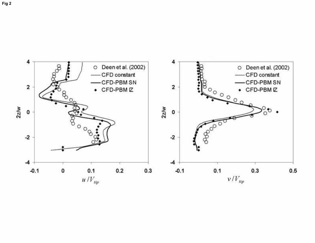
First, the CFD simulations were validated against experimental data using the two-phase PIV
measurements reported by Deen et al. (2002) for a stirred tank with Flg = Qg/ND3 = 0.0296.
The impeller speed for Laakkonen’s geometry was set to 513 rpm to ensure the aeration
number stayed at Flg = 0.0296 so that a sensible comparison between the CFD prediction and
the experimental measurement from Deen et al. (2002) could be made.
The simulation was performed initially by assuming a constant bubble size of 3.5 mm
throughout the tank. The bubbles were assumed to be spherical and the Schiller and Naumann
(1935) drag model was employed to estimate the drag coefficient. The CFD results were time-
averaged over all blade angles and compared with Deen et al.’s (2002) PIV measurements.
For easier comparison, the results for the mean velocities were normalised using the impeller
tip velocity (Vtip). Despite the assumption of a constant bubble size and spherical bubbles, the
predictions (marked as CFD constant) shown in Figs. 2 and 3 are reasonably close to the
experimental data. The differences can be explained by the neglect of bubble coalescence and
break-up caused by the turbulent flow induced by the rotating impeller. These mechanisms
are not considered in the case where a uniform bubble size is assumed throughout the tank.
A simulation using a non-uniform bubble size was next performed to evaluate these effects on
the CFD predictions. The local bubble sizes were estimated using the population balance
model, which tracks the moments of the bubble size distribution. The local Sauter mean
diameters, obtained from the ratio of the third and second moments, were then passed into the
CFD simulation and used for the two-phase flow modelling. The CFD-PBM simulations were
performed using two different drag models: (i) the hard sphere drag model of Schiller and
Naumann (1935) (a default FLUENT model) and (ii) another that takes into account the drag
of distorted bubbles (Ishii and Zuber, 1979) and dense bubble effect (Behzadi et al., 2003). As
expected, results obtained from the CFD-PBM modelling were slightly better compared to

14
those obtained using a constant bubble size. The prediction of axial gas velocities below the
impeller (2z/W < 1) and the peak liquid radial velocities were in fair agreement with Deen et
al.’s (2002) data. Using the non-spherical drag model (CFD-PBM-IZ) in the CFD-PBM
approach further improved the results. This is due to the fact that the effect of local bubble
sizes on the two-phase flow is mainly via the inter-phase exchange coefficient, which
depends on the drag model. The Schiller-Naumann model is suitable for spherical rigid
bubbles, but in comparison, the Ishii-Zuber model predicts drag coefficients for the spherical,
ellipse and cap bubble regime. The difference observed between the flow fields predicted
using a spherical drag model and the one that accounts for distorted bubbles is small for the
cases considered in this paper, due to the proximity of the analysed region to the impeller tip.
In this region, the bubble size is mainly below 3 mm and hence bubbles can be assumed to be
approximately spherical. However, because of the better prediction of the gas and liquid mean
velocities, the CFD-PBM-IZ was selected and used for the remainder of this work. The
remaining discrepancy in the result predicted by CFD-PBM-IZ method might be due to minor
differences in the tank geometry used by Deen et al. (2002) and Laakkonen et al. (2007a) (the
geometry used for the CFD work reported here). For instance Deen et al. (2002) used a dished
bottom tank and had a slightly different impeller geometry (W = LD = 0.25D) whereas
Laakkonen’s work used a flat bottomed tank and a standard Rushton turbine. The inherent
limitation of the Eulerian-Eulerian model which can only use a single bubble size (d32) at any
spatial location at any given time is also thought to affect the accuracy of CFD prediction. A
more accurate modelling approach of the gas-liquid flow would employ the real bubble size
distribution at each spatial position inside the tank, however such model would require a
higher implementation complexity and would be computationally more intensive to run.
Therefore, a combined CFD-PBM model employing only the d32 is thought to be a more
efficient solution for a gas-liquid flow at present with the aim of employing the developed
approach as a practical design tool.
3.2 Prediction of the Aerated Power Number
Prediction of the gassed power input by integrating the dissipation rate over the tank volume
is known to provide an underestimate of the power input (in the cases shown here, by between
35–44 %). Therefore the Pg in this work was calculated from the moment acting on the shaft
and impeller or baffles and tank wall. The calculated torque, , is then related to the power
input by,

15
NPg 2 (22)
For a Rushton turbine Bujalski et al. (1987) suggested the following correlation for
estimation of the ungassed power number:
063.0195.0
530
0 512.2 TD
t
DN
PN
lp
(23)
where t is the impeller thickness and T is the tank diameter (m). Smith (2006) proposed the
following correlation for the relative power draw, Pg/P0, for stirred tanks agitated by a
Rushton turbine, based on the measurements of Warmoeskerken and Smith (1982) and
Gezork et al. (2000):
25.02.00 18.0 gg FlFrPP , (24)
where Fr and Flg are the Froude number and the aeration number, respectively. Myers et al.
(1999) performed extensive experiments in single phase and aerated stirred tank with a CD-6
impeller; they reported that, on gassing, the Pg/P0 of a Rushton turbine drops significantly
compared to that of a CD-6 impeller. In this study the CFD predictions were compared with
measured Pg/P0 obtained from Myers et al. (1999) for the CD-6 impeller, and using eq.(24)
for the Rushton turbine, together with eq.(23).
The Pg/P0 ratio is shown to be predicted reasonably well using the assumption of a
constant bubble sizes throughout the tank (see Tables 1 and 2). There is a small improvement
in the prediction of Pg/P0 when a non-uniform bubble size is employed using the CFD-PBM
method, especially for cases 1, 4, 5 and 6 for which the uniform bubble sizes used for the
initial simulation differed significantly from those calculated using the PBM. The bubble
sizes for cases 2 and 3 were known from Laakkonen et al. (2007a), and mean values were
used for these initial CFD simulations. Consequently, the CFD predictions using uniform
bubble sizes for cases 2 and 3 are much closer to the values estimated from eq.(24). The
results suggest that the Pg/P0 can be predicted reasonably well using the uniform bubble size
assumption with bubble size close to the experimental mean values. However, the CFD-PBM
method is a more suitable approach for predicting the relative power number in cases when
the mean bubble size is not known beforehand.
3.3 Prediction of Local Bubble Size and Mass Transfer Coefficient
CFD-PBM simulations were performed using a user-defined subroutine compiled within
FLUENT. The Prince and Blanch (1990) breakage and coalescence kernels were employed to
predict the bubble dynamics throughout the tank, using literature values of the model

16
constants. The volume-average Sauter mean diameter, d32, in the impeller region was used as
a convergence indicator in these simulations.
Figures 4 and 5 show that the local bubble sizes predicted by the CFD-PBM simulation
for both the smaller and the larger tanks are in good agreement with the experiments by
Laakkonen et al. (2007a). The smallest bubbles can be observed around the impeller, where
the dissipation rates are a maximum, whereas the largest bubbles are found below the
impeller, just above the sparger, due to the combination of a high void fraction and low
dissipation rates. Some discrepancies in the local bubble size predictions can be observed,
possibly due to the well-known under-prediction of the energy dissipation rates by the k-ε
model—the evolution of the bubble size depends mainly on the dissipation rates and the gas
void fraction. The CFD-PBM approach is also capable of responding to changes in operating
conditions. For instance, case 1, which considers a lower impeller speed, produces larger
bubbles compared to case 2, where the impeller speed is higher (see Table 1).
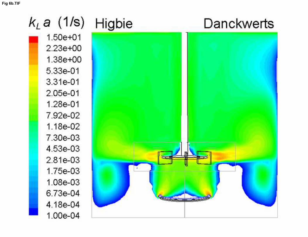
Using the local bubble size obtained, the local kLa can be estimated using Higbie’s
penetration theory, or the surface renewal model of Danckwerts. The latter gave a
significantly higher value of kLa around the impeller region (see Fig. 6) due to its sensitivity
towards high dissipation rates. Higbie’s method return a higher local kLa in the bulk region,
where the dissipation rates were very low; the two methods show slightly different
sensitivities to the local dissipation rate and bubble size. The maximum local kLa values for
the larger tank were significantly smaller (roughly 50% less) than for the smaller tank due to
the larger mean bubble size, which consequently reduced the interfacial area. The local kLa
contour map also revealed a large dead zone in the bottom region of the tank due to the poor
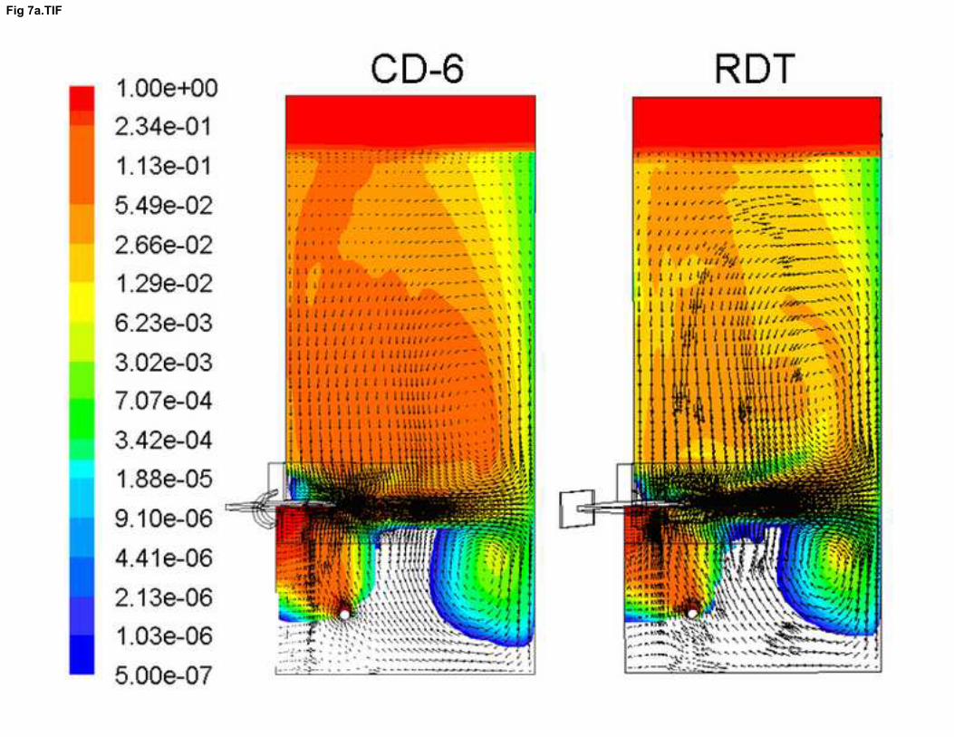
gas dispersion produced by the Rushton turbine. This can be addressed by employing a better
gas dispersion impeller such as the CD-6, as shown in Fig. 7A. The CD-6 impeller is a
concave type impeller which is available commercially from Chemineer and has been studied
extensively by many researchers (e.g. Myers et al., 1999). There are several reason why the
CD-6 disperses bubbles much better than the Rushton turbine. Firstly, the CD-6 pumps the
fluid slightly downward around the impeller discharge region, whereas the Rushton turbine
pumps slightly upward (see Fig. 7A), which then contributes to poor circulation of bubbles in
the lower region. Secondly, the concave shape of the CD-6 is designed to produce a smaller
gas cavity behind the impeller blade (see Fig. 7B) leading to less reduction in the aerated
power number in comparison to the Rushton turbine.

17
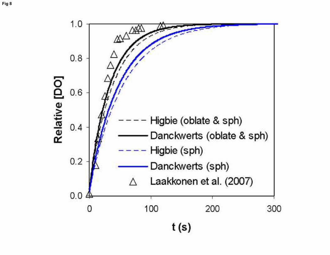
By analogy with experimental measurements, which often assume a well-mixed liquid
phase, a global mean akL was estimated by monitoring the volume-averaged oxygen
concentration, Co(t), throughout the simulation, from
takCC
tCCL
oo
oo
0ln
*
*
(25)
where *oC is the oxygen solubility in water. In the cases discussed here, estimated mixing
times from the correlation by Grenville and Nienow (2004), were about one order of
magnitude greater than 1
akL , indicating the liquid phase was well-mixed. Values of akL
were obtained from the slopes of the graphs obtained by plotting the left hand side of eq.(25)
against time. Fig. 8 shows the evolution of the dissolved oxygen concentration, [DO],
calculated using the Higbie and Danckwerts methods, respectively. The predicted Co(t) profile
is in good agreement with the experimental measurement from Laakkonen et al. (2007b)
especially when an oblate spheroid shape is considered for the larger bubbles. As expected,
the discrepancy is much bigger when bubbles assumed to be in spherical shape throughout the
tank which may not be correct for diameters > 3 mm. Furthermore, the Eulerian-Eulerian
simulation works with a single slip velocity, despite the existence of a range of bubble sizes;
this may introduce some discrepancy in the local kLa and the [DO] evolution. However, this
simplification is necessary in order to keep the computational demand minimal. Moreover, the
two-phase model can get excessively complicated and expensive to compute when individual
bubble sizes with separate slip velocities are considered. Due to its better prediction of the
[DO] evolution, the combined spherical and oblate spheroid model is applied for the
remainder of this work.
Higbie’s method is consistently found to have a slightly faster oxygen transfer rate than
the Danckwerts’s method for a smaller vessel (see Fig. 9A), where the mean bubble size is
less than 3 mm, but the difference becomes almost insignificant for the larger vessels (see Fig.
9B) when the mean bubble size is about 4 mm. This is reflected in the calculated values of
the mean akL shown in Tables 3, for cases 2 and 4. Furthermore, Danckwerts’ model tend
to have a faster oxygen transfer rate than the Higbie model when the mean bubble size is
larger than 5 mm (see Fig. 8). This phenomenon can be explained by the sensitivity of the
Higbie’s model to small bubble sizes which are formed in great numbers for the smaller
vessel.

18
The [DO] evolution was recorded at three different locations inside the tank namely the
dead zone below the sparger, the impeller region and bulk region above the impeller. Only a
small amount of variation was found between the akL value estimated using the [DO]
evolution recorded at these three different locations (see Fig. 10), hence the remaining
discussion focuses only on the data recorded at impeller discharge, where the majority of
experimental measurements have been obtained. In eq. (25), and often in experimental
measurements of the mass transfer coefficient, it is assumed that the dissolved oxygen
concentration, [DO] is uniform. Results from the CFD-PBM simulation suggests that this
assumption is applicable for these lab and pilot scale gas-liquid vessels, without the presence
of oxygen sink (i.e. reaction or micro-organism respiration). It is important to note that, the
assumption of uniform [DO] may not be valid in a gas-liquid bioreactor even at small scale,
depending on the local rate of consumption of dissolved oxygen. In such a case, the [DO] may
fall towards zero in some dead regions leading to a severe mass transfer limitation. The well-
mixed assumption is also less likely to be correct with increasing scale of operations
(Schuetze and Hengstler, 2006), especially when dealing with industrially sized vessels. Thus
in practice, the [DO] may be non-uniform, being almost saturated in some locations where
there is a high local kLa, and having a low [DO] in regions with poor gas dispersion. It may
be concluded that simple volume averages of kLa from CFD simulations, without knowledge
of their correlation with local driving forces, are of little practical use; they would tend to be
larger than the akL values obtained by experiment, or from eq.(25). However, a CFD
calculation which solves the oxygen transport equation, coupled with local values of kLa takes
this effect into account, and can serve as a more correct framework for the design and scale-
up of aerated stirred tanks than methods that use eq.(25) with volume averaged quantities.
Generally, the akL for air-water stirred tanks is given in the following form:
bg
agakL vVPCak
L (26)
For air-water system van’t Riet (1979) suggested a value of akLC = 0.026, a = 0.4 and b = 0.5
obtained from a fit to experimental measurements. These constants have been the subject of
many studies and their values vary from author to author depending on the tank size and gas
loading. The correlations in eq.(26) are reported to be able to predict satisfactorily the akL
of similar size vessels, but they do not necessarily apply for scale-up to an industrially sized
tank (Lines, 2000; Stenberg and Andersson, 1988).

19
Comparison between the akL estimated using the eq.(26) and the model evaluated in
this work (using the [DO] evolution at the impeller region) is presented in Table 3. Higbie’s
model was found to give a closer prediction of akL compared to the value estimated using
eq.(26), while Danckwerts’s model consistently gave a slightly smaller akL value except for
case 5 where the mean bubble size is larger than 5 mm. The relative error from the akL
value obtained from eq.(26) and the CFD simulations ranged from 3% to 35%, with a larger
error shown for the bigger vessel. The correlations in eq.(26) are known to be problematic
when applied to tanks of different size from that of the original experiments. For instance,
Garcia-Cortes et al. (2004) reported a deviation up to 18% from their experimental
measurement; earlier Zhu et al. (2001) reported about 20% discrepancy. The differences in
the CFD simulations might also be attributed to the poor prediction of by the k- turbulence
model employed in this study, especially in the highly anisotropic region around the impeller.
The dissipation rate can affect the mass transfer prediction in two ways: firstly, it affects the
bubble interfacial area because is used in the breakage and coalescence kernel and secondly,
kL is directly affected when the surface renewal model is applied.
The akL obtained from eq. (26) is also consistently shown to be somewhat smaller than
the volume averaged kLa (see Table 3). These two quantities are in fact a different measure of
the mass transfer coefficient, since as noted above akL takes into account the effect of the
driving force on the overall mass transfer rate, whereas the volume averaged value does not.
The PBM and mass transfer calculations are reasonably successful, despite the inherent
difficulties of underprediction of the dissipation rate by k- turbulence models. It should be
noted however, that the kinetics of breakage and coalescence (and the mass transfer
coefficient) depend on a, where the exponent |a| is small (0.25 or 0.33). So a, say, 30% error
in gives rise to only about a 10 % error in the kinetic rates. Single phase studies on the same
grid using realizable k– (Gimbun, 2009), show that k values near the impeller blades were
fairly well predicted, even though the volume integrated was underestimated by 30%.
Application of a uniform scaling factor for local values of dissipation , e.g. as used by Lane et
al. (2005), may then lead to an overestimate of in regions of high breakage rate and hence
was not considered approproiate in the current work.
The akL for an advanced gas dispersion impeller like the CD-6 appear to be slightly
lower than the RDT operated at a similar Pg/V, VVM or vg (in the same size of tank —

20
compare cases 2 and 7 in Table 3). This finding is in agreement with the experimental work
reported earlier by Zhu et al. (2001) who concluded the RDT appears to give a slightly higher
akL than the CD-6 at the same power input. This lower akL obtained with the CD-6 may
be attributed to several factors. The gassed power drop by CD-6 impeller is much lower than
the RDT, which means it requires a lower impeller speed to achieve a similar Pg/V. The CD-6
impeller also has a slightly higher (2.3 %) gas hold-up compare to RDT (1.7 %) and this
promotes slightly more bubble coalescence resulting in a smaller interfacial area and
consequently lower akL . However, the CD-6 impeller is less prone to flooding compared to
the RDT.
The effect of scale-up on the mass transfer rate in gas liquid stirred tanks was also
evaluated. It is impossible to keep all quantities constant at different scales, but it is feasible to
maintain a couple of variables i.e. a combination of Pg/V and either Flg, VVM or vg. It is
generally accepted that constant Pg/V should be maintained, since it directly affects the local
energy dissipation rate, which is the key hydrodynamic variable in the breakage and
coalescence kernels. Three combinations of scale-up approaches were applied going from the
14L to the 200L vessels, namely constant Pg/V and constant Flg, VVM or vg. Table 3 shows
that for all 3 cases, approximately the same values of the global akL were obtained from the
CFD-PBM caluclation. If the Higbie’s model is employed for the evaluation purpose, a
similar akL level is more likely to achieved by keeping the Pg/V and VVM constant, i.e. this
rule provides a more conservative design. This might explain why in many cases of bioreactor
scale-up, constant VVM yields a more favourable result. None of the scale-up approaches
evaluated in this work could maintain the akL perfectly at the same level if the Danckwerts
model was employed: maintaining constant vg gave a slight reduction in akL , whereas
constant VVM led to a slight increase. The approach outlined by eq.(26) which is based on
keeping the Pg/V and vg constant (case 6) does not necessarily yield a similar akL for a
larger tank; the CFD predictions shown here give around a 10-20% lower akL value for
Higbie and Danckwerts models, but this is within the likely experimental error of the
empirical correlations.

21
4. CONCLUSION
A comprehensive method via CFD-PBM for modelling aerated stirred tanks has been
developed. The CFD-PBM method with a drag model suitable for spherical and distorted
bubbles is shown to be a better approach for modelling the gas-liquid flows in stirred tanks,
than simply assuming a uniform bubble size. The power number, local bubble sizes, dissolved
oxygen concentration and the mean velocities of the two-phase flow have been predicted
satisfactorily in correspondence with experimental data taken from the literature. There is no
significant difference between the akL estimated using the [DO] evolution at the impeller
region, compared to those obtained at other spatial positions, for the sizes of tank studied in
this work (up to 200L). The akL predicted using correlation, such as eq.(26), which suggest
a dependence on Pg/V and vg must be used with care because they may not be applicable for
vessels of a different size to those from which the original correlation was derived. The scale-
up of gas-liquid stirred tanks remains a very challenging task. For the small scale up factor
used here (linear scaling by 2.4, or volume scaling by 14), all three rules gave
approximately similar akL values. The most conservative approach was to keep both the
Pg/V and VVM constant, which in the CFD-PBM computations discussed here led to a slightly
larger value of akL at larger scale; in contrast, constant Pg/V and vg led to a slight reduction
in the rate of mass transfer at larger scale.
5. ACKNOWLEDGEMENT
JG acknowledges a scholarship from Ministry of Higher Education, Malaysia, and Universiti
Malaysia Pahang. We also wish to thanks Dr. D. L. Marchisio for sharing the single phase
QMOM UDF which led to the implementation of the multiphase QMOM UDF in this work.
Notationa interfacial area per unit volume iLa breakage kernel
iLkb , daughter bubble distribution function*oC oxygen solubility in water
CD drag coefficientCo oxygen concentration in waterD impeller diameter[DO] dissolve oxygen concentrationd32 sauter mean diameter

22
32d volume averaged d32
db bubble size (taken as sauter mean diameter)Dl diffusion coefficientEO Eotvos number = bO dgE Flg aeration number
lgF
interaction force mainly due to drag
liftF
lift force
Fr Froude number
vmF
virtual mass force
g gravity accelerationhf final film thicknessho initial film thicknessK model constant for Danckwerts’ modelk turbulent kinetic energyKgl interphase momentum exchange coefficientkL liquid side mass transfer coefficientkLa local mass transfer coefficient
akL global mass transfer coefficient
L abscissa for QMOMLD impeller blade lengthN rotation speedne number of eddies per unit volumeni number of bubbles per unit volumeNp0 single phase power numberP pressureP0 single phase power inputPg gassed power inputQg gas flow ratero specific oxygen consumption rateR aspect ratio of major and minor elipsoids bubble radiusReb Reynolds number = bslipb duRe s fractional rate of surface-element replacement in Danckwerts modelSie collision cross-sectional areaT tank diametert timeu, v velocity components
slipu slip velocity
u∞ (Li) bubble rise velocity = 5.0
505.014.2)(
i
ili gL
LLu
ut (Li) turbulent velocity = 3/13/14.1)( iit LLu
ute (Le) eddy velocity = 3/13/14.1)( eet LLu vg superficial gas velocityVVM volume per unit volumew weight for QMOMW impeller blade width

23
Greekvl kinematic viscosity
ie collision rate of bubbles with turbulent eddies
i break-up efficiency
ji LL , bubble collision eficiency
ji LL , bubble collision frequency
k moments of the bubble size distribution ji LL , coalescence kernel
turbulent dissipation rate torque
t impeller thickness
Subscriptsb bubbledense dense bubbleg gasl liquid
6. REFERENCES
1. Alves, S.S., Maia, C.I., Vasconcelos, J.M.T. and Serralheiro, A.J., 2002, Bubble size in aerated stirred tanks, Chem. Eng. J., 89: 109-117.
2. Andersson, R., and Andersson, B., 2006, On the breakup of fluid particles in turbulent flows, AIChE J., 52: 2020-2030.
3. Bakker, A. and Van den Akker, H.E.A., 1994, A computational model for the gas–liquid flow in stirred reactors, Chem. Eng. Res. Des. 72: 594–606.
4. Barigou, M. and Greaves, M., 1992, Bubble-size distributions in a mechanically agitated gas-liquid contactor, Chem. Eng. Sci., 47: 2009-2025.
5. Behzadi, A., Issa, R.I. and Rusche, H., 2004, Modelling of dispersed bubble and droplet flow at high phase fractions, Chem. Eng. Sci., 59: 759-770.
6. Bordel, S., Mato, R. and Villaverde, S., 2006, Modeling of the evolution with length of bubble size distributions in bubble columns, Chem. Eng. Sci., 61: 3663-3673.
7. Brucato, A., Grisafi, F. and Montante, G., (1998), Particle drag coefficient in turbulent fluids, Chem. Eng. Sci., 45: 3295-3314.
8. Bujalski, W., Nienow, A.W., Chatwin, S. and Cooke, M., 1987, Dependency on scale of power numbers of rushton disc turbines, Chem. Eng. Sci., 42: 317-326.
9. Chen, P., Sanyal, J. and Dudukovic, M.P., 2005, Numerical simulation of bubble columns flows: effect of different breakup and coalescence closures, Chem. Eng. Sci., 60: 1085-1101.
10. Chesters, A.K., 1991, The modeling of coalescence processes in fluid–liquid dispersions, Trans IChemE, 69: 259–270.
11. Clift, R., Grace, J.R. and Weber, M.E., 1978, Bubbles, drops and particles, Academic Press, New York.
12. Danckwerts, P.V., 1951, Significance of liquid-film coefficients in gas absorption, Ind. Eng. Chem. 43: 1460-1467.
13. Deen, N.G., Solberg, T. and Hjertager, B.H., 2002, Flow generated by an aerated Rushton impeller: two-phase PIV experiments and numerical simulations, Can. J. Chem. Eng., 80: 638-652.

24
14. Derksen, J.J., Doelman, M.S. and Van den Akker, H.E.A., 1999, Three-dimensional LDA measurements in the impeller region of a turbulently stirred tank, Exp. Fluids, 27: 522-532.
15. Ducoste, J.J., Clark, M.M., 1999, Turbulence in flocculators: Comparison of measurements and CFD simulations, AIChE J., 45: 432-436.
16. FLUENT, 2006, FLUENT 6.3 User’s Guide.17. Gezork, K.M., Bujalski, W., Cooke, M. and Nienow, A.W., 2000, The transition from
homogeneous to heterogeneous flow in a gassed stirred vessel, Chem. Eng. Res. Des., 78A: 363–370.
18. Gimbun, J. (2009), Scale-up of stirred bioreactors using coupled computational fluid dynamics and population balance modelling, PhD thesis, Department of Chemical Engineering, Loughborough University.
19. Gordon, R.G., 1968, Error bounds in equilibrium statistical mechanics, J. Math. Phys., 9: 655–663.
20. Grenville, R.K. and Nienow, A.W., (2004), Blending of miscible liquids, in Paul, E.L., Atiemo-Obeng, V. and Kresta, S.M. (eds). The Handbook of Industrial Mixing (Wiley, New York, USA).
21. Guet, S., Luther, S. and Ooms, G., 2005, Bubble shape and orientation determination with a four-point optical fiber probe, Exp. Therm. Fluid. Sci., 29: 803–812.
22. Higbie, R., 1935, The rate of absorption of a pure gas into a still liquid during short periods of exposure, Trans. Am. Inst. Chem. Engrs., 31: 364-389.
23. Ishii, M., and Zuber N., 1979, Drag coefficient and relative velocity in bubbly, droplet or particulate flows, AIChE. J., 25: 843-855.
24. Kennard, E.H., 1938, Theory of gases, McGraw-Hill, New York.25. Kerdouss, F., Bannari, A., and Proulx, P., 2006, CFD modelling of gas dispersion and bubble size
in a double turbine stirred tank, Chem. Eng. Sci., 61: 3313–333226. Kerdouss, F., Bannari, A., Proulx, P., Bannari, R., Skrga, M. and Labrecque, Y., 2008, Two-phase
mass transfer coefficient prediction in stirred vessel with a CFD model, Comput. Chem. Eng., 32: 1943-1955.
27. Khopkar, A.R. and Ranade, V.V., 2006, CFD simulation of gas-liquid stirred vessel: VC, S33, and L33 flow regimes, AIChE J., 52: 1654-1672.
28. Kolmogorov, A.N., 1941, The local structure of turbulence in incompressible viscous fluid for very large Reynolds numbers. Doklady Akademii Nauk SSSR, 30: 301–305.
29. Laakkonen, M., Moilanen, P., Alopaeus, V., Aittamaa, J., 2007a, Modelling local bubble size distributions in agitated vessels, Chem. Eng. Sci., 62: 721-740.
30. Laakkonen, M., Moilanen, P., Miettinen, T., Saari, K., Honkanen, M., Saarenrinne, P. and Aittamaa, J., 2005, Local bubble size distributions in agitated vessel comparison of three experimental techniques, Chem. Eng. Res. Des., 83: 50-58.
31. Laakkonen, M., Moilanen, P., Alopaeus, V. and Aittamaa, J., 2007b, Modelling local gas - Liquid mass transfer in agitated vessels, Chem. Eng. Res. Des., 85: 665-675.
32. Lamont, J.C. and Scott, D.S., 1970, An eddy cell model of mass transfer into the surface of a turbulent liquid, AIChE J., 16: 513–519.
33. Lane, G.L., Schwarz, M.P. and Evans, G.M., 2002, Predicting gas-liquid flow in a mechanically stirred tank, Appl. Math. Model., 2: 223–235
34. Lane, G.L., Schwarz, M.P. and Evans, G.M., 2005, Numerical modelling of gas-liquid flow in stirred tanks, Chem. Eng. Sci., 60: 2203-2214.
35. Lehr, F., Millies, M. and Mewes, D., 2002, Bubble size distributions and flow fields in bubble columns, AIChE J., 48: 2426–2443
36. Lines, P.C., 2000, Gas-liquid mass transfer using surface-aeration in stirred vessels with dual impellers, Chem. Eng. Res. Des., 78: 342–347
37. Luo, H., 1993, Coalescence, breakup and liquid circulation in bubble column reactors. D.Sc. Thesis, Norwegian Institute of Technology
38. Luo, H. and Svendsen, H.F., 1996, Theoretical model for drop and bubble breakup in turbulent dispersions, AIChE J., 42: 1225–1233

25
39. Marchisio, D.L., Vigil, R.D. and Fox, R.O., 2003, Quadrature method of moments for aggregation-breakage processes, J. Colloid. Interface. Sci., 258: 322–334.
40. Martínez-Bazán, C., Montañéz, J.L. and Lasheras, J.C., 1999, On the breakup of an air bubble injected into a fully developed turbulent flow. Part 1 breakup frequency, J. Fluid Mech., 401: 157-182.
41. McGraw, R., 1997, Description of aerosol dynamics by the quadrature method of moments, Aerosol Sci. Tech., 27: 255-265.
42. Moilanen, P., Laakkonen, M., Visuri, O., Alopaeus, V. and Aittamaa, J., 2008, Modelling mass transfer in an aerated 0.2 m3 vessel agitated by Rushton, Phasejet and Combijet impellers, Chem. Eng. J., 142: 95-108.
43. Montante, G., Horn, D. and Paglianti, A., 2008, Gas-liquid flow and bubble size distribution in stirred tanks, Chem. Eng. Sci., 63: 2107-2118.
44. Morud, K.E., and Hjertager, B.H., 1996, LDA measurements and CFD modelling of gas-liquid flow in a stirred vessel, Chem. Eng. Sci., 51: 233–249.
45. Myers, K.J., Thomas, A.J., Bakker, A. and Reeder, M.F., 1999, Performance of a gas dispersion impeller with vertically asymmetric blades, Chem. Eng. Res. Des., 77: 728-730.
46. Petitti, M., Caramellino, M., Marchisio, D.L. and Vanni, M., 2007, Two-scale simulation of mass transfer in an agitated gas-liquid tank, ICMF 2007, Leipzig, 9-13 July 2007.
47. Podila, K, Al Taweel, A.M.,Koksal, M., Troshko, A. and Gupta, Y.P., 2007, CFD simulation of gas-liquid contacting in tubular reactors, Chem. Eng. Sci., 62: 7151-7162.
48. Prince, M.J., and Blanch, H.W., 1990, Bubble coalescence and break-up in air-sparged bubble columns, AIChE J., 36: 1485-1499.
49. Rotta, J.C., 1972, Turbulente Stromungen, B .G. Teubner, Stuttgart.50. Scargiali, F., D'Orazio, F., Grisafi, F. and Brucato, A., 2007, Modelling and Simulation of Gas-
Liquid Hydrodynamics in Mechanically Stirred Tanks, Chem. Eng. Res. Des., 85: 637-646.51. Schiller, L. and Naumann, Z., 1935, A drag coefficient correlation, Z. Ver. Deutsch. Ing., 77: 318.52. Schuetze, J. and Hengstler, J., 2006, Assessing aerated bioreactor performance using CFD, 12th
European Conference on Mixing, (Bologna, June 27-30), pp. 439-446.53. Shimizu, K., Takada, S., Minekawa, K. and Kawase, Y., 2000, Phenomenological model for
bubble column reactors: prediction of gas hold-ups and volumetric mass transfer coefficients, Chem. Eng. J., 78: 21–28.
54. Smith, J.M., 2006, Large multiphase reactors some open questions, Chem. Eng. Res. Des., 84(A4): 265–271.
55. Stenberg, O. and Andersson, B., 1988, Gas-liquid mass transfer in agitated vessels: Part II. Modeling of gas-liquid mass transfer, Chem. Eng. Sci., 43: 725–730.
56. Sun, H., Mao, Z.-S. and Yu, G., 2006, Experimental and numerical study of gas hold-up in surface aerated stirred tanks, Chem. Eng. Sci., 61: 4098-4110.
57. van’t Riet, K., 1979, Review of measuring methods and results in nonviscous gas-liquid mass transfer in stirred vessels, Ind. Eng. Chem. Proc. Des. Dev., 18: 357–360.
58. Venneker, B.C.H., Derksen, J.J. and Van den Akker, H.E.A., 2002, Population balance modeling of aerated stirred vessels based on CFD, AIChE J., 48: 673-685.
59. Wang, W., Mao, Z.-S. and Yang, C., 2006, Experimental and numerical investigation on gas holdup and flooding in an aerated stirred tank with Rushton impeller, Ind. Eng. Chem. Res., 45: 1141-1151.
60. Warmoeskerken, M.M.C.G. and Smith, J.M., 1982, Description of the power curves of turbinestirred gas dispersions, Proc Fourth Europ Conf on Mixing, Noordwijkerhout, BHRA, Cranfield, pp. 237– 246.
61. Wellek, R.M., Arawal, A.K. and Skelland, A.H.P., 1966, Shapes of liquid drops moving in liquid media, AIChE J, 12: 854-862.
62. Zhu, Y., Bandopadhayay, P.C. and Wu, J., 2001, Measurement of gas-liquid mass transfer in an agitated vessel-A comparison between different impellers, J. Chem. Eng. Jpn., 34: 579-584.

26

27
List of figures
Fig. 1: Result from grid analysis at z = 0 with respect to the impeller and r/R = 0.37, a) gas tangential velocity, b) k of the liquid phase
Fig. 2: Prediction of gas phase axial (u) and radial (v) velocity at normalised radial position (radial position, r over tank radius, R) r/R = 0.37. Schiller and Naumann (1935) drag model (CFD-PBM-SN), Ishii and Zuber (1979) drag model (CFD-PBM-IZ). Experimental data from Deen and Hjertager (2002).
Fig. 3: Prediction of liquid phase axial (u) and radial velocity (v) at r/R = 0.37. Experimental data from Deen and Hjertager (2002).
Fig. 4: Prediction of local Sauter mean bubble diameter for case 2: RDT, 14 L tank, N = 700 rpm, Qg = 0.7 vvm. A) Laakkonen et al. (2007a) measurement (bold), this work (bracket), B) Contour map of Sauter mean diameter
Fig. 5: Prediction of local Sauter mean bubble diameter for case 4: RDT, 200 L tank, N = 390 rpm, Qg = 0.7 vvm. A) Laakkonen et al. (2007a) measurement (bold), this work (bracket), B) Contour map of Sauter mean diameter
Fig. 6: Prediction of local kLa with a RDT. A) 14 L tank (case 2), B) 200 L tank (case 3)
Fig. 7: Comparison of CFD-PBM-IZ prediction of the two-phase flow in the 14 L tank with a CD-6 impeller (case 7) and RDT (case 2): Pg/V = 1174.7 W/m3, Qg = 0.7 VVM, A) velocity vectors; contours of gas void fraction, B) contours of gas void fraction at the impeller level
Fig. 8: Prediction of [DO] evolution for case 3, N = 390 rpm and Qg = 0.7 VVM. Data points from Laakkonen et al. (2007b).
Fig. 9: Comparison between the [DO] evolution calculated using two different method at impeller level, a) case 2, N = 700 rpm, Qg = 0.7 VVM, b) case 4, N = 365.8 rpm, Qg = 0.37 VVM
Fig. 10: Comparison between the akL estimated using the [DO] evolution obtained at
different position inside the tank for case 5, N = 386 rpm and Qg = 0.7 VVM. Higbie’s method (bold font), Danckwerts’s method (italic font)
Fig. 11: Comparison between the [DO] evolution for a different scale-up approach, a) Higbie’s Method, b) Danckwerts’s method
Fig. 12: Comparison between the [DO] evolution for a tank agitated by RDT (case 2) and CD-6 (case-7) operating at similar Pg/V, Flg, VVM and vg, a) Higbie’s Method, b) Danckwerts’s method

28
List of Tables
Table 1: Prediction of the relative power number for Rushton Turbine (RDT)Case T D Flg VVM vg N
32d Relative power number
(m) (m) (cm/s) (rpm) (mm) Pg/P0
eq.(24)Pg/P0
CFD constant db
Pg/P0
CFD-PBM-IZ1 0.26 0.086 0.030 0.70 0.30 513.0 2.8 0.47 0.44 0.462 0.26 0.086 0.022 0.70 0.30 700.0 2.5 0.45 0.41 0.453 0.63 0.210 0.038 0.70 0.74 390.0 5.3 0.42 0.38 0.434 0.63 0.210 0.022 0.37 0.39 365.8 4.1 0.49 0.43 0.475 0.63 0.210 0.038 0.70 0.74 386.4 5.3 0.42 0.39 0.436 0.63 0.210 0.017 0.29 0.30 357.6 3.5 0.53 0.42 0.50
Table 2: Prediction of the relative power number for CD-6Case T D Flg VVM N
32d Relative power number
(m) (m) (rpm) (mm) Pg/P0 measured (Myers et al., 1999)
Pg/P0
CFD constant db
Pg/P0
CFD-PBM-IZ7 0.26 0.086 0.22 0.70 698 3.4 0.71 0.75 0.69
Table 3: Prediction of mass transfer coefficient
CaseScale-up
parameterakL (s-1) Volume averaged kLa (s-1)
van’t Riet eq.(26) Higbie Danckwerts Higbie Danckwerts2 Base case 0.024 0.023 0.018 0.031 0.0264 Pg/V and Flg 0.028 0.022 0.021 0.026 0.0255 Pg/V and VVM 0.038 0.027 0.031 0.033 0.0386 Pg/V and vg 0.024 0.018 0.015 0.022 0.019
7Pg/V and VVM
and CD-60.024 0.019 0.015 0.021 0.016

Fig 11a.TIF

Fig 11b.TIF

Fig 12a.TIF