Modelling of Long-Term Risk - ETH Zembrecht/ftp/LongTermRisk.pdf · Modelling of Long-Term Risk...

Modelling of Long-Term Risk

Paul Embrechts

ETH Zurich

[email protected]

Roger Kaufmann

Swiss Life

[email protected]

c©2004 (P. Embrechts and R. Kaufmann)

Contents

A. Basel II

B. Scaling of Risks

C. One-Year Risks

D. Conclusions and Further Work

c©2004 (P. Embrechts and R. Kaufmann) 1

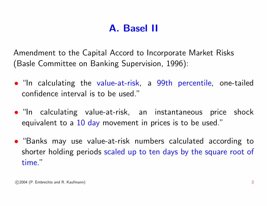
A. Basel II

Amendment to the Capital Accord to Incorporate Market Risks

(Basle Committee on Banking Supervision, 1996):

• “In calculating the value-at-risk, a 99th percentile, one-tailed

confidence interval is to be used.”

• “In calculating value-at-risk, an instantaneous price shock

equivalent to a 10 day movement in prices is to be used.”

• “Banks may use value-at-risk numbers calculated according to

shorter holding periods scaled up to ten days by the square root of

time.”


Basel II (cont.)

• Market risk: 10-day value-at-risk, 99%

Standard: 1-day value-at-risk, 95%

• Insurance: 1-year value-at-risk, 99%

1-year expected shortfall, 99%


Value-at-Risk and Expected Shortfall

• Primary risk measure: Value-at-Risk defined as

VaRp(X) = F−1−X(p) ,

i.e. the pth quantile of F−X. (X denotes the profit, −X the loss.)

• Alternative risk measure: Expected shortfall defined as

ESp(X) = E(−X

∣∣ X < −VaRp

);

i.e. the average loss when VaR is exceeded. Sp(X) gives

information about frequency and size of large losses.


VaR in Visual Terms

Profit & Loss Distribution (P&L)

prob

abilit

y de

nsity

-10 -5 0�

5�

10

0.0

0.05

0.10

0.15

0.20

0.25 Mean profit = 2.495% VaR = 1.6

�

5% probability�


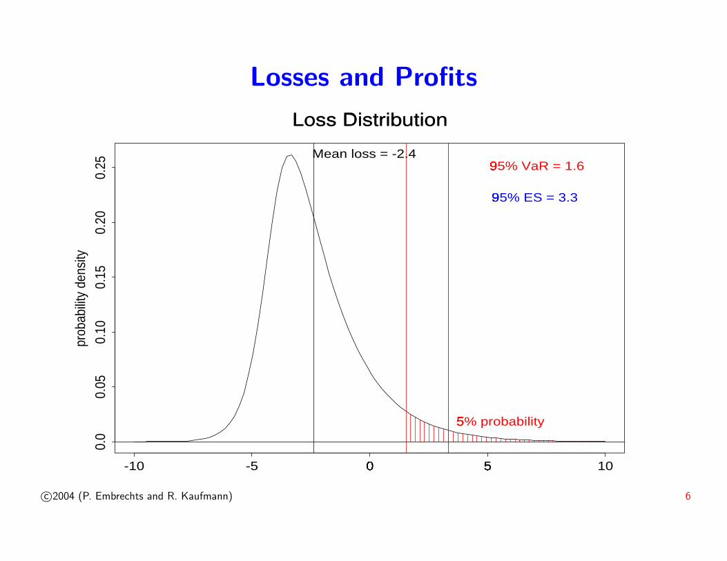
Losses and Profits

Loss Distribution

prob

abilit

y de

nsity

-10 -5 0�

5�

10

0.0

0.05

0.10

0.15

0.20

0.25

Mean loss = -2.495% VaR = 1.6

�

5% probability�

95% ES = 3.3�


B. Scaling

Question 1: How to get a 10-day VaR (or 1-year VaR)?

Solution in the praxis: scale the 1-day VaR by√

10 (or√

250).

Question 2: How good is scaling?

→ Model dependent!


Scaling under Normality

Under the assumption

Xii.i.d.∼ N (0, σ2),

n-day log-returns are normally distributed as well:

n∑i=1

Xi ∼ N (0, nσ2).

For a N (0, σ̃2)-distributed profit X, VaRp(X) = σ̃ xp, where xp

denotes the p-Quantile of a standard normal distribution. Hence

VaR(n) =√

n VaR(1).


Accounting for Trends

When adding a constant trend µ,

Xii.i.d.∼ N (µ, σ2),

n-day log-returns are still normally distributed:

n∑i=1

Xi ∼ N (nµ, nσ2).

Hence

VaR(n) + nµ =√

n (VaR(1) + µ),i.e.

VaR(n) =√

n VaR(1) − (n−√

n)µ.


Autoregressive Models

For an autoregressive model of order 1,

Xt = λXt−1 + εt, εti.i.d.∼ N (0, σ2),

1-day and n-day log-returns are normally distributed:

Xt ∼ N(

0,σ2

1− λ2

)and

n∑i=1

Xi ∼ N(

0,σ2

(1− λ)2

(n− 2λ

1− λn

1− λ2

)).


Scaling for AR(1) Models

For an AR(1) model with normal innovations,

VaR(n)

VaR(1)=

√1 + λ

1− λ

(n− 2λ

1− λn

1− λ2

).

For small values of λ,√

n VaR(1) is a good approximation of VaR(n).


Non-Normal Innovations

Question: Is scaling with√

n still appropriate if innovations are

non-normal?

Example: random walk, Xii.i.d.∼ t8

Based on 250 log-returns, how good is√

10 · V̂aR(1)

99% as an

estimate for the 10-day 99% VaR?

(V̂aR(1)

99% denotes the one-day 99% VaR estimate.)


Non-Normal Innovations (cont.)

0.10 0.12 0.140.04 0.06 0.08

0.02

0.04

0.06

0.08

0.12

0.14

0.10

*

**

*

*** *

***

*

*

*

*

**

*

*

**

**

* *

**

*

*

**

*

*

**

**

*

**

*

**

**

*

** **

**

**

****

*

* ***

***

*

*

*

*

*

**

*

**

**

*

*

**

*

*

*

*

******

* **

*

*

*

*

*

*

**

**

*

**

*

*

**

* *

* *

*

*

*

** * *

*

*

*

*

*

**

*

*

*

**

*

**

**

*

*

*

*

* ***

** ** *

*

**

*

*

** *

*

*

*

*

*

*

*

**

*

*

*

*

***

*

*

**

*

*

**

* *

**

*

*

*

**

**

*

* *

*

**

*

* ***

*

*

*

*

**

**

**

*

*** **

*

*

*

*

*

*

*

* *

**

**** *

*

*

*

*

***

**

* *

*

*

**

**

**

****

* ***

*

* *

*

*

*

*

* *

*

*

** **

**

**

** **

*

* **

* **

*

*

*

**

*

*

*

* *

*

*

*

*

**

*

*

**

* ****

*

***

***

*

***

*

* ****

*

*

*

** *

*

*

**

*

*

*

*

*

**

**

* **

*

**

*

**

**

*

* ***

**

*

*

****

*

*

***

*

*

* *

*

*

* ** **

***

*

**

*

*

* *

**

**

**

*

*

*

**

*

***

*

*

*

*

**

**

*

**

*** * * *

*

*

*

*

**

*

*

* *

**

*

*

**

*

*

*

*

*

*

*

**

*

**

**

*

*

*

****

**

*

*

*** *

*

*

**

*

**

*

**

**

*

*

***

*

*

*

***

*

***** *

**

*

*

*

* *

*

*

*

** *

*

*

**

*

*

*

*

**

***

**

*

**

**

**

*

*

*

**

*

*

***

**

*

**

*

*

*

* *

*

*

*

*

*

*

*

*

*

*

* *

*

**

*

**

*

**

***

**

*

**

*

*

* **

**

*

*

** **

**

*

*

* ***

*

* **

**

*

*

*

*

*

*

**

**

*

**

*

*

*

* *

*

*

*

*

*

**

*

*

*

*

*

*

*

*

*

**

**

*

*

*

*

**

*

*

*

*

*

*

**

*

* ***

*

**** **

*

*

*

*

*

**

*

** *

*

**

*

* **

** *

*

*

*

*

*

*

*

**

*

***

**

*

****

*

**

*

*

*

* **

*

*

**

*

*

*

*

*

*

**

*

**

*

**

*

*

*

*

*

*

**

*

**

*

*

*

**

*

*

*

**

*

*

**

*

* *

*

*

*

**

*

*

*

***

**

**

*

*

* **

*

*

*

**

**

*

***

*

**

*

***

*

*

*

*

**

*

*

*

*

*

**

*

* *

** *

**

*

**

* **

*

*

**

*

**

**

*

* **

*

*

**

*

*

**

*

*

*

***

**

*

*

*

*

*

**

*

**

** *

*

*

*

*

**

*

*

**

*

*

*

*

*

* *

*

* **

*

*

* *

***

*

**

*

**

**

*

*** *

*

*

*

* *

*

*

**

*

** *

**

*

*

*

* *

**

**

*

*

***

*

**

*

*

*

*

**

*

**

*

* *

*

*

**

*

*

*

** *

*

**

* *

**

***

*

**

random walk, t8

sqrt(10) * 1−day−VaR (99%)

10−

day−

VaR

(99

%);

em

piric

al

Scaling is still good, but other methods like random resampling

perform slightly better.


AR(1)-GARCH(1,1) Processes

A more complex process, often used for practical applications, is

the GARCH(1,1) process (λ = 0) and its generalization, the

AR(1)-GARCH(1,1) process:

Xt= λXt−1 + σtεt,

σ2t = a0 + a(Xt−1 − λXt−2)2 + b σ2

t−1,

εt i.i.d., E[εt] = 0, E[ε2t ] = 1.

(typical parameters: λ = 0.04, a0 = 3 · 10−6, a = 0.05, b = 0.92)


● ● ● ●●

●●

●

●

●

●

●

■ ■ ■■ ■ ■

■

■

■

■

■

■

◆ ◆ ◆ ◆◆

◆

◆

◆

◆

◆

◆

◆

0.0 0.05 0.10 0.15 0.20

0.08

0.09

0.10

◆ 10-day, t4 innovations◆ scaled 1-day, t4 innovations■ 10-day, t8 innovations■ scaled 1-day, t8 innovations● 10-day, normal innovations● scaled 1-day, normal innovations

Scaling for AR(1)-GARCH(1,1) Processes

Goodness of fit of the scaling rule, depending on different values of

λ (x axis) for different distributions of the innovations εt.

For typical parameters (λ = 0.04, εt ∼ t8), the fit is almost perfect.


GARCH(1,1) vs. Random Walk

A GARCH(1,1) process

Xa,t = σa,tεt,

σ2a,t = a0 + aX2

a,t−1 + b σ2a,t−1,

εt i.i.d., E[εt] = 0, E[ε2t ] = 1,

(where a is typically close to 0) can be approximated by a process

with variance

σ20,t = a0 + b σ2

0,t−1

or

σ20,t = a0 + (a + b) σ2

0,t−1.


GARCH(1,1) vs. Random Walk (cont.)

If the initial values of the processes (Xa,t) and (X0,t) coincide, then

E[(Xa,t −X0,t)2] ≤ fct(parameters),

and

E[(n+h∑

t=n+1

Xa,t −n+h∑

t=n+1

X0,t)2] ≤ fct(parameters).

These inequalities can be used to get bounds for (conditional and

unconditional) value-at-risk of GARCH(1,1) processes. Analogously,

value-at-risk estimates for AR(1)-GARCH(1,1) processes can be

obtained by approximating them with AR(1) processes.


Stochastic Volatility Model with Jumps

An alternative to autoregressive types of models are stochastic

volatility models:

Xt = a σt Zt + b Jt εt,

σt = σφt−1 ec Yt,

εt, Zt, Yti.i.d.∼ N (0, 1),

Jti.i.d.∼ Bernoulli(λ)

(typical parameters:

λ = 0.01, a = 0.01, b = 0.05, c = 0.05, φ = 0.98)


Stochastic Volatility Model: Volatility and Returns

0 50 100 150 200 250

0.8

1.0

1.2

1.4

1.6

1.8

0 50 100 150 200 250


Scaling in the Stochastic Volatility Model

0.0 0.02 0.04 0.06 0.08 0.10

0.08

0.12

0.16

0.20

10−day VaRscaled 1−day VaR

Goodness of fit of the scaling rule, depending on different values of

λ (x axis).

The scaled 1-day VaR underestimates the 10-day VaR for small

values of λ. For λ > 0.04, this changes to an overestimation.


C. One-Year Risks

Problems when modelling yearly data:

• Non-stationarity of data sets.

• Lack of yearly returns.

• Properties of yearly data are different from those of daily data.


How to Estimate Yearly Risks

• Fix a horizon h < 1 year, for which data can be modelled.

• Use a scaling rule for the gap between h and 1 year.

suitable model

scaling rule

today h days 1 year


Models

• Random Walks

• Autoregressive Processes

• GARCH(1,1) Processes

• Heavy-tailed Distributions


Random Walk

Financial log-data (st)t∈hN can be modelled as a randow walk

process with constant trend and normal innovations:

st = st−h + Xt, Xti.i.d.∼ N (µ, σ2) for t ∈ hN.

The square-root-of-time rule (accounting for the trend) can be used

to scale h-day risks to 1-year risks.


Autoregressive Processes

For an AR(p) model with trend and normal innovations,

st =p∑

i=1

ai st−ih + εt for t ∈ hN,

(εt ∼ N (µ0 + µ1 t, σ2), independent)

the 1-year value-at-risk and expected shortfall can be calculated as a

function of the parameters µ1, σ and ai, and the current and past

values of (st).


Generalized Autoregressive ConditionalHeteroskedastic Processes

Assuming a GARCH(1,1) process with Student-t distributed

innovations for h-day log-returns,

Xt = µ + σt εt for t ∈ hN,

σ2t = α0 + α1(Xt−h − µ)2 + β1σ

2t−h,

where εti.i.d.∼ tν, E[εt] = 0, E[ε2t ] = 1,

1-year log-returns follow a so-called weak GARCH(1,1) process. The

corresponding VaR and ES can be calculated as a function of the

above parameters and the current and past values of (Xt).


Heavy-tailed Distributions

h-day log-returns (Xt)t∈hN are said to have a heavy-tailed

distribution, if

P [Xt < −x] = x−αL(x) as x →∞,

where α ∈ R+ and L is a slowly varying function,

i.e. limx→∞L(sx)L(x) = 1 for all s > 0.

Also in this case, 1-year VaR and ES can be estimated based on the

parameter α and on the observed data.


Backtesting

The suitability of these models for estimating one-year financial risks

can be assessed by comparing estimated value-at-risk and expected

shortfall with observed return data for

• stock indices,

• foreign exchange rates,

• 10-year government bonds,

• single stocks.


Conclusions for 1-Year Forecasts

• The random walk model performs in general better than the other

models under investigation. It provides satisfactory results across

all classes of data and for both confidence levels investigated (95%,

99%). However, like all the other models under investigation, the

risk estimates for single stocks are not as good as those for foreign

exchange rates, stock indices, and 10-year bonds.

• The optimal calibration horizon is about one month. Based on

these data, the square-root-of-time rule (accounting for trends) can

be applied for estimating one-year risks.


Confidence Intervals for a Random Walk

0.1

0.2

0.3

0.4

0.5

0.6

*

*

h = 1 day

*

*

h = 1 week

*

*

h = 1 month

*

*

h = 3 months

*

*

h = 1 year

Point estimates and 95% confidence intervals for one-year

99% expected shortfall and 99% value-at-risk (percentage loss) for a

simulated random walk with normal innovations.


D. Conclusions

• The square-root-of-time scaling rule performs very well to scale

risks from a short horizon (1 day) to a longer one (10 days, 1 year).

• The reasons for this good performance are non-trivial. Each

situation has to be investigated separately. The square-root-of-

time rule should not be applied before checking its appropriateness.

• In the limit, as α → 1, scaling a short-term VaRα to a long-term

risk using the square-root-of-time rule is for most situations not

appropriate any more.


Further Work

• An interesting subject for further research is to find the limits,

where the square-root-of-time rule fails. For example changing

one single parameter in a model can have a strong effect on the

appropriateness of this scaling rule.

• Linked to this topic is the model-dependent question, why the

square-root-of-time rule performs well (or not so well) in a certain

situation.

• An interesting generalisation of this work would be the investigation

of multivariate models.


Bibliography

[Brummelhuis and Kaufmann, 2004a] Brummelhuis, R. and Kauf-

mann, R. (2004a). GARCH(1,1) and AR(1)-GARCH(1,1) pro-

cesses: perturbation estimates for value-at-risk. Working Paper.

[Brummelhuis and Kaufmann, 2004b] Brummelhuis, R. and Kauf-

mann, R. (2004b). Time Scaling for GARCH(1,1) and AR(1)-

GARCH(1,1) Processes. Working Paper.

[Embrechts et al., 2004] Embrechts, P., Kaufmann, R., and Patie,

P. (2004). Strategic long-term financial risks: Single risk factors.

To appear in: A special issue of Computational Optimization and

Applications.


[Kaufmann, 2004a] Kaufmann, R. (2004a). Long-Term Risk Manage-

ment. PhD Thesis, ETH Zurich.

[Kaufmann, 2004b] Kaufmann, R. (2004b). Time Scaling for Sto-

chastic Volatility Models. Working Paper, ETH Zurich.

[Kaufmann and Patie, 2003] Kaufmann, R. and Patie, P. (2003).

Strategic Long-Term Financial Risks: The One Dimensional Case.

RiskLab Report, ETH Zurich. Available at http://www.risklab.ch/

Papers.html#SLTFR.


Modelling of Long-Term Risk - ETH Zembrecht/ftp/LongTermRisk.pdf · Modelling of Long-Term Risk...

Documents

Transcript of Modelling of Long-Term Risk - ETH Zembrecht/ftp/LongTermRisk.pdf · Modelling of Long-Term Risk...