Modelling of Ground Support in Tunneling using the BEM
177
Institut f¨ ur Baustatik – Institute for Structural Analysis Lessingstraße 25/II 8010 Graz, Austria PhD Thesis Modelling of Ground Support in Tunnelling using the BEM by Katharina Riederer submitted on December 20th, 2009 Primary Advisor : Gernot Beer Institute for Structural Analysis Graz University of Technology, Austria Second Examiner : Adri´ an Pablo Cisilino Department of Mechanical Engineering University of Mar del Plata, Buenos Aires, Argentina
Transcript of Modelling of Ground Support in Tunneling using the BEM

Institut fur Baustatik –Institute for Structural Analysis
Lessingstraße 25/II8010 Graz, Austria
PhD Thesis
Modelling of Ground Support
in Tunnelling using the BEM
by
Katharina Riederer
submitted on December 20th, 2009
Primary Advisor : Gernot Beer
Institute for Structural AnalysisGraz University of Technology, Austria
Second Examiner : Adrian Pablo Cisilino
Department of Mechanical EngineeringUniversity of Mar del Plata, Buenos Aires, Argentina


iii
Abstract
Numerical simulation is a growing and important tool in the field of tunnel
construction; it can be very helpful, allowing the investigation of various alter-
natives in virtual reality rather than reality. Selecting the best option can result
in significant cost savings, reduced construction time and in improved safety.
Commonly used methods require a significant amount of computational costs
especially for large 3D simulations. The effort for mesh generation as well as
the calculation time increase considerably.
An attractive alternative for simulating tunnelling problems is the Boundary
Element Method (BEM). In this method the discretised mesh is much smaller
and simpler, thus the mesh generation is more user-friendly, the calculation
time is shorter and the mesh is less error-prone. The effort to do 3D simulations
is significantly reduced. However, the BEM is not as far developed as other
methods at the moment. There are currently no commercial programs available
that include all the features required for conventional tunnelling, for example
the simulation of ground support and ground improvement techniques.
The aim of this work was the development and the implementation of methods
to simulate ground support (rock bolts and pipe roofs) into the BEM pro-
gram (BEFE++). Novel methods were developed to simulate these inclusions
efficiently and realistically.
In these methods the inclusions are simulated by applying stresses or forces to
the system. These stresses or forces are calculated within an iterative algorithm.
Because of this, a huge number of inclusions (for example rock bolts) can be
calculated efficiently and the iterative procedure can be easily combined with

iv
a non-linear calculation (for example to simulate plastic material behaviour).
Next to the simulation of rock bolts and pipe roofs these methods can be used
to simulate geological inhomogeneities as well. In contrast to commonly used
methods the mesh generation for such problems is very easy and independent
from any domain discretisation. This means a considerable increase in user
friendliness and accuracy especially for the simulation of rock bolts in comparison
with other methods. The high stress variations in the near-field of the bolt can
be simulated more accurately. With a relative small effort very accurate results
are obtained.
Keywords: Boundary Element Method, body forces, internal cells, inclu-
sions, inhomogeneities, tunnelling, ground support, rock bolts, anchors, pipe
umbrella.

v
Kurzfassung
Um Tunnelbauprojekte hinsichtlich Sicherheit, Kosten und Qualitat zu op-
timieren werden realitatsnahe numerische Simulationen sowohl in der Pla-
nungsphase als auch wahrend der Ausfuhrung eingesetzt. Derzeit verwendete
Simulationsmethoden stoßen speziell bei der Berechnung von großen 3D Problem-
stellungen schnell an ihre Grenzen. Der Rechen- und Modellierungs- Aufwand
steigt enorm an.
Eine attraktive Alternative dazu stellt die Randelemente Methode (REM)
dar. Durch ein kleineres, einfaches und uberschaubares Netz wird die Netz-
generierung benutzerfreundlicher, die Berechung weniger Fehleranfallig und der
Rechenaufwand geringer als bei anderen Methoden. Das stellt speziell bei 3D
Simulationen einen wesentlichen Vorteil dar. Allerdings ist die REM noch nicht
auf dem gleichen Entwicklungsstand wie derzeit gangige Methoden. Es sind bis
heute noch keine kommerziellen Randelemente Programme erhaltlich die in der
Lage sind alle notigen Bestandteile eines konventionellen Tunnelvortriebs zu
simulieren (wie z.B. den Einbau verschiedener Stutzmittel usw.).
Ziel dieser Arbeit war die Entwicklung von Methoden zur Simulation von
Stutzmitteln (Felsanker und Rohrschirme) in das Randelemente Programm
(BEFE++) und deren Implementierung . Es wurden vollig neue Methoden
entwickelt um diese Einschlusse effizient und realitatsnah zu simulieren. Dabei
werden anstelle der Einschlusse Spannungen oder Krafte auf das System aufge-
bracht welche diese Einschlusse simulieren. Diese Spannungen oder Krafte
werden mithilfe eines iterativen Algorithmus berechnet. Durch dieses iterative
Verfahren kann eine große Anzahl von Einschlussen (Felsankern, Rohrschirme)
effizient berechnet werden und der Algorithmus kann einfach und effektiv mit

vi
einer nichtlinearen Berechnung (z.B. bei plastischem Materialverhalten) kom-
biniert werden. Neben der Berechnung von Felsankern und Rohrschirmen
kann diese Methode auch zur Simulation von geologischen Inhomogenitaten
herangezogen werden. Die Generierung eines solchen Netzes ist denkbar ein-
fach und unabhanging von einer Bereichs-diskretisierung. Dies stellt besonders
bei der Simulation von Felsankern eine wesentliche Verbesserung gegenuber
derzeit verwendeten Methoden dar. Die hohen Spannungsvariationen im Umfeld
des Ankers konnen sehr genau wieder gegeben werden. Mit relativ geringem
Rechenaufwand werden qualitativ hochwertige Ergebnisse erzielt.
Schlusselworter: Rand Elemente Methode, Volumskrafte, Zellen, Einschlusse,
Inhomogenitaten, Tunnel, Stutzmittel, Felsanker, Rohrschirm.

vii
Contents
1 Introduction 11.1 Motivation . . . . . . . . . . . . . . . . . . . . . . . . . . . . . . 11.2 Conventional Tunnelling . . . . . . . . . . . . . . . . . . . . . . 4
1.2.1 Historical Development . . . . . . . . . . . . . . . . . . . 41.2.2 Design Philosophy and Construction Method . . . . . . . 7
1.3 Computational Modelling . . . . . . . . . . . . . . . . . . . . . 101.4 Structure of this work . . . . . . . . . . . . . . . . . . . . . . . 19
2 Boundary Element Method 212.1 Introduction . . . . . . . . . . . . . . . . . . . . . . . . . . . . . 21
2.1.1 Numerical Simulation of Engineering Problems . . . . . . 212.2 Physical Model . . . . . . . . . . . . . . . . . . . . . . . . . . . 222.3 Integral Formulation . . . . . . . . . . . . . . . . . . . . . . . . 24
2.3.1 Betti’s Theorem . . . . . . . . . . . . . . . . . . . . . . . 252.3.2 Somigliana’s Identity . . . . . . . . . . . . . . . . . . . . 272.3.3 Fundamental Solutions . . . . . . . . . . . . . . . . . . . 292.3.4 Boundary Integral Equation . . . . . . . . . . . . . . . . 312.3.5 Body Forces . . . . . . . . . . . . . . . . . . . . . . . . . 352.3.6 Internal Results . . . . . . . . . . . . . . . . . . . . . . . 39
2.4 Numerical Implementation . . . . . . . . . . . . . . . . . . . . . 462.4.1 Discretisation of the Boundary Geometry . . . . . . . . . 462.4.2 Approximation of Physical Quantities . . . . . . . . . . . 492.4.3 Discretisation inside the Domain . . . . . . . . . . . . . 502.4.4 Matrix Assembly / System of equations . . . . . . . . . . 522.4.5 Numerical Integration . . . . . . . . . . . . . . . . . . . 54
2.5 Singular Integrals . . . . . . . . . . . . . . . . . . . . . . . . . . 612.5.1 Weak Singularity . . . . . . . . . . . . . . . . . . . . . . 612.5.2 Strong Singularity . . . . . . . . . . . . . . . . . . . . . 62
2.6 Conclusion . . . . . . . . . . . . . . . . . . . . . . . . . . . . . . 63
3 Solution Procedure for Embedded Inclusions 653.1 Introduction . . . . . . . . . . . . . . . . . . . . . . . . . . . . . 65

viii Contents
3.2 Body Force Approach . . . . . . . . . . . . . . . . . . . . . . . . 673.2.1 Direct Solution Procedure . . . . . . . . . . . . . . . . . 693.2.2 Iterative Solution Procedure . . . . . . . . . . . . . . . . 71
3.3 Conclusion . . . . . . . . . . . . . . . . . . . . . . . . . . . . . . 77
4 General Inhomogeneities and Pipe Umbrellas 794.1 General . . . . . . . . . . . . . . . . . . . . . . . . . . . . . . . 79
4.1.1 General Inhomogeneities . . . . . . . . . . . . . . . . . . 794.1.2 Pipe Umbrellas . . . . . . . . . . . . . . . . . . . . . . . 80
4.2 BE-approach . . . . . . . . . . . . . . . . . . . . . . . . . . . . 824.2.1 Iterative Procedure . . . . . . . . . . . . . . . . . . . . . 824.2.2 Computation of the Strains . . . . . . . . . . . . . . . . 834.2.3 Computation of the Residuum . . . . . . . . . . . . . . . 854.2.4 Evaluation of the Integral . . . . . . . . . . . . . . . . . 88
4.3 Verification Examples . . . . . . . . . . . . . . . . . . . . . . . . 894.3.1 Example 1: Soft inclusion in plane strain . . . . . . . . 894.3.2 Example 2: Soft inclusion in 3D . . . . . . . . . . . . . 914.3.3 Example 3: Soft inclusion and multiple regions . . . . . 934.3.4 Example 4: Cantilever with stiff inclusion in second
analysis step . . . . . . . . . . . . . . . . . . . . . . . . 94
5 Continuous Anchored Bolts 975.1 General . . . . . . . . . . . . . . . . . . . . . . . . . . . . . . . 975.2 BE-approach . . . . . . . . . . . . . . . . . . . . . . . . . . . . 100
5.2.1 Iterative Procedure . . . . . . . . . . . . . . . . . . . . . 1005.2.2 Line-cells . . . . . . . . . . . . . . . . . . . . . . . . . . 1015.2.3 Computation of Stresses in Axial Bolt Direction . . . . . 1025.2.4 Computation of the Residuum . . . . . . . . . . . . . . . 1065.2.5 Evaluation of the Integral . . . . . . . . . . . . . . . . . 111
5.3 Verification Examples . . . . . . . . . . . . . . . . . . . . . . . . 1205.3.1 Example 1: Fully grouted rock bolt in plane strain . . . 1205.3.2 Example 2: Fully grouted rock bolt in 3D . . . . . . . . 1215.3.3 Example 3: Bond Slip Effects . . . . . . . . . . . . . . . 1215.3.4 Example 4: Yielding Bolt . . . . . . . . . . . . . . . . . 122
6 Discrete Anchored Bolts 1256.1 General . . . . . . . . . . . . . . . . . . . . . . . . . . . . . . . 1256.2 BE-approach . . . . . . . . . . . . . . . . . . . . . . . . . . . . 127
6.2.1 Iterative Procedure . . . . . . . . . . . . . . . . . . . . . 1276.2.2 Pair of Points . . . . . . . . . . . . . . . . . . . . . . . . 1286.2.3 Computation of Bolt Strains and Bolt Forces . . . . . . . 130

Contents ix
6.2.4 Computation of the Residuum . . . . . . . . . . . . . . . 1316.2.5 Evaluation of the body force terms . . . . . . . . . . . . 134
6.3 Verification Examples . . . . . . . . . . . . . . . . . . . . . . . . 1396.3.1 Example 1: Discrete anchored bolt in plane strain (with
pre-stressing) . . . . . . . . . . . . . . . . . . . . . . . . 1396.3.2 Example 2: Discrete anchored bolt in 3D . . . . . . . . . 140
7 Examples 1417.1 Plane Strain Examples . . . . . . . . . . . . . . . . . . . . . . . 141
7.1.1 Example 1: Tunnel with plasticity and rock bolts . . . . 1417.1.2 Example 2: Tunnel with inclusion and rock bolts . . . . 1437.1.3 Example 3: Tunnel with plasticity, rock bolts and pipe roof146
7.2 Three Dimensional Example . . . . . . . . . . . . . . . . . . . . 1487.2.1 Tunnel with plasticity, rock bolts and pipe roof . . . . . 148
8 Conclusions 155
Bibliography 157
List of Figures 163
List of Tables 167

x

1
Chapter 1
Introduction
1.1 Motivation
In the design of engineering structures, numerical simulation plays an increasingly
important role. This has become very popular due to rapid advancements in
computer technology and its availability to engineers. Numerical techniques
have been developed for solving many kinds of engineering problems, also in
the field of underground engineering structures.
For tunnelling problems, numerical techniques help the designer in dimensioning
the opening, selecting the best alignment, the best excavation sequence, choosing
and dimensioning the support structures, and to quantitatively assess its overall
behaviour through parametric or sensitivity studies. Diverse information about
geology, physics, construction techniques, economy, the environment and their
interactions can be considered. Problems with arbitrary shape, with nonlinear
material behaviour, consideration of ground support, self weight, external forces,
in situ stresses, pre-stressing, etc. can be calculated. All this achievements
have greatly enhanced the development of modern rock mechanics; see Jing and
Hudson (2002), Gioda and Swoboda (1999), Pande et al. (1990). Simulations
allow testing of various alternatives in virtual reality rather than reality; this
results in significant cost savings, reduction of construction time and makes
tunnelling safer.
2 1. Introduction
A number of computational methods have been developed. However, it is
clear that a very important step in numerical simulation is the early choice
of the best numerical method in terms of scope, accuracy, efficiency and user-
friendliness. The Finite Element Method (FEM) is perhaps the most widely
applied numerical method in engineering fields. Today’s FEM-programs have
reached a very high development-stage; almost all important features involved
in underground engineering problems are included. However, it has some
disadvantages as well:
Domain based methods, like the FEM are techniques in which the discretisation
has to be introduced in the entire domain. In tunnelling this means the
discretisation of the whole surrounding rock mass into small elements. Thus,
one can imagine that the system of equations and the effort for mesh generation
become very huge; especially for three dimensional analyses. The required
effort is the reason why unrealistic 2-D analyses are often carried out instead.
However, the advancing process of a tunnel has an essentially 3D nature. 3D
modelling is necessary for the simulation of effects ahead of the tunnel face,
of the correct stress-strain distribution, the non-linear behaviour of the rock
mass, and the influence of support measures. Furthermore, when simulating
tunnels supported by rock bolts, the mesh around the bolts has to be extremely
fine to handle the local stress concentrations. This problem leads either to an
extremely large number of elements or to inaccurate results.
This leads to the statement that currently used numerical methods have major
drawbacks with respect to user-friendliness and efficiency. An attractive alterna-
tive is the Boundary Element Method (BEM), where only the excavation surface
has to be discretised and the effort to do 3D simulations is significantly reduced.
However, the BEM is much less developed than the FEM and currently there are
no commercial programs available that are able to include all relevant features
for tunnelling problems in their calculation. This means especially the following
features: calculation of sequential excavation, non-linear material behaviour,
inhomogeneous ground conditions, support measurements (as shotcrete, rock
bolts or pipe umbrella systems) and a user-friendly pre-processor.

1.1. Motivation 3
The goal of the research activities of the Institute for Structural Analysis at
the University of Technology in Graz is the development of the BE-program
BEFE++ which is especially capable to simulate conventional tunnelling pro-
cesses, including all important features, mentioned before. The calculation of
sequential excavation processes was developed in Duenser (2001); non-linear
material behaviour are discussed by Ribeiro (2006), Thoeni (2009), Prazeres
(2009); and the simulation of shotcrete refer to Prazeres (2009).
This thesis deals with the efficient calculation of rock bolts, pipe umbrella
systems and general inclusions such as geological inhomogeneities. They have
one thing in common: they are all inclusions inside the domain. Rock bolts are
very narrow inclusions, a pipe umbrella system and geological inhomogeneities
are inclusions with general shape. A novel method was developed that allows to
model rock bolts (and also anchors and geological inclusions) efficiently with the
BEM. An iterative solution procedure is used for solving the problem. Because
of this, the system of equations stays small, even with a very large number
of rock bolts (or anchors or inclusions) and the algorithm can be efficiently
combined with the iterative procedure for the non-linear material behaviour.
Especially for large scale problems, for problems containing a lot of rock bolts
and for problems considering non-linear material behaviour this method is of
great advantage.
The new method is applicable to:
• Passive (or non-stressed) fully grouted rock bolts. Features are included
to calculate bolt yielding and bond slip effects.
• Anchors or bolts which are bonded at the ends (by cement grout, resin,
or fixed by a mechanical anchor) and have a free length in between. They
can be passive or active (pre-stressed) and bolt yielding can be considered.
• Geological inhomogeneities with general shape (which can have non-linear
material behaviour).
• The simulation of pipe roofs (to improve the rock mass behaviour and
stabilise the excavated area). They are approximately simulated by a
homogenized plane-shaped umbrella-zone.

4 1. Introduction
Next the conventional tunnelling will be described briefly and then an intro-
duction to computational modelling will be presented. At the end of this
introductory chapter the structure for the next chapters of this work will be
given.
1.2 Conventional Tunnelling
1.2.1 Historical Development
The history in tunnel engineering is referred in several works, for example Kovari
(2003a,b), Romana (2009), Schubert (1997), Karakus and Fowell (2004). Below
a short overview of the main developments are summarised:
Kovari (2003a) claims that the beginning of tunnel engineering was seen in the
1.1 km long Tronquoy Tunnel in France, built by Napoleon in 1803. Here, for the
first time, a large area of excavation in difficult ground conditions was realised.
Thus, this tunnel is regarded as the first to be built on engineering principles.
Since that, up to the middle of the 19th century, the most important modes
of “ground response” were defined and classified. One of the first publications
on tunnelling was written in 1844, by the Englishman F.W. Simms, see Kovari
(2003a). He already expressed the idea that in the case of deep tunnels “a small
portion only gets into motion, the upper part acting as a key, by which the
mass supports itself”. He clearly states that “it is the mass in adjusting itself to
equilibrium”. An other early and important work on tunnelling was written in
1870 by Rziha (see Schubert (1997)).
Timberwork
At this early state tunnels were supported by timberwork, however this timbering
had a lot of disadvantages (for example: timber structure involved up to 60
percent of the cross-section; over-excavation was necessary; difficult construction
...). The replacement of timbering was introduced gradually, by steel supports,
1.2. Conventional Tunnelling 5
then shotcrete, followed by rock anchors and finally, the systematic combination
of these support measured on a broad scale (at about 1950).
Steel Support
Steel support were used in mining since 1862 (see Kovari (2003a)). At a very early
state (in 1872) also Rziha proposed to replace timberwork by steel supports
(Schubert (1997)). By the end of the 19th century, the basic construction
problems using steel supports had been solved and this support system began
to replace timbering mainly in the United States. In European tunnels, steel
supports were not economical at this time, because of the high material costs in
comparison to the personnel costs; this relation was different than in the United
States.
Shotcrete and Rock bolts
The development of shotcrete and rock anchors represents one of the greatest
advancements in tunnelling history. The first use of these support elements
began already very early in the field of mining, with the first use of rock anchors
in 1913 and that of shotcrete in 1914(Kovari (2003a)).
The development of shotcrete technology started with the American taxidermist
C.E. Akeley; he invented the “cement-gun”. The patent for an “apparatus for
mixing and applying plastic or adhesive materials”, which was called a “cement
gun” was obtained in 1911. During the 1910s, shotcrete was used in mines in
the United States and in the early 1920s it came to Europe. The possibilities
for the application of shotcrete were recognised and utilised very rapidly by the
technical world (see Kovari (2003a), Karakus and Fowell (2004)).
The history of rock bolting began in 1913, with the submission of a patent
by Stephan, Frohlich and Klupfel: “... boreholes of sufficient depth will be
drilled into the rock in which rods, tubes or cables of a load-bearing material,
for example steel, will be inserted and fixed at the end in a proper manner or

6 1. Introduction
cemented along the whole length.” The first World War delayed the issuing of
the patent until 1918, see Kovari (2003b).
Sprayed concrete lining method / New Austrian Tunnelling Method
The combined use of rock bolting, reinforcing nets and sprayed concrete has
been practice in mining in Ontario, Canada, since approximately 1930. Keeley
published 1934 in Canada a work, describing a support concept for mining
which involves the use of expansion-bolts together with sprayed concrete. The
introduction of a shotcreting machine by the Swiss engineer G. Senn in 1950
marks a new area for the sprayed concrete lining method. Since that the sprayed
concrete lining took on a greater role than had earlier been assumed, see Kovari
(2003b).
From about this point the opinions drift apart and the polemic in the interna-
tional tunnelling community is big. One party promotes the idea of the New
Austrian Tunnelling Method as a self-contained new method developed by the
Austrian Rabcewicz. The other party appeal against this Austrian claim and
proposes the name Sprayed Concrete Lining Method.
• One view is that after the introduction of the shotcreting machine 1950,
very soon it was realized all over the world that a combination of shotcrete
and rock anchors in many cases provides the most efficient method (both
structurally and economically). The new methods of support opened sev-
eral novel excavation concepts; and they were summarised as the Sprayed
Concrete Lining Method; in the 1960s this method was firmly estab-
lished. Not until 1963 the Austrian engineer Rabcewicz renamed the
method in “New Austrian Tunnelling Method” (NATM); however, in this
point of view NATM is only a nickname for the sprayed concrete lining
method, which was developed and practised in the international commu-
nity much earlier. For more detailed information see Kovari (2003b).
• The other view is that Rabcewicz had the first ideas for a new method after
his experience in the second World War, building underground bunkers

1.2. Conventional Tunnelling 7
in the Russian front. He invented dual-lining supports (initial and final
support) expressing the concept of allowing the rock to deform before
the application of the final lining so that the loads on lining are reduced.
In 1948 Rabcewicz submitted an Austrian patent about this method.
1956-1958 he risks the first time the application of shotcrete and anchors
as stand-alone support system without other supports for the construction
of the highway- and railway-tunnels in Caracas, Venezuela. 1962 he
proposed the term New Austrian Tunnelling Method (NATM) for
this concept. The first urban application in soft ground of the NATM was
the subway tunnel in Frankfurt, Germany in 1969 by Muller. Detailed
information about the developments of the NATM can be seen in Schubert
(1997), Karakus and Fowell (2004), Romana (2009).
The conflict about the name NATM lead back to the question: Is the NATM a
construction method or is it more than that is it a design philosophy?
1.2.2 Design Philosophy and Construction Method
Rabcewic explains the NATM in 1964 by emphasizing three key points: the first
is the application of a thin-sprayed concrete lining, the second is closure of the
ring as soon as possible and the third is systematic deformation measurement.
However, this definition might not been able to explain neither what’s new
nor what’s Austrian about this method and thus induced the above mentioned
conflicts. Because of that a lot of new definitions evolved which tried to specify
the NATM in more detail; they argue that NATM is a design philosophy rather
than a construction method (a set of excavation and support techniques), see
Karakus and Fowell (2004).
Design Philosophy
Muller, one of the advocators of NATM proposed 1978 that: “The NATM is,
rather, a tunnelling concept with a set of principles... Thus in the autor’s

8 1. Introduction
opinion it should not even called a construction method, since this implies a
method of driving a tunnel.” He summarised the NATM by the following points
(see Romana 2009, Karakus and Fowell 2004): use the rock mass for the support
of the terrain charges; allow deformation in order to develop the rock mass
strength around the tunnel and to minimize the support needs; deformations
must be controlled; design is done during the excavation; basic instrumentation
control is done by convergence measurements.
An other definition was given by the Austrian National Committee on Un-
derground Construction of the International Tunnelling Association (ITA) in
1980, see Karakus and Fowell (2004): “The New Austrian Tunnelling Method
(NATM) is based on a concept whereby the ground (rock or soil) surrounding
an underground opening becomes a load bearing structural component through
activation of a ring like body of supporting ground”.
A more actual definition of the design philosophy NATM has been formulated
by Brown in 1995 (see Romana 2009): “The terrain strength around the tunnel
is mobilized to a maximum possible level; this is done allowing for a controlled
deformation. The primary support is installed with strength-deformation char-
acteristics adequate for the terrain and in a compatible time with the terrain
deformability. Instrumentation is used to control the support deformation
in order to change (if/when necessary) the initial design and the excavation
sequence. Movements at surface and around the tunnel are controlled in urban
environment.“
Construction Method
However, the NATM or Sprayed Concrete Lining Method can also be seen as
a construction method. In 2002 Romero pointed out: ”Tunnel excavation and
support are done in a sequential way. The sequence can be changed. Initial
support by: shotcrete; bolts; steel sets. Secondary lining is (very often, but
not always) concrete put in place with forms.“ Thus, NATM is being used as a
construction method and the design philosophy is not necessarily applied, see
Romana (2009). In soils for example, the deformations are bigger and more
1.2. Conventional Tunnelling 9
difficult to control. In this case it is easy to apply NATM as a construction
method; however, it is difficult to apply NATM as a design philosophy.
As described in Galler (2009) the basic principles of the construction method
NATM can be summarised as the following: Typical support elements in NATM
are shotcrete and rock anchors to allow controllable deformation of the rock
mass. Steel ribs or lattice girders provide limited early support before the
shotcrete hardens and ensure correct profile geometry. Face bolts, sealing
shotcrete and pipe roofs are installed, if ground conditions require support at
or ahead of the excavation face. The subdivision of the excavation cross-section
in top heading, bench and invert depends on geological conditions as well as on
logistical requirements to facilitate the use of standard plant and machinery in
tunnelling. Side drift galleries are provided to limit the size of large excavation
faces and the associated surface settlements.
Different procedures have to be chosen for different ground conditions, see Galler
(2009).
Hard Rock Conditions
In deep rock tunnels, the shotcrete lining thickness does not has to be larger; the
main support elements are long rock anchors (2.5m to 9m length). The shotcrete
lining is slotted and yielding supports are installed to allow deformations without
damaging the shotcrete. Once the stabilisation of the system is confirmed by
monitoring, the slots in the lining are closed with shotcrete. The typical
cross-section for a deep rock tunnel is horse-shoe shaped. The cross-section
is typically subdivided into the top heading (the top half of the tunnel cross
section); the bench (excavated a few hundred meters behind); and an invert
arch (which is only installed if ring closure is required by poor rock conditions).
A ramp between top heading and bench is maintained on one half side of the
cross-section.

10 1. Introduction
Soft Rock Conditions
Shallow tunnels in soft ground situated in an urban environment require a rigid
support. The shotcrete lining is more rigid, the advance length is short, and
a rapid closure as well as a subdivision of the cross-section in side and centre
drifts is necessary. The typical cross-section is similar to the cross-section of
a hard rock tunnel; however an invert arch is arranged in the standard case
throughout. A temporary invert in the top heading is employed in some cases.
Furthermore, elephant feet and the arrangement of a pipe canopy can become
necessary. Face reinforcement with dowels and a supporting core is usually
required. The secondary lining is reinforced and its thickness is adjusted to the
substantial ground loads depending on the depth of overburden.
1.3 Computational Modelling
Since about the 60’s of the last century, a number of computational methods
have been developed for numerical simulation. They have become popular
due to rapid advancements in computer technology and its availability to
engineers. Before, rock structures were designed mainly based on rules of thumb,
experience and a trial and error procedure. Analytical or “closed form” solutions
are available for some simple situations, see Pande et al. (1990). However,
in most cases they simplify the real problem drastically concerning material,
geometry, supports...; see for example Feder and Arwanitakis (1976), Kovari
(2003a), Schweiger (2008), Schubert (1997).
However, the excavation and construction process and the technological details
have a strong influence on the stress/strain distribution in the rock mass and
in its support system. The stress/strain distribution is strongly dependent
of the excavation sequence when dealing with supported openings or with
non-linear material behaviour. Another important aspect is the complex geo-
metrical nature; this is not only related to the shape of the opening, but also to
discontinuities in the rock mass, of non-homogeneous or non-isotropic layers,

1.3. Computational Modelling 11
etc. This represents the main drawback for the analytical solutions, or for the
approximated “standard” methods, which in most cases cannot consider this
aspects with sufficient approximation, see Gioda and Swoboda (1999).
Today a number of advanced numerical techniques exist which are able to
simulated underground engineering problems very accurately. Numerical tech-
niques can help the designer in dimensioning the opening, in determining the
loads carried by support structures and for quantitatively assessing its overall
behaviour through parametric or sensitivity studies, see Gioda and Swoboda
(1999). It is possible to analyse problems with arbitrary shape, nonlinear mate-
rial behaviour, considering ground support, self weight, external forces, in situ
stresses, pre-stressing, etc, see Pande et al. (1990).
A categorisation into four principal modelling methods can be pointed out (see
Jing and Hudson 2002):
• Design based on previous experience:
pre-existing standard methods; precedent type analyses
• Design based on simplified models:
analytical methods; rock mass classification
• Design based on numerical modelling which attempts to capture most
relevant mechanisms:
basic numerical methods (FEM, BEM, FDM, DEM)
• Design based on “all-encompassing modelling”:
extended numerical methods; integrated systems approaches
Indeed, computing techniques have become daily tools for formulating diverse
information about geology, physics, construction techniques, economy, the
environment and their interactions. This achievement has greatly enhanced the
development of modern rock mechanics - from the traditional “empirical” art of
rock deformability, strength estimation and support design; to the rationalism
of modern mechanics, see Jing and Hudson (2002).
Whereas the most commonly applied numerical methods for rock mechanics
problems are (see Jing and Hudson 2002):

12 1. Introduction
• Continuum methods
– Finite Element Method (FEM)
– Finite Difference Method (FDM)
– Boundary Element Method (BEM)
• Discrete methods
– Discrete Element Method (DEM)
– Discrete Fracture Network (DFN)
• Hybrid continuum/discrete methods
Special issues and difficulties in numerical modelling of underground engineering
problems are (see Jing and Hudson 2002):
• Scale effects, homogenization and upscaling methods
• Numerical representation of engineering processes, such as excavation
sequence, grouting and reinforcement
• Large-scale computational capacities
• Representation of rock mass properties and behaviour as an equivalent
continuum
• Quantification of fracture shape, size ...
It is clear that a very important step in numerical simulation is the early
“conceptualisation” of the problem in terms of the dominant processes and their
mathematical presentation. Thus, the choice of the best numerical method
in terms of scope, accuracy, efficiency and user-friendliness is very important.
Below the mostly used numerical methods are described briefly to have a better
comparison later on.
Finite Element Method
The FEM is perhaps the most widely applied numerical method in engineering
fields. Since its origin in the early 1960s, much work has been done in both
theoretical developments and applications, and it has been applied to a large

1.3. Computational Modelling 13
number of problems in widely different fields. Today’s FE-programs have
reached such a stage that almost all important features involved in underground
engineering problems are solved. This has been because it was the first numerical
method with enough flexibility for the treatment of material heterogeneity, non-
linear deformability, complex boundary conditions, in situ stresses and gravity,
see Jing and Hudson (2002), Venturini (1983).
The physical meaning of the calculation-steps is relatively transparent: The
method essentially involves dividing the body in smaller “elements” of various
shapes, connected at the nodes. The displacements at the nodes are treated as
unknowns and are calculated, see Pande et al. (1990).
The advantages and disadvantages of the FEM can be summarised (see Schweiger
2008, Venturini 1983, Pande et al. 1990):
Advantages:
• almost no limitations with respect to modelling complex geometries;
• construction steps; advanced constitutive models; change material proper-
ties during calculation;
• special elements for modelling joint sets;
• interface elements for soil/structure interaction; extensively used -> sig-
nificant experience available;
• system of equations is normally banded and symmetric for constitutive
models with associated flow rule;
• each element can have different material properties.
Disadvantages:
• volume discretisation required (significant pre- and postprocessing effort
for 3D analysis);
• long calculation times for 3D and high disk storage requirements;
• non-symmetric equation system for constitutive models with non-associated
flow rule;

14 1. Introduction
• modelling of post peak behaviour (softening material) requires special
formulations and algorithms;
• not suitable for blocky structures (discontinua).
However, for simulating problems like narrow fractures or reinforcements inside
large scale problems the FEM is handicapped by the requirement of very
small element sizes in the nearfield of the narrow discontinuity. This overall
shortcoming makes the FEM less efficient in dealing with fracture problems
than its BEM counterparts, see Jing and Hudson (2002).
Boundary Element Method
This method consists of transforming the governing partial differential equation
into an integral equation relating only boundary values. As a direct consequence,
the dimension of the problem is reduced by one. Only the surface (the boundary)
of the rock mass to be analysed needs to be discretised, i.e. divided into boundary
elements. The domain does not need to be discretised, thus the data preparation
is relatively simple. Smaller systems of equations are obtained as compared
with those from domain type techniques (e.g. FEM or DEM), see Venturini
(1983), Pande et al. (1990).
In the BEM a lot of development work has been done; but the BEM has
not yet reached the development-stage as the FEM. However, applications for
general stress and deformation analysis for underground excavations, fracturing
processes, dynamic analysis, soil-structure interaction and groundwater flow
have been developed. The BEM can range from simple techniques such as the
so-called indirect methods to the more versatile direct formulation, see Venturini
(1983).
Inclusion of source terms, such as body forces, heat sources etc. leads to domain
integrals in the BEM. This problem also appears when considering initial
stress/strain effects for example for non-linear material behaviour. Different
techniques have been developed over the years for dealing with such domain

1.3. Computational Modelling 15
integrals; one of them is the division of the domain into a number of internal
cells, see Jing and Hudson (2002).
In the field of rock mechanics, the most notable original development of the
BEM application may be attributed to early works, see for example: Venturini
(1983), Brebbia et al. (1984), Pande et al. (1990), for a more detailed literature
review see Jing and Hudson (2002), Jing (2003), Gioda and Swoboda (1999).
BEM appears to be a very efficient method for homogeneous, linear elastic
problems, particularly in three dimensions. For complex nonlinear material laws
with a number of sets of materials, advantages of the method are considerable
diminished. The matrices of equations arising in this method are not banded
and symmetric as for FEM, but are fully populated. Thus, although the number
of equations to be solved is considerably reduced, computation time does not
reduce in the same proportion, see Pande et al. (1990).
A great enhancement in comparison to the FEM is the BEMs applicability
for stress or strain analysis problems. The solutions inside the domain are
continuous; stress and strain results inside the domain have the same accuracy
as displacement results. However the BEM is not as efficient as the FEM
in dealing with material heterogeneities. The BEM is also not as efficient as
the FEM in simulating non-linear material behaviour, such as plasticity and
damage evolution processes. The BEM is more suitable for solving problems
of fracturing in homogeneous and linearly elastic bodies, see Jing and Hudson
(2002).
The advantages and disadvantages of the BEM can be summarised (see Schweiger
2008, Venturini 1983):
Advantages:
• only surface discretisation, no volume discretisation required;
• reduced set of equations, smaller amount of data;
• no interpolation error inside the domain;
• better accuracy of stress/strain results;

16 1. Introduction
• proper modelling of infinite domains;
• valuable representation for stress concentration problems.
Disadvantages:
• equation system is non-symmetric and fully populated;
• not well suited to nonlinear material behaviour;
• not well suited to inhomogeneous material;
• modelling of excavation sequence is more difficult.
Finite Difference Method
The Finite Difference Method (FDM) was the first numerical approach formu-
lated on mathematical bases which has been applied in continuum mechanics
stress analysis. The method started as a numerical technique after Southwell had
presented his relaxation method (1946), although no computer automatisation
was possible at that time, see Venturini (1983).
In the FDM the partial differential equations (PDE) are approximated by
replacing the derivative expressions by linear combinations of function values at
the neighbouring grid points. With this the PDE is replaced by a linear system
using only nodal values. With proper formulations, such as static or dynamic
relaxation techniques, no global system of equations in matrix form needs to be
solved. It also provides a more straightforward simulation of nonlinear material
behaviour, such as plasticity and damage. The conventional FDM with regular
grid system is not flexible in dealing with complex boundary conditions, material
heterogeneities and fractures. However, progress has been made with irregular
meshes, such as triangular grid or Voronoi grid systems, which leads to Finite
Volume techniques (FVM), see Jing and Hudson (2002).
One very attractive feature of FDM is that it can be very easy implemented.
The quality of a FEM approximation is often higher than in the corresponding
FDM approach, but this is extremely problem dependent, see Wikipedia.

1.3. Computational Modelling 17
The advantages and disadvantages of the FDM can be summarised by (see
Schweiger 2008):
Advantages:
• complex constitutive models easier to implement;
• no equation system is required for explicit solution algorithms.
Disadvantages:
• volume discretisation required;
• slightly less versatile with respect to geometric discretisation;
• not the same range of higher order elements available;
• long calculation times in 3D;
• for linear or moderately nonlinear systems less efficient than FEM;
• method is based on Newton’s law of motion thus no “converged” solution
for static problems exist (artificial damping required; long calculation
time; with different time steps it converges to different solutions).
Discrete Element Method
In this method the rock mass is treated as a discontinuum. The domain is
assumed to consists of rigid or deformable blocks/particles and the contacts
between them need to be identified and updated during the deformation/motion
process. When loads are applied, the changes in contact forces are traced with
time. In the earlier versions of the method rigid spherical balls or discs were
used as elements. In the recent versions of the method, the elements can be of
arbitrary shape and they can be deformable. The elements can split up based
on the assumed fracture criterion, see Pande et al. (1990), Jing and Hudson
(2002).
This method is based on the equation of motion using implicit and explicit
formulations. The implicit DEM is represented mainly by the discontinuous
deformation analysis (DDA) approach. It uses standard FEM meshes over

18 1. Introduction
blocks and the contacts are treated using the penalty method. The implicit
DDA has two advantages over the explicit DEM: larger time steps and closed-
form integrations for the stiffness matrices of elements, see Jing and Hudson
(2002). The DEM is one of the most rapidly developing areas of computational
mechanics, and it has wide applications in rock engineering.
There are, however, several drawbacks. Firstly, the parameters required for the
description of the material behaviour and additional parameters like damping
are required to be chosen quite carefully. And the computation time required
to solve even simple problems can be excessive, see Pande et al. (1990).
The advantages and disadvantages of the DEM can be summarised by (see
Schweiger 2008):
Advantages:
• modelling of blocky structures (discontinua);
• for explicit solution algorithms no equation system required;
• suitable for studying micromechanical behaviour of granular materials.
Disadvantages:
• volume discretisation required;
• very long calculation times (for 3D);
• artificial damping required for static problems;
• influence of various input parameters (difficult to judge, i.e. joint stiffness
may cause numerical problems, a lot of experience required).
Conclusion
The mostly used numerical methods were described and their main advantages
and disadvantages have been specified. It was shown that the BEM is the only
method who does not need the volume discretisation. Thus, this method has
two big advantages compared to the other methods: only surface discretisation
is required (more user-friendly mesh generation); and the system of equations is
1.4. Structure of this work 19
smaller (less amount of data). Additional advantages are the better accuracy
of stress/strain results and the accurate computability of stress concentration
problems. Because of this, we wanted to invest further development work into
this rather common method. Especially for the 3D tunnelling simulation we
expect great enhancements in user-friendliness and efficiency compared to other
methods.
The subject of this thesis is the simulation of rock bolts, pipe umbrella systems
and geological inhomogeneities. A novel method was developed that allows
to model these inclusions in combination with non-linear material behaviour
efficiently with the BEM, see chapter 3.
Especially the simulation of rock bolts and anchors has key benefits compared
to other methods. Whereas the FEM needs an extremely fine mesh around the
bolts to handle the local stress concentrations, the capability of the BEM to deal
with stress concentration problems is utilised and makes the BEM more efficient
and more precisely for this kind of problems, see chapter 5 and chapter 6.
1.4 Structure of this work
The work consists of eight chapters. After this first introductory chapter, an
overall description of the Boundary Element Method for elasto static continua
is given in chapter two. In chapter three the basic idea of the solution procedure
for calculating embedded inclusions of different kinds will be described. Different
kinds of rock bolts can be calculated with this procedure as well as general
inclusions like geological inhomogeneities or pipe umbrella systems. In the next
chapters the special treatments for simulating different kinds of inclusions are
described in detail: chapter four deals with general inclusions and pipe roofing
systems; chapter fife with fully bonded rock bolts; and chapter six with discrete
anchored bolts. Final some numerical examples will be presented in chapter
seven.

20 1. Introduction

21
Chapter 2
Boundary Element Method
2.1 Introduction
2.1.1 Numerical Simulation of Engineering Problems
To obtain engineering solutions for real problems following three steps have to
be taken in general (see also Gaul et al. (2003)):
• A basic physical theory has to be chosen, which is suitable to the observed
problem. Additional assumptions and simplifications are introduced (for
example on the type of analysis, material, loading, etc). This leads us to
the physical model. In this work elastostatic continua are outlined, the
governing Partial Differential Equation (PDE) is formulated in section 2.2.
• In the next step the physical model has to be translated into a suitable
mathematical model. For our problem the Boundary Integral Equation
(BIE) is formulated at this point, which fulfils exactly the governing PDE;
this is demonstrated in section 2.3. In addition the boundary and initial
conditions and additional constraints have to be defined.
• After having the particular mathematical description of the problem (in our
case the BIE), a numerical computational method is used to approximate
the solution; this procedure is described in section 2.4

22 2. Boundary Element Method
2.2 Physical Model
In this section the physical model for an elastostatic continuum will be described
briefly, and with this the governing Partial Differential Equation (PDE) for
elastostatics will be obtained. For this, three components are required: the
kinematic relations; the kinetic relations (balance or conservation laws); and
the constitutive equations; see also Gaul et al. (2003). The detailed description
of the concepts of continuum mechanics is not subject of this work, it is very
well explained in several standard textbooks.
Kinematics: “Kinematics (from Greek κινειν, kinein, to move) is the branch
of classical mechanics that describes the motion of objects without consid-
eration of the causes leading to the motion.”, see Wikipedia.
The general non-linear kinematics of a continuous body is a rather complex
subject and can be described in various ways which is treated exhaustively
in many publications. Here a commonly used simplified relation is used;
assuming small strains we obtain the symmetric linear strain tensor:
εij =1
2(ui,j + uj,i) (2.1)
εij is the strain tensor and ui is the displacement vector.
Kinetics: “In physics and engineering, kinetics is a term for the branch of
classical mechanics that is concerned with the relationship between the
motion of bodies and its causes, namely forces and torques.”, see Wikipedia.
In other words it deals with the external loading of a body and the resulting
internal force field (balance law).
The Cauchy’s equation of motion can be derived for a general dynamic
problem:
σji,j + bi = %ui (2.2)
where σji,j are the derivatives of the stress tensor; bi are the body forces;
% is the mass density; and ui is the acceleration (the time derivative of
the velocity ui). For elastostatic problems time effects are neglected, the

2.2. Physical Model 23
right side vanishes in equation 2.2 and we obtain:
σji,j + bi = 0 (2.3)
Constitutive Equations: “In physics, a constitutive equation is a relation
between two physical quantities (often described by tensors) that is specific
to a material or substance, and approximates the response of that material
to external forces”, see Wikipedia. Here it describes the relation between
the stress tensor σij and the strain tensor εkl.
In the general nonlinear case the constitutive equation is obtained in
differential form:
dσij = Cijkl (εkl) dεkl (2.4)
dσij and dεkl are the differential stress- and strain-rates, Cijkl (εkl) is the
constitutive tensor depending on the strain state εkl. Considering linear
elastic material behaviour we obtain the generalised Hooke’s law:
σij = Cijklεkl (2.5)
Strictly speaking this is valid only for the case that σ0ij = 0; where σ0
ij
are stresses in the unstrained state (initial stresses). The general relation
considering initial stresses is:
σij = σ0ij + Cijklεkl (2.6)
Combining these three concepts we achieve the field equation. Using equation 2.1,
equation 2.2 and equation 2.5 and the symmetry of the stress tensor the governing
Partial Differential Equation (PDE) for elastodynamic problems is obtained
(the well known Navier’s equation):
Cijkluk,lj + bi = %ui (2.7)

24 2. Boundary Element Method
In elastostatics we use equation 2.3 instead of equation 2.2 and it occurs:
Cijkluk,lj + bi = 0 (2.8)
To solve the particular boundary-value problem additional information (bound-
ary conditions) are needed. Boundary conditions can be classified as follows:
• Dirichlet boundary condition: prescribed the primary field variable (here
the displacement vector ui)
• Neumann boundary condition: prescribed the derivative of the primary
field variable (here the traction vector ti)
• Robin boundary condition: prescribed a function of the primary field
variable and its derivative (here not used)
The governing PDE can be obtained for different types of physical phenomena
in an analogical way; not only for elastodynamics and elastostatics but also for
example for heat conduction, electrodynamics, thermoelasticity, acoustics and
piezoelectricity. However, in this work the elastostatic problem is investigated.
2.3 Integral Formulation
In this section it is shown how to solve the physical problem (section 2.2)
with the Boundary Integral Equation (BIE) for the elastostatic case. The
derivation of the BIE can be done in different ways; one general method is
the Weighted Residual Approach which can be applied to any kind of linear
differential operator with constant coefficients (see for example Gaul et al. 2003,
Brebbia et al. 1984). However, a more direct and engineering-like way is to
derive the BIE by using Betti’s theorem (see for example Beer and Watson 1994,
Paris and Canas 1997, Gaul et al. 2003). In this work the second way using
Betti’s theorem is described since this is the easier comprehensible way.

2.3. Integral Formulation 25
2.3.1 Betti’s Theorem
Two problems are considered: the actual configuration and the auxiliary config-
uration, see figure 2.1. It is assumed that both configurations are related to the
same linear elastic material, see for example Paris and Canas (1997).
ui, bi, σij, εij
S
V
ui
ti
(a) Actual configuration
u∗i , b∗i , σ
∗ij, ε
∗ij
S
V
u∗i
t∗i
(b) Auxiliary configuration
Figure 2.1: Configurations involved in Betti’s theorem
Betti’s First Theorem
The first theorem establishes the reciprocity of the internal work of these two
problems: ∫V
σijε∗ijdV =
∫V
σ∗ijεijdV (2.9)
Where σij, σ∗ij and εij, ε
∗ij are the stresses and the strains in the two configurations;
V is the volume. It states that the work of σij on ε∗ij is the same as the work of σ∗ij
on εij. This can be demonstrated immediately using following assumptions:
σij = 2Gεij + λεkkδij
σ∗ij = 2Gε∗ij + λε∗kkδij(2.10)

26 2. Boundary Element Method
Substituting this into the first part of equation 2.9 we obtain:∫V
σijε∗ijdV =
∫V
(2Gεij + λεkkδij) ε∗ijdV
=
∫V
(2Gεijε
∗ij + λεklδklε
∗ijδij
)dV
=
∫V
(2Gε∗ij + λε∗kkδij
)εijdV =
∫V
σ∗ijεijdV
(2.11)
Betti’s Second Theorem
The second theorem establishes the reciprocity of the external work of the two
problems: ∫V
biu∗i dV +
∫S
tiu∗i dS =
∫V
b∗iuidV +
∫S
t∗iuidS (2.12)
The external loads consist of the boundary loads ti, t∗i (tractions on the boundary
S) and the domain loads bi, b∗i (body forces in the domain V ); ui, u
∗i are the
displacements. The tractions are defined to be boundary stresses:
ti = σijnj t∗i = σ∗ijnj (2.13)
where ni is a unit vector in the direction normal to the the boundary S.
To achieve Betti’s second theorem different ways are possible, two of them are
described here:
• One easy and short way to reach equation 2.12 is to apply the Virtual
Work Theorem and substitute this into equation 2.9 (see Paris and Canas
1997). ∫V
σijε∗ijdV =
∫V
biu∗i dV +
∫S
tiu∗i dS (2.14)
∫V
σ∗ijεijdV =
∫V
b∗iuidV +
∫S
t∗iuidS (2.15)

2.3. Integral Formulation 27
• An other way which leads to the same equation 2.12 is the following (see for
example Brebbia et al. 1984, Gaul et al. 2003): first we use the kinematic
equation 2.1 and assume the symmetry of stress- and strain- tensor which
leads to εij = ui,j . Substituting this into equation 2.9, integrating by parts
both sides and applying the theorem of Gauss we obtain:∫V
σij,ju∗i dV +
∫S
σiju∗injdS =
∫V
σ∗ij,juidV +
∫S
σ∗ijuinjdS (2.16)
Substituting Cauchy’s equation 2.3 and the relations of equation 2.13
into the above equation 2.16, it follows identically the same relation as in
equation 2.12.
For Betti’s second theorem to be true, ui and u∗i have to be twice continuously
differentiable. In the derivation of the BIE this condition is essential.
2.3.2 Somigliana’s Identity
Betti’s second theorem (equation 2.12) can be modified further by assuming
that the body force components in the reciprocal field b∗i corresponds to unit
point loads applied at the load points P ∈ V , see figure 2.2 (see for example
Brebbia et al. 1984). The unit point load can be described by the Dirac delta
function δ (P,Q) and a unit vector in the direction of the load ni:
b∗i = δ (P,Q)ni (2.17)
The Dirac delta function has following properties:
δ (P,Q) =∞ if P = Q
δ (P,Q) = 0 if P 6= Q∫V
g (Q) δ (P,Q) dV (Q) = g (P )
(2.18)
where g is any function.

28 2. Boundary Element Method
With this, the first integral of the right-side of equation 2.12 can be rewritten:∫V
b∗iuidV = uini (2.19)
Thus, u∗i is defined to be the particular solution for a point load in an infinite
domain, it represents the displacement response due to the point load b∗i . u∗i is
the so-called fundamental solution, which is described later in more detail in
section 2.3.3. At this point it is assumed that the fundamental solution u∗i has
been found.
Q field point
u∗ir
P load point
V ∗ →∞
b∗i
Figure 2.2: Unit point load b∗i in the domain V ∗
By applying the point load b∗i in all three coordinate directions, all three
components of the displacement vector are obtained. This leads to three
different fundamental solutions u∗i which can be combined to the fundamental
solution tensor Uij.
u∗i (Q) = Uij (P,Q)nj (P ) (2.20)
The displacement u∗i at point Q results from the unit point load at P acting in
the direction nj.
Substituting the generalised Hooks law (equation 2.5) and the kinematic equa-
tion 2.1 into the definition for the tractions (equation 2.13) and assuming the
symmetry of the strain tensor, the traction t∗i can be derived directly from the
2.3. Integral Formulation 29
primary field variable u∗i :
t∗i = σ∗ijnj = Cijklε∗klnj = Cijklu
∗k,lnj (2.21)
Thus, the fundamental solution tensor for the traction response Tij due to unit
point loads b∗i in all three coordinate directions can be calculated similar to
equation 2.20:
t∗i (Q) = Tij (P,Q)nj (P ) (2.22)
Substituting equation 2.19, equation 2.20 and equation 2.22 into Betti’s second
theorem (equation 2.12) and reduce nj it arises:
ui(P)
=
∫S
Uij(P , Q
)ti (Q) dS (Q)−
∫S
Tij(P , Q
)ui (Q) dS (Q)
+
∫V
Uij(P , Q
)bi(Q)dV(Q) (2.23)
Equation 2.23 is known as Somigliana’s identity for displacements; it is also
called representation formula. Equation 2.23 allows us to calculate unknown
displacements ui(P)
inside the domain, when the boundary variables ti (Q) and
ui (Q) and the body forces bi(Q)
are known. Henceforward, the points with
the over bar character are defined to be inside the domain P , Q ∈ V and the
points without an over bar are defined to be at the boundary Q,P ∈ S.
2.3.3 Fundamental Solutions
For elastostatics, the fundamental solution is the displacement distribution in a
material, due to a concentrated point force acting on an infinite elastic domain.
In other words, it is a function that satisfies the governing PDE (Navier’s
equation 2.8), by applying a unit point load as body force (see equation 2.17):
Cijklu∗k,lj + δ (P,Q)ni = 0 (2.24)

30 2. Boundary Element Method
assuming isotropic material behaviour, equation 2.24 can be written as:
Gu∗i,jj +G
1− 2νu∗j,ij + δ (P,Q)ni = 0 (2.25)
where G is the shear modulus and ν is the Poisson’s ratio. This is a set of
three coupled PDE with very difficult solutions. However, it is possible to
transform the equation 2.25 into a set of uncoupled equations by introducing
the Galerkin vector (a three dimensional vector considering potential functions).
This set of uncoupled equations can be solved (for a detailed description see for
example Brebbia et al. 1984, Paris and Canas 1997, Gaul et al. 2003) and the
fundamental solution is obtained. Using the expressions for the fundamental
displacement tensor Uij (equation 2.20) the solution of equation 2.25 is given
by:
Uij (P,Q) =1
16π (1− ν)Gr{(3− 4ν) δij + r,ir,j} ... 3D (2.26)
Uij (P,Q) =−1
8π (1− ν)G{(3− 4ν) ln (r) δij + r,ir,j} ... plane strain (2.27)
Uij is Kelvin’s fundamental solution for 3D and 2D (plain strain). r = r (P,Q)
represents the distance between the load point P and the field point Q, see
figure 2.2.
r = |Q− P | = (riri)12
ri = Qi − Pi
r,i =∂r
∂=rir
(2.28)
Once the fundamental solution for displacements are known the equations of
the elasticity theory can be applied to determine the fundamental solution for
tractions Tij. Using equation 2.21 and equation 2.22 we obtain:
Tij (P,Q) =−1
4απ (1− ν) rα{[(1− 2ν) δij + βr,ir,j]
∂r
∂n− (1− 2ν) (r,inj − r,jni)
} (2.29)

2.3. Integral Formulation 31
α = 2;β = 3 for 3D and α = 1;β = 2 for plane strain. The fundamental
solution tensors for strains and stresses are defined by:
ε∗jk = Eijkni
σ∗jk = Rijkni(2.30)
They are determined by using the kinematic relations (equation 2.1) and the
generalised Hooke’s law (equation 2.5), see also Gao and Davies (2002), Beer
et al. (2008):
Ejki (P,Q) =−1
8απ (1− ν)Grα
{(1− 2ν) (r,kδij + r,jδik)− r,iδjk + βr,ir,jr,k}(2.31)
Rjki (P,Q) =−1
4απ (1− ν) rα
{(1− 2ν) (r,kδij + r,jδki − r,iδjk) + βr,ir,jr,k}(2.32)
The plane strain expressions are valid for plane stress too, by replacing ν with
ν = ν/ (1 + ν). In addition to these fundamental solutions which are valid
for an infinite domain, fundamental solutions can be adopted to half-space
problems.
Generally, Fundamental solutions are known for homogeneous materials, whether
isotropic or not, and so the common BIE is applicable to the analysis of
homogeneous domains only. By various mathematical techniques, fundamental
solutions of a wide range of PDE have been derived.
2.3.4 Boundary Integral Equation
As noted before in section 2.3.2, Somigliana’s identity (equation 2.23) returns
the values of displacements in the interior of the domain when the boundary
solutions ui and ti and the body forces bi are known. However at the beginning
only one set of boundary conditions are known, either ui or ti, the other set is
unknown and Somigliana’s identity can not be solved. To obtain an equation that

32 2. Boundary Element Method
contains only the boundary data and the body forces, we have to move the load
point from the domain P ∈ V to the boundary P ∈ S. The resulting equation
is called Boundary Integral Equation (BIE), which describes the field problem
exclusively in terms of boundary variables (and the known body forces).
The process of moving the load point to the boundary is not trivial because
singularities arise at the point P = Q. For this the boundary is augmented by a
small spherical extension (radius ε) in the load point, see figure 2.3. And than
a limiting process has to be carried out, where the spherical extension tends
to zero ε→ 0, taking this limit the modified boundary approaches the original
boundary:
S = limε→0
S − Sε + Sε (2.33)
Sε
Sε
S
εQ
Figure 2.3: Spherical boundary extension around the load point Q
Applying this modified boundary and the limiting process to equation 2.23 we

2.3. Integral Formulation 33
obtain:
ui (P ) = limε→0
∫S−Sε
Uij (P,Q) tj (Q) dS (Q) + limε→0
∫Sε
Uij (P,Q) tj (Q) dS (Q)
− limε→0
∫S−Sε
Tij (P,Q)uj (Q) dS (Q)− limε→0
∫Sε
Tij (P,Q)uj (Q) dS (Q)
+
∫V
Uij(P, Q
)bj(Q)dV(Q)
(2.34)
Integration over Uij
The integral over the fundamental solution Uij in equation 2.34 leads to a
weakly singular or improper integral, see section 2.5.1. The weakly singular
integral exists independently of how the limit ε tends to zero. In the 2D case
the fundamental solution has the order Uij = O (ln (r)) and in the 3D case
it has the order Uij = O (1/r), see section 2.3.3. By introducing cylindrical
coordinates in the 2D case (dS = rdrdΘ) or polar coordinates in the 3D case
(dS = r2 sin (Θ1) dΘ1dΘ2) the singularity is cancelled out.
The integral over the boundary extension Sε vanishes.
limε→0
∫Sε
Uij (P,Q) tj (Q) dS (Q) = 0 (2.35)
The integral over S − Sε can be calculated by taking the limit ε→ 0 , it leads
to a finite solution:
limε→0
∫S−Sε
Uij (P,Q) tj (Q) dS (Q) =
∫S
Uij (P,Q) tj (Q) dS (Q) (2.36)

34 2. Boundary Element Method
Integration over Tij
The integration over the fundamental solution Tij in equation 2.34 leads to a
strongly singular integral. However, in this case the strongly singular integral
exists as Cauchy principal value. In other words it exists for a certain form of
the limit ε, if certain symmetry-conditions are fulfilled the infinite part adds to
zero, see section 2.5.2.
The integral over the boundary extension Sε can be written as:
limε→0
∫Sε
Tij (P,Q)uj (Q) dS (Q) = limε→0
∫Sε
Tij (P,Q) [uj (Q)− uj (P )] dS (Q)
+ limε→0
uj (P )
∫Sε
Tij (P,Q) dS (Q)
(2.37)
The first integral on the right side in equation 2.37 disappears because in the
limit (P = Q) the part [uj (Q)− uj (P )] vanishes. In the second term on the
right side uj (P ) might be taken out of the integral because it is independent of
the integral variable Q.
The integral over S − Sε exists too, and it is written as follows:
limε→0
∫S−Sε
Tij (P,Q)uj (Q) dS (Q) = −∫S
Tij (P,Q)uj (Q) dS (Q) (2.38)
where −∫
denotes the Cauchy principal value integral.

2.3. Integral Formulation 35
Boundary Integral Equation
Substituting this (equation 2.35, equation 2.36, equation 2.37 and equation 2.38)
into equation 2.34 we obtain finally the Boundary Integral Equation (BIE):
cij (P )uj (P ) =
∫S
Uij (P,Q) tj (Q) dS (Q)− −∫S
Tij (P,Q)uj (Q) dS (Q)
+
∫V
Uij(P, Q
)bj(Q)dV(Q)
(2.39)
where cij (P ) contains the remaining part of the integral in equation 2.37 and is
called free term:
cij (P ) = δij + limε→0
∫Sε
Tij (P,Q) dS (Q) (2.40)
If the boundary at point P is smooth, the free term is cij (P ) = δij/2.
Equation 2.39 provides the relation between boundary displacements, boundary
tractions and body forces. The BIE is the starting point for the numerical
solution.
2.3.5 Body Forces
In many practical applications nonzero body forces are present; therefore a
procedure is presented for computing its influence into the analysis. It has been
shown that if body forces are considered, domain integrals have to be computed
(see equation 2.40), see for example Gao and Davies (2002), Beer et al. (2008).
Solving the Domain Integral
In some particular cases, if the body force is constant or a harmonic function
(i.e. it satisfies b,ii = 0) the domain integral can be transformed to a boundary

36 2. Boundary Element Method
integral, and thus a domain discretisation can be avoided, see Gaul et al. (2003),
Brebbia et al. (1984)). This is used for example to analyse gravitational loads
(assuming a constant mass density and a constant gravitational field); for
problems considering a centrifugal load; or for problems considering thermal
loadings; see Brebbia et al. (1984). However, in several cases this transformation
to the boundary is not possible; this is the case when body forces are neither
constant nor harmonic functions or if they are acting on certain areas only.
Here a cell-integration technique is used for this kind of problems, in which the
domains where the body forces are acting are discretised by a certain number
of cells and numerical integration is carried out over these cells. While the cells
have the appearance of a Finite Element mesh, it is essentially different because
there are no unknowns in the domain and the cells are only used to carry out
the integration (e.g. Gaussian quadrature).
Different Kinds of Body Forces
In addition to the applied forces bj in equation 2.40, it is also possible to apply
initial stresses σ0 ij and initial strains ε0 ij inside the domain (see figure 2.4).
Adding this additional external loads to the actual configuration and apply the
virtual work theorem (see section 2.3.1, equation 2.14) we obtain Betti’s second
theorem (see equation 2.12) in the following form:∫V
biu∗i dV +
∫V
σ0 ijε∗ijdV +
∫V
ε0 ijσ∗ijdV +
∫S
tiu∗i dS =
∫V
b∗iuidV +
∫S
t∗iuidS
(2.41)
With this and by using the fundamental solutions tensors for stresses (equa-
tion 2.32) and for strains (equation 2.31), Somigliana’s identity (see equa-

2.3. Integral Formulation 37
tion 2.23) can be written:
ui(P)
=
∫S
Uij(P , Q
)tj (Q) dS (Q)−
∫S
Tij(P , Q
)uj (Q) dS (Q)
+ fi(P) (2.42)
with
fi(P)
=
∫V
Uij(P , Q
)bj(Q)dV(Q)
+
∫V
Eijk(P , Q
)σ0 jk
(Q)dV(Q)
+
∫V
Rijk
(P , Q
)ε0 jk
(Q)dV(Q)
(2.43)
ε0
σ0
b
Figure 2.4: Problem considering forces b, initial stresses σ0, initial strains ε0
In order to simplify the presentation, the volume integrals considering the body
forces (forces bj , initial stresses σ0 jk and initial strains ε0 jk) are represented by
the body force vector fi. Applying the limiting process of section 2.3.4 (P → P ),

38 2. Boundary Element Method
the BIE is obtained:
cij (P )uj (P ) =
∫S
Uij (P,Q) tj (Q) dS (Q)−∫S
Tij (P,Q)uj (Q) dS (Q)
+ fi (P, )
(2.44)
Point Forces and Line Loads
In some problems a concentrated force has to be considered, for example to
simulate a pre-stressed anchor (see chapter 6). When using domain discretisation
methods like Finite Elements or Finite Differences such problems are difficult to
incorporate: a very fine mesh around the concentrated force would be necessary
to handle the stress distributions correctly. In contrast, the Boundary Element
Method is excellently suitable to solve problems with concentrated sources since
the fundamental solutions are already exact solutions of the governing equations
for a point source (see Gaul et al., 2003). Assuming a concentrated force of the
magnitudes bpi at the point Q inside the domain V (see figure 2.5), the body
force vector fi can be written as
fi (P ) = Uij(P, Q
)bpi(Q)
(2.45)
In this case no volume integral occurs.
An other kind of problems are forces acting along a line inside the domain (see
figure 2.5), this can be used for example to simulate fully bonded rock bolts
(see chapter 5). Assuming a line with the length L and applying a line load bli
on it, the body force vector fi can be written as
fi (P ) =
∫L
Uij(P, Q
)bli(Q)dL(Q)
(2.46)
In this case the volume integral is replaced by the integral over the line-length.

2.3. Integral Formulation 39
bp
bl
Figure 2.5: Problem considering a concentrated point forces bp and a line-loading bl
2.3.6 Internal Results
Once the BIE (equation 2.39) is solved all boundary quantities have been found
(ui, ti on S). After that, displacements, strains or stresses can be calculated at
any point inside the domain.
Displacements at Internal Points
At this stage ui and ti are known over the whole boundary S and the displace-
ments at the internal points P can be calculated directly by using Somigliana’s
Identity (see equation 2.42):
ui(P)
=
∫S
Uij(P , Q
)ti (Q) dS (Q)−
∫S
Tij(P , Q
)ui (Q) dS (Q)
+ fi(P) (2.47)
After the displacements are known the strains and stresses could be obtained
by deriving the displacements according to a certain interpolation, as it is done

40 2. Boundary Element Method
in the Finite Element Method. Thus strains and stresses would have a lower
level of accuracy. In the Boundary Element Method it is possible to calculate
them directly with the integral representation of strains and stresses. With this
the same level of precision as for the displacements is achieved.
Strains at Internal Points
The strains can be expressed as a function of displacements (equation 2.1):
εij =1
2(ui,j + uj,i) (2.48)
Assuming the symmetry of the strain tensor, and substituting ui given in
equation 2.47 into equation 2.48 we obtain:
εij(P)
= ui,j(P)
=∂ui(P)
∂xj(P) =∫
S
∂Uik(P , Q
)∂xj
(P)︸ ︷︷ ︸
Dεkij
tk (Q) dS (Q)−∫S
∂Tik(P , Q
)∂xj
(P)︸ ︷︷ ︸
Sεkij
uk (Q) dS (Q) + f εij(P)
(2.49)
The differentiation of the displacements yields the strains. Both of the differen-
tials in equation 2.49 can be evaluated without difficulty. The representation in
compact form is:
εij(P)
=
∫S
Dεkij
(P , Q
)tk (Q) dS (Q)−
∫S
Sεkij(P , Q
)uk (Q) dS (Q)
+ f εij(P) (2.50)
where:
Dεkij =
1
8απ (1− ν)Grα[(1− 2ν) (δikr,j + δjkr,i)− δijr,k + βr,ir,jr,k] (2.51)

2.3. Integral Formulation 41
Sεkij =1
4απ (1− ν) rβ[βr,mnm [ν (δikr,j + δjkr,i) + δijr,k − γr,ir,jr,k]
+ (1− 2ν) (δiknj − δijnk + δjkni + βr,ir,jnk) + βν (njr,ir,k + nir,jr,k)]
(2.52)
With α = 1, β = 2 for 2D (plain strain) and α = 2, β = 3 for 3D, see for
example Beer et al. (2008). Under consideration of the different kinds of body
forces (forces, initial stresses and initial strains; see equation 2.43) the body
force vector for the strain integral equation f εij can be derived:
f εij(P)
=
∫V
∂Uik(P , Q
)∂xj
(P)︸ ︷︷ ︸
Dεkij
bk(Q)dV(Q)
+∂
∂xj(P) ∫V
Ekli(P , Q
)σ0 kl
(Q)dV(Q)
+∂
∂xj(P) ∫V
Rkli
(P , Q
)ε0 kl
(Q)dV(Q)
(2.53)
It can be seen that the differential in the first integral of equation 2.53 is equal
to the Dεkij in equation 2.49. However, the last two terms include derivations
over strongly singular integrals and thus needs further investigations, see also
Telles (1983), Brebbia et al. (1984). Here the procedure is shown to solve the
first of these two terms; the second one can be done in a similar way.
First a sphere with the radius ε located in the load point P is removed from
volume V , the remaining volume is called Vε, see figure 2.6. By taking the limit
ε→ 0 the modified volume approaches the original volume:
V = limε→0
Vε (2.54)
Applying this modified volume and the limiting process to the second term on
the right side of equation 2.53 we obtain:
∂
∂xj
∫V
Ekliσ0 kldV = limε→0
∂
∂xj
∫Vε
∂Ekliσ0 kldV (2.55)
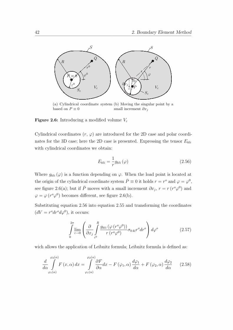
42 2. Boundary Element Method
S
P ≡ 0
Q
r0
ϕ0
R
VεSε
ε0
(a) Cylindrical coordinate systembased on P ≡ 0
S
0
P
Q
r
ϕ
R
Vε
Sε
ε∂xj
(b) Moving the singular point by asmall increment ∂xj
Figure 2.6: Introducing a modified volume Vε
Cylindrical coordinates (r, ϕ) are introduced for the 2D case and polar coordi-
nates for the 3D case; here the 2D case is presented. Expressing the tensor Ekli
with cylindrical coordinates we obtain:
Ekli =1
rgkli (ϕ) (2.56)
Where gkli (ϕ) is a function depending on ϕ. When the load point is located at
the origin of the cylindrical coordinate system P ≡ 0 it holds r = ro and ϕ = ϕ0,
see figure 2.6(a); but if P moves with a small increment ∂xj, r = r (roϕ0) and
ϕ = ϕ (roϕ0) becomes different, see figure 2.6(b).
Substituting equation 2.56 into equation 2.55 and transforming the coordinates
(dV = rodrodϕ0), it occurs:
2π∫0
limε→0
∂
∂xj
R∫ε0
gkli (ϕ (roϕ0))
r (roϕ0)σ0 klr
odro
dϕo (2.57)
wich allows the application of Leibnitz formula; Leibnitz formula is defined as:
d
dα
ϕ2(α)∫ϕ1(α)
F (x, α) dx =
ϕ2(α)∫ϕ1(α)
∂F
∂αdx− F (ϕ1, α)
dϕ1
dα+ F (ϕ2, α)
dϕ2
dα(2.58)

2.3. Integral Formulation 43
Applying this to the term between the brackets of equation 2.57 we obtain:
∂
∂xj
R∫ε0
gkli (ϕ)
rσ0 klr
odro =
R∫ε0
∂
∂xj
gkli (ϕ)
rσ0 klr
odro − gkli (ϕ)
rσ0 klε
0 ∂ε0
∂xj+gkli (ϕ)
rσ0 klR
∂R
∂xj
(2.59)
The last term in equation 2.59 vanishes, because R is independent of xj and
thus ∂R/∂xj = 0. For a detailed proof see Telles (1983), Brebbia et al. (1984).
Substituting this bag into the brackets from equation 2.57 and taking into
consideration that P ≡ 0 and r = ε it arise:
2π∫0
limε→0
R∫ε0
∂
∂xj
gkli (ϕ)
rσ0 klr
odro − gkli (ϕ)
rσ0 klr
∂r
∂xj
dϕo (2.60)
After that, one can transform equation 2.60 back to rectangular coordinates
(with r = r0 and dS = r0dϕo and using equation 2.56):
∂
∂xj
∫V
Ekliσ0 kldV = −∫V
∂Ekli∂xj︸ ︷︷ ︸W εijkl
σ0 kldV −∫Sε
Eklir,jdS
︸ ︷︷ ︸F εijkl
σ0 kl
(2.61)
in which the first integral is interpreted as Cauchy principal value; the last term
F εijkl is called free term.
The term for applying initial strains ε0 kl (the last term of equation 2.53) can
be calculated similar as described above. At the end we obtain:
∂
∂xj
∫V
Rkliε0 kldV =
∫V
∂Rkli
∂xj︸ ︷︷ ︸V εijkl
ε0 kldV −∫Sε
Rklir,jdS
︸ ︷︷ ︸Hεijkl
ε0 kl
(2.62)

44 2. Boundary Element Method
The whole integral equation for strains can be written in compact form:
εij =
∫S
DεkijtkdS −
∫S
SεkijukdS + f εij (2.63)
and
f εij =
∫V
DεkijbkdV +
∫V
W εijklσ0 kldV + F ε
ijklσ0 kl
+
∫V
V εijklε0 kldV +Hε
ijklε0 kl
(2.64)
With
W εijkl =
1
8απG (1− ν) rα+1
[(1− 2ν) (δikδjl + δjkδil)− δijδkl
+ βν (δilr,jr,k + δjkr,ir,l + δikr,jr,l + δjlr,ir,k)
+ β (δklr,ir,j + δijr,kr,l − γr,ir,jr,kr,l)] (2.65)
F εijkl =
−1
2ηG (1− ν)[δjkδil − C1 (δikδjl + δijδkl)] (2.66)
V εijkl =
1
4απ (1− ν) rα+1
[(1− 2ν) (δikδjl + δjkδil − δijδkl)
+ βν (δilr,jr,k + δjkr,ir,l + δikr,jr,l + δjlr,ir,k)
+ β ((1− 2ν) δklr,ir,j + δijr,kr,l − γr,ir,jr,kr,l)] (2.67)
Hεijkl =
−1
η (1− ν)[C1 (δjkδil + δikδjl)− C2δijδkl] (2.68)
With α = 1, β = 2, γ = 4, η = 8, C1 = 3− 4ν, C2 = 1 for 2D (plain strain) and
α = 2, β = 3, γ = 5, η = 15, C1 = 4− 5ν, C2 = 1− 5ν for 3D, see Beer et al.
(2008).

2.3. Integral Formulation 45
Stresses at Internal Points
The stress integral equation can be derived from the strain integral equation by
using following relation:
σij = Cijklεkl (2.69)
Substituting equation 2.63 into equation 2.69 we obtain directly the stress
integral equation. In compact form it can be written as:
σij =
∫S
DσkijtkdS −
∫S
SσkijukdS + fσij (2.70)
and
fσij =
∫V
DσkijbkdV +
∫V
W σijklσ0 kldV + F σ
ijklσ0 kl
+
∫V
V σijklε0 kldV +Hσ
ijklε0 kl
(2.71)
With
Dσijk =
1
4απ (1− ν) rα[(1− 2ν) (δikr,j + δjkr,i − δijr,k) + βr,ir,jr,k] (2.72)
Sσijk =G
2απ (1− ν) rβ[βr,mnm [(1− 2ν) δijr,k + ν (δikr,j + δjkr,i)− γr,ir,jr,k]
+ βν (nir,jr,k + njr,ir,k)
+ (1− 2ν) (βr,ir,jnk + δiknj + δjkni+)− (1− 4ν) δijnk]
(2.73)
W σijkl =
1
4απ (1− ν) rα+1
[(1− 2ν) (δikδjl + δjkδil − δijδkl + βδijr,kr,l)
+ βν (δilr,jr,k + δjkr,ir,l + δikr,jr,l + δjlr,ir,k)
+ β (δklr,ir,j − γr,ir,jr,kr,l)] (2.74)
F σijkl =
−1
αη (1− ν)[C3 (δjkδil + δikδjl) + C4δijδkl] (2.75)

46 2. Boundary Element Method
V σijkl =
g
2απ (1− ν) rα+1
[(1− 2ν) (δikδjl + δjkδil)− (1− 2αν) δijδkl
+ βν (δilr,jr,k + δjkr,ir,l + δikr,jr,l + δjlr,ir,k)
+ β ((1− 2ν) δklr,ir,j + C5δijr,kr,l − γr,ir,jr,kr,l)] (2.76)
Hσijkl =
G
κ (1− ν)[C3 (δikδjl + δjkδil) + C6δijδkl] (2.77)
With α = 1, β = 2, γ = 4, η = 8, C1 = 3− 4ν, C2 = 1 for 2D (plain strain) and
α = 2, β = 3, γ = 5, η = 15, C1 = 4− 5ν, C2 = 1− 5ν for 3D, see Beer et al.
(2008).
2.4 Numerical Implementation
To solve the BIE equation 2.44 numerically, some approximations have to
be introduced. On the one hand the geometry of the problem has to be
approximated numerically, on the other hand also the distribution of physical
quantities (e.g. boundary displacements and boundary tractions) has to be
approximated numerically. Both, the geometry and the physical quantities on
the boundary are approximated by using boundary elements. Applying point
collocation on the element nodes a system of equations can be obtained. In
order to simplify the notation, form now on matrix notation will be used instead
of indicial notation.
2.4.1 Discretisation of the Boundary Geometry
The boundary S of the domain is discretised with boundary elements Se, see
figure 2.7(a).
S ≈E∑e=1
Se (2.78)
where E is the number of boundary elements. For the 2D case we use 1D
boundary elements with two nodes for linear interpolation over the element or
with three nodes for quadratic interpolation over the element.

2.4. Numerical Implementation 47
S ≈∑Se
(a) Discretisation of the boundary S
x2
x1
x3
n = 2 n = 1 n = 3ξ
ξ = −1 ξ = 0 ξ = +1
(b) Quadratic Boundary ele-ment
Figure 2.7: Boundary discretisation in 2D with quadratic elements
Each boundary element is transformed into a local intrinsic coordinate system
(with the intrinsic coordinate ξ), see figure 2.7(b). The coordinate vector xe (ξ)
of any point ξ at the element e can be interpolated by using the interpolation
functions Φn (ξ) and the nodal coordinate vectors of the element xen:
xe (ξ) =Ne∑n=1
Φn (ξ)xen (2.79)
When using 1D quadratic elements we have three nodes at one element (N e = 3)
The interpolation functions are defined to have a unit value at the node n and
a zero value at the other nodes, see figure 2.8:
Φ1 =1
2
(−ξ + ξ2
)Φ2 =
1
2
(ξ + ξ2
)Φ3 = 1− ξ2
(2.80)
For the 3D case 2D boundary elements are used, they can have for example
four nodes N e = 4 (linear interpolation) or eight nodes N e = 8 (quadratic
interpolation). The intrinsic coordinates are ξ and η, see figure 2.9.

48 2. Boundary Element Method
n = 2 n = 1 n = 3
Φ2
Φ1
Φ3
Figure 2.8: Quadratic shape functions for a 1D element
The interpolation functions for a quadratic quadrilateral element are:
Φ1 =1
4(1− ξ) (1− η) (−ξ − η − 1) Φ5 =
1
2
(1− ξ2
)(1− η)
Φ2 =1
4(1 + ξ) (1− η) (ξ − η − 1) Φ6 =
1
2
(1− η2
)(1 + ξ)
Φ3 =1
4(1 + ξ) (1 + η) (ξη − 1) Φ7 =
1
2
(1− ξ2
)(1 + η)
Φ4 =1
4(1− ξ) (1 + η) (−ξ + η − 1) Φ8 =
1
2
(1− η2
)(1− ξ)
(2.81)
and the coordinates for the node at the element xe (ξ, η) can be interpolated as
in equation 2.79:
xe (ξ, η) =Ne∑n=1
Φn (ξ, η)xen (2.82)
For more details and linear interpolation functions see for example Beer and
Watson (1994); for the interpolation of triangular elements see for example Gaul
et al. (2003).

2.4. Numerical Implementation 49
η
ξ
n = 1 25
68
34 7
Figure 2.9: Quadratic quadrilateral element, intrinsic coordinates ξ and η andlocal nodes n = 1...8
2.4.2 Approximation of Physical Quantities
In addition to the discretisation of the boundary geometry, the displacement-
and traction- vectors u and t at the boundary have to be approximated too:
ue =Ne∑n=1
Φnuen (2.83)
te =Ne∑n=1
Φnten (2.84)
where uen and ten are the displacement- and traction- vectors at node n of
element e. And the same interpolation functions Φn as for the geometry in
section 2.4.1 can be used. The fact that the traction interpolation function
is of the same order as the displacement interpolation presents an advantage
over the Finite Element Method, where stresses and tractions are calculated by
differentiation of the displacement interpolation functions and thus results in
loss accuracy.
The BIE involves the three coordinates of the traction vector t at the boundary
nodes; however, the stress tensor has six independent components and three
of them cannot be calculated directly with the BIE; however, the boundary

50 2. Boundary Element Method
stresses cannot be calculated with the integral equation for stresses as well,
because the kernel function Sσijk is hyper singular (see also section 2.4.5). The
most popular and easiest way to compute boundary stresses is the traction
recovery (or stress recovery) method, see for example Gao and Davies (2002),
Brebbia et al. (1984).
2.4.3 Discretisation inside the Domain
S ≈∑Se
V ≈∑V c
Figure 2.10: Domain discretised with integration cells V c
As described before, the boundary geometry and the boundary quantities are
approximated by using boundary elements. However, for a problem containing
body forces (forces, initial stresses or initial strains) domain integrals have to
be computed, see section 2.3.5. One way to calculate the domain integral is the
cell integration technique in which the volume V on which the body forces are
acting is subdivided into a certain number C of cells, see figure 2.10:
V ≈C∑c=1
V c (2.85)
The geometry and the distribution of the body forces are defined by the nodal
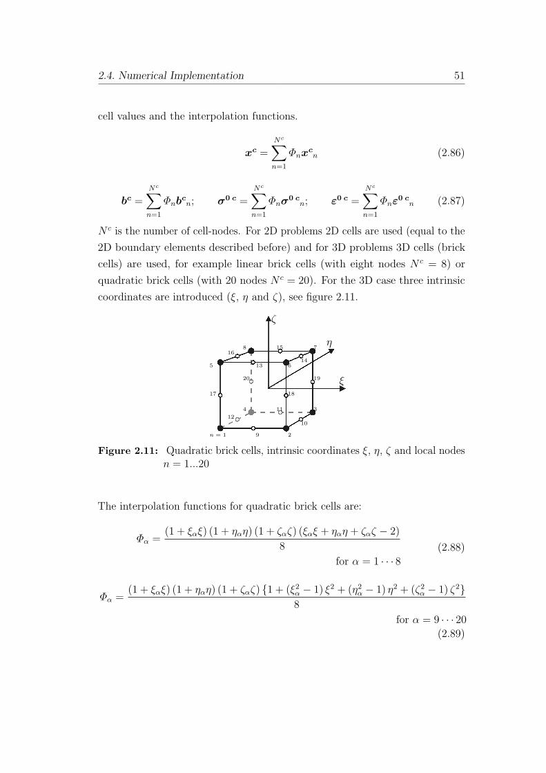
2.4. Numerical Implementation 51
cell values and the interpolation functions.
xc =Nc∑n=1
Φnxcn (2.86)
bc =Nc∑n=1
Φnbcn; σ0 c =
Nc∑n=1
Φnσ0 c
n; ε0 c =Nc∑n=1
Φnε0 c
n (2.87)
N c is the number of cell-nodes. For 2D problems 2D cells are used (equal to the
2D boundary elements described before) and for 3D problems 3D cells (brick
cells) are used, for example linear brick cells (with eight nodes N c = 8) or
quadratic brick cells (with 20 nodes N c = 20). For the 3D case three intrinsic
coordinates are introduced (ξ, η and ζ), see figure 2.11.
ζ
η
ξ
n = 1 29
1012
3114
20
8
19
7
18
6
17
5 13
1516
14
Figure 2.11: Quadratic brick cells, intrinsic coordinates ξ, η, ζ and local nodesn = 1...20
The interpolation functions for quadratic brick cells are:
Φα =(1 + ξαξ) (1 + ηαη) (1 + ζαζ) (ξαξ + ηαη + ζαζ − 2)
8
for α = 1 · · · 8(2.88)
Φα =(1 + ξαξ) (1 + ηαη) (1 + ζαζ) {1 + (ξ2
α − 1) ξ2 + (η2α − 1) η2 + (ζ2
α − 1) ζ2}8
for α = 9 · · · 20
(2.89)

52 2. Boundary Element Method
2.4.4 Matrix Assembly / System of equations
Applying the boundary discretisation (equation 2.78) to the BIE equation 2.44
and expressing it in matrix notation we obtain the equation system for the load
point (subscript l):
clul =E∑e=1
∫Se
U ltedS −
E∑e=1
∫Se
T luedS + f (2.90)
Substituting the displacement- and traction- approximation of equation 2.83
and equation 2.84 into equation 2.90:
clul =E∑e=1
Ne∑n=1
∫Se
U lΦndS︸ ︷︷ ︸∆U e
l n
ten −E∑e=1
Ne∑n=1
∫Se
T lΦndS︸ ︷︷ ︸∆T e
l n
uen + f l (2.91)
Where ∆U el n and ∆T e
l n are introduce to replace the integrands of the products
of the fundamental solution with the shape functions. Replacing the double
summation over the elements E and the element nodes N e by the summation
over all nodes N , it remain:
clul =N∑n=1
∆U l ntn −N∑n=1
∆T l nun + f l (2.92)
In section 2.4.5 it is described how to solve the integrals ∆U l n and ∆T l n
numerically. To setup the entire system of equations for all N unknowns, the
load point (subscript l) is placed at all global discretisation nodes N . The whole
system of equations is:
cu = ∆Ut−∆Tu+ f (2.93)
Where u, t and f are defined to be the global vectors containing the complete
set of N nodal vectors ul, tl and f l. ∆T , ∆U are assembled matrices. By
defining the matrix ∆T in such a way that the free term c is already included,

2.4. Numerical Implementation 53
we obtain:
∆T u = ∆Ut+ f (2.94)
The boundary conditions are imposed by changing columns between the matrices
∆T and ∆U and the following system of equations is obtained:
Ax = b+ f (2.95)
where x contains the unknown boundary values, either tractions t or displace-
ments u; A is a matrix containing a mixture of ∆T and ∆U , related to x;
b contains the contributions due to the known boundary values; and f is a
vector containing the contributions due to the body forces. Assuming a problem
containing all three types of body forces (forces b, initial stresses σ0 and initial
strains ε0), the body force vector given in equation 2.43 can be written in the
form:
f = ∆Ub+ ∆Eσ0 + ∆Rε0 (2.96)
∆U , ∆E and ∆R are the assembled matrices including the integrals of the
products of the fundamental solutions with the shape functions over the cell-
volumes. b, σ0 and ε0 are the global vectors containing the complete set of all
M nodal body force vectors. M is due to the number of cells C and the number
of nodes per cell N c (M = CN c).
The systems of equations for calculating results at interal points (load point is
inside the domain, subscript i) can be expressed in an analogous manner (see
also equation 2.47,equation 2.63 and equation 2.70):
ui = ∆U i t−∆T i u+ f i (2.97)
εi = ∆Dεi t−∆Sεi u+ fε (2.98)
σi = ∆Dσi t−∆Sσi u+ fσ (2.99)
Where the body force vector f i for the displacement results is described in
equation 2.96 and the body force vectors for the strains and for the stresses fε
54 2. Boundary Element Method
and fσ are defined as follows:
fεi = ∆Dεib+ ∆W ε
iσ0 + F εσ0 + ∆V εiε0 +Hεε0 (2.100)
fσi = ∆Dσib+ ∆W σ
iσ0 + F σσ0 + ∆V σiε0 +Hσε0 (2.101)
2.4.5 Numerical Integration
The last thing to do before we are able to operate with the system of equations
in section 2.4.4 is to carry out the integrals over the boundary elements Se
and over the volume cells V c. All these integrals consist of the product of the
fundamental solution (·) (P,Q) and the interpolation functions φ (Q):
Ien (P ) =
∫Se
(·) (P,Q)φn (Q) dS (Q) (2.102)
Icn (P ) =
∫V c
(·) (P,Q)φn (Q) dV (Q) (2.103)
Equation 2.102 shows an integral over a boundary element (like in equation 2.91)
and equation 2.103 shows an integral over a cell. Analytical integration is rarely
used because even when it is possible to calculate the final expression, it can be
very complicated and its evaluation can have high cost from the computational
point of view (see Paris and Canas 1997). Several numerical procedures (e.g.
trapezoidal rule, Simpson’s rule) are described in literature to approximate
an integral like this. However, the Gauss quadrature formula shows the best
accuracy for a given number of points, thus these technique is commonly used
in the BEM.
Depending on the distance of the load point P to the element Se (Q) over which
the integration is carried out, we have to distinguish between regular integrals,
singular integrals and ideally also nearly singular integrals, see for example Gaul
et al. (2003).

2.4. Numerical Implementation 55
Regular Integration
The load point P is far away from the element Se or the cell V c, respectively.
For this the standard Gauss quadrature (also called Gauss-Legendre quadrature)
is used. The original integral can be calculated in the form:
x2∫x1
f (x) dx =M∑j=1
wjf (xj) (2.104)
We can find a set of M weights w and abscissas x (also called Gauss points)
such that the approximation is exact if f (x) is a polynomial of the order R
(M = 2R− 1). Once the order M is chosen, the Gauss points and the weights
can be calculated, for a detailed description see Press et al. (2002). Regarding
a 1D element with the intrinsic coordinates (−1 ≤ ξ ≤ 1) the weights wj and
Gauss points ξj for M = 1, 2, 3 are:
M ξj wj1 0. 2.2 +0.57735, -0.57735 1., 1.3 +0.77459, 0., -0.77459 0.55555, 0.88888, 0.55555
Table 2.1: Gauss points ξ and weights w for Gauss quadrature
Applying this to the integral equation 2.102 it occurs:
Ien (P ) ≈M∑j=1
(·) (P, ξj)φn (ξj) J (ξj)wj (2.105)
where J (ξj) is the Jacobian which transforms the coordinates xj to the intrinsic
coordinates ξj:
dS (x, y) =
√(dx
dξ
)2
+
(dy
dξ
)2
= Jdξ ... 2D boundary element (2.106)

56 2. Boundary Element Method
dS (x, y, z) =∂ (x, y, z)
∂ (ξ, η)= Jdξdη ... 3D boundary element (2.107)
The integration over the volume cells (equation 2.103) can be done analogous:
dV (x, y) =∂ (x, y)
∂ (ξ, η)= Jdξdη ... 2D cell (2.108)
dV (x, y, z) =∂ (x, y, z)
∂ (ξ, η, ζ)= Jdξdηdζ ... 3D cell (2.109)
Nearly Singular Integration
The load point P is close to the element Se or the cell V c, respectively. In this
case, the integrand is still regular and the standard Gauss quadrature formula
can be used. However, a high number of Gauss points xj is needed for an
accurate approximation of the pronounced peak for r (P,Q)�. A better way
to obtain a better accuracy is the subdivision method. If the point is too close to
the element to be integrated, the element is divided into smaller sub-elements,
see Ribeiro (2006).
Singular Integration
When the load point P lies on the element Se or on the cell V c, respectively
the integrand becomes singular for r = 0 (P = Q). Depending on the type of
fundamental solutions different types of singularities occur:
1D Integration 2D Integration 3D Integration
weakly singular ln r1
r
1
r2
strongly singular1
r
1
r2
1
r3
hyper singular1
r2
1
r3
Table 2.2: Different types of singularities

2.4. Numerical Implementation 57
Thus the integrands in the BIE include weak and strong singularities at P = Q:
cu (P ) = ∆U (P,Q)︸ ︷︷ ︸weak
t (Q)−∆T (P,Q)︸ ︷︷ ︸strong
u (Q) + f (P ) (2.110)
and the body force terms consists of weakly singular volume integrals only in
the case that P = Q:
f (P ) = ∆U(P, Q
)︸ ︷︷ ︸weak
b(Q)
+ ∆E(P, Q
)︸ ︷︷ ︸weak
σ0
(Q)
+ ∆R(P, Q
)︸ ︷︷ ︸weak
ε0
(Q)
(2.111)
However, the integral equations for computing stresses or strains consist of
strongly and hyper singular integrals for P = Q:
ε,σ(P)
= ∆Dε,σ(P , Q
)︸ ︷︷ ︸strong
t−∆Sε,σ(P , Q
)︸ ︷︷ ︸hyper
u+ fε,σ(P)
(2.112)
To avoid hyper singular integrals, the integral equation 2.112 is used to calculate
stresses and strains at internal points only. For the boundary we use the stress
recovery technique. Thus we obtain regular boundary integrals only:
ε,σ(P)
= ∆Dε,σ(P , Q
)︸ ︷︷ ︸regular
t−∆Sε,σ(P , Q
)︸ ︷︷ ︸regular
u+ fε,σ(P)
(2.113)
and the volume integrals for the body forces contain strongly singularities at
P = Q:
fε,σ(P)
= ∆Dε,σ(P , Q
)︸ ︷︷ ︸weak
b(Q)
+ ∆W ε,σ(P , Q
)︸ ︷︷ ︸strong
σ0
(Q)
+ F ε,σσ0
(Q)
+ ∆V ε,σ(P , Q
)︸ ︷︷ ︸strong
ε0
(Q)
+Hε,σε0
(Q) (2.114)
The different types of singularities are described in more detail in section 2.5.
However, here a short overview is given, how to integrate them numerically

58 2. Boundary Element Method
inside the BE-program:
Weak Singularity The integral exists and can be calculated analytically (see sec-
tion 2.5.1). The numerical evaluation using the standard Gauss-Legendre
quadrature (section 2.4.5) is inaccurate since the behaviour in the neigh-
bourhood of the singularity can not be approximated very good with
polynomial functions. For the 1D boundary integration a special Gauss
formula the Gauss-Laguerre formula is used, see Beer et al. (2008), Press
et al. (2002).
For 2D and 3D integrations some regularising transformations have to be
considered in which the Jacobian J vanishes at the singularity (e.g. Lachat-
Watson transformation). Quadrilateral elements or cells (2D integration)
have to be subdivided into two triangles. Brick cells (3D integration) have
to be subdivided into pyramid shaped sub-cells. With this subdivisions
new coordinates are introduced and the Jacobian vanishes in the singular
point. For detailed description see for example Ribeiro (2006), Beer et al.
(2008).
Strong Singularity The strongly singular integrals appearing in the BEM exist
in the sense of Cauchy principal values, see section 2.5.2. In the BEM they
often can be evaluated indirectly using the traction-free rigid body motion;
so that the evaluation of the strongly singular integrals can be avoided.
However, in some cases we have to evaluate the strongly singular integrals
explicitly, see Gaul et al. (2003). Therefore different methods can be used
based on analytical or semi-analytical integration. Here the Guiggiani
approach (Guiggiani and Casalini (1987), Guiggiani and Gigante (1990))
is used. This method is based on the idea of regularising the singularity
by subtraction. First we simplify the problem by introducing a function
g (0):
−b∫
a
g (x)
xdx =
∫abg (x)− g (0)
xdx︸ ︷︷ ︸
regular
+ −b∫
a
g (0)
xdx (2.115)

2.4. Numerical Implementation 59
The first integral on the right side is regular and can be evaluated using
standard Gauss quadrature. The second integral remains strongly singular
but its solution is known:
−b∫
a
g (0)
xdx = g (0) ln | b
a| (2.116)
This procedure can be used for 2D and 3D integrations as well.
As for the weak singular integration, the quadrilaterals or bricks are
subdivided into triangular or pyramid shaped sub-elements, respectively.
For example the 2D integration for the strongly singular term ∆T given
by equation 2.91 is expressed in local polar coordinates (ϕ, r) based at
the singular load point P :
∆Tij =N∑e=1
limε→0
∫Se−Sε
TijΦndS =
N∑e=1
limε→0
π∫ϕ= 3
4π
r1(ϕ)∫r0(ε,ϕ)
fij (r, ϕ) rdrdϕ
(2.117)
where Se is the boundary of the element and Sε is the boundary of the
vanishing neighbourhood around the singularity. Then the distance vector
ri is approximated by developing a Taylor series for the field point Q
near the load point. Thus the integrand in the vicinity of the load point
approximate by:
fij (r, ϕ) =1
r2f ∗ij (ϕ) (2.118)
The integrand has been separated into a regular part f ∗ij (ϕ) which is only
a function of ϕ and a singular part 1r2 . Similar to the 1D integration

60 2. Boundary Element Method
function fij (r, ϕ) is subtracted and added:
∆Tij =N∑e=1
π∫ϕ= 3
4π
r1(ϕ)∫0
(fij (r, ϕ)−
f ∗ij (ϕ)
r2
)rdrdϕ
+N∑e=1
limε→0
π∫ϕ= 3
4π
r1(ϕ)∫r0(ε,ϕ)
fij (r, ϕ)f ∗ij (ϕ)
rdrdϕ
(2.119)
where the first integral is regular and can be evaluated using standard
Gauss quadrature. The second integral can be carried out analytically
over r, see Gaul et al. (2003), Ribeiro (2006).
Hyper Singularity As it was shown in equation 2.112 hyper singular integrals
occur when we want to calculate stresses or strains at the boundary. To
avoid this kind of singularity the stresses and strains at the boundary are
not calculated directly by using the integral equations, however stresses
and strains can be computed by using special techniques. The most
popular and easiest way is the traction recovery (or stress recovery, strain
recovery) method, see for example Gao and Davies (2002), Brebbia et al.
(1984).
For a general description of weakly and strongly singular integrals see sec-
tion 2.5.
To apply special kinds of body forces, such as line loads or concentrated point
forces as it is described in section 2.3.5, the singularities have to be considered
in special ways. However, this will be described later in more detail in chapter 5
and chapter 6 where line loads and point forces are used to model different
kinds of rock bolts.

2.5. Singular Integrals 61
2.5 Singular Integrals
For detailed descriptions of singular integrals see for example the mathematics
books Gakkov (1966), Mikhilin and Prossdorf (1987); for a more engineering
description related to the BEM see for example Paris and Canas (1997), Gaul
et al. (2003). In this section short overview over weak and strong singularities
is given.
2.5.1 Weak Singularity
The definition of the weakly singular integral can be given in a visual way (see
Gaul et al. 2003): the integrand is infinite at a point c of the integration range
a ≤ c ≤ b but its integral is finite and continuous at c. See for example the
integrand f (x):
f (x) = ln (|x|) I (x) =
∫f (x) dx = x ln (|x|)− x (2.120)
The integral I (x) is continuous, see figure 2.12
f (x)
I (x)
Figure 2.12: Weak singularity: integrand f (x) and integral I (x)
In mathematics this kind of integral is called improper integral. The integral
is carried out by removing the neighbourhood of the singular point c and
integrating over the remaining part and passing to the limit:
limε1→0; ε2→0
c−ε1∫a
f (x) dx+
b∫c+ε2
f (x) dx
(2.121)

62 2. Boundary Element Method
For the improper integral this limit exists. In this definition it is important
that the neighbourhood cut out is entirely arbitrary (ε1 6= ε2); see for example
Gakkov (1966), Paris and Canas (1997).
2.5.2 Strong Singularity
We have a stong singularity if the integrand is infinite at a point c and its
integral is infinite too. See for example (figure 2.13):
f (x) =1
xI (x) =
∫f (x) dx = ln (|x|) (2.122)
f (x)
I (x)
Figure 2.13: Strong singularity: integrand f (x) and integral I (x)
This kind of integrals can not be solved as an improper integral:
b∫a
1
xdx = lim
ε1→0; ε2→0
−ε1∫a
1
xdx+
b∫+ε2
1
xdx
=
ln
(|b||a|
)+ lim
ε1→0; ε2→0ln
(ε1
ε2
) (2.123)
It is evident that the limit of the last expression depends on the manner in which
ε1 and ε2 tend to zero. However, it can be given a meaning if a dependence
between ε1 and ε2 is established; i.e. ε1 = ε2 = ε. In this example this gives a
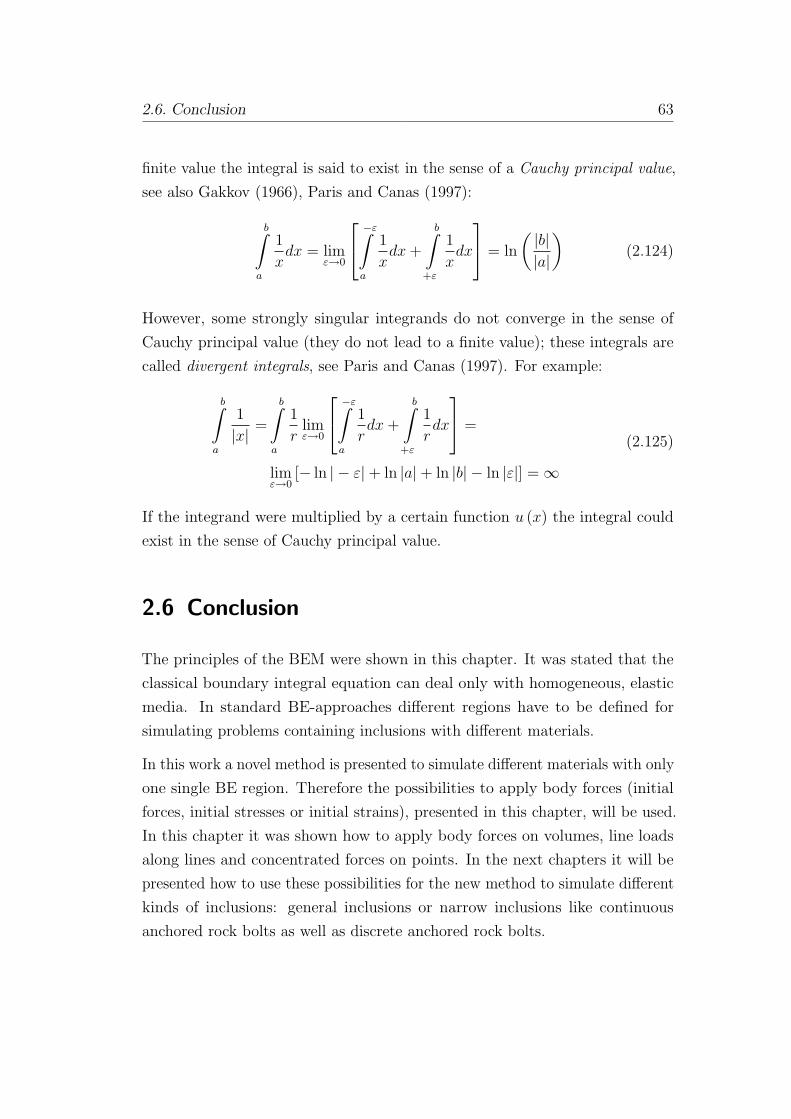
2.6. Conclusion 63
finite value the integral is said to exist in the sense of a Cauchy principal value,
see also Gakkov (1966), Paris and Canas (1997):
b∫a
1
xdx = lim
ε→0
−ε∫a
1
xdx+
b∫+ε
1
xdx
= ln
(|b||a|
)(2.124)
However, some strongly singular integrands do not converge in the sense of
Cauchy principal value (they do not lead to a finite value); these integrals are
called divergent integrals, see Paris and Canas (1997). For example:
b∫a
1
|x|=
b∫a
1
rlimε→0
−ε∫a
1
rdx+
b∫+ε
1
rdx
=
limε→0
[− ln | − ε|+ ln |a|+ ln |b| − ln |ε|] =∞
(2.125)
If the integrand were multiplied by a certain function u (x) the integral could
exist in the sense of Cauchy principal value.
2.6 Conclusion
The principles of the BEM were shown in this chapter. It was stated that the
classical boundary integral equation can deal only with homogeneous, elastic
media. In standard BE-approaches different regions have to be defined for
simulating problems containing inclusions with different materials.
In this work a novel method is presented to simulate different materials with only
one single BE region. Therefore the possibilities to apply body forces (initial
forces, initial stresses or initial strains), presented in this chapter, will be used.
In this chapter it was shown how to apply body forces on volumes, line loads
along lines and concentrated forces on points. In the next chapters it will be
presented how to use these possibilities for the new method to simulate different
kinds of inclusions: general inclusions or narrow inclusions like continuous
anchored rock bolts as well as discrete anchored rock bolts.

64 2. Boundary Element Method

65
Chapter 3
Solution Procedure for Embedded
Inclusions
3.1 Introduction
The analysis of solids including embedded inclusions is a very common problem
in engineering, for example a rock mass with stiff or soft layers which are often
found in underground engineering problems. An other example are solids which
are reinforced by thin inclusions (as rock bolts in tunnelling) or other ground
improvement methods like pipe roofing, where a stiff umbrella-shaped zone is
created inside the grond.
As described in chapter 2 the classical boundary integral equation (BIE) can
deal with homogeneous and linear elastic materials only, since fundamental
solutions are known for homogeneous materials. The boundary element method
(BEM) is already proved suitable for solving homogenous and linear elastic
problems. For problems where the material properties of the solid changes for
example in the case of embedded inclusions or if nonlinear material behaviour
appear, special treatments have to be introduced:
BEM-FEM Coupling: The combination of BEM and FEM is the most com-
monly used technique to treat these cases. The inclusions are modelled with

66 3. Solution Procedure for Embedded Inclusions
finite elements and combined (coupled) with the boundary elements, see fig-
ure 3.1(a). Also if some areas inside the solid become plastic this technique
can be used by discretising these plastic zones with finite elements and the
rest with boundary elements. The philosophy of this technique is to have
the best of each method, Zienkiewicz was the first who presented the “mar-
riage a la mode - The best of both worlds” in his classical paper presented
in Zienkiewicz et al. (1977). Up to now this method is well-established and
an extensive number of research has been done on this subject, see for exam-
ple Beer and Watson (1994), Brebbia et al. (1984), Hagen (2005), Pereira (2008).
BEM-BEM Coupling: Another alternative technique is the BEM sub-region
technique. Where zones with different materials are considered by boundary
element sub-regions which are connected to each other, see figure 3.1(b). Each
region can be assigned different elastic material properties. However, the BEM
regions can not behave in a nonlinear manner, they have to be linear elastic.
One early work presenting an elastic body divided into sub-regions was written
by Lachat and Watson (1976), further works dealing with this problem are for
example Beer (2001), Duenser (2001), Leite and Venturini (2005).
Body force approach: A completely different technique to deal with different
material properties with the BEM is the approach which will be called here
“body force approach” (this can be either an initial stress or an initial strain or
an initial force approach as well). In this method the whole solid is discretised
by one single region and the effects of the zones with different material properties
are simulated by applying body forces of any kind (initial stresses, initial strains
or initial forces), see figure 3.1(c).
In the literature this method is commonly used to simulate nonlinear material
behaviour. The development of simulating nonlinear material behaviour with
the BEM started in the early 1970s. Since that many approaches have been
proposed, see for example Telles (1983), Gao and Davies (2002), Cisilino and
Aliabadi (1998), Ribeiro et al. (2008).

3.2. Body Force Approach 67
(a) BEM-FEM Coupling (b) BEM-BEM Coupling
(c) Body force approach
Figure 3.1: Methods to simulate inhomogeneous domains
In this work a body force approach is proposed, not only for simulating plastic
zones in an homogeneous media as described in various papers, but also for
simulating embedded inclusions. This inclusions can be softer or stiffer than
the surrounding material and they can also plastify, see also Riederer and Beer
(2009).
3.2 Body Force Approach
The idea in this approach is to introduce only one single region and apply initial
loadings or “body forces” (initial stresses, initial strains or initial forces) to
simulate the effect of the different materials, see figure 3.2.
For simulating nonlinear material behaviour like plasticity or visco-plasticity
this method is well known, commonly an initial stress formulation or an initial
strain formulation is used. The varying material properties in the plastic zones
are simulated by initial stresses or initial strains, the magnitudes and the
distribution of these initial loadings are calculated in an iterative procedure.

68 3. Solution Procedure for Embedded Inclusions
In this work embedded inclusions are proposed to be simulated in a similar way.
The system of equations considering some kind of body forces is given as (see
chapter 2):
Ax = b+ f (3.1)
Where is x a vector with the unknown boundary quantities (displacements and
tractions), b is a vector with the contributions due to the known boundary
values, and f is a vector containing the contributions due to the body forces
(e.g. initial stresses σ0).
The system of equations (3.1) can be solved directly to obtain the unknown
boundary values x if the body forces and thus the vector f is known. For the
simulation of inclusions the body forces are unknown at the beginning and
thus the system of equations (3.1) is under-determined and can not be solved
directly.
However, a second condition can be formulated which relates the body forces to
internal results. For example: the relation of the initial stress loadings σ0 and
stress results σ is given by using the constitutive matrices of the domain and
the inclusion material. With this second condition another set of equations are
introduced which leads to a determined problem which can be solved.
This problem can be either solved directly or iteratively. In the next two
sections both approaches are described and at the end their advantages and
disadvantages will be discussed.
Figure 3.2: Simulation of embedded inclusions with initial stresses

3.2. Body Force Approach 69
3.2.1 Direct Solution Procedure
A direct solvable system of equations can be derived by using the BIE, the
integral equation for computing internal results and a second condition for the
relation of body forces and internal results. In general this problem could be
arranged in several variations; body forces can be either, initial stresses, initial
strains or initial forces and also the internal results can vary form stresses, strains
or displacements. Here an initial stress approach in combination with stress
results at internal nodes is used for explanation, but every other assortment
could be used in a similar way.
First the system of equations (see equation 2.95) considering initial stress loading
(f = ∆Eσ0) is rewritten:
Ax−∆Eσ0 = b (3.2)
For a better view over the system of equations equation 3.2 will be presented in
a way in which the sizes of the vectors and matrices are indicated:
[A]ee {x}e − [∆E]ec {σ0}c = {b}e (3.3)
The subscript e represents the total number of degree of freedoms at the
boundary nodes and c is the total number of stress components at the cell
nodes.
The system of integral equations for computing stresses at internal points is
(see also equation 2.99):
[Aσ]ce {x}e −[∆W F
]cc{σ0}c = {σ}c + {bσ}c (3.4)
Whereas ∆W F = ∆W + F includes the integrated fundamental solution and
the jump term. Aσ is a matrix containing sub-matrices ∆D and ∆S related
to the unknown boundary conditions x; and bσ are the contributions due to
the known boundary values.

70 3. Solution Procedure for Embedded Inclusions
Writing both equation 3.3 and equation 3.4 together, it arise a equation system
of the form: [[A]ee [∆E]ec[Aσ]ce
[∆W F
]cc
][{x}e−{σ0}c
]=
[{b}e
{σ}c + {bσ}c
](3.5)
Now another condition has to be found which relates the initial stresses σ0 to
the internal results σ. Therefore following relations are introduced per node:
σIncl = σ (3.6)
σRock = σ+ σ0 (3.7)
σIncl are the stresses in the inclusion and σRock are stresses which would appear
in the solid if there where no inclusion. By introducing the compatibility
condition of the strains (ε = εIncl = εRock) and by using Hooke’s law we
obtain:
ε = CIncl −1
σIncl = CRock −1
σRock (3.8)
Where CIncl and CRock are the constitutive matrices of the inclusion and the
solid material, respectively. With this it occurs:
σRock = CRockCIncl −1
σIncl (3.9)
Substituting equation 3.9 into equation 3.7 and using also the relation in
equation 3.6 it occurs:
CRockCIncl −1
σ = σ+ σ0 (3.10)
This can be arranged for the whole system (for all cell nodes) and the matrix
C1cc is obtained, which gives finally the relation between initial stresses σ0 and
internal results σ:
{σ0}c =([CRock
]cc
[CIncl
]−1
cc− [I]cc
)︸ ︷︷ ︸
[C1]cc
{σ}c (3.11)

3.2. Body Force Approach 71
[I]cc contains assembled identity matrices.
Substituting this additional relation in equation 3.11 into equation 3.5 a directly
solvable system of equations is obtained:[[A]ee − ([∆E]ec [C1]cc)
[Aσ]ce −([
∆W F]cc
[C1cc]− [Icc])]({x}e
{σ]c
)=
({b}e{bσ}c
)(3.12)
Where the vector on the right hand side includes the contributions due to the
known boundary conditions b and bσ; and the vector on the left hand side
contains the unknown boundary conditions x and the unknown stresses at the
cell nodes σ.
3.2.2 Iterative Solution Procedure
Now an alternative solution procedure will be presented, where the unknown
body force term f is calculated iteratively. The system of equations (3.1) is
rewritten here:
Ax = b+ f (3.13)
In contrast to the direct solvable system of equations 3.12 no additional unknowns
arise in the system of equations (3.13) because of the inclusions; the system
itself remains small.
This procedure looks very similar to the iterative procedure used for the nonlinear
material behaviour and thus can easily combined with it. The advantage of this
combination is that both, the solid and the inclusion are able to behave in a
nonlinear manner without producing much additional effort in contrast to the
direct solution procedure of section 3.2.1.
As for the direct solution, also here the problem could be arranged in several
variations of body forces (initial stresses, initial strains or forces) and in several
variations of internal results (stresses, strains or displacements). Below the
procedure will be described in a general way, where different kinds of body force

72 3. Solution Procedure for Embedded Inclusions
loadings can be used and also different kinds of internal results (internal results
are overall indicated by r).
The iteration procedure starts with an initial analysis (subscript j = 0), in
which the solid is assumed to be homogeneous without any inclusion, thus the
body forces are zerro (∆f j=0 = 0).
A∆xj=0 = b (3.14)
After solving 3.14, the results ∆rj at all cell nodes can be obtained. The total
boundary results and internal results are initialised at this stage:
xj=0 = ∆xj=0
rj=0 = ∆rj=0
(3.15)
After this homogeneous initial analysis the iteration procedure starts:
(i) The index for the iteration step is incremented j = j + 1.
(ii) Because of the different materials of the inclusion and the solid, the stresses
are different in both. The results which are calculated before ij−1 may be
incorrect. The error produced in the last analysis can be calculated and
expressed in terms of residual loadings (e.g. residual initial stresses); with
this the residual vector ∆f j is calculated.
(iii) The convergence is checked by comparing the vector-norm of the residuum
‖∆f j ‖ with a given tolerance:
‖∆f j ‖ ≤ tol (3.16)
After the first iteration step (j > 1) the tolerance is defined by a percentage
of the of the fist residuum tol =‖∆f 1 ‖ ε. Whereas ε = 0.01 is in most
cases accurate enough. If the convergence criterion is fulfilled, the iteration
procedure ends here, otherwise it continues with the next step (iv).

3.2. Body Force Approach 73
(iv) The previous calculated residuum is applied to the system of equations as
new right hand side ∆f j:
A∆xj = ∆f j (3.17)
(v) After solving 3.17, the results ∆rj are calculated at all cell nodes.
(vi) The boundary results and the internal results will be updated:
xj = xj−1 + ∆xj
rj = rj−1 + ∆rj(3.18)
(vii) The iteration procedure continues with step (i).
The iterations proceed until convergence is reached in step (iii). The final system
of equations can be written as the sum of the incremental systems:
Axj = b+ f j (3.19)
where f j =∑
∆f j is the sum of all incremental residual vectors.
In the next chapters (chapter 4, chapter 5, chapter 6) the simulation of different
types of inclusions will be described. For each kind of inclusion the procedure
varies a bit: different kinds of cells, of body forces and of internal result types are
used; also the computation of the residuum is done in different ways. However,
the same iteration loop can be used for all this different kinds of inclusions
and they can be calculated at the same time. For this reason cellgroups are
introduced, which combine all cells with the same characteristics (as inclusion
type, material properties and so on).
In addition nonlinear behaviour (like plasticity) may occur even for the solid
or for the inclusion. The iterative procedure for simulation nonlinear material
behaviour is very similar to the iterative procedure used for calculating the
inclusions. The same iteration loop is used for both. For doing this, all plasticity
cells have to be summarized by one cellgroup too. Considering plasticity in the

74 3. Solution Procedure for Embedded Inclusions
BEM is described in various publications, as for example in Telles (1983), Gao
and Davies (2002), Cisilino and Aliabadi (1998), Ribeiro et al. (2008).
Using the concept of the cellgroups, the different methods can be combined into
one iteration loop. For each cellgroup (index CG) the internal results rCG and
the applied body forces can be different; and the residuum can be calculated in
diverse ways. The total residual vector is obtained by the sum over all cellgroup
residual vectors (∆f j =∑
∆fCGj ). The final system of equations is:
Axj = b+∑CG
fCGj (3.20)
The itrative solution procedure using as many cellgroups as desired, is presented
in figure 3.3.
Iterative Procedure and Coupling
For the simulation of tunnelling problems the coupling of different regions is
in most cases indispensable. For example the simulation of the excavation
process in tunnelling, where the solid around the tunnel is defined by an infinite
BE-region and the solid inside the tunnel surface is subdivided in several finite
BE-regions. The excavation process is simulated, by deactivating the finite
regions step by step, see Duenser (2001). Another example for coupled problems
in tunnelling is the simulation of shotcrete along the tunnel surface. The thin
shotcrete shell can be simulated efficiently with shell elements, see Prazeres
(2009); however this FE’s has to be coupled to the BE-region.
Thus, the iteration procedure described above has to be extended to coupled
problems. The procedure is shown in figure 3.4, the index SYS denotes the
whole system with all regions.

3.2. Body Force Approach 75
Figure 3.3: Flow chart of the iterative algorithm

76 3. Solution Procedure for Embedded Inclusions
Figure 3.4: Flow chart of the iterative algorithm for coupled problems
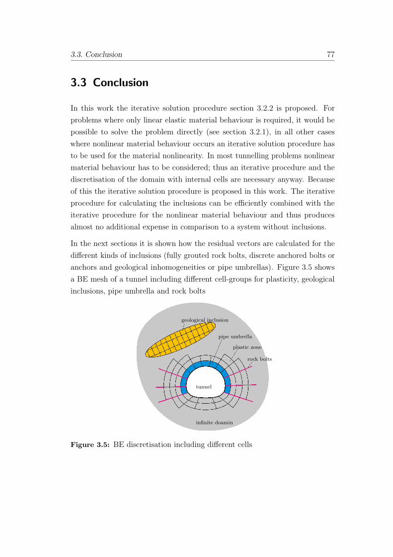
3.3. Conclusion 77
3.3 Conclusion
In this work the iterative solution procedure section 3.2.2 is proposed. For
problems where only linear elastic material behaviour is required, it would be
possible to solve the problem directly (see section 3.2.1), in all other cases
where nonlinear material behaviour occurs an iterative solution procedure has
to be used for the material nonlinearity. In most tunnelling problems nonlinear
material behaviour has to be considered; thus an iterative procedure and the
discretisation of the domain with internal cells are necessary anyway. Because
of this the iterative solution procedure is proposed in this work. The iterative
procedure for calculating the inclusions can be efficiently combined with the
iterative procedure for the nonlinear material behaviour and thus produces
almost no additional expense in comparison to a system without inclusions.
In the next sections it is shown how the residual vectors are calculated for the
different kinds of inclusions (fully grouted rock bolts, discrete anchored bolts or
anchors and geological inhomogeneities or pipe umbrellas). Figure 3.5 shows
a BE mesh of a tunnel including different cell-groups for plasticity, geological
inclusions, pipe umbrella and rock bolts
geological inclusion
pipe umbrella
plastic zone
rock bolts
tunnel
infinite doamin
Figure 3.5: BE discretisation including different cells

78 3. Solution Procedure for Embedded Inclusions

79
Chapter 4
General Inhomogeneities and Pipe
Umbrellas
4.1 General
Usually the ground will not be homogeneous and the simulation program should
be able to consider this. In tunnelling problems different types of inclusions
occur; on the one hand inclusions arise from the geology like fault zones and
soft or stiff layers; on the other hand inclusions are placed in to support the
excavated tunnel, for example rock bolt, anchors, pipe umbrella systems ...
As described in chapter 2 the classical BIE can deal with homogeneous, linear-
elastic domains only. However, in chapter 3 a possibility was presented to
simulate inclusions by applying body forces (e.g. initial stresses) calculated
within an iterative procedure. In this chapter the approach for simulating
geological inclusions and pipe umbrella systems will be presented.
4.1.1 General Inhomogeneities
The calculation of inclusions with arbitrary shape, like geological inhomo-
geneities, can be done within the iterative procedure described in chapter 3.
The inclusions are modelled by ordinary volume-cells, see figure 4.1.

80 4. General Inhomogeneities and Pipe Umbrellas
volume-cells
boundary elements
Figure 4.1: Geological inclusion discretised with cells
4.1.2 Pipe Umbrellas
Technique
To improve the behaviour of the ground and for the stabilisation of the excavated
area, especially the working face, a grouted pipe-roofing technique can be used.
In this technique a series of pipes are installed and after that grout is injected
through the pipes. Thereby the properties of the ground between the pipes are
changed and the pipes are connected to a kind of umbrella around the area to
be excavated, see figure 4.2.
pipegrout
tunnel tunnel
pipe grout
Figure 4.2: Grouted pipe roofing technique

4.1. General 81
Numerical Simulation
Such a pipe-roofing technique described before is a geometrically and mechani-
cally complex problem. In this work it is proposed to approximately simulate
this problem by a homogenized zone. Consequently, the same volume-cells and
the same algorithm as for the general inhomogeneities can be used; one single
layer of ordinary volume-cells is used for discretisation, see figure 4.3.
homogenized zone
tunnel tunnel
homogenized zone
Figure 4.3: Approximated modelling of pipe roofs

82 4. General Inhomogeneities and Pipe Umbrellas
4.2 BE-approach
The general procedure described in section 3.2.2 is adapted to model geological
inhomogeneities. For this, the following special configurations are used:
• General volume-cells are used for discretisation: in 2D problems we have
quadratic quadrilateral cells, in 3D problems quadratic brick cells (see
section 2.4.3).
• Initial stresses σ0 are applied as loading in the volume-cells.
• Internal strain results ∆εj are use for computing the residuum in the j-th
iteration step, see section 4.2.2.
• The residual-vector is computed as described in section 4.2.3.
4.2.1 Iterative Procedure
The iterative procedure is used, as described in section 3.2.2.
First the homogeneous elastic problem is solved:
A∆xj=0 = b (4.1)
After that the strain results ∆εj=0 are calculated at all cell nodes. The total
boundary results and internal results are initialised:
xj=0 = ∆xj=0
εj=0 = ∆εj=0
(4.2)
Then the iteration starts and following steps have to be done:
(i) The index for the iteration step is incremented j = j + 1.
(ii) The residual vector ∆f j is calculated, see section 4.2.3.

4.2. BE-approach 83
(iii) The convergence is checked by comparing the vector-norm of the residuum
‖∆f j ‖ with a given tolerance:
‖∆f j ‖ ≤ tol (4.3)
After the first iteration step (j > 1) the tolerance is defined by a percentage
of the fist residuum tol =‖∆f 1 ‖ ε. If the convergence criterion is fulfilled,
the iteration procedure ends here, otherwise it continues with the next
step (iv).
(iv) The residual vector is applied to the system of equations as new right
hand side:
A∆xj = ∆f j (4.4)
(v) The strain results ∆εj are calculated at all cell nodes.
(vi) The boundary results and the strain results are updated:
xj = xj−1 + ∆xj
εj = εj−1 + ∆εj(4.5)
(vii) The iteration procedure continues with step (i).
4.2.2 Computation of the Strains
Internal strain results (∆εj) are needed for the computation of the residuum.
Between two materials (like the ground and the inclusion) a jump arises in
the stress-field. Because of this discontinuity the strains cannot be calculated
directly by using the integral equation (see equation 2.63). For points inside one
material (even if they are very near to the border) the integral equation 2.63
gives the correct results; but not for points located directly on the border. We
have two options to compute strains at these nodes:
• For nodes located on the border to an other material, the strains are
extrapolated from strain results of points inside the material.

84 4. General Inhomogeneities and Pipe Umbrellas
• The other option is to calculate displacements at all cell nodes by using
the integral equation 2.47. This can be done without problems, because
the displacements do not have a jump at the border between two materials.
Afterwards the strains are calculated for each cell by the derivation of the
displacements (via the interpolation function of the cell).
In this work the second option (derivation of the displacements) is used for
calculating the strains. Thus, this option is described in more detail:
The displacements over the cell are approximated using the interpolation func-
tions Φn and the nodal displacements ucn, see section 2.4.3:
uc =Nc∑n=1
Φnucn (4.6)
The strains for a one dimensional problem can be expressed by the derivative of
the interpolation functions:
ε =∂uc
∂x=
Nc∑n=1
∂Φn∂x
ucn (4.7)
For the general 2D or 3D case this can be written in matrix form:
ε =Nc∑n=1
Bcnu
cn (4.8)
WhereBcn is a matrix containing the derivation of the interpolation functions:
Bcn =
∂Φn∂x
0
0 ∂Φn∂y
∂Φn∂y
∂Φn∂x
for 2D (4.9)

4.2. BE-approach 85
Bcn =
∂Φn∂x
0 0
0 ∂Φn∂y
0
0 0 ∂Φn∂z
∂Φn∂y
∂Φn∂x
0
0 ∂Φn∂z
∂Φn∂y
∂Φn∂z
0 ∂Φn∂x
for 3D (4.10)
4.2.3 Computation of the Residuum
The residual initial stresses ∆σ0j for one iteration step j are calculated by using
the strain results ∆εj and the generalised Hooke’s law for the two different
materials. In order to get a better convergence, different methods are used for
the cases when the inclusion material is softer than the rock mass or when it is
stiffer.
After the residual initial stresses ∆σ0j are calculated at all cell nodes, the
residual vector ∆f j can be computed (see equation 2.43):
∆f j =
∫V
E∆σ0jdV (4.11)
Soft Inclusions
If the inclusion material is soft compared to the rock mass (for example soft
layers), the residual initial stresses are computed by:
∆σ0j =(CRock −CIncl
)∆εj−1 (4.12)
CRock and CIncl are the constitutive matrices of the rock-material and the
inclusion-material, respectively. Equation 4.12 is appropriate to calculate soft
inclusions; because the strains ∆εj−1 are related to the rock mass (which is
stiffer than the inclusion), see figure 4.4.

86 4. General Inhomogeneities and Pipe Umbrellas
Hard Inclusions
If the inclusion is harder than the surrounding solid (as it is the case for pipe
umbrellas) the residual stress computed with equation 4.12 would be very high
and the iteration would not converge in many cases. For this, the residual
stresses are computed in an alternative way:
∆σ0j =(CRock −CIncl
)∆εInclj−1 (4.13)
∆εInclj−1 means that the strains are related to the inclusion material:
∆εInclj−1 = CIncl−1∆σInclj−1
= CIncl−1 (∆σRockj−1 −∆σ0j−1
)= CIncl−1 (
CRock∆εj−1 −∆σ0j−1)) (4.14)
The difference of both variants are schematically shown in figure 4.4. In order to
get convergence in the iteration procedure, the strains are related to the harder
material in each case, thus the residual initial stresses are not too high.
hard inclusion rock mass
rock mass soft inclusion
∆ε ∆ε
∆σ ∆σ
∆εIncl = f`∆σIncl
´∆ε = f
`∆σRock
´
∆σIncl ∆σRock
∆σRock ∆σIncl
∆σ0 ∆σ0
Figure 4.4: Schematic diagram for computing the residuum for soft and hardinclusions

4.2. BE-approach 87
Inclusion with Nonlinear Material
For a problem where the inclusion material behaves nonlinear (e.g. it plastifies)
the residual initial stress consists of two parts: the elastic part σe0 and the
plastic part σp0, see figure 4.5:
σ0 = σe0 + σp0 (4.15)
The elastic part is computed as described before; with this the situation of an
elastic inclusion is obtained (see equation 4.16). The plastic part is computed
starting from the elastic inclusion state σIncl e, see equation 4.17; the plastic
part can be calculated as described in various publications, see for example
Telles (1983), Gao and Davies (2002), Ribeiro et al. (2008).
σIncl e = σRock + σe0 (4.16)
σIncl = σIncl e + σp0 = σRock + σ0 (4.17)
σ
σRock
σIncl e
σIncl
εε
σ
σp0
σe0
σ0
Figure 4.5: Schematic figure of the stress states for inclusions with nonlinearmaterial behaviour

88 4. General Inhomogeneities and Pipe Umbrellas
4.2.4 Evaluation of the Integral
In order to achieve the residual vector ∆f j an integration over the volume-cells
has to be carried out, see equation 4.11. This is done in the standard way as
described in section 2.4.5.

4.3. Verification Examples 89
4.3 Verification Examples
Some very simple examples are presented to verify the described method. Soft,
elastic or plastic inclusions have been tested in 2D and 3D examples. A soft
inclusion in combination with multiple regions has been tested as well; and also
a stiff inclusion and changing material properties within different calculation
steps has been tested.
4.3.1 Example 1: Soft inclusion in plane strain
The first example shows a block with a soft inclusion in plane strain. The
dimension of the block is 2m x 2m; the Young’s modulus is E=5000MN/m2;
and the Poisson’s ratio is ν=0.3. The block is fixed at the bottom and on the
top of the block a constant pressure is applied p=1MN/m2.
Three calculations were carried out: the first without an inclusion; the second
with an elastic inclusion and the third with an inclusion with nonlinear material
behaviour. The soft inclusion has a square shape, placed in the centre of the
block; its dimension is 1m x 1m. The elastic material properties for the inclusion
in the second and the third calculation are: Young’s modulus E=2500MN/m2;
Poisson’s ratio ν=0.3. For the third calculation the Drucker Prager yield
criterion is used with an associated flow rule; the cohesion is c=0.1MN/m2 and
the friction angle is Φ=30◦.
The results are compared with reference solutions calculated with the same
BE-program but with multiple regions (BEM MR); where the inclusion is defined
as an own region. The third calculation is also compared with results from a
FE-analysis. The results are presented in figure 4.6 and figure 4.7.

90 4. General Inhomogeneities and Pipe Umbrellas
Figure 4.6: Example 1: vertical displacements on the top of the block
Figure 4.7: Example 1: deformed mesh and contours of vertical displacements

4.3. Verification Examples 91
4.3.2 Example 2: Soft inclusion in 3D
This example shows a 3D block with a soft inclusion. The dimension of the block
is 10m x 10m x 10m; the Young’s modulus is E=5000MN/m2; and the Poisson’s
ratio is ν=0.0. The block is fixed at the bottom and a constant pressure is
applied at the top of the block p=50MN/m2.
Three calculations were carried out: the first without an inclusion and the
second with an soft elastic inclusion and the third with a plastic inclusion. The
inclusion is placed in the centre of the block and has the dimensions 4m x 4m
x 4m. The elastic material properties of the inclusion are: Young’s modulus
is E=2000MN/m2; Poisson’s ratio is ν=0.3. And for the third calculation the
Drucker Prager yield criterion is used with an associated flow rule; the cohesion
is c=5.0MN/m2; the friction angle is Φ=30◦.
The deformed mesh with the contours of the vertical displacements are shown
in figure 4.8. The results are compared with those calculated with the FEM,
see figure 4.9 and figure 4.10.
Figure 4.8: Example 2: deformed mesh and contours of vertical displacements

92 4. General Inhomogeneities and Pipe Umbrellas
Figure 4.9: Example 2: vertical displacements along the top of the block
Figure 4.10: Example 2: vertical displacements along the top of the inclusion

4.3. Verification Examples 93
4.3.3 Example 3: Soft inclusion and multiple regions
The third example shows again a block with a soft inclusion in plane strain
conditions, but it exhibits the compatibility of this algorithm with multiple
region problems. Two variational calculations have been carried out to calculate
the same problem. The first is with a single region; and the second with two
regions where the splitting is directly in between the inclusion. Both calculations
show good agreement for the displacement results but also for the stress results,
see figure 4.11 and figure 4.12.
The dimension of the block is 2.167m x 2m; the Young’s modulus is E=5000MN/m2;
and the Poisson’s ratio is ν=0.0. The block is fixed at the bottom and on the
top of the block a constant pressure is applied p=1MN/m2. The inclusion
has a dimension of 1m x 1m; the Young’s modulus is E=500MN/m2; and the
Poisson’s ratio ν=0.0.
(a) Single region (b) Two regions
Figure 4.11: Example 3: deformed shape and displacement contours

94 4. General Inhomogeneities and Pipe Umbrellas
(a) Single region (b) Two regions
Figure 4.12: Example 3: deformed shape and contours of vertical stresses
4.3.4 Example 4: Cantilever with stiff inclusion in second
analysis step
The last example is testing a stiff inclusion (modelled by one layer of cells) wich
is under bending load. This shows the applicability of this method to model
pipe umbrellas within a strongly reduced example. In a first step a homogeneous
cantilever beam is loaded over the entire length with a constant pressure; after
that in a second step, an additional loading is applied and the material in the
upper part of the cantilever is changing to be stiffer then before. This stiffer
part is modelled by one layer of inclusion cells, see figure 4.13. The results are
compared with those calculated by the FEM, see figure 4.14.
The cantilever is 10m long and 2m high; it is fixed at the left side and loaded
with a constant pressure along the whole length (in the first step the pressure is
p=5MN/m2 and in the second step an additional pressure of p=5MN/m2 is
applied). The Young’s modulus of the cantilever is E=10000MN/m2 and the
Poisson’s ratio is ν=0.3. In the second step a stiffer zone in the upper part of
the cantilever is introduced, it has a high of 0.5m and the Young’s modulus is
E=50000MN/m2 and the Poisson’s ratio is ν=0.3.

4.3. Verification Examples 95
Figure 4.13: Example 4: deformed mesh after the second calculation step
Figure 4.14: Example 4: vertical displacements along the top of the cantilever

96 4. General Inhomogeneities and Pipe Umbrellas

97
Chapter 5
Continuous Anchored Bolts
5.1 General
In conventional tunnel excavation rock bolts, especially in combination with
shotcrete lining are the most important support elements (see section 1.2). For
different needs a wide variety of bolt types have been developed which are used
in mining and civil engineering. The different kinds of bolts can be assigned
into two main groups: the continuous anchored bolts (or dowels); and the
end-anchored or discrete anchored bolts, see Hoek et al. (1997). In this chapter
the modelling of the first of these groups (the continuous anchored bolts) is
described. The numerical modelling of the second group (the discrete anchored
bolts) will be described in chapter 6.
Technique
Continuous anchored rock bolts generally consist of deformed steel bars which
are grouted into the rock. Pre-stressing of the bolt is not possible and the
loads in the bolts are generated by movements in the rock mass. In order
to be effective, these kind of rock bolts have to be installed before significant
movements in the rock mass has taken place, see Hoek et al. (1997). Figure 5.1
shows different types of typical bolts which can be used in tunnelling.

98 5. Continuous Anchored Bolts
(a) Grouted dowel (b) Grouted cable
(c) Swellex dowel
Figure 5.1: Different types of continuous anchored bolts, see Hoek et al. (1997)
Numerical Simulation
Fully grouted rock bolts (or rock bolts which are in continuous contact with
the ground) could be treated like general inclusions (see chapter 4). However,
because of their narrow geometry it is reasonable to introduce some simplifica-
tions. A number of special BE-formulations have been developed in the past,
for simulating problems containing thin inclusions inside a solid such as piles,
reinforcements or rock bolts, see also Riederer et al. (2009).
Most of the approaches use BEM-FEM coupling, where the solid is modelled
with boundary elements and the thin inclusions are considered by using finite
elements. The coupling is done by enforcing displacement compatibility and
traction equilibrium at the interface nodes between inclusion and solid. Such
inclusions have been modelled in various degrees of simplification: as simple truss

5.1. General 99
elements, as beam elements, or as general volume elements. For the simulation
of very thin inclusions such as reinforcement or rock bolts the bending stiffness
can be neglected and truss elements are used (see for example: Coda 2001,
Leite et al. 2003, Leite and Venturini 2005). For simulating the behaviour of
inclusions where the bending stiffness is taken into account such as for piles,
beam elements are used (see for example: Coda and Venturini 1999, Filho et al.
2005, Padron et al. 2007, Leite and Venturini 2005).
Some papers use pure BEM formulations, where the inclusion is also discretised
with boundary elements (for example in: Banerjee 1981, Wang and Gao 1998,
Maeso et al. 2005, Aliabadi and Saleh 2002, Ma et al. 2008).
In all these approaches the problem is solved directly and therefore additional
unknowns are introduced for the inclusions. Because of this, the size of the
system of equations increases with the number of inclusions.
The goal of this work was to efficiently calculate a very high number of thin linear
inclusions (rock bolts) with a pure BEM and in combination with nonlinear
material behaviour of the rock mass. Because of this a complete new approach
has been developed which solves the problem iteratively.
It is assumed that the rock bolts are in continuous contact with the ground and
that they are sufficiently thin, so that their bending stiffness can be neglected;
they are only able to carry axial stresses. They are modelled by simple line-
cells.

100 5. Continuous Anchored Bolts
5.2 BE-approach
In order to simulate the continuous anchored bolts, the general procedure
described in section 3.2.2 is adapted for these kind of problem, see also Riederer
et al. (2009). Following configurations are used:
• Line-cells are used for the discretisation, see section 5.2.2.
• Axial initial stresses σ0 xx are applied as loading along the line-cells.
• Internal stress results in axial direction of the bolt σxx are use for compu-
tation, see section 5.2.3.
• The residual-vector is computed as described in section 5.2.4.
5.2.1 Iterative Procedure
First the homogeneous elastic problem is solved:
A∆xj=0 = b (5.1)
Then the stresses in axial direction of the bolt ∆σxxj are calculated at all
cell nodes. The total boundary results xj=0 and internal results σxxj=0 are
initialised:xj=0 = ∆xj=0
σxxj=0 = ∆σxxj=0
(5.2)
The iteration starts and following steps have to be done:
(i) The index for the iteration step is incremented j = j + 1.
(ii) The residual vector ∆f j is calculated, see section 5.2.4.
(iii) The convergence is checked by comparing the vector-norm of the residuum
‖∆f j ‖ with a given tolerance:
‖∆f j ‖ ≤ tol (5.3)
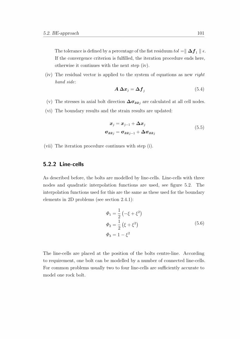
5.2. BE-approach 101
The tolerance is defined by a percentage of the fist residuum tol =‖∆f 1 ‖ ε.If the convergence criterion is fulfilled, the iteration procedure ends here,
otherwise it continues with the next step (iv).
(iv) The residual vector is applied to the system of equations as new right
hand side:
A∆xj = ∆f j (5.4)
(v) The stresses in axial bolt direction ∆σxxj are calculated at all cell nodes.
(vi) The boundary results and the strain results are updated:
xj = xj−1 + ∆xj
σxxj = σxxj−1 + ∆σxxj(5.5)
(vii) The iteration procedure continues with step (i).
5.2.2 Line-cells
As described before, the bolts are modelled by line-cells. Line-cells with three
nodes and quadratic interpolation functions are used, see figure 5.2. The
interpolation functions used for this are the same as these used for the boundary
elements in 2D problems (see section 2.4.1):
Φ1 =1
2
(−ξ + ξ2
)Φ2 =
1
2
(ξ + ξ2
)Φ3 = 1− ξ2
(5.6)
The line-cells are placed at the position of the bolts centre-line. According
to requirement, one bolt can be modelled by a number of connected line-cells.
For common problems usually two to four line-cells are sufficiently accurate to
model one rock bolt.

102 5. Continuous Anchored Bolts
0
2
1
xy
−ξ
ξ
Figure 5.2: Line-cells with three nodes and quadratic interpolation
In order to model these bolts by simple line-cells, some simplifications have to
be introduced. It is assumed that the bolts are sufficiently thin, so that their
bending stiffness can be neglected and that the cross-section is circular and
constant over the length.
Intial axial stresses σ0 xx are applied as loading along these line-cells to simulate
the effect of the bolts inside the rock mass.
5.2.3 Computation of Stresses in Axial Bolt Direction
The internal results needed for the computation of the residuum in the iterative
procedure (section 5.2.1) are the stresses in axial bolt direction ∆σxxj. These
results have to be calculated at all line-cell-nodes. It is possible to compute
displacements or stresses directly at the cell-nodes, in spite of the singularities
(see section 5.2.5).
Therefor we have two possibilities:
• Stress based computation: The stresses are calculated directly by using
the integral equation for stresses at internal points (and stress recovery at
the boundary). Afterward these stress results are transformed into local
coordinate system of the line-cell to obtain the axial stress ∆σxxj at each
node.

5.2. BE-approach 103
• Displacement based computation: The displacements are calculated by us-
ing the integral equation for displacements at internal points (the boundary
displacements are already achieved from the BIE). These displacements
are transformed into the local coordinate system of the line-cell to obtain
the axial displacements ∆uxj at each node. The axial stresses are calcu-
lated from the displacements by using the derivative of the interpolation
functions and Hooke’s law.
Regarding only the rock bolt oneself, in generally the stress based computation
might be the better one, because no derivation of the interpolation function
is necessary and thus it is the more accurate method. However, regarding the
rock bolt computation together with other methods (like the plasticity or the
inclusion calculation) one of both computation methods can be more efficient
than the other one. For example when using rock bolts and inclusions (see
chapter 4) at the same time and using some equal nodes for both, it might be
the best way to use the displacement based computation for the rock bolts,
since the displacement results are needed anyway for the inclusion algorithm
and thus produce no additional effort.
For this work both methods have been implemented into the program BEFE++,
in order to choose the most efficient or most accurate computation for each
example. Thus, both methods will be described in the following in more detail.
Stress Based Computation
As described before, for this computation method the stresses are calculated
at all cell nodes. Stresses at internal nodes are calculated with the integral
equation 2.70, at the boundary nodes the stress recovery method is used. After
that, the stresses are transformed into the local coordinate system of the cell.
For doing so the transformation matrix Tσ for stresses is introduced, see Beer
et al. (2008):
Tσ =
[Tσ11 Tσ12
Tσ21 Tσ22
](5.7)

104 5. Continuous Anchored Bolts
Tσ11 =
s21x s2
2x s23x
s21y s2
2y s23y
s21z s2
2z s23z
Tσ12 =
2s1xs2x 2s2xs3x 2s1xs3x
2s1ys2y 2s2ys3y 2s1ys3y
2s1zs2z 2s2zs3z 2s1zs3z
Tσ21 =
s1xs1y s2xs2y s3xs3y
s1ys1z s2ys2z s3ys3z
s1xs1z s2xs2z s3xs3z
Tσ22 =
s1xs2y + s1ys2x s2xs3y + s2ys3x s1xs3y + s1ys3x
s1ys2z + s1zs2y s2ys3z + s2zs3y s1ys3z + s1zs3y
s1xs2z + s1zs2x s2xs3z + s2zs3x s1xs3z + s1zs3x
(5.8)
s1, s2, s3 are the unit vectors in the directions of the locals coordinate system
of the bolt, see figure 5.3. The stresses in local directions σ can be written as:
σ = Tσσ (5.9)
z
y
x
s3
s2
s1
0
2
1
x, ξ
Figure 5.3: Local coordinate system of a bolt in 3D
Here we need only the axial stress σxx, which is the first entry in the vector σ.
This can be described by introducing the vector vT = [1 0 0 0 0 0]; with this

5.2. BE-approach 105
the axial stress is given by:
σxx = vT (Tσσ) (5.10)
Displacement Based Computation
After the displacements are computed at all points, they are transformed into
the local coordinate systems of the cells:
ux = s1Tu = s1xux + s1yuy + s1zuz (5.11)
where s1 is the unit vector in local bolt direction x, see figure 5.3.
The strains in the cell are computed by using the derivatives of the displace-
ments:
εxx =duxdx
=duxdξ
dξ
dx(5.12)
where ξ is the local intrinsic coordinate of the line-cell. Additional, the interpo-
lation over the nodal displacements and the definition of the Jacobian J are
introduced:
ux =Nc∑n=1
Φnuxn ; J =dx
dξ(5.13)
For the three node line-cell we have N c = 3, the interpolation functions are
specified in equation 5.6. Substituting this into equation 5.12 it occurs:
εxx =Nc∑n=1
dΦndξ
uxnJ
(5.14)
The derivations of the interpolation functions (equation 5.6) can be easily
obtained:dΦ1
dξ= ξ − 1
2dΦ2
dξ= ξ +
1
2dΦ3
dξ= −2ξ
(5.15)

106 5. Continuous Anchored Bolts
At the end the stresses for the cell-nodes are obtained:
σxx = ERockεxx − σ0 xx
= ERock
Nc∑n=1
dΦndξ
uxnJ− σ0 xx
(5.16)
5.2.4 Computation of the Residuum
To compute the residuum ∆f j in the j-th iteration step, first residual initial
stresses ∆σ0 xxj in axial bolt direction x have to be found. If the residual
initial stresses are calculated at all cell nodes, the residual vector ∆f j can be
computed (see equation 2.43 and equation 2.46):
∆f j =C∑c=1
∫Lc
E∆σ0 xxjdx (5.17)
where C is the number of line-cells and Lc is the length of the line-cell c.
The residual inital stresses for the iteration step j are calculated by using the
axial stress results ∆σxxj and the Hooke’s law. The relation between axial
stress in the bolt σBoltxx , the axial stress in the rock σRockxx and the loading (the
axial initial stresses σ0 xx) is shown in figure 5.4; see also:
σBoltxx = σxx
σRockxx = σxx + σ0 xx
(5.18)
To achieve this relation, the residual initial stress is obtained in each iteration
step j. Again we have two alternative ways for computing the residual stresses:
In the first way the incremental results ∆σxxj are used for computation and
in the second way the total results σxxj are used. At the end both alternatives
lead to the same solution.

5.2. BE-approach 107
σ0
σRock = σ + σ0
σBolt = σ
Figure 5.4: Schematic illustration of the stresses in the rock, in the bolt andthe initial stresses (σRockxx , σBoltxx and σ0 xx).
• Incremental calculation: The residual stress is calculated by the difference
of the incremental rock stress and the incremental bolt stress:
∆σ0 xxj = ∆σRock∗
xxj−∆σBoltxxj
(5.19)
∆σRock∗
xxjis the expected rock stress, calculated from the bolt stress and
the relations of the Young’s modulus.
∆σRock∗
xxj= ∆σxxj
ERock
EBolt(5.20)
where ERock and EBolt are the Young’s modulus of the rock and the bolt,
respectively. At the end one obtains:
∆σ0 xxj = ∆σxxj
(ERock
EBolt− 1
)(5.21)
• Total calculation: The residual stress is calculated by the difference of the
total calculated rock stress σRockxxjto the total expected rock stress σRock
∗xxj
(which is computed from the bolt stress):
∆σ0 xxj = σRock∗
xxj− σRockxxj
(5.22)

108 5. Continuous Anchored Bolts
σRock∗
xxjis defined analogous to equation 5.20; with this we obtain:
∆σ0 xxj =σBoltxxj
ERock
EBolt− σRockxxj
=σxxjERock
EBolt−(σxxj − σ0 xxj
) (5.23)
Yielding Bolts
The rock bolt behaviour depends on the behaviour of the steel bar and the
connection of the bar to the surrounding rock mass. Here idealized constitutive
laws for modelling both of these components are presented. The steel bar is
assumed to behave linear elastic up to a defined yield-stress and then perfectly
plastic. The yield stress in the bolt σBolt Y has to be defined and with this the
residual initial stress can be checked and modified if necessary:
σBoltxxj+1= σBoltxxj
− σ0 xxj
if σBoltxxj+1≤ σBolt Y → ok
if σBoltxxj+1> σBolt Y → ∆σ0 xxj = σBoltxxj
− σBolt Y
(5.24)
If the yield stress in the bolt is reached, the residual initial stress σ0 xxj calculated
before (in equation 5.19 or equation 5.22) is corrected, see also figure 5.5. In gen-
eral the yield stress should be compared with the effective stress state (including
not only the axial stresses). However, here in this work the yield criterion is
strongly simplified (bending moments and shear forces are neglected).
Bond Slip
The connection between steel and rock mass consists of bar-grout interface,
the grout itself and grout-rock interface. Several different failure modes can
appear (failur of the rock mass, the steel bar, the grout, the bar-grout bond,
the grout-rock bond or a combination of these). This problem can be described
very detailed and thus also very complex; various publications can be found in

5.2. BE-approach 109
this area, see for example in Hyett et al. (1996), Chen et al. (2004), Benmokrane
et al. (1995), Ivanovic and Neilson (2009), Marence (1992).σ
ε
σBoltj
σBolt Y
σBoltj−1∆σ0j−1
∆σ0j
∆σ0j (corrected)
Figure 5.5: Computation of residual stresses by bolt-yielding
However, here a very simple model is used. The bond behaviour is modelled
only by the shear stress in the grout which transfers stresses between the bar
and the rock mass. Currently only a linear shear behaviour is implemented:
f = Kδ = K(uRock − uBolt
)(5.25)
where K is the bond-stiffness, f are the shear forces in the grout and δ =
uRock − uBolt is the slip (the relative displacements between rock and bolt). To
consider these bond slip effect, the initial stresses σ0 xx have to be modified; this
can be done by the following steps:
(i) Additional to the axial rock stresses and the axial bolt stresses (equa-
tion 5.18), the shear forces f are computed by the equilibrium condition,
see figure 5.6:
f = τ2rBoltπ =dσBoltxx
dxrBolt
2
π (5.26)
rBolt is the radius of the bolt cross-section. The derivation of the bolt

110 5. Continuous Anchored Bolts
stresses σBoltxx can be done analogous to equation 5.14:
dσBoltxx
dx=
Nc∑n=1
dΦndξ
σBoltxxn
J(5.27)
The derivatives of the interpolation functions Φn were shown in equa-
tion 5.15
τ
dx
σBolt
σBolt + dσBolt
Figure 5.6: Equilibrium on a small part of the bolt
(ii) With equation 5.25 following relation can be obtained:
uRock = uBolt +f
K(5.28)
(iii) In order to compute the residual stresses either in the incremental form
(equation 5.19) or in total form (equation 5.22), the expected rock stress
∆σRock∗
xxjor σRock
∗xxj
has to be computed. This is done as follows:
σRock∗
xx = ERockεRockxx = ERock duRockx
dx(5.29)
Substituting equation 5.28 into the above equation we obtain:
σRock∗
xx = ERock
(duBoltx
dx︸ ︷︷ ︸=εBoltxx =
σBoltxxEBolt
+df
dx
1
K
)(5.30)

5.2. BE-approach 111
This can be rewritten in the following form to compute the residual stress
in iteration step j with equation 5.22:
σRock∗
xxj= σBoltxxj
ERock
EBolt+dfjdx
ERock
K(5.31)
And the same can be done for the incremental calculation of the residual
stress in equation 5.19:
∆σRock∗
xxj= ∆σBoltxxj
ERock
EBolt+d∆fjdx
ERock
K(5.32)
5.2.5 Evaluation of the Integral
To solve the BIE (see equation 2.42) and to compute internal displacements or
interanl stresses (equation 2.47 or equation 2.70) the body force therms f and
fσ have to be computed. These terms contain the integration over the cells.
For computing rock bolts, the general integrations over the volume-cells Vc are
reduced into one-dimensional integrals over the line-cell-length Lc:
∆f j =C∑c=1
∫Vc
E∆σ0jdV
→C∑c=1
∫Lc
E∆σ0 xxjdx
(5.33)
∆fσj =C∑c=1
∫Vc
W σ∆σ0jdV + F σ∆σ0j
→C∑c=1
∫Lc
W σ∆σ0 xxjdx+ F σ∆σ0 xxj
(5.34)
Axial initial stresses σ0 xx are applied as loading along the line-cells (local
direction x). E and W σ are the Kelvin’s fundamental solutions and F σ is the
free term, they are described in chapter 2. In order to reduce the general volume

112 5. Continuous Anchored Bolts
integral into an one-dimensional integral, Kelvin’s fundamental solutions have
to be modified (E, W σ).
For this following assumptions are introduced: the variation of displacements
and stresses is assumed to be constant over the cross-section of the inclusion;
the inclusions are only able to carry axial stresses; bending is neglected; and
the cross-section is assumed to be circular. With these assumptions, the bolt-
inclusions degenerate so that they can be represented by line-cells along the
centre line, see section 5.2.2.
Modified Fundamental Solutions
The computation of the modified fundamental solution E is described by the
following points:
(i) First of all the stresses are replaced by the sum over the interpolation
functions times the nodal stresses. And all components are expressed in
local coordinates (x, y, z). This leads to locally expressed fundamental
solution E → E, locally expressed initial stressex σ0 → σ0 and the local
vector f → f :
f =∑c
∑n
∫Vc
EΦn dV σ0n
=∑c
∑n
∫Lc
∫Ac
EΦn dA dx σ0 xxn
(5.35)
The integral over the cell volume Vc is divided into an integral over the
cell length Lc and an integral over the cell cross-section area Ac. Since
only axial stresses are taken into account the general initial stress σ0 is
replaced by the axial initial stress σ0 xx and only the first column of the
matrix E has to be computed:
Eσ0 xx =
ExxxEyxx
Ezxx
∆σ0 xxj (5.36)

5.2. BE-approach 113
(ii) Since the stresses are assumed to be constant over the cross-section, and
the interpolation functions Φn are only depending on the cell length, one
obtains:
f =∑c
∑n
∫Lc
∫Ac
E dA
︸ ︷︷ ︸
E
Φndx σ0 xxn (5.37)
(iii) E is computed by integrating E analytically over the predefined cross-
section of the line-cell. After that, the term f (which is in the local
coordinate system) has to be transformed to the global one by multiplying
it with the geometrical transformation matrix Tg; it follows:
f = Tgf =∑c
∑n
∫Lc
(TgE)︸ ︷︷ ︸E
Φndx σ0 xxn (5.38)
σ0 xxn can be taken out of the transformation, because it is a scalar value.
Because of this Tg can be placed inside the integral, to obtain E = TgE.
Tg is defined to be:
Tg = [s1 s2 s3] =
s1x s2x s3x
s1y s2y s3y
s1z s2z s3z
(5.39)
s1, s2, s3 are the unit vectors in the directions of the local coordinate
system of the bolt, see figure 5.3.
(iv) With this, the modified fundamental solution E is obtained, and the
general volume integral reduces to a 1D integral over the line-cell length:
f =∑c
∑n
∫Lc
E Φndx σ0xxn (5.40)

114 5. Continuous Anchored Bolts
In a similar way, the body force term fσ for the stress integral equation is
calculated:
fσ =∑c
∑n
∫Lc
W σ Φndx σ0 xxn + F σ∆σ0 xxn (5.41)
As it was shown, for the calculation of E also here the modified fundamental
solution is calculated starting from Kelvin’s fundamental solution W σ, express
it in local coordinate system W σ, compute then W σ and finally W σ.
W σ =
∫Ac
W σ dA
W σ = TσW σ
(5.42)
The only difference is the transformation matrix for stresses Tσ which has to be
used here instead of geometrical transformation matrix Tg; Tσ was defined in
equation 5.7.
The free term F σ is independent of a coordinate system, thus the modification
is done by multiplying it with the transformation matrix for stresses Tσ:
F σ = TσFσ (5.43)
The procedures for calculating E and W σ are described in detail in Riederer
et al. (2009).
Regular Integration
In the regular case, when the source point is not a node of the cell (P 6= Q),
the integrals in equation 5.33 and equation 5.34 can be evaluated numerically
by using Gaussian quadrature, see also section 2.4.5.
For this, the line-cells are described in local (intrinsic) coordinates −1 ≤ ξ ≤ 1.
The mapping from ξ to x involves the Jacobian J = dx/dξ. For straight rock
bolts the Jacobian is constant over the cell length, i.e. J = Lc/2. The integrals

5.2. BE-approach 115
in equation 5.33 and equation 5.34 can be replaced by the sum over the number
of Gauss-points M :
f =∑c
∑n
∫Lc
(E Φn
)dx σ0 xxn
=∑c
∑n
M∑i=1
(E Φn (ξi) wi
)Jσ0 xxn
(5.44)
wi is the weight corresponding to the i-th Gauss-point with the coordinate ξi.
Weakly Singular Integration
When the source point coincides with the cell node (P = Q) a singularity occurs
at the point when r = 0 (see figure 5.7), which makes Gaussian quadrature
unsuitable, see also section 2.4.5. In this case the integral over the whole cell
volume is evaluated analytically:
f =∑c
∑n
Tg
∫Vc
E Φn dV
︸ ︷︷ ︸∆E
σ0 xxn (5.45)
When the source point P is one of the cell nodes (n = 1, 2, 3), the distance
r = rx is defined by (see figure 5.7):
P at node n = 0 : r =Lc2
+ x
P at node n = 1 : r =Lc2− x
P at node n = 2 : r = x
(5.46)
The quadratic interpolation functions Φn (x) in terms of x for the line-cell are

116 5. Continuous Anchored Bolts
given by:
Φ0 =2x2 − Lcx
L2c
Φ1 =2x2 + Lcx
L2c
Φ2 =(Lc − 2x) (Lc + 2x)
L2c
(5.47)
PQ
0
2
1
x
r = rx
Lc
Figure 5.7: Singular integration over the line-cell
Using the interpolation functions equation 5.47 and substituting equation 5.46 to
compute the coefficients of E, the integral ∆E in equation 5.45 can be evaluated
analytically. These are weakly singular integrals, they have a singularity of
O (1/r) for 2D or O (1/r2) for 3D (see also section 2.5.1). The analytical
integration can be done without any difficulties:
∆E =
∫Vc
E Φn (Q) dV =
∫Vc
ERest (P, ϕ) s (r) Φn (Q) dV
=
∫Vc−VBall
ERest (P, ϕ) s (r) Φn (Q) dV
+
∫VBall
ERest (P, ϕ) s (r) Φn (Q) dV
(5.48)

5.2. BE-approach 117
ERest (P, ϕ) is the regular part of E without singularity and s (r) contains the
singularity (s (r) = 1r
for 2D and s (r) = 1r2 for 3D). VBall is the volume of a
circle in 2D or a sphere in 3D centred at the singular point P . The integral
over Vc − VBall in equation 5.48 is regular and the singularity in the other
integral (over VBall) can be easily cancelled out by introducing cylindrical or
polar coordinates for 2D or 3D, respectively. For a singularity at node n = 2
for example, the second integral of equation 5.48 is:
Rc∫r=0
2π∫ϕ=0
(ERest (P, ϕ)
r[Φ2 (Q)− 1] r
)dϕdr ... 2D (5.49)
2π∫ϕ=0
π2∫
ψ=0
Rc∫r=0
(ERest (P, ϕ)
r2[Φ2 (Q)− 1] r2 sinψ
)drdψdϕ ... 3D (5.50)
where Rc is the radius of the ball (which is here defined to be the same as the
radius of the bolt).
Strongly Singular Integration
The term fσ for the stress integral equation has to be evaluated as well. Also
here the interpolation functions equation 5.47 are used and equation 5.46 is
substituted to compute the coefficients of W σ.
The 2D integral has the order O (1/r2) and the 3D integral has the order
O (1/r3), which are both strong singularities, see section 2.5.2. But, the integrals
exist as Cauchy Principal Value and thus can be evaluated analytically, see for
example Paris and Canas (1997), Gaul et al. (2003), Gakkov (1966), Mikhilin
and Prossdorf (1987). The kernel W σ is subdivided into the singular part s (r)
(which is s (r) = 1r2 for 2D and s (r) = 1
r3 for 3D) and in the rest, the so called
characteristic WRest (P, ϕ).
∆W σ =
∫Vc
W σ Φn (Q) dV =
∫Vc
WRest (P, ϕ) s (r) Φn (Q) dV (5.51)

118 5. Continuous Anchored Bolts
For mathematical describtion the interpolation function Φn (Q) is called here
density. With this the following equation is obtained:
∆W σ =
∫Vc−VBall
WRest (P, ϕ) s (r) Φn (Q) dV
+
∫VBall
WRest (P, ϕ) s (r) [Φn (Q)− Φn (P )] dV
+Φn (P )
∫VBall
WRest (P, ϕ) s (r) dV
(5.52)
The singularity arises only for that interpolation function which is equal to 1 at
the singular point P (Φn (P ) = 1). Thus, Φn (P ) can be taken outside of the
last integral, because it is not a depending on dV (Q). Equation 5.52 can be
solved now: the first integral is a regular integral; the second integral exists and
is an improper (weak singular) integral if the Holder condition is satisfied:
|Φn (Q)− Φn (P ) | ≤ Arα with A > 0 and 0 < α ≤ 1 (5.53)
and the last integral in equation 5.52 exists if
2π∫0
WRest (P, ϕ) dϕ = 0 (5.54)
Thus the only singular integral which has to be solved is the second one. It is
assumed that the radius of VBall is the same as the bolt radius (respectively the
line-cell radius Rc); wiht this we obtain for example if the singularity is located
at node n = 2:
Rc∫r=0
2π∫ϕ=0
(WRest (P, ϕ)
r2[Φ2 (Q)− 1] r
)dϕdr ... 2D (5.55)

5.2. BE-approach 119
2π∫ϕ=0
π2∫
ψ=0
Rc∫r=0
(WRest (P, ϕ)
r3[Φ2 (Q)− 1] r2 sinψ
)drdψdϕ ... 3D (5.56)
For 2D cylindrical coordinates (r, ϕ) and for 3D polar coordinates (r, ψ, ϕ)
have been introduced.
The computation of equation 5.52 as described before is applicable only for
points inside the bolt, not for points at the bolt-ends. Here it is assumed that
on the ends of the bolt the initial stresses are zero σ0 xx = 0, see figure 5.8.
With this assumption the singularity problem at the ends of the bolt is avoided.
As well, this assumption seems to be more realistic for real problems, because
the bolt stresses at the bolt-ends can not be higher than the rock stresses at
this point (σBoltxx = σRockxx ) to satisfy the equilibrium condition.
σ0 xx
σRockxx
σBoltxx
σBoltxx = σRockxx
Figure 5.8: Schematic representation of a bolt and it’s stress distribution

120 5. Continuous Anchored Bolts
5.3 Verification Examples
To verify the previously described method to model continuous anchored bolts;
some examples have been carried out and compared with the existing finite
element program BEFE. Both, 2D (plain strain) and 3D examples have been
tested and at the end the effect of yielding bolts and of bond slip effects will be
shown.
5.3.1 Example 1: Fully grouted rock bolt in plane strain
In this example a block with a fully grouted bolt in plane strain conditions is
presented. The dimensions of the block are 10m× 10m, the Young’s modulus
is E = 1000MN/m2 and the Poisson’s ratio is ν = 0.3. The rock bolt has a
length of 5m and the Young’s modulus of the bolt is E = 10000MN/m2, the
cross section is A = 0.05m2. The block is fixed at the bottom and on the top of
the block is a constant tension t = 1MN/m2 is applied as loading. The results
are compared with reference solutions done by the FEM and show very good
agreement, see figure 5.9.
Figure 5.9: Example 1: vertical displacements along the bolt

5.3. Verification Examples 121
5.3.2 Example 2: Fully grouted rock bolt in 3D
This example shows a 3D block with a fully grouted bolt. The dimensions of the
block are 10m× 10m× 10m, the Young’s modulus is E = 1000MN/m2 and the
Poisson’s ratio is ν = 0.3. The rock bolt has a length of 5m a Young’s modulus
of E = 10000MN/m2 and the cross section is A = 0.05m2. The block is fixed
at the bottom and on the top of the block is a constant tension t = 1MN/m2.
The results are compared with FE reference solutions and show good agreement,
see figure 5.10.
Figure 5.10: Example 2: vertical displacements along the bolt
5.3.3 Example 3: Bond Slip Effects
An other example has been calculated, to show the effect of the bond slip effects.
The geometry is the same as presented in example 1, the Young’s modulus is
E = 2000MN/m2 and the Poisson’s ratio is ν = 0.3. The rock bolt has a cross
section is A = 0.002m2 and a Young’s modulus of E = 200000MN/m2. The
block is fixed at the bottom and on the top a constant tension t = 10MN/m2
is applied.

122 5. Continuous Anchored Bolts
Various calculations with different bond stiffnesses have been carried out (a
rigid bond and K = 2000; 200; 20MN/m2). The relative displacements, the
bolt stresses and the frictional forces are presented in figure 5.11.
(a) Relative displacements along the bolt (b) Frictional forces in the bond
(c) Stresses in the bolt
Figure 5.11: Example 3: effects of variational bond stiffness’s
5.3.4 Example 4: Yielding Bolt
Finally, the results of calculations considering yielding bolts are presented. The
same configurations as for example 3 are used. Three variational calculations
are carried out, one without the yielding of the bolt, one with a bolt yield stress
of σY = 900MN/m2 and one with a yield stress of σY = 600MN/m2. The
relative displacements and the bolt stresses of all three calculations are shown
in figure 5.12.

5.3. Verification Examples 123
(a) Relative displacements along the bolt
(b) Stresses in the bolt
Figure 5.12: Example 4: effects of variational bolt yield stress

124 5. Continuous Anchored Bolts

125
Chapter 6
Discrete Anchored Bolts
6.1 General
Technique
Discrete anchored (or end-anchored) bolts generally consist of plain steel rods
with a mechanical anchor at one end and a face plate and nut at the other,
see Hoek et al. (1997). They are always tensioned after installation. For short
term applications the bolts are generally left ungrouted. For more permanent
applications or in rock in which corrosive ground water is present, the space
between the bolts and the rock can be filled with cement or resin grout. Figure 6.1
shows different types of typical discrete anchored rock bolts.
(a) Mechanical anchored rock bolt (b) Resin anchored rock bolt
Figure 6.1: Different types of discrete anchored bolts (see Hoek et al. 1997)

126 6. Discrete Anchored Bolts
Numerical Simulation
Also for the discrete anchored bolts the system is solved within the iterative
procedure.
For simulating this kind of bolts it is assumed that the load transfer between
bolt and rock is only at the bonded ends and in between no stresses are assigned
to the ground. As in the last section, we assume that the bolts have a constant
and circular cross-section and that they carry only axial stresses. They are
modelled by a simple pair of points.

6.2. BE-approach 127
6.2 BE-approach
To simulate discrete anchored bolts with the BEM, the general procedure
described in section 3.2.2 is used. For this the following configurations are
specified:
• Instead of cells, just a pair of points is necessary to discretise these kind
of bolts, see section 6.2.2.
• Concentrated forces F0 x in axial direction of the bolt are applied to these
points.
• Strains in axial bolt direction and bolt forces (εxx and FBoltx ) are used
for computation, see section 6.2.3.
• The residual-vector is computed as described in section 6.2.4.
6.2.1 Iterative Procedure
The procedure starts with an initial homogeneous elastic calculation:
A∆xj=0 = b (6.1)
After that the strains in axial bolt direction ∆εxxj and the bolt forces ∆FBoltx j
are calculated at all points. The total boundary results, axial strains and the
bolt forces are initialised:
xj=0 = ∆xj=0
εxxj=0 = ∆εxxj=0
FBoltx j=0= ∆FBoltx j=0
(6.2)
Then the iteration starts and following steps have to be done:
(i) The index for the iteration step is incremented j = j + 1.

128 6. Discrete Anchored Bolts
(ii) The residual vector ∆f j is calculated, see section 6.2.4.
(iii) The convergence is checked by comparing the vector-norm of the residuum
‖∆f j ‖ with a given tolerance:
‖∆f j ‖ ≤ tol (6.3)
Where tol =‖∆f 1 ‖ ε is a percentage of the fist residuum. The iteration
procedure ends here if the convergence criterion is fulfilled, otherwise it
continues with the next step (iv).
(iv) The residual vector is applied to the system of equations as new right
hand side:
A∆xj = ∆f j (6.4)
(v) The axial strain results ∆εxxj and the bolt forces ∆FBoltx jare calculated
at all pair of points.
(vi) The boundary results, the strain results and the bolt forces are updated:
xj = xj−1 + ∆xj
εxxj = εxxj−1 + ∆εxxj
FBoltx j= FBoltx j−1
+ ∆FBoltx j
(6.5)
(vii) The iteration procedure continues with step (i).
6.2.2 Pair of Points
Here the bolts are just modelled by a pair of points (see figure 6.2), no cells with
interpolation functions are needed for this kind of problem. These two points
belonging together and the axial stress or axial strain in between is constant.
The pair of points is placed at the bolts beginning and end. In order to model
the anchored end of a bolt in more detail, a number of linked point pairs can
be used, see for example figure 6.3.

6.2. BE-approach 129
0
1
0
1
F0 x
F0 x
F0 x
F0 x
s1 s1
Figure 6.2: Pair of points to model discrete anchored bolts
The simplifications which are introduced for modelling the bolt by pairs of
points are: the bolts are sufficiently thin so that their bending stiffness can
be neglected; the cross-section is circular and constant over the length. The
load transfer between bolt and rock takes place only at the bonded ends and
in between no stresses are assigned to the ground. Concentrated forces F0 x in
axial direction of the bolt are applied as loading on these points to simulate the
effect of the bolts inside the rock mass.
σBolt
Figure 6.3: Modelling of the bonded end of an anchor

130 6. Discrete Anchored Bolts
6.2.3 Computation of Bolt Strains and Bolt Forces
Bolt forces FBoltx are needed for the computation of the residuum in the iterative
procedure (section 6.2.1). For this first the axial strains in bolt direction εxx
are computed. Since the bolts are loaded only at ends and in between no load
transfer between bolt and rock is admitted, the strain and the force in the bolt
is constant between one pair of points. Because of this, we can directly use the
relative displacements between the pair of points to calculate the axial strain in
the bolt.
The displacements at the internal points are calculated by using the integral
equation for displacements, whereas the boundary displacements are already
achieved from the BIE. After the displacements are obtained at all point pairs,
they have to be transformed into the local coordinate systems in direction of
the bolt:
ux = s1Tu = s1xux + s1yuy + s1zuz (6.6)
where s1 is the unit vector in local bolt direction x, see figure 6.2.
With this the relative displacement ∆Lpp between one pair of points is obtained
and the constant axial strain between both points is:
εxx =∆LppLpp
(6.7)
where Lpp is the length between the pair of points.
After the strain is known the bolt force FBoltx can be calculated. The relation
between axial forces in the bolt FBoltx , the axial forces in the rock FRock
x , the
axial strains εxx and the loading (F0 x) is:
FRockx = εxxA
BoltERock
FBoltx = εxxE
RockABolt − F0 x
(6.8)
where ERock and EBolt are the Young’s modulus of the rock mass and the bolt,
respectively; ABolt is the cross-section of the bolt; and F0 x is the concentrated

6.2. BE-approach 131
force applied at both points in opposing direction.
6.2.4 Computation of the Residuum
First residual forces in axial bolt direction ∆F0 xj have to be found. If these
residual forces are calculated at all points, the residual vector ∆f j can be
computed; this means just a multiplication of the fundamental solution with
the concentrated force applied at a point p, no integration is needed for this
problem, see also equation 2.45:
∆f j =P∑p=1
U∆F p0 xj (6.9)
where P is the number of concentrated forces applied at points.
The relations between bolt force, rock force and strain of equation 6.8 is rewritten
here:
FBoltx = εxxE
RockABolt − F0 x (6.10)
It can be stated, that at the end when the system is converged, following relation
has to be fulfilled:
FBoltx = εxxE
RockABolt − F0 x = εxxEBoltABolt (6.11)
To achieve these relations, the force F0 x is calculated iteratively. In each
iteration step j the incremental residual force ∆F0 xj has to be computed.
The residual forces ∆F0 xj are calculated by the difference of the incremental
rock force and the incremental bolt force:
∆F0 xj = ∆FRock∗
xj−∆FBolt
xj(6.12)
∆FRock∗xj
is the expected rock force, calculated from the bolt force and the

132 6. Discrete Anchored Bolts
relations of the Young’s modulus.
∆FRock∗
xj= ∆FBolt
xj
ERock
EBolt(6.13)
At the end one obtains:
∆F0 xj = ∆FBoltxj
(ERock
EBolt− 1
)(6.14)
where ∆FBoltxj
is achieved form equation 6.10.
This procedure is used for discrete anchored bolts without a pre-stressing,
however in most cases pre-stressed discrete anchored bolts are used in practise.
This will be described in the following.
Pre-stressed Bolts
The pre-stressing of the bolt can be defined in two ways:
• A specified pre-stress load is applied to the bolt; however, after setting
equilibrium less stress is left over in the bolt because of some deformations
due to the loading.
• The finally remaining stress in the bolt is defined; for this a higher pre-
stressing has to be applied to achieve finally the specified bolt stress (after
setting the equilibrium). In praxis this method is generally used: The
bolt is installed and pre-stressing is applied as long as the bolt has the
pre-defined stress.
In the first method we start with the initial analysis as described in section 6.2.1,
but in addition the specified pre-stress load (which gives the vector ∆f j=0) is
applied to this initial system:
A∆xj=0 = b+ ∆f j=0 (6.15)
After the initial analysis has been calculated and the bolt forces are computed
and initialised (see equation 6.2) the incremental bolt force has to be corrected

6.2. BE-approach 133
for starting the iterative procedure:
∆FBoltxj=0
= ∆FBoltxj=0
+ ∆F0 xj=0(6.16)
∆F0 xj=0is the applied pre-stress force. This is the only difference for the calcu-
lation considering pre-stressing. After that the procedure and the computation
of the residual forces in the next iteration steps ∆F0 xj is exactly the same as
described above for bolts without pre-stressing (equation 6.14). The residual
forces in the further iteration steps are computed from the incremental bolt
forces ∆FBoltxj
(see equation 6.14) and the initial pre-stressing is included in the
total bolt forces FBoltxj
from beginning.
In the second method again we start with the initial analysis and apply the
specified pre-stress loads in addition, see equation 6.15. After that the axial
strains ∆εxxj=0 and bolt forces ∆FBoltx j=0are computed. And the total bolt
forces are initialised:
FBoltxj=0
= ∆F0 xj=0(6.17)
The bolt force is assigned to be exactly this predefined force. During the
iteration the bolt forces do not change, the residual forces are computed during
the iteration by using the total results:
∆F0 xj = FBolt∗
xj− FBolt
xj=0(6.18)
where FBolt∗xj
is the actual acting bolt force and FBoltxj=0
is the predefined bolt
force, which should remain finally. The actual bolt force in the j-th iteration
step is:
FBolt∗
xj= εxxjE
RockABolt − F0 xj (6.19)
Yielding Bolts
The effect of bolt-yielding can be easily considered, in the same way as described
in section 5.2.4 for continuous anchored bolts. A linear elastic and perfectly
plastic steel behaviour is assumed. The yield stress in the bolt σBolt Y has to

134 6. Discrete Anchored Bolts
be defined. And with this the residual force can be checked and modified if
necessary. If the yield stress in the bolt is reached, the residual force F0 x has
to be corrected.
ifFBoltxj
ABolt≤ σBolt Y → ok
ifFBoltxj
ABolt> σBolt Y → ∆F0 xj = FBolt
xj− σBolt YABolt
(6.20)
6.2.5 Evaluation of the body force terms
To solve the BIE (equation 2.42) and to compute internal displacements or
internal stresses (equation 2.47 or equation 2.70) the body force vectors f and
fσ have to be computed. These terms consist only a product of the fundamental
solution and the concentrated force, as described before, no integration has to
be carried out.
∆f j =P∑p=1
U∆F p0 xj
(6.21)
∆fσj =P∑p=1
Dσ∆F p0 xj
(6.22)
Concentrated forces in axial directions F0 x are applied as loading on the points p.
U andDσ are the common Kelvin’s fundamental solutions described in chapter 2.
To compute the global vectors ∆f j and ∆fσj eigther the concentrated forces
F0 x have to be transformed back into the global coordinate system or Kelvin’s
fundamental solutions have to be transformed. In order to use the scalar value
F0 x in local coordinate direction x, here Kelvin’s fundamental solutions are
transformed (U , Dσ).
Modified Fundamental Solutions
The computation of the modified fundamental solution U is described by the
following points:

6.2. BE-approach 135
(i) First of all, all components are expressed in local coordinates (x, y, z).
This leads to a locally expressed fundamental solution U → U and the
locally expressed vector f → f :
f =P∑p=1
U∆F0 xj (6.23)
Since only the axial force F0 x is taken into account, only the first column
of the matrix U has to be computed and the problem is reduces to:
U∆F0 xj =
UxxUyx
Uzx
∆F0 xj (6.24)
(ii) After that vector f has to be transformed to the global coordinate system.
This can be done by multiplying it with the geometrical transformation
matrix Tg (see equation 5.39); it follows:
f = Tgf =∑p
(TgU)︸ ︷︷ ︸U
F0 x (6.25)
F0 x can be taken out of the transformation, because it is a scalar value.
With this, the modified fundamental solution U has been obtained.
In a similar way, the vector fσ for the stress integral equation is calculated. First
the terms of Kelvin’s fundamental solution are expressed in local coordinates
Dσ → Dσ. Also here only the first column of the matrix Dσ has to be computed,
since only axial forces F0 x are taken into account. After that the modified
fundamental solution is obtained by multiplying Dσ with the transformation
matrix for stresses Tσ (see equation 5.7).
Dσ = TσDσ (6.26)

136 6. Discrete Anchored Bolts
Singular Term
It is possible to compute displacements directly at the points where the concen-
trated forces are loaded, in spite of the singularities. However, when the source
point coincides with the load point (P = Q) a singularity occurs which leads
to an infinite result. This problem is avoided by replacing the concentrated
force at the singular point by a volume force distributed on a small cylinder, see
figure 6.4. This cylinder has the same cross-section as the bolt and the length
is equal to the radius rc of the cross-section.
F0 x
(a) Concentrated point force
f0 x = F0 x
Vc
Vc
(b) Distributed forces ona small volume
Figure 6.4: Replacing the concentrated force by a volume force at the singularpoint
The volume force is assumed to be constant over the small cylinder, thus
following relation is obtained:
F0 x ≈ Vcf0 x (6.27)
where Vc = r3cπ is the volume of the small cylinder and f0 x is the distributed
volume force. With this we obtain:
UF0 x = TgUF0 x ≈ Tg∫Vc
UF0 x
VcdV = Tg
1
Vc
∫Vc
UdV
︸ ︷︷ ︸U sing
F0 x
(6.28)

6.2. BE-approach 137
The integration over the small cylinder Vc is done analytically; with this equa-
tion 6.21 can by used directly, where U is simply replaced by U sing to compute
the singular part.
The analytical integration over the small cylinder can be done without any
difficulties. The singularity is of order O (ln r) for 2D or O (1/r) for 3D. These
singularities can be easily cancelled out by introducing cylindrical or polar
coordinates for 2D or 3D, respectively:
∫Vc
UdV =
Rc∫r=0
2π∫ϕ=0
O (ln r) rdϕdr ... 2D (6.29)
∫Vc
UdV =
2π∫ϕ=0
π2∫
ψ=0
Rc∫r=0
O(
1
r
)r2 sinψdrdψdϕ ... 3D (6.30)
Simmilar to the above described procedure also the vector fσ for calculating
stresses at internal points can be computed (see equation 6.22). As described
before also here we have a singularity for the case that the source point coincides
with the load point; or in other words: when we want to calculate the stress
exactly at the point where the concentrated force is acting.
This singularity is avoided similar as described before for the displacement
equation: the concentrated force has to be replaced by a volume force distributed
over a very small cylinder at the singular point, see figure 6.4. Again, this
cylinder has the same cross-section as the bolt and the length is equal to the
radius rc of the cross-section.
For 2D problems the singularity is of order O (1/r) and for 3D problems
O (1/r2), which are both weak singularities, see section 2.5.1.Thus, the analytical
integration over the small cylinder can be done without any problems. The
singularities are cancelled out by introducing cylindrical coordinates for 2D or

138 6. Discrete Anchored Bolts
polar coordinates 3D problems:
∫Vc
DσdV =
Rc∫r=0
2π∫ϕ=0
O(
1
r
)rdϕdr ... 2D (6.31)
∫Vc
DσdV =
2π∫ϕ=0
π2∫
ψ=0
Rc∫r=0
O(
1
r2
)r2 sinψdrdψdϕ ... 3D (6.32)

6.3. Verification Examples 139
6.3 Verification Examples
The method to compute discrete anchored bolts is verified by two examples.
A 2D (plain strain) and a 3D example are shown which include also the pre-
stressing of the bolt. The results are compared with those calculated with the
finite element program BEFE.
6.3.1 Example 1: Discrete anchored bolt in plane strain
(with pre-stressing)
In this example a block in plane strain conditions with a pre-stressed bolt is
presented. The dimensions of the block are 10m× 10m, the Young’s modulus
is E = 1000MN/m2 and the Poisson’s ratio is ν = 0.3. The bolt has a
length of 5m the cross section is A = 0.05m2, the Young’s modulus of the
bolt is E = 100000MN/m2 and variational pre-stress-forces have been tested
(F = 0MN , F = 1MN , F = 2MN). The block is fixed at the bottom and on
the top of the block is a constant tension t = 1MN/m2. The results are shown
in figure 6.5 and compared with FE-solution.
Figure 6.5: Example 1: vertical displacements along the bolt

140 6. Discrete Anchored Bolts
6.3.2 Example 2: Discrete anchored bolt in 3D
The second example shows a 3D block with a discrete anchored bolt without pre-
stress. The dimensions of the block are 10m x 10m x 10m, the Young’s modulus
is E=1000MN/m2 and the Poisson’s ratio is ν=0,3. The rock bolt has a length
of 5m the cross section is A=0,00786m2 and variational bolt- Young’s modulus
have been tested (E=10000MN/m2, E=50000MN/m2 and E=100000MN/m2).
The block is fixed at the bottom and on the top of the block is a constant
tension t=1 MN/m2. The results are compared with FE-reference solutions.
The results are shown in figure 6.6.
Figure 6.6: Example 2: vertical displacements along the bolt

141
Chapter 7
Examples
In the previous chapters methods have been presented to simulate geological
inhomogeneities, pipe umbrella systems, fully bonded rock bolts and discrete
anchored bolts. Very simple examples were shown after each chapter to verify
the described methods. In this chapter some bigger examples are presented.
First three tunnel examples in plane strain conditions are shown in which
different of the above described methods are applied in combination. The
results are compared with FE-analyses. Finally a 3D tunnel example including
most of the features (rock bolts, pipe umbrella, plasticity, sequential excavation)
is presented.
7.1 Plane Strain Examples
7.1.1 Example 1: Tunnel with plasticity and rock bolts
This example is a tunnel with rock bolts and plastic material behaviour. The
example is used to investigate the effect of rock bolts in combination with
plasticity. The tunnel-radius is r = 5m the material of the ground is: Young’s
modulus E = 1000MN/m2; Poisson’s ratio ν = 0.3; Von Mises yield criterion;
yield stress σY = 10MN/m2. Six rock bolts with a length of L = 2.5m, a cross-
section of A = 0.001257m2 and a Young’s modulus of E = 200000MN/m2

142 7. Examples
are introduced. A hydrostatic virgin stress field is assumed σv = −9MN/m2.
The problem has been calculated with elastic and with plastic assumptions.
FE reference solutions with the program BEFE have been carried out, both
meshes are shown in figure 7.1. The displacement results along the vertical
bolt of both calculations (elastic and plastic assumptions) are compared with
the FE-reference solution and presented in figure 7.2. The deformed mesh and
the contour lines of the total displacements of the plastic analysis are shown in
figure 7.3(a) and the contours of the tangential stresses in the rock mass are
presented in figure 7.3(b).
(a) BE-mesh (b) FE-mesh
Figure 7.1: Example 1: mesh discretisation
Figure 7.2: Example 1: displacements along the vertical bolt

7.1. Plane Strain Examples 143
(a) Contours of displacements (b) Contours of tangential stresses
Figure 7.3: Example 1: deformed BE-mesh contour lines
7.1.2 Example 2: Tunnel with inclusion and rock bolts
This example shows a tunnel with rock bolts and soft inclusion zone. The
example is used to investigate the effect of rock bolts in combination with an
inclusion. The tunnel radius is r = 5m, the overburden is h = 795m, the soft
zone is 2m thick and the distance to the tunnel is 1m. The Rock mass properties
are: E = 10000MN/m2, ν = 0.333, γ = 0.02MN/m3. The Inclusion properties
are: E = 10MN/m2, ν = 0.333, γ = 0.02MN/m3. The Bolt properties are:
E = 200000MN/m2, A = 0.001963m2.
The results are compared with those calculated by the FE-program PLAXIS.
The FE and BE discretisations are presented in figure 7.4, it can be seen that
the FE-mesh is much more complex than the BE-mesh. The deformed mesh and
the contours of the total displacements are shown in figure 7.5, the displacement
results along the bolts are presented in figure 7.6 and the bolt stresses are shown
in figure 7.7.

144 7. Examples
(a) FE-mesh (16886 nodes) (b) BE-mesh (494 nodes)
Figure 7.4: Example 2: mesh discretisation
RB 1
RB 2
RB 3
Figure 7.5: Example 2: deformed BE-mesh contours of displacements

7.1. Plane Strain Examples 145
Figure 7.6: Example 2: displacements in axial bolt directions
RB 1
RB 2
RB 3
Figure 7.7: Example 2: bolt stresses

146 7. Examples
7.1.3 Example 3: Tunnel with plasticity, rock bolts and pipe
roof
The third example is a tunnel calculated in plane strain conditions, as well. The
material parameters of the rock mass are: Young’s modulus E = 313MN/m2;
Poisson’s ratio ν = 0.2; a hyperbolic Mohr-Coulomb yield criterion is used; the
cohesion is c = 0.3MN/m2; the friction angle is ϕ = 26◦; and the tension cut
off is by 0.114MN/m2.
The overburden is h = 140m, the density is γ = 19.6kN/m3 and the horizontal
earth pressure coefficient is K0 = 0.5; with this the virgin stress state is given
by: the vertical virgin stress σv = γh = 2.75MN/m2 and the horizontal virgin
stress σh = K0σv = 1.375MN/m2. The cross section of the excavated tunnel is
about 9m width and about 6m high.
The material of the pipe umbrella zone is computed by homogenising the rock
material and the pipe material, the zone is supposed to be 80cm thick and the
material properties are assumed as follows: Young’s modulus E = 3000MN/m2;
Poisson’s ratio ν = 0.3.
The rock bolts have a cross section area of A = 0.002827m2 (radius r = 3cm)
and a Young’s modulus of E = 210000MN/m2.
Four variational calculations have been carried out:
PL: only plastic material is considered
PL+RB: plastic material and rock bolts are considered
PL+PU: plastic material and pipe umbrella are considered
PL+RB+PU: plastic material, rock bolts and pipe umbrella are considered
The results are compared with those calculated by the FE-program PLAXIS.
Figure 7.8 shows the contour lines of the calculation PL+RB+PU, the results
of both methods (BEM and FEM) show good agreement. In figure 7.9 the
tangential stresses in the rock mass of the BE-calculation are shown. The
displacement results in the tunnel roof and the tunnel floor of all four calculations

7.1. Plane Strain Examples 147
are summarised in figure 7.10 and compared with those, calculated with the
FEM.
5.4 cm ↓
7.9 cm ↑
(a) FE-results
5.2 cm ↓
7.6 cm ↑
(b) BE-results
Figure 7.8: Example 3: contours of displacements (PL+RB+PU)
Figure 7.9: Example 3: tangential stresses in the rock mass

148 7. Examples
Figure 7.10: Example 3: displacement-results (tunnel roof and tunnel floor)
7.2 Three Dimensional Example
7.2.1 Tunnel with plasticity, rock bolts and pipe roof
Finally a 3D tunnel example is presented. The process of tunnel excavation is
calculated sequentially within eight construction stages (i.e. calculation steps).
Most of the features (rock bolts, pipe umbrella and plasticity) are involved in
this analysis.
The material parameters of the rock mass are: Young’s modulusE = 313MN/m2;
Poisson’s ratio ν = 0.28; a Drucker Prager yield criterion with associated
flow rule is used; the cohesion is c = 0.269MN/m2; and the friction angle is
ϕ = 26.1◦. The virgin stress field is assumed to be σz = γh = 2.75MN/m2 and
σx = σy = K0σz = 1.375MN/m2. This stress field occurs because of following
assumptions: the overburden is h = 140m, the density is γ = 19.6kN/m3 and
the horizontal earth pressure coefficient is K0 = 0.5.
To support the excavated tunnel, a pipe umbrella system and rock bolts are
installed. The material of the pipe umbrella zone is computed by homogenising

7.2. Three Dimensional Example 149
the rock material and the pipe material, the zone is supposed to be 60cm
thick and the material properties are assumed as follows: Young’s modulus
E = 3000MN/m2; Poisson’s ratio ν = 0.3. The rock bolts have a cross
section area of A = 0.001257m2 (radius r = 2cm) and a Young’s modulus of
E = 200000MN/m2.
The cross-section of the tunnel is subdivided into top heading and bench
excavation. The geometry and the BE-mesh can be seen in figure 7.11. The
shape of the cross-section consists of four circular arcs; the bottom arc has a
radius of 9.7m and the angles on both sides of the symmetry axis are 23.84◦;
smaller arcs are on the side walls of the cross-section, they have a radius of
1.2m and the angle is 83.54◦; and the tunnel roof is made of one arc with the
radius 4.8m and the angle 72.62◦ on both sides of the symmetry axis.
The excavation process is simulated for a 50m long part of the tunnel; this part is
subdivided into 20 segments (per 2.5m) in longitudinal direction, see figure 7.12.
In each construction stage (step) some segments are excavated, and new pipes
and rock bolts are installed. The progress of excavation and installation of
supports are defined in table 7.1. Where step 0 is only for initialisation: in
segments 1 and 2 the whole cross-section is excavated and the rock mass in
these segments is linear elastic.
(a) cross section (b) BE-mesh in step 4
Figure 7.11: 3D Example: tunnel geometry and BE-mesh

150 7. Examples
The deformations along the tunnel roof are presented in figure 7.13. The results
are compared with those calculated in plane strain conditions, see figure 7.14 and
table 7.2. At the tunnel floor where no supports are installed, the deformations
in 2D are bigger because the excavation sequence is not considered. However, on
the tunnel roof the deformations in 2D are smaller than in the 3D case, because
also the ground supports (pipe umbrella and rock bolts) are installed all at once
and not sequentially as in 3D.
Figure 7.15 and figure 7.16 show the deformed meshes and the contours of the
total displacements for the steps 1 - 7. For better visualisation the plasticity
cells and the pipe umbrella cells are switched off in these figures.
Bench
Top heading
Pipe umbrella
Rock bolts
Segments: 1 2 3 4 5 6 7 8 9 10 11 12 13 14 15 16 17 18 19 20
Figure 7.12: 3D Example: longitudinal sections
Step:Activities in Segments:
Excavation:Top Heading
Excavation:Bench
Installation:Pipes
Installation:Rock Bolts
0 1,2 1,2 3 -1 3,4 - 4,5 3,42 5,6 - 6,7 5,63 7,8 3,4 8,9 7,84 9,10 5,6 10,11 9,105 11,12,13 7,8,9 12,13,14 11,12,136 14,15,16 10,11,12 15,16,17 14,15,167 17,18,19 13,14,15 18,19,20 17,18,19
Table 7.1: 3D Example: activities in segments during construction stages

7.2. Three Dimensional Example 151
Figure 7.13: 3D Example: deformations along the tunnel roof (steps 2-7)
2D: 3D:Tunnel floor 0,085743 0,073734Tunnle roof -0,052433 -0,05641
Table 7.2: 3D Example: comparison of vertical displacements
(a) 2D results (b) 3D results
Figure 7.14: 3D Example: comparison of vertical displacements

152 7. Examples
Step 1
Step 2
Step 3
Step 4
Figure 7.15: 3D Example: deformed mesh and displacement contours (step1-4)
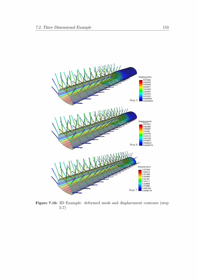
7.2. Three Dimensional Example 153
Step 5
Step 6
Step 7
Figure 7.16: 3D Example: deformed mesh and displacement contours (step5-7)

154 7. Examples

155
Chapter 8
Conclusions
The overall aim was the development of a new numerical simulation tool
(BEFE++) which is especially capable to simulate conventional tunnelling
problems. The ambition was to create a more user-friendly, efficient and accu-
rate program than commonly used programs.
For this the Boundary Element Method (BEM) was chosen. Since the Boundary
Element Method (BEM) is the only method which does not require domain
discretisation, the mesh is much smaller and simpler. Thus the mesh generation
is more user-friendly, the calculation time is shorter and the mesh is less error-
prone. The effort to do 3D simulations is significantly reduced. Additional
advantages are the better accuracy of stress/strain results and the accurate
computability of stress concentration problems.
Since the BEM is not as far developed as other methods a lot of research
and developing work had to be done. All necessary features for simulating
conventional tunnelling processes (for example: sequential excavation, nonlinear
material behaviour, installation of ground supports) had to be developed and
implemented into this new program.
The goal of this work was the development and the implementation of approaches
to simulate ground support (like rock bolts and pipe roofs) into BEFE++. Novel
methods were developed to simulate these inclusions. In the previous chapters

156 8. Conclusions
the simulation of different kinds of rock bolts, pipe umbrella systems and
geological inhomogeneities were presented.
In these methods the inclusions are simulated by applying stresses or forces to
the system. An iterative solution procedure was proposed for these calculations.
With this, a huge number of inclusions (for example rock bolts) can be calculated
efficiently and the iterative procedure can be easily and efficiently combined with
a non-linear calculation (for example to simulate plastic material behaviour). It
was also shown that these procedures work very well in combination with the
coupling algorithm of multiple regions.
In contrast to commonly used methods the mesh generation for such problems
is very easy and independent from any domain discretisation. With a relative
small effort very accurate results are obtained.
Especially the simulation of rock bolts and anchors has key benefits compared to
other methods. Whereas other methods (like the Finite Element Method) needs
an extremely fine mesh around the bolts to handle the local stress concentrations,
the capability of the BEM to deal with stress concentration problems is utilised
and makes the BEM more efficient and more accurate for this kind of problems,
see chapter 5 and chapter 6.
At the end of the chapters small examples were presented to verify each method
separately. Finally some larger examples were shown in which the different
inclusions and also plastic material behaviour were demonstrated to work
together.

157
Bibliography
Aliabadi, M. and Saleh, A. (2002). Fracture mechanics analysis of cracking inplain and reinforced concrete using the boundary element mehtod. Engeneer-ing Fracture Mechanics, 69, 267 – 280.
Banerjee, P. (1981). The Boundary Element Methods in Engineering. McGRAW-HILL Book Company Europe.
Beer, G. (2001). Programming the Boundary Element Method. JHON WILEY& SONS, LTD.
Beer, G., Smith, I., and Duenser, C. (2008). The Boundary Element Methodwith Programming. Springer WienNewYork.
Beer, G. and Watson, J. (1994). Introduction to Finite and Boundary ElementMethods for Engineers. JOHN WILEY & SONS.
Benmokrane, B., Chennouf, A., and Mitri, H. (1995). Loboratory evaluation ofcement-based grouted rock anchors. Int. J. Rock Mech. Min. Sci. & Geomech.Abstr., 32, 633 – 642.
Brebbia, C., Telles, C., and Wrobel, L. (1984). Boundary Element Techniques.Springer, Heidelberg.
Chen, S.-H., Qiang, S., Chen, S.-F., and Egger, P. (2004). Composite elementmodel of the fully grouted rock bolts. Rock Mechanics and Rock Engineering,37, 193 – 212.
Cisilino, A. and Aliabadi, M. (1998). A boundary element method for three-dimensional elastoplastic problems. Engineering Computations, 15, 1011 –1030.
Coda, H. (2001). Dynamic and static non-linear analysis of reinforced media: abem/fem coupling approach. Computers and Structures, 79, 2751 – 2765.
Coda, H. and Venturini, W. (1999). On the coupling of 3d bem and fem framemodel applied to elastodynamic analysis. International Journal of Solids andSturctures, 36, 4789 – 4804.

158 Bibliography
Duenser, C. (2001). Simulation of Sequential Tunnel Excavation with theBoundary Element Method. PhD thesis, Graz University of Technology,Austria.
Feder, G. and Arwanitakis, M. (1976). Zur gebirgsmechanik ausbruchnaher bere-iche tiefliegender hohlraumbauten. Berg- und Huttenmannische Monatshefte,4, 102 – 117.
Filho, R., Mendonca, A., and Paiva, J. (2005). Static boundary element analysisof piles submitted to horizontal and vertical loads. Engineering Analysis withBoundary Elements, 29, 195 – 203.
Gakkov, F. (1966). Boundary Value Problems. Pergamon Press Ltd.
Galler, R. (2009). The new guidline - natm - the austrian way of conventionaltunnelling. In ITA-AITES World Tunnel Congress 2009 - Safe Tunnellingfor the City and for the Environment.
Gao, X. and Davies, T. (2002). Boundary Element Programming in Mechanics.Cambridge University Press.
Gaul, L., Kogl, M., and Wagner, M. (2003). Boundary Element Methods forEngineers and Scientists. Springer-Verlag.
Gioda, G. and Swoboda, G. (1999). Developments and applications of thenumerical analysis of tunnels in continuous media. Internaltional journal fornumerical and analytical methods in geomechanics, 23, 1393–1405.
Guiggiani, M. and Casalini, P. (1987). Direct computuation of cauchy principalvalue integrals in advanced boundary elements. Internaltional Journal forNumerical Methods in Engineering, 24, 1711 – 1720.
Guiggiani, M. and Gigante, A. (1990). A general algorithm for multidimensionalcauchy principal value integrals in the boundary element method. Journal ofApplied Mechanics, 57, 906 – 915.
Hagen, C. (2005). Wechselwirkungen zwischen Bauwerk, Boden und Fluid untertransienter Belastung. PhD thesis, Technische Universitat Hamburg-Harburg.
Hoek, E., Kaiser, P., and Bawden, W. (1997). Support of Underground Excava-tions in Hard Rock. A.A.Balkema Publishers.
Hyett, A., Moosavi, M., and Bawden, W. (1996). Load distribution alongfully grouted bolts, with emphasis on cable bolt reinforcement. InternationalJournal for numerical and analytical Methods in Geomechanics, 20, 517 – 544.
Ivanovic, A. and Neilson, R. D. (2009). Modelling of debinding along the fixedanchor length. International Journal of Rock Mechanics and Mining Sciences,46, 699 – 707.

Bibliography 159
Jing, L. (2003). A review of techniques, advances and outstanding issues innumerical modelling for rock mechanics and rock engineering. Rock Mechanicsand Mining Sciences, 40, 283 – 353.
Jing, L. and Hudson, J. (2002). Numerical methods in rock mechanics. Interna-tional Journal of Rock Mechanics and Mining Sciences, 39, 409 – 427.
Karakus, M. and Fowell, R. (2004). An insight into the new austrian tunnellingmethod (natm). In ROCKMEC 2004 - VIIth Regional Rock MechanicsSymposium.
Kovari, K. (2003a). History of the sprayed concrete lining method - part i:milestones up to the 1960s. Tunnelling and Underground Space Technology,18, 57 – 69.
Kovari, K. (2003b). History of the sprayed concrete lining method - part ii:milestones up to the 1960s. Tunneling and Underground Space Technology,18, 71–83.
Lachat, J. and Watson, J. (1976). Effective numerical treatment of bound-ary integral equations: A formulation for three dimensional elastostatics.International Journal for Numerical Methods in Engineering, 10, 991–1005.
Leite, L., Coda, H., and Venturini, W. (2003). Two-dimensional solids reinforcedby thin bars using the boundary element method. Engineering Analysis withBoundary Elements, 27, 193 – 201.
Leite, L. and Venturini, W. (2005). Boundary element formulation for 2d solidswith stiff and soft inclusions. Engineering Analysis with Boundary Elements,29, 257 – 267.
Ma, F., Chatterjee, J., Henry, D., and Banerjee, P. (2008). Transient heatconduction analysis of 3d solids with fiber inclusions using the boundaryelement method. International Journal for Numerical Methods in Engineering,73, 1113 – 1136.
Maeso, O., Aznarez, J., and Garcia, F. (2005). Dynamic impedances of pile andgroups of piles in saturated soils. Computers and Structures, 83, 769 – 782.
Marence, M. (1992). Numerical Model for Rockbolts under Consideration ofRock Joint Movements. PhD thesis, University of Insbruck.
Mikhilin, S. and Prossdorf, S. (1987). Singular Integral Operators. Springer-Verlag.
Padron, L., Anarez, J., and Maeso, O. (2007). Bem-fem coupling model forthe dynamic analysis of piles and pille groups. Engineering Analysis withBoundary Elements, 31, 473 – 484.

160 Bibliography
Pande, G., Beer, G., and Williams, J.-R. (1990). Numerical Methods in RockMechanics. John Wiley & Soms Ltd.
Paris, F. and Canas, J. (1997). Boundary Element Method - Fundamentals andApplications. Oxford University Press.
Pereira, A. (2008). Coupling BEM/FEM for fluid-soil-structure interaction.PhD thesis, Graz University of Technology, Austria.
Prazeres, P. G. C. (2009). Nonlinear Analysis of NATM Tunnel construction withthe Boundary Element Method. PhD thesis, Graz University of Technology,Austria.
Press, W., Teukolsky, S., Vetterling, W., and Flannery, B. (2002). NumericalRecipes in C++, The Art of Scientific Computing (Second Edition ed.).Cambridge University Press.
Ribeiro, T. (2006). Elastoplastic boundary element method with adaptive cellgeneration. PhD thesis, Graz University of Technology, Austria.
Ribeiro, T., Beer, G., and Duenser, C. (2008). Efficient elastoplastic analysiswith the boundary element method. Computational Mechanics, 41 (5), 715–732.
Riederer, K. and Beer, G. (2009). Boundary element analysis of rock boltsand pipe roofs in tunnels. In Computational Methods in Tunneling, pages115–122.
Riederer, K., Duenser, C., and Beer, G. (2009). Simulation of linear inclusionswith the BEM. Engineering Analysis with Boundary Elements, 33, 959–965.
Romana, M. (2009). Could the new austrian tunnelling method beused safely in cities? In ITA-AITES World Tunnel Congress2009 - Safe Tunnelling for the City and for the Environment,(www.stmr.es/recursos/downloads/AustrianTunnelingMethod.pdf).
Schubert, W. (1997). Grundlagen der New Austrian Tunnelling Method. LectureNotes, Institute for Rock Mechanics and Tunnelling, Graz University ofTechnology, Austria.
Schweiger, H. F. (2008). Computational Geotechnics. Lecture Notes WS 08/09,Institute for Soil Mechanics, Graz University of Technology, Austria.
Telles, J. (1983). The Boundary Element Method Applied to Inelastic Prolems.Springer-Verlag.
Thoeni, K. (2009). Error-Controlled Adaptive Analysis of Non-Linear Prob-lems using the Boundary Element Method. PhD thesis, Graz University ofTechnology, Austria.

Bibliography 161
Venturini, W. S. (1983). Boundary Element Method in Geomechanics. Springer-Verlag.
Wang, Y. and Gao, X. (1998). Practicable bem analysis of frictional bolts inunderground opening. Journal of Structural Engineering, 124, 342 – 346.
Wikipedia. www.wikipedia.com; free encyclopedia.
Zienkiewicz, O., Kelly, D., and Bettess, P. (May 1977). Marriage a la mode- the best of both worlds. Int. Symp. on Innovative Numerical Analysis inApplied Engineering Science, Versailles, France.

162 Bibliography

163
List of Figures
2.1 Configurations involved in Betti’s theorem . . . . . . . . . . . . 252.2 Unit point load b∗i in the domain V ∗ . . . . . . . . . . . . . . . . 282.3 Spherical boundary extension around the load point Q . . . . . 322.4 Problem considering forces b, initial stresses σ0, initial strains ε0 372.5 Problem considering a concentrated point forces bp and a line-
loading bl . . . . . . . . . . . . . . . . . . . . . . . . . . . . . . 392.6 Introducing a modified volume Vε . . . . . . . . . . . . . . . . . 422.7 Boundary discretisation in 2D with quadratic elements . . . . . 472.8 Quadratic shape functions for a 1D element . . . . . . . . . . . 482.9 Quadratic quadrilateral element, intrinsic coordinates ξ and η
and local nodes n = 1...8 . . . . . . . . . . . . . . . . . . . . . . 492.10 Domain discretised with integration cells V c . . . . . . . . . . . 502.11 Quadratic brick cells, intrinsic coordinates ξ, η, ζ and local nodes
n = 1...20 . . . . . . . . . . . . . . . . . . . . . . . . . . . . . . 512.12 Weak singularity: integrand f (x) and integral I (x) . . . . . . . 612.13 Strong singularity: integrand f (x) and integral I (x) . . . . . . 62
3.1 Methods to simulate inhomogeneous domains . . . . . . . . . . 673.2 Simulation of embedded inclusions with initial stresses . . . . . 683.3 Flow chart of the iterative algorithm . . . . . . . . . . . . . . . 753.4 Flow chart of the iterative algorithm for coupled problems . . . 763.5 BE discretisation including different cells . . . . . . . . . . . . . 77
4.1 Geological inclusion discretised with cells . . . . . . . . . . . . . 804.2 Grouted pipe roofing technique . . . . . . . . . . . . . . . . . . 804.3 Approximated modelling of pipe roofs . . . . . . . . . . . . . . . 814.4 Schematic diagram for computing the residuum for soft and hard
inclusions . . . . . . . . . . . . . . . . . . . . . . . . . . . . . . 864.5 Schematic figure of the stress states for inclusions with nonlinear
material behaviour . . . . . . . . . . . . . . . . . . . . . . . . . 874.6 Example 1: vertical displacements on the top of the block . . . . 904.7 Example 1: deformed mesh and contours of vertical displacements 904.8 Example 2: deformed mesh and contours of vertical displacements 91

164 List of Figures
4.9 Example 2: vertical displacements along the top of the block . . 924.10 Example 2: vertical displacements along the top of the inclusion 924.11 Example 3: deformed shape and displacement contours . . . . . 934.12 Example 3: deformed shape and contours of vertical stresses . . 944.13 Example 4: deformed mesh after the second calculation step . . 954.14 Example 4: vertical displacements along the top of the cantilever 95
5.1 Different types of continuous anchored bolts, see Hoek et al. (1997) 985.2 Line-cells with three nodes and quadratic interpolation . . . . . 1025.3 Local coordinate system of a bolt in 3D . . . . . . . . . . . . . . 1045.4 Schematic illustration of the stresses in the rock, in the bolt and
the initial stresses (σRockxx , σBoltxx and σ0 xx). . . . . . . . . . . . . 1075.5 Computation of residual stresses by bolt-yielding . . . . . . . . 1095.6 Equilibrium on a small part of the bolt . . . . . . . . . . . . . . 1105.7 Singular integration over the line-cell . . . . . . . . . . . . . . . 1165.8 Schematic representation of a bolt and it’s stress distribution . . 1195.9 Example 1: vertical displacements along the bolt . . . . . . . . 1205.10 Example 2: vertical displacements along the bolt . . . . . . . . 1215.11 Example 3: effects of variational bond stiffness’s . . . . . . . . . 1225.12 Example 4: effects of variational bolt yield stress . . . . . . . . . 123
6.1 Different types of discrete anchored bolts (see Hoek et al. 1997) 1256.2 Pair of points to model discrete anchored bolts . . . . . . . . . . 1296.3 Modelling of the bonded end of an anchor . . . . . . . . . . . . 1296.4 Replacing the concentrated force by a volume force at the singular
point . . . . . . . . . . . . . . . . . . . . . . . . . . . . . . . . . 1366.5 Example 1: vertical displacements along the bolt . . . . . . . . 1396.6 Example 2: vertical displacements along the bolt . . . . . . . . 140
7.1 Example 1: mesh discretisation . . . . . . . . . . . . . . . . . . 1427.2 Example 1: displacements along the vertical bolt . . . . . . . . 1427.3 Example 1: deformed BE-mesh contour lines . . . . . . . . . . . 1437.4 Example 2: mesh discretisation . . . . . . . . . . . . . . . . . . 1447.5 Example 2: deformed BE-mesh contours of displacements . . . . 1447.6 Example 2: displacements in axial bolt directions . . . . . . . . 1457.7 Example 2: bolt stresses . . . . . . . . . . . . . . . . . . . . . . 1457.8 Example 3: contours of displacements (PL+RB+PU) . . . . . . 1477.9 Example 3: tangential stresses in the rock mass . . . . . . . . . 1477.10 Example 3: displacement-results (tunnel roof and tunnel floor) . 1487.11 3D Example: tunnel geometry and BE-mesh . . . . . . . . . . . 1497.12 3D Example: longitudinal sections . . . . . . . . . . . . . . . . . 150

List of Figures 165
7.13 3D Example: deformations along the tunnel roof (steps 2-7) . . 1517.14 3D Example: comparison of vertical displacements . . . . . . . . 1517.15 3D Example: deformed mesh and displacement contours (step 1-4)1527.16 3D Example: deformed mesh and displacement contours (step 5-7)153

166 List of Figures

167
List of Tables
2.1 Gauss points ξ and weights w for Gauss quadrature . . . . . . . 552.2 Different types of singularities . . . . . . . . . . . . . . . . . . . 56
7.1 3D Example: activities in segments during construction stages . 1507.2 3D Example: comparison of vertical displacements . . . . . . . . 151