UPTEC W 14020

Examensarbete 30 hpJuni 2014

Modelling of algae based wastewater treatment Implementation of the River Water Quality

Model no. 1

Rasmus Pierong

ABSTRACT

Modelling of algae based wastewater treatment – Implementation of the River Water Quality Model no. 1

Rasmus Pierong

The conventional wastewater treatment of today was developed aiming to mitigate problems occurring in wastewater recipients such as oxygen depletion and eutrophication. The focus of wastewater management has however broadened and major concern is now focused on the sustainability of the wastewater treatment process itself. Algae based wastewater treatment is an alternative to conventional treatment. It has the potential to yield an acceptable effluent quality at a lower ecological cost.

This Degree Project was conducted as part of MOBIT, a project at Mälardalen University. The MOBIT project was aimed at the development of an algae based wastewater treatment process in an activated sludge environment. The aim of this Degree Project was to propose a model describing the dynamics of such a system. The model was constructed in Simulink, based on the River Water Quality Model no. 1. The River Water Quality Model no. 1 was chosen as the basis for modelling because it included the state variables and processes necessary to describe the dynamics of bacteria, algae and pH.

The River Water Quality Model no. 1 was, as the name suggests, developed to describe a river system. It was hence considered important to evaluate if the model was applicable to an activated sludge environment. A major obstacle was the fact that no algae based activated sludge system had been studied prior the start of the MOBIT project, the project was pioneering. The lack of system understanding and of measurement data aggravated the evaluation. However, the proposed model was compared to the Activated Sludge Model No. 1 which was known to describe an activated sludge system accurately.

The model structure of the River Water Quality Model no. 1 was considered a good starting point for future modelling of the algae based activated sludge process. However, the model set-up proposed in this report does not describe the system sufficiently well. Better system understanding and measurement data is needed in order to develop and calibrate the model.

Keywords: algae, wastewater treatment, activated sludge process, modelling, RWQM1, ASM1.

Department of Information Technology, Uppsala UniversityBox 337SE-751 05 UppsalaISSN: 1401-5765, UPTEC W 14 020

i

REFERAT

Modellering av algbaserad avloppsvattenrening – Implementering av River Water Quality Model no. 1

Rasmus Pierong

Dagens konventionella avloppsvattenrening har utvecklats för att minimera utsläpp av näringsämnen och kolföreningar då sådana utsläpp medför övergödning och syrebrist i mottagande vatten. På senare tid har reningsprocessen i sig hamnat i fokus då den är såväl energi- som resurskrävande. Algbaserad avloppsvattenrening är ett alternativ som har potential att ge tillfredsställande rening med ett betydligt mindre ekologiskt fotavtryck.

Det här examensarbetet var en del av MOBIT, ett projekt vid Mälardalens högskola. MOBIT syftade till att utvärdera algbaserad avloppsvattenrening i form av en aktivslamprocess. Syftet med examensarbetet var att ta fram en modell för det planerade systemet. Modellen byggdes i Simulink och den baserades på en befintlig modell, River Water Quality Model no. 1. Den befintliga modellen valdes för att den inkluderade alla önskvärda tillståndsvariabler och processer, bland annat de som krävs för att beskriva alg-, bakterie- och pH-dynamik.

Som namnet antyder utvecklades River Water Quality Model no. 1 för att beskriva ett flodsystem. Det var därför angeläget att utvärdera huruvida modellen var tillämpbar i en aktivslammiljö. Utvärderingen försvårades av att det vid tiden för examensarbetets utförande ännu inte fanns någon existerande algbaserad aktivslamprocess. Kunskapen om systemet var därför begränsad och det fanns ingen mätdata att kalibrera eller evaluera mot. I brist på mätdata jämfördes den framtagna modellen med en annan modell som var utvecklad för att beskriva just avloppsvattenrening, Activated Sludge Model No. 1.

Arbetet resulterade i slutsatsen att River Water Quality Model no. 1 utgör en bra grund för modellering av den algbaserade aktivslamprocessen. Men, den modellkonfiguration som tas fram i denna rapport beskriver inte systemet särskilt bra. Bättre systemförståelse samt tillförlitlig mätdata krävs för att omarbeta och kalibrera den föreslagna modellen.

Nyckelord: alger, avloppsvattenrening, aktivslamprocessen, modellering, RWQM1, ASM1.

Institutionen för informationsteknologi, Uppsala universitetBox 337SE-751 05 UppsalaISSN: 1401-5765, UPTEC W 14 020

ii

PREFACE

This thesis was conducted as part of MOBIT, a project at Mälardalen University. I had two supervisors, Emma Nehrenheim and Carl-Fredrik Lindberg. Both of them were engaged in MOBIT. Emma is Senior Lecturer in Environmental Engineering and Carl-Fredrik is Adjunct Professor of Process Automation with focus on Energy Efficiency. Bengt Carlsson was my subject reader. He is Professor in Automatic Control at the Department of Information Technology, Uppsala University.

I want to thank my subject reader and my two supervisors for their engagement in this thesis. I would also like to wish my two supervisors and the rest of the MOBIT group good luck with their future work on algae based wastewater treatment. I am looking forward to a future full of fertilizer producing, carbon dioxide capturing and sustainable algae based wastewater treatment plants.

This thesis marks the end of my studies at the Master's Programme in Environmental and Water Engineering at Uppsala University, which I initiated in 2008. It has been a wonderful time.

Rasmus PierongUppsala, 2014

Copyright © Rasmus Pierong and the Department of Information Technology, Uppsala UniversityUPTEC W 14 020, ISSN: 1401-5765Digitally published at the Department of Earth Sciences, Uppsala University, Uppsala, 2014.

iii

POPULÄRVETENSKAPLIG SAMMANFATTNING

Modellering av algbaserad avloppsvattenrening – Implementering av River Water Quality Model no. 1

Rasmus Pierong

Dagens konventionella avloppsvattenrening har utvecklats för att minimera effekterna av de problem som avloppsvatten ger upphov till i mottagande ekosystem. Reningsverken har utvecklats i takt med att nya problem har uppmärksammats. På trettiotalet byggdes sedimentationsanläggningar och mekaniska hinder för att minska utsläppen av synliga föroreningar. Tjugo år senare kopplades det växande problemet med syrefria bottnar samman med utsläpp av organiskt material. För att minska utsläppen infördes biologisk rening, den så kallade aktivslamprocessen. Aktivslamprocessen bygger på att den bakteriekultur som naturligt finns i avloppsvatten gynnas genom att vattnet får passera en syresatt bassäng och en sedimentationsanläggning i vilken bakterierna faller till botten för att sedan återföras till den syresatta bassängen. På så sätt upprätthålls en hög bakteriekoncentration i en syrerik miljö där bakterierna aktivt bryter ner organiskt material. Trots att aktivslamprocessen medförde lägre utsläpp av organiskt material så återstod ofta problemen med syrefria bottnar. Orsaken var de växande fosforutsläppen. På sjuttiotalet började man därför fälla ut fosfor med hjälp av fällningskemikalier så som aluminiumsulfat och järnsulfat. Den sista större förändringen av svensk avloppsvattenrening genomfördes på nittiotalet för att minska kväveutsläppen då kväve bidrar till övergödning i delar av Östersjön och i större hav. Kväverening utförs vanligen genom nitrifikation och denitrifikation, två processer som tillsammans gör att kvävet omvandlas till gasform och går ut i atmosfären. På senare tid har fokus riktats mot själva reningsprocessen och de nackdelar som konventionell avloppsvattenrening medför. Mycket energi går åt då avloppsvattnet syresätts och det kväve som renas bort från avloppsvattnet släpps ut i atmosfären istället för att omhändertas och användas som gödsel. Algbaserad avloppsvattenrening utgör ett alternativ till den konventionella avloppsvattenreningen. Ett alternativ som kan ge önskad reningsgrad till ett mindre ekologiskt fotavtryck. Tanken är att algerna ska producera syre vilket minskar behovet av mekanisk syresättning. Dessutom ska deras stora näringsupptag ersätta den konventionella kvävereningen. På så sätt kan kvävet tillvaratas som gödsel.

Det här examensarbetet var en del av MOBIT, ett projekt vid Mälardalens högskola. Syftet med MOBIT var att utvärdera en algbaserad aktivslamprocess och i projektet ingick bland annat uppförandet av en pilotanläggning. Syftet med examensarbetet var att ta fram en modell för den planerade aktivslamprocessen. Modellen skulle beskriva hur pH-värdet och koncentrationen av bland annat alger, bakterier och näringsämnen varierar i systemet, och den skulle ligga till grund för vidare utveckling inom MOBIT. Den modell som togs fram baserades på en existerande modell vid namn River Water Quality Model no. 1. Denna var egentligen framtagen för att beskriva ett flodsystem men den innehöll samtliga komponenter som ansågs nödvändiga för att beskriva en algbaserad aktivslamprocess och utgjorde därmed en bra grund.

En viktig del av examensarbetet var att utvärdera den framtagna modellen. Utvärderingen försvårades av att det då examensarbetet genomfördes inte fanns någon pilotanläggning att ta mätdata ifrån eller att studera för ökad systemförståelse. I brist på mätdata utvärderades modellen genom jämförelser med en annan, inom den konventionella avloppsvattenreningen väl använd och accepterad, modell. Resultatet av examensarbetet visade att den framtagna modellen utgör en bra grund för fortsatt modellering men att bättre systemförståelse och bättre tillgång till mätdata krävs för vidare utveckling och kalibrering.

iv

Table of Contents 1 Introduction............................................................................................................................................1

1.1 Aim of study....................................................................................................................................22 Theory.....................................................................................................................................................3

2.1 Modelling of wastewater treatment systems...................................................................................32.1.1 State variables and their derivatives........................................................................................32.1.2 The activated sludge process...................................................................................................4

2.2 Modelling of algae dynamics..........................................................................................................52.2.1 Factors limiting algal growth...................................................................................................52.2.2 Examples of models describing algal growth..........................................................................72.2.3 Processes reducing the concentration of algae......................................................................102.2.4 Summary of kinetic parameters ............................................................................................11

2.3 Gas exchange ................................................................................................................................113 Simulation models.................................................................................................................................15

3.1 The Activated Sludge Model No. 1...............................................................................................153.2 The Benchmark Simulation Model no. 1......................................................................................163.3 The River Water Quality Model no. 1...........................................................................................17

4 Simulink implementation of the Activated Sludge Model No. 1..........................................................214.1 Implementation and evaluation of the differential equations that define the Activated Sludge Model No. 1..............................................................................214.2 Implementation and evaluation of an activated sludge model based on the Activated Sludge Model No. 1.................................................................................22

5 Simulink implementation of the River Water Quality Model no. 1......................................................245.1 Implementation of the differential equations that define the River Water Quality Model no. 1..................................................................................................245.2 Model set-up, parameter values and influent data selection.........................................................275.3 Evaluation of the activated sludge model based on the River Water Quality Model no. 1..................................................................................................30

5.3.1 Model configurations.............................................................................................................315.3.2 Evaluation results...................................................................................................................32

6 Adapting the activated sludge model based on the River Water Quality Model no. 1 to a wastewater treatment environment...............................................................35

6.1 Hydrolysis.....................................................................................................................................356.2 System identification – the least squares method..........................................................................36

6.2.1 Regression models.................................................................................................................376.2.2 Assumptions done to allow usage of the least squares method with simulation data from the ASM1 set-up.............................................................436.2.3 Parameter approximations.....................................................................................................466.2.4 Evaluation of assumptions.....................................................................................................49

6.3 System identification – non-linear programming..........................................................................497 Introducing algae dynamics..................................................................................................................53

7.1 Development of processes describing algal growth......................................................................537.2 Incorporation of algae dynamics into the activated sludge model based on the River Water Quality Model no. 1..................................................................54

8 Operation strategy analysis...................................................................................................................569 Alternative sedimentation configuration...............................................................................................59

v

10 Discussion...........................................................................................................................................6010.1 Effluent quality and consumers...................................................................................................6010.2 Model structure............................................................................................................................6010.3 Light intensity..............................................................................................................................6010.4 Calibration...................................................................................................................................6010.5 Further research...........................................................................................................................6110.6 Related research..........................................................................................................................62

11 Conclusions.........................................................................................................................................6312 References...........................................................................................................................................64 Appendix A – Gujer matrix summarizing the Activated Sludge Model No. 1.....................................................................................................................67 Appendix B – Gujer matrix summarizing the River Water Quality Model no. 1......................................................................................................................68 Appendix C – Stoichiometric coefficients used in applications of the River Water Quality Model no. 1...............................................................................69 Appendix D – Process rates of the River Water Quality Model no. 1.....................................................70 Appendix E – S-function describing the differential equations of the River Water Quality Model no. 1.....................................................................................72

vi

1 INTRODUCTION

Wastewater treatment is an important part of modern society and a prerequisite for a sustainable water usage. The role of wastewater treatment has continuously changed. Identification of new problems arising from wastewater pollution has changed the focus of the treatment process, increasing the complexity of treatment plants. The origin of western wastewater treatment has been attributed to Joseph Bazalgette in the middle of the nineteenth century (Chapra, 2011). He was the chief engineer of an extensive expansion of London's sewage system, a measure taken to tackle the huge sanitation problem referred to as “The Great Stink of 1858”.

The development of Swedish wastewater treatment from the time of Bazalgette until today may be summarized in four consequent landmarks in terms of treatment adaptations. These adaptations have been presented by Bernes and Lundgren (2009) and the remaining part of this text section is based on their work. Mechanical treatment was introduced in the 1930s in order to solve problems with visible litter. In the 1950s, problems with oxygen depletion caused by high organic loads were mitigated by the introduction of the biological wastewater treatment known as the activated sludge process. However, it was soon found that problems with oxygen depletion often remained after the introduction of biological treatment. This was due to the emergence of extensive algal blooms coupled to oxygen consuming decay processes. The algal blooms were caused by the increasing phosphorous eutrophication. Chemical precipitation, for example iron sulphate or aluminium sulphate, was introduced in the 1970s in order to reduce the phosphorous concentration of the treated wastewater. This measure was found to function well in that the phosphorous concentration of many recipients decreased, as did the extent of algal blooms. The last major adaptation of Swedish wastewater treatment was the introduction of nitrogen removal. It was done in the 1990s aiming for mitigation of the nitrogen eutrophication occurring in the Baltic Sea and in larger oceans.

All adaptations described above was conducted to improve the water quality of wastewater recipients. The focus of wastewater treatment management has however broadened. Major concern is now focused on the sustainability of the wastewater treatment process itself. Conventional wastewater treatment has several drawbacks such as the extensive usage of precipitation chemicals, energy and external carbon. Energy is consumed in the activated sludge process while external carbon is used in the process of nitrogen removal. Nitrogen is removed through nitrification and denitrification. These processes are thoroughly described in literature, for example by Svenskt Vatten (2010). The activated sludge process requires an aerobic environment which is obtained through energy intensive aeration (Svenskt Vatten, 2010). The process of denitrification requires suspended carbon which can be provided through the injection of external carbon (Svenskt Vatten, 2010). However, the usage of external carbon depends upon the configuration of the wastewater treatment plant. Some configurations do not require injection of external carbon while other do. Another major drawback with conventional wastewater treatment is the loss of potentially valuable nutrients (Noüe, Laliberté and Proulx, 1992). Nitrogen is emitted to the atmosphere through the processes of nitrification and denitrification.

Algae based wastewater treatment is an alternative to conventional wastewater treatment. The method has been investigated for more than 50 years, it is well documented and overviews have been provided by Hoffmann (1998) and Noüe, Laliberté and Proulx (1992). Algae based wastewater treatment has the potential to circumvent several of the problems encountered in conventional wastewater treatment. The oxygen that is produced during algal photosynthesis reduces the need for energy intensive aeration. It might even make the aeration redundant. Carbon dioxide is consumed during photosynthesis. Hence, an algae based wastewater treatment plant may potentially work as a carbon dioxide sink mitigating global

1

warming. It has been shown that algae based wastewater treatment is sufficient for high level reductions of organic matter, nitrogen and phosphorous, as discussed by Hoffmann (1998). The large nutrient uptake of algae may replace the usage of chemical precipitation and the processes of nitrification and denitrification. This would make the extensive usage of precipitation chemicals and external carbon redundant. Also, the sludge produced in an algae base wastewater treatment process would be rich in both nitrogen and phosphorous, and hence a potentially valuable fertilizer.

This study was conducted as part of MOBIT, a project at Mälardalen University. The MOBIT project was aimed at the development of an algae based wastewater treatment process in an activated sludge environment. This type of algae based wastewater treatment configuration had not been investigated before and the MOBIT project was hence pioneering.

1.1 AIM OF STUDY

The overall aim of this thesis was to propose a model describing the dynamics of an algae based wastewater treatment process in an activated sludge environment. The model was to form the basis for future modelling aimed at control and operation strategy analyses within the MOBIT project.

The model was supposed to include pH dynamics. It was also supposed to be based on an existing and acknowledged model, preferably the Activated Sludge Model No. 1 (ASM1) as presented in section 3.1. However, pH dynamics are complex. They are governed by several processes such as the chemical equilibria of, inter alia, carbon dioxide-bicarbonate, bicarbonate-carbon trioxide, and ammonium-ammonia. A model must hence be relatively large in order to describe pH dynamics accurately. ASM1 only includes a fraction of the state variables necessary for estimating the pH value. It was hence considered infeasible to use that model as a starting point for the model development of this study.

The River Water Quality Model no. 1 (RWQM1), presented in section 3.3, includes all state variables and processes needed to describe both pH dynamics and algae dynamics. It was hence considered to be a feasible starting point for the model development of this study. However, it should be emphasized that RWQM1 was developed to describe the dynamics of a river system and not an activated sludge process.

The overall aim was condensed to the implementation of an algae based activated sludge model in Simulink, based on RWQM1. It was considered important to investigate how well this model set-up mimicked the system dynamics of an activated sludge process, given the fact that it was developed to describe a river system. The bacterial dynamics of the proposed model set-up was to be compared to the bacterial dynamics of ASM1. The proposed model set-up was also to be adjusted and calibrated in order to increase the consistency with ASM1.

2

2 THEORY

2.1 MODELLING OF WASTEWATER TREATMENT SYSTEMS

2.1.1 State variables and their derivatives

The core of a wastewater treatment model consists of a set of state variables, one for each component that is to be modelled. A state variable may for example represent the concentration of bacteria, the concentration of biodegradable substrate or the concentration of dissolved oxygen. The number of state variables included in a specific model varies depending on the application domain of that model. Examples of state variables are found in Table 4 and Table 6.

Wastewater treatment models are used to describe system dynamics in terms of the change of state variables. They must hence include routines for the calculation of state variable derivatives. These routines differ depending on application domain. The derivatives of a model describing the dynamics of an isolated water basin will depend upon biochemical processes alone. The derivatives of a model describing the dynamics of a water basin subject to in- and outflow will depend upon both biochemical processes and mass transports.

Mass transports are calculated according to

dSdt

=S in⋅Qin

V−

S⋅Qout

V=

QV

⋅(S in−S ) (1)

with S as the concentration of the subject state variable, Q as the flow magnitude, index in denoting the inflow, index out denoting the outflow and V denoting the basin volume. The inflow magnitude is assumed to equal the outflow magnitude.

Biochemical processes appear in many different forms. State variables representing living organisms such as bacteria, algae or zoo-plankton are often described as governed by the processes of growth, death, respiration, grazing and predation. The growth process is usually represented as a specific growth rate multiplied by the concentration of the subject state variable according to

dSdt

= μ⋅S. (2)

The specific growth rate is usually defined as a function of the maximal specific growth rate μmax and several factors limiting growth according to

μ = μmax⋅∏i=1

N

f ( si) (3)

with N as the total number of limiting factors and f(si) defining to what extent factor si limits growth. Light intensity and temperature are examples of limiting factors. The concentration of biodegradable matter, inorganic phosphorous, inorganic nitrogen and dissolved oxygen are other examples. The function that defines how much a limiting factor affects the growth rate can take many different forms.

A commonly used function is the Monod function. It is defined as

f (si) =si

K s+s i(4)

3

with si as the value of the limiting factor and KS as the half saturation coefficient. Some other functions are presented in sub-section 2.2.1.

2.1.2 The activated sludge process

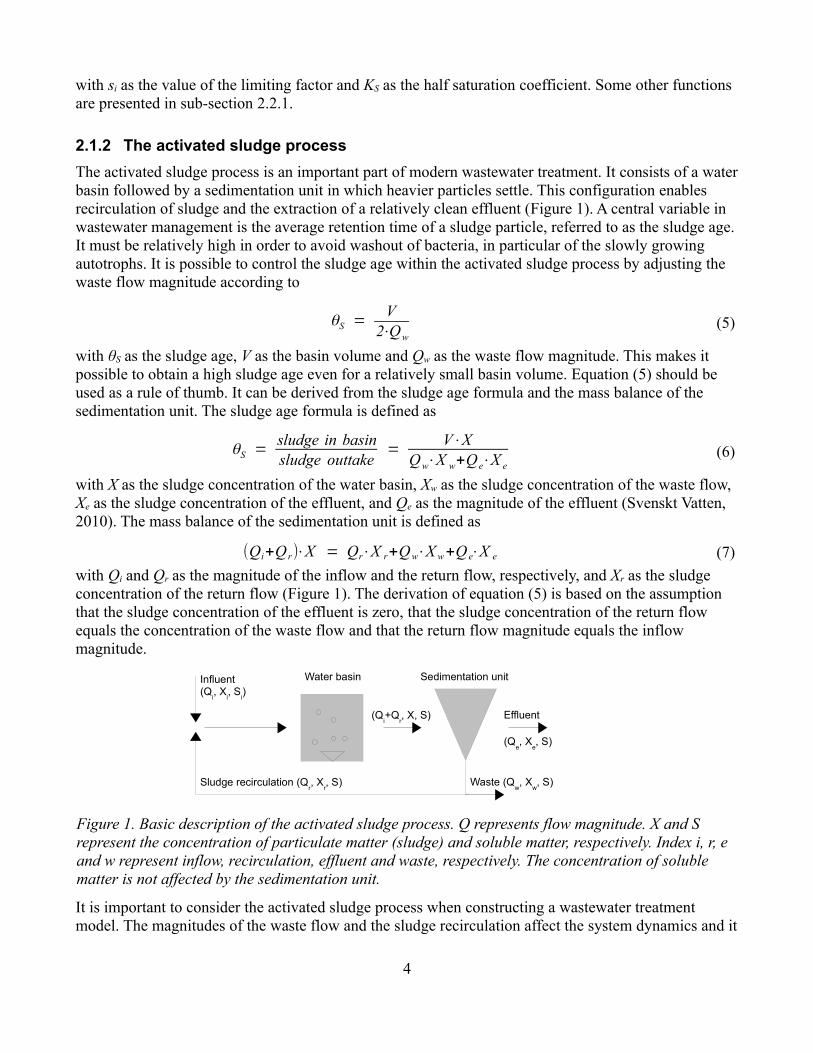
The activated sludge process is an important part of modern wastewater treatment. It consists of a water basin followed by a sedimentation unit in which heavier particles settle. This configuration enables recirculation of sludge and the extraction of a relatively clean effluent (Figure 1). A central variable in wastewater management is the average retention time of a sludge particle, referred to as the sludge age. It must be relatively high in order to avoid washout of bacteria, in particular of the slowly growing autotrophs. It is possible to control the sludge age within the activated sludge process by adjusting the waste flow magnitude according to

θS =V

2⋅Qw(5)

with θS as the sludge age, V as the basin volume and Qw as the waste flow magnitude. This makes it possible to obtain a high sludge age even for a relatively small basin volume. Equation (5) should be used as a rule of thumb. It can be derived from the sludge age formula and the mass balance of the sedimentation unit. The sludge age formula is defined as

θS =sludge in basinsludge outtake

=V⋅X

Qw⋅X w+Q e⋅X e(6)

with X as the sludge concentration of the water basin, Xw as the sludge concentration of the waste flow, Xe as the sludge concentration of the effluent, and Qe as the magnitude of the effluent (Svenskt Vatten, 2010). The mass balance of the sedimentation unit is defined as

(Qi+Q r)⋅X = Qr⋅X r+Qw⋅X w+Q e⋅X e (7)

with Qi and Qr as the magnitude of the inflow and the return flow, respectively, and Xr as the sludge concentration of the return flow (Figure 1). The derivation of equation (5) is based on the assumption that the sludge concentration of the effluent is zero, that the sludge concentration of the return flow equals the concentration of the waste flow and that the return flow magnitude equals the inflow magnitude.

It is important to consider the activated sludge process when constructing a wastewater treatment model. The magnitudes of the waste flow and the sludge recirculation affect the system dynamics and it

4

Figure 1. Basic description of the activated sludge process. Q represents flow magnitude. X and S represent the concentration of particulate matter (sludge) and soluble matter, respectively. Index i, r, e and w represent inflow, recirculation, effluent and waste, respectively. The concentration of soluble matter is not affected by the sedimentation unit.

Influent (Q

i, X

i, S

i)

Effluent

Waste (Qw, X

w, S)Sludge recirculation (Q

r, X

r, S)

Sedimentation unitWater basin

(Qi+Q

r, X, S)

(Qe, X

e, S)

is often desirable to include them as model variables. The sedimentation unit may be modelled assuming ideal sedimentation according to which all particulate matter settle. The concentration of soluble matter is then assumed to be the same in all flow lines while the concentration of particulate matter in the return flow and in the waste flow is calculated according to

X r = X w =Qi+Q r

Qr+Qw

⋅X. (8)

Assuming ideal sedimentation is the least complex modelling approach. There are other approaches in which particulate matter may contaminate the effluent, see for example the sedimentation unit implemented within the Benchmark Simulation Model no. 1 (BSM1) as described by Alex et al. (2008b).

2.2 MODELLING OF ALGAE DYNAMICS

Several models describing the dynamics of algae based wastewater treatment systems have been proposed in literature. A literature study was conducted to examine how the algae dynamics of those models were described. The information was considered valuable for the model development of this study.

2.2.1 Factors limiting algal growth

Factors limiting algal growth in one system are not necessarily limiting in an other, as reflected in the models presented in sub-section 2.2.2. It is therefore crucial to consider the application domain of a model when deciding which limiting factors to include in that specific model. Algal growth may be limited by

1. inorganic carbon,

2. nitrogen,

3. phosphorous,

4. light intensity,

5. temperature, and

6. pH.

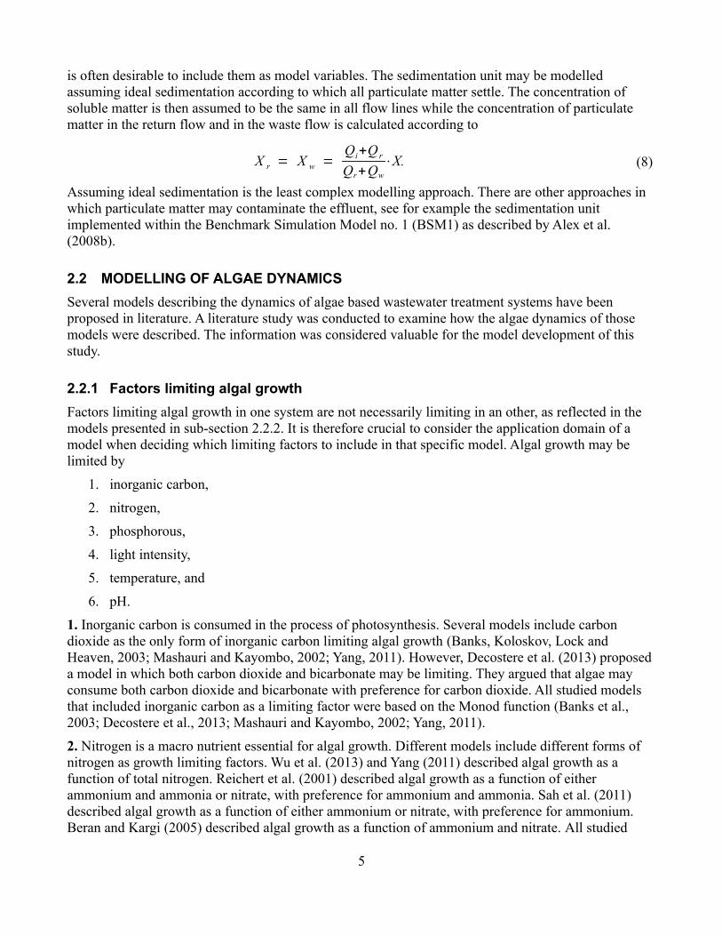
1. Inorganic carbon is consumed in the process of photosynthesis. Several models include carbon dioxide as the only form of inorganic carbon limiting algal growth (Banks, Koloskov, Lock and Heaven, 2003; Mashauri and Kayombo, 2002; Yang, 2011). However, Decostere et al. (2013) proposed a model in which both carbon dioxide and bicarbonate may be limiting. They argued that algae may consume both carbon dioxide and bicarbonate with preference for carbon dioxide. All studied models that included inorganic carbon as a limiting factor were based on the Monod function (Banks et al., 2003; Decostere et al., 2013; Mashauri and Kayombo, 2002; Yang, 2011).

2. Nitrogen is a macro nutrient essential for algal growth. Different models include different forms of nitrogen as growth limiting factors. Wu et al. (2013) and Yang (2011) described algal growth as a function of total nitrogen. Reichert et al. (2001) described algal growth as a function of either ammonium and ammonia or nitrate, with preference for ammonium and ammonia. Sah et al. (2011) described algal growth as a function of either ammonium or nitrate, with preference for ammonium. Beran and Kargi (2005) described algal growth as a function of ammonium and nitrate. All studied

5

models that included nitrogen as a limiting factor were based on the Monod function (Beran and Kargi, 2005; Reichert et al., 2001; Sah et al., 2011; Wu et al., 2013; Yang, 2011).

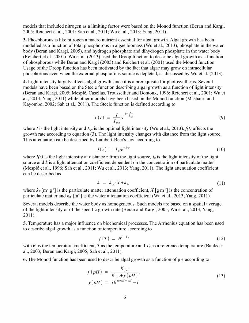
3. Phosphorous is like nitrogen a macro nutrient essential for algal growth. Algal growth has been modelled as a function of total phosphorous in algae biomass (Wu et al., 2013), phosphate in the water body (Beran and Kargi, 2005), and hydrogen phosphate and dihydrogen phosphate in the water body (Reichert et al., 2001). Wu et al. (2013) used the Droop function to describe algal growth as a function of phosphorous while Beran and Kargi (2005) and Reichert et al. (2001) used the Monod function. Usage of the Droop function has been motivated by the fact that algae may grow on intracellular phosphorous even when the external phosphorous source is depleted, as discussed by Wu et al. (2013).

4. Light intensity largely affects algal growth since it is a prerequisite for photosynthesis. Several models have been based on the Steele function describing algal growth as a function of light intensity (Beran and Kargi, 2005; Mesplé, Casellas, Troussellier and Bontoux, 1996; Reichert et al., 2001; Wu et al., 2013; Yang, 2011) while other models have been based on the Monod function (Mashauri and Kayombo, 2002; Sah et al., 2011). The Steele function is defined according to

f (I ) =I

I opt

⋅e1− I

I opt (9)

where I is the light intensity and Iopt is the optimal light intensity (Wu et al., 2013). f(I) affects the growth rate according to equation (3). The light intensity changes with distance from the light source. This attenuation can be described by Lambert-Beer's law according to

I ( z ) = I 0⋅e−k⋅z (10)

where I(z) is the light intensity at distance z from the light source, I0 is the light intensity of the light source and k is a light attenuation coefficient dependent on the concentration of particulate matter (Mesplé et al., 1996; Sah et al., 2011; Wu et al., 2013; Yang, 2011). The light attenuation coefficient can be described as

k = k X⋅X +kW (11)

where kX [m2·g-1] is the particulate matter attenuation coefficient, X [g·m-3] is the concentration of particulate matter and kW [m-1] is the water attenuation coefficient (Wu et al., 2013; Yang, 2011).

Several models describe the water body as homogeneous. Such models are based on a spatial average of the light intensity or of the specific growth rate (Beran and Kargi, 2005; Wu et al., 2013; Yang, 2011).

5. Temperature has a major influence on biochemical processes. The Arrhenius equation has been used to describe algal growth as a function of temperature according to

f (T ) = θT −T 0 (12)

with θ as the temperature coefficient, T as the temperature and T0 as a reference temperature (Banks et al., 2003; Beran and Kargi, 2005; Sah et al., 2011).

6. The Monod function has been used to describe algal growth as a function of pH according to

f ( pH ) =K pH

K pH + y ( pH ),

y ( pH ) = 10∣optpH− pH∣−1

(13)

6

with KpH as the half saturation coefficient and optpH as a parameter defining the optimal pH value (Beran and Kargi, 2005; Mashauri and Kayombo, 2002).

2.2.2 Examples of models describing algal growth

Wu et al. (2013) modelled growth of the algae species Scenedesmus sp. LX1 as a function of total nitrogen using the Monod function, intracellular phosphorous using the Droop function, and light intensity using the Steele function. The model was set up according to

dX A

dt= μmax⋅ f ( I )⋅

S N

K N+S N

⋅(1−Q 0

q p

)⋅X A (14)

with f(I) as the Steele function according to equation (9), XA as the algae concentration, SN and KN as the concentration of total nitrogen and the corresponding saturation coefficient, and qp and Q0 as the phosphorous content in algal biomass and the corresponding minimal content necessary for metabolism. Laboratory experiments were conducted to estimate the different parameter values. The maximal specific growth rate was estimated to 0.79 d-1, the half saturation coefficient for total nitrogen was estimated to 9.5 ± 2.9 g(N)·m-3 and the minimal phosphorous content was estimated to 0.019 ± 0.003 %. They showed that the relationship between algal growth and light intensity was well captured by the Steele model and they suggested that the light intensity of a given depth should be calculated following Lambert-Beer's law according to equation (10).

Decostere et al. (2013) modelled growth of the algae species Chlorella vulgaris as a function of carbon dioxide and bicarbonate with preference for carbon dioxide. The growth process was divided into two sub-processes according to

dX A

dt= μmax⋅

S HCO3

K HCO3+S HCO3

⋅K CO2

KCO2+SCO2

⋅X A ,

dX A

dt= μmax⋅

SCO2

KCO2+S CO2

⋅X A .(15)

The division into sub-processes was necessary in order to relate the change of a specific substrate (carbon dioxide or bicarbonate) to the change of algae concentration. The half saturation parameters KHCO3 and KCO2 were set to 3 g(HCO3)·m-3 and 0.2 g(CO2)·m-3, respectively. Equation (15) was built into a larger model with several state variables such as dissolved oxygen, carbon dioxide and bicarbonate, describing the dynamics of algae in a lab environment. The model was calibrated against experimental data with respect to the maximal specific growth rate and the KLa value (the KLa value is explained in section 2.3). The maximal specific growth rate was thereby estimated to be between 0.48 d-1 and 0.52 d-1. Good model performance indicated reasonable parameter values.

Yang (2011) modelled algal growth as a function of carbon dioxide, total nitrogen and light intensity according to

dX A

dt= μmax⋅ f ( I )⋅

S CO2

KCO2+SCO2

⋅S NH4+S NO3

K NH4+NO3+S NH4+S NO3

⋅X A (16)

with f(I) as defined in equation (9). The maximal specific growth rate was set to 0.9991 d-1 and both half saturation coefficients (KCO2 and KNH4+NO3) were set to 0.001 mol·m-3. The light intensity I was calculated using Lambert-Beer's law according to equation (10). Equation (16) was built into a larger model with several state variables describing the dynamics of algae and bacteria in a high rate algal

7

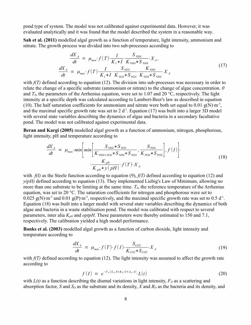
pond type of system. The model was not calibrated against experimental data. However, it was evaluated analytically and it was found that the model described the system in a reasonable way.

Sah et al. (2011) modelled algal growth as a function of temperature, light intensity, ammonium and nitrate. The growth process was divided into two sub-processes according to

dX A

dt= μmax⋅ f (T )⋅

IK I +I

⋅S NH4

K NH4+S NH4

⋅X A ,

dX A

dt= μmax⋅ f (T )⋅

IK I + I

⋅S NO3

K NO3+S NO3

⋅K NH4

K NH4+S NH4

⋅X A

(17)

with f(T) defined according to equation (12). The division into sub-processes was necessary in order to relate the change of a specific substrate (ammonium or nitrate) to the change of algae concentration. θ and T0, the parameters of the Arrhenius equation, were set to 1.07 and 20 °C, respectively. The light intensity at a specific depth was calculated according to Lambert-Beer's law as described in equation (10). The half saturation coefficients for ammonium and nitrate were both set equal to 0.01 g(N)·m-3, and the maximal specific growth rate was set to 2 d-1. Equation (17) was built into a larger 3D model with several state variables describing the dynamics of algae and bacteria in a secondary facultative pond. The model was not calibrated against experimental data.

Beran and Kargi (2005) modelled algal growth as a function of ammonium, nitrogen, phosphorous, light intensity, pH and temperature according to

dX A

dt= μmax⋅min[min [ S NH4 +S NO3

K NH4+NO3+S NH4+S NO3

,S PO4

K PO4+S PO4] , f ( I )]⋅

⋅K pH

K pH + y ( pH )⋅ f (T )⋅X A

(18)

with f(I) as the Steele function according to equation (9), f(T) defined according to equation (12) and y(pH) defined according to equation (13). They implemented Liebig's Law of Minimum, allowing no more than one substrate to be limiting at the same time. T0, the reference temperature of the Arrhenius equation, was set to 20 °C. The saturation coefficients for nitrogen and phosphorous were set to 0.025 g(N)·m-3 and 0.01 g(P)·m-3, respectively, and the maximal specific growth rate was set to 0.5 d-1. Equation (18) was built into a larger model with several state variables describing the dynamics of both algae and bacteria in a waste stabilisation pond. The model was calibrated with respect to several parameters, inter alia KpH and optpH. These parameters were thereby estimated to 150 and 7.1, respectively. The calibration yielded a high model performance.

Banks et al. (2003) modelled algal growth as a function of carbon dioxide, light intensity and temperature according to

dX A

dt= μmax⋅ f (T )⋅ f ( I )⋅

SCO2

KCO2+SCO2

⋅X A (19)

with f(T) defined according to equation (12). The light intensity was assumed to affect the growth rate according to

f (I ) = e−F D⋅(S D⋅S+B D⋅X +A D⋅A)⋅L(t) (20)

with L(t) as a function describing the diurnal variations in light intensity, FD as a scattering and absorption factor, S and SD as the substrate and its density, X and BD as the bacteria and its density, and

8

A and AD as the algae and its density. The half saturation coefficient for carbon dioxide was set to 0.044 g(CO2)·m-3, the maximal specific growth rate was set to 1.13 d-1 and the reference temperature of the Arrhenius equation T0 was set to 20 °C. Equation (19) was built into a larger model with several state variables describing the dynamics of both algae and bacteria in a facultative pond. The model was not calibrated. However, model output was compared to observed data indicating that the model predicted the system dynamics to some extent.

Dochain et al. (2003) modelled algal growth as a function of soluble substrate, hydrogen sulphide and light intensity according to

dX A

dt= μmax⋅(1−

k Q

Q)⋅X A ,

dQdt

= μmax⋅S S

K S+S S

⋅K H2S

K H2S +S H2S

⋅f (I )−μmax⋅(Q−k Q)(21)

with Q as the Droop parameter that represents the quantity of limiting elements and kQ as the minimal quantity of Q. The Droop function was used to describe a delay between limiting factors and their effect on growth.

Mashauri and Kayombo (2002) modelled algal growth as a function of carbon dioxide, light intensity, pH and temperature according to

dX A

dt= μmax⋅ f (T )⋅

IK I +I

⋅SCO2

KCO2+S CO2

⋅K pH

K pH+ y ( pH )⋅X A (22)

with f(T) as described by Jorgensen et al. (1978). The maximal specific growth rate was set to 2.55 d-1 while the half saturation coefficient for carbon dioxide was set to 0.5 g(CO2)·m-3. y(pH) was calculated according to equation (13) and the parameters KpH and optpH were estimated to 189 and 7.79, respectively. Equation (22) was built into a larger model with several state variables describing the dynamics of both algae and bacteria in a facultative pond. The model was validated against measurements from a real facultative pond indicating that the model managed to predict the system dynamics to some extent.

Moreno-Grau et al. (1996) proposed a model describing algal growth as a function of temperature, light intensity, ammonia and soluble phosphorous according to

dX A

dt= μmax⋅ f (T )⋅ f ( I )⋅

S NH3

K NH3+S NH3

⋅S P

K P+S P

⋅(1−X A

ηA)⋅X A (23)

with f(T) defined according to equation (12) and f(I) defined as the Steele function. The parameter ηA defines an upper limit for the algae concentration. θ and T0, the parameters of the Arrhenius equation, were set to 1.07 and 20 °C, respectively, and the maximal specific growth rate was set to 0.5 d-1. Equation (23) was built into a larger model with several state variables describing the dynamics of, inter alia, algae, bacteria and zoo-plankton in a wastewater pond. Model output was compared to measurements indicating a good model performance.

Carberry and Greene (1992) proposed a model describing algal growth as a function of light intensity and carbon dioxide according to

dX A

dt= μmax⋅min( f ( I ) ,

S CO2

K CO2+SCO2)⋅X A (24)

9

with f(I) equal to zero during night and equal to a positive number smaller than one during daytime. They implemented Liebig's Law of Minimum, allowing no more than one factor to limit growth at the same time. The maximal specific growth rate was set to 0.98 d-1 and the half saturation coefficient for carbon dioxide was set to 0.03 g(CO2)·m-3. Equation (24) was built into a larger model with several state variables describing the dynamics of algae and bacteria in an algae-bacteria-clay treatment system. The model was not calibrated or evaluated against experimental data. However, it was evaluated analytically and it was shown that the model managed to describe the system dynamics in a reasonable way.

Buhr and Miller (1983) proposed a model describing algal growth as a function of light intensity, carbon dioxide and total inorganic nitrogen according to

dX A

dt= μmax⋅ f ( I )⋅

S CO2

KCO2+SCO2

⋅S NH4 +S NO3

K NH4+NO3+S NH4+S NO3

⋅X A (25)

with f(I) defined as a square wave function equal to zero during the night and equal to one during daytime. The maximal specific growth rate was set to 0.9991 d-1 and the half saturation coefficients for carbon dioxide and total inorganic nitrogen were both set to 0.001 mol·m-3. Equation (25) was built into a larger model with several state variables describing the dynamics of algae and bacteria in a high-rate algae-bacteria treatment pond. The model was validated against experimental data and was shown to describe the real system well.

2.2.3 Processes reducing the concentration of algae

Several processes counteract algal growth by affecting the algae concentration negatively. The processes of death and respiration are present irrespective of system set-up while the existence of other processes, such as predation, grazing and sedimentation, depends upon the system set-up. Some models include only one process reducing the concentration of algae. The process is then defined as algal decay according to

dX A

dt= −b⋅X A (26)

with b as the decay coefficient (Buhr and Miller, 1983; Decostere et al., 2013; Yang, 2011). This process has also been described as a function of temperature (Sah et al., 2011) by multiplying equation (26) with the Arrhenius equation, and as a function of dissolved oxygen (Dochain et al., 2003) according to

dX A

dt= −b⋅(1−

S O2

KO2+SO2)⋅X A . (27)

Since those models only include one process reducing the concentration of algae, the process must necessarily represent both death and respiration.

Beran and Kargi (2005) proposed a model including basal metabolism, sedimentation and grazing. Respiration is part of the basal metabolism and algal death was included in the sedimentation process since they assumed the sedimentation to be a direct result of algal death. They assumed the concentration of zoo-plankton to be a constant fraction of the concentration of algae, making the process of gazing proportional to the algae concentration. Other models that include several processes reducing the concentration of algae have been proposed by Mesplé et al. (1996) (including death and

10

grazing), Moreno-Grau et al. (1996) (including death, respiration and sedimentation), and Colomer and Rico (1993) (including decomposition and sedimentation).

2.2.4 Summary of kinetic parameters

The kinetic parameters presented earlier in this section were rewritten and expressed in the same units in order to allow straightforward comparisons (Table 1).

Table 1. Kinetic parameters used in the models presented in this section

Parameter Value Description Unit

μmax 0.79 a, 0.48-0.52 b, 0.9991 c, j, 2 d, 0.5 e, h, 1.13 f, 2.55 g, 0.98 i

Maximal specific growth rate [d-1]

KN 9.5 ± 2.9 a Saturation coefficient for total nitrogen [g(N)·m-3]

KNH4+NO3 0.025 e, 0.014 c, j Saturation coefficient for ammonium plus nitrate [g(N)·m-3]

KNH4 0.01 d Saturation coefficient for ammonium [g(N)·m-3]

KNO3 0.01 d Saturation coefficient for nitrite [g(N)·m-3]

KPO4 0.01 e Saturation coefficient for phosphorous [g(P)·m-3]

KCO2 0.055 b, 0.012 c, f, j, 0.14 g, 0.0082 i

Saturation coefficient for carbon dioxide [g(C)·m-3]

KpH 150 e, 189 g Saturation coefficient for pH [-]

optpH 7.1 e, 7.79 g Optimal pH value [-]

θ 1.07 d, h Temperature coefficient of the Arrhenius equation [-]

T0 20 d, e, f, h Reference temperature in the Arrhenius equation [°C]

b 0.01 b, 0.05 c, j, 0.1 d Decay rate [d-1]a (Wu et al., 2013). b (Decostere et al., 2013). c (Yang, 2011). d (Sah et al., 2011). e (Beran and Kargi, 2005). f (Banks et al., 2003). g (Mashauri and Kayombo, 2002). h (Moreno-Grau et al., 1996). i (Carberry and Greene, 1992). j (Buhr and Miller, 1983).

2.3 GAS EXCHANGE

The oxygen and carbon dioxide concentrations in an activated sludge basin are govern by the water-atmosphere gas exchange. It makes the concentrations converge towards their respective saturation values according to equation (30) and (31). The saturation value of gas G may be calculated using Henry's law according to

G SAT = k H ,G⋅PG (28)

with GSAT as the saturation value, kH,G as Henry's constant and PG as the partial pressure (Atkins and Jones, 2008).

11

The concentrations can also be governed through active management in terms of aeration or carbon dioxide injection, and these processes can also be described by equation (30) and (31). The combined effect of the water-atmosphere gas exchange and the gas injection can be modelled in different ways. Yang (2011) separated the processes and modelled the combined effect according to

d (S G)

dt= wG+ f G (29)

with SG as the gas concentration in the water column, wG representing the water-atmosphere gas exchange and fG representing the gas injection. The separation into different terms allows a detailed process description. A less complex alternative to this approach is to describe the two processes with one term rather than two. This was done within BSM1 presented in section 3.2.

The gas exchange of oxygen, referred to as the oxygen transfer rate (O2TR), can be described according to

O2TR = K L aO2⋅(O2SAT−S O2) (30)

where KLaO2 defines how fast oxygen is transferred to or from the water column, O2SAT is the oxygen saturation value and SO2 is the dissolved oxygen concentration in the water column. Equation (30) has been implemented in models proposed by Decostere et al. (2013), Dochain et al. (2003) and Mashauri and Kayombo (2002). It has also been implemented in BSM1 presented in section 3.2, and in an AQUASIM application of RWQM1 presented in section 3.3. RWQM1 was implemented in AQUASIM by Peter Reichert and the AQUASIM file needed to run the program is provided at his homepage (Reichert, 2014). The parameter values governing the gas exchange of oxygen used in these models are summarized in Table 2.

Within BSM1, more thoroughly presented in section 3.2, the KLaO2 value was allowed to vary between 0 d-1 representing a non-aerated basin, and 360 d-1 representing strong aeration, and the oxygen saturation value was set to 8 g(O)·m-3 (Alex et al., 2008b). BSM1 was developed to describe an activated sludge process.

In the AQUASIM application the KLaO2 value and the dissolved oxygen saturation value were both temperature dependent. For a temperature of 20 °C, they equalled 20 d-1 and 9.0953 g(O)·m-3, respectively. No aeration was assumed and the equation was used to describe oxygen transports both to and from the water column. RWQM1 represents a river system why its KLaO2 value is likely to be larger than for an activated sludge basin without aeration. The relatively large surface area and the turbulence of the river facilitates gas transports between water and atmosphere.

Decostere et al. (2013) estimated the KLaO2 value of a reactor empirically and found that the value varied between 15.84 d-1 and 26.79 d-1. They calculated the oxygen saturation value as a function of temperature. For a temperature of 20 °C, it equalled 9.0236 g(O)·m-3. They used equation (30) in order to describe the dissolved oxygen concentration of a 1 L reactor containing an algae population of Chlorella vulgaris. The oxygen concentration of the reactor varied around the saturation value and the model gave a good prediction of observed values. Hence, their model managed to describe oxygen transfer both to and from the water column. The reactor was mixed through air sparging why the estimated KLaO2 values are likely to be larger than for an activated sludge basin without aeration.

Dochain et al. (2003) estimated the KLaO2 value empirically to 0.24 d-1. They included equation (30) in a model describing algae and bacteria dynamics and calibrated the model against measured dissolved oxygen data. In the same way they estimated the oxygen saturation value to 10 g(O)·m-3. The relatively

12

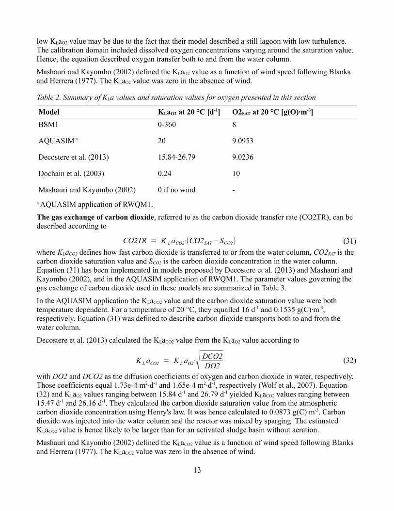
low KLaO2 value may be due to the fact that their model described a still lagoon with low turbulence. The calibration domain included dissolved oxygen concentrations varying around the saturation value. Hence, the equation described oxygen transfer both to and from the water column.

Mashauri and Kayombo (2002) defined the KLaO2 value as a function of wind speed following Blanks and Herrera (1977). The KLaO2 value was zero in the absence of wind.

Table 2. Summary of KLa values and saturation values for oxygen presented in this section

Model KLaO2 at 20 °C [d-1] O2SAT at 20 °C [g(O)·m-3]

BSM1 0-360 8

AQUASIM a 20 9.0953

Decostere et al. (2013) 15.84-26.79 9.0236

Dochain et al. (2003) 0.24 10

Mashauri and Kayombo (2002) 0 if no wind -

a AQUASIM application of RWQM1.

The gas exchange of carbon dioxide, referred to as the carbon dioxide transfer rate (CO2TR), can be described according to

CO2TR = K L aCO2⋅(CO2SAT−SCO2) (31)

where KLaCO2 defines how fast carbon dioxide is transferred to or from the water column, CO2SAT is the carbon dioxide saturation value and SCO2 is the carbon dioxide concentration in the water column. Equation (31) has been implemented in models proposed by Decostere et al. (2013) and Mashauri and Kayombo (2002), and in the AQUASIM application of RWQM1. The parameter values governing the gas exchange of carbon dioxide used in these models are summarized in Table 3.

In the AQUASIM application the KLaCO2 value and the carbon dioxide saturation value were both temperature dependent. For a temperature of 20 °C, they equalled 16 d-1 and 0.1535 g(C)·m-3, respectively. Equation (31) was defined to describe carbon dioxide transports both to and from the water column.

Decostere et al. (2013) calculated the KLaCO2 value from the KLaO2 value according to

K L aCO2 = K L aO2⋅√ DCO2DO2

(32)

with DO2 and DCO2 as the diffusion coefficients of oxygen and carbon dioxide in water, respectively. Those coefficients equal 1.73e-4 m2·d-1 and 1.65e-4 m2·d-1, respectively (Wolf et al., 2007). Equation (32) and KLaO2 values ranging between 15.84 d-1 and 26.79 d-1 yielded KLaCO2 values ranging between 15.47 d-1 and 26.16 d-1. They calculated the carbon dioxide saturation value from the atmospheric carbon dioxide concentration using Henry's law. It was hence calculated to 0.0873 g(C)·m-3. Carbon dioxide was injected into the water column and the reactor was mixed by sparging. The estimated KLaCO2 value is hence likely to be larger than for an activated sludge basin without aeration.

Mashauri and Kayombo (2002) defined the KLaCO2 value as a function of wind speed following Blanks and Herrera (1977). The KLaCO2 value was zero in the absence of wind.

13

Table 3. Summary of KLa values and saturation values for carbon dioxide presented in this section

Model KLaCO2 at 20 °C [d-1] CO2SAT at 20 °C [g(C)·m-3]

AQUASIM a 16 0.1535

Decostere et al. (2013) 16.2-27.43 0.0873

Mashauri and Kayombo (2002) 0 if no wind -

a AQUASIM application of RWQM1.

14

3 SIMULATION MODELS

Three models were used in this study: ASM1, BSM1 and RWQM1. RWQM1 was used as the starting point for model development while ASM1 and BSM1 were used in model evaluation and calibration.

3.1 THE ACTIVATED SLUDGE MODEL NO. 1

The Activated Sludge Model No. 1, abbreviated ASM1, is a widely spread and acknowledged model describing the dynamics of heterotrophic and autotrophic bacteria in a wastewater treatment environment. Henze et al. (1987) provide a comprehensive model description and a Gujer matrix summarizing the model. The Gujer matrix is presented in Appendix A.

Table 4. State variables included in ASM1

State variable Description Unit

SI Soluble inert organic matter [g(COD)·m-3]

SS Readily biodegradable substrate [g(COD)·m-3]

XI Particulate inert organic matter [g(COD)·m-3]

XS Slowly biodegradable substrate [g(COD)·m-3]

XB,H Active heterotrophic biomass [g(COD)·m-3]

XB,A Active autotrophic biomass [g(COD)·m-3]

XP Particulate products arising from biomass decay [g(COD)·m-3]

SO Oxygen [g(O)·m-3]

SNO Nitrate and nitrite nitrogen [g(N)·m-3]

SNH Ammonium and ammonia nitrogen [g(N)·m-3]

SND Soluble biodegradable organic nitrogen [g(N)·m-3]

XND Particulate biodegradable organic nitrogen [g(N)·m-3]

SALK Alkalinity [mol·m-3]

ASM1 consists of 13 differential equations defining the dynamics of 13 state variables (Table 4). All state variables except soluble and particulate inert organic matter are affected by one or several out of eight processes. The relationship between a state variable and the processes that affect it is defined by stoichiometric coefficients according to

dS j

dt= ∑

i=1

8

e i , j⋅pi (33)

with Sj as state variable j, ei,j as the stoichiometric coefficient relating process i to state variable j, and pi

as process i.

The processes describe bacterial growth, bacterial decay, ammonification and hydrolysis. Monod functions describe how the growth processes are affected by limiting substrates and switching functions

15

makes aerobic growth prevalent under aerobic conditions and anoxic growth prevalent under anoxic conditions. The processes of decay were assumed to incorporate several processes such as metabolism, death, predation and lysis (Henze et al., 1987). However, they were described with relatively simple equations, first order with respect to the heterotrophic or the autotrophic biomass. Hydrolysis is the process in which slowly biodegradable substrate is turned into readily biodegradable substrate. The hydrolysis process included in ASM1 is defined according to

k h⋅X S/ X B , H

K X + X S / X B , H

⋅( SO2

K O2+S O2

+ηh⋅K O2

KO2+SO2

⋅S NO

K NO+S NO)⋅X B , H . (34)

It is assumed that the hydrolysis rate is first order with respect to heterotrophic biomass, and that the rate saturates as the concentration of slowly biodegradable substrate largely exceeds the concentration of heterotrophic bacteria. It is also assumed that the process is dependent on enzymes and that the enzyme production is dependent on the availability of electron acceptors. This is represented by the Monod functions for oxygen and nitrate plus nitrite.

Nitrification is known to be affected by pH (Henze et al., 1987). This dependency was not included in ASM1 due to the difficulties in estimating pH dynamics. Therefore, ASM1 may only be used to simulate systems with neutral pH. The alkalinity is estimated as a control tool. An alkalinity below 1 mol·m-3 indicates an unstable pH that may drop to values well below 6 (Henze et al., 1987). An other assumption affecting the application domain of ASM1 is the absence of phosphorous limitation. ASM1 may only be used to describe systems were phosphorous is non-limiting.

3.2 THE BENCHMARK SIMULATION MODEL NO. 1

The Benchmark Simulation Model no. 1, abbreviated BSM1, is a widely spread and acknowledged framework that is used to simulate an activated sludge process in order to evaluate control and operation strategies. It was completed by the IWA Task Group on Benchmarking of Control Strategies and they provide a comprehensive model description (Alex et al., 2008b). The model software is free and can be downloaded from the Department of Industrial Electrical Engineering and Automation at Lund University (Alex et al., 2008a).

BSM1 is based on an activated sludge process structure that can be implemented in Simulink. The structure represents a conventional treatment process with internal recirculation, a five-compartment water basin and a settler (Figure 2). All compartments are subject to biochemical processes that are described by the differential equations of ASM1, defined in a C-function. The settler is described as a ten layered unit. Aeration may be implemented in all compartments but are by default only implemented in the last three, representing a pre-denitrification process. Several sets of dynamic influent driving data are available representing different weather conditions, as is a set of constant influent driving data (Table 5). The wastewater treatment process may be simulated as open loop without active controllers, or as closed loop, for control strategy analysis.

16

Table 5. Influent data provided within the BSM1 framework

State variable Influent value Unit

SI 30 [g(COD)·m-3]

SS 69.5 [g(COD)·m-3]

XI 51.2 [g(COD)·m-3]

XS 202.32 [g(COD)·m-3]

XB,H 28.17 [g(COD)·m-3]

XB,A 0 [g(COD)·m-3]

XP 0 [g(COD)·m-3]

SO2 0 [g(O)·m-3]

SNO 0 [g(N)·m-3]

SNH 31.56 [g(N)·m-3]

SND 6.95 [g(N)·m-3]

XND 10.59 [g(N)·m-3]

SALK 7 [mol·m-3]

Q 18 446 [m³·d-1]

3.3 THE RIVER WATER QUALITY MODEL NO. 1

The River Water Quality Model no. 1, abbreviated RWQM1, is a model describing the dynamics of heterotrophic and autotrophic bacteria, zoo-plankton and algae in a river water environment. Reichert et al. (2001) provide a comprehensive model description and a Gujer matrix summarizing the model. The Gujer matrix is presented in Appendix B.

Just like ASM1, RWQM1 consists of a set of differential equations governing the change of model state variables (Table 6). Despite the similarities in model structure and representation there are several major differences between RWQM1 and ASM1, of which three are of special interest. Firstly, the model application domains differ. RWQM1 was developed to describe a river water system while

17

Figure 2. Basic description of the BSM1 structure. Aeration is applied to the three last compartments representing pre-denitrification.

Influent

Effluent

WasteSludge recirculationInternal

recirculation

SedimentationWater basin

ASM1 was developed to describe a wastewater treatment system. Secondly, RWQM1 is much larger in terms of the number of included state variables and processes. The large model size is a consequence of the relatively complex application domain that includes algae and pH dynamics. Algae constitute an important element in a typical river system and algae dynamics have a relatively large impact on the pH value. In order to describe such a system accurately it is necessary to model pH variations. This requires the inclusion of several chemical equilibria that affect the pH value, and the corresponding state variables. Thirdly, the organic state variables of RWQM1 are described not only in terms of COD units but also in terms of dry weight. Each organic state variable is assumed to consist of the elements carbon, hydrogen, oxygen, nitrogen and phosphorous, and elemental mass fractions are explicitly defined for each one of them. Reichert et al. (2001) provide a formula based on these mass fractions connecting COD units to dry weight.

Stoichiometric coefficients were calculated from the elemental composition of organic state variables, stoichiometric parameters and the principle of mass conservation, a method presented by Reichert and Schuwirth (2010). This method ensures that the total mass of a certain element remains constant within a closed system. It can be used to strengthen or impugn empirically determined stoichiometric coefficients. A limitation of the RWQM1 is that it may be unable to describe systems in which other elements than those explicitly defined as mass fractions are abundant. A water with a lot of siliceous diatoms is an example of such a system.

Due to the large model size and the complex formulae used to calculate the stoichiometric coefficients the Gujer matrix lacks process equations and stoichiometric coefficients. The stoichiometric coefficients are presented in Appendix C and they may be downloaded from Peter Reichert's homepage (Reichert, 2014). The process equations are presented in Appendix D. Some of the processes were of special interest in this study and they are presented below.

Aerobic growth of heterotrophic bacteria on ammonium:

k gro , H , aer⋅eβH⋅(T −T 0)⋅S S

K S +S S

⋅S O2

KO2+SO2

⋅S NH4+S NH3

K N , H ,aer +S NH4+S NH3

⋅

⋅S HPO4+S H2PO4

K PO4+S HPO4+S H2PO4

⋅X H

(35)

Aerobic growth of heterotrophic bacteria on nitrate:

k gro , H , aer⋅eβH⋅(T −T 0)⋅S S

K S +S S

⋅S O2

KO2+SO2

⋅K N , H , aer

K N , H ,aer +S NH4+S NH3

⋅

⋅S NO3

K N , H ,aer +S NO3

⋅S HPO4+S H2PO4

K PO4+S HPO4+S H2PO4

⋅X H

(36)

Anoxic growth of heterotrophic bacteria on nitrate:

k gro , H , anox⋅eβH⋅(T −T0 )⋅S S

K S+S S

⋅KO2

K O2+S O2

⋅S NO3

K NO3 , H ,anox+S NO3

⋅S HPO4+S H2PO4

K PO4+S HPO4+S H2PO4

⋅X H (37)

Anoxic growth of heterotrophic bacteria on nitrite:

k gro , H , anox⋅eβH⋅(T −T0 )⋅S S

K S+S S

⋅KO2

K O2+S O2

⋅S NO2

K NO2 , H ,anox+S NO2

⋅S HPO4+S H2PO4

K PO4+S HPO4+S H2PO4

⋅X H (38)

18

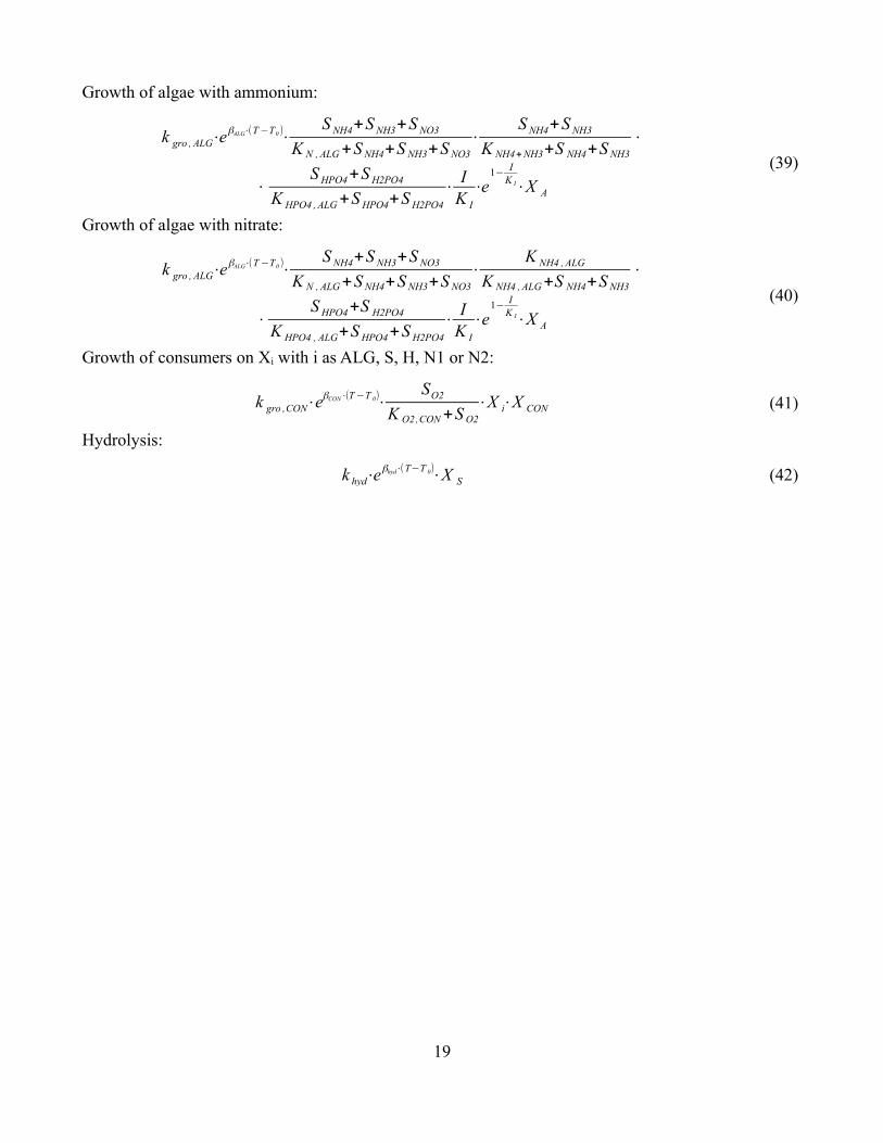
Growth of algae with ammonium:

k gro , ALG⋅eβALG⋅(T −T0 )⋅S NH4+S NH3+S NO3

K N , ALG+S NH4+S NH3+S NO3

⋅S NH4+S NH3

K NH4+NH3+S NH4+S NH3

⋅

⋅S HPO4+S H2PO4

K HPO4 , ALG+S HPO4+S H2PO4

⋅I

K I

⋅e1− I

K I⋅X A

(39)

Growth of algae with nitrate:

k gro , ALG⋅eβALG⋅(T −T0 )⋅S NH4+S NH3+S NO3

K N , ALG+S NH4+S NH3+S NO3

⋅K NH4 , ALG

K NH4 , ALG+S NH4+S NH3

⋅

⋅S HPO4+S H2PO4

K HPO4 , ALG+S HPO4+S H2PO4

⋅I

K I

⋅e1−

IK I⋅X A

(40)

Growth of consumers on Xi with i as ALG, S, H, N1 or N2:

k gro ,CON⋅eβCON⋅(T −T 0)⋅SO2

K O2 ,CON +S O2

⋅X i⋅X CON (41)

Hydrolysis:

k hyd⋅eβhyd⋅(T−T 0)⋅X S (42)

19

Table 6. State variables included in RWQM1

State variable

Corresponding ASM1 variable

Description Unit

SS SS, SND a Readily biodegradable substrate [g(COD)·m-3]

SI SI Soluble inert organic matter [g(COD)·m-3]

SNH4 SNH Ammonium [g(N)·m-3]

SNH3 SNH Ammonia [g(N)·m-3]

SNO2 SNO Nitrite [g(N)·m-3]

SNO3 SNO Nitrate [g(N)·m-3]

SHPO4 - Hydrogen phosphate [g(P)·m-3]

SH2PO4 - Dihydrogen phosphate [g(P)·m-3]

SO2 SO2 Dissolved oxygen [g(O)·m-3]

SCO2 - Carbon dioxide [g(C)·m-3]

SHCO3 - Bicarbonate [g(C)·m-3]

SCO3 - Carbon trioxide [g(C)·m-3]

SH SALK Hydrogen [mol·m-3]

SOH - Hydroxide [mol·m-3]

SCa - Calcium [g(Ca)·m-3]

XH XB,H Active heterotrophic biomass [g(COD)·m-3]

XN1 XB,A First stage nitrifiers [g(COD)·m-3]

XN2 XB,A Second stage nitrifiers [g(COD)·m-3]

XALG - Algae [g(COD)·m-3]

XCON - Consumers (zoo-plankton) [g(COD)·m-3]

XS XS, XND a Slowly biodegradable substrate [g(COD)·m-3]

XI XI+XP Particulate inert organic matter [g(COD)·m-3]a The RWQM1 state variables of readily and slowly biodegradable substrate are associated with nitrogen mass fractions. Hence, they correspond to the ASM1 state variables of SS and SND, and XS and XND, respectively.

20

4 SIMULINK IMPLEMENTATION OF THE ACTIVATED SLUDGE MODEL NO. 1

A model set-up based on ASM1 was implemented in Simulink. The model set-up was to be used as a tool for evaluation and calibration in the development of an algae based activated sludge model based on RWQM1.

The differential equations of ASM1 were implemented in a Matlab S-function that was evaluated through comparisons with the ASM1 C-function used within the BSM1 framework. Consistency between the two functions was considered to indicate a correct code implementation.

An activated sludge process consisting of one completely mixed basin and ideal sedimentation was modelled in Simulink. The system dynamics of the basin were described by the ASM1 differential equations as implemented in the S-function. A quality control of the model set-up was conducted through comparisons with BSM1.

4.1 IMPLEMENTATION AND EVALUATION OF THE DIFFERENTIAL EQUATIONS THAT DEFINE THE ACTIVATED SLUDGE MODEL NO. 1

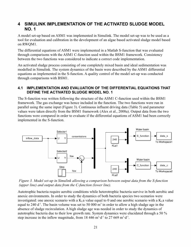
The S-function was written following the structure of the ASM1 C-function used within the BSM1 framework. The gas exchange was hence included in the function. The two functions were run in parallel using the same input (Figure 3). Continuous influent driving data (Table 5) and parameter values were taken directly from the BSM1 framework (Alex et al., 2008a). Output data from the two functions were compared in order to evaluate if the differential equations of ASM1 had been correctly implemented in the S-function.

Autotrophic bacteria require aerobic conditions while heterotrophic bacteria survive in both aerobic and anoxic environments. In order to study the dynamics of both bacteria species two scenarios were investigated: one anoxic scenario with a KLa value equal to 0 and one aerobic scenario with a KLa value equal to 240 d-1. The basin volume was set to 50 000 m3 in order to allow a high sludge age in the absence of sludge recirculation. A high sludge age was needed in order to study the dynamics of autotrophic bacteria due to their low growth rate. System dynamics were elucidated through a 50 % step increase in the inflow magnitude, from 18 446 m3·d-1 to 27 669 m3·d-1.

21

Figure 3. Model set-up in Simulink allowing a comparison between output data from the S-function (upper line) and output data from the C-function (lower line).

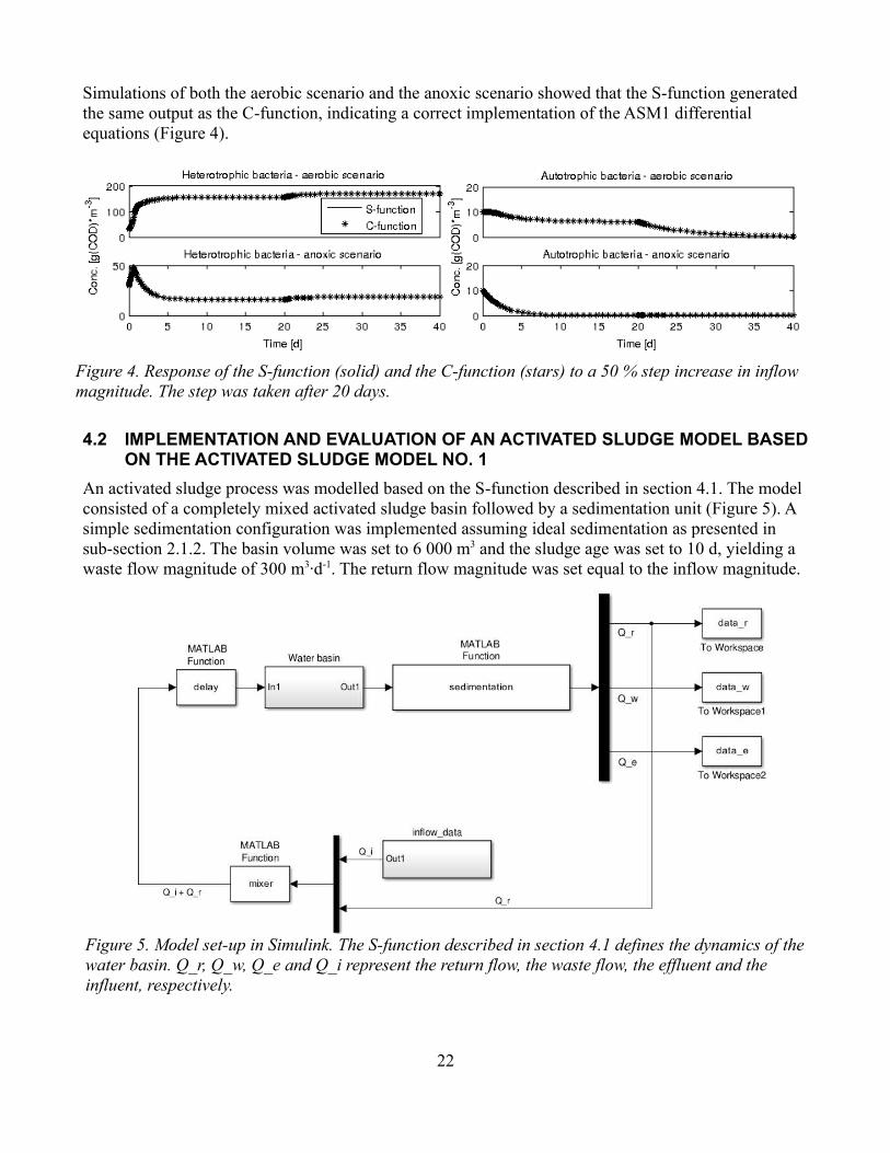
Simulations of both the aerobic scenario and the anoxic scenario showed that the S-function generated the same output as the C-function, indicating a correct implementation of the ASM1 differential equations (Figure 4).

4.2 IMPLEMENTATION AND EVALUATION OF AN ACTIVATED SLUDGE MODEL BASED ON THE ACTIVATED SLUDGE MODEL NO. 1

An activated sludge process was modelled based on the S-function described in section 4.1. The model consisted of a completely mixed activated sludge basin followed by a sedimentation unit (Figure 5). A simple sedimentation configuration was implemented assuming ideal sedimentation as presented in sub-section 2.1.2. The basin volume was set to 6 000 m3 and the sludge age was set to 10 d, yielding a waste flow magnitude of 300 m3·d-1. The return flow magnitude was set equal to the inflow magnitude.

22

Figure 4. Response of the S-function (solid) and the C-function (stars) to a 50 % step increase in inflow magnitude. The step was taken after 20 days.

Figure 5. Model set-up in Simulink. The S-function described in section 4.1 defines the dynamics of the water basin. Q_r, Q_w, Q_e and Q_i represent the return flow, the waste flow, the effluent and the influent, respectively.

The ASM1 set-up described above was quality controlled through comparisons with the open loop version of BSM1. The comparison was focused on steady state values under both aerobic (KLa = 240 d-1) and anoxic (KLa = 0 d-1) conditions. For consistency between the models the internal recirculation of BSM1 was set to zero and the magnitude of the waste flow was set to 300 m3·d-1. Both models were driven by constant influent data taken from the BSM1 framework (Table 5). Simulations were conducted with an ode15s solver and a relative tolerance of 1e-13. The basin volume of BSM1 is divided into five compartments of which the last one was used in the comparison.

The comparison revealed that the two models were relatively consistent in terms of the steady state values of all investigated state variables (Table 7), indicating that the ASM1 set-up was adequate for describing an activated sludge process. Both models reflected the fact that an anoxic environment aggravates the growth of heterotrophic bacteria and prohibits the growth of autotrophic bacteria, and that the extinction of nitrifiers prohibits the nitrification process resulting in low nitrate and nitrite concentrations and high ammonium and ammonia concentrations. The settler included in the ASM1 set-up was based on ideal sedimentation while the settler in BSM1 was described as a 10 layered unit accounting for settling velocity. Small inconsistencies in steady state values were hence expected.

Table 7. Steady state values of some state variables in the activated sludge basin under aerobic and anoxic conditions according to the ASM1 set-up and BSM1

State variable Aerobic scenario Anoxic scenario Unit

ASM1 set-up BSM1a ASM1 set-up BSM1a

Heterotrophic bacteria 3029 2887 217 202 [g(COD)·m-3]

Autotrophic bacteria 200 188 0 0 [g(COD)·m-3]

Dissolved oxygen 4 6 0 0 [g(O)·m-3]

Alkalinity 2.1 2.3 7.4 7.4 [mol·m-3]

Nitrate plus nitrite 38 34 0 0 [g(N)·m-3]

Ammonium plus ammonia 0.5 0.1 37 38 [g(N)·m-3]

Readily biodegradable substrate 1.0 0.6 69.5 69.5 [g(COD)·m-3]

Slowly biodegradable substrate 59 37 6918 5512 [g(COD)·m-3]a Steady state values taken from the last compartment.

23

5 SIMULINK IMPLEMENTATION OF THE RIVER WATER QUALITY MODEL NO. 1

The differential equations of RWQM1 were implemented in a Matlab S-function following the structure of the S-function presented in section 4.1. An activated sludge process was modelled in Simulink based on the RWQM1 S-function following the structure of the ASM1 set-up described in section 4.2. A comparison was then made between the system dynamics of the RWQM1 set-up and the system dynamics of the ASM1 set-up. This was done to evaluate how well the RWQM1 set-up described an activated sludge process. The algae dynamics of RWQM1 were excluded in order to allow a straightforward comparison between the two models. It should be emphasized that the comparison was motivated by the fact that RWQM1 was developed to describe a river system and not an activated sludge basin.

5.1 IMPLEMENTATION OF THE DIFFERENTIAL EQUATIONS THAT DEFINE THE RIVER WATER QUALITY MODEL NO. 1

The differential equations of RWQM1 were written in a S-function that is presented in Appendix E. It had the same structure as the S-function used in the ASM1 set-up presented in section 4.1, and hence the same structure as the ASM1 C-function used within the BSM1 set-up. The equations were simplified in that the light intensity dependency of algal growth, described in equation (39) and equation (40), was neglected. It was assumed that the light intensity at the light source can be kept constant and that the change of light attenuation due to variations in biomass concentration may be neglected. Some other modifications, coupled to the representation of gas exchange, were done in order to make the model fit into an activated sludge environment. Those are presented in this section.

Gas exchange processes, as described in section 2.3, are essential for a correct description of dissolved oxygen and carbon dioxide dynamics of an activated sludge environment. No such processes were included in the differential equations that define RWQM1. The differential equations governing the change of dissolved oxygen and carbon dioxide were hence adjusted to account for gas exchange. The possibility of aeration and carbon dioxide injection was built into the RWQM1 set-up allowing the user to choose one out of four different gas exchange scenarios.

The first scenario represented an activated sludge basin with neither aeration nor carbon dioxide injection (Table 9). Oxygen and carbon dioxide exchange between the water column and the atmosphere were described by equation (30) and (31), respectively. Saturation values were calculated according to Henry's law (Table 8).

Table 8. Values used in Henry's law and the corresponding calculated saturation values

Gas (G) kH,G [mol·L-1·atm-1] PG [atm] GSAT [mol·L-1] GSAT

Oxygen 1.3e-3 a 0.21 a 2.73e-4 8.736 g(O)·m-3

Carbon dioxide 2.3e-2 a 392.52e-6 9.03e-6 0.11 g(C)·m-3

aAtkins and Jones (2008).

The partial carbon dioxide pressure was calculated according to

PCO2 = xCO2⋅P (43)

24

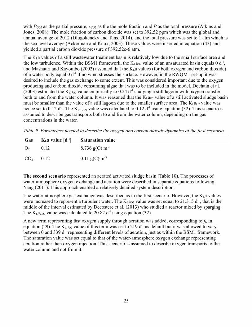
with PCO2 as the partial pressure, xCO2 as the the mole fraction and P as the total pressure (Atkins and Jones, 2008). The mole fraction of carbon dioxide was set to 392.52 ppm which was the global and annual average of 2012 (Dlugokencky and Tans, 2014), and the total pressure was set to 1 atm which is the sea level average (Ackerman and Knox, 2003). These values were inserted in equation (43) and yielded a partial carbon dioxide pressure of 392.52e-6 atm.

The KLa values of a still wastewater treatment basin is relatively low due to the small surface area and the low turbulence. Within the BSM1 framework, the KLaO2 value of an unsaturated basin equals 0 d-1, and Mashauri and Kayombo (2002) assumed that the KLa values (for both oxygen and carbon dioxide) of a water body equal 0 d-1 if no wind stresses the surface. However, in the RWQM1 set-up it was desired to include the gas exchange to some extent. This was considered important due to the oxygen producing and carbon dioxide consuming algae that was to be included in the model. Dochain et al. (2003) estimated the KLaO2 value empirically to 0.24 d-1 studying a still lagoon with oxygen transfer both to and from the water column. It was reasoned that the KLaO2 value of a still activated sludge basin must be smaller than the value of a still lagoon due to the smaller surface area. The KLaO2 value was hence set to 0.12 d-1. The KLaCO2 value was calculated to 0.12 d-1 using equation (32). This scenario is assumed to describe gas transports both to and from the water column, depending on the gas concentrations in the water.

Table 9. Parameters needed to describe the oxygen and carbon dioxide dynamics of the first scenario

Gas KLa value [d-1] Saturation value

O2 0.12 8.736 g(O)·m-3

CO2 0.12 0.11 g(C)·m-3

The second scenario represented an aerated activated sludge basin (Table 10). The processes of water-atmosphere oxygen exchange and aeration were described in separate equations following Yang (2011). This approach enabled a relatively detailed system description.

The water-atmosphere gas exchange was described as in the first scenario. However, the KLa values were increased to represent a turbulent water. The KLaO2 value was set equal to 21.315 d-1, that is the middle of the interval estimated by Decostere et al. (2013) who studied a reactor mixed by sparging. The KLaCO2 value was calculated to 20.82 d-1 using equation (32).

A new term representing fast oxygen supply through aeration was added, corresponding to fG in equation (29). The KLaO2 value of this term was set to 219 d-1 as default but it was allowed to vary between 0 and 339 d-1 representing different levels of aeration, just as within the BSM1 framework. The saturation value was set equal to that of the water-atmosphere oxygen exchange representing aeration rather than oxygen injection. This scenario is assumed to describe oxygen transports to the water column and not from it.

25

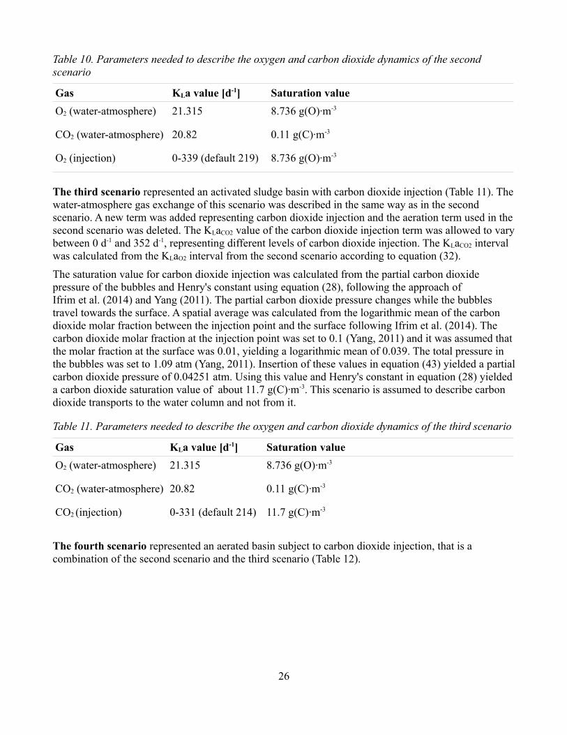
Table 10. Parameters needed to describe the oxygen and carbon dioxide dynamics of the second scenario

Gas KLa value [d-1] Saturation value

O2 (water-atmosphere) 21.315 8.736 g(O)·m-3

CO2 (water-atmosphere) 20.82 0.11 g(C)·m-3

O2 (injection) 0-339 (default 219) 8.736 g(O)·m-3

The third scenario represented an activated sludge basin with carbon dioxide injection (Table 11). The water-atmosphere gas exchange of this scenario was described in the same way as in the second scenario. A new term was added representing carbon dioxide injection and the aeration term used in the second scenario was deleted. The KLaCO2 value of the carbon dioxide injection term was allowed to vary between 0 d-1 and 352 d-1, representing different levels of carbon dioxide injection. The KLaCO2 interval was calculated from the KLaO2 interval from the second scenario according to equation (32).

The saturation value for carbon dioxide injection was calculated from the partial carbon dioxide pressure of the bubbles and Henry's constant using equation (28), following the approach of Ifrim et al. (2014) and Yang (2011). The partial carbon dioxide pressure changes while the bubbles travel towards the surface. A spatial average was calculated from the logarithmic mean of the carbon dioxide molar fraction between the injection point and the surface following Ifrim et al. (2014). The carbon dioxide molar fraction at the injection point was set to 0.1 (Yang, 2011) and it was assumed that the molar fraction at the surface was 0.01, yielding a logarithmic mean of 0.039. The total pressure in the bubbles was set to 1.09 atm (Yang, 2011). Insertion of these values in equation (43) yielded a partial carbon dioxide pressure of 0.04251 atm. Using this value and Henry's constant in equation (28) yielded a carbon dioxide saturation value of about 11.7 g(C)·m-3. This scenario is assumed to describe carbon dioxide transports to the water column and not from it.

Table 11. Parameters needed to describe the oxygen and carbon dioxide dynamics of the third scenario

Gas KLa value [d-1] Saturation value

O2 (water-atmosphere) 21.315 8.736 g(O)·m-3

CO2 (water-atmosphere) 20.82 0.11 g(C)·m-3

CO2 (injection) 0-331 (default 214) 11.7 g(C)·m-3

The fourth scenario represented an aerated basin subject to carbon dioxide injection, that is a combination of the second scenario and the third scenario (Table 12).

26

Table 12. Parameters needed to describe the oxygen and carbon dioxide dynamics of the fourth scenario

Gas KLa value [d-1] Saturation value

O2 (water-atmosphere) 21.315 8.736 g(O)·m-3

CO2 (water-atmosphere) 20.82 0.11 g(C)·m-3

O2 (injection) 0-339 (default 219) 8.736 g(O)·m-3

CO2 (injection) 0-331 (default 214) 11.7 g(C)·m-3

5.2 MODEL SET-UP, PARAMETER VALUES AND INFLUENT DATA SELECTION

The RWQM1 set-up was constructed following the structure of the ASM1 set-up described in section 4.2. As such it consisted of a water basin of 6 000 m3, a sludge recirculation equal to the inflow magnitude, and ideal sedimentation. The sludge age was set to 10 d yielding a waste flow magnitude of 300 m3·d-1.

Predefined stoichiometric coefficients relating the change of state variables to system processes were downloaded from Peter Reichert's homepage (Reichert, 2014). They had been calculated from the elemental composition of organic matter, stoichiometric parameters (inter alia process yields) and the principle of mass conservation. Two sets of stoichiometric coefficients were available at Peter Reichert's homepage. One was based on organic state variables expressed in dry weight while the other was based on organic state variables expressed in COD units. For consistency with the ASM1 set-up it was chosen to use the stoichiometric coefficients that were based on organic state variables expressed in COD units. Kinetic parameters were assigned values following the numerical example in the article by Reichert et al. (2001).

Influent concentrations of all state variables were set to values characteristic for raw sewage. Many state variables were assigned values according to the constant influent specified within the BSM1 framework (Table 5). However, several RWQM1 state variables were not explicitly defined in BSM1. Those state variables were assigned values taken form other sources as presented later in this section. Influent data taken from the BSM1 framework are presented in Table 13.

27

Table 13. Influent concentrations taken from the BSM1 framework

State variable

Influent concentration

Unit Description

SS 69.5 g(COD)·m-3 Readily biodegradable substrate

SI 30 g(COD)·m-3 Inert dissolved organic substrate

SNH 31.56 g(N)·m-3 Ammonium plus ammonia

SNO 0 g(N)·m-3 Nitrate plus nitrite

SO2 0 g(O)·m-3 Dissolved oxygen

XH 28.17 g(COD)·m-3 Heterotrophic bacteria

XA 0 g(COD)·m-3 Autotrophic bacteria

XS 202.32 g(COD)·m-3 Slowly biodegradable substrate

XI 51.2 g(COD)·m-3 Inert particulate organic substrate

The ammonium and ammonia concentrations (SNH4 and SNH3) defined as state variables in RWQM1 were calculated from the ammonium plus ammonia concentration (SNH) using the pH value and the formulae for chemical equilibria according to

S NH4 = S NH⋅(1+K eq , N

S H)−1

,

S NH3 = S NH⋅(1+S H

K eq , N)−1 (44)

With SH as the hydrogen concentration and Keq,N as the equilibrium constant equal to 3.88e-7 g(H)·m-3 (Reichert et al., 2001).

The concentration of dissolved oxygen was set equal to 0 g(O)·m-3 as specified within the BSM1 framework. This concentration was close to other values reported in literature. Mashauri and Kayombo (2002) measured the dissolved oxygen concentration of raw sewage and found concentrations ranging from 0.2 g(O)·m-3 to 1.08 g(O)·m-3. Henze et al. (1995) present a typical range of dissolved oxygen in municipal wastewater as 0.0 g(O)·m-3 to 0.5 g(O)·m-3.

State variables taken from sources other than the BSM1 framework are presented in Table 14.

28

Table 14. Influent concentrations taken from sources other than the BSM1 framework

State variable Influent concentration

Unit Description

pH 7 - pH value

SHCO3 84 g(C)·m-3 Bicarbonate

SCO2 21 g(C)·m-3 Carbon dioxide

SCO3 0.035 g(C)·m-3 Carbon trioxide

SCa 55 g(Ca)·m-3 Calcium

SHPO4 + SH2PO4 3.2 g(P)·m-3 Hydrogen phosphate plus dihydrogen phosphate

XALG 0 g(COD)·m-3 Algae

XCON 0 g(COD)·m-3 Consumers (zoo-plankton)

XP 0 g(P)·m-3 Phosphorous adsorbed to particles

The concentrations of hydrogen and hydroxide ions (SH and SOH) were calculated from the pH value according to

sH = 1000⋅10−pH ,

SOH =K eq , w

S H

(45)

with Keq,w as the equilibrium constant equal to 6.84e-9 g(H)²·m ⁻⁶ (Reichert et al., 2001). A pH value of 7 was used. For comparison, the pH value of raw sewage has been measured to be between 7.04 and 7.32 (Mashauri and Kayombo, 2002).

The bicarbonate concentration (SHCO3) was set to make the alkalinity match the value used within the BSM1 framework, that is 7 mol·m ³. Total alkalinity is calculated according to ⁻

Alkalinity = mHCO 3─+2⋅mCO3

2─+mB (OH )4

─+mH 3 SiO4─+mHS─+morganic anions+mOH─−mH + (46)

with mi as the molal concentration of ion i (Drever, 1997). Out of the 8 ions affecting the total alkalinity only bicarbonate, carbon trioxide, hydrogen and hydroxide were included as RWQM1 state variables. The concentration of bicarbonate is much larger than the total concentration of carbon trioxide, hydrogen and hydroxide, and will hence dominate the alkalinity. The bicarbonate concentration was set to 84 g(C)·m-3, which corresponds to an alkalinity of 7 mol·m-3.

The concentrations of carbon dioxide, carbon trioxide and calcium (SCO2, SCO3 and SCa) were calculated from the bicarbonate concentration, the pH value and the formulae for chemical equilibria according to

S CO2 =S H⋅S HCO3

K eq, 1

, (47)

S CO3 =S HCO3⋅K eq ,2

S H

, (48)

29

S Ca =K eq , s0

S CO3(49)

with SH as the hydrogen concentration and Keq,1, Keq,2 and Keq,s0 as the equilibrium constants equal to 4.15e-4 g(H)·m-3, 4.16e-8 g(H)·m-3 and 1.94 g(Ca)·g(C)·m-6 , respectively (Reichert et al., 2001). Equation (47) yielded a carbon dioxide concentration of 21 g(C)·m-3. This concentration was not very close to other values reported in literature. Mashauri and Kayombo (2002) measured the carbon dioxide concentration in raw sewage to 6 ± 5.45 g(C)·m-3 and Carberry and Greene (1992) assumed an influent carbon dioxide concentration of 15.25 g(C)·m-3. Equation (48) yielded a carbon trioxide concentration of 0.035 g(C)·m-3. Recalculating the total alkalinity including the concentration of carbon trioxide, hydrogen and hydroxide yielded a value of 7.01 mol·m-3, which was considered sufficiently close to the value used in BSM1.

A typical value of the total concentration of inorganic phosphorous in residential untreated wastewater has been reported as 10 g·m-3 (Burks and Minnis, 1994). This corresponds to a concentration of about 3.2 g(P)·m-3 assuming all inorganic phosphorous to appear as hydrogen phosphate and dihydrogen phosphate. This concentration lies within the typical range for raw sewage given by Henze et al. (1995). The concentrations of hydrogen phosphate and dihydrogen phosphate were calculated from this concentration and the pH value, using the equilibrium formulae

S HPO4 = S PO4⋅(1+S H

K eq, P)−1

,

S H2PO4 = S PO4⋅(1+K eq , P

S H)−1 (50)

with SPO4 as the total concentration of inorganic phosphorous, SH as the hydrogen concentration and Keq,P as the equilibrium constant equal to 6.19e-5 g(H)·m-3 (Reichert et al., 2001).

The concentration of algae in the sewage system was assumed to be negligible. This assumption agrees with observations of Mashauri and Kayombo (2002). The concentration of consumers in the sewage system was also assumed to be negligible.

5.3 EVALUATION OF THE ACTIVATED SLUDGE MODEL BASED ON THE RIVER WATER QUALITY MODEL NO. 1

In order to evaluate the RWQM1 based activated sludge model described in section 5.2 it was compared to the ASM1 ditto, described in section 4.2. The algae population of the RWQM1 set-up was set to zero making the model describe the same kind of system as the ASM1 set-up, that is an activated sludge process based on heterotrophic and autotrophic bacteria. Consistency between the two models was considered to indicate a high quality of the RWQM1 set-up. Two different scenarios were simulated in order to evaluate different aspects of the system dynamics. The first scenario was focused on the aerobic growth of both heterotrophic and autotrophic bacteria and the second scenario was focused on the anoxic growth of heterotrophic bacteria. All simulations were carried out with an ode15s solver and a relative tolerance of 1e-13. The system dynamics were elucidated by applying a step increase of 50 % to the inflow magnitude, or by applying a sinusoidal inflow magnitude with a period of one day and an amplitude of 50 % of the initial inflow magnitude. The evaluation was based on data from the water basin.

30

5.3.1 Model configurations

The influent concentrations of soluble and particulate organic nitrogen (SND and XND) used in the ASM1 set-up had to be changed to comply with the RWQM1 influent data. Soluble and particulate organic nitrogen were not explicitly defined within the RWQM1 set-up. However, they could be calculated by multiplying the concentrations of readily and slowly biodegradable substrate (SS and XS) with the corresponding nitrogen mass fraction. The nitrogen mass fraction was by default equal to 0.034 for both readily and slowly biodegradable substrate.

Aerobic scenario

Model set-up, RWQM1:

• Aeration was modelled according to the second scenario described in section 5.1. The KLaO2 value for aeration was set equal to 219 d-1. This value made the combined effect of aeration and water-atmosphere gas exchange equal the KLa value of 240 d-1 used in the ASM1 set-up.

Model set-up, ASM1:

• Aeration was modelled by setting the KLa value equal to 240 d-1. The saturation value was changed from its default value of 8 g(O)·m-3 to 8.736 g(O)·m-3 for consistency with the RWQM1 set-up.

• The influent concentrations of soluble and particulate organic nitrogen (SND and XND) were changed to comply with the influent concentrations used in the RWQM1 set-up. New values were calculated by multiplying the concentrations of readily and slowly biodegradable substrate with the nitrogen mass fraction as defined in the RWQM1 set-up. The concentration of soluble organic nitrogen was hence changed from 6.95 g(N)·m-3 to 2.363 g(N)·m-3 while the concentration of particulate organic nitrogen was changed from 10.59 g(N)·m-3 to 6.879 g(N)·m-3.

Anoxic scenario

Model set-up, RWQM1:

• Neither aeration nor carbon dioxide injection was modelled following the set-up of the first scenario described in section 5.1. The KLaO2 value defining the water-atmosphere oxygen exchange was set to 0, prohibiting any oxygen from entering the water column. This was done for consistency with the ASM1 set-up.

• The influent concentration of nitrate plus nitrite was set to 10 g(N)·m-3 in order to allow denitrification in the absence of nitrification. The nitrate concentration was assumed to be ten times the nitrite concentration.

Model set-up, ASM1:

• No aeration was modelled (KLa value equal to 0 d-1).

• The influent concentration of nitrate plus nitrite was changed to 10 g(N)·m-3 to comply with the influent data used in the RWQM1 set-up.

• The influent concentrations of soluble and particulate organic nitrogen (SND and XND) was kept at 2.36 g(N)·m-3 and 6.88 g(N)·m-3, respectively, to comply with the influent data used in the RWQM1 set-up.

31

5.3.2 Evaluation results

Simulations of the aerobic scenario revealed that the RWQM1 set-up failed to describe most characteristics of the aerobic dynamics of an activated sludge process. However, some parts of the simulation output were consistent with the ASM1 set-up ditto. The model estimated a relatively high phosphorous concentration, in line with the ASM1 assumption of phosphorous as a non-limiting substrate. The pH estimation of the RWQM1 set-up ranged between 6.6 and 7.2, also in line with the alkalinity estimation of the ASM1 set-up, ranging between 2.6 mol·m-3 and 2.9 mol·m-3 (an alkalinity above 1 mol·m-3 indicates a stable pH above 6 as stated in section 3.1).

Simulation output inconsistencies were prominent in several state variables. Within the RWQM1 set-up the concentrations of heterotrophic and autotrophic bacteria decreased after an initial population growth, contrary to the strict increase of the ASM1 set-up (Figure 6). System dynamics of the RWQM1 set-up were, in contrast to the ASM1 set-up, subject to substrate-consumer interactions. Consumers, that is zoo-plankton, feed on slowly biodegradable substrate, heterotrofic bacteria, autotrophic bacteria, and algae. An increase in one of those substrates may yield an increase in the consumer concentration. The increased consumer concentration will in turn result in heavier predation and grazing and a consequent decrease in all feed substrates. This interaction explains why the concentrations of heterotrophic and autotrophic bacteria decreased as a result of the step increase in inflow magnitude. The steady state values of nitrate plus nitrite and ammonium plus ammonia changed within the RWQM1 set-up, but not within the ASM1 set-up (Figure 6). This was a result of the autotrophic washout that occurred in the RWQM1 set-up but not in the ASM1 set-up. A stable concentration of autotrophic bacteria is needed in order to transform ammonium and ammonia to nitrate and nitrite.

The RWQM1 set-up failed to estimate the magnitude of several state variables. In absolute numbers, this is most obvious in the concentration of heterotrophic bacteria. The total concentration of particulate matter (XH+XA+XCON+XS+XI) was within the ASM1 set-up estimated to 8 300 g(COD)·m-3 prior the step and 5 600 g(COD)·m-3 after the step. The corresponding concentrations estimated within the RWQM1 set-up were 4 500 g(COD)·m-3 and 3 400 g(COD)·m-3.

Simulations of the aerobic scenario with a sinusoidal influent magnitude yielded a relatively good model performance as compared to simulations with a step increase (Figure 7). The major inconsistencies between the two models were found in state variable magnitude rather than in system dynamics. The swift oscillations prohibited a permanent increase in slowly biodegradable substrate why the consumer concentration was kept relatively low throughout the simulation.

32

Simulations of the anoxic scenario with a 50 % step increase in the inflow magnitude revealed that the RWQM1 set-up failed to describe most characteristics of the anoxic dynamics of an activated sludge process. However, some parts of the simulation output were consistent with the ASM1 set-up ditto. The RWQM1 set-up estimated a relatively high phosphorous concentration, in line with the ASM1 assumption of phosphorous as a non-limiting substrate. The pH estimation of the RWQM1 set-up was close to 7.0 throughout the simulation, also in line with the alkalinity estimation of the ASM1 set-up

33

Figure 6. Comparison between simulation output data from the ASM1 set-up (solid) and the RWQM1 set-up (dashed). Aerobic scenario with a 50 % step increase in the inflow magnitude.

Figure 7. Comparison between simulation output data from the ASM1 set-up (solid) and the RWQM1 set-up (dashed). Aerobic scenario with a sinusoidal inflow magnitude.

that was close to 7.7 mol·m-3. The most important inconsistencies between the two models were found in the state variables of readily and slowly biodegradable substrate (Figure 8).

Firstly, the relationship between the two state variables differed between the two model set-ups. The RWQM1 set-up yielded higher concentrations of readily biodegradable substrate than of slowly biodegradable substrate, while the opposite was true within the ASM1 set-up. Secondly, the concentration of slowly biodegradable substrate was 32 times bigger within the ASM1 set-up than within the RWQM1 set-up. Both inconsistencies were believed to be caused by the combined effect of two different reasons. Firstly, the hydrolysis process of RWQM1, presented in equation (42), was believed to be an oversimplification. The only variables included in that process were the concentration of slowly biodegradable substrate and temperature. ASM1 contains a more complicated hydrolysis process dependent on the availability of electron acceptors, as presented in equation (34). This dependency prohibit extensive hydrolysis in the absence of oxygen and nitrate, and consequently the transformation of slowly biodegradable substrate into readily biodegradable substrate. Secondly, according to the RWQM1 set-up slowly biodegradable substrate may only be produced through the death of algae, the growth of consumers and the death of consumers. Algae were not included in the simulations and the concentration of consumers was zero due to the anoxic environment. Slowly biodegradable substrate was therefore only added to the system through the influent. This approach was not in line with ASM1 in which slowly biodegradable substrate may be produced both in aerobic and in anoxic environments through bacterial decay.

34

Figure 8. Comparison between simulation output data from the ASM1 set-up (solid) and the RWQM1 set-up (dashed). Anoxic scenario with a 50 % step increase in the inflow magnitude.

6 ADAPTING THE ACTIVATED SLUDGE MODEL BASED ON THE RIVER WATER QUALITY MODEL NO. 1 TO A WASTEWATER TREATMENT ENVIRONMENT

The results presented in sub-section 5.3.2 revealed that the original RWQM1 set-up failed to describe an activated sludge process. The RWQM1 set-up was therefore adjusted in order to make it mimic the system dynamics of an activated sludge process more accurately. The aim was in other words to increase the consistency between the RWQM1 set-up presented in chapter 5 and the ASM1 set-up presented in chapter 4. Since the ASM1 set-up has been shown to describe an activated sludge process rather well, as presented in section 4.2, consistency between the two models was considered to indicate high model performance of the RWQM1 set-up. The algae dynamics of RWQM1 were excluded in order to allow a straightforward comparison.

Three different measures were taken in order to improve the performance of the RWQM1 set-up. The first measure was to manually change the hydrolysis process of the RWQM1 set-up, the second measure was to optimize some parameters through linear system identification, and the third measure was to optimize the same parameters through non-linear system identification.

6.1 HYDROLYSIS

The hydrolysis process describes how fast slowly biodegradable substrate is turned into readily biodegradable substrate. The original hydrolysis process of RWQM1 presented in equation (42) was merged with the corresponding but more complicated process of ASM1 presented in equation (34). This was done based on the assumption that the hydrolysis process of RWQM1 was an oversimplification. The new process that was included in the RWQM1 set-up was defined as

k hyd⋅eβhyd ⋅(T −T 0)⋅X S / X H

K X+ X S / X H

⋅( S O2

KO2+SO2

+ηh⋅KO2

K O2+S O2

⋅S NO3

K NO+S NO3)⋅X H (51)

with βhyd equal to 0.07 °C-1 and T0 equal to 20 °C following Reichert et al. (2001). ηh was set equal to 0.8 and the half saturation coefficients KX, KO2 and KNO were set equal to 0.1, 0.2 g(O)·m-3 and 0.5 g(N)·m-3, respectively, as in the BSM1 framework (Alex et al., 2008a). The updated hydrolysis process was evaluated through simulations of the aerobic and the anoxic scenarios described in sub-section 5.3.1. System dynamics were elucidated through a 50 % step increase in the inflow magnitude.

The evaluation revealed that the adjustment of the hydrolysis process improved the consistency between the RWQM1 set-up and the ASM1 set-up in terms of readily and slowly biodegradable substrate (Figure 9). The largest improvement appeared in the state variable of slowly biodegradable substrate in the anoxic scenario. The adjustment yielded no significant changes in other state variables except for the concentration of consumers in the aerobic scenario which was decreased somewhat.

35

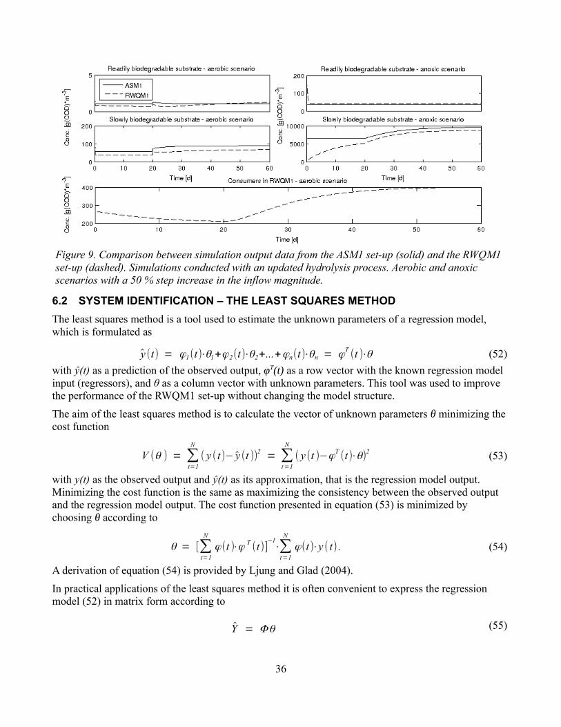
6.2 SYSTEM IDENTIFICATION – THE LEAST SQUARES METHOD

The least squares method is a tool used to estimate the unknown parameters of a regression model, which is formulated as

y (t) = ϕ1(t)⋅θ1+ϕ2(t)⋅θ2+...+ϕn(t)⋅θn = ϕT(t )⋅θ (52)

with ŷ(t) as a prediction of the observed output, φT(t) as a row vector with the known regression model input (regressors), and θ as a column vector with unknown parameters. This tool was used to improve the performance of the RWQM1 set-up without changing the model structure.

The aim of the least squares method is to calculate the vector of unknown parameters θ minimizing the cost function

V (θ ) = ∑t=1

N

( y ( t)− y (t ))2= ∑

t=1

N

( y (t )−ϕT(t)⋅θ)

2 (53)

with y(t) as the observed output and ŷ(t) as its approximation, that is the regression model output. Minimizing the cost function is the same as maximizing the consistency between the observed output and the regression model output. The cost function presented in equation (53) is minimized by choosing θ according to

θ = [∑t=1

N

ϕ(t )⋅ϕ T (t)]−1⋅∑

t=1

N

ϕ(t)⋅y ( t) . (54)

A derivation of equation (54) is provided by Ljung and Glad (2004).

In practical applications of the least squares method it is often convenient to express the regression model (52) in matrix form according to

Y = Φθ (55)

36

Figure 9. Comparison between simulation output data from the ASM1 set-up (solid) and the RWQM1 set-up (dashed). Simulations conducted with an updated hydrolysis process. Aerobic and anoxic scenarios with a 50 % step increase in the inflow magnitude.

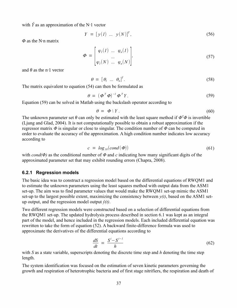
with Ŷ as an approximation of the N·1 vector

Y = [ y (1) ... y (N )]T , (56)

Φ as the N·n matrix

Φ = [ϕ1(1) ... ϕn(1)

...ϕ1(N ) ... ϕn(N )] , (57)

and θ as the n·1 vector

θ = [θ1 ... θn]T . (58)

The matrix equivalent to equation (54) can then be formulated as

θ = (Φ T Φ)−1 Φ T Y . (59)

Equation (59) can be solved in Matlab using the backslash operator according to

θ = Φ \ Y . (60)The unknown parameter set θ can only be estimated with the least square method if ΦTΦ is invertible (Ljung and Glad, 2004). It is not computationally possible to obtain a robust approximation if the regressor matrix Φ is singular or close to singular. The condition number of Φ can be computed in order to evaluate the accuracy of the approximation. A high condition number indicates low accuracy according to

c = log 10(cond (Φ)) (61)

with cond(Φ) as the conditional number of Φ and c indicating how many significant digits of the approximated parameter set that may exhibit rounding errors (Chapra, 2008).

6.2.1 Regression models

The basic idea was to construct a regression model based on the differential equations of RWQM1 and to estimate the unknown parameters using the least squares method with output data from the ASM1 set-up. The aim was to find parameter values that would make the RWQM1 set-up mimic the ASM1 set-up to the largest possible extent, maximizing the consistency between y(t), based on the ASM1 set-up output, and the regression model output ŷ(t).

Two different regression models were constructed based on a selection of differential equations from the RWQM1 set-up. The updated hydrolysis process described in section 6.1 was kept as an integral part of the model, and hence included in the regression models. Each included differential equation was rewritten to take the form of equation (52). A backward finite-difference formula was used to approximate the derivatives of the differential equations according to

dSdt

=S i

−S i−1

h(62)

with S as a state variable, superscripts denoting the discrete time step and h denoting the time step length.

The system identification was focused on the estimation of seven kinetic parameters governing the growth and respiration of heterotrophic bacteria and of first stage nitrifiers, the respiration and death of

37

consumers and the hydrolysis (Table 15). The choice of which parameters to include was strictly limited since the model had to be linear in terms of all included parameters. It was hence not possible to include any stoichiometric parameters or the kinetic parameters that were part of Monod functions. An other limitation was that the unknown parameters had to be chosen so that the regressors became linearly independent in order to make the condition number of the regressor matrix Φ sufficiently low.

Table 15. Parameters estimated with the least squares method

kgro,H,aer kresp,H,aer kgro,N1,aer kresp,N1 kresp,CON kdeath,CON khyd

Notation in regression model θ1 θ2 θ3 θ4 θ5 θ6 θ7

Default value [d-1] 2 0.2 0.8 0.05 0.05 0.05 3

The steps taken to rewrite the differential equation governing the change of readily biodegradable substrate (SS) are described below. The RWQM1 differential equation governing the change of the state variable was defined as

dS S

dt= e1,1⋅p1+e2,1⋅p2+e4,1⋅p4+e5,1⋅p5+e22,1⋅p22+

QV

⋅(S S ,in−S S) (63)

with ei,1 as the stoichiometric coefficient linking process i to state variable 1 (that is SS), pi as process number i, Q as the flow magnitude, V as the basin volume, SS as the concentration of readily biodegradable substrate within the basin and SS,in as the ditto within the inflow. Processes p1, p2, p4, p5

and p22 are presented in equation (35) through equation (38), and in equation (51), respectively. A discretization of equation (63) yields

S St−S S

t−1

h= e1,1⋅p1

t−1+e2,1⋅p2

t−1+e4,1⋅p4

t−1+e5,1⋅p5

t−1+e22,1⋅p22

t−1+

Q t−1

V⋅(S S ,in

t−1−S S

t−1) (64)

with superscripts denoting the discrete time step. Examination of the processes included in equation (64), presented in section 3.3, reveals that the equation contains the two unknown parameters kgro,H,aer and khyd. The processes p1 and p2 represent the aerobic growth of heterotrophs on ammonium and nitrate, respectively. Both of them include the unknown parameter kgro,H,aer. Process p22 represents hydrolysis and it includes the unknown parameter khyd. Multiplying both sides of (64) with the time step length and moving all terms to the left hand side, apart from those containing unknown parameters yields

S St−S S

t−1−h⋅

Qt−1

V⋅(S S , in

t−1−S S

t−1)−h⋅e4,1⋅p4

t−1−h⋅e5,1⋅p5

t−1=

= h⋅e1,1⋅p1t−1

+h⋅e2,1⋅p2t−1

+h⋅e22,1⋅p22t−1.

(65)

For consistency with equation (52) the unknown parameters were explicitly written according to

S St−S S

t−1−h⋅

Qt−1

V⋅(S S , in

t−1−S S

t−1)−h⋅e4,1⋅p4

t−1−h⋅e5,1⋅p5

t−1=

=h

k gro , H ,aer

⋅(e1,1⋅p1t−1

+ e2,1⋅p2t−1

)⋅k gro , H , aer+h

k hyd

⋅e22,1⋅p22t−1

⋅k hyd .(66)

The notation of equation (52) may now be introduced and this is done in equation (67). The parameters kgro,H,aer and khyd in equation (66) represents the unknown parameters θ1 and θ7 in the regression model.

38

All included differential equations were rewritten following the steps above. The derivations are however omitted.

The regression models were made as large as possible in terms of the number of included differential equations, aiming for a least squares method optimizing the unknown parameters with respect to as many state variables as possible. The number of included differential equations was limited by the fact that they had to be defined both in RWQM1 and in ASM1. They had to be defined in RWQM1 since the regression models were to be based on RWQM1 and they had to be defined in ASM1 since the system identification was to be conducted with output data from ASM1. Some state variables of RWQM1 had to be merged in order to obtain consistency. This was the case with the state variables of nitrate and nitrite (SNO3 and SNO2), ammonium and ammonia (SNH3 and SNH2), and first and second stage nitrifiers (XN1 and XN2). Those state variables were merged in order to match the ASM1 state variables of nitrate plus nitrite (SNO), ammonium plus ammonia (SNH) and autotrophic bacteria (XA). Also, the ASM1 state variables of particulate inert organic matter (XI) and particulate products arising from biomass decay (XP) were merged in order to match the RWQM1 state variable of inert particulate matter (XI). The differential equations included in the first regression model were those governing the change of readily and slowly biodegradable substrate (SS and XS), inert particulate organic matter (XI), heterotrophic and autotrophic bacteria (XH and XA), dissolved oxygen (SO2), nitrate plus nitrite (SNO), and ammonium plus ammonia (SNH). That is all differential equations that were defined in both models, except the one governing the change of soluble inert organic matter (SI). This differential equation was not included because the concentration of soluble inert organic matter was unaffected by biochemical processes. The second regression model was extended to include the differential equation governing the change of consumers (XCON). This state variable was not explicitly defined within the ASM1 set-up, it was therefore approximated and the approximation method is presented in sub-section 6.2.2.

The first regression model is presented in equation (67) through (74) and the second is presented in equation (67) through (75). They are hence identical except that the second regression model includes one additional differential equation.

The part of the regression models linked to the change of readily biodegradable substrate (SS) was defined as

ySS(t) = S S

t−SS

t−1−h⋅

Qt−1

V⋅(SS ,in

t−1−S S

t−1)−h⋅e4,1⋅p4

t−1−h⋅e5,1⋅p5

t−1 ,

ϕ1SS

(t) =h

k gro , H ,aer

⋅(e1,1⋅p1t−1

+ e2,1⋅p2t−1

) ,

ϕ7SS( t) =

hk hyd

⋅e22,1⋅p22,t−1

ϕiSS(t ) = 0, i = 2, 3, 4, 5, 6.

(67)

with h as the time step length, ei,j as the stoichiometric coefficient linking process i to state variable j, pi as process number i and t as the discrete sample time. All processes are presented in Appendix D. However, the indexes of equation (67) refer to the process notation of the S-function presented in Appendix E. All stoichiometric coefficients are presented in Appendix C.

The part of the regression models linked to the change of inert particulate organic matter (XI) was defined as

39

y XI(t ) = X I

t−X I

t−1−h⋅

Q t−1

V⋅( X I , in

t−1−X I

t−1)−h⋅(e6,22⋅p6

t−1+e10,22⋅p10

t−1) ,

ϕ2XI(t ) =

hk resp , H ,aer

⋅e3,22⋅p3t−1 ,

ϕ4XI(t ) =

hk resp , N1

⋅e8,22⋅p8t−1 ,

ϕ5XI

(t) =h

k resp ,CON

⋅e20,22⋅p20t−1 ,

ϕ6XI

(t) =h

k death ,CON

⋅e21,22⋅p21t−1 ,

ϕiXI (t) = 0, i = 1, 3, 7.

(68)

The part of the regression models linked to the change of slowly biodegradable substrate (XS) was defined as

y XS(t) = X S

t−X S

t−1−h⋅

Q t−1

V⋅( X S ,in

t−1−X S

t−1)−

−h⋅(e16,21⋅p16t−1

+e17,21⋅p17t−1

+e18,21⋅p18t−1

+e19,21⋅p19t−1

) ,

ϕ6XS

(t ) =h

k death ,CON

⋅e21,21⋅p21t−1 ,

ϕ7XS

( t) =h

k hyd

⋅e22,21⋅p22t−1 ,

ϕiXS

(t) = 0, i = 1, 2, 3, 4, 5.

(69)

The part of the regression models linked to the change of heterotrophic bacteria (XH) was defined as

y XH(t) = X H

t−X H

t−1−h⋅

Qt−1

V⋅( X H ,in

t−1−X H

t−1)−

−h⋅(e4,16⋅p4t−1

+e5,16⋅p5t−1

+e6,16⋅p6t−1

+e17,16⋅p17t−1

) ,

ϕ1XH

(t) =h

k gro , H ,aer

⋅(e1,16⋅p1t−1

+ e2,16⋅p2t−1

) ,

ϕ2XH

(t ) =h

k resp , H ,aer

⋅e3,16⋅p3t−1 ,

ϕiXH

(t) = 0, i = 3, 4, 5, 6, 7.

(70)

The part of the regression models linked to the change of autotrophic bacteria (XA) was defined as

y XA(t) = X N1

t+ X N2

t−X N1

t−1−X N2

t−1−h⋅

Q t−1

V⋅(( X N1 ,in

t−1−X N1

t−1)+(X N2 ,in

t−1−X N2

t−1))−

−h⋅(e9,18⋅p9t−1

+e10,18⋅p10t−1

+e18,17⋅p18t−1

+e19,18⋅p19t−1

) ,

ϕ3XA

(t) =h

k gro , N1 ,aer

⋅e7,17⋅p7t−1 ,

ϕ4XA

(t) =h

kresp , N1

⋅e8,17⋅p8t−1 ,

ϕiXA

(t) = 0, i = 1, 2, 5, 6, 7.

(71)

40

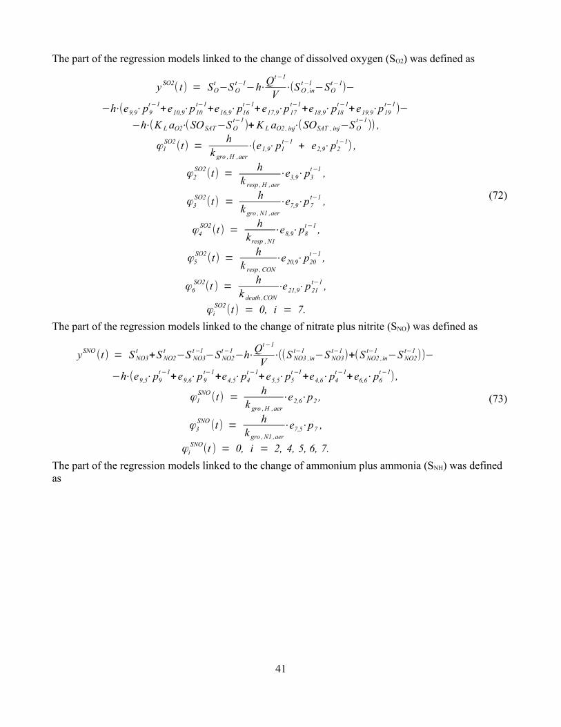
The part of the regression models linked to the change of dissolved oxygen (SO2) was defined as

y SO2( t) = SO

t−S O

t−1−h⋅

Qt−1

V⋅(S O ,in

t−1−SO

t−1)−

−h⋅(e9,9⋅p9t−1

+e10,9⋅p10t−1

+e16,9⋅p16t−1

+e17,9⋅p17t−1

+e18,9⋅p18t−1

+e19,9⋅p19t−1

)−

−h⋅(K L aO2⋅(SOSAT−S Ot−1

)+ K L aO2 , inj⋅(SOSAT , inj−S Ot−1

)) ,

ϕ1SO2

(t) =h

k gro , H ,aer

⋅(e1,9⋅p1t−1

+ e2,9⋅p2t−1

) ,

ϕ2SO2

(t) =h

k resp , H ,aer

⋅e3,9⋅p3t−1 ,

ϕ3SO2

(t) =h

k gro , N1 ,aer

⋅e7,9⋅p7t−1 ,

ϕ4SO2

(t) =h

kresp , N1

⋅e8,9⋅p8t−1 ,

ϕ5SO2

(t) =h

k resp , CON

⋅e20,9⋅p20t−1 ,

ϕ6SO2

(t ) =h

k death ,CON

⋅e21,9⋅p21t−1 ,

ϕiSO2

(t) = 0, i = 7.

(72)

The part of the regression models linked to the change of nitrate plus nitrite (SNO) was defined as

ySNO(t) = S NO3

t+S NO2

t−S NO3

t−1−S NO2

t−1−h⋅

Qt−1

V⋅((S NO3 ,in

t−1−S NO3

t−1)+(S NO2 ,in

t−1−S NO2

t−1))−

−h⋅(e9,5⋅p9t−1

+e9,6⋅p9t−1

+e4,5⋅p4t−1

+e5,5⋅p5t−1

+e4,6⋅p4t−1

+e6,6⋅p6t−1

) ,

ϕ1SNO

(t) =h

k gro , H ,aer

⋅e2,6⋅p2 ,

ϕ3SNO

(t) =h

k gro , N1 ,aer

⋅e7,5⋅p7 ,

ϕiSNO

(t ) = 0, i = 2, 4, 5, 6, 7.

(73)

The part of the regression models linked to the change of ammonium plus ammonia (SNH) was defined as

41

ySNH(t) = S NH4

t+S NH3

t−S NH4

t−1−S NH3

t−1−h⋅

Q t−1

V⋅((S NH4 ,in

t−1−S NH4

t−1)+(S NH3 ,in

t−1−S NH3

t−1))−

−h⋅(e6,3⋅p6t−1

+e10,3⋅p10t−1

+e16,3⋅p16t−1

+e17,3⋅p17t−1

+e18,3⋅p18t−1

+e19,3⋅p19t−1

) ,

ϕ1SNH

(t ) =h

k gro , H , aer

⋅e1,3⋅p1t−1 ,

ϕ2SNH

(t) =h

kresp , H , aer

⋅e3,3⋅p3t−1 ,

ϕ3SNH (t) =

hk gro , N1 ,aer

⋅e7,3⋅p7t−1 ,

ϕ4SNH

(t) =h

k resp , N1

⋅e8,3⋅p8t−1 ,

ϕ5SNH

( t ) =h

k resp , CON

⋅e20,3⋅p20t−1 ,

ϕ6SNH

(t ) =h

k death ,CON

⋅e21,3⋅p21t−1 ,

ϕiSNH

(t) = 0, i = 7.

(74)

The part of the second regression model linked to the change of consumers (XCON) was defined as

y XCON(t) = X H

t−X H

t−1−h⋅

Qt −1

V⋅( X H ,in

t−1−X H

t−1)−

−h⋅(e4,16⋅p4t−1

+e5,16⋅p5t−1

+e6,16⋅p6t−1

+e17,16⋅p17t−1

) ,

ϕ5XCON

(t) =h

k resp ,CON

⋅e20,20⋅p20t−1 ,

ϕ6XCON

(t) =h

k death , CON

⋅e21,20⋅p21t−1 ,

ϕiXCON

(t) = 0, i = 1, 2, 3, 4, 7.

(75)

The different parts of the two regression models as presented in equation (67) through (75) were expressed in matrix form according to

Y i= [ y i

(1) ... y i( N )]

T ,

Φ i= [

ϕ1i(1) ... ϕn

i(1)

...ϕ1

i(N ) ... ϕn

i(N )] ,

i = S S , X I , X S , X H , X A , S O2 , S NO , S NH , X CON ,

(76)

and merged into larger regression models according to

Y = [Y SS Y XI Y XS Y XH Y XA Y SO2 Y SNO Y SNH]T ,

Φ = [Φ SS Φ XI Φ XS Φ XH Φ XA Φ SO2 Φ SNO Φ SNH]T ,

(77)

and

Y = [Y SS Y XI Y XS Y XH Y XA Y SO2 Y SNO Y SNH Y XCON]T ,

Φ = [Φ SS Φ XI Φ XS Φ XH Φ XA Φ SO2 Φ SNO Φ SNH Φ XCON]T ,

(78)

42

respectively. This formulation enabled estimation of the seven unknown parameters presented in Table 15 with respect to the optimization of all included state variables simultaneously.

Both regression models were validated by estimating the unknown parameters presented in Table 15 using equation (60) with input and output data from the RWQM1 set-up. Input and output data were taken from a simulation of the aerobic scenario described in sub-section 5.3.1. A pseudo random binary sequence was applied to the inflow magnitude in order to achieve an excitation of all included state variables (Figure 10).

Both regression models returned parameter values close to the true ones (Table 16). The regressor matrix (Φ) of the first regression model had a condition number of 27, indicating a robust solution. The corresponding value for the second regression model was 26, also indicating a robust solution. Since the parameter approximations were so close to the true parameter values, both proposed regression models were considered correct.

Table 16. Parameter approximations obtained by applying the least squares method to simulation output data from the RWQM1 set-up

kgro,H,aer kresp,H,aer kgro,N1,aer kresp,N1 kresp,CON kdeath,CON khyd

True parameter values 2.0000 0.2000 0.8000 0.0500 0.0500 0.0500 3.0000

First regression model 2.0001 0.2001 0.8000 0.0499 0.0494 0.0504 3.0002

Second regression model 2.0001 0.2001 0.7999 0.0498 0.0495 0.0504 3.0003

6.2.2 Assumptions done to allow usage of the least squares method with simulation data from the ASM1 set-up

Some of the state variables included in the regression models were not defined in the ASM1 set-up. This prohibited a straightforward calculation of the regression model matrices Y and Φ from the ASM1 simulation output. The concerned state variables were SH, SNO3, SNO2, XN1, XN2, SHPO4, SH2PO4 and XCON, from now on referred to as the unknown state variables. In order to conduct the system identification it was necessary to approximate them from other state variables included in the ASM1 set-up. Five assumptions were defined in order to enable such approximations. All assumptions were based on the

43

Figure 10. Magnitude of the inflow to the activated sludge basin equal to the sum of the inflow to the wastewater treatment plant and the sludge recirculation. The inflow to the wastewater treatment plant was described by a pseudo random binary sequence.

output from a simulation of the RWQM1 set-up according to the aerobic scenario described in sub-section 5.3.1, with default parameter values and an inflow magnitude created with the pseudo random binary sequence (Figure 10). A correlation analysis was conducted to investigate the degree of correlation between the unknown state variables and state variables also included in ASM1. One or two regression models were proposed for each unknown state variable, describing its value as a function of one or several known state variables. The regression models were created in Matlab using the regress function according to

[b ,bint , r , rint , stats ] = regress(S 1 , ones (length(S ) , 1) S2 S3 ... S n) (79)

with b as a vector of regression coefficients, bint as the 95 % confidence intervals for b, r as a vector of residuals, rint as a matrix of intervals that can be used to identify outliers, and stats as a vector including the R² statistic, the F statistic, the p value and an estimate of the error variance. The first argument S1 is the dependent variable of the regression model, that is the unknown state variable. The second argument represents the constant term of the regression model and argument S2 to Sn are the independent variables. They were chosen as the state variables also included in ASM1 that were strongly correlated with state variable S1.

1. The concentration of hydrogen was described as a first order function of heterotrophic and autotrophic bacteria according to

S H = 1.2110⋅10−4+2.6236⋅10−6

⋅X A−6.4428⋅10−8⋅X H . (80)

The correlation analysis returned a relatively high correlation between the concentration of hydrogen and the concentration of heterotrophic bacteria (ρ = 0.64), and an even higher correlation between the concentration of hydrogen and the concentration of autotrophic bacteria (ρ = 0.78). All regression coefficient in equation (80) were significant at a significance level of 0.05 and the R2 value of the proposed model was 0.65. Constraints were defined for the regression model application domain according to

0 ⩽ S H ⇔ 0 ⩽ 1.2110⋅10−4+2.6236⋅10−6

⋅X A−6.4428⋅10−8⋅X H ⇔

⇔ 6.4428⋅10−8⋅X H −2.6236⋅10−6

⋅X A ⩽ 1.2110⋅10−4 .(81)

2. Two regression models were proposed describing the concentrations of nitrate and nitrite as first order functions of the total concentration of nitrate plus nitrite according to

S NO3 = −1.2860+1.0258⋅S NO ,S NO2 = 1.2860−0.0258⋅S NO . (82)

The correlation analysis returned a very high correlation between the concentration of nitrate and the total concentration of nitrate plus nitrite (ρ = 1.00), and a high correlation between the concentration of nitrite and the total concentration of nitrate plus nitrite (ρ = 0.90). All regression coefficients of equation (82) were significant at a significance level of 0.05 and the R2 values of the proposed models were 1.00 (nitrate) and 0.82 (nitrite). It was chosen to accept the nitrate regression model since it had the higher R2 value, and to describe the concentration of nitrite as the total concentration of nitrate plus nitrite minus the approximated concentration of nitrate. Constraints were defined for the regression model application domain according to

0 ⩽ S NO3 ⇔ 0 ⩽ −1.2860+1.0258⋅S NO ⇔ 1.2537 ⩽ S NO ,S NO3 ⩽ S NO ⇔ −1.2860+1.0258⋅S NO ⩽ S NO ⇔ S NO ⩽ 43.3333.

(83)

3. Two regression models were proposed describing the concentrations of first and second stage

44

autotrophic nitrifiers as first order functions of the total concentration of autotrophic nitrifiers according to

X N1 = −0.4657+0.8318⋅X A ,X N2=0.4657+0.1682⋅X A . (84)

The correlation analysis returned a very high correlation between the concentration of first stage nitrifiers and the total concentration of nitrifiers (ρ = 1.00), and a very high correlation between the concentration of second stage nitrifiers and the total concentration of nitrifiers (ρ = 0.99). All regression coefficients of equation (84) were significant at a significance level of 0.05 and the R2 values of the proposed models were 1.00 (first stage nitrifiers) and 0.99 (second stage nitrifiers). It was chosen to accept the first stage nitrifiers regression model since it had the higher R2 value, and to describe the concentration of second stage nitrifiers as the total concentration of autotrophic nitrifiers minus the estimated concentration of first stage nitrifiers. Constraints were defined for the regression model application domain according to

0 ⩽ X N1 ⇔ 0 ⩽ −0.4657+0.8318⋅X A ⇔ 0.5599 ⩽ X A. (85)

4. The total concentration of inorganic phosphorous, that is SHPO4 plus SH2PO4, was described as a first order function of nitrate plus nitrite, readily biodegradable substrate and slowly biodegradable substrate according to

S HPO4+S H2PO4 = −1.8602+0.1820⋅S NO+0.0643⋅X S−1.2109⋅S S . (86)

The correlation analysis returned a relatively high correlation between the total concentration of nitrate and nitrite, and the total concentration of inorganic phosphorous (ρ = 0.75), a somewhat lower correlation between the concentration of slowly biodegradable substrate and the total concentration of inorganic phosphorous (ρ = -0.63), and an even lower correlation between the concentration of readily biodegradable substrate and the total concentration of inorganic phosphorous (ρ = -0.59). All regression coefficients of equation (86) were significant at a significance level of 0.05 and the R2 value of the proposed model was 0.71. The concentrations of hydrogen phosphate and dihydrogen phosphate were calculated from the approximated hydrogen concentration and the approximated total concentration of inorganic phosphorous according to equation (50).

5. Two regression models were proposed describing the concentration of consumers. The first one described the concentration as a first order function of the concentration of inert organic matter while the other one described the concentration as a first order function of the concentration of inert organic matter and the total concentration of all substrates that consumers consume according to

X CON = −1.5384⋅102+0.1696⋅X I , (87)

X CON = −1.8679⋅102+0.2136⋅X I−0.0620⋅X sub ,

X sub = X H + X A+ X S .(88)

The correlation analysis returned a high correlation between the concentration of consumers and the concentration of inert organic matter (ρ = 0.95), and a relatively low correlation between the concentration of consumers and the total concentration of all substrates that the consumers consume (ρ = 0.36). All regression coefficients of equation (87) and equation (88) were

45

significant at a significance level of 0.05 and the R2 values of the proposed models were 0.90 (without Xsub) and 1.00 (with Xsub). It was chosen to accept the extended regression model that included Xsub since it had the higher R2 value.

The concentrations of ammonium and ammonia were calculated from the approximated hydrogen concentration and the total concentration of ammonium and ammonia according to equation (44).

6.2.3 Parameter approximations

The least squares method was used together with the two regression models presented in sub-section 6.2.1 in order to approximate the unknown parameters presented in Table 15. As discussed in sub-section 5.3.2 the RWQM1 set-up was unable to describe the production of slowly biodegradable matter in anoxic environments. The system identification was hence only focused on aerobic conditions. Input and output data were taken from a simulation of the ASM1 set-up according to the aerobic scenario described in sub-section 5.3.1. A pseudo random binary sequence was applied to the inflow magnitude in order to achieve an excitation of all included state variables (Figure 10). The unknown parameters were estimated using equation (60), and using the System Identification Toolbox in Matlab. In the System Identification Toolbox lower bounds were applied to the unknown parameters forcing them to take non-negative values.

Application of the unbounded least squares method based on the first regression model presented in sub-section 6.2.1 returned unrealistic parameter values (Table 17). The parameters defining the respiration rate of heterotrophic bacteria, first stage nitrifiers and consumers were assigned negative parameter values. The condition number of the regressor matrix Φ was 119 indicating a relatively robust solution. The proposed regression model reproduced 80 % of the variation in the Y vector. However, Simulink simulations of the RWQM1 set-up based on the approximated parameter set returned unreasonable output data with large negative concentrations in several state variables.

Application of the bounded least squares method (conducted in Matlab's System Identification Toolbox) based on the first regression model presented in sub-section 6.2.1 returned a parameter set similar to the parameter set obtained in the unbounded application (Table 17). The main difference was that the three negative parameters were set to zero. The proposed regression model reproduced 64 % of the variation in the Y vector. Simulink simulations of the RWQM1 set-up based on the approximated parameter set returned reasonable output data without negative concentrations. The model performance was increased in terms of inert organic matter and ammonium plus ammonia, relatively unaffected in terms of heterotrophic bacteria, and decreased in terms of readily biodegradable substrate and consumers (Figure 11).

Table 17. Parameter approximations obtained by applying the least squares method based on the first regression model presented in sub-section 6.2.1 on simulation output data from the ASM1 set-up

Method kgro,H,aer kresp,H,aer kgro,N1,aer kresp,N1 kresp,CON kdeath,CON khyd

Unbounded 0.4815 -0.1053 0.3607 -0.3218 -0.0844 1.5243 2.2305

Bounded 0.4813 0 0.3189 0 0 1.4676 2.2219

46

Application of the unbounded least squares method based on the second (extended) regression model presented in sub-section 6.2.1 returned unrealistic parameter values (Table 18). The major difference from the parameter set obtained with the unbounded method based on the first regression model was that the kinetic parameter governing the respiration rate of consumers was decreased from -0.0844 to -0.7622. The condition number of the regressor matrix Φ was 117 indicating a relatively robust solution. The proposed regression model reproduced 80 % of the variation in the Y vector. Simulink simulations of the RWQM1 set-up based on the approximated parameter set returned reasonable output data without negative concentrations. The model performance was increased as compared to simulations with the default parameter set in terms of ammonium plus ammonia, slowly biodegradable substrate, heterotrophic bacteria and autotrophic bacteria, relatively unaffected in terms of dissolved oxygen and inert organic matter, and decreased in terms of nitrate plus nitrite and readily biodegradable substrate (Figure 12 and Figure 13). The concentration of consumers was well above zero throughout the simulation.

Application of the bounded least squares method (conducted in Matlab's System Identification Toolbox) based on the second (extended) regression model presented in sub-section 6.2.1 returned a parameter set similar to the parameter set obtained in the unbounded application (Table 18). The main difference was that the three negative parameters were set to zero. The proposed regression model reproduced 60 % of the variation in the Y vector. Simulink simulations of the RWQM1 set-up based on the approximated parameter set returned reasonable output data without negative concentrations. However, the concentration of consumers decreased to zero.

47

Figure 11. Comparison between simulation output data from the ASM1 set-up (solid) and the RWQM1 set-up simulated with the default parameter set (dashed) and the updated parameter set based on the bounded system identification conducted with the first regression model (dotted).

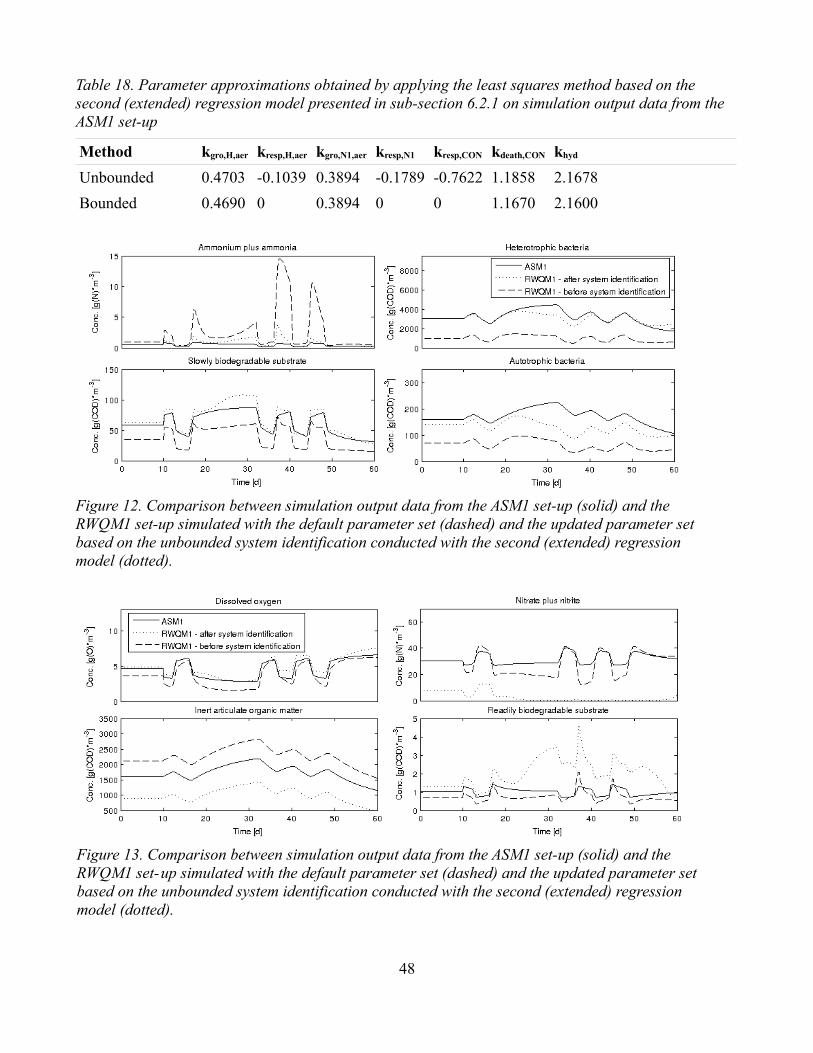
Table 18. Parameter approximations obtained by applying the least squares method based on the second (extended) regression model presented in sub-section 6.2.1 on simulation output data from the ASM1 set-up

Method kgro,H,aer kresp,H,aer kgro,N1,aer kresp,N1 kresp,CON kdeath,CON khyd

Unbounded 0.4703 -0.1039 0.3894 -0.1789 -0.7622 1.1858 2.1678

Bounded 0.4690 0 0.3894 0 0 1.1670 2.1600

48

Figure 12. Comparison between simulation output data from the ASM1 set-up (solid) and the RWQM1 set-up simulated with the default parameter set (dashed) and the updated parameter set based on the unbounded system identification conducted with the second (extended) regression model (dotted).

Figure 13. Comparison between simulation output data from the ASM1 set-up (solid) and the RWQM1 set-up simulated with the default parameter set (dashed) and the updated parameter set based on the unbounded system identification conducted with the second (extended) regression model (dotted).

6.2.4 Evaluation of assumptions

In order to investigate to what extent the assumptions presented in sub-section 6.2.2 affected the results of the system identification an alternative set of assumptions was defined. It was in particular considered important to investigate if an alternative set of assumptions could yield a non-negative parameter approximation. The new assumptions were not based on output data from the RWQM1 set-up. They were instead defined to cover a broad spectrum of theoretically possible relationships between the unknown state variables and state variables included in ASM1. Several different assumptions were defined for each unknown state variable resulting in a large amount of possible assumption combinations.

1. The hydrogen concentration was either described as a constant value corresponding to pH 7, or as a first order function of heterotrophic and autotrophic bacteria according to equation (80).

2. The concentration of nitrate was set to a fraction of the total concentration of nitrate plus nitrite equal to 0.5, 0.75, 0.9 or 0.99. The nitrite concentration was set equal to the remaining fraction.

3. The concentration of first stage nitrifiers was set to a fraction of the total concentration of nitrifiers equal to 0.5, 0.75, 0.9 or 0.99. The concentration of second stage nitrifiers was set equal to the remaining fraction.

4. The total concentration of inorganic phosphorous was set to 10 g(P)·m-3 in order to make sure that no processes were phosphorous limited. The concentrations of hydrogen phosphate and dihydrogen phosphate were calculated from the approximated hydrogen concentration and the total concentration of inorganic phosphorous according to equation (50).

5. The concentration of consumers was set to a fraction of the concentration of inert organic matter or as a fraction of the concentration of all substrates that consumers consume. The fractions were set equal to 0.01, 0.1, 0.25 or 0.5.

The concentrations of ammonium and ammonia was, as before, calculated from the approximated hydrogen concentration and the total concentration of ammonium plus ammonia according to equation (44).

All combinations of the above presented assumptions were evaluated by applying the least squares method based on the second (extended) regression model presented in sub-section 6.2.1 on simulation output data from the ASM1 set-up. Input and output data were taken from a simulation of an aerobic scenario as described in sub-section 5.3.1. A pseudo random binary sequence was applied to the inflow magnitude in order to achieve an excitation of all included state variables (Figure 10). The evaluation showed that the assumptions affected the approximated parameter values to a large extent and that all included combinations yielded parameter sets with at least one negative parameter value.

6.3 SYSTEM IDENTIFICATION – NON-LINEAR PROGRAMMING

Non-linear system identification was, just like the least squares method, applied aiming to improve the RWQM1 set-up without changing the model structure. The Matlab function fmincon was used to minimize a cost function based on the relative error presented in equation (89). It was focused on the same seven kinetic parameters and the same nine state variables as was the least squares method based on the second (extended) regression model. As stated in sub-section 6.2.2, ASM1 does not include a state variable for the concentration of consumers. This concentration was therefore estimated according to equation (88). The updated hydrolysis process presented in section 6.1 was kept as an integral part of

49

the model. Lower bounds were applied to all unknown parameters so that they only could take non-negative values. The identification was conducted on data from an aerobic scenario as described in sub-section 5.3.1.

The cost function was defined as

V (θ ) = ∑i=1

N

∑j=1

J

erel2 ,

erel =y sim ,asm1

j( i)− ysim , rwqm1

j(i)

ysim , asm1j

(i),

i = 1, 2, ... N ,

(89)

with j denoting the state variable (SS, XI, XS, XH, XA, SO2, SNO, SNH and XCON) and i denoting the discrete time step. Defining the cost function as a function of the relative error rather than the absolute error made all state variables equally important. A cost function based on the absolute error would optimize the unknown parameter set with respect to the strongest signals, for example inert organic matter and heterotrophic bacteria, at the expense of weaker signals such as readily biodegradable substrate and dissolved oxygen. A discussion on how the relative error may be used in linear system identification is provided by Tofallis (2007).

The non-linear system identification was initially aimed at finding parameter values that would optimize the model performance at steady state. Both the ASM1 set-up and the RWQM1 set-up were simulated over 1 000 days using constant influent data as described in section 5.2. Only the last 500 days were used in the cost function to ensure that all transients were excluded. The initial guess was set equal to the default parameter values presented in Table 15.

It was found that the non-linear system identification improved the model performance in terms of a cost function decrease from 260 with the default parameter values to 46 with the estimated parameter set (Table 20). The improvement was apparent in all state variables except inert organic matter and nitrate plus nitrite (Table 19).

50

Table 19. Steady state values under aerobic conditions according to the ASM1 set-up and the RWQM1 set-up with default and estimated parameter values

State variable RWQM1 – default parameter values

RWQM1 – estimated parameter set

ASM1 Unit

Readily biodegradable substrate

0.68 0.77 1.0 [g(COD)·m-3]

Inert organic matter 2100 2100 2300 [g(COD)·m-3]

Slowly biodegradable substrate

35 59 59 [g(COD)·m-3]

Heterotrophic bacteria 990 1500 3000 [g(COD)·m-3]

Autotrophic bacteria 69 110 160 [g(COD)·m-3]

Dissolved oxygen 3.7 4.0 4.7 [g(O)·m-3]

Nitrate plus nitrite 30 28 30 [g(N)·m-3]

Ammonium plus ammonia 0.91 0.47 0.48 [g(N)·m-3]

Consumers 200 98 110 a [g(COD)·m-3]a Calculated according to equation (88).

The estimated parameter set from the initial non-linear system identification was used as an initial guess in a new non-linear system identification aimed at optimizing the model performance over a step increase in the inflow magnitude. Both models were simulated over 1 300 days and the inflow magnitude was increased by a step of 25 % after 1 000 days.

It was found that the second non-linear system identification improved the model performance in terms of a cost function decrease from 126 with the parameter values from the initial non-linear system identification to 82 with the new estimated parameter set (Table 20). Altogether the model performance was improved in terms of most state variables, for example those representing autotrophic bacteria, heterotrophic bacteria and consumers (Figure 14). However, the model performance was decreased in terms of the state variables representing nitrate plus nitrite and particulate inert organic matter (Figure 14).

Table 20. Parameter sets estimated in the first and the second non-linear system identification

Method kgro,H,aer kresp,H,aer kgro,N1,aer kresp,N1 kresp,CON kdeath,CON khyd

Non-linear system identification aimed at steady state values

1.0896 0.1294 0.6488 0.0340 0.0177 0.1871 1.7512

Non-linear system identification aimed at system dynamics

1.0763 0.1522 0.7767 0.0026 0.0421 0.1452 1.8785

51

52

Figure 14. Comparison between simulation output data from the ASM1 set-up (solid) and the RWQM1 set-up simulated with the default parameter set (dashed) and the updated parameter set based on the second non-linear system identification (dotted). The ASM1 concentration of consumers was calculated according to equation (88).

7 INTRODUCING ALGAE DYNAMICS

7.1 DEVELOPMENT OF PROCESSES DESCRIBING ALGAL GROWTH

Processes describing algal growth were by default included in RWQM1 and they are presented in equation (39) and (40). These processes were defined to describe the algae dynamics of a river system. It was considered unlikely that they would describe the algae dynamics of an activated sludge process accurately because of the differences between the systems. Therefore, an alternative description of algal growth was developed based on the theory presented in section 2.2. The main structure of the original processes describing algal growth in RWQM1 was kept in order to avoid changes in the stoichiometric matrix. Hence, algal growth was divided into two processes, growth on ammonium and growth on nitrate. Both processes were defined as functions of temperature, pH and several limiting substrates presented later in this section. The relationship between algal growth and temperature was described according to the default process description of RWQM1 using the same parameter values. The relationship between algal growth and pH or limiting substrates were described by Monod functions.

Reichert et al. (2001) described the relationship between algal growth and inorganic nitrogen as, inter alia, a Monod function of ammonium and ammonia. This description was not incorporated into the new process description since plant uptake of nitrogen is considered to be targeted at either nitrate or ammonium, not ammonia (Campbell and Reece, 2008). The Monod functions relating algal growth to the availability of inorganic nitrogen were instead taken from Sah et al. (2011). The Monod function for algal growth on ammonium was defined as

S NH4

K NH4 , ALG+S NH4(90)

while the corresponding function for growth on nitrate was defined as

S NO3

K NO3, ALG+S NO3

⋅K NH4 , ALG

K NH4 , ALG+S NH4

. (91)

The parameter values KNH4,ALG and KNO3,ALG were both set to 0.01 g(N)·m-3 following Sah et al. (2011).

The Monod function relating algal growth to the availability of inorganic phosphorous was defined as

S HPO4+S H2PO4

K PO4 , ALG+S HPO4+S H2PO4(92)

following the default process description of RWQM1. The half saturation coefficient KPO4,ALG was set to 0.01 g(P)·m-3 following Beran and Kargi (2005).

The Monod function relating algal growth to the availability of carbon dioxide was defined as

SCO2

KCO2 , ALG+S CO2(93)

following Decostere et al. (2013), Yang (2011), Banks et al. (2003), Mashauri and Kayombo (2002), Carberry and Greene (1992) and Buhr and Miller (1983). The half saturation coefficient KCO2,ALG was set to 0.055 g(C)·m-3 following Decostere et al. (2013). Their study was focused on carbon dioxide dynamics and their model was shown to function well.

The Monod function relating algal growth to pH was defined as

53

K pH , ALG

K pH , ALG+ y ( pH ),

y ( pH ) = 10∣optpH ALG−pH ∣−1

(94)

following Beran and Kargi (2005) and Mashauri and Kayombo (2002). The half saturation parameter KpH,ALG was set to 170 and the parameter optpHALG was set to 7.45, in both cases the mean of the parameter values used by Beran and Kargi (2005) and Mashauri and Kayombo (2002).

The maximum specific growth rate kgro,ALG was set to 2 d-1 following the default process description of RWQM1. This value can be compared to the corresponding parameter values used in the models presented in section 2.2, which varied between 0.48 d-1 and 2.55 d-1 (Table 1).

Considering the combined effect of temperature, pH and all limiting substrates the process describing algal growth on ammonium was defined as

dX A

dt= k gro , ALG⋅eβALG⋅(T −T 0)⋅

K pH

K pH + y ( pH )⋅

⋅S NH4

K N , ALG+S NH4

⋅S HPO4+S H2PO4

K PO4 , ALG+S HPO4+S H2PO4

⋅S CO2

K CO2+SCO2

⋅X ALG

(95)

while the corresponding process for algal growth on nitrate was defined as

dX A

dt= k gro , ALG⋅eβALG⋅(T −T 0)⋅

K pH

K pH + y ( pH )⋅

⋅S NO3

K N , ALG+S NO3

⋅K N , ALG

K N , ALG+S NH4

⋅S HPO4+S H2PO4

K PO4 , ALG+S HPO4+S H2PO4

⋅SCO2

KCO2+S CO2

⋅X ALG .(96)

It should be noticed that the models presented in section 2.2 vary a lot in terms of structure and parameter values. A major reason is the variation in application domain. This elucidates the importance of model verification. The model presented in equation (95) and equation (96) should therefore preferably be evaluated against observed data from the specific system that it is supposed to describe. It should also be investigated if a division between algal growth on bicarbonate and algal growth on carbon dioxide, as proposed by Decostere et al. (2013), would increase the model performance.

According to equation (95) and (96) phosphorous and nitrogen may simultaneously limit the growth process. However, plant growth is only limited by one substrate at any one time instant, a fact referred to as Liebig's Law of Minimum (Ågren and Andersson, 2009). Liebig's Law of Minimum was included in the models proposed by Beran and Kargi (2005) and Carberry and Greene (1992) as presented in section 2.2. However, according to Ågren and Andersson (2009) Liebig's Law of Minimum should only include nutrients, not light intensity as in the proposed models. Liebig's Law of Minimum was not included in equation (95) and (96) for consistency with the other process descriptions within the RWQM1 set-up.

7.2 INCORPORATION OF ALGAE DYNAMICS INTO THE ACTIVATED SLUDGE MODEL BASED ON THE RIVER WATER QUALITY MODEL NO. 1

The processes describing algal growth as presented in equation (95) and (96) were incorporated into two different versions of the RWQM1 set-up. The first version was based on the default RWQM1 parameter values as presented in Table 15 while the other version was based on the parameter set obtained in the second non-linear system identification presented in Table 20. Both versions included

54

the updated hydrolysis process described in section 6.1. It was investigated how the introduction of algae affected the system dynamics of an activated sludge process without aeration and without carbon dioxide injection, described by the first scenario of section 5.1.

Both versions of the RWQM1 set-up were initially simulated without algae. It was found that the concentrations of autotrophic bacteria and consumers reached zero due to the low dissolved oxygen concentrations (Table 21). Introducing algae into the two model versions affected the system dynamics in terms of most state variables (Table 21). Two distinct changes were found in the increased dissolved oxygen concentration and the decreased carbon dioxide concentration. Both changes were expected as a result of algal photosynthesis. The carbon dioxide concentration was decreased from 20 g(C)·m-3 to 12 g(C)·m-3 with default parameter values, or to 13 g(C)·m-3 with parameter values from the non-linear system identification. The new concentrations were still well above the water-atmosphere saturation value of 0.11 g(C)·m-3 and also above the carbon dioxide injection saturation value of 11.7 g(C)·m-3. The increase of dissolved oxygen enabled a stable population of consumers that in turn made the concentrations of heterotrophic bacteria and slowly biodegradable substrate decrease through predation and consumption. The concentration of autotrophic bacteria reached zero even though the oxygen concentration increased, most likely a consequence of the high predation rate.

Table 21. Steady-state values of some state variables from simulations with and without algae

State variable Default parameter set - no algae

Updated parameter set - no algae

Default parameter set - with algae

Updated parameter set - with algae

Unit

Readily biodegradable substrate

69 69 32 69 [g(COD)·m-3]

Slowly biodegradable substrate

6300 6300 1000 1200 [g(COD)·m-3]

Inert organic matter 1600 1600 3000 3600 [g(COD)·m-3]

Dissolved oxygen 0.00013 0.00024 0.37 0.68 [g(O)·m-3]

Carbon dioxide 20 20 12 13 [g(C)·m-3]

Heterotrophic bacteria 890 890 44 37 [g(COD)·m-3]

Autotrophic bacteria 0 0 0 0 [g(COD)·m-3]

Consumers 0 0 4000 2900 [g(COD)·m-3]

Algae 0 0 930 1100 [g(COD)·m-3]

All particulate matter a 8800 8800 9000 8800 [g(COD)·m-3]

pH 7.0 7.0 7.2 7.2 [-]a XH+XA+XALG+XCON+XS+XI, calculated from the rounded values presented in the table.

55

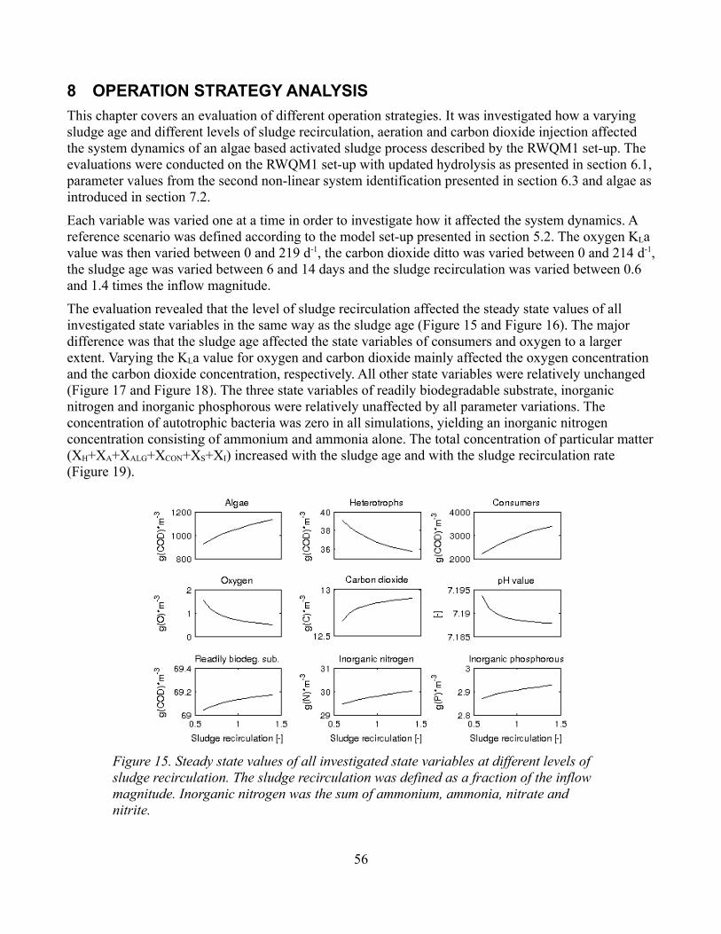
8 OPERATION STRATEGY ANALYSIS

This chapter covers an evaluation of different operation strategies. It was investigated how a varying sludge age and different levels of sludge recirculation, aeration and carbon dioxide injection affected the system dynamics of an algae based activated sludge process described by the RWQM1 set-up. The evaluations were conducted on the RWQM1 set-up with updated hydrolysis as presented in section 6.1, parameter values from the second non-linear system identification presented in section 6.3 and algae as introduced in section 7.2.

Each variable was varied one at a time in order to investigate how it affected the system dynamics. A reference scenario was defined according to the model set-up presented in section 5.2. The oxygen KLa value was then varied between 0 and 219 d-1, the carbon dioxide ditto was varied between 0 and 214 d-1, the sludge age was varied between 6 and 14 days and the sludge recirculation was varied between 0.6 and 1.4 times the inflow magnitude.

The evaluation revealed that the level of sludge recirculation affected the steady state values of all investigated state variables in the same way as the sludge age (Figure 15 and Figure 16). The major difference was that the sludge age affected the state variables of consumers and oxygen to a larger extent. Varying the KLa value for oxygen and carbon dioxide mainly affected the oxygen concentration and the carbon dioxide concentration, respectively. All other state variables were relatively unchanged (Figure 17 and Figure 18). The three state variables of readily biodegradable substrate, inorganic nitrogen and inorganic phosphorous were relatively unaffected by all parameter variations. The concentration of autotrophic bacteria was zero in all simulations, yielding an inorganic nitrogen concentration consisting of ammonium and ammonia alone. The total concentration of particular matter (XH+XA+XALG+XCON+XS+XI) increased with the sludge age and with the sludge recirculation rate (Figure 19).

56

Figure 15. Steady state values of all investigated state variables at different levels of sludge recirculation. The sludge recirculation was defined as a fraction of the inflow magnitude. Inorganic nitrogen was the sum of ammonium, ammonia, nitrate and nitrite.

57

Figure 16. Steady state values of all investigated state variables at different sludge ages. Inorganic nitrogen was the sum of ammonium, ammonia, nitrate and nitrite.

Figure 17. Steady state values of all investigated state variables at different levels of aeration. Inorganic nitrogen was the sum of ammonium, ammonia, nitrate and nitrite.

58

Figure 18. Steady state values of all investigated state variables at different levels of carbon dioxide injection. Inorganic nitrogen was the sum of ammonium, ammonia, nitrate and nitrite.

Figure 19. Steady state values of the total concentration of particulate matter (XH+XA+XALG+XCON+XS+XI) as a function of sludge recirculation and sludge age.

9 ALTERNATIVE SEDIMENTATION CONFIGURATION

The original sedimentation unit was modelled assuming ideal sedimentation, as stated in section 5.2. All particulate matter was hence assumed to settle, including zoo-plankton (consumers). This assumption does not agree with the theory presented by Moreno-Grau et al. (1996) who modelled zoo-plankton as mobile. Their approach was considered interesting and reasonable. It was therefore investigated how different sedimentation rates of zoo-plankton affected the system dynamics of the RWQM1 set-up evaluated in chapter 8. Ideal sedimentation was assumed for all other particulate matter.

It was found that the sedimentation configuration affected the steady state values of all investigated state variables rather much (Table 22). A sedimentation rate of 80 % or less resulted in a consumer concentration so low that the autotrophic bacteria persisted predation. Sedimentation rates lower than 100 % yielded unreasonably high oxygen concentrations. This was probably a consequence of high algae concentrations relative the concentrations of oxygen consuming bacteria and consumers.

Table 22. Steady state values of simulations with different levels of zoo-plankton settling

State variable Unit 100 % 95 % 90 % 80 % 0 %

Slowly biodegradable substrate [g(COD)·m-3] 1200 1500 1800 230 78

Inert organic matter [g(COD)·m-3] 3600 3200 3600 5800 6800

Heterotrophic bacteria [g(COD)·m-3] 37 68 400 2300 3400

Autotrophic bacteria [g(COD)·m-3] 0 0 0 52 340

Consumers [g(COD)·m-3] 2900 1200 580 200 0

Algae [g(COD)·m-3] 1100 1400 2300 4900 6000

All particulate matter a [g(COD)·m-3] 8800 7400 8700 13000 17000

Readily biodegradable substrate [g(COD)·m-3] 69 69 62 2.3 0.72

Ammonium plus ammonia [g(N)·m-3] 30 25 24 0.74 0.098

Nitrate plus nitrite [g(N)·m-3] 0 0 0 17 18

Inorganic phosphorous [g(P)·m-3] 2.9 2.1 1.8 0.46 0.078

Dissolved oxygen [g(O)·m-3] 0.68 68 96 81 91

Carbon dioxide [g(C)·m-3] 13 0.27 0.076 0.031 0.022

pH [-] 7.2 8.7 9.2 9.3 9.4a Calculated from the rounded values presented in the table.

59

10 DISCUSSION

10.1 EFFLUENT QUALITY AND CONSUMERS

The results of the operation strategy analysis presented in chapter 8 indicate that the proposed model describes a system that fails in its purpose to enhance water quality. The effluent concentrations of inorganic nitrogen, inorganic phosphorous and readily biodegradable substrate were close to the influent concentrations of 31.56 g(N)·m-3, 3.2 g(P)·m-3 and 69.5 g(COD)·m-3, respectively, irrespective of operation strategy (Figure 15 through Figure 18). Lower effluent concentrations of both nutrients and readily biodegradable substrate were obtained with a lower sedimentation rate of consumers (zoo-plankton), as presented in chapter 9. However, a lower sedimentation rate also yielded unreasonably high concentrations of dissolved oxygen, indicating an incorrect model description.

A relatively high consumer concentration varying between about 1 800 g(COD)·m-3 and 4 000 g(COD)·m-3 was obtained in the operation strategy analysis presented in chapter 8. This concentration can be compared to the concentration of algae varying between about 625 g(COD)·m-3 and 1 250 g(COD)·m-3. These concentrations and the ratio between them should be evaluated against measurement data. It seems likely that the concentration of consumers is unreasonably high.

The low quality of the calibration process discussed in section 10.4 undermines the results presented in chapter 8 and chapter 9. These results should therefore be regarded as examples of how the model may be used after further development rather than accurate system descriptions.

10.2 MODEL STRUCTURE

The model structure of RWQM1 was considered suitable for the modelling of wastewater treatment. It was, just like ASM1, summarized in a Gujer matrix and the extensive usage of ASM1 indicates a wide acceptance of the Gujer matrix in wastewater treatment modelling. The processes of RWQM1 were, even though developed to describe a river system, considered suitable for the modelling of wastewater treatment. The processes coupled to hydrolysis and algal growth were adjusted within this study, and it is likely that some further adjustments are needed in order to make the model describe an algae based activated sludge process more accurately. It might for example be a good idea to include a decay process in which bacteria are transformed into slowly biodegradable substrate. However, the original structure was considered a very good starting point for future modelling.

10.3 LIGHT INTENSITY

The effect of light intensity on algal growth was neglected in this study. It was reasoned that the light intensity at the light source can be kept constant in large scale indoor applications. However, if the light intensity is allowed to vary the model must be adjusted to account for light intensity dependence since such variations affect algal growth rather much (Wu et al., 2013). Adjusting the model to account for light intensity dependence can be done through the introduction of a light intensity limiting factor as discussed in sub-section 2.2.1.

10.4 CALIBRATION

A central part of this study was to adjust the RWQM1 set-up presented in chapter 5 aiming for consistency with the ASM1 set-up presented in chapter 4. This was done through adjustments of the

60

hydrolysis process and the calibration of seven kinetic parameters through linear and non-linear system identification, as presented in chapter 6. The calibration process improved the model performance somewhat. However, it was considered insufficient and four shortcomings were identified as crucial.

The first shortcoming was attributed to the small number of parameters included in the calibration process. RWQM1 includes 23 state variables and 30 processes which can be compared to the eight state variables and 13 processes included in ASM1. The number of model parameters of RWQM1 is hence relatively large: 13 stoichiometric parameters and 49 kinetic parameters linked to biological processes. Apart from those, it is necessary to define the elemental mass fractions of the nine organic state variables in order to enable calculation of the stoichiometric coefficients. The large model size and the consequent model complexity aggravates calibration. The seven kinetic parameters that were included in the calibration process were considered insufficient. A central obstacle is that the stoichiometric coefficients are calculated outside the main program, they were downloaded from Peter Reichert's homepage (Reichert, 2014). This makes it difficult to include stoichiometric parameters and elemental mass fractions in any system identification method. It was not possible to extend the linear system identification to include any additional parameters, as discussed in sub-section 6.2.1. However, the non-linear system identification may be extended with kinetic parameters, even those that are included in Monod functions.

The second shortcoming was attributed to the small number of state variables included in the calibration process. Only nine out of 23 state variables were included in the second linear system identification and in the non-linear system identification. It was not possible to include any additional state variables due to the lack of measurement data.

The third shortcoming was attributed to the calibration approach. All unknown parameters were estimated simultaneously through linear or non-linear system identification. This approach aggravates the usage of system knowledge that is crucial in the development of conceptual models. An alternative method would be to parametrize one parameter at a time based on laboratory experiments. Henze et al. (1987) provide information about how to determine both stoichiometric and kinetic parameters in this way. They specify which parameters that are unnecessary to calibrate due to low variation in parameter values between different reactors, and which parameters that are crucial to parametrize thoroughly. The elemental mass fractions should preferably be defined based on laboratory experiments on the sludge that will be used in the subject activated sludge plant. It is likely that the elemental mass fractions of organic state variables in a wastewater differ from those in a river system.

The fourth and last crucial shortcoming of the calibration process was attributed to the absence of algae. It must be emphasized that the developed model was supposed to describe an activated sludge basin in which algae was to constitute an important function. However, the calibration was conducted on a system without algae.

10.5 FURTHER RESEARCH

A more comprehensive study should be focused on the gas exchange processes presented in section 2.3. Literature values of KLa vary rather much (Table 2 and Table 3) depending on application domain. It is hence important to estimate the KLa values from studies on an activated sludge basin. The unreasonably high oxygen concentrations obtained in simulations presented in chapter 9 indicate that the gas exchange description of the proposed model is insufficient. This elucidates the need for KLa studies targeted on systems subject to extensive photosynthesis. The saturation value for carbon dioxide injection calculated in this study should also be reviewed. This value is dependent on several factors

61

such as the carbon dioxide concentration of the injection gas and the carbon dioxide concentration of the gas bubbles just before they reach the surface. Each unique carbon dioxide injection application is hence associated with a unique saturation value.

The quality of the influent data should be improved through a study focused on the characteristics of raw sewage. The influent data used in this study was not well substantiated and this was due to the lack of documentation. Hence et al. (1987) provide information on how to determine the state variables included in ASM1. RWQM1 includes several state variables usually not included in wastewater treatment models. Raw sewage concentrations of those state variables are hence not well documented.

10.6 RELATED RESEARCH

This thesis was aimed at the modelling of an algae based activated sludge process. The proposed model should be regarded as a tool for future use in control and operation strategy analyses. Several alternative models have been proposed in literature. For example the one presented by Ifrim et al. (2014) and those presented in section 2.2. The relatively large number of models aimed at the modelling of algae based wastewater treatment composes a good base for future model development.

Algae cultivation may be used in fields of application other than that of wastewater treatment targeted at nutrient and COD removal. Research has for example been targeted at algae based food production (Becker, 2003), heavy metal removal (Doshi, Seth, Ray and Kothari, 2008) and biofuel production (Kong et al., 2010; Wang, 2013). The different fields of application may be combined in order to obtain cost effective solutions. An example is the combination of wastewater treatment and biofuel production discussed by Kong et al. (2010). Knowledge gained in one field of application may be utilized in the others and collaboration between the different fields will likely result in more sustainable solutions.

62

11 CONCLUSIONS

The overall aim of this thesis was reached in that a model describing the dynamics of an algae based activated sludge process was proposed and evaluated.

The calibration process conducted within this study consisted of a linear and a non-linear system identification. The non-linear system identification improved the model performance of the proposed model somewhat. However, the calibration process was considered insufficient. The major obstacle was the lack of comprehensive measurement data from a real algae based activated sludge process. Without such data and without the proper system understanding it was not possible to calibrate and evaluate the proposed model set-up satisfactory.

It was shown that the modelled algae based activated sludge process failed in its purpose to reduce the concentration of nutrients and of readily biodegradable substrate. It was also shown that the removal of both nutrients and readily biodegradable substrate was enhanced by assuming that the consumers (zoo-plankton) are mobile. Those results clearly indicate that a better system understanding is needed in order to describe the system accurately.

The model structure of RWQM1 was considered a suitable starting point for the modelling of an algae based activated sludge process. It includes all state variables needed to describe algae dynamics and pH dynamics. Also, the model structure allows a straightforward application to an activated sludge environment.

Future work should be targeted at further model development and this work will require better data and a more comprehensive system understanding.

63

12 REFERENCES

Ackerman, S.A. and Knox, J.A., 2003. Meteorology - Understanding the Atmosphere. Canada: Thomson Learning, Inc.

Ågren, G.I. and Andersson, F.O., 2009. Terrestrial Ecosystem Science: theoretical and empirical approaches and their applications. Course materials.

Alex, J., Benedetti, L., Copp, J., Gernaey, K., Jeppsson, U., Nopens, I., Pons, M.-N., Rosen, C., Steyer, J.-P. and Vanrolleghem, P., 2008a. Benchmark Simulation Model no. 1. [online] IWA Task Group. Available at: <http://www.iea.lth.se/WWTmodels_download/>.

Alex, J., Benedetti, L., Copp, J., Gernaey, K.V., Jeppsson, U., Nopens, I., Pons, M.-N., Rieger, L., Rosen, C., Steyer, J.P., Vanrolleghem, P. and Winkler, S., 2008b. Benchmark Simulation Model no. 1 (BSM1). [online] Department of Industrial Electrical Engineering and Automation, Lund University. Available at: <https://www.iea.lth.se/publications/Reports/LTH-IEA-7229.pdf>.

Atkins, P. and Jones, L., 2008. Chemical principles: the quest for insight. New York: W.H. Freeman.

Banks, C.J., Koloskov, G.B., Lock, A.C. and Heaven, S., 2003. A computer simulation of the oxygen balance in a cold climate winter storage WSP during the critical spring warm-up period. Water science and technology: a journal of the International Association on Water Pollution Research, 48(2), pp.189–196.

Becker, W., 2003. Microalgae in Human and Animal Nutrition. In: A. Richmond, ed., Handbook of Microalgal Culture. [online] Blackwell Publishing Ltd, pp.312–351. Available at: <http://onlinelibrary.wiley.com/doi/10.1002/9780470995280.ch18/summary> [Accessed 19 May 2014].

Beran, B. and Kargi, F., 2005. A dynamic mathematical model for wastewater stabilization ponds. Ecological Modelling, 181(1), pp.39–57.

Bernes, C. and Lundgren, L.J., 2009. Bruk och missbruk av naturens resurser: en svensk miljöhistoria. Monitor. Stockholm: Naturvårdsverket.

Buhr, H.O. and Miller, S.B., 1983. A Dynamic Model of the High-Rate Algal-Bacterial Wastewater Treatment Pond. Water Research, 17(1), pp.29–37.

Burks, B.D. and Minnis, M.M., 1994. Onsite wastewater treatment systems. Madison, WI: Hogarth House.

Campbell, N.A. and Reece, J.B., 2008. Biology. 8th ed. San Francisco: Pearson Education, Inc.

Carberry, J.B. and Greene, R.W., 1992. Model of algal bacterial clay wastewater treatment system. Water Science & Technology, 26(7/8), pp.1697–1706.

Chapra, S.C., 2008. Applied Numerical Methods with Matlab - for Engineers and Scientists. 2nd ed. New York: McGraw-Hill.

64

Chapra, S.C., 2011. Rubbish, Stink, and Death: The Historical Evolution, Present State, and Future Direction of Water-Quality Management and Modeling. Environmental Engineering Research, 16(3), pp.113–119.

Colomer, F.L. and Rico, D.P., 1993. Mechanistic model for facultative stabilization ponds. Water Environment Research, 65(5), pp.679–685.

Decostere, B., Janssens, N., Alvarado, A., Maere, T., Goethals, P., Van Hulle, S.W.H. and Nopens, I., 2013. A combined respirometer–titrimeter for the determination of microalgae kinetics: Experimental data collection and modelling. Chemical Engineering Journal, 222, pp.85–93.

Dlugokencky, E. and Tans, P., 2014. Trends in Atmospheric Carbon dioxide. Available at: <www.esrl.noaa.gov/gmd/ccgg/trends/> [Accessed 1 Apr. 2014].

Dochain, D., Grégoire, S., Pauss, A. and Schaegger, M., 2003. Dynamical modelling of a waste stabilisation pond. Bioprocess and biosystems engineering, 26(1), pp.19–26.

Doshi, H., Seth, C., Ray, A. and Kothari, I.L., 2008. Bioaccumulation of Heavy Metals by Green Algae. Current Microbiology, 56(3), pp.246–255.

Drever, J.I., 1997. The geochemistry of natural waters: surface and groundwater environments. Upper Saddle River, N.J.: Prentice Hall.

Henze, M., Grady, C.P.L.J., Gujer, W., Marais, G. v. R. and Matsuo, T., 1987. Activated Sludge Model No. 1. IAWPRC Scientific and Technical Report No. 1. London: IAWPRC.

Henze, M., Gujer, W., Mino, T., Matsuo, T., Wentzel, M.C. and Marais, G. v. R., 1995. Activated Sludge Model No. 2. IAWQ Scientific and Technical Report No. 3. [online] London: IAWQ, p.36. Available at: <http://search.proquest.com.ezproxy.its.uu.se/science/docview/13634445/B83F15BAE4A44053PQ/1?accountid=14715> [Accessed 2 Apr. 2014].

Hoffmann, J.P., 1998. Wastewater treatment with suspended and nonsuspended algae. Journal of Phycology, 34(5), pp.757–763.

Ifrim, G.A., Titica, M., Cogne, G., Boillereaux, L., Legrand, J. and Caraman, S., 2014. Dynamic pH model for autotrophic growth of microalgae in photobioreactor: A tool for monitoring and control purposes. AIChE Journal, 60(2), pp.585–599.

Jorgensen, S.E., Mejer, H. and Friis, M., 1978. Examination of a Lake Model. Ecological Modelling, 4(2-3), pp.253–278.

Kong, Q., Li, L., Martinez, B., Chen, P. and Ruan, R., 2010. Culture of Microalgae Chlamydomonas reinhardtii in Wastewater for Biomass Feedstock Production. Applied Biochemistry and Biotechnology, 160(1), pp.9–18.

Ljung, L. and Glad, T., 2004. Modellbygge och simulering. 2:5 ed. Lund: Studentlitteratur AB.

Mashauri, D.A. and Kayombo, S., 2002. Application of the two coupled models for water quality

65

management: facultative pond cum constructed wetland models. Physics and Chemistry of the Earth, 27(11–22), pp.773–781.

Mesplé, F., Casellas, C., Troussellier, M. and Bontoux, J., 1996. Modelling Orthophosphate Evolution in a High Rate Algal Pond. Ecological Modelling, 89(1), pp.13–21.

Moreno-Grau, S., Garcia-Sanchez, A., Moreno-Clavel, J., Serrano-Aniorte, J. and Moreno-Grau, M.D., 1996. A mathematical model for waste water stabilization ponds with macrophytes and microphytes. Ecological Modelling, 91(1-3), pp.77–103.

Noüe, J. de la, Laliberté, G. and Proulx, D., 1992. Algae and waste water. Journal of Applied Phycology, 4, pp.247–254.

Reichert, P., 2014. Eawag. [Homepage] Peter Reichert. Available at: <http://www.eawag.ch/about/personen/homepages/reichert/index> [Accessed 2 Apr. 2014].

Reichert, P., Borchardt, D., Henze, M., Rauch, W., Shanahan, P., Somlyody, L. and Vanrolleghem, P., 2001. River Water Quality Model No. 1 (RWQM1): II. Biochemical process equations. Water Science and Technology, 43(5), pp.11–30.

Reichert, P. and Schuwirth, N., 2010. A generic framework for deriving process stoichiometry in environmental models. Environmental Modelling & Software, 25(10), pp.1241–1251.

Sah, L., Rousseau, D.P.L., Hooijmans, C.M. and Lens, P.N.L., 2011. 3D model for a secondary facultative pond. Ecological Modelling, 222(9), pp.1592–1603.

Svenskt Vatten, 2010. Avloppsteknik 2 - Reningsprocessen. Stockholm: Svenskt Vatten AB.

Tofallis, C., 2007. Least Squares Percentage Regression. [Working paper] Hatfield: University of Hertfordshire. Available at: <http://uhra.herts.ac.uk/handle/2299/965> [Accessed 15 May 2014].

Wang, Y., 2013. Microalgae as the Third Generation Biofuel: Production, Usage, Challenges and Prospects. [online] Available at: <http://www.diva-portal.org/smash/record.jsf?searchId=1&pid=diva2:665095> [Accessed 19 May 2014].

Wu, Y.-H., Li, X., Yu, Y., Hu, H.-Y., Zhang, T.-Y. and Li, F.-M., 2013. An integrated microalgal growth model and its application to optimize the biomass production of Scenedesmus sp. LX1 in open pond under the nutrient level of domestic secondary effluent. Bioresource technology, 144, pp.445–451.

Yang, A., 2011. Modeling and Evaluation of CO2 Supply and Utilization in Algal Ponds. Industrial & Engineering Chemistry Research, [online] 50(19). Available at: <http://dx.doi.org/10.1021/ie200723w> [Accessed 25 Mar. 2014].

66

APPENDIX A – GUJER MATRIX SUMMARIZING THE ACTIVATED SLUDGE MODEL NO. 1 a

a Taken from Henze et al. (1987).

67

APPENDIX B – GUJER MATRIX SUMMARIZING THE RIVER WATER QUALITY MODEL NO. 1 a

a Taken from Reichert et al. (2001).

68

APPENDIX C – STOICHIOMETRIC COEFFICIENTS USED IN APPLICATIONS OF THE RIVER WATER QUALITY MODEL NO. 1 a

i \ j 1 2 3 4 5 6 7 8 9 10 11 12 13 14 15 16 17 18 19 20 21 22 23

1 -1.85 -0.01 -0.01 -0.85 0.27 0.00 1.00

2 -1.85 -0.01 -0.01 -0.80 0.27 0.00 1.00

3 0.07 0.02 -0.77 0.25 0.00 -1.00 0.23

4 -2.22 1.07 -1.07 -0.01 0.39 0.00 1.00

5 -3.71 -1.63 0.00 0.86 -0.12 1.00

6 0.07 -0.27 0.02 0.25 -0.02 -1.00 0.23

7 -4.78 4.70 -0.02 -15.13 -0.32 0.68 1.00

8 0.07 0.02 -0.77 0.25 0.00 -1.00 0.23

9 -20.71 20.63 -0.02 -22.33 -0.32 -0.01 1.00

10 0.07 0.02 -0.77 0.25 0.00 -1.00 0.23

11 -0.06 -0.01 1.00 -0.39 0.00 1.00

12 -0.06 -0.01 1.29 -0.39 -0.01 1.00

13 0.06 0.01 -0.60 0.26 0.00 -1.00 0.40

14 0.03 0.00 0.20 0.00 0.00 -1.00 0.95 0.25

15 0.13 0.02 -0.15 0.32 -0.01 -5.00 1.00 3.85

16 0.13 0.02 -4.77 1.45 -0.01 1.00 -5.77

17 0.45 0.13 -3.80 1.18 -0.02 -8.65 1.00 3.85

18 0.45 0.13 -3.80 1.18 -0.02 -8.65 1.00 3.85

19 0.45 0.13 -3.80 1.18 -0.02 -8.65 1.00 3.85

20 0.06 0.01 -0.60 0.26 0.00 -1.00 0.40

21 0.03 0.00 0.20 0.00 0.00 -1.00 0.95 0.25

22 1.00 0.00 0.00 0.00 0.00 0.00 -1.00

23 -1.00 1.00 0.08

24 -1.00 1.00 0.08

25 1.00 1.00

26 -1.00 1.00 0.07

27 1.00 -1.00 0.03

28 0.30 1.00

29 -1.00 1.00

30 1.00 -1.00

a Downloaded from Peter Reichert's homepage (Reichert, 2014).

69

APPENDIX D – PROCESS RATES OF THE RIVER WATER QUALITY MODEL NO. 1 a

70

a Taken from Reichert et al. (2001).

71

APPENDIX E – S-FUNCTION DESCRIBING THE DIFFERENTIAL EQUATIONS OF THE RIVER WATER QUALITY MODEL NO. 1

function rwqm1(block)% Level-2 MATLAB file S-function describing RWQM1.% Author: Rasmus Pierong% Latest edited: 2014-01-07 setup(block); % end rwqm1 function setup(block) %% Register number of dialog parameters block.NumDialogPrms = 10; % XINIT, par_stoichiometry, par_kinetics, VOL, SO_SAT_inj, SCO2_SAT_inj, SO_SAT, SCO2_SAT, KLa_O2, KLa_CO2 %% Register number of input and output ports block.NumInputPorts = 1; block.NumOutputPorts = 1; %% Setup functional port properties to dynamically %% inherited. block.SetPreCompInpPortInfoToDynamic; block.SetPreCompOutPortInfoToDynamic; block.InputPort(1).Dimensions = 26; % influent quality [23 state variables Q KLa_O2 KLa_CO2] block.InputPort(1).DirectFeedthrough = true; % direct feedthrough of Q block.OutputPort(1).Dimensions = 24; % effluent quality [23 state variables Q] %% Set block sample time to continuous block.SampleTimes = [0 0]; %% Setup Dwork block.NumContStates = 23; % one per state variable %% Set the block simStateCompliance to default (i.e. same as a built-in block) block.SimStateCompliance = 'DefaultSimState'; %% Register methods block.RegBlockMethod('InitializeConditions', @InitConditions); block.RegBlockMethod('Outputs', @Output); block.RegBlockMethod('Derivatives', @Derivative); % end setup function InitConditions(block) %% Initialize Dwork block.ContStates.Data = block.DialogPrm(1).Data(1:23); % [S_S S_I S_NH4 S_NH3

72

S_NO2 S_NO3 S_HPO4 S_H2PO4 S_O2 S_CO2 S_HCO3 S_CO3 S_H S_OH S_Ca X_H X_N1 X_N2 X_ALG X_CON X_S X_I X_P]; % end InitConditions function Output(block) %% Define output parameters block.OutputPort(1).Data(1:23) = block.ContStates.Data; % the 23 state variables block.OutputPort(1).Data(24) = block.InputPort(1).Data(24); % outflow % end Output function Derivative(block) %% Define parameters % Tank volume V = block.DialogPrm(4).Data(1); % Aeration or gas injection KLa_O2_inj = block.InputPort(1).Data(25); KLa_CO2_inj = block.InputPort(1).Data(26); SO_SAT_inj = block.DialogPrm(5).Data; % this value should be equal to the water-atmosphere gas exchange saturation value SCO2_SAT_inj = block.DialogPrm(6).Data; % this value should be higher than the water-atmosphere ditto since the CO2 concentration is higher in the injection gas than in the atmosphere % Water-atmosphere gas exchange KLa_O2 = block.DialogPrm(9).Data; KLa_CO2 = block.DialogPrm(10).Data; SO_SAT = block.DialogPrm(7).Data; SCO2_SAT = block.DialogPrm(8).Data; % Stoichiometric parameters following Reichert et al. (2001) - from % Excel sheet e = block.DialogPrm(2).Data; par_kinetics = block.DialogPrm(3).Data; % Kinetic parameters following Reichert et al. (2001) [K_eq_w K_eq_1 K_eq_2 K_eq_N K_eq_P K_eq_s0 ... T T_0 k_death_ALG k_death_CON k_gro_ALG k_gro_CON k_gro_H_aer k_gro_H_anox k_gro_N1 k_gro_N2 k_hyd ... k_resp_ALG k_resp_CON k_resp_H_aer k_resp_H_anox k_resp_N1 k_resp_N2 ... k_eq_1 k_eq_2 k_eq_w k_eq_N k_eq_P k_eq_s0 k_ads k_des ... K_HPO4_ALG K_HPO4_H_aer K_HPO4_H_anox K_HPO4_N1 K_HPO4_N2 K_N_ALG K_NH4_ALG K_N_H_aer ... K_NH4_N1 K_NO3_H_anox K_NO2_H_anox K_NO2_N2 K_O2_ALG K_O2_CON K_O2_H_aer K_O2_H_anox ... K_O2_N1 K_O2_N2 K_S_H_aer K_S_H_anox ... beta_ALG beta_CON beta_H beta_hyd beta_N1 beta_N2] = deal(par_kinetics{:}); %% Influent quality Q = block.InputPort(1).Data(24);

73

S_Si = block.InputPort(1).Data(1); S_Ii = block.InputPort(1).Data(2); S_NH4i = block.InputPort(1).Data(3); S_NH3i = block.InputPort(1).Data(4); S_NO2i = block.InputPort(1).Data(5); S_NO3i = block.InputPort(1).Data(6); S_HPO4i = block.InputPort(1).Data(7); S_H2PO4i = block.InputPort(1).Data(8); S_O2i = block.InputPort(1).Data(9); S_CO2i = block.InputPort(1).Data(10); S_HCO3i = block.InputPort(1).Data(11); S_CO3i = block.InputPort(1).Data(12); S_Hi = block.InputPort(1).Data(13); S_OHi = block.InputPort(1).Data(14); S_Cai = block.InputPort(1).Data(15); X_Hi = block.InputPort(1).Data(16); X_N1i = block.InputPort(1).Data(17); X_N2i = block.InputPort(1).Data(18); X_ALGi = block.InputPort(1).Data(19); X_CONi = block.InputPort(1).Data(20); X_Si = block.InputPort(1).Data(21); X_Ii = block.InputPort(1).Data(22); X_Pi = block.InputPort(1).Data(23); inflow = [S_Si S_Ii S_NH4i S_NH3i S_NO2i S_NO3i S_HPO4i S_H2PO4i S_O2i S_CO2i S_HCO3i S_CO3i S_Hi S_OHi S_Cai X_Hi X_N1i X_N2i X_ALGi X_CONi X_Si X_Ii X_Pi]'; %% Rename state variables (current values in the basin) S_S = block.ContStates.Data(1); S_I = block.ContStates.Data(2); S_NH4 = block.ContStates.Data(3); S_NH3 = block.ContStates.Data(4); S_NO2 = block.ContStates.Data(5); S_NO3 = block.ContStates.Data(6); S_HPO4 = block.ContStates.Data(7); S_H2PO4 = block.ContStates.Data(8); S_O2 = block.ContStates.Data(9); S_CO2 = block.ContStates.Data(10); S_HCO3 = block.ContStates.Data(11); S_CO3 = block.ContStates.Data(12); S_H = block.ContStates.Data(13); S_OH = block.ContStates.Data(14); S_Ca = block.ContStates.Data(15); X_H = block.ContStates.Data(16); X_N1 = block.ContStates.Data(17); X_N2 = block.ContStates.Data(18); X_ALG = block.ContStates.Data(19); X_CON = block.ContStates.Data(20); X_S = block.ContStates.Data(21); X_I = block.ContStates.Data(22); X_P = block.ContStates.Data(23); statevar = [S_S S_I S_NH4 S_NH3 S_NO2 S_NO3 S_HPO4 S_H2PO4 S_O2 S_CO2 S_HCO3 S_CO3 ...

74

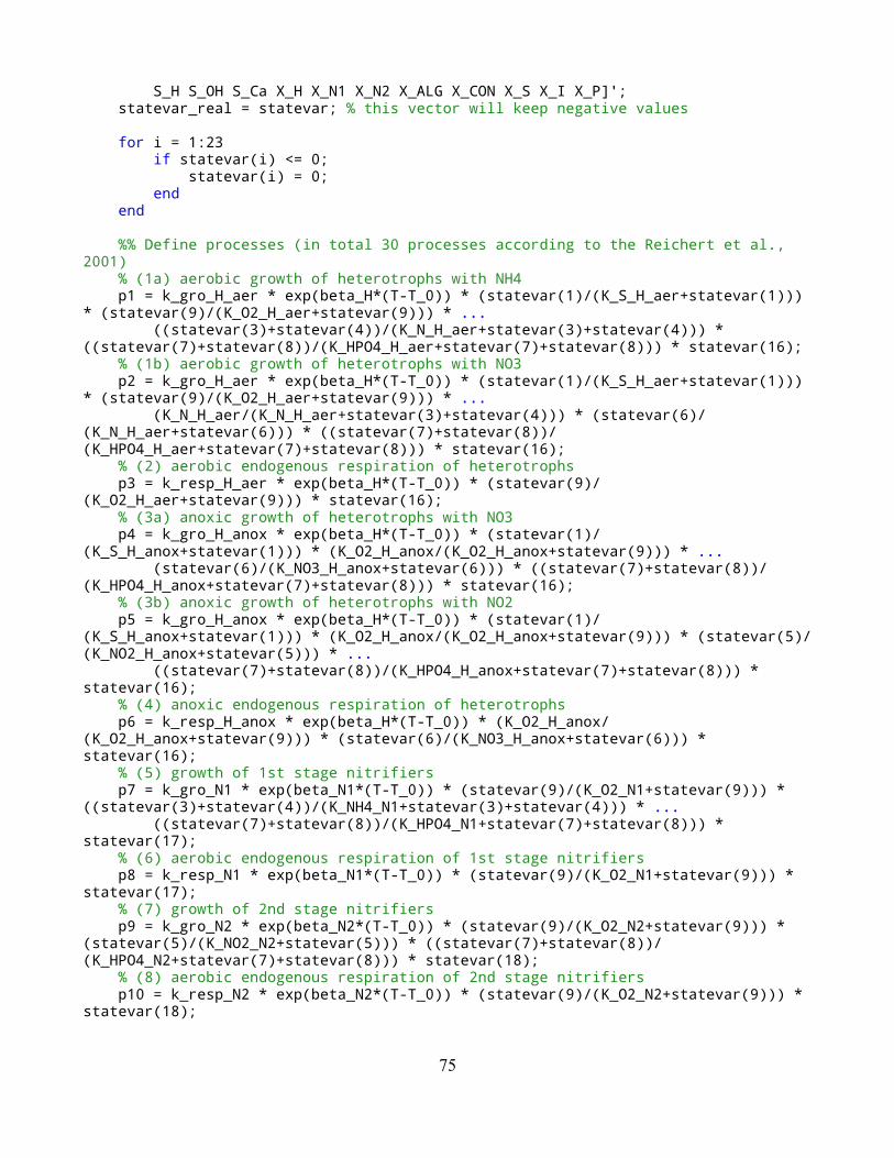
S_H S_OH S_Ca X_H X_N1 X_N2 X_ALG X_CON X_S X_I X_P]'; statevar_real = statevar; % this vector will keep negative values for i = 1:23 if statevar(i) <= 0; statevar(i) = 0; end end %% Define processes (in total 30 processes according to the Reichert et al., 2001) % (1a) aerobic growth of heterotrophs with NH4 p1 = k_gro_H_aer * exp(beta_H*(T-T_0)) * (statevar(1)/(K_S_H_aer+statevar(1))) * (statevar(9)/(K_O2_H_aer+statevar(9))) * ... ((statevar(3)+statevar(4))/(K_N_H_aer+statevar(3)+statevar(4))) * ((statevar(7)+statevar(8))/(K_HPO4_H_aer+statevar(7)+statevar(8))) * statevar(16); % (1b) aerobic growth of heterotrophs with NO3 p2 = k_gro_H_aer * exp(beta_H*(T-T_0)) * (statevar(1)/(K_S_H_aer+statevar(1))) * (statevar(9)/(K_O2_H_aer+statevar(9))) * ... (K_N_H_aer/(K_N_H_aer+statevar(3)+statevar(4))) * (statevar(6)/(K_N_H_aer+statevar(6))) * ((statevar(7)+statevar(8))/(K_HPO4_H_aer+statevar(7)+statevar(8))) * statevar(16); % (2) aerobic endogenous respiration of heterotrophs p3 = k_resp_H_aer * exp(beta_H*(T-T_0)) * (statevar(9)/(K_O2_H_aer+statevar(9))) * statevar(16); % (3a) anoxic growth of heterotrophs with NO3 p4 = k_gro_H_anox * exp(beta_H*(T-T_0)) * (statevar(1)/(K_S_H_anox+statevar(1))) * (K_O2_H_anox/(K_O2_H_anox+statevar(9))) * ... (statevar(6)/(K_NO3_H_anox+statevar(6))) * ((statevar(7)+statevar(8))/(K_HPO4_H_anox+statevar(7)+statevar(8))) * statevar(16); % (3b) anoxic growth of heterotrophs with NO2 p5 = k_gro_H_anox * exp(beta_H*(T-T_0)) * (statevar(1)/(K_S_H_anox+statevar(1))) * (K_O2_H_anox/(K_O2_H_anox+statevar(9))) * (statevar(5)/(K_NO2_H_anox+statevar(5))) * ... ((statevar(7)+statevar(8))/(K_HPO4_H_anox+statevar(7)+statevar(8))) * statevar(16); % (4) anoxic endogenous respiration of heterotrophs p6 = k_resp_H_anox * exp(beta_H*(T-T_0)) * (K_O2_H_anox/(K_O2_H_anox+statevar(9))) * (statevar(6)/(K_NO3_H_anox+statevar(6))) * statevar(16); % (5) growth of 1st stage nitrifiers p7 = k_gro_N1 * exp(beta_N1*(T-T_0)) * (statevar(9)/(K_O2_N1+statevar(9))) * ((statevar(3)+statevar(4))/(K_NH4_N1+statevar(3)+statevar(4))) * ... ((statevar(7)+statevar(8))/(K_HPO4_N1+statevar(7)+statevar(8))) * statevar(17); % (6) aerobic endogenous respiration of 1st stage nitrifiers p8 = k_resp_N1 * exp(beta_N1*(T-T_0)) * (statevar(9)/(K_O2_N1+statevar(9))) * statevar(17); % (7) growth of 2nd stage nitrifiers p9 = k_gro_N2 * exp(beta_N2*(T-T_0)) * (statevar(9)/(K_O2_N2+statevar(9))) * (statevar(5)/(K_NO2_N2+statevar(5))) * ((statevar(7)+statevar(8))/(K_HPO4_N2+statevar(7)+statevar(8))) * statevar(18); % (8) aerobic endogenous respiration of 2nd stage nitrifiers p10 = k_resp_N2 * exp(beta_N2*(T-T_0)) * (statevar(9)/(K_O2_N2+statevar(9))) * statevar(18);

75

% (9a) growth of algae with NH4 p11 = k_gro_ALG * exp(beta_ALG*(T-T_0)) * ((statevar(3)+statevar(4)+statevar(6))/(K_N_ALG+statevar(3)+statevar(4)+statevar(6))) * ... ((statevar(3)+statevar(4))/(K_N_ALG+statevar(3)+statevar(4))) * ((statevar(7)+statevar(8))/(K_HPO4_ALG+statevar(7)+statevar(8))) * statevar(19); % (9b) growth of algae with NO3 p12 = k_gro_ALG * exp(beta_ALG*(T-T_0)) * ((statevar(3)+statevar(4)+statevar(6))/(K_N_ALG+statevar(3)+statevar(4)+statevar(6))) * ((K_NH4_ALG)/(K_NH4_ALG+statevar(3)+statevar(4))) * ... ((statevar(7)+statevar(8))/(K_HPO4_ALG+statevar(7)+statevar(8))) * statevar(19); % (10) aerobic endogenous respiration of algae p13 = k_resp_ALG * exp(beta_ALG*(T-T_0)) * (statevar(9)/(K_O2_ALG+statevar(9))) * statevar(19); % (11) death of algae p14 = k_death_ALG * exp(beta_ALG*(T-T_0)) * statevar(19); % (12a) growth of consumers on algae p15 = k_gro_CON * exp(beta_CON*(T-T_0)) * (statevar(9)/(K_O2_CON+statevar(9))) * statevar(19) * statevar(20); % (12b) growth of consumers on substrate p16 = k_gro_CON * exp(beta_CON*(T-T_0)) * (statevar(9)/(K_O2_CON+statevar(9))) * statevar(21) * statevar(20); % (12c) growth of consumers on heterotrophs p17 = k_gro_CON * exp(beta_CON*(T-T_0)) * (statevar(9)/(K_O2_CON+statevar(9))) * statevar(16) * statevar(20); % (12d) growth of consumers on 1st stage nitrifiers p18 = k_gro_CON * exp(beta_CON*(T-T_0)) * (statevar(9)/(K_O2_CON+statevar(9))) * statevar(17) * statevar(20); % (12e) growth of consumers on 2nd stage nitrifiers p19 = k_gro_CON * exp(beta_CON*(T-T_0)) * (statevar(9)/(K_O2_CON+statevar(9))) * statevar(18) * statevar(20); % (13) aerobic endogenous respiration of consumers p20 = k_resp_CON * exp(beta_CON*(T-T_0)) * (statevar(9)/(K_O2_CON+statevar(9))) * statevar(20); % (14) death of consumers p21 = k_death_CON * exp(beta_CON*(T-T_0)) * statevar(20); % (15) hydrolysis p22 = k_hyd * exp(beta_hyd*(T-T_0)) * statevar(21); % (16) CO2 - HCO3 equilibrium p23 = k_eq_1 * (statevar(10)-statevar(13)*statevar(11)/K_eq_1); % (17) HCO3 - CO3 equilibrium p24 = k_eq_2 * (statevar(11)-statevar(13)*statevar(12)/K_eq_2); % (18) H - OH equilibrium p25 = k_eq_w * (1-statevar(13)*statevar(14)/K_eq_w); % (19) NH4 - NH3 equilibrium p26 = k_eq_N * (statevar(3)-statevar(13)*statevar(4)/K_eq_N); % (20) H2PO4 - HPO4 equilibrium p27 = k_eq_P * (statevar(8)-statevar(13)*statevar(7)/K_eq_P); % (21) Ca - CO3 equilibrium p28 = k_eq_s0 * (1-statevar(15)*statevar(12)/K_eq_s0); % (22) adsorption of phosphate **** not in use **** p29 = k_ads * statevar(7); % (23) desorption of phosphate **** not in use ****

76

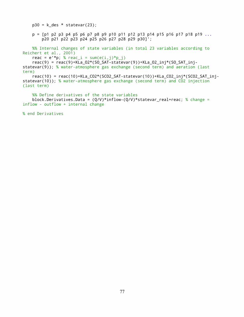
p30 = k_des * statevar(23); p = [p1 p2 p3 p4 p5 p6 p7 p8 p9 p10 p11 p12 p13 p14 p15 p16 p17 p18 p19 ... p20 p21 p22 p23 p24 p25 p26 p27 p28 p29 p30]'; %% Internal changes of state variables (in total 23 variables according to Reichert et al., 2001) reac = e'*p; % reac_i = sum(e(i,j)*p_j) reac(9) = reac(9)+KLa_O2*(SO_SAT-statevar(9))+KLa_O2_inj*(SO_SAT_inj-statevar(9)); % water-atmosphere gas exchange (second term) and aeration (last term) reac(10) = reac(10)+KLa_CO2*(SCO2_SAT-statevar(10))+KLa_CO2_inj*(SCO2_SAT_inj-statevar(10)); % water-atmosphere gas exchange (second term) and CO2 injection (last term) %% Define derivatives of the state variables block.Derivatives.Data = (Q/V)*inflow-(Q/V)*statevar_real+reac; % change = inflow - outflow + internal change % end Derivatives

77