
Modelling Hermetic Compressors Using Different … · Modelling Hermetic Compressors Using...
12
Modelling Hermetic Compressors Using Different Constraint Equations to … J. of the Braz. Soc. of Mech. Sci. & Eng. Copyright © 2009 by ABCM January-March 2009, Vol. XXXI, No. 1 / 35 Edgar A. Estupiñan [email protected] Ilmar F. Santos Senior Member, ABCM [email protected] Technical University of Denmark Department of Mechanical Engineering Nils Koppels Allé, Building 404, DK-2800 Kgs. Lyngby, Denmark Modelling Hermetic Compressors Using Different Constraint Equations to Accommodate Multibody Dynamics and Hydrodynamic Lubrication In this work, the steps involved for the modelling of a reciprocating linear compressor are described in detail. The dynamics of the mechanical components are described with the help of multibody dynamics (rigid components) and finite elements method (flexible components). Some of the mechanical elements are supported by fluid film bearings, where the hydrodynamic interaction forces are described by the Reynolds equation. The system of nonlinear equations is numerically solved for three different restrictive conditions of the motion of the crank, where the third case takes into account lateral and tilting oscillations of the extremity of the crankshaft. The numerical results of the behaviour of the journal bearings for each case are presented giving some insights into design parameters such as, maximum oil film pressure, minimum oil film thickness, maximum vibration levels and dynamic reaction forces among machine components, looking for the optimization and application of active lubrication towards vibration reduction. Keywords: hermetic compressor, multibody dynamics, journal bearing, Reynolds equation, hydrodynamic lubrication. Introduction 1 One of the most common types of compressors used in the refrigeration field is the piston compressor, also known as reciprocating compressor. Small-scale hermetic reciprocating compressors are widely used to compress coolant gas in household refrigerators and air-conditioners. It was at the beginning of the Sixties when these small machines became a household appliance of common use in the industrialized countries. Since then, numerous research studies have been carried out in order to optimize the design and to improve the thermal and mechanical efficiency of refrigeration compressors. Positive displacement compressors mechanically drive the refrigerant gas from the evaporator at low- pressure side to the condenser at high-pressure side, reducing the compressor chamber volume. Reciprocating compressors use pistons that are driven directly through a slider-crank mechanism, converting the rotating movement of the rotor to an oscillating motion. A hermetic reciprocating compressor is a particular case where motor and compressor are directly coupled on the same shaft and contained within the same housing (welded steel shell) and in contact with the refrigerant and oil (Rigola, 2002). A picture and a schematic draw of a hermetic reciprocating compressor used in household refrigerators are shown in Fig.1. Figure 1. Picture and schematic draw of a hermetic reciprocating compressor. Paper accepted December, 2008. Technical Editor: Domingos A. Rade. The study and optimization of the dynamic behaviour of reciprocating compressors, taking in account the hydrodynamics of bearings, are of significant importance for the development of new prototypes. The performance of the bearings affects key functions such as durability and noise and vibration behaviour of the compressor. Optimization studies of the performance of journal bearings by means of numerical simulation may reduce development costs for prototype testing work significantly. Several studies that involve numerical studies and computational models for the analysis of small reciprocating compressors are found in the literature, as it can be seen in the works carried out by Rasmussen (1997) and Rigola (2002). In some studies, numerical simulations of the refrigerant flow through the valves and inside the cylinder during the compression cycle have been included (Longo and Gasparella, 2003), whereas in others the focus has been on the dynamics of motion in steady and transient conditions (Dufour, et al., 1995). Some researchers have included the coupling of fluid- structure dynamics in order to particularly analyse the dynamics of the piston (Gommed and Etsion, 1993; Cho and Moon, 2005). In a study carried out by Kim and Han (2004), an analytical model of the coupled dynamic behaviour of the piston and crankshaft was developed and comparisons between a finite bearing model and a short bearing approach were included. In the same study, a numerical procedure that combines Newton-Raphson method and the successive over relaxation scheme was also presented. In the study carried out by Cho and Moon (2005), a time-incremental numerical algorithm to solve a finite differences model for the estimation of the oil film pressure was coupled with a finite element model for the computation of the structural deformation of the piston. As it is described here, many of the research studies related to compressor modelling are mainly focused on the study of the thermal and fluid dynamic behaviour. In contrast, the main focus of the present work is on the developing of a multibody dynamic model of a hermetic compressor, where the dynamics of the fluid film bearings and the flexibility of the crankshaft are included. The multibody dynamic model, which includes the main mechanical components of the hermetic compressor, is coupled with a finite elements model of the rotor and the hydrodynamic interaction forces, which are computed using analytical solutions of the Reynolds equation. The influence of the crankshaft tilting oscillations on design parameters, such as the minimum film
Transcript of Modelling Hermetic Compressors Using Different … · Modelling Hermetic Compressors Using...
Modelling Hermetic Compressors Using Different Constraint Equations to …
J. of the Braz. Soc. of Mech. Sci. & Eng. Copyright © 2009 by ABCM January-March 2009, Vol. XXXI, No. 1 / 35
Edgar A. Estupiñan [email protected]
Ilmar F. Santos Senior Member, ABCM
[email protected] Technical University of Denmark
Department of Mechanical Engineering Nils Koppels Allé, Building 404, DK-2800
Kgs. Lyngby, Denmark
Modelling Hermetic Compressors Using Different Constraint Equations to Accommodate Multibody Dynamics and Hydrodynamic Lubrication In this work, the steps involved for the modelling of a reciprocating linear compressor are described in detail. The dynamics of the mechanical components are described with the help of multibody dynamics (rigid components) and finite elements method (flexible components). Some of the mechanical elements are supported by fluid film bearings, where the hydrodynamic interaction forces are described by the Reynolds equation. The system of nonlinear equations is numerically solved for three different restrictive conditions of the motion of the crank, where the third case takes into account lateral and tilting oscillations of the extremity of the crankshaft. The numerical results of the behaviour of the journal bearings for each case are presented giving some insights into design parameters such as, maximum oil film pressure, minimum oil film thickness, maximum vibration levels and dynamic reaction forces among machine components, looking for the optimization and application of active lubrication towards vibration reduction. Keywords: hermetic compressor, multibody dynamics, journal bearing, Reynolds equation, hydrodynamic lubrication.
Introduction 1One of the most common types of compressors used in the
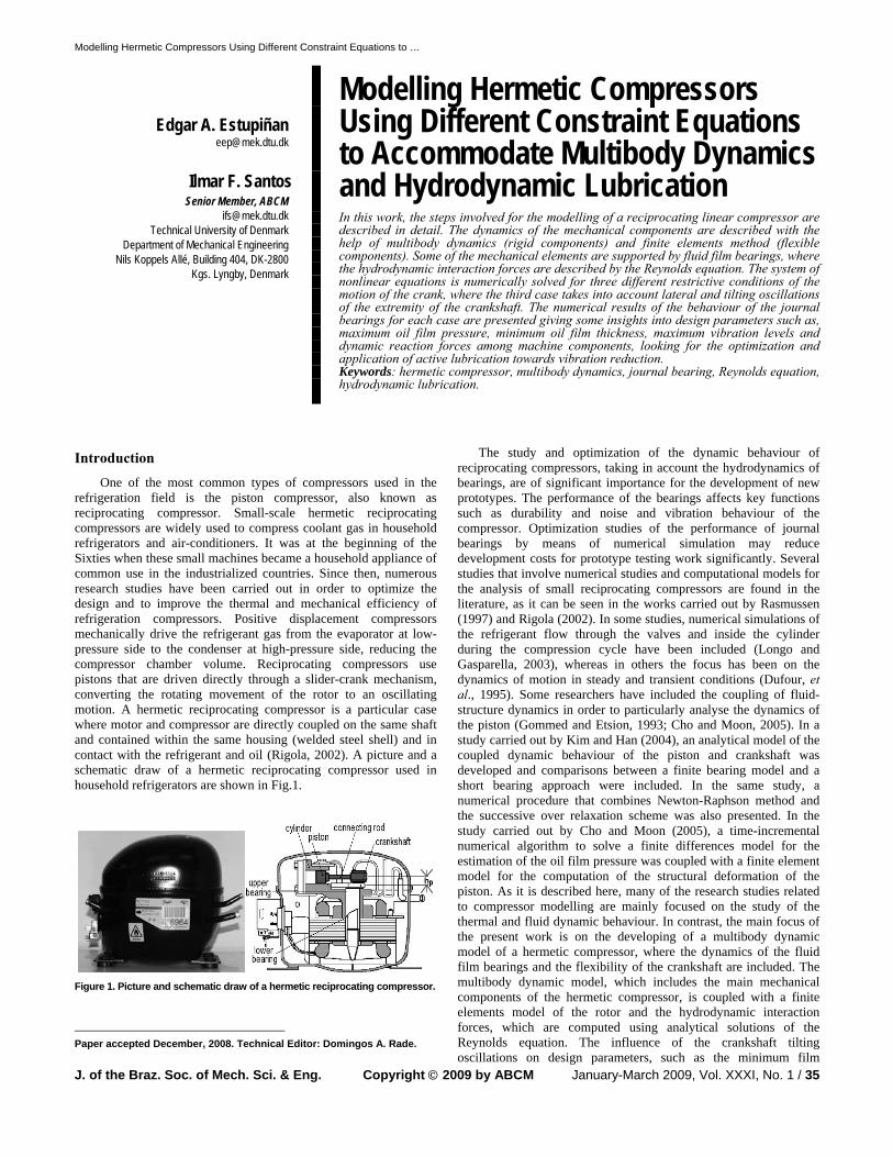
refrigeration field is the piston compressor, also known as reciprocating compressor. Small-scale hermetic reciprocating compressors are widely used to compress coolant gas in household refrigerators and air-conditioners. It was at the beginning of the Sixties when these small machines became a household appliance of common use in the industrialized countries. Since then, numerous research studies have been carried out in order to optimize the design and to improve the thermal and mechanical efficiency of refrigeration compressors. Positive displacement compressors mechanically drive the refrigerant gas from the evaporator at low-pressure side to the condenser at high-pressure side, reducing the compressor chamber volume. Reciprocating compressors use pistons that are driven directly through a slider-crank mechanism, converting the rotating movement of the rotor to an oscillating motion. A hermetic reciprocating compressor is a particular case where motor and compressor are directly coupled on the same shaft and contained within the same housing (welded steel shell) and in contact with the refrigerant and oil (Rigola, 2002). A picture and a schematic draw of a hermetic reciprocating compressor used in household refrigerators are shown in Fig.1.
Figure 1. Picture and schematic draw of a hermetic reciprocating compressor.
Paper accepted December, 2008. Technical Editor: Domingos A. Rade.
The study and optimization of the dynamic behaviour of
reciprocating compressors, taking in account the hydrodynamics of bearings, are of significant importance for the development of new prototypes. The performance of the bearings affects key functions such as durability and noise and vibration behaviour of the compressor. Optimization studies of the performance of journal bearings by means of numerical simulation may reduce development costs for prototype testing work significantly. Several studies that involve numerical studies and computational models for the analysis of small reciprocating compressors are found in the literature, as it can be seen in the works carried out by Rasmussen (1997) and Rigola (2002). In some studies, numerical simulations of the refrigerant flow through the valves and inside the cylinder during the compression cycle have been included (Longo and Gasparella, 2003), whereas in others the focus has been on the dynamics of motion in steady and transient conditions (Dufour, et al., 1995). Some researchers have included the coupling of fluid-structure dynamics in order to particularly analyse the dynamics of the piston (Gommed and Etsion, 1993; Cho and Moon, 2005). In a study carried out by Kim and Han (2004), an analytical model of the coupled dynamic behaviour of the piston and crankshaft was developed and comparisons between a finite bearing model and a short bearing approach were included. In the same study, a numerical procedure that combines Newton-Raphson method and the successive over relaxation scheme was also presented. In the study carried out by Cho and Moon (2005), a time-incremental numerical algorithm to solve a finite differences model for the estimation of the oil film pressure was coupled with a finite element model for the computation of the structural deformation of the piston. As it is described here, many of the research studies related to compressor modelling are mainly focused on the study of the thermal and fluid dynamic behaviour. In contrast, the main focus of the present work is on the developing of a multibody dynamic model of a hermetic compressor, where the dynamics of the fluid film bearings and the flexibility of the crankshaft are included. The multibody dynamic model, which includes the main mechanical components of the hermetic compressor, is coupled with a finite elements model of the rotor and the hydrodynamic interaction forces, which are computed using analytical solutions of the Reynolds equation. The influence of the crankshaft tilting oscillations on design parameters, such as the minimum film

Edgar A. Estupiñan and Ilmar F. Santos
36 / Vol. XXXI, No. 1, January-March 2009 ABCM
thickness and maximum pressures are carefully investigated, since the finite element model allows capturing of such movements. The elasto-hydrodynamic theory, which takes in account the bearing and housing flexibility, is not considered in this work, since it is presented only in very special cases.
Nomenclature
Ap =transversal area of the piston, m2 cb =radial clearance of the bearing, m Dp =piston diameter, m ec =mass eccentricity of the crank, m f =vector of forces, N fb =vector of journal bearing forces, N hb =oil film thickness, m hp =length of crank pin, m I =moment of inertia tensor l =length of the connecting rod, m lb =width of the bearing, m m =mass, kg ndof =number of degrees of freedom Pg =gas pressure inside the cylinder, Pa p =fluid film pressure, Pa rpm =revolutions per minute r =radius, m S =Sommerfeld number Ti =transformation matrix in the coordinate i xB =piston position along the X direction, m Greek Symbols Ω =rotational speed of the crankshaft, rad/s θ =rotation angle of the crank around Z-Z axis, rad α =rotation angle of the connecting rod, rad β =rotation angle around X-X axis, rad Γ =rotation angle around Y1-Y1 axis, rad µ =viscosity oil film, Pa.s ε =eccentricity ratio φ =attitude angle, rad τz =motor shaft torque, Nm Subscripts A,B,C =relative to the points A, B or C, respectively b =relative to the bearing Bi =relative to the i-th mobile reference frame c =relative to the crank cr =relative to the connecting rod p =relative to the piston I =relative to the inertial reference frame N =relative to normal reaction forces cylinder-piston LJB =relative to infinitely long-width journal bearing SJB =relative to short-width journal bearing X,Y =relative to the X and Y directions ξ, η =relative to the radial and transversal directions
Mathematical Modelling
In this section the formulation of representative motion equations to describe the mathematical model of a hermetic reciprocating compressor is developed. The main components of the reciprocating mechanism (i.e., connecting rod and crank) are modelled as rigid bodies, the piston motion is modelled as a particle and the main shaft is modelled as a flexible body via finite elements.
Three different approaches which differ in the definition of the restrictive conditions of motion of the centre of the crank have been comparatively studied. These three cases are:
- Case (I). Neglecting lateral displacements and tilting oscillations of the crank (no hydrodynamic bearings).
- Case (II). Considering lateral displacements but not tilting oscillations of the crank (rigid crankshaft).
- Case (III). Considering lateral displacements and tilting oscillations of the crank (flexible crankshaft).
Although the two first approaches make the problem simpler
and reduce the computational time, by including the tilting crank effect in the model (case III), a more precise estimation of the journal bearing forces and the journal orbits may be obtained, considering that the oil film thickness is usually only a few micrometers thick. In order to include the tilting oscillations of the crank, the crankshaft is modelled via finite elements and coupled to the motion equations of the piston-slider-crank mechanism through the degrees of freedom where the shaft is connected to the crank. Furthermore, the fluid film forces in the upper and lower bearings are calculated by using analytical solutions of the Reynolds equation, and introduced into the equations of the rotor at each time. Therefore, depending on the case of study, the dynamics of the compressor is described by a different global system of equations.
Developing of the Multibody Dynamics Model
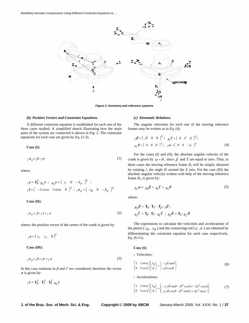
The motion equations of the piston-connecting rod-crank system have been formulated using the Newton-Euler's method, following the methodology suggested by Santos (2001). Figure 2 shows a sketch indicating the inertial referential frame IXYZ and the main angles of rotation for the four moving reference frames.
(a) Definition of the Inertial and Moving Reference Systems.
One inertial reference frame IXYZ and four moving reference frames have been defined. The inertial reference frame is attached to the centre of the bearing (point O), whereas, the moving reference frames B1, B2 and B3 are attached to the crank, and the moving reference frame B4 is attached to the connecting rod. B1 (X1Y1Z1) is obtained by rotating I, the angle β, around the X axis; B2 (X2Y2Z2) is obtained by rotating B1, the angle Γ, around the Y1 axis; B3 (X3Y3Z3) is obtained by rotating B2, the angle θ, around the Z2 axis, and B4 (X4Y4Z4) is obtained by rotating I, the angle α, around the Z axis. The transformation matrices are given by: Tβ: transformation from the inertial frame I to the moving frame B1.
⎥⎥⎥
⎦
⎤
⎢⎢⎢
⎣
⎡
−=
βββββ
cossinsincos
00
001T
TΓ: transformation from the inertial frame B1 to the moving frame B2.
⎥⎥⎥
⎦
⎤
⎢⎢⎢
⎣
⎡ −=
ΓΓ
ΓΓ
Γcossin
sincos
0010
0T
Tθ: transformation from the inertial frame B2 to the moving frame B3.
⎥⎥⎥
⎦
⎤
⎢⎢⎢
⎣
⎡−=
10000
θθθθ
θ cossinsincos
T
Tα: transformation from the inertial frame I to the moving frame B4.
⎥⎥⎥
⎦
⎤
⎢⎢⎢
⎣
⎡ −=
10000
αααα
α cossinsincos
T
Modelling Hermetic Compressors Using Different Constraint Equations to …
J. of the Braz. Soc. of Mech. Sci. & Eng. Copyright © 2009 by ABCM January-March 2009, Vol. XXXI, No. 1 / 37
Figure 2. Geometry and reference systems.
(b) Position Vectors and Constraint Equations.
A different constraint equation is established for each one of the three cases studied. A simplified sketch illustrating how the main parts of the system are connected is shown in Fig. 2. The constraint equations for each case are given by Eq. (1-3).
Case (I):
rlx IIpI =+ (1)
where,
rTr 3BT
I ⋅= θ ; TpcB hr −= 03 r ;
T0αα sinlcoslI −=l ; TpBpI hx −= 0x
Case (II):
crlx IIIpI +=+ (2)
where, the position vector of the centre of the crank is given by:
TccI yx 0=c
Case (III):
crlx IIIpI +=+ (3)
In this case rotations in β and Γ are considered, therefore the vector Ir is given by:
rTTTr 3BTTT
I ⋅⋅⋅= θΓβ
(c) Kinematic Relations.
The angular velocities for each one of the moving reference frames may be written as in Eq. (4).
T00β&& =βI ; T001 Γ&& =ΓB ;
Tθ&& 002 =θB ; Tα&& −= 00αI (4) For the cases (I) and (II), the absolute angular velocity of the
crank is given by θω &= , since β& and Γ& are equal to zero. Thus, in these cases the moving reference frame B3 will be simply obtained by rotating I, the angle θ, around the Z axis. For the case (III) the absolute angular velocity written with help of the moving reference frame B3, is given by:
θβ ω &&&
3333 BBBB ++= Γ (5)
where:
ββ &&
IB ⋅⋅⋅= βΓθ TTT3 ;
ΓΓ &&13 BB ⋅⋅= Γθ TT ; θθ &&
23 BB ⋅= θT
The expressions to calculate the velocities and accelerations of
the piston ( Bx& , Bx&& ) and the connecting rod (α& ,α&& ) are obtained by differentiating the constraint equation for each case respectively, Eq. (6-11).
Case (I):
- Velocities:
⎭⎬⎫
⎩⎨⎧−
=⎭⎬⎫
⎩⎨⎧
⎥⎦
⎤⎢⎣
⎡θθθθ
ααα
cosrsinrx
coslsinl
c
cB&
&
&
&
01 (6)
- Accelerations:
⎪⎭
⎪⎬⎫
⎪⎩
⎪⎨⎧
+−−−−=
⎭⎬⎫
⎩⎨⎧
⎥⎦
⎤⎢⎣
⎡
ααθθθθααθθθθ
ααα
sinl)sincos(rcosl)cossin(rx
coslsinl
c
cB22
22
01
&&&&
&&&&
&&
&& (7)
Edgar A. Estupiñan and Ilmar F. Santos
38 / Vol. XXXI, No. 1, January-March 2009 ABCM
Case (II):
- Velocities:
⎭⎬⎫
⎩⎨⎧
++−
=⎭⎬⎫
⎩⎨⎧
⎥⎦
⎤⎢⎣
⎡
Cc
CcB
ycosrxsinrx
coslsinl
&&
&&
&
&
θθθθ
ααα
01 (8)
- Accelerations:
⎪⎭
⎪⎬⎫
⎪⎩
⎪⎨⎧
++−+−−−=
⎭⎬⎫
⎩⎨⎧
⎥⎦
⎤⎢⎣
⎡
Cc
CcB
ysinl)sincos(rxcosl)cossin(rx
coslsinl
&&&&&&
&&&&&&
&&
&&
ααθθθθααθθθθ
ααα
22
22
01 (9)
Case (III):
- Velocities
⎭⎬⎫
⎩⎨⎧
=⎭⎬⎫
⎩⎨⎧
⎥⎦
⎤⎢⎣
⎡
2
101
wwx
coslsinl B
ααα
&
& (10)
- Accelerations:
⎭⎬⎫
⎩⎨⎧
=⎭⎬⎫
⎩⎨⎧
⎥⎦
⎤⎢⎣
⎡
4
301
wwx
coslsinl B
ααα
&&
&& (11)
where:
Cpc xch)sccs(rw &&&& +−+−= ΓΓθΓθθΓΓ1 (12)
Cppc
cc
ycch)sshccsr(
)ssscc(r)sscsc(rw&&&
&&
++−+
−+−=
ΓββΓβθΓβΓ
θΓβθβθθβθΓββ2 (13)
Ccp
cccpc
xclscrch
ccrssr)ccrsh(csrw
&&&&&&&
&&&&&&
+−−−
−+−+−=
ααθΓθΓΓ
θΓθθΓΓθθΓΓΓθΓΓ2
22
3 2 (14)
Cc
cpc
cpc
ccppc
pccc
ysl)ssscc(r
scsr)schcccr(
)ssccs(r)sshccsr(
)cscrssrcch()cshcssr(
)cshcssrscr()csssc(rw
&&&&&
&&&&
&&&&
&&&
&&
++−+
−−+
+−−+
+−++−
++−+−=
ααθΓβθβθ
θΓβΓθΓβθΓβΓβ
θΓβθββθΓβθΓβΓ
θΓβθβΓββΓβθΓβΓ
ΓβθΓβθββθΓβθβθ
2
2
224
22
2 (15)
In Eq.(12-15):
θθ sins = ; θθ cosc = ; αα sins = ; αα cosc = ; ββ sins = ; ββ cosc = ; ΓΓ sins = ; ΓΓ cosc = .
(d) Equations of Motion.
The equations of motion for each body and for the case (III) are given by Eq. (16-20). Since the piston is not the focus of the present analysis, it should be noticed that in the modelling of the piston the friction forces are not included.
Crank
T cccAIcIcI y,xmm &&&&=⇒⋅=∑ faf (16)
( ) ( )CBcmCBc
BcBBBcBBABBCB
mdtd
ar
ωIωωIτfrM
33
333333333
×⋅+
⋅×+⋅=+×=
−
∑ (17)
where,
AIAB fTTTf ⋅⋅⋅= βΓθ3; T zB ,, τ003 =τ ; T 003 ,,eccmCB =−r
Connecting Rod
BIAIcrIcrI m ffaf +=⋅=∑ (18)
( ) ( )BBcrBcr
BcrBBBcrBABBBB
mdtd
ar
αIααIflM
44
44444444
×⋅+
⋅×+⋅=×=∑ &&& (19)
where,
( )( )
⎪⎪⎭
⎪⎪⎬
⎫
⎪⎪⎩
⎪⎪⎨
⎧
−++
=
×+××+=
0
2
2
αααααααα
sincosrsincosrx
cr
crB
crIIcrIIIBIcrI
&&&
&&&&&
&&&&
rαrααaa
;
AIAB fTf ⋅= α4; BIBB aTa ⋅= α4
; T 00 ,,BxBI &&=a
Piston
pINIBIBIpBI m fffaf ++=⋅=∑ (20)
where,
T 00 ,,AP pgpI ⋅=f For each case the equations of motion may be written in a matrix
form as in Eq. (21), where the vector b contains the main unknowns (i.e., reaction forces, reaction moments and accelerations). This matrix system is fully described for each case in the appendices A, B and C respectively. For the case (III), where the flexibility of the shaft is included, the matrix system of Eq. (21) has to be coupled to the motion equations of the rotor obtained via a finite elements formulation, which is presented in the next sections.
cbA =⋅ (21)
Modelling of the Rotor
For the case (III), the main shaft of the compressor is considered as a simply rotating beam, supported by the upper and lower bearings, as illustrated in Fig. 1. The shaft is modelled as a flexible body using a finite elements formulation for a rotor bearing system, which includes gyroscopic and rotatory inertia effects (Nelson and McVaugh, 1976). Considering that the main focus of this study is on the lower mode shapes, the use of this formulation is appropriated to this case and only few finite elements have been used to model the rotor. The global equation of motion can be written as in Eq. (22), where, M , K , G are the mass, stiffness and gyroscopic matrices respectively, and f is the vector of loads on the rotor, which includes: static preload forces (
plI f ), unbalance rotor
forces ( ubI f ) and the hydrodynamic bearing forces ( bI f ). Based on the fluid film theory, the bearing forces are calculated by using analytical solutions of the Reynolds equation. These forces depend on the linear displacements and velocities of the nodes that in the finite element model represent the journal bearings centre.
Modelling Hermetic Compressors Using Different Constraint Equations to …
J. of the Braz. Soc. of Mech. Sci. & Eng. Copyright © 2009 by ABCM January-March 2009, Vol. XXXI, No. 1 / 39
44 344 21&&&
f
qKqGfqMˆ
⋅−⋅−=⋅ (22)
Fluid Film Forces
The governing equation for the pressure distribution of the oil film in dynamically loaded journal bearings is given by Eq. (23). This equation is obtained from the general formulation of the Reynolds equation (Hamrock, 1991). In this equation, φ& is the rotational speed of the journal centre about the bearing centre and ε is the relative eccentricity.
⎥⎦
⎤⎢⎣
⎡⎟⎠⎞
⎜⎝⎛ −
∂∂
+∂∂
=⎟⎟⎠
⎞⎜⎜⎝
⎛
∂∂
∂∂
+⎟⎟⎠
⎞⎜⎜⎝
⎛
∂∂
∂∂
212 2
32
3 Ωφϕεϕ
εµϕµϕ t
sincost
rczph
zrph
bbb
bb (23)
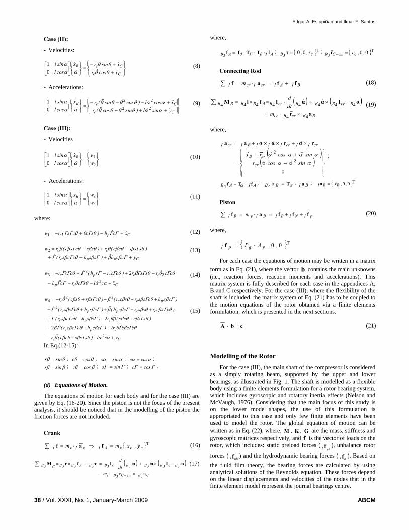
The main geometric parameters and reference frames used to
describe a journal bearing are shown in Fig. 3. The fluid film thickness around the bearing circumference can be calculated by using the expression: )cos(ch bb ϕε+= 1 , where ϕ is the angle measured from the location of the maximum film thickness. In dynamically loaded bearings, the eccentricity and attitude angle will vary through the loading cycle. Therefore, the fluid film pressure distribution at any eccentricity ratio may be determined only if the normal squeeze velocity (ε& ) and the rotational velocities ( Ω ,φ& ) are known for the same eccentricity ratio. Complete solutions of Eq. (23) may be obtained numerically, and solutions for limited cases may be also obtained analytically.
Figure 3. Journal bearing geometry.
In this work, analytical solutions for the short-width bearing
(SJB) and infinitely-long-width bearing (LJB) theories have been used. The short-journal-bearing theory assumes that the variation of pressure is more significant in the axial direction than in the circumferential direction, and therefore the first term on the left side of Eq. (23) can be neglected. In contrast, for an infinitely long-width-journal-bearing, the pressure in the axial direction is assumed to be constant, and therefore the side-leakage term, i.e., the second term on the left side of Eq. (23) can be neglected. Thus, the modified Reynolds equation for each case can be integrated twice and analytical expressions for the pressure distribution can be found. Assuming that the bearing is well aligned and the viscosity of the lubricant keeps constant, the pressure distribution for a SJB and a LJB is given by Eq. (24-25).
⎥⎦
⎤⎢⎣
⎡∂∂
+∂∂
⎟⎠
⎞⎜⎝
⎛∂∂
−⎟⎟⎠
⎞⎜⎜⎝
⎛−−=
tcosc
ht
zl
hp b
bb
bSJB
εϕϕ
φΩµ 224
3 22
3 (24)
( )( )( )
( ) ( ) ⎪⎭
⎪⎬⎫
⎥⎥⎦
⎤
⎢⎢⎣
⎡
+−
+∂∂
+
⎪⎩
⎪⎨⎧
++
+⎟⎠⎞
⎜⎝⎛
∂∂
−⎟⎟⎠
⎞⎜⎜⎝
⎛=
22
22
2
11
111
12226
εϕε
εε
ϕεε
ϕεϕεφΩµ
cost
coscossin
tcrpb
bLJB (25)
The journal bearing forces are calculated by integrating the
pressure distribution. If the pressure is integrated over all the fluid film around the bearing (i.e, πϕ 20 ≤≤ ), the analytical solution is known as a full Sommerfeld solution. However, if the analysis is limited to the convergent film (i.e., πϕ ≤≤0 ), the analytical solution is known as a half Sommerfeld solution. Because in real bearings pressures lower than the ambient’s are rarely found, and using the last approach more realistic predictions may be obtained (Hamrock, 1991). Thus, the analytical expressions to calculate the bearing forces in ξ , η coordinates, using the half Sommerfeld conditions for the SJB and LJB approaches respectively, are given by Eq. (26-29). A detailed procedure to obtain these expressions is included in the reference (Frêne, 1990).
Hydrodynamic fluid film forces: Short-journal-bearing
⎥⎥⎦
⎤
⎢⎢⎣
⎡⎟⎠⎞
⎜⎝⎛
∂∂
−+∂∂
−
+
−
−=
tt)()(
)(clrF /
b
bb φΩεεε
επε
µξ 22
121
122
212
2
222
3 (26)
⎥⎥⎦
⎤
⎢⎢⎣
⎡⎟⎠⎞
⎜⎝⎛
∂∂
−−
+∂∂
−=
t)(
t)(clrF
/
b
bb φΩ
επεεεµ
η 22
1412
212
222
3 (27)
Hydrodynamic fluid film forces: Infinitely-long-journal-bearing
⎥⎥⎦
⎤
∂∂
⎟⎟⎠
⎞⎜⎜⎝
⎛
+−⎟
⎟⎠
⎞⎜⎜⎝
⎛
−+
⎢⎢⎣
⎡⎟⎠⎞
⎜⎝⎛
∂∂
−−+
−=
t)()(
t))((clrF
/
b
bb
εεπ
πε
φΩ
εεεµ
ξ
2232
22
2
2
3
28
211
212
12
(28)
⎥⎥⎦
⎤
∂∂
⎟⎟⎠
⎞⎜⎜⎝
⎛
−++
⎢⎢⎣
⎡⎟⎠⎞
⎜⎝⎛
∂∂
−−+
=
t))((
t))((clrF /
b
bb
εεε
ε
φΩ
εεπεµ
η
22
21222
3
122
2122
12
(29)
In order to describe the fluid film forces in the inertial reference
frame, the transformation given by Eq. (30) is used, where the attitude angle )t(φ is the angle measured between the X-axis and the location of the minimum oil film thickness. For the case (II), the bearing forces XF and YF are coupled directly to the vector c of Eq. (21), whereas, for the case (III), they correspond to the components of the vector bI f of Eq. (22).
⎭⎬⎫
⎩⎨⎧
⎥⎦
⎤⎢⎣
⎡ −=
⎭⎬⎫
⎩⎨⎧
η
ξ
φφφφ
FF
)t(cos)t(sin)t(sin)t(cos
FF
Y
X (30)
Numerical Implementation
The equations of motion that describe the dynamics of the system together with the FEM model of the shaft and the analytical expressions for the fluid film forces yield to a system of high complexity and non-linearity. A flowchart, with the main steps
Edgar A. Estupiñan and Ilmar F. Santos
40 / Vol. XXXI, No. 1, January-March 2009 ABCM
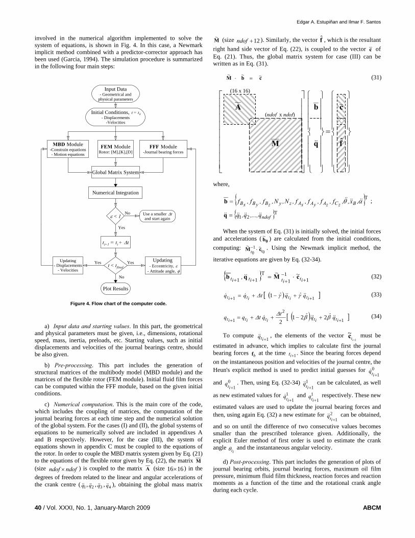
involved in the numerical algorithm implemented to solve the system of equations, is shown in Fig. 4. In this case, a Newmark implicit method combined with a predictor-corrector approach has been used (Garcia, 1994). The simulation procedure is summarized in the following four main steps:
Plot Results
Numerical Integration
No
YesYes
No
Yes
Global Matrix System
Input Data- Geometrical and
physical parameters
ti+1 = ti + ∆t
t < tfinal
Use a smaller ∆tand start againε < 1
Updating - Eccentricity, ε
- Attitude angle, φ
Updating- Displacements
- Velocities
FEM ModuleRotor: [M],[K],[D]
MBD Module-Constrain equations- Motion equations
Initial Conditions, t = t0- Displacements
-Velocities
FFF Module-Journal bearing forces
Figure 4. Flow chart of the computer code.
a) Input data and starting values. In this part, the geometrical
and physical parameters must be given, i.e., dimensions, rotational speed, mass, inertia, preloads, etc. Starting values, such as initial displacements and velocities of the journal bearings centre, should be also given.
b) Pre-processing. This part includes the generation of structural matrices of the multibody model (MBD module) and the matrices of the flexible rotor (FEM module). Initial fluid film forces can be computed within the FFF module, based on the given initial conditions.
c) Numerical computation. This is the main core of the code, which includes the coupling of matrices, the computation of the journal bearing forces at each time step and the numerical solution of the global system. For the cases (I) and (II), the global systems of equations to be numerically solved are included in appendixes A and B respectively. However, for the case (III), the system of equations shown in appendix C must be coupled to the equations of the rotor. In order to couple the MBD matrix system given by Eq. (21) to the equations of the flexible rotor given by Eq. (22), the matrix M (size ndofndof × ) is coupled to the matrix A (size 1616× ) in the degrees of freedom related to the linear and angular accelerations of the crank centre ( 1q&& , 2q&& , 3q&& , 4q&& ), obtaining the global mass matrix
M~ (size 12+ndof ). Similarly, the vector f , which is the resultant right hand side vector of Eq. (22), is coupled to the vector c of Eq. (21). Thus, the global matrix system for case (III) can be written as in Eq. (31).
cbM ~~~ =⋅ (31)
where,
Tαθ &&&&&& ,x,,f,f,f,f,N,N,f,f,f BzCzAyAxAzyzByBxB=b ;
Tndofq,...,q,q &&&&&&&& 21=q When the system of Eq. (31) is initially solved, the initial forces
and accelerations ( 0b~ ) are calculated from the initial conditions, computing:
01
0 tt~~ cM ⋅− . Using the Newmark implicit method, the
iterative equations are given by Eq. (32-34).
11
111 +−
+++ ⋅= itititit~~, cMqb T
&& (32)
[ ( ) ]11 1 ++ +−+= itititit qˆqˆtqq &&&&&& γγ∆ (33)
[ ( ) ]1
2
1 2212 ++ +−++= ititititit qˆqˆtqtqq &&&&& ββ∆∆ (34)
To compute
1+itq&& , the elements of the vector 1
~+it
c must be
estimated in advance, which implies to calculate first the journal bearing forces bf at the time 1+it . Since the bearing forces depend on the instantaneous position and velocities of the journal centre, the Heun's explicit method is used to predict initial guesses for 0
1+itq&
and 01+it
q . Then, using Eq. (32-34) 11+it
q&& can be calculated, as well
as new estimated values for 11+it
q& and 11+it
q respectively. These new
estimated values are used to update the journal bearing forces and then, using again Eq. (32) a new estimate for 2
1+itq&& can be obtained,
and so on until the difference of two consecutive values becomes smaller than the prescribed tolerance given. Additionally, the explicit Euler method of first order is used to estimate the crank angle
itθ and the instantaneous angular velocity.
d) Post-processing. This part includes the generation of plots of journal bearing orbits, journal bearing forces, maximum oil film pressure, minimum fluid film thickness, reaction forces and reaction moments as a function of the time and the rotational crank angle during each cycle.
(16 x 16)
(ndof x ndof)
⎪⎪⎪⎪
⎭
⎪⎪⎪⎪
⎬
⎫
⎪⎪⎪⎪
⎩
⎪⎪⎪⎪
⎨
⎧
=
⎪⎪⎪⎪
⎭
⎪⎪⎪⎪
⎬
⎫
⎪⎪⎪⎪
⎩
⎪⎪⎪⎪
⎨
⎧
⎥⎥⎥⎥⎥⎥⎥⎥⎥
⎦
⎤
⎢⎢⎢⎢⎢⎢⎢⎢⎢
⎣
⎡
ˆ
f
c
q
b
M
A
&&

Modelling Hermetic Compressors Using Different Constraint Equations to …
J. of the Braz. Soc. of Mech. Sci. & Eng. Copyright © 2009 by ABCM January-March 2009, Vol. XXXI, No. 1 / 41
Results and Discussion
The system of equations described in the previous sections has been numerically solved for each one of the three approaches presented. Particularly, the numerical results have been analysed with focus on the behaviour of the main bearing of the crankshaft (upper journal bearing shown in Fig. 1. The main geometrical dimensions and physical properties of the reciprocating compressor used in this study are given in table 1. The gas pressure as a function of the crank angle is taken from Cho and Moon (2005) and it is shown in Fig. 5a. The variation of torque in function of the angular velocity for a hermetic compressor with similar characteristics to the one used in this work is taken from Rigola (2002) and it is shown in Fig. 5b.
Table 1. Main geometrical and physical parameters.
Radius crank-pin centre rc 7.5 mm Radius of bearings rb 8 mm Width of bearings lb 6 mm Journal clearance cb 15 µm Length crank pin hp 10 mm Distance between bearings L 80 mm Inertia of motor-rotor Ix, Iy = 0.4x10⁻³ ; Iz = 0.1x10⁻² kg.m2 Diameter of piston Dp 23 mm (Ap = 415.5 mm2) Length of the piston lp 22 mm Mass of the piston mp 0.043 kg Lubricant viscosity µ 0.005 Pa.s Angular velocity Ω 312 rad/s (2980 rpm) Mass eccentricity of crank ec 5 mm
(a)
(b)
Figure 5. (a) Curve of the gas pressure (Pg) as a function of the crankshaft angle. (b) Curve of the motor torque ( zτ ) as a function of the angular velocity.
Results - Case (I)
In this case, lateral displacements and tilting oscillations of the crank are neglected. Therefore, the hydrodynamic bearing forces are not calculated, but instead the reaction forces and the reaction moments at the centre of the crank are calculated. The reaction forces in the joint crank pin-connecting rod (fA) and in the joint piston-connecting rod (fB) are shown in Fig. 6. The plot of the reaction moments is shown in Fig. 7. The maximum forces are found close to the top dead centre and it can be seen clearly that the reaction forces in X-direction are dominated by the compression force coming from the piston and the inertial effects.
(a)
(b)
Figure 6. Reaction forces. (a) Joint piston-connecting rod. (b) Joint crank-connecting rod – case(I).
Figure 7. Crank reaction moments – case (I).
Results - Case (II)
In this case, tilting oscillations of the crank are neglected and lateral displacements are allowed. The hydrodynamic journal forces for the upper bearing are computed using Eq. (26-27) and they are shown in Fig. 8. It can be seen from this figure that the upper bearing forces are similar to the reaction forces obtained for case (I), which is expected, due to the fact that the equilibrium conditions have to be always accomplished, even if the crank centre is allowed to have lateral oscillations.
Edgar A. Estupiñan and Ilmar F. Santos
42 / Vol. XXXI, No. 1, January-March 2009 ABCM
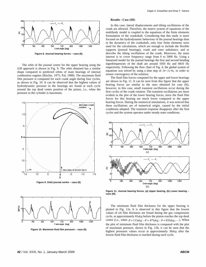
Figure 8. Journal bearing forces – case (II).
The orbit of the journal centre for the upper bearing using the
SJB approach is shown in Fig. 9. The orbit obtained has a similar shape compared to predicted orbits of main bearings of internal combustion engines (Ritchie, 1975; Pal, 1988). The maximum fluid film pressure is computed for each crank angle during four cycles, as shown in Fig. 10. It can be observed that the highest values of hydrodynamic pressure in the bearings are found at each cycle around the top dead centre position of the piston, i.e., when the pressure in the cylinder is maximum.
Figure 9. Orbit journal centre – case (II).
Figure 10. Maximum fluid film pressure – case (II).
Results - Case (III)
In this case, lateral displacements and tilting oscillations of the crank are allowed. Therefore, the matrix system of equations of the multibody model is coupled to the equations of the finite elements formulation of the crankshaft. Considering that this study is more focused on the hydrodynamic behaviour of the journal bearings than in the dynamics of the crankshaft, only four finite elements were used for the calculations, which are enough to include the flexible supports (journal bearings), crank and rotor unbalance, and to describe the tilting oscillations of the crank. Moreover, the main interest is to cover frequency range from 0 to 5000 Hz. Using a linearized model for the journal bearings the first and second bending eigenfrequencies of the shaft are around 1050 Hz and 6810 Hz respectively. Following the flow chart of Fig. 4, the global system of equations was solved by using a time step of ∆t=1e-6s, in order to ensure convergence of the solution.
The fluid film forces computed for the upper and lower bearings are shown in Fig. 11. It can be seen from this figure that the upper bearing forces are similar to the ones obtained for case (II), however, in this case, small transient oscillations occur during the first cycles of the crank rotation. The transient oscillations are more evident in the plot of the lower bearing forces, since the fluid film forces for this bearing are much lower compared to the upper bearing forces. During the numerical simulations, it was noticed that these oscillations are of numerical origin, caused by the initial conditions adopted. The transient response disappears after the first cycles and the system operates under steady-state conditions.
(a)
(b)
Figure 11. Journal bearing forces. (a) Upper bearing, (b) Lower bearing – case (III).
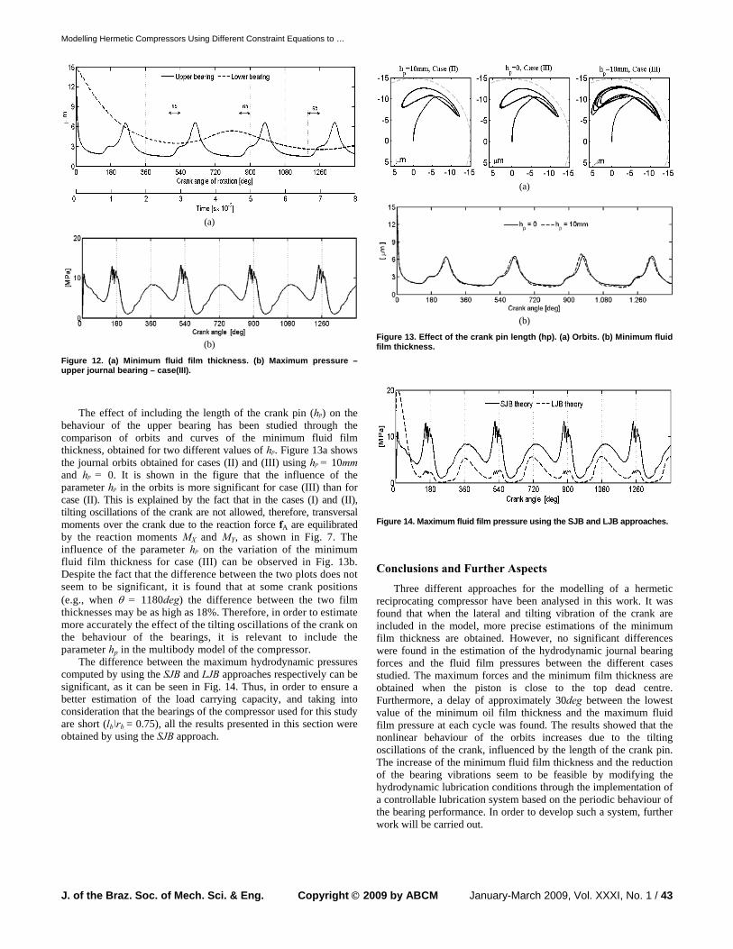
The minimum fluid film thickness for the upper bearing is
plotted in Fig. 12a. It is observed in this figure that the lowest values of oil film thickness are found during the gas compression cycle, at approximately 65deg before the piston reaches the top dead centre (i.e., when deg115≈θ , deg475≈θ , deg835≈θ ,…). When the plot of minimum fluid film thickness is compared with the plot of maximum pressure, shown in Fig. 12b, it can be seen that the highest pressures values occur at approximately 30deg after the lowest fluid film thickness is reached during each cycle.
Modelling Hermetic Compressors Using Different Constraint Equations to …
J. of the Braz. Soc. of Mech. Sci. & Eng. Copyright © 2009 by ABCM January-March 2009, Vol. XXXI, No. 1 / 43
(a)
(b)
Figure 12. (a) Minimum fluid film thickness. (b) Maximum pressure – upper journal bearing – case(III).
The effect of including the length of the crank pin (hp) on the
behaviour of the upper bearing has been studied through the comparison of orbits and curves of the minimum fluid film thickness, obtained for two different values of hp. Figure 13a shows the journal orbits obtained for cases (II) and (III) using hp = 10mm and hp = 0. It is shown in the figure that the influence of the parameter hp in the orbits is more significant for case (III) than for case (II). This is explained by the fact that in the cases (I) and (II), tilting oscillations of the crank are not allowed, therefore, transversal moments over the crank due to the reaction force fA are equilibrated by the reaction moments MX and MY, as shown in Fig. 7. The influence of the parameter hp on the variation of the minimum fluid film thickness for case (III) can be observed in Fig. 13b. Despite the fact that the difference between the two plots does not seem to be significant, it is found that at some crank positions (e.g., when θ = 1180deg) the difference between the two film thicknesses may be as high as 18%. Therefore, in order to estimate more accurately the effect of the tilting oscillations of the crank on the behaviour of the bearings, it is relevant to include the parameter hp in the multibody model of the compressor.
The difference between the maximum hydrodynamic pressures computed by using the SJB and LJB approaches respectively can be significant, as it can be seen in Fig. 14. Thus, in order to ensure a better estimation of the load carrying capacity, and taking into consideration that the bearings of the compressor used for this study are short (lb\rb = 0.75), all the results presented in this section were obtained by using the SJB approach.
(a)
(b)
Figure 13. Effect of the crank pin length (hp). (a) Orbits. (b) Minimum fluid film thickness.
Figure 14. Maximum fluid film pressure using the SJB and LJB approaches.
Conclusions and Further Aspects
Three different approaches for the modelling of a hermetic reciprocating compressor have been analysed in this work. It was found that when the lateral and tilting vibration of the crank are included in the model, more precise estimations of the minimum film thickness are obtained. However, no significant differences were found in the estimation of the hydrodynamic journal bearing forces and the fluid film pressures between the different cases studied. The maximum forces and the minimum film thickness are obtained when the piston is close to the top dead centre. Furthermore, a delay of approximately 30deg between the lowest value of the minimum oil film thickness and the maximum fluid film pressure at each cycle was found. The results showed that the nonlinear behaviour of the orbits increases due to the tilting oscillations of the crank, influenced by the length of the crank pin. The increase of the minimum fluid film thickness and the reduction of the bearing vibrations seem to be feasible by modifying the hydrodynamic lubrication conditions through the implementation of a controllable lubrication system based on the periodic behaviour of the bearing performance. In order to develop such a system, further work will be carried out.
Edgar A. Estupiñan and Ilmar F. Santos
44 / Vol. XXXI, No. 1, January-March 2009 ABCM
Acknowledgments
The authors gratefully acknowledge the support given by the Programme Alβan, the European Union Programme of High Level Scholarships for Latin America, scholarship No. E06D101992CO.
References Cho, J. R. and Moon, S.J., 2005, “A Numerical Analysis of the
Interaction between the Piston Oil Film and the Component Deformation in a Reciprocating Compressor”, Tribology International, Vol.38, pp. 459-468.
Dufour, R., Der Hagopian, J. and Lalanne, M., 1995, “Transient and Steady State Dynamic Behaviour of Single Cylinder Compressors: Prediction and Experiments”, Journal of Sound and Vibration, Vol.181, pp. 23-41.
Frêne, J., Nicolas, D., Degueurce, B., Berthe, D. and Godet, M., 1990, “Lubrification Hydrodynamique”, Ed. Eyrolles, Paris, 488 p.
Garcia de Jalon, J. and Bayo, E., 1994, “Kinematic and Dynamic Simulation of Multibody Systems”, Ed. Springer-Verlag, New-York, 440 p.
Gommed, K. and Etsion, I., 1993, “Dynamic Analysis of Gas Lubricated Reciprocating Ringless Pistons - Basic Modelling”, Journal of Tribology, Vol.115, pp. 207-213.
Hamrock, B. J., 1991, “Fundamental of Fluid Film Lubrication”, NASA Reference Publication, USA, 635 p.
Kim, T. J. and Han, J. S., 2004, “Comparison of the Dynamic Behavior and Lubrication Characteristics of a Reciprocating Compressor Crankshaft in Both Finite and Short Bearing Models”, Tribology Transactions, Vol.47, No.1, pp. 61-69.
Longo, G. and Gasparella, A. 2003, “Unsteady State Analysis of the Compression Cycle of a Hermetic Reciprocating Compressor”, International Journal of Refrigeration, Vol.26, pp. 681-689.
Nelson, H. D. and McVaugh, J. M., 1976, “The dynamics of Rotor-Bearing Systems Using Finite Elements”, Journal of Engineering for Industry, Vol.98, pp. 593-600.
Pal, R., Sinhasan, R. and Singh, D.V, 1988, “Analysis of a Big-End Bearing - a Finite Element Approach”, Wear, Vol.121, No.1, pp. 117-120.
Rasmussen, B.D., 1997, “Variable Speed Hermetic Reciprocating Compressors for Domestic Refrigerators”, Ph.D. Thesis, Technical University of Denmark, Lyngby, Denmark, Vol.1, 158 p.
Rigola, S. J., 2002, “Numerical Simulation and Experimental Validation of Hermetic Reciprocating Compressors”, Ph.D. Thesis, Universidad Politécnica de Cataluña, Barcelona, Spain, 109 p.
Ritchie, G.S., 1975, “The Prediction of Journal Loci in Dynamically Loaded Internal Combustion Engine Bearings”, Wear, Vol.35, No.2, pp. 291-297.
Santos, I. F., 2001, “Dinâmica de Sistemas Mecanicos”, Ed. Makron Books, Sao Paulo, Brasil, 272 p.
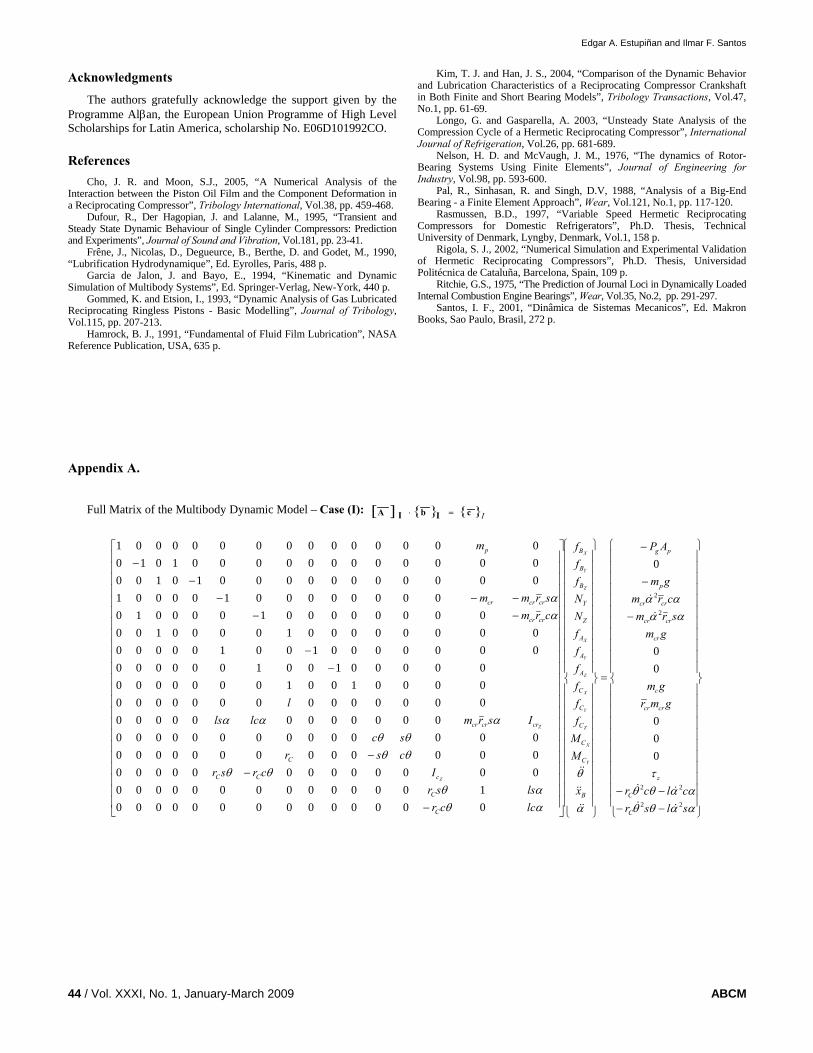
Appendix A.
Full Matrix of the Multibody Dynamic Model – Case (I): [ ] IcIbI A =⋅
⎪⎪⎪⎪⎪⎪⎪⎪⎪⎪⎪
⎭
⎪⎪⎪⎪⎪⎪⎪⎪⎪⎪⎪
⎬
⎫
⎪⎪⎪⎪⎪⎪⎪⎪⎪⎪⎪
⎩
⎪⎪⎪⎪⎪⎪⎪⎪⎪⎪⎪
⎨
⎧
−−−−
−
−
−
=
⎪⎪⎪⎪⎪⎪⎪⎪⎪⎪⎪
⎭
⎪⎪⎪⎪⎪⎪⎪⎪⎪⎪⎪
⎬
⎫
⎪⎪⎪⎪⎪⎪⎪⎪⎪⎪⎪
⎩
⎪⎪⎪⎪⎪⎪⎪⎪⎪⎪⎪
⎨
⎧
⎥⎥⎥⎥⎥⎥⎥⎥⎥⎥⎥⎥⎥⎥⎥⎥⎥⎥⎥⎥⎥⎥⎥
⎦
⎤
⎢⎢⎢⎢⎢⎢⎢⎢⎢⎢⎢⎢⎢⎢⎢⎢⎢⎢⎢⎢⎢⎢⎢
⎣
⎡
−
−−
−−
−−−−−
−−
ααθθααθθ
τ
αααα
α
θ
αθαθ
θθθθθθ
ααα
αα
slsrclcr
gmrgm
gmsrm
crmgm
AP
x
MMffffffNNfff
lccrlssr
Icrsrcsrsc
Isrmlclsl
crmsrmm
m
C
C
z
crcr
c
cr
crcr
crcr
p
pg
B
C
C
C
C
C
A
A
A
Z
Y
B
B
B
C
C
cCC
C
crcrcr
crcr
crcrcr
p
Y
X
Z
Y
X
Z
Y
X
Z
Y
X
Z
Z
22
22
2
2
000
00
0
0000000000000010000000000000
0000000000000000000000000000000000000000
00000000000000000000000000000010010000000000001001000000
00000001001000000000000010000100
00000000100001000000000100001
00000000000101000000000000001010000000000000001
&&
&&
&
&
&&
&&
&&
Modelling Hermetic Compressors Using Different Constraint Equations to …
J. of the Braz. Soc. of Mech. Sci. & Eng. Copyright © 2009 by ABCM January-March 2009, Vol. XXXI, No. 1 / 45
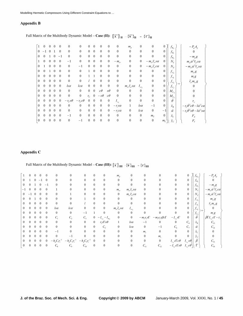
Appendix B
Full Matrix of the Multibody Dynamic Model – Case (II): [ ] IIcIIbII A =⋅
⎪⎪⎪⎪⎪⎪⎪⎪⎪⎪⎪
⎭
⎪⎪⎪⎪⎪⎪⎪⎪⎪⎪⎪
⎬
⎫
⎪⎪⎪⎪⎪⎪⎪⎪⎪⎪⎪
⎩
⎪⎪⎪⎪⎪⎪⎪⎪⎪⎪⎪
⎨
⎧
−−−−
−
−
−
=
⎪⎪⎪⎪⎪⎪⎪⎪⎪⎪⎪
⎭
⎪⎪⎪⎪⎪⎪⎪⎪⎪⎪⎪
⎬
⎫
⎪⎪⎪⎪⎪⎪⎪⎪⎪⎪⎪
⎩
⎪⎪⎪⎪⎪⎪⎪⎪⎪⎪⎪
⎨
⎧
⎥⎥⎥⎥⎥⎥⎥⎥⎥⎥⎥⎥⎥⎥⎥⎥⎥⎥⎥⎥⎥⎥⎥
⎦
⎤
⎢⎢⎢⎢⎢⎢⎢⎢⎢⎢⎢⎢⎢⎢⎢⎢⎢⎢⎢⎢⎢⎢⎢
⎣
⎡
−−
−−−−
−−−
−−−−−
−−
Y
X
C
C
z
crcr
c
cr
crcr
crcr
p
pg
C
C
B
C
C
C
A
A
A
Z
Y
B
B
B
C
C
c
c
cCC
C
crcrcr
crcr
crcrcr
p
FF
slsrclcr
gmrgmgm
srmcrm
gm
AP
yx
x
MMffffNNfff
mm
lccrlssr
Icrsrcsrsc
Isrmlclsl
crmsrmm
m
Y
X
Z
Z
Y
X
Z
Y
X
Z
Z
ααθθααθθ
τ
αααα
α
θ
αααα
θθθθθθ
ααα
αα
22
22
2
2
000
0
00000000100000000000000010000010000000000000
011000000000000000000000000000000000000000000000000000000000000000000000000000000000000011000000000000000100001000000000010000100000000010000100000000000101000000000000001010000000000000001
&&
&&
&
&
&&
&&
&&
&&
&&
Appendix C
Full Matrix of the Multibody Dynamic Model – Case (III): [ ] IIIcIIIbIII A =⋅
⎪⎪⎪⎪⎪⎪⎪⎪⎪⎪⎪
⎭
⎪⎪⎪⎪⎪⎪⎪⎪⎪⎪⎪
⎬
⎫
⎪⎪⎪⎪⎪⎪⎪⎪⎪⎪⎪
⎩
⎪⎪⎪⎪⎪⎪⎪⎪⎪⎪⎪
⎨
⎧
−ΓΓ
−−
−
−
=
⎪⎪⎪⎪⎪⎪⎪⎪⎪⎪⎪
⎭
⎪⎪⎪⎪⎪⎪⎪⎪⎪⎪⎪
⎬
⎫
⎪⎪⎪⎪⎪⎪⎪⎪⎪⎪⎪
⎩
⎪⎪⎪⎪⎪⎪⎪⎪⎪⎪⎪
⎨
⎧
Γ⎥⎥⎥⎥⎥⎥⎥⎥⎥⎥⎥⎥⎥⎥⎥⎥⎥⎥⎥⎥⎥⎥⎥
⎦
⎤
⎢⎢⎢⎢⎢⎢⎢⎢⎢⎢⎢⎢⎢⎢⎢⎢⎢⎢⎢⎢⎢⎢⎢
⎣
⎡
Γ−Γ−−−
−−
−−Γ
Γ−Γ−Γ−−−−
−−
−−
−−−
16
15
14
13
2
2
12111098
13
12
11
765
4
321
00
0
0
00000000000000000000
000000001000000000000000100000
1000000000000011000000000
000000000000000011000000000000000000000000000000000000000000100001000000000010000100000000010000100000000000101000000000000001010000000000000001
CC
CCcIgm
gmrgm
srmcrm
gm
AP
yx
x
ffffNNfff
cIscICCCCCsIccIrChrChrCh
mm
CClcCClsscr
sIcsemsemIICCC
Isrmlclsl
crmsrmm
m
zc
c
crcr
cr
crcr
crcr
p
pg
C
C
B
C
A
A
A
Z
Y
B
B
B
cc
cccpcpcp
c
c
c
cccccmc
crcrcr
crcr
crcrcr
p
Z
Z
Z
Y
X
Z
Y
X
YY
XX
ZZZ
Z
τβ
αααα
β
α
θ
θθθθ
ααθ
β
ααα
αα
&&
&
&
&&
&&
&&
&&
&&
&&
&&
Edgar A. Estupiñan and Ilmar F. Santos
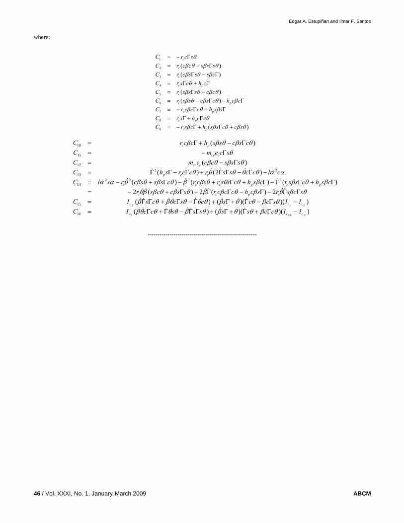
46 / Vol. XXXI, No. 1, January-March 2009 ABCM
where:
)(
)()(
)()(
9
8
7
6
5
4
3
2
1
θβθββθ
βθββθβθβ
θβθβθ
βθβθβθβ
θ
sccsshcsrCcchsrC
sshccsrCcchcscssrC
ccsssrCchcsrC
cssscrCsssccrC
scrC
pc
pc
pc
pc
c
pc
c
c
c
+Γ+Γ−=Γ+Γ=
Γ+Γ−=Γ−Γ−=
−Γ=Γ+Γ=
Γ−Γ=Γ−=
Γ−=
))()(()())()(()(
2)(2)(2)()()(
)2()()(
)(
016
15
222214
2213
12
11
10
XZY
ZYX
ccc
ccc
cpcc
pcpccc
ccp
ccr
ccr
pc
IIccsssssccICIIsccscsccsICscsrschcccrssccsr
cshcssrcshcssrscrcssscrslCclccssrccrshC
sssccemCscemC
cscsshccrC
−Γ+Γ+Γ+ΓΓ−Γ+Γ=−Γ−Γ+Γ+Γ−Γ+ΓΓ=ΓΓ−Γ−ΓΓ+Γ+−=
Γ+ΓΓ−Γ+Γ+−Γ+−=−Γ−ΓΓ+Γ−ΓΓ=
Γ−=Γ−=
Γ−+Γ=
θβθθβθβθθθθβθβθθβθθθθβθβ
θβθβθββθβθββθβθββθθθββθβθβθαα
ααθθθθθθβθβ
θθβθββ
&&&&&&&&&&
&&&&&&&&&&
&&&&&&
&&&&
&&&&&
-------------------------------------------------------