Modelling health care costs: practical examples and applications Andrew Briggs Philip Clarke...
28
Modelling health care costs: practical examples and applications Andrew Briggs Philip Clarke University of Oxford & Daniel Polsky Henry Glick University of Pennsylvania
-
date post
22-Dec-2015 -
Category
Documents
-
view
215 -
download
1
Transcript of Modelling health care costs: practical examples and applications Andrew Briggs Philip Clarke...

Modelling health care costs: practical examples and applications
Andrew Briggs
Philip Clarke
University of Oxford
&
Daniel Polsky
Henry Glick
University of Pennsylvania

Modelling health care costs:Presentation overview
• Statement of problem• Examples of cost distributions
– Overall– By treatment group
• Testing cost differences– Raw scale– Transformations– Back transformation
• Multivariate analysis– Raw scale– Transformation
• Summary/future directions
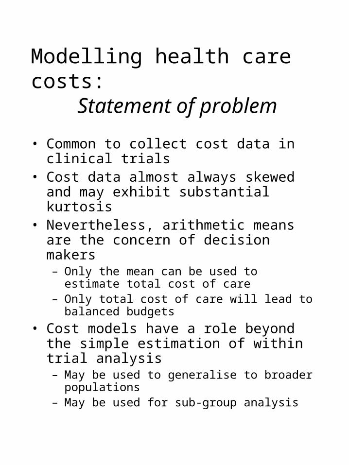
Modelling health care costs:Statement of problem
• Common to collect cost data in clinical trials
• Cost data almost always skewed and may exhibit substantial kurtosis
• Nevertheless, arithmetic means are the concern of decision makers– Only the mean can be used to estimate total
cost of care– Only total cost of care will lead to balanced
budgets
• Cost models have a role beyond the simple estimation of within trial analysis– May be used to generalise to broader
populations– May be used for sub-group analysis

Modelling health care costs:Examples of cost distributions
1.BOAES
Fra
ctio
n
Cost0 5000 10000 15000
0
.2
.4
.6
2.UKPDS
Fra
ctio
n
cost0 500 1000 1500 2000 2500
0
.2
.4
.6

Modelling health care costs:Examples of cost distributions
3.ACT
Fra
ctio
n
Cost0 100000 200000 300000
0
.1
.2
4.Dan
Fra
ctio
n
Cost0 100000 200000
0
.2
.4
.6
.8

Modelling health care costs:Examples of cost distributions
5.SAH
Fra
ctio
n
Cost0 100000 200000
0
.1
.2
.3
6.HG
Fra
ctio
n
Cost0 25000 50000 75000100000
0
.1
.2

Modelling health care costs:Cost distributions by treatment
1.BOAES: control group
Fra
ctio
n
Cost0 5000 10000 15000
0
.2
.4
.6
1.BOAES: treatment group
Fra
ctio
n
Cost0 5000 10000 15000
0
.2
.4
.6

Modelling health care costs:Cost distributions by treatment
2.UKPDS: control group
Fra
ctio
n
cost0 500 1000 1500 2000 2500
0
.2
.4
.6
2.UKPDS: treatment group
Fra
ctio
n
cost0 500 1000 1500 2000 2500
0
.2
.4
.6

Modelling health care costs:Cost distributions by treatment
3.ACT: control group
Fra
ctio
n
Cost0 100000 200000 300000
0
.1
.2
.3
3.ACT: treatment group
Fra
ctio
n
Cost0 100000 200000 300000
0
.1
.2
.3

Modelling health care costs:Cost distributions by treatment
4.Dan: control group
Fra
ctio
n
Cost0 100000 200000
0
.2
.4
.6
.8
4.Dan: treatment group
Fra
ctio
n
Cost0 100000 200000
0
.2
.4
.6
.8

Modelling health care costs:Cost distributions by treatment
5.SAH: control group
Fra
ctio
n
Cost0 100000 200000
0
.1
.2
.3
5.SAH: treatment group
Fra
ctio
n
Cost0 100000 200000
0
.1
.2
.3

Modelling health care costs:Cost distributions by treatment
6.HG: control group
Fra
ctio
n
Cost0 25000 50000 75000100000
0
.1
.2
6.HG: treatment group
Fra
ctio
n
Cost0 25000 50000 75000100000
0
.1
.2
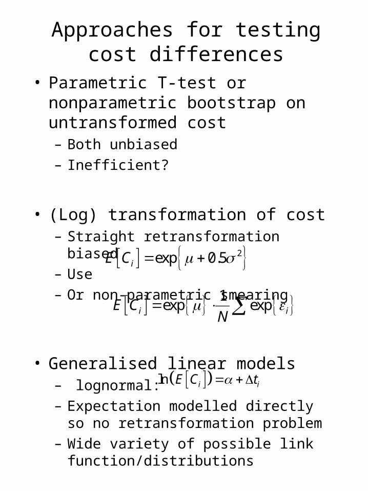
Approaches for testing cost differences
• Parametric T-test or nonparametric bootstrap on untransformed cost– Both unbiased
– Inefficient?
• (Log) transformation of cost– Straight retransformation biased
– Use
– Or non-parametric smearing
• Generalised linear models– lognormal:
– Expectation modelled directly so no retransformation problem
– Wide variety of possible link function/distributions
2exp 0.5iE C
ln i iE C t
1exp expi iE C
N

Zhou’s test based on log normality
• Special case of homogeneity of log variances – test of geometric means is equivalent to test of arithmetic means
• By symmetry: for special case of homogeneity of log means – test of equality of log variances is equivalent to test of arithmetic means?
• Zhou’s proposed test combines the two
2 20 1 1 0 0
2 20 1 1 0 0
2 20 1 1 0 0
2 20 1 0 1 1
: exp 0.5 exp 0.5
: 0.5 0.5
: 0.5 0.5 0
: 0 .
H
H
H
H iff

P-values and confidence intervals for back-transformed cost differences
Dataset P-value Cost diff (95% CI)
1. BOAE
T-test: raw cost
Bootstrapped means
Zhou (bootstrap)
Log (smeared)
GLM: log link / normal
GLM: B-C link / normal
0.013
0.012
0.026
<0.001
0.019
0.019
149
149
107
212
149
149
(31 -
(44 -
(21 -
(146 -
(26 -
(26 -
267)
255)
191)
278)
259)
260)
2. UKPDS
T-test: raw cost
Bootstrapped means
Zhou (bootstrap)
Log (smeared)
GLM: log link / normal
GLM: B-C link / normal
0.971
0.938
0.988
0.165
0.971
0.971
0
0
0
5
0
0
(-8 -
(-8 -
(-14 -
(-2 -
(-8 -
(-8 -
8)
8)
12)
13)
8)
8)
3. ACT
T-test: raw cost
Bootstrapped means
Zhou (bootstrap)
Log (smeared)
GLM: log link / normal
GLM: B-C link / normal
0.179
0.172
0.005
0.393
0.185
0.182
-15,523
-15,523
-136,747
14,162
-15,523
-15,523
(-38,248 -
(-37,854 -
(-611,607 -
(-18,321 -
(-37,212 -
(-37,458 -
7,201)
6,665)
-21,014)
47,530)
7,790)
7,509)

P-values and confidence intervals for back-transformed cost differences
Dataset P-value Cost diff (95% CI)
4. DP
T-test: raw cost
Bootstrapped means
Zhou (bootstrap)
Log (smeared)
GLM: log link / normal
GLM: B-C link / normal
0.057
0.058
<0.001
<0.001
0.073
0.071
2,925
2,925
114,565
-8,589
2,925
2,925
(-91 -
(-97 -
(64,023 -
(-13,277 -
(-297 -
(270 -
5,940)
5,807)
194,871)
-4,413)
5,675)
5701)
5. SAH
T-test: raw cost
Bootstrapped means
Zhou (bootstrap)
Log (smeared)
GLM: log link / normal
GLM: B-C link / normal
0.236
0.230
0.119
0.004
0.243
0.244
-4,060
-4,060
-4,019
-6,701
-4,060
-4,060
(-10,795 -
(-10,836 -
(-9,429 -
(-11,128 -
(-10,506 -
(-10,484 -
2,675)
2,575)
2,170)
-2,229)
2,881)
2,909)
6. HG
T-test: raw cost
Bootstrapped means
Zhou (bootstrap)
Log (smeared)
GLM: log link / normal
GLM: B-C link / normal
0.077
0.080
0.468
0.024
0.081
0.081
2,353
2,353
1,258
2,891
2,353
2,353
(-259 -
(-200 -
(-1,873 -
(394 -
(-298 -
(-295 -
4,965)
4,959)
4,388)
5,397)
4,899)
4,903)

Approaches to model selection
• Examine fit using standard regression diagnostics– R2, normal probability plots etc.
– Summarises fit to observed data
• Test the predictive ability of the models directly– Ability to predict observations
not used in model fitting
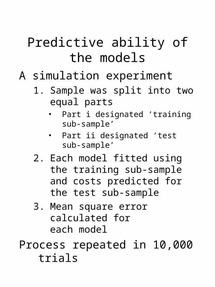
Predictive ability of the models
A simulation experiment 1. Sample was split into two equal parts
• Part i designated ‘training sub-sample’
• Part ii designated ‘test sub-sample’
2. Each model fitted using the training sub-sample and costs predicted for the test sub-sample
3. Mean square error calculated foreach model
Process repeated in 10,000 trials

Results of a simulation exercise
Model mean SE RMSE
OLS (cost) 10466 53 102OLS log(cost) no smearing 16072 226 127OLS log(cost) smeared 47432 1489 218OLS sqrt(cost) no smearing 10821 55 104OLS sqrt(cost) smearing 10441 54 102Poisson regression 11427 70 1072-part OLS (‘+’ve cost) 10467 53 1022-part OLS log(‘+’ve cost) no smearing
11298 54 1062-part OLS log(‘+’ve cost) smearing
11689 51 1082-part OLS sqrt(‘+’ve cost) no smearing
10616 55 1032-part OLS sqrt(‘+’ve cost) smearing
10429 54 102Tobit 10757 51 104
SE – estimated standard error of the mean
RMSE – root mean squared error
Mean squared error

P-values and confidence intervals for back-transformed cost differences
Dataset P-value Cost diff (95% CI)
1. BOAE
T-test: raw cost
Bootstrapped means
Zhou (bootstrap)
Log (smeared)
GLM: log link / normal
Covar Adj raw cost
Covar Adj: Log(smeared)
Covar Adj GLM: log
0.013
0.012
0.026
<0.001
0.019
0.
0.
0.
149
149
107
212
149
180
222
154
(31 -
(44 -
(21 -
(146 -
(26 -
(70 -
(126 -
(-48 -
267)
255)
191)
278)
259)
300)
338)
289)
2. UKPDS
T-test: raw cost
Bootstrapped means
Zhou (bootstrap)
Log (smeared)
GLM: log link / normal
Covar Adj raw cost
Covar Adj: Log(smeared)
Covar Adj GLM: log
0.971
0.938
0.988
0.165
0.971
0.
0.
0.
0
0
0
5
0
-1
0
-2
(-8 -
(-8 -
(-14 -
(-2 -
(-8 -
(-9 -
(-7 -
(-13 -
8)
8)
12)
13)
8)
6)
8)
7)
3. ACT
T-test: raw cost
Bootstrapped means
Zhou (bootstrap)
Log (smeared)
GLM: log link / normal
Covar Adj raw cost
Covar Adj: Log(smeared)
Covar Adj GLM: log
0.179
0.172
0.005
0.393
0.185
0.
0.
0.
-15,523
-15,523
-136,747
14,162
-15,523
-18,378
-12,602
-25,230
(-38,248 -
(-37,854 -
(-611,607 -
(-18,321 -
(-37,212 -
(-43,078 -
(-47,687 -
(-57,500 -
7,201)
6,665)
-21,014)
47,530)
7,790)
6,555)
24,271)
7,039)

P-values and confidence intervals for back-transformed cost differencesDataset P-value Cost diff (95% CI)
4. DP
T-test: raw cost
Bootstrapped means
Zhou (bootstrap)
Log (smeared)
GLM: log link / normal
Covar Adj raw cost
Covar Adj: Log(smeared)
Covar Adj GLM: log
0.057
0.058
<0.001
<0.001
0.073
0.
0.
0.
2,925
2,925
114,565
-8,589
2,925
3,078
3,649
3,364
(-91 -
(-97 -
(64,023 -
(-13,277 -
(-297 -
(125 -
(473 -
(-984 -
5,940)
5,807)
194,871)
-4,413)
5,675)
6,102)
6,924)
8,149)
5. SAH
T-test: raw cost
Bootstrapped means
Zhou (bootstrap)
Log (smeared)
GLM: log link / normal
Covar Adj raw cost
Covar Adj: Log(smeared)
Covar Adj GLM: log
0.236
0.230
0.119
0.004
0.243
0.
0.
0.
-4,060
-4,060
-4,019
-6,701
-4,060
-3,289
-4,036
-3,248
(-10,795 -
(-10,836 -
(-9,429 -
(-11,128 -
(-10,506 -
(-9,394 -
(-9,729 -
(-16,448 -
2,675)
2,575)
2,170)
-2,229)
2,881)
3,073)
1,680)
9,510)
6. HG
T-test: raw cost
Bootstrapped means
Zhou (bootstrap)
Log (smeared)
GLM: log link / normal
Covar Adj raw cost
Covar Adj: Log(smeared)
Covar Adj GLM: log
0.077
0.080
0.468
0.024
0.081
0.
0.
0.
2,353
2,353
1,258
2,891
2,353
1,759
1,772
1,540
(-259 -
(-200 -
(-1,873 -
(394 -
(-298 -
(-494 -
(-321 -
(-1,067 -
4,965)
4,959)
4,388)
5,397)
4,899)
4,068)
4,097)
4,132)

Modelling health care costs:Summary
• Different approaches to modelling health care cost can lead to quite different estimates
• Difficult to tell which is most appropriate• Transforming cost data can be more
efficient– GLM intuitive in modelling expectations– But modelling log cost better for heavy tails?
• Covariate adjustment can help precision and should be used whenever possible– Will be used to extrapolate beyond the data– Creates sub-group effects with transformed
models– Creates challenges for summarising
incremental cost across different covariate patterns

Modelling health care costs:Log cost distributions by treatment
1.BOAES: treatment group
Fra
ctio
n
Natural log of cost0 2 4 6 8 10
0
.1
.2
1.BOAES: control group
Fra
ctio
n
Natural log of cost0 2 4 6 8 10
0
.1
.2

Modelling health care costs:Log cost distributions by treatment
2.UKPDS: control group
Fra
ctio
n
Natural log of cost0 2 4 6 8 10
0
.1
.2
2.UKPDS: treatment group
Fra
ctio
n
Natural log of cost0 2 4 6 8 10
0
.1
.2

Modelling health care costs:Log cost distributions by treatment
3.ACT: control group
Fra
ctio
n
Natural log of cost0 2 4 6 8 10 12 14
0
.1
.2
3.ACT: treatment group
Fra
ctio
n
Natural log of cost0 2 4 6 8 10 12 14
0
.1
.2

Modelling health care costs:Log cost distributions by treatment
4.Dan: treatment group
Fra
ctio
n
Natural log of cost0 2 4 6 8 10 12 14
0
.1
.2
4.Dan: control group
Fra
ctio
n
Natural log of cost0 2 4 6 8 10 12 14
0
.1
.2

Modelling health care costs:Log cost distributions by treatment
5.SAH: control group
Fra
ctio
n
Natural log of cost0 2 4 6 8 10 12 14
0
.1
.2
5.SAH: treatment group
Fra
ctio
n
Natural log of cost0 2 4 6 8 10 12 14
0
.1
.2

Modelling health care costs:Log cost distributions by treatment
6.HG: treatment group
Fra
ctio
n
Natural log of cost0 2 4 6 8 10 12 14
0
.1
.2
6.HG: control group
Fra
ctio
n
Natural log of cost0 2 4 6 8 10 12 14
0
.1
.2


![1 BRIGGS LAW CORPORATION [FILE: 1593.60] Cory J. Briggs ...](https://static.fdocuments.in/doc/165x107/62143d16500e7a03e6034c04/1-briggs-law-corporation-file-159360-cory-j-briggs-.jpg)