Modelling Creep and Rate Effects in Soils - Home -...
104
Modelling Creep and Rate Effects in Soils Adel Albaba A dissertation submitted by Adel Albaba to the Department of Civil Engineering, University of Strathclyde, in part completion of the requirements for the MSc in Geotechnics. I, Adel Albaba, hereby state that this report is my own work and that all sources used are made explicit in the text 15,484 words August, 2012
Transcript of Modelling Creep and Rate Effects in Soils - Home -...

Modelling Creep and Rate Effects in Soils
Adel Albaba
A dissertation submitted by Adel Albaba to the Department of Civil Engineering, University of Strathclyde, in part completion
of the requirements for the MSc in Geotechnics.
I, Adel Albaba, hereby state that this report is my own work and that all sources used are made explicit in the text
15,484 words
August, 2012

i
Declaration of author’s rights
The copyright of this thesis belongs to the author under the terms of the United
Kingdom Copyright Acts as qualified by University of Strathclyde Regulation 3.49.
Due acknowledgement must always be made of the use of any material contained in,
or derived from, this thesis.

ii
Abstract
With more constructions being concentrated in densely populated areas, there is an
increasing need to construct geotechnical structures in problematic soils which
produce significant creep. Many properties of such soils (e.g. undrained shear
strength) have been found to be time-dependent. A lot of research work has been
related to creep and time-dependent behaviour of soils in the last three decades. Two
creep hypotheses have been presented in this work where, after experimental review,
hypothesis B was found to be more realistic.
The evolution of constitutive models has been briefly reviewed. The concepts and
theories which these models are based on were presented chronologically. Elasto-
viscoplastic models (creep and rate models) based on Perzyna’s (1963) theory were
discussed and their strengths and limitations were reviewed. Two Models were
considered for the simulations and comparisons: Modified Cam-clay model MCC
developed by Schofield and Burland (1968) and an elasto-viscoplastic model EVP.
The latter was proposed by Wheeler (2011) as a viscoplastic equivalent of the
famous MCC model to account for creep and rate-dependent behaviour.
The methodology was based on simulations, using MS Excel, of drained and
undrained conventional triaxial tests of a slightly overconsolidated soil sample with
soil constants that are representative of typical moderately high plasticity clay, such
as London Clay. The simulations were carried out with the two models MMC and
EVP in which different loading rates were chosen for the latter model together with
stress-controlled shearing and strain-controlled shearing.
Experimental data was presented to show how soils behave in real triaxial
experiments. By comparing these data with the simulation results, the importance of
including the viscoplastic behaviour of soils was demonstrated, where many
important properties of soils as (creep, influence of rate of loading on undrained
shear strength and etc.) were captured by the proposed EVP model.
Keywords: Creep, rate effects, time-dependency, soft soils, secondary
compression, constitutive modelling, elastoplasticity, elasto-
viscoplasticity

iii
Acknowledgments
The writing of this dissertation has been one of the most significant academic
challenges I have ever had to face. It would not have been possible to write it without
the help and support of the kind people around me, to only some of whom it is
possible to give particular mention here.
Above all, I would like to express my deepest gratitude to my advisor, Prof Simon
Wheeler, for his excellent guidance, caring and patience. His wisdom, knowledge
and commitment to the highest standards inspired and motivated me. I would also
like to thank the course director Prof Minna Karstunen for her useful notes
concerning soil modelling and numerical analysis. Her class on soil modelling
greatly helped me in developing my skills in this discipline.
I am most grateful to Dr. Jehad Hamad whom was my principal supporter towards
geotechnical engineering. I would not have been at this stage without his support. I
am also grateful to Ayman Nassar for his kind help with different soil modelling
aspects.
I would like to acknowledge the full financial support of Hani Alqadoumi
Scholarship Foundation (HQSF), especially the donors of this scholarship Mr.
Omar/Jawdat Shawwa who provided the financial support of this research.
Last, by no means least, I would like to thank my parents, brothers and sisters. They
were always supporting me and encouraging me with their best wishes.
For any errors or inadequacies that may remain in this work, of course, the
responsibility is entirely my own.
Adel Albaba
Glasgow, United Kingdom, August 2012
iv
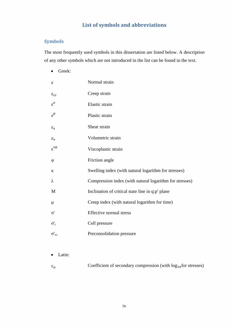
List of symbols and abbreviations
Symbols
The most frequently used symbols in this dissertation are listed below. A description
of any other symbols which are not introduced in the list can be found in the text.
• Greek:
ε Normal strain
εcr Creep strain
εe Elastic strain
εp Plastic strain
εs Shear strain
εv Volumetric strain
εvp Viscoplastic strain
φ Friction angle
κ Swelling index (with natural logarithm for stresses)
λ Compression index (with natural logarithm for stresses)
M Inclination of critical state line in q:p’ plane
μ Creep index (with natural logarithm for time)
σ' Effective normal stress
σ'r Cell pressure
σ'vc Preconsolidation pressure
• Latin:
cα Coefficient of secondary compression (with log10for stresses)
v
cc Compression index (with log10for stresses)
cu Undrained shear strength
dv/hi Nominal strain
e Void ratio
e Void ratio rate
E Young’s modulus
fs Static yield surface
Fd Dynamic yield surface
G Shear Modulus
K Bulk modulus
p Mean total stress
p′ Mean effective stress
q Deviatoric stress
u Pore water pressure

vi
Abbreviations
CD Consolidated-Drained triaxial test
CU Consolidated-Undrained triaxial test
CSL Critical state line
EOP End of primary consolidation
EVP Elasto-viscoplastic model proposed by (Wheeler, 2011)
MCC Modified Cam-clay model
NCL Normal compression line
OCR Overconsolidation ratio
SL Swelling line
URL Unloading-reloading line
UU Unconsolidated-Undrained triaxial test
YL Yield locus
vii
Contents
Declaration of author’s rights .................................................................................................... i
Abstract ..................................................................................................................................... ii
Acknowledgments .................................................................................................................... iii
List of symbols and abbreviations............................................................................................ iv
Symbols ................................................................................................................... iv
Abbreviations .......................................................................................................... vi
Chapter 1: Introduction .............................................................................................................. 1
Overview ....................................................................................................... 1 1.1
Aim of the research ....................................................................................... 3 1.2
Organisation of the dissertation ..................................................................... 3 1.3
Chapter 2: Literature review of creep and rate-dependency ...................................................... 5
Creep ............................................................................................................. 5 2.1
2.1.1 Creep theories......................................................................................... 5
2.1.2 Experimental work supporting creep hypotheses .................................. 8
Effect of rate of shearing ............................................................................. 14 2.2
Chapter 3: Literature review of soil modelling ........................................................................ 18
Elasticity ...................................................................................................... 19 3.1
Elastoplasticity ............................................................................................ 22 3.2
3.2.1 Uniaxial behaviour of a linear elastic-perfectly plastic material ......... 23
3.2.2 Uniaxial behaviour of a linear elastic-strain hardening plastic material
25
3.2.3 Uniaxial behaviour of a linear elastic-strain softening plastic material26
3.2.4 Elastic volumetric strains ..................................................................... 27
3.2.5 Plastic volumetric strains ..................................................................... 29
3.2.6 Plastic shear strains .............................................................................. 30
viii
3.2.7 Critical state line (CSL) ....................................................................... 32
Viscoplasticity ............................................................................................. 34 3.3
3.3.1 Overstress theory .................................................................................. 34
3.3.2 Viscoplastic Soil Models ..................................................................... 35
Chapter 4: MCC and EVP Models ........................................................................................... 40
Modified Cam-Clay MCC Model ............................................................... 40 4.1
4.1.1 Elastic stress-strain relations ................................................................ 41
4.1.2 Yield surface ........................................................................................ 41
4.1.3 Flow rule .............................................................................................. 41
4.1.4 Hardening Law ..................................................................................... 42
4.1.5 Advantages and limitations .................................................................. 43
Elasto-viscoplastic (EVP) Model ................................................................ 44 4.2
4.2.1 Elastic stress-strain relations ................................................................ 44
4.2.2 Viscoplastic Curve ............................................................................... 44
4.2.3 Hardening Law ..................................................................................... 45
4.2.4 Viscoplastic relation ............................................................................. 46
4.2.5 Flow rule .............................................................................................. 47
4.2.6 EVP Advantages over MCC ................................................................ 47
Chapter 5: Methodology .......................................................................................................... 48
Triaxial compression test ............................................................................. 48 5.1
5.1.1 Consolidated-Drained test (CD) ........................................................... 49
5.1.2 Consolidated-Undrained test (CU) ....................................................... 49
5.1.3 Consolidated-Undrained test (UU) ...................................................... 49
5.1.4 Testing procedure ................................................................................. 49
5.1.5 Data presentation .................................................................................. 51
Isotropic Loading ........................................................................................ 51 5.2
ix
5.2.1 Calculation method .............................................................................. 53
Drained Shearing ......................................................................................... 53 5.3
5.3.1 Calculation method .............................................................................. 54
Undrained Shearing ..................................................................................... 56 5.4
5.4.1 Calculation method .............................................................................. 56
Chapter 6: Simulations and Results ......................................................................................... 58
Isotropic loading .......................................................................................... 59 6.1
Drained shearing .......................................................................................... 59 6.2
Undrained shearing ...................................................................................... 65 6.3
Discussion ................................................................................................... 70 6.4
6.4.1 Creep effect during isotropic loading ................................................... 70
6.4.2 Soil stiffness ......................................................................................... 71
6.4.3 Undrained shear strength...................................................................... 71
6.4.4 Pore water pressure generation ............................................................ 72
Chapter 7: Conclusions and recommendations ........................................................................ 74
Conclusions ................................................................................................. 74 7.1
Recommendations for further work............................................................. 75 7.2
References ................................................................................................................................ 76
Appendix A: Isotropic Loading Calculations .......................................................................... 81
A.1 EVP model: ................................................................................................. 81
Appendix B: Drained Shearing Calculations ........................................................................... 83
B.1 MCC model – stress controlled: .................................................................. 83
B.2 EVP model – stress controlled: ................................................................... 85
B.3 EVP model – strain controlled: ................................................................... 87
Appendix C: Undrained Shearing Calculations ....................................................................... 89
C.1 MCC model: ................................................................................................ 89
x
C.2 EVP model – stress controlled: ................................................................... 90
C.3 EVP model – strain controlled: ................................................................... 92
1 | P a g e
Chapter 1: Introduction 1
Overview 1.1
In geotechnical engineering, constitutive modelling has been an active topic for
research since the 1960’s. One of the most commonly used theories for formulation
of constitutive models is elastoplasticity with the Modified Cam-clay model MCC
(Roscoe and Burland, 1968) one of the earliest and most widely used of elastoplastic
models. The elastoplastic models capture important features of soil behaviour, and
assume that both elastic and plastic components of strains are only dependent on
increments of effective stresses, regardless of the rate at which these effective
stresses are applied. As a result, such models do not account for creep and rate-
dependency. However, creep and rate-dependency are important factors, particularly
when dealing with soft soils characterised by low shear strength and high water
content. Such characteristics can be captured with elasto-viscoplastic models, which
are based on the theory of elasto-viscoplasticity, first proposed by Perzyna (1963,
1966). Elasto-viscoplastic constitutive models provide a suitable solution for
including the effects of creep and rate-dependency.
A well-known historical case of creep on soft soil is the uneven settlement of the
leaning tower of Pisa (Figure 1-1a) in Italy (Havel, 2004). Construction of the tower
started in 1173 but was ceased for unknown reasons in 1178. Later studies showed
that the underlying soil would have collapsed had the construction continued without
a pause, as it would not have been able to withstand more loading at that time. The
construction started again in 1278 and completely finished in 1370 with a height of
58 m measured from the foundation and 54.58 m above the ground surface. The
foundation’s soil is a sandy soil with lenses of clay where creep deformations took
place. These clayey lenses were present under one side of the tower which resulted in
settling with an average of 1.5 m (Figure 1-1b) and continuous tilting (Figure 1-2)
with a maximum recoded angle of 5.5ᴼ in 1993 (Marchi et al., 2011) at which
stabilisation work started.
From this example, it can be seen how essential it is for designers to study creep
deformations in order to predict the in-situ creep behaviour.

2 | P a g e
Figure 1-1 (a) Tower of Pisa section with the soil layers below it; (b) Mean settlement of the
tower developing with mass and time (Havel, 2004)
Figure 1-2 Pisa tower field data (Marchi et al., 2011)
3 | P a g e
Problems of continuous settlements at constant stresses such as Pisa tower case is of
a significant importance as they might result in serviceability failure of the structure.
Aim of the research 1.2
The project involves simulations performed at stress-point level representing
laboratory tests such as drained and undrained triaxial tests under stress-controlled
and strain-controlled loading. Two models will be used for the simulations: the
Modified Cam-clay model MCC, which represent a conventional elastoplastic
constitutive model; and an equivalent elasto-viscoplastic model EVP proposed by
Wheeler (2011). The simulations are performed using MS Excel. The aim is to
investigate the implications of including and excluding creep and rate-dependency
effects in constitutive modelling of soils.
Organisation of the dissertation 1.3
A brief description of the following chapters included in this dissertation can be
summarized as follows:
Chapter 2 presents literature review of creep and time dependency where two
different creep hypotheses are discussed, critically reviewed and compared with
experimental results. The time-dependent behaviour of soils is then discussed along
with experimental soil data that proves this behaviour.
Chapter 3 presents different theories of soil behaviour (elasticity, elastoplasticity and
elasto-viscoplasticity) along with the evolution of different constitutive models
where their drawbacks and strengths are discussed.
Chapter 4 concentrates specifically on the equations used for the two models under
consideration: MCC and EVP. The strengths and limitations are then presented
showing the advantages of the EVP model over the MCC.
Chapter 5 presents the methodology in which brief explanation is given for triaxial
test along with specific explanation of the calculation methods of each type of
simulation (isotropic loading, drained sharing and undrained shearing).

4 | P a g e
Chapter 6 contains the results of the simulations and qualitative comparisons with
real soil behaviour in terms of creep effect under isotropic loading, soil stiffness,
undrained shear strength and pore water pressure generation.
Chapter 7 presents conclusions and recommendations for further work on the
proposed EVP model. Samples of tables of simulations are listed in the appendices.
5 | P a g e
Chapter 0: Literature review of creep and rate-dependency 2
Creep 2.1
Fine-grained materials are complex in their nature and behaviour. The creep
behaviour is traditionally defined as continuous deformations with constant effective
stresses which are influenced by many factors such as stress history, change in
temperature, biochemical environment and transformations. Clayey soils, in
comparison with sandy soils, display large creep deformations as previously seen in
Pisa tower case.
Creep problem started to be under observation with the intensive revolution in the
building activities especially after observing large prolonged deformations of the
structures. This came after sorting out the definition of effective stress in the 1920’s
by Terzaghi. During the last centuries as well as the last few years, creep
deformations in soft soils have been one of the most important problems of soil
mechanics.
2.1.1 Creep theories
Traditionally, deformations of foundations on saturated soils have been divided into
three types (Smoltczyk, 2002):
1. Immediate settlement: This takes place immediately after the application of
the load which involves shear deformations under constant volume.
2. Consolidation settlement: in which deformations are caused by the dissipation
of the excess pore pressure (i.e. effectives stresses are changing), where both
volumetric and shear deformations are observed.
3. Creep settlement: a time-dependent settlement resulting from the
readjustment of particle contacts at essentially constant effective stresses
which involves shear and volumetric strains.
Estimation of creep settlement is the least well-developed settlement among all types
of deformation (Smoltczyk, 2002). The early work on creep concentrated mainly on
results of 1-D straining in oedometer test as well as field behaviour of horizontal
layers of soils under uniform loading.
6 | P a g e
As a complex phenomenon with many factors affecting it, several creep theories
have been developed to describe creep behaviour. The theories concentrate mainly
on two issues: the equations used to relate creep strain, stress and time:
ε = f(σ, t) (2.1)
and how to describe the creep phenomenon (when creep deformations of soil start).
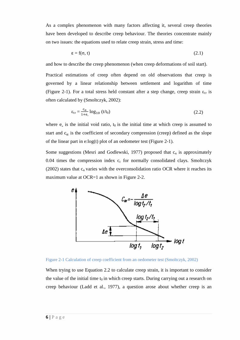
Practical estimations of creep often depend on old observations that creep is
governed by a linear relationship between settlement and logarithm of time
(Figure 2-1). For a total stress held constant after a step change, creep strain εcr is
often calculated by (Smoltczyk, 2002):
εcr = cα1+e˳
log10 (t/t0) (2.2)
where e˳ is the initial void ratio, t0 is the initial time at which creep is assumed to
start and cα is the coefficient of secondary compression (creep) defined as the slope
of the linear part in e:log(t) plot of an oedometer test (Figure 2-1).
Some suggestions (Mesri and Godlewski, 1977) proposed that cα is approximately
0.04 times the compression index cc for normally consolidated clays. Smoltczyk
(2002) states that cα varies with the overconsolidation ratio OCR where it reaches its
maximum value at OCR=1 as shown in Figure 2-2.
Figure 2-1 Calculation of creep coefficient from an oedometer test (Smoltczyk, 2002)
When trying to use Equation 2.2 to calculate creep strain, it is important to consider
the value of the initial time t0 in which creep starts. During carrying out a research on
creep behaviour (Ladd et al., 1977), a question arose about whether creep is an

7 | P a g e
independent phenomenon of primary consolidation. If this is true, the time to the end
of primary consolidation EOP (And hence t0) depends on the thickness of soil layers.
Such a consideration led to two opposing hypotheses (A and B) concerning sample’s
thickness effect and when does creep actually starts.
Figure 2-2 The variation of Cα with OCR (Smoltczyk, 2002)
Hypothesis A (Mesri and Godlewski, 1977) assumes that creep occurs only after the
end of primary consolidation and the strain at EOP is independent of the
consolidation period (i.e. the thickness of the soil layer). In contrast, Hypothesis B
(Leroueil, 1994) assumes the secondary compression to take place simultaneously
with the primary consolidation with an increasing EOP strain with increasing soil
layers thickness (increasing consolidation period).
Early researchers (Šuklje, 1957), (Bjerrum, 1967) and (Janbu, 1696) assumed that
any combination of strain, stress and strain rate is unique in both primary and
secondary consolidation. Such assumption implies that, for 1-D straining, creep rate
at any point is given by the current effective stress and void ratio. These assumptions
were advocated and used in further research (Vermeer and Neher, 1999), (Leroueil,
2006), (Karim et al., 2010) and (Nash, 2010) as the basis for supporting hypothesis
B. Others (Aboshi, 1973); (Mesri and Godlewski, 1977) and (Mesri, 2003) supported
hypothesis A by experimentally finding that EOP void ratio is independent of the
consolidation period. Such findings supported hypothesis A as they were wrongly
presented as will be discussed in section 2.1.2.

8 | P a g e
When comparing between the two hypotheses, only little difference is observed
between the two when implementing standard laboratory incremental load
consolidation tests using thin specimen where the time required for consolidation
may last for orders of minutes which minimises the difference between the two
hypotheses. In in-situ situations, very significant difference (Figure 2-3) is observed
when predicting field consolidation settlement for thick layers with very low
permeability requiring long durations (sometimes several decades) for the dissipation
of excess pore pressure (Ladd and DeGroot, 2003). Thus, it is of a great importance
to understand the effect of the time scale between the thin laboratory specimens and
thick in-situ layers. How to account for this difference has been an active scientific
debate among researchers (Leroueil, 2006) and (Mesri, 2003).
Figure 2-3 Hypotheses A and B for consolidation of clay layers with different thickness
(Ladd et al., 1977)
2.1.2 Experimental work supporting creep hypotheses
Degago and his colleagues (2010) critically reviewed previous experimental studies
that advocated either hypotheses A or B using the isotach concept which was
proposed by Šuklje in 1957. The concept describes the rate effects on the clayey soil
compressibility stating that the rate of change of void ratio is uniquely related to the
current stress state and void ratio. Figure 2-4 describes the principle of isotach in
which several broken lines represent different constant void ratio rates ej+n. This
implies the existence of a unique combination of e, σv and e for the whole process of

9 | P a g e
soil compressibility (primary and secondary consolidation) which supports
hypothesis B.
Figure 2-4 Illustration of the isotach concept (Degago et al., 2010)
Degago et al. (2010) performed an incremental oedometer test on two specimens
with different thicknesses (1 cm and 10 cm). The preconsolidation pressure σvc was
100 kPa in which drainage was allowed to take place until 99% of the initial pore
pressure has dissipated. The nominal strain dv/hi was used to in presenting the data
which is the normalisation of the vertical deformation dv by the initial height hi.
When plotting the vertical strain against the vertical effective stress (Figure 2-5), it
can be seen how the EOP point for each load increment can be identified for each
specimen. When connecting the EOP points, a reference isotach is defined for a
specific EOP strain rate. For loads before the preconsolidation pressure, the soil
behaves elastically and no difference between the two specimens is observed as
creep contribution is insignificant. However, significant difference starts to be
observed when approaching the preconsolidation pressure (100 kPa) where the
difference between the two specimens is marked. For stresses below the initial σvc,

10 | P a g e
the two specimens had similar creep rate. When exceeding the initial σ vc, different
EOP strain is observed due to the difference in consolidation periods. However, for
stress increments in the normally consolidated regime, the thin specimen will have
faster creep deformations for a shorter time while the other specimen will have lower
creep deformations for longer time. Eventually, the incremental EOP strains will be
the same for both specimens.
Figure 2-5 EOP paths (curved lines) followed by two soil specimens with different thickness
and the corresponding isotach lines (straight lines) of EOP state (Degago et al., 2010)
In order to examine the response of the two specimens beyond σ vc, both specimens
were incrementally loaded with an EOP condition of 50 kPa ensuring an
overconsolidated state and the simulation started at the same effective stress:void
ratio state. Next, a load increment of 100 kPa was applied and the two specimens
were left to creep for 100 days. Figure 2-6 shows the two specimens starting from the
same point but end up having different EOP nominal strains where it is larger for the
thick specimen. However, eventually, the two specimens converge to the same line
of nominal strain:time plot.
The next simulation was to load the two specimens to a higher stress (200 kPa) in
which they were afterwards left to creep for 100 days.
11 | P a g e
Figure 2-6 The change in nominal stain with time when exceeding the initial σvc (loading
from 50 kPa to 150 kPa) (Degago et al., 2010)
When reaching the initial σvc, nominal strains become different for each specimen
marking the start of the next stress increment. After applying the additional 100 kPa,
each specimen yields at different EOP void ratio which increases with the specimen
thickness. Eventually, after creeping for long time, the deformation curves of the two
specimens converge to the same line (Figure 2-7). The results of Degago et al. (2010)
experiment strongly support hypothesis B.
Choi (1982) and Feng (1991) have conducted tests on specimens of 127 mm and 508
mm where they used the results to advocate hypothesis A. However, Degago et al.
(2009) critically reviewed their work concluding that after re-interpretation of the
test’s findings of Choi (1982) and Feng (1991), using consistent EOP criteria, the
new results support hypothesis B.
Aboshi (1973) conducted carefully designed laboratory and field tests on different
specimens of Hiroshima Bay with different sizes.
A preliminary consolidation stage of up to 20 kPa was limited by the end of primary
consolidation to assure a normally consolidated regime. Next, a one loading step was
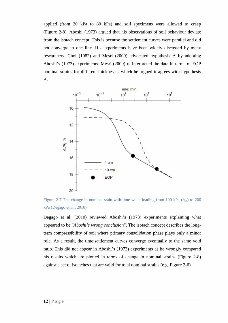
12 | P a g e
applied (from 20 kPa to 80 kPa) and soil specimens were allowed to creep
(Figure 2-8). Aboshi (1973) argued that his observations of soil behaviour deviate
from the isotach concept. This is because the settlement curves were parallel and did
not converge to one line. His experiments have been widely discussed by many
researchers. Choi (1982) and Mesri (2009) advocated hypothesis A by adopting
Aboshi’s (1973) experiments. Mesri (2009) re-interpreted the data in terms of EOP
nominal strains for different thicknesses which he argued it agrees with hypothesis
A.
Figure 2-7 The change in nominal stain with time when loading from 100 kPa (σvc) to 200
kPa (Degago et al., 2010)
Degago et al. (2010) reviewed Aboshi’s (1973) experiments explaining what
appeared to be “Aboshi’s wrong conclusion”. The isotach concept describes the long-
term compressibility of soil where primary consolidation phase plays only a minor
rule. As a result, the time:settlement curves converge eventually to the same void
ratio. This did not appear in Aboshi’s (1973) experiments as he wrongly compared
his results which are plotted in terms of change in nominal strains (Figure 2-8)
against a set of isotaches that are valid for total nominal strains (e.g. Figure 2-6).

13 | P a g e
Figure 2-8 Consolidation test on samples of different thickness from Hiroshima Bay clay
(Aboshi, 1973)
Konovalov & Bezvolev (2005) concluded, after conducting specially designed EOP
consolidation tests (Figure 2-9), that disregarding the effect of void ratio-stress
history of a soil has a sequence of giving a misleading picture.
From all previously reviewed studies, it can be concluded that most of the
consolidation test results agree with the isotach concept which supports hypothesis
B. Hypothesis A is wrong for stress increments exceeding the initial of value σ vc in
addition to stress increments in which the whole stress-strain history is taken into
consideration (Degago et al., 2010).
Furthermore, hypothesis B can be advocated by considering an in-situ example of a
soil element in two soil layers: 1 m and 10 metre thick. Hypothesis A assumes that
creep will only occur by the end of primary consolidation. For EOP, It might take
one year for the first layer to start creeping while it might take 10 years for the
second. However, as far as this soil element is concerned, it should behave exactly
the same in the two cases which deviate from Hypothesis A. In other words, if a soil
element was loaded from 0 to 99 kPa in one step and then loaded from 99 kPa to 100
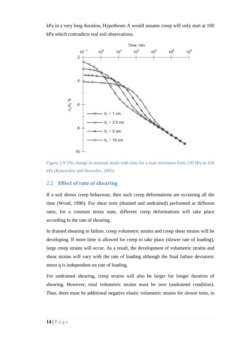
14 | P a g e
kPa in a very long duration, Hypotheses A would assume creep will only start at 100
kPa which contradicts real soil observations.
Figure 2-9 The change in nominal strain with time for a load increment from 230 kPa to 430
kPa (Konovalov and Bezvolev, 2005)
Effect of rate of shearing 2.2
If a soil shows creep behaviour, then such creep deformations are occurring all the
time (Wood, 1990). For shear tests (drained and undrained) performed at different
rates, for a constant stress state, different creep deformations will take place
according to the rate of shearing.
In drained shearing to failure, creep volumetric strains and creep shear strains will be
developing. If more time is allowed for creep to take place (slower rate of loading),
large creep strains will occur. As a result, the development of volumetric strains and
shear strains will vary with the rate of loading although the final failure deviatoric
stress q is independent on rate of loading.
For undrained shearing, creep strains will also be larger for longer duration of
shearing. However, total volumetric strains must be zero (undrained condition).
Thus, there must be additional negative elastic volumetric strains for slower tests, to
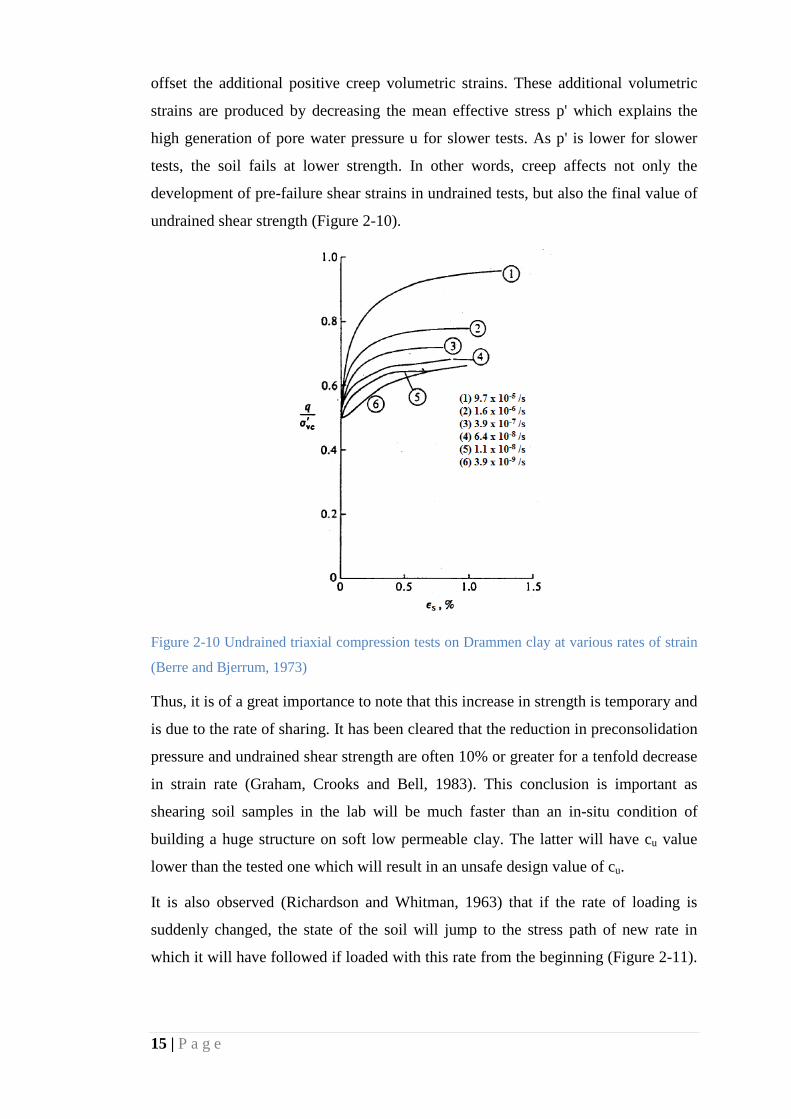
15 | P a g e
offset the additional positive creep volumetric strains. These additional volumetric
strains are produced by decreasing the mean effective stress p' which explains the
high generation of pore water pressure u for slower tests. As p' is lower for slower
tests, the soil fails at lower strength. In other words, creep affects not only the
development of pre-failure shear strains in undrained tests, but also the final value of
undrained shear strength (Figure 2-10).
Figure 2-10 Undrained triaxial compression tests on Drammen clay at various rates of strain
(Berre and Bjerrum, 1973)
Thus, it is of a great importance to note that this increase in strength is temporary and
is due to the rate of sharing. It has been cleared that the reduction in preconsolidation
pressure and undrained shear strength are often 10% or greater for a tenfold decrease
in strain rate (Graham, Crooks and Bell, 1983). This conclusion is important as
shearing soil samples in the lab will be much faster than an in-situ condition of
building a huge structure on soft low permeable clay. The latter will have cu value
lower than the tested one which will result in an unsafe design value of cu.
It is also observed (Richardson and Whitman, 1963) that if the rate of loading is
suddenly changed, the state of the soil will jump to the stress path of new rate in
which it will have followed if loaded with this rate from the beginning (Figure 2-11).

16 | P a g e
Furthermore, if an oedometer compression test is performed (Figure 2-12) with a fast
rate of loading (AB) and then stopped, creep deformations occur with a rate that
gradually falls with time (BC) shifting the soil state to lower v:ln(p') curves. If the
soil is then reloaded (CDE), an apparent overconsolidation behaviour will be
observed as the state of the soil has been taken to point C below the
stress:deformation curve for the particular rate of loading. An apparent
preconsolidation pressure will be assigned to point D even though the soil has not
been loaded to effective stresses higher than this at points B and C. This also has an
effect on the yield surface.
Figure 2-11 Stress-strain curves for triaxial compression tests with step-changed stain rate
and relaxation procedure (Graham, Crooks and Bell, 1983)

17 | P a g e
Figure 2-12 Effect of rate of strain on one-dimensional compression of clay (Wood, 1990)
The size of the yield surface is dependent on the preconsolidation pressure (as will be
discussed in Chapter 3). Thus, the size of the yield surface is dependent on the rate of
which the soil is deforming (Tavenas et al., 1978). Experimental data with different
duration of loading increment shows that with a decrease in the rate of loading, the
size of the yield surface decreases (Figure 2-13).
Figure 2-13 Effect of duration of load increment on the position of the yield surface in
triaxial tests on St. Alban clay (Wood, 1990)

18 | P a g e
Chapter 3: Literature review of soil modelling 3
In Geotechnical Engineering, soil modelling is concerned with analysing, predicting
and understanding the behaviour of real soil. However, it is nearly impossible to
perfectly model this behaviour. This is because, unlike mechanical and structural
engineering, the material under study (soil) is not a man-made material where
properties are specified and controlled (steel, concrete and other manufactured
materials). In addition, when subjected to stresses, soil behaves non-linearly and
shows anisotropy and time-dependent behaviour. Soil behaviour depends on a
number of issues (Potts et al., 2002), in which the more significant are the soil
composition (e.g. percentage of fine-grained particles), the loading history
(overconsolidation ratio, stress path, etc.) and drainage condition. This complexity of
soil behaviour was the reason for the existence of many soil models proposed by
different researchers. This non-linear behaviour is observed well below failure
condition. (Sekiguchi, 1977) (Borja and Kavazanjian, 1985)
Each soil model has specific advantages and limitations. When evaluating a soil
model, a balance is required between three basic criteria (Bažant, 1985):
1. The theoretical evaluation of the model and how this conforms to the
theoretical requirements of continuity, stability and uniqueness (basic
principles of continuum mechanics).
2. Experimental evaluation of the model and how the model fits with the variety
of available experimental data as well as how the model’s parameters can be
determined from standard tests.
3. The numerical and computational evaluation of the model and how the model
can be used in computer calculations.
Researchers made an increasing effort over the last five decades to develop a more
comprehensive description of soil behaviour along with the development of
numerical methods and the mutual influence between them. There is not yet a full
agreement among researchers about the different models that have been proposed.
These models vary between Elastic (e.g. Duncan and Chang, 1970), Elastoplastic
(e.g. Roscoe and Burland, 1968) and Elasto-viscoplastic models (e.g. Sekiguchi,

19 | P a g e
1977; Adachi and Oka, 1982 and Borja and Kavazanjian, 1985). These models vary
in the level of complexity and sophistication according to the three previously
mentioned criteria.
Nowadays, the user of any finite element packages (e.g. PLAXIS) can choose
between different soil models which until a few years ago were available only for
researchers.
Elasticity 3.1
The material is said to be elastic and follows Hook’s law if the stress-strain change is
reversible. It has been found from practical testing of soils that the soil behaves
elastically over some part of its stress-strain curve. Elasticity is divided into isotropic
and non-isotropic elasticity. Effect of anisotropy is out of the scope of this
dissertation.
For the soil to be isotropic, two elastic constants are required to describe its
behaviour: Young’s modulus E’ and Poisson’s ratio ν’. These two constants are the
most widely understood ones as they can be directly observed in experiments using
conventional triaxial tests (Figure 3-1). However, it is more convenient to represent
isotropic elastic soil in terms of the bulk modulus K’ (Equation 3.1) and shear
modulus G (Equation 3.2). These two parameters divide the elastic strains into
volumetric (change in size) and shear (change in shape or distortion). For example,
when soil deforms under constant volume (undrained shearing), deformation take
place in the form of distortion without any volume change.
K’ is related to E’ and ν’ by:
K’ = E’3(1−2ν’)
(3.1)
and G’ is related to E and ν by
G’ = E’2(1+ν’)
(3.2)
Using K’ and G’, the stress:strain relationship matrix become:
�dεvdεs
� = �1/K’ 00 1/3G’� �
dp dq� (3.3)
20 | P a g e
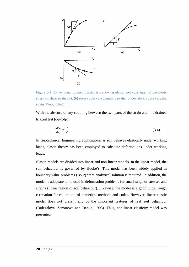
Figure 3-1 Conventional drained triaxial test showing elastic soil constants: (a) deviatoric
stress vs. shear strain plot; (b) shear strain vs. volumetric strain; (c) deviatoric stress vs. axial
strain (Wood, 1990) (Adachi and Oka, 1982) (Duncan and Chang, 1970)
With the absence of any coupling between the two parts of the strain and in a drained
triaxial test (dq=3dp):
dεvdεs
= G’K’
(3.4)
In Geotechnical Engineering applications, as soil behaves elastically under working
loads, elastic theory has been employed to calculate deformations under working
loads.
Elastic models are divided into linear and non-linear models. In the linear model, the
soil behaviour is governed by Hooke’s. This model has been widely applied in
boundary value problems (BVP) were analytical solution is required. In addition, the
model is adequate to be used in deformation problems for small range of stresses and
strains (linear region of soil behaviour). Likewise, the model is a good initial rough
estimation for calibration of numerical methods and codes. However, linear elastic
model does not present any of the important features of real soil behaviour
(Dolezalova, Zemanova and Danko, 1998). Thus, non-linear elasticity model was
presented.
21 | P a g e
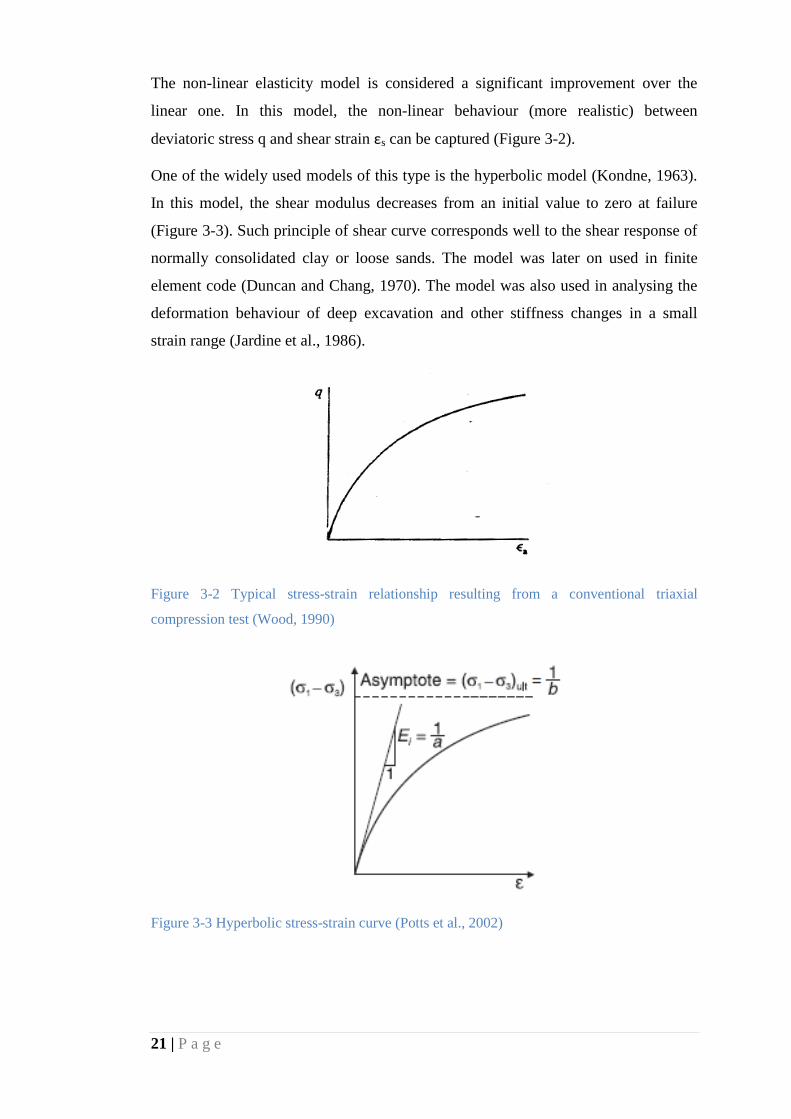
The non-linear elasticity model is considered a significant improvement over the
linear one. In this model, the non-linear behaviour (more realistic) between
deviatoric stress q and shear strain εs can be captured (Figure 3-2).
One of the widely used models of this type is the hyperbolic model (Kondne, 1963).
In this model, the shear modulus decreases from an initial value to zero at failure
(Figure 3-3). Such principle of shear curve corresponds well to the shear response of
normally consolidated clay or loose sands. The model was later on used in finite
element code (Duncan and Chang, 1970). The model was also used in analysing the
deformation behaviour of deep excavation and other stiffness changes in a small
strain range (Jardine et al., 1986).
Figure 3-2 Typical stress-strain relationship resulting from a conventional triaxial
compression test (Wood, 1990)
Figure 3-3 Hyperbolic stress-strain curve (Potts et al., 2002)

22 | P a g e
Non-linear elastic models can well represent monotonic curves of experimentally
measured stress-strain relations for specific loading path. However, these models
mainly focus on the soil response during one particular stress path and do not take
into account other important features such as stress paths dependence, volume
change during shearing and the differences in loading and unloading responses. In
addition, unlike linear elastic models, the non-linear elastic model lacks proper
theoretical background.
Elastoplasticity 3.2
Plasticity allows limiting stress ranges, enabling dilatancy and also, to a certain
degree, enabling hysteretic behaviour to be captured. It was mainly used for the
prediction of failure criteria and value of the final load leading to failure. In
elastoplastic behaviour, the soil behaves elastically until hitting the yield curve.
Afterwards, a combination of elastic and plastic strains takes place. The yielding
point is the point corresponding to preconsolidation pressure σvc (when unloading-
reloading along the same stress path) in which a sudden decrease in stiffness is
observed. A yield curve in the q:p plane defines the locus of stress combination
required to cause yielding (Figure 3-4).
Figure 3-4 Different yield surfaces developed from triaxial test on undisturbed samples of
clays (Graham, Noonan and Lew, 1983)

23 | P a g e
Once plastic strains start occurring, straining might continue at constant stress
(perfect plasticity), the stress may increase (hardening) or the stress might decrease
(softening).
3.2.1 Uniaxial behaviour of a linear elastic-perfectly plastic material
During uniaxial loading of a linear elastic-perfectly plastic material (Figure 3-5), the
material initially behaves in a linearly elastic manner with a gradient of straight
portion AB of the stress-strain curve E'. If the material is unloaded, before reaching
the yield point, the stress-strain response moves back on the same line AB without
any permanent strains. If the material is sheared beyond the yield point εb, the yield
stress is reached and stress remains constant (perfect plasticity) with continuous
straining (BC). If the material is unloaded again, it behaves elastically again with a
gradient equivalent to E' again (CD). If loaded again, the material will go on path CD
linearly until reaching point C again where it will start behaving plastically with
constant stress until point F. It can be seen that paths AB and DC are reversible while
the path BCF is not. If a stress greater than the yield stress is applied, an infinite
strain would result.
Figure 3-5 Uniaxial loading of linear elastic-perfectly plastic material (Potts and Zdravkovic,
1999)
Many practical applications correspond to this behaviour such as slope stability and
bearing capacity problems. Mohr-Coulomb criterion (one of the oldest and most
famous failure criteria for soils) assumes perfect plasticity at failure which is
24 | P a g e
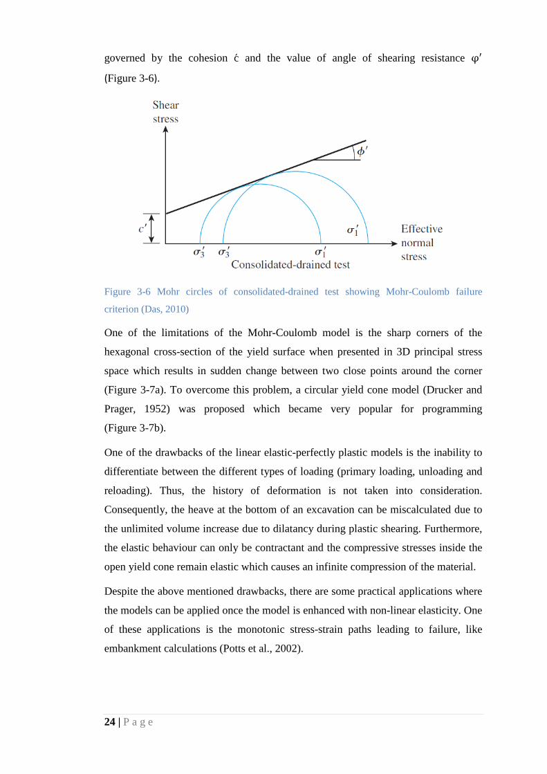
governed by the cohesion c and the value of angle of shearing resistance φ′
(Figure 3-6).
Figure 3-6 Mohr circles of consolidated-drained test showing Mohr-Coulomb failure
criterion (Das, 2010)
One of the limitations of the Mohr-Coulomb model is the sharp corners of the
hexagonal cross-section of the yield surface when presented in 3D principal stress
space which results in sudden change between two close points around the corner
(Figure 3-7a). To overcome this problem, a circular yield cone model (Drucker and
Prager, 1952) was proposed which became very popular for programming
(Figure 3-7b).
One of the drawbacks of the linear elastic-perfectly plastic models is the inability to
differentiate between the different types of loading (primary loading, unloading and
reloading). Thus, the history of deformation is not taken into consideration.
Consequently, the heave at the bottom of an excavation can be miscalculated due to
the unlimited volume increase due to dilatancy during plastic shearing. Furthermore,
the elastic behaviour can only be contractant and the compressive stresses inside the
open yield cone remain elastic which causes an infinite compression of the material.
Despite the above mentioned drawbacks, there are some practical applications where
the models can be applied once the model is enhanced with non-linear elasticity. One
of these applications is the monotonic stress-strain paths leading to failure, like
embankment calculations (Potts et al., 2002).
25 | P a g e
Figure 3-7 Perfectly plastic yield surfaces: (a) Mohr-Coulomb cone, (b) Drucker-Prager cone
(Potts et al., 2002)
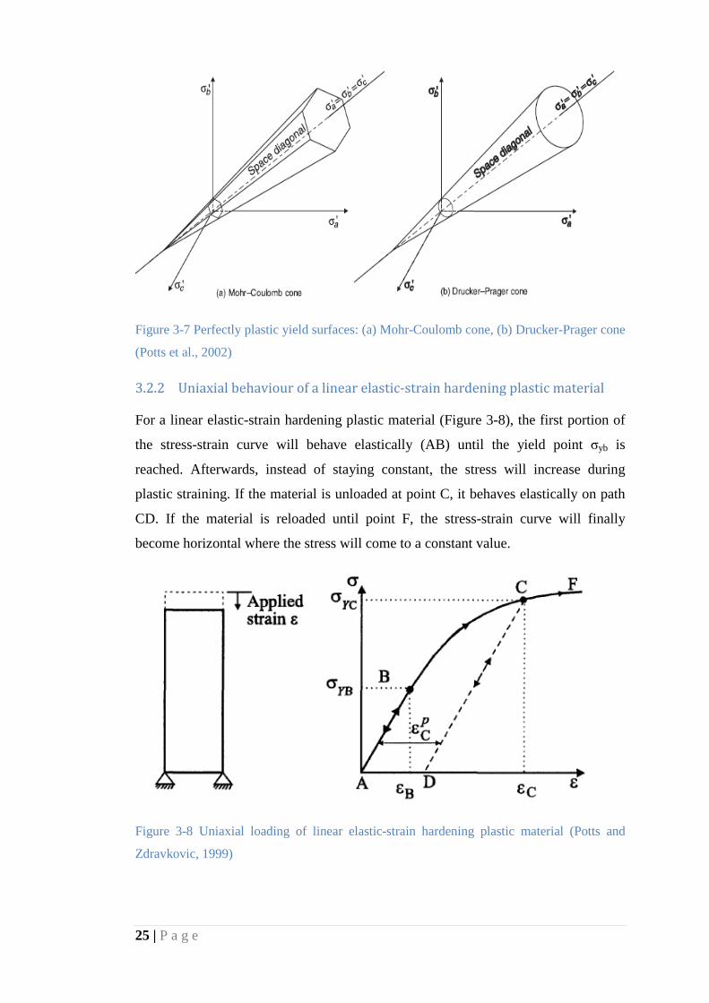
3.2.2 Uniaxial behaviour of a linear elastic-strain hardening plastic material
For a linear elastic-strain hardening plastic material (Figure 3-8), the first portion of
the stress-strain curve will behave elastically (AB) until the yield point σyb is
reached. Afterwards, instead of staying constant, the stress will increase during
plastic straining. If the material is unloaded at point C, it behaves elastically on path
CD. If the material is reloaded until point F, the stress-strain curve will finally
become horizontal where the stress will come to a constant value.
Figure 3-8 Uniaxial loading of linear elastic-strain hardening plastic material (Potts and
Zdravkovic, 1999)

26 | P a g e
One of the early models that allowed for strain hardening was a model with movable
yield cone to replace the fixed one (Drucker, Gibson and Henkel, 1957). This
movable cone allowed for the volumetric plastic strain hardening to take place. In
addition, associated plasticity is assumed where the yield cap was considered the
plastic potential (Figure 3-9). Thus, it became possible to distinguish between
primary loading and unloading-reloading due to the capability of representing
irreversible volumetric and shear plastic strains.
Figure 3-9 Drucker-Gibson-Henkel (1957) cone-cap model (Potts et al., 2002)
3.2.3 Uniaxial behaviour of a linear elastic-strain softening plastic material
For a linear elastic-strain softening plastic material (Figure 3-10), after reaching the
yield point, the stress starts decreasing during plastic straining. The material behaves
in the elastic, unloading and reloading parts similar to the previous plastic materials.
However, during plastic straining, along the path BCF, the yield stress reduces. Such
material is called linear elastic-strain softening material. It is of a particular
consideration due to its brittle nature as, beyond yield point, its capacity to resist
loads falls.
As previously mentioned, after hitting the yield curve in an elastoplastic behaviour, a
combination of elastic and plastic strains starts taking place. In elastoplastic critical
state models, shearing will ultimately bring the soil to a critical state (see
Section 3.2.7). The model is usually described by the triaxial stress variables (p' and
q) and strain variables (εv and εs). The change in size of the yield curve (hardening or
softening) is generally caused by the occurrence of plastic volumetric strains.

27 | P a g e
Figure 3-10 Uniaxial loading of linear elastic-strain softening plastic material (Potts and
Zdravkovic, 1999)
3.2.4 Elastic volumetric strains
The yield curve marks the boundary in which the soil behaves elastically. Stress
increments taking place inside this curve cause only elastic recoverable strains. If the
soil is assumed to behave isotropically elastic, the recoverable elastic strains are
linked only with the change of mean effective stresses p'. The position, shape and
size of the yield curve are results of the loading history of the soil.
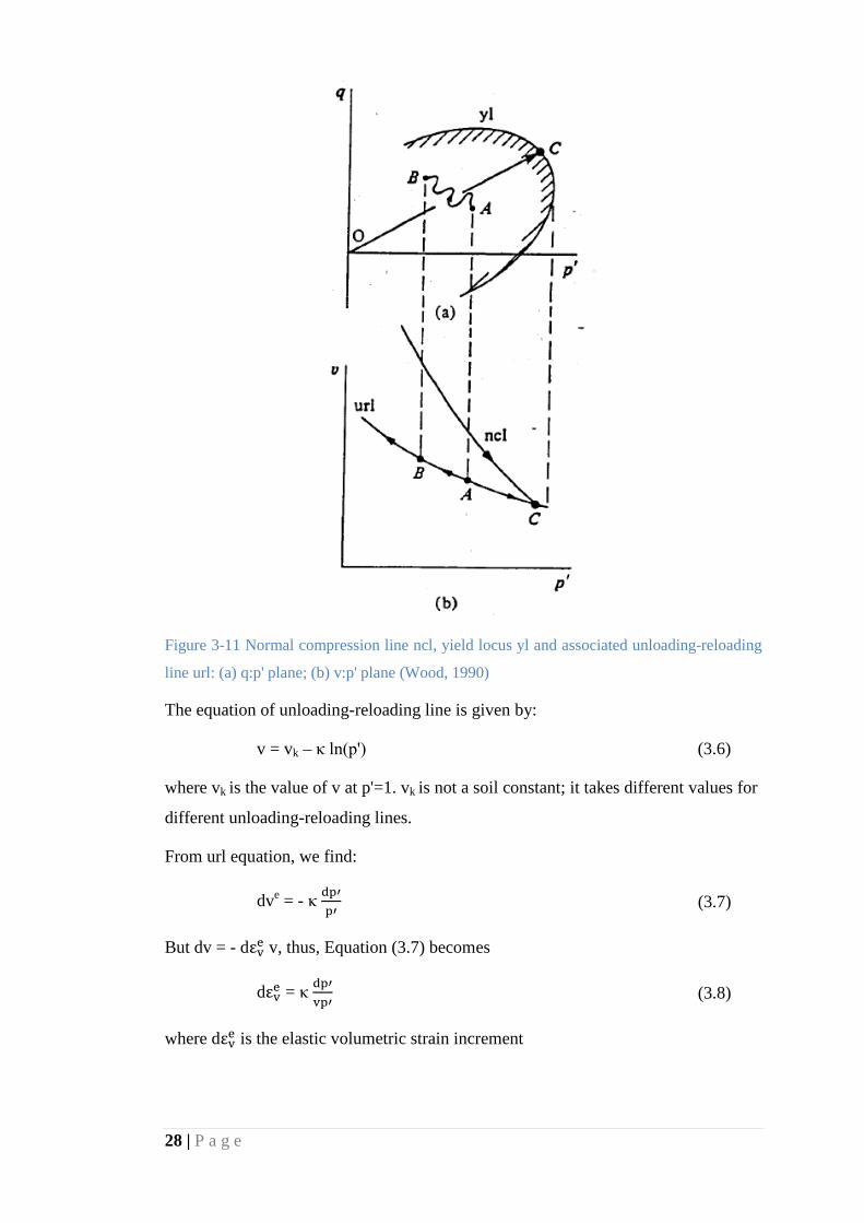
For a soil sample (Figure 3-11) with a yield locus yl in the p':q, a change in p' from
point A to B leads to a change in the volumetric strain. The unloading-reloading line
url from A to B and vice versa is elastic and follows the same path. The normal
compression line ncl is formed by a series of points of p' and v in the normal
compression loading stage. The yield curve has been pushed out to point C which is
associated with the loading history of the soil.
The compression plane (v:p' plane) for ncl and url is usually drawn with a
logarithmic scale for p' which gives better linearity and better extraction of
parameters (Figure 3-12). The equation for normal compression line is given by:
v = N – λ ln(p') (3.5)
where N and λ are soil constants. The value of N is the value of v on the ncl at p’=1
(usually the units of p' are taken as kPa).
28 | P a g e
Figure 3-11 Normal compression line ncl, yield locus yl and associated unloading-reloading
line url: (a) q:p' plane; (b) v:p' plane (Wood, 1990)
The equation of unloading-reloading line is given by:
v = vk – κ ln(p') (3.6)
where vk is the value of v at p'=1. vk is not a soil constant; it takes different values for
different unloading-reloading lines.
From url equation, we find:
dve = - κ dp′p′
(3.7)
But dv = - dεve v, thus, Equation (3.7) becomes
dεve = κ dp′vp′
(3.8)
where dεve is the elastic volumetric strain increment

29 | P a g e
Figure 3-12 Normal compression line and unloading-reloading line in compression plane
(Wood, 1990)
By combining Equations (3.3) and (3.8), the bulk modulus K’ is given by:
K' = vp′κ
(3.9)
Inspecting of Equation 3.9 indicates that, for soils, the bulk modulus K’ is not
constant. Instead, the value of K’ varies with both v and p’ (non-linear elasticity).
3.2.5 Plastic volumetric strains
As the stress state reaches a yield stress (point C on Figure 3-11), plastic strains start
to develop along with the elastic ones. In addition, the size of the yield curve will
start changing while the shape will generally be assumed to stay the same
(Figure 3-4). Assuming a constant shape of the yield curve is a conventional
assumption but not a necessary one, although complexities appear if the curve was
permitted to change in shape (Wood, 1990). Yielding is assumed to be a sudden
phenomenon whereas in reality it is rather gradual.
The total change in the specific volume v is divided into elastic and plastic changes:

30 | P a g e
dv = dve + dvp (3.10)
Using url and ncl equations:
dvp = (λ – κ) dp˳′p˳′
(3.11)
Thus:
dεvp = (λ – κ) dp˳′
vp˳′ (3.12)
where p˳ defines the size of the yield curve (typically taken as the yield stress under
isotropic loading).
It is worth noting that, once the yield curve is reached, for conditions where no
change in volume takes place (undrained loading), elastic and plastic volumetric
strains will still develop where one value will be negative and the other is positive.
3.2.6 Plastic shear strains
The other part of the plastic deformation is the plastic shear strain. Unlike elastic
response, the direction of the plastic strain increment vector is governed by the
combination of stresses at the particular point rather than the route in which yielding
is reached.
As the plastic strains are independent of the stress path and are linked to the
combination of stresses at the yield surface, the direction of the plastic strain
increment vector differs according to which combination of stresses takes place on
the curve.
If the yield surface and the plastic potential surface for any material are identical, the
material is said to follow the postulate of normality where the plastic strain increment
vector is normal to the yield curve (Figure 3-13).
In other words, the soil is said to obey an associated flow rule. The flow rule
specifies the ratio between the plastic shear strain increment and the volumetric shear
strain increment as a function of the current stress state:
dεsp
dεvp = f (p':q) (3.13)

31 | P a g e
In this procedure, it is important that the strain increment parameters are selected in
conjugate pairs with the stress parameters.
Figure 3-13 plastic strain increment vectors normal to a family of plastic potential curves
(Wood, 1990)
In an elastoplastic model, the stress state can either be inside the yield surface (in
which the soil will behave elastically) or on it (in which plastic deformations will
start taking place). The stress state cannot lie outside the yield surface.
One of the most common elastoplastic models is the Cam-clay model which was first
introduced in Cambridge University (Roscoe and Schofield, 1963) and (Schofield
and Wroth, 1968) based on critical state in the same time as the cone-cap model.
Later on, a Modified Cam-clay model MCC was presented (Roscoe and Burland,
1968) in which elliptical yield curve is assumed in the p-q plane (Figure 3-14) along
with an associated flow rule and isotropic hardening and softening.
The actual size of the yield curve is determined according to memory of the soil
history and changes as a function of the plastic volumetric strain.
The model possessed good reputation and popularity due its logic and good
predictive capabilities. However, the model has some drawbacks in which one of
them is the overestimation of peak failure on the dry side of the yield curve. Detailed
description of the MCC model is given in Section 4.1.
32 | P a g e
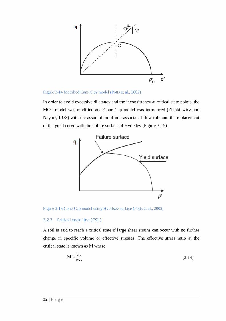
Figure 3-14 Modified Cam-Clay model (Potts et al., 2002)
In order to avoid excessive dilatancy and the inconsistency at critical state points, the
MCC model was modified and Cone-Cap model was introduced (Zienkiewicz and
Naylor, 1973) with the assumption of non-associated flow rule and the replacement
of the yield curve with the failure surface of Hvorslev (Figure 3-15).
Figure 3-15 Cone-Cap model using Hvorlsev surface (Potts et al., 2002)
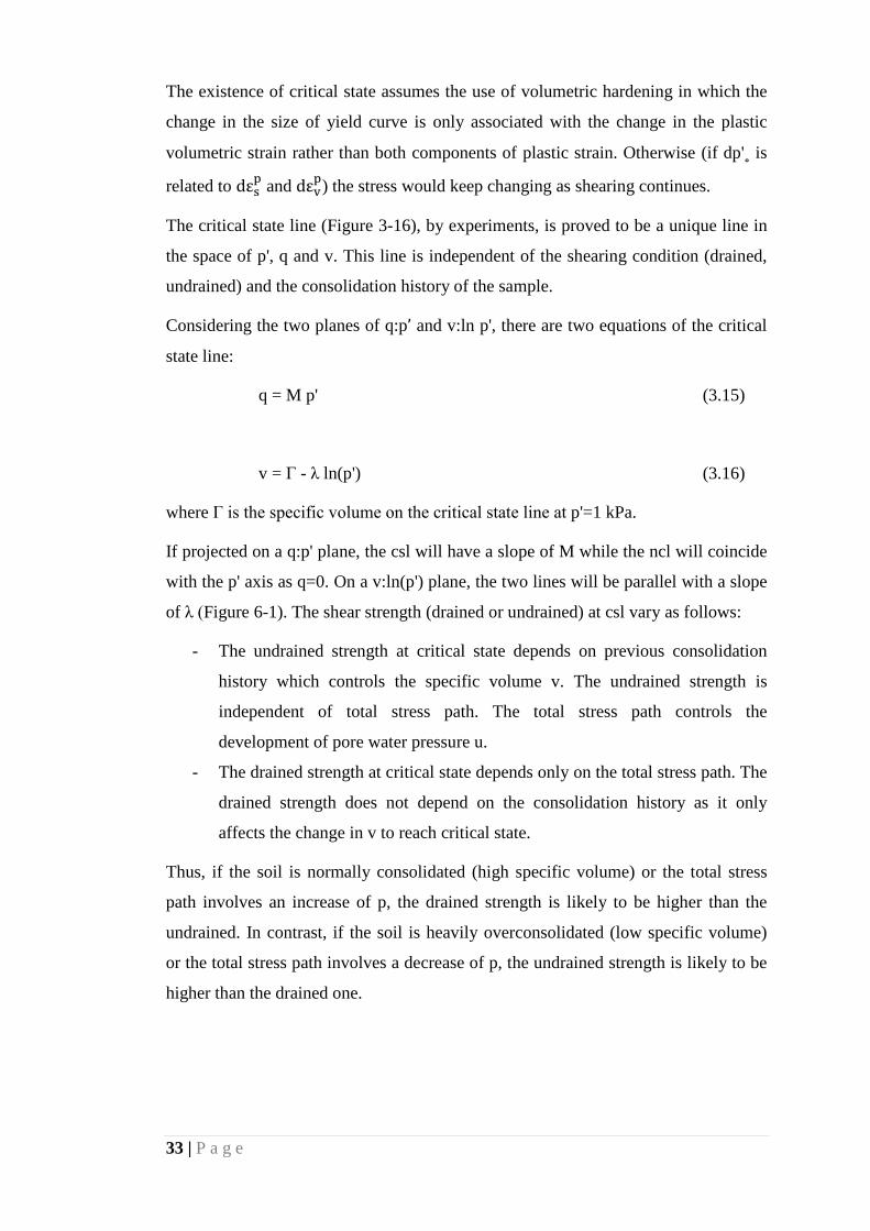
3.2.7 Critical state line (CSL)
A soil is said to reach a critical state if large shear strains can occur with no further
change in specific volume or effective stresses. The effective stress ratio at the
critical state is known as M where
M = qcsp′cs
(3.14)
33 | P a g e
The existence of critical state assumes the use of volumetric hardening in which the
change in the size of yield curve is only associated with the change in the plastic
volumetric strain rather than both components of plastic strain. Otherwise (if dp'˳ is
related to dεsp and dεv
p) the stress would keep changing as shearing continues.
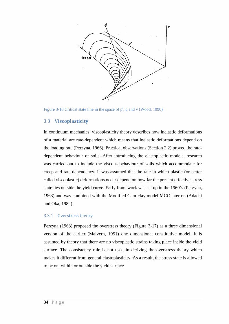
The critical state line (Figure 3-16), by experiments, is proved to be a unique line in
the space of p', q and v. This line is independent of the shearing condition (drained,
undrained) and the consolidation history of the sample.
Considering the two planes of q:p’ and v:ln p', there are two equations of the critical
state line:
q = M p' (3.15)
v = Г - λ ln(p') (3.16)
where Г is the specific volume on the critical state line at p'=1 kPa.
If projected on a q:p' plane, the csl will have a slope of M while the ncl will coincide
with the p' axis as q=0. On a v:ln(p') plane, the two lines will be parallel with a slope
of λ (Figure 6-1). The shear strength (drained or undrained) at csl vary as follows:
- The undrained strength at critical state depends on previous consolidation
history which controls the specific volume v. The undrained strength is
independent of total stress path. The total stress path controls the
development of pore water pressure u.
- The drained strength at critical state depends only on the total stress path. The
drained strength does not depend on the consolidation history as it only
affects the change in v to reach critical state.
Thus, if the soil is normally consolidated (high specific volume) or the total stress
path involves an increase of p, the drained strength is likely to be higher than the
undrained. In contrast, if the soil is heavily overconsolidated (low specific volume)
or the total stress path involves a decrease of p, the undrained strength is likely to be
higher than the drained one.
34 | P a g e
Figure 3-16 Critical state line in the space of p’, q and v (Wood, 1990)
Viscoplasticity 3.3
In continuum mechanics, viscoplasticity theory describes how inelastic deformations
of a material are rate-dependent which means that inelastic deformations depend on
the loading rate (Perzyna, 1966). Practical observations (Section 2.2) proved the rate-
dependent behaviour of soils. After introducing the elastoplastic models, research
was carried out to include the viscous behaviour of soils which accommodate for
creep and rate-dependency. It was assumed that the rate in which plastic (or better
called viscoplastic) deformations occur depend on how far the present effective stress
state lies outside the yield curve. Early framework was set up in the 1960’s (Perzyna,
1963) and was combined with the Modified Cam-clay model MCC later on (Adachi
and Oka, 1982).
3.3.1 Overstress theory
Perzyna (1963) proposed the overstress theory (Figure 3-17) as a three dimensional
version of the earlier (Malvern, 1951) one dimensional constitutive model. It is
assumed by theory that there are no viscoplastic strains taking place inside the yield
surface. The consistency rule is not used in deriving the overstress theory which
makes it different from general elastoplasticity. As a result, the stress state is allowed
to be on, within or outside the yield surface.

35 | P a g e
Figure 3-17 The overstress theory (Perzyna, 1966)
3.3.2 Viscoplastic Soil Models
According to Prevost & Popsecu (1996), “Elastic visco-plastic models appear to be
most promising”. The previously discussed elastoplastic models did not account for
creep as no deformation is predicted by these models when the effective stress is held
constant in the absence of hydrodynamic lag. Several suggestions were proposed in
the late 1960’s about creep rate in clays and its relation to rate of deviatoric stress.
Adachi & Okano (1974) were the first to describe rate-dependant behaviour of soil
media by proposing a general formulation of an elasto-viscoplastic model. Since
then, there have been two main groups of elasto-viscoplastic models: rate formulated
models and creep formulated models. (Prevost and Popsecu, 1996)
• Rate Models
Based on Perzyna’s (1963) viscoplastic experimental results, Adachi & Okano
(1974) proposed their model in which they extended the constitutive equations to
capture the viscous effects of normally consolidated clays. They considered the fully
saturated clay as a mixture of solids (soil skeleton), viscous fluid (absorbed water)
and non-viscous fluid (free water). They proposed two loading functions (yield
surfaces): a static yield surface fs and a dynamic one fd (Figure 3-18a). If the soil is
loaded with a theoretically zero strain rate (very low rate of loading), the stress state
will lie on the static surface. By increasing the loading rate, the stress state will lie on
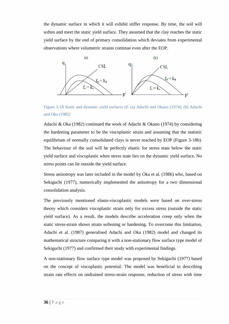
36 | P a g e
the dynamic surface in which it will exhibit stiffer response. By time, the soil will
soften and meet the static yield surface. They assumed that the clay reaches the static
yield surface by the end of primary consolidation which deviates from experimental
observations where volumetric strains continue even after the EOP.
Figure 3-18 Static and dynamic yield surfaces of: (a) Adachi and Okano (1974); (b) Adachi
and Oka (1982)
Adachi & Oka (1982) continued the work of Adachi & Okano (1974) by considering
the hardening parameter to be the viscoplastic strain and assuming that the statistic
equilibrium of normally consolidated clays is never reached by EOP (Figure 3-18b).
The behaviour of the soil will be perfectly elastic for stress state below the static
yield surface and viscoplastic when stress state lies on the dynamic yield surface. No
stress points can lie outside the yield surface.
Stress anisotropy was later included in the model by Oka et al. (1986) who, based on
Sekiguchi (1977), numerically implemented the anisotropy for a two dimensional
consolidation analysis.
The previously mentioned elasto-viscoplastic models were based on over-stress
theory which considers viscoplastic strain only for excess stress (outside the static
yield surface). As a result, the models describe acceleration creep only when the
static stress-strain shows strain softening or hardening. To overcome this limitation,
Adachi et al. (1987) generalised Adachi and Oka (1982) model and changed its
mathematical structure comparing it with a non-stationary flow surface type model of
Sekiguchi (1977) and confirmed their study with experimental findings.
A non-stationary flow surface type model was proposed by Sekiguchi (1977) based
on the concept of viscoplastic potential. The model was beneficial in describing
strain rate effects on undrained stress-strain response, reduction of stress with time
37 | P a g e
(stress relaxation) and the characteristics of creep rapture (the summit in the
deformation process of creep).
Several other elasto-viscoplastic models were developed based on Perzyna’s (1963,
1966) theory of viscoplasticity. Liang & Ma (1992) developed a unified elasto-
viscoplastic model having the limit surface and the conjugate static yield surface as
the basic framework. The preconsolidation pressure (affected by the aging effect)
was chosen to predict time and rate effects. Another elasto-viscoplastic model was
proposed by Rowe & Hinchberger (1998) in which they modified Adachi & Oka
(1982) model with an elliptical cap.
• Creep Models
The base of these models was Bjerrum’s (1967) concept of delayed compression and,
to some extent, the MCC model. Bjerrum (1967) divided soil deformations into
“immediate” and “delayed” compression. Based on this concept, Borja &
Kavazanjian (1985) used the MCC model to describe the time-dependant
elastoplastic strains of clays. Theory of plasticity was used to describe the time-
independent stress-strain behaviour using the elliptical yield surface of the MCC
model. Two parts were used (elastic and plastic) to describe the time-dependant
behaviour of the model using associated flow rule and consistency requirement on
the yield surface. The model requires 13 parameters for a proper description of soil
behaviour.
A double yield surface model was proposed by Hsieh et al. (1990) as a development
of Borja & Kavazanjian (1985) model. The model takes into consideration plastic
shear distortion which takes place without volume change below the state boundary
surface. In addition, the model provides more accurate predictions than the MCC
model especially at low strain levels. The model stayed complex in terms of required
parameters as it needed 13 parameters if creep is to be taken into considerations.
Yin & Graham (1989) proposed a one dimensional model for stepped loading using
the “equivalent time” concept during time dependant straining. Next, the model was
developed into general constitutive equation for continuous loading. The model
assumed unloading to be independent of time. However, the model underestimated
the effect of time and loading rate on the undrained shear strength. Yin & Zhu (1999)
38 | P a g e
developed their previous model to simulate creep acceleration when the deviatoric
stress approaches shear strength envelope. Furthermore, the model takes unloading-
reloading and relaxation into account in addition to providing realistic simulation of
effect of shearing rate. They used the MCC model and Perzyna’s (1966) theory of
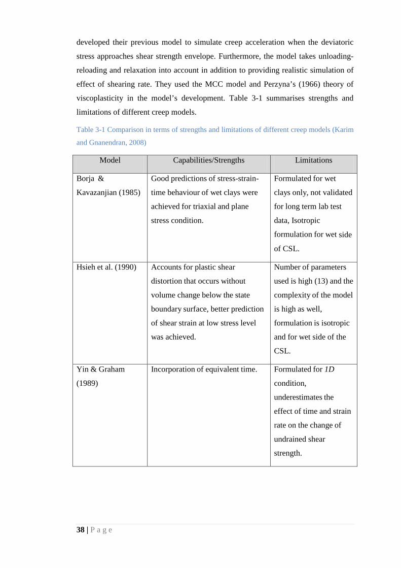
viscoplasticity in the model’s development. Table 3-1 summarises strengths and
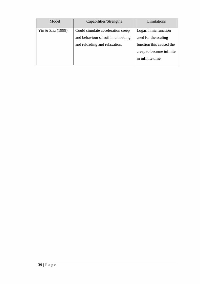
limitations of different creep models.
Table 3-1 Comparison in terms of strengths and limitations of different creep models (Karim
and Gnanendran, 2008)
Model Capabilities/Strengths Limitations
Borja &
Kavazanjian (1985)
Good predictions of stress-strain-
time behaviour of wet clays were
achieved for triaxial and plane
stress condition.
Formulated for wet
clays only, not validated
for long term lab test
data, Isotropic
formulation for wet side
of CSL.
Hsieh et al. (1990) Accounts for plastic shear
distortion that occurs without
volume change below the state
boundary surface, better prediction
of shear strain at low stress level
was achieved.
Number of parameters
used is high (13) and the
complexity of the model
is high as well,
formulation is isotropic
and for wet side of the
CSL.
Yin & Graham
(1989)
Incorporation of equivalent time.
Formulated for 1D
condition,
underestimates the
effect of time and strain
rate on the change of
undrained shear
strength.
39 | P a g e
Model Capabilities/Strengths Limitations
Yin & Zhu (1999)
Could simulate acceleration creep
and behaviour of soil in unloading
and reloading and relaxation.
Logarithmic function
used for the scaling
function this caused the
creep to become infinite
in infinite time.
40 | P a g e
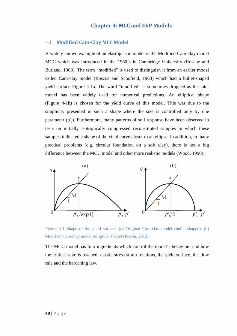
Chapter 4: MCC and EVP Models 4
Modified Cam-Clay MCC Model 4.1
A widely known example of an elastoplastic model is the Modified Cam-clay model
MCC which was introduced in the 1960’s in Cambridge University (Roscoe and
Burland, 1968). The term “modified” is used to distinguish it from an earlier model
called Cam-clay model (Roscoe and Schofield, 1963) which had a bullet-shaped
yield surface Figure 4-1a. The word “modified” is sometimes dropped as the later
model has been widely used for numerical predictions. An elliptical shape
(Figure 4-1b) is chosen for the yield curve of this model. This was due to the
simplicity presented in such a shape where the size is controlled only by one
parameter (p'˳). Furthermore, many patterns of soil response have been observed in
tests on initially isotropically compressed reconstituted samples in which these
samples indicated a shape of the yield curve closer to an ellipse. In addition, in many
practical problems (e.g. circular foundation on a soft clay), there is not a big
difference between the MCC model and other more realistic models (Wood, 1990).
Figure 4-1 Shape of the yield surface: (a) Original Cam-clay model (bullet-shaped). (b)
Modified Cam-clay model (elliptical shape) (Puzrin, 2012)
The MCC model has four ingredients which control the model’s behaviour and how
the critical state is reached: elastic stress strain relations, the yield surface, the flow
rule and the hardening law.

41 | P a g e
4.1.1 Elastic stress-strain relations
For stresses combination inside the yield curve, elastic strains take place and the
elastic volumetric strain is calculated according to the expression:
dεve = κ dp′v p′
(4.1)
For elastic unloading-reloading, Equation (4.1) implies a linear relationship in
v:ln(p') plane between specific volume and logarithm of p'.
The elastic shear strains are associated with the change in the deviatoric stress q
according to the following equation:
dεse = dq3 G′
(4.2)
where G' is the shear modulus (Equation 3.2).
4.1.2 Yield surface
The yield surface (Figure 4-2) takes the shape of an ellipse where its size is only
controlled by the value of p'˳. The ellipse can be described using the following
equation:
p′p′˳
= M2
M2+ η2 (4.3)
where η = q/p’ and M is the aspect ratio of the yield curve and the slope of the critical
state line in the q': p' plot. This equation describes a set of ellipses all passing through
the origin with the same shape (controlled by M) with the size controlled by the
change in p˳. Equation 4.3 can be rewritten as:
q2 = M2 p′(p′˳ − p′) (4.4)
4.1.3 Flow rule
Since an associated flow rule is assumed for this model, the plastic strain increment
vector is normal to the yield surface. Thus, the plastic potential has the same shape
and equation as the yield curve.

42 | P a g e
Figure 4-2 Yield curve of the Modified Cam-Clay (MCC) model
Differentiating the plastic potential equation with respect to p' and rearranging it:
dqdp′
= M2 p′˳ − 2p′
2q (4.5)
Since associated flow rule applies, then
dεv
p
dεvp =
−1
( dqdp′)
(4.6)
Thus, when the plastic deformations are occurring, from equations (4.5) and (4.6):
dεs
p
dεvp =
2ηM2 − η2
(4.7)
4.1.4 Hardening Law
As discussed earlier, the change in the size of the yield curve is linked to the
development of volumetric plastic strains and is independent of the plastic shear
strain. Thus, from ncl equation, we find:
-300
-200
-100
0
100
200
300
0 50 100 150 200 250 300 350
q
p'
Yield curve
p'˳
M p'˳
CSL M
1
43 | P a g e
dεvp = (λ – κ) dp′˳
v p′˳ (4.8)
Once dεvp is calculated, the plastic shear strains can be found using the flow rule
(Equation 4.7).
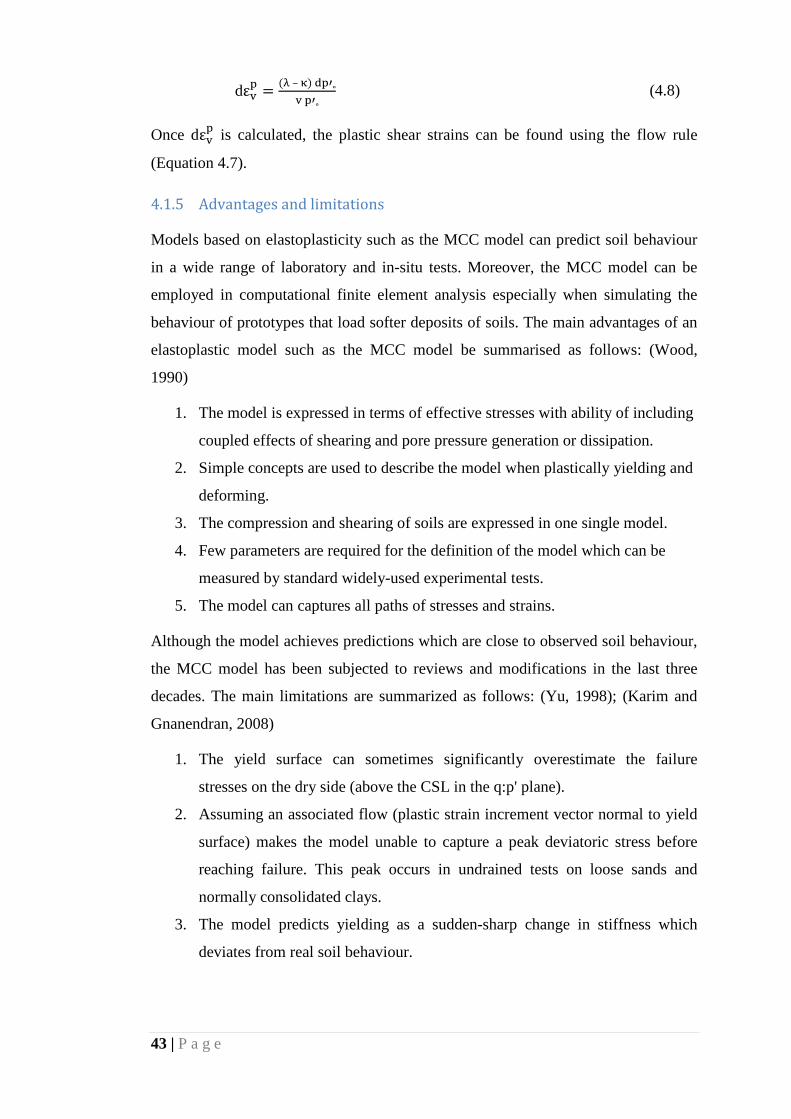
4.1.5 Advantages and limitations
Models based on elastoplasticity such as the MCC model can predict soil behaviour
in a wide range of laboratory and in-situ tests. Moreover, the MCC model can be
employed in computational finite element analysis especially when simulating the
behaviour of prototypes that load softer deposits of soils. The main advantages of an
elastoplastic model such as the MCC model be summarised as follows: (Wood,
1990)
1. The model is expressed in terms of effective stresses with ability of including
coupled effects of shearing and pore pressure generation or dissipation.
2. Simple concepts are used to describe the model when plastically yielding and
deforming.
3. The compression and shearing of soils are expressed in one single model.
4. Few parameters are required for the definition of the model which can be
measured by standard widely-used experimental tests.
5. The model can captures all paths of stresses and strains.
Although the model achieves predictions which are close to observed soil behaviour,
the MCC model has been subjected to reviews and modifications in the last three
decades. The main limitations are summarized as follows: (Yu, 1998); (Karim and
Gnanendran, 2008)
1. The yield surface can sometimes significantly overestimate the failure
stresses on the dry side (above the CSL in the q:p' plane).
2. Assuming an associated flow (plastic strain increment vector normal to yield
surface) makes the model unable to capture a peak deviatoric stress before
reaching failure. This peak occurs in undrained tests on loose sands and
normally consolidated clays.
3. The model predicts yielding as a sudden-sharp change in stiffness which
deviates from real soil behaviour.

44 | P a g e
4. The model is not efficient when modelling granular materials as it cannot
capture the softening and dilatancy of dense sand as well as the undrained
response of very loose sands.
5. Due to isotropy in its formulation, the model cannot properly explain the k0
compression behaviour of soil.
Elasto-viscoplastic (EVP) Model 4.2
An EVP model proposed by Wheeler (2011) is used in this study based on
hypothesis B of creep and compared to the MCC model by the mean of conventional
triaxial compression tests. Unlike overstress models, this model assumes viscoplastic
strains to be continuously taking place, even inside the yield surface. This
assumption came from practical observations of overconsolidated soils where
significant creep strains are present in the elastic region. The model introduces the
effect of creep and rate effect in soft soil and disregard anisotropy and other effects
in order to keep the model comparable to the MCC model. The model has four
ingredients which control the model’s behaviour and how the critical state is reached:
elastic stress strain relations, the viscoplastic curve, the flow rule and the viscoplastic
relations.
4.2.1 Elastic stress-strain relations
The equations for the elastic parts of the strains are the same as the ones in the MCC
model.
4.2.2 Viscoplastic Curve
In order to ensure comparability with the MCC model, the viscoplastic curve has the
same shape and equation as the MCC. However, it behaves differently. The curve
cannot be called a “yield curve” as there are inelastic strains developing inside in it.
The size of the viscoplastic curve is controlled by the viscoplastic volumetric strain
increment. The stress point can either be inside, on or outside the viscoplastic curve
where the farther from the curve the higher the rate of viscoplastic volumetric strain
increment dεvvp/dt will be (Figure 4-3). The viscoplastic curve is defined by:
q2 = M2 p′(p′˳ − p′) (4.9)
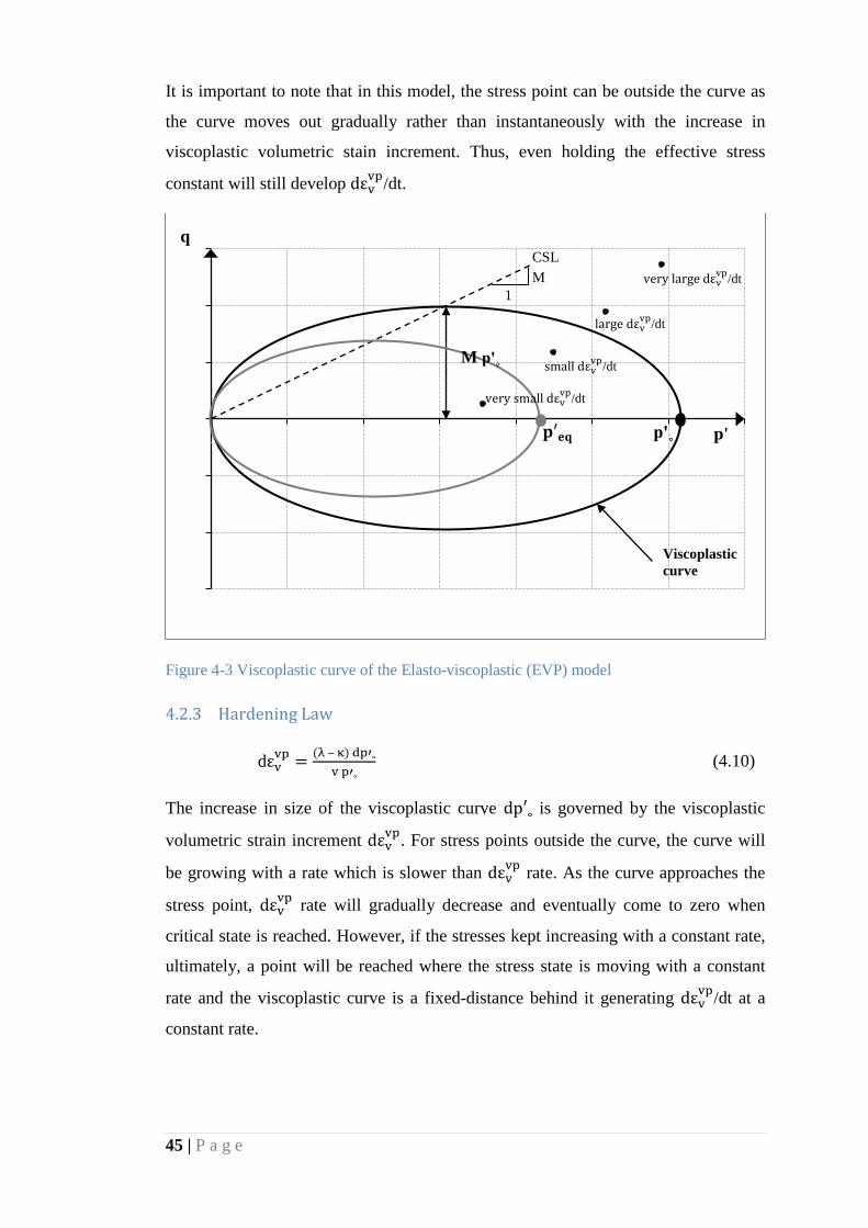
45 | P a g e
It is important to note that in this model, the stress point can be outside the curve as
the curve moves out gradually rather than instantaneously with the increase in
viscoplastic volumetric stain increment. Thus, even holding the effective stress
constant will still develop dεvvp/dt.
Figure 4-3 Viscoplastic curve of the Elasto-viscoplastic (EVP) model
4.2.3 Hardening Law
dεvvp = (λ – κ) dp′˳
v p′˳ (4.10)
The increase in size of the viscoplastic curve dp′˳ is governed by the viscoplastic
volumetric strain increment dεvvp. For stress points outside the curve, the curve will
be growing with a rate which is slower than dεvvp rate. As the curve approaches the
stress point, dεvvp rate will gradually decrease and eventually come to zero when
critical state is reached. However, if the stresses kept increasing with a constant rate,
ultimately, a point will be reached where the stress state is moving with a constant
rate and the viscoplastic curve is a fixed-distance behind it generating dεvvp/dt at a
constant rate.
-300
-200
-100
0
100
200
300
0 50 100 150 200 250 300 350
q
p'
Viscoplastic curve
p'˳
M p'˳
CSL M
1
𝐩′𝐞𝐞
very small dεvvp/dt
small dεvvp/dt
large dεvvp/dt
very large dεvvp/dt

46 | P a g e
4.2.4 Viscoplastic relation
Wheeler (2011) proposed the following relation for the calculation of the rate of
change of viscoplastic volumetric strain increment dεvvp/dt:
dεvvp
dt = (M
2−η2
M2 ) µv T
(p′eqp′˳
)λ – κµ (4.11)
where μ is the slope of the straight portion of the curve in the v:ln(t) plane
(Figure 6-2). μ can be considered as another representation of creep index (cα) where
μ = cα/ln(10). p'eq is the equivalent mean effective stress of a given stress point that
forms a curve with the same aspect ratio of the viscoplastic curve (Figure 4-3).
T is a time constant related to the reference time that is used to define the current
position of viscoplastic curve (p′˳). The current position of curve reflects the history
of the soil and what it has been through during its historical age. For example, if two
simulations are to be done for the same soil with all parameters being the same
including the value of p′˳ (the initial position of the viscoplastic curve) but with
different T values, there would be a slight difference in results between the two
simulations. On the other hand, if a proper value of the starting p′˳ is set for each
simulation, using different time constant will result in the exact values for each
simulation.
The rate of dεvvp is dependent on the position of current stress state in comparison to
the viscoplastic curve which is represented by the term (p′eq/p′˳). It can be seen
from Equation 4.12 that once the stress point is outside the viscoplastic curve, the
ratio between p′eq and p′˳ will be greater than one. As this happens, high viscoplastic
strain rate will be developing as this value is raised to a power {(λ – κ)/μ} which is
greater than one.
Another important aspect of this model in comparison with other elasto-viscoplastic
models (e.g. soft soil creep model) is the term (M2−η2
M2 ) in Equation 4.12. This term
relates the stress state with the critical state which is reached once M = η resulting
zero viscoplastic volumetric strain rate and thus no change in size of the viscoplastic
curve.

47 | P a g e
4.2.5 Flow rule
An associated flow rule is assumed for this model (which applies for most of
observed earth materials).
dεv
p
dεvp =
2ηM2 − η2
(4.12)
Thus, from Equations 4.12 and 4.13, the rate of change in viscoplastic shear strain
increment can be found as follows:
dεsvp
dt = (2η
M2) µv T
(p′eqp′˳
)λ – κµ (4.13)
4.2.6 EVP Advantages over MCC
The main advantages for the EVP model under consideration can be summarised as
follows:
1. The model captures creep effect even when the stress is held constant.
2. The effect of geological aging of the soil is presented in the model.
3. The model account for the rate of shearing in which different rates give
different results as will be discussed in Chapter 6.
4. Unlike the MCC model, a gradual change in yielding is simulated by the
model (stress-controlled) which is closer to real soil behaviour. This change
is not “transitional” as viscoplastic strains have been taking place since the
beginning of loading.
However, the full capabilities of the proposed EVP model need to be further
investigated with a proper direct quantitative comparison with real soil experiments.
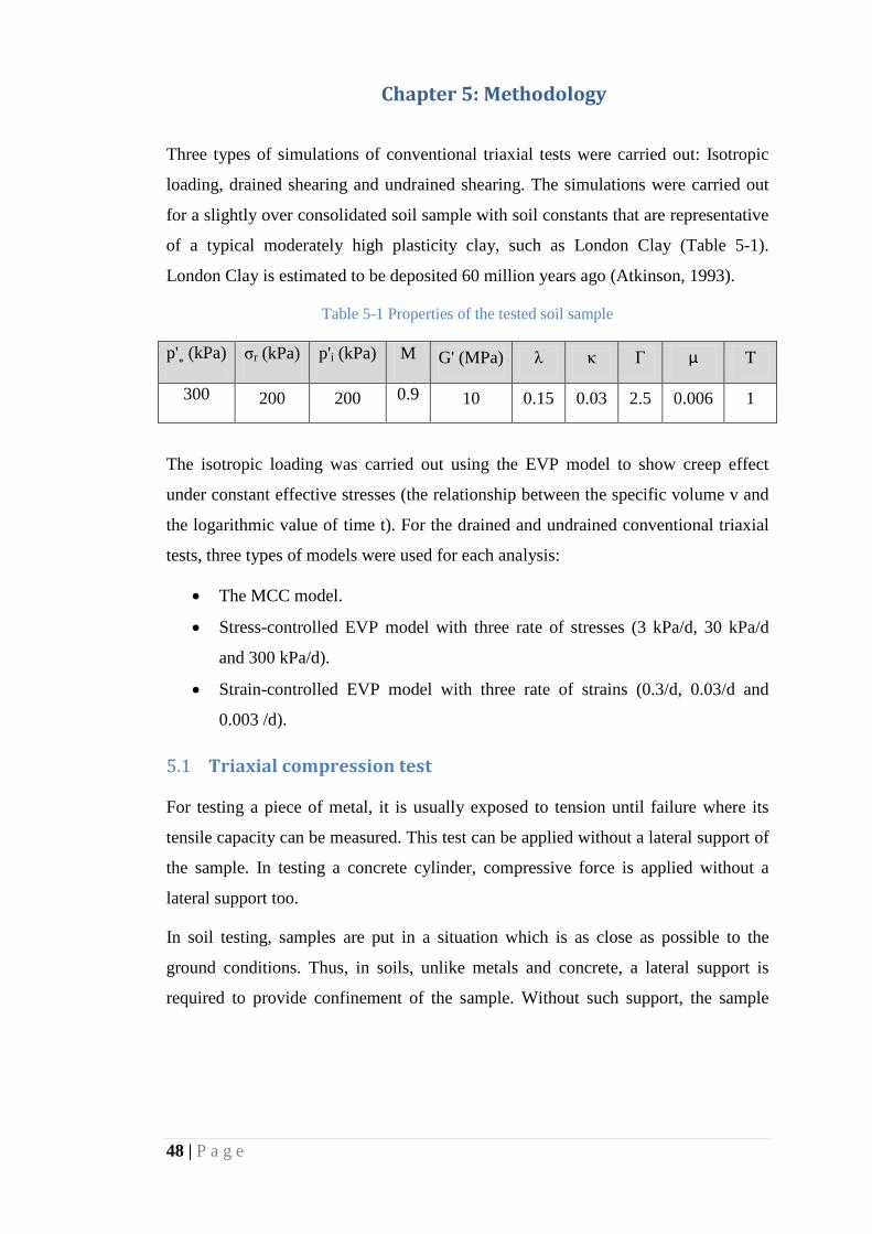
48 | P a g e
Chapter 5: Methodology 5
Three types of simulations of conventional triaxial tests were carried out: Isotropic
loading, drained shearing and undrained shearing. The simulations were carried out
for a slightly over consolidated soil sample with soil constants that are representative
of a typical moderately high plasticity clay, such as London Clay (Table 5-1).
London Clay is estimated to be deposited 60 million years ago (Atkinson, 1993).
Table 5-1 Properties of the tested soil sample
p'˳ (kPa) σr (kPa) p'i (kPa) M G' (MPa) λ κ Г μ T
300 200 200 0.9 10 0.15 0.03 2.5 0.006 1
The isotropic loading was carried out using the EVP model to show creep effect
under constant effective stresses (the relationship between the specific volume v and
the logarithmic value of time t). For the drained and undrained conventional triaxial
tests, three types of models were used for each analysis:
• The MCC model.
• Stress-controlled EVP model with three rate of stresses (3 kPa/d, 30 kPa/d
and 300 kPa/d).
• Strain-controlled EVP model with three rate of strains (0.3/d, 0.03/d and
0.003 /d).
Triaxial compression test 5.1
For testing a piece of metal, it is usually exposed to tension until failure where its
tensile capacity can be measured. This test can be applied without a lateral support of
the sample. In testing a concrete cylinder, compressive force is applied without a
lateral support too.
In soil testing, samples are put in a situation which is as close as possible to the
ground conditions. Thus, in soils, unlike metals and concrete, a lateral support is
required to provide confinement of the sample. Without such support, the sample
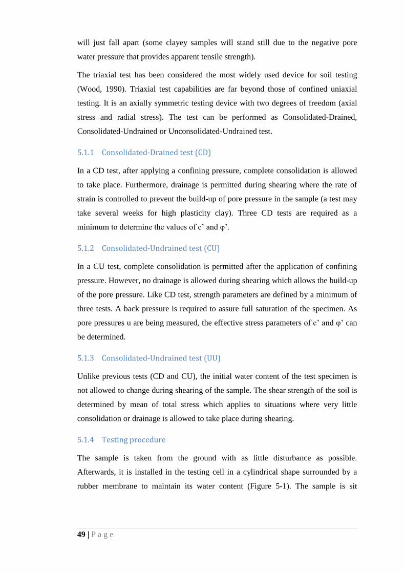
49 | P a g e
will just fall apart (some clayey samples will stand still due to the negative pore
water pressure that provides apparent tensile strength).
The triaxial test has been considered the most widely used device for soil testing
(Wood, 1990). Triaxial test capabilities are far beyond those of confined uniaxial
testing. It is an axially symmetric testing device with two degrees of freedom (axial
stress and radial stress). The test can be performed as Consolidated-Drained,
Consolidated-Undrained or Unconsolidated-Undrained test.
5.1.1 Consolidated-Drained test (CD)
In a CD test, after applying a confining pressure, complete consolidation is allowed
to take place. Furthermore, drainage is permitted during shearing where the rate of
strain is controlled to prevent the build-up of pore pressure in the sample (a test may
take several weeks for high plasticity clay). Three CD tests are required as a
minimum to determine the values of c’ and φ’.
5.1.2 Consolidated-Undrained test (CU)
In a CU test, complete consolidation is permitted after the application of confining
pressure. However, no drainage is allowed during shearing which allows the build-up
of the pore pressure. Like CD test, strength parameters are defined by a minimum of
three tests. A back pressure is required to assure full saturation of the specimen. As
pore pressures u are being measured, the effective stress parameters of c’ and φ’ can
be determined.
5.1.3 Consolidated-Undrained test (UU)
Unlike previous tests (CD and CU), the initial water content of the test specimen is
not allowed to change during shearing of the sample. The shear strength of the soil is
determined by mean of total stress which applies to situations where very little
consolidation or drainage is allowed to take place during shearing.
5.1.4 Testing procedure
The sample is taken from the ground with as little disturbance as possible.
Afterwards, it is installed in the testing cell in a cylindrical shape surrounded by a
rubber membrane to maintain its water content (Figure 5-1). The sample is sit
50 | P a g e
between a firm base and a rigid top which is loaded axially. The top and bottom
boundaries of the cell are porous to allow for drainage if required.
Figure 5-1 Schematic diagram of triaxial test (Wood, 1990)
The triaxial test measures the values of the cell pressure σr (the lateral support), the
pressure in the cell fluid, and the change in the length of sample dl. For drained
shearing, the change in the volume of the sample dV is measured as the volume of the
water dissipated assuming no soil particle compressibility. On the other hand, for
undrained shearing, the test measures the value of the pore water pressure developing
during the test.
As the cell pressure is held constant in a conventional triaxial test, the deviatoric
stress (q = σa-σr) is calculated by dividing the applied force F over the cross sectional
area of the sample A. The stress variables resulting from triaxial test which are under
consideration are mainly the measured ones (cell pressure σr and deviatoric stress q).
The deviatoric stress q and the mean effective stress p' are defined by:
p' = σ′a+ 2 σ′r3
(5.1)

51 | P a g e
q = σ′a − σ′r (5.2)
Where q is the same whether expressed in terms of effective or total stresses (u value
will be eliminated).
By relating stress to strains using work input increments, the two components of the
strain vector can be defined by:
dεv = dεa + 2 dεr (5.3)
dεs = 2(dεa− dεr)3
(5.4)
The mean total stress p is related to q by the following equation:
p = σr + q3 (5.5)
Thus, for a conventional triaxial test (σr = constant), q:p line changes with a slope of
3:1.
5.1.5 Data presentation
In conventional triaxial test with constant cell pressure, data is usually presented by
plots (Figure 5-2) of the variation of deviatoric stress with axial strain, volumetric
strain with axial strain (drained condition) and the variation of pore pressure with the
axial strain (undrained condition). In addition, plots of effective stress plane q:p'
(Figure 5-3) are presented to show the paths of drained (path AB) and undrained
(path AC) tests as well as plots of specific volume v against mean effective stress p'
(compression plane).
Isotropic Loading 5.2
In this analysis, in order to show the capability of the EVP model to account for
creep at a constant stress, Isotropic load was applied (σa = σr) generating a mean
effective stress p' of 400 kPa from a starting value of 200 kPa in one step. The new
value of p' became greater than p'˳ (400 > 300) which in-turn generated a significant
value of dεvvp/dt. As a result, the viscoplastic curve massively increased in size
because the new stress state is outside the curve.
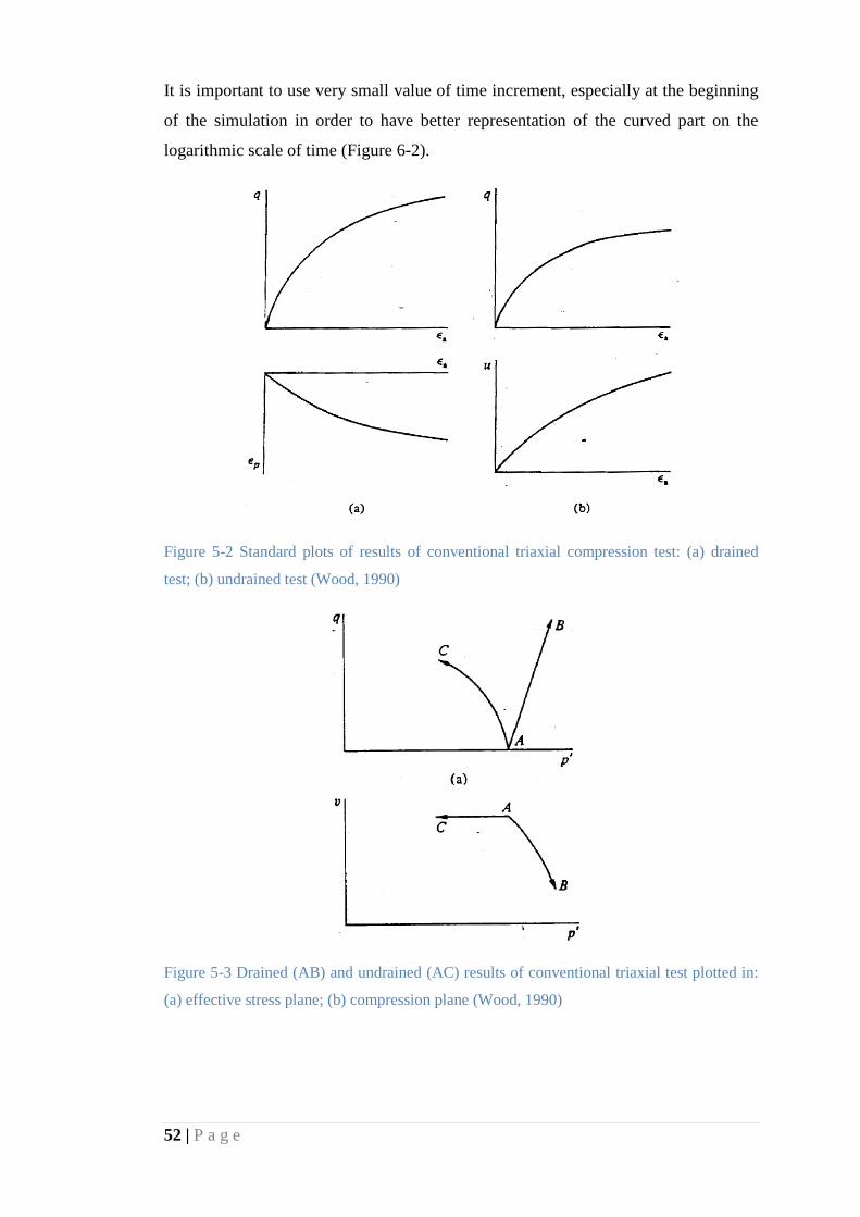
52 | P a g e
It is important to use very small value of time increment, especially at the beginning
of the simulation in order to have better representation of the curved part on the
logarithmic scale of time (Figure 6-2).
Figure 5-2 Standard plots of results of conventional triaxial compression test: (a) drained
test; (b) undrained test (Wood, 1990)
Figure 5-3 Drained (AB) and undrained (AC) results of conventional triaxial test plotted in:
(a) effective stress plane; (b) compression plane (Wood, 1990)

53 | P a g e
5.2.1 Calculation method
The simulation was done by exerting a change in the mean effective stress from 200
kPa to 400 kPa within a time interval of zero. This change in p' resulted in an elastic
change in the specific volume Δve. No further change in Δve was observed as p' was
held constant. Next, the value of dεvvp/dt was calculated using Equation 4.12. The
first few values of dεvvc/dt were significantly large due to the sudden change in the
stress state and exerting a new value of p' greater than p'˳. The value of dεvvp was
then calculated by multiplying its rate of change by the time interval. Next, dvvp was
calculated by multiplying the previous specific volume v by dεvvp. The incremental
change in volume dv is the sum of Δve and dvvp. The new value of v was found by
adding its previous value to the calculated value of dv (the value of v was
decreasing). Afterwards the change of p'˳ (dp'˳) was calculated by Equation 4.11 in
which a new value of p'˳ was then found by adding its previous value to dp'˳. In this
type of loading, p'eq = p' as there is not deviatoric stress generated (σa = σr). Likewise,
there are no shear strains εs developing due to the absence of q. Refer to Appendix A
for detailed tables of calculations.
Drained Shearing 5.3
The soil sample was simulated in a conventional triaxial test under drained shearing.
The test was carried out in an adequate time to assure drained condition. The two
models used are MCC and EVP where the following relationships were investigated:
• The relationship between the mean effective stress p' and the deviatoric stress
q: how p' interacts with q and how this goes with the yield curve and the
elasto-viscoplastic curve.
• The relationship between specific volume v and the mean effective stress p'.
• The relationship between the deviatoric stress q and the shear strain εs.
• The relationship between the volumetric strain εv and the shear strain εs.
It is worth mentioning that the 3-D critical state is expressed by the relationship
between p', q and v. However, this 3-D relationship can be expressed by the two 2-D
graphs of p' vs. q and v vs. ln(p').
54 | P a g e
5.3.1 Calculation method
• Modified Cam Clay model (MCC):
The simulation was carried out by increasing the deviatoric stress q which in-turn
increased the mean effective stress p' by 1:3 (drained condition). Next, the equivalent
mean effective stress p'eq was calculated using Equation 4.4 of the yield curve. The
value of p'˳ was fixed to 300 kPa which is the starting value until p'eq became greater
than 300 kPa. When this happened, the value of p'˳ used in the simulation became as
each new value of p'eq. This means that we have reached the yield point and the yield
curve started increasing in size which resulted in plastic strains beside elastic ones.
The elastic volumetric strain increment dεve was calculated using Equation 4.1.
Afterwards, the elastic shear strain increment dεse was calculated using Equation 4.2.
The plastic volumetric strain increment dεvp was then calculated using the hardening
law (Equation 4.8). Using the flow rule (Equation 4.5), the plastic shear strain
increment dεsp was calculated. After summing the elastic and plastic parts of each
strain type, the total shear strain and volumetric strain were calculated. The change in
the specific volume dv was found by multiplying the initial value of v by the
volumetric strain increment dεv. The final value of v was the sum of vi and dv. Refer
to Appendix B for detailed tables of calculations.
• Elasto-viscoplastic model (EVP) – stress controlled:
For the stress controlled test, a deviatoric stress increment was applied with different
rates (3 kPa/d, 30 kPa/d and 300 kPa/d). Choosing a suitable time increment size was
essential in this model as the calculated εvvc/dt varies significantly with the stress
state. Thus, a relatively small time increment was required, especially for high rate of
shearing.
Starting with the initial value of p'=200 kPa and q=0, a deviatoric stress increment
was applied with the specific rate chosen. The value of p' increased with a rate of 1:3
(drained condition) as q increases. Unlike the MCC model, the value of p'eq is
independent from the value of p'˳. This is because in the EVP model, the stress point
can be outside the viscoplastic curve (there are no restrictions on being inside, on or
outside the curve). The value of p'eq was calculated using the equation of the

55 | P a g e
viscoplastic curve (Equation 4.9). The elastic parts of the strains were then calculated
using the same equations mentioned in the MCC model. The rate of change of the
viscoplastic volumetric strain increment dεvvp/dt was calculated using Equation 4.11.
The viscoplastic volumetric strain increment dεvvp was then calculated by multiplying
its rate of change by the time interval. For the shear strain, the rate of change of the
viscoplastic shear strain increment dεsvp/dt was calculated using Equation 4.13. The
viscoplastic shear strain increment dεsvp was then calculated by multiplying its rate of
change by the time interval. The total elastic strain and the total shear strain were
then found by adding together the two parts of the strains (the elastic part and the
viscoplastic part). The new specific volume was then calculated as mentioned earlier
in the MCC model. The viscoplastic curve increased in size as the value of p'˳
increases in a response to a change in the viscoplastic volumetric strain. This
incremental increase dp'˳ was calculated using the hardening law (Equation 4.11).
Refer to Appendix B for detailed tables of calculations.
• Elasto-viscoplastic model (EVP) – strain controlled:
For the strain controlled test, a shear strain increment was applied with different rates
(0.3 /d, 0.03 /d and 0.003 /d). Choosing a suitable time increment size was essential
in this model as the calculated εvvc/dt varies significantly with the state of stresses.
Thus, a relatively small time increment was required, especially for high shear strain
rate. Otherwise, negative values of dq will result due to the non-linear change in
εvvc/dt for relatively large intervals of time.
Starting with a specific rate of straining, the total shear increment dεs was an input
in the simulation. Next, the rate of change of the viscoplastic shear strain increment
dεsvp/dt, dεs
vp and dεse were calculated as mentioned in the preceding simulation.
Unlike stress controlled test, the deviatoric strain increment dq was calculated as a
response to the elastic shear strain increment dεse using Equation 4.2. The values of
p', dεve, dεvvp/dt, dεv
vp, p'eq, εv, v and p'˳ were then calculated as mentioned in the
stress controlled simulation. Refer to Appendix B for detailed tables of calculations.
56 | P a g e
Undrained Shearing 5.4
The soil sample was simulated in a conventional triaxial test under undrained
shearing. In this test, no change in volume took place due to the nature of the test
(undrained) where no drainage is allowed to occur. As the main issue is preventing
drainage, there is no dependency on time when simulating the MCC model. The two
models used are MCC and EVP where the following relationships are investigated:
• The relationship between the mean effective stress p' and the deviatoric stress
q: how p' interacts with q and how this goes with the yield curve and the
elasto-viscoplastic curve.
• The relationship between specific volume v and the mean effective stress p'.
• The relationship between the deviatoric stress q and the shear strain εs.
• The relationship between pore water pressure u and the shear strain εs.
5.4.1 Calculation method
• Modified Cam Clay model (MCC):
In the elastic part (inside the yield curve), there was no need to divide it into
increments as the elastic shear strain εse varies linearly with the change in the
deviatoric stress dq. In addition, in the elastic part, no change in p' was observed.
When yielding starts, the effective stress path ESP went to the left hand side
indicating negative values of εve resulting from the decrease in p' according to
Equation 4.1. As there is no volume change in this test, the value of εse was positive
and equal to εve where they sum to zero. Next, as the yield curve started increasing,
the change in the size of the yield curve dp'˳ was then calculated using Equation 4.8
to which the new value of p'˳ was then found. The deviatoric stress q was then
calculated using the yield curve Equation 4.4. The values of dεsp, dεse, dεs and εse
were then calculated as mentioned in the previous sections. In order to calculate the
pore water pressure u, the value of mean total stress p was calculated first. p was
equal to σr+q/3 as the total stress path TSP has a slope of 3:1. The value of u was
then the difference between p and p'. Refer to Appendix C for detailed tables of
calculations.
• Elasto-viscoplastic model (EVP) – stress controlled:
57 | P a g e
A deviatoric stress increment was applied with different rates (3 kPa/d, 30 kPa/d and
300 kPa/d) in the same manner as done in the drained case with a proper time
increment size.
Starting with the initial value of p'=200 kPa and q=0, a deviatoric stress increment
was applied with the specific rate chosen. A viscoplastic volumetric strain took place
with a specific rate dεvvp/dt. Next, εv
vp was calculated by multiplying its rate by the
time interval. As there is no volume change, εve was the negative value of dεvvp. The
change in p' was then calculated using (Equation 4.1). The values of dεse, dεsvp, dεs ,
εs , p'eq, p'˳, p, and u were then calculated using the same equations mentioned in the
preceding sections. Refer to Appendix C for detailed tables of calculations.
• Elasto-viscoplastic model (EVP) – strain controlled:
A shear strain increment was applied with different rates (0.3 /d, 0.03 /d and 0.003
/d). Starting with a specific rate of straining, the total shear increment was an input in
this simulation. Next, the rate of change of the viscoplastic shear strain increment
dεsvp/dt, dεs
vp and dεse were calculated as mentioned in the preceding sections. Unlike
stress controlled test, the deviatoric stress increment dq was calculated as a response
of the elastic shear strain increment dεse using Equation 4.2. Next, the rate of change
in the viscoplastic volumetric strain dεvvp/dt and also the value of dεv
vp were then
calculated. The elastic volumetric strain dεve was then the negative value of dεvvp
which allowed to find the change in the p'. The equivalent mean effective stress p'eq
was then calculated using the equation of the viscoplastic curve. The change in size
of the viscoplastic curve was calculated using Equation 4.10. The values of p and u
are finally calculated as mentioned in the preceding sections. Refer to Appendix C
for detailed tables of calculations.

58 | P a g e
Chapter 6: Simulations and Results 6
Before proceeding to the simulations, it is worth calculating the initial specific
volume of the soil sample as this was the starting value of the specific volume for
shearing (drained and undrained) simulations.
For the soil sample at hand with the soil properties presented, the soil was loaded to
normally consolidated state with a mean effective stress of p'˳=300. Then, the soil
was unloaded to a value of p'=200 in which it became slightly over consolidated.
Figure 6-1 shows the normal compression line NCL, swelling line SL and the critical
state line CSL of the soil sample at hand according to the MCC model (the same
initial value of v is assumed for the EVP model for simplicity). From the figure, the
normal compression line starts with a value of specific volume v=N, where N= Г +
(λ – κ) * ln(2). The NCL has a slope equal to λ. Once we reach p'=300, we start
unloading to value of p'=200 on the swelling line SL with a slope equal to κ. Thus,
by using Equations 3.5 and 3.6 we get:
v = Г + (λ – κ) * ln(2) + κ * ln(p′˳
P′i)
v = 2.5 + (0.15 – 0.03) * ln(2) + 0.03 * ln(300200
)
v = 1.7398
For the EVP simulations, in order to be consistent, as the same initial value of p'˳ is
used for each simulation, the value of the time constant T is set to be the same for all
EVP simulations (T = 1 day).
The legend of the upcoming resulting graphs can be best explained as follows:
- MCC-D = MCC model-Drained simulation.
- MCC-U = MCC model-Undrained simulation.
- EVP-StressC-D-3 kPa/d = EVP-Stress controlled-Drained-q rate.
- EVP-StrainC-D-0.3 /d = EVP-Strain controlled-Drained-εs rate.
- EVP-StressC-U-3 kPa/d = EVP-Stress controlled-Undrained-q rate.
- EVP-StrainC-U-0.3 /d = EVP-Strain controlled-Undrained-εs rate.
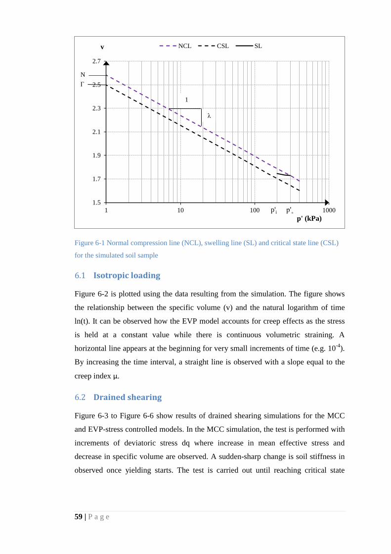
59 | P a g e
Figure 6-1 Normal compression line (NCL), swelling line (SL) and critical state line (CSL)
for the simulated soil sample
Isotropic loading 6.1
Figure 6-2 is plotted using the data resulting from the simulation. The figure shows
the relationship between the specific volume (v) and the natural logarithm of time
ln(t). It can be observed how the EVP model accounts for creep effects as the stress
is held at a constant value while there is continuous volumetric straining. A
horizontal line appears at the beginning for very small increments of time (e.g. 10-4).
By increasing the time interval, a straight line is observed with a slope equal to the
creep index μ.
Drained shearing 6.2
Figure 6-3 to Figure 6-6 show results of drained shearing simulations for the MCC
and EVP-stress controlled models. In the MCC simulation, the test is performed with
increments of deviatoric stress dq where increase in mean effective stress and
decrease in specific volume are observed. A sudden-sharp change is soil stiffness in
observed once yielding starts. The test is carried out until reaching critical state
1.5
1.7
1.9
2.1
2.3
2.5
2.7
1 10 100 1000
v
p' (kPa)
NCL CSL SL
Г N
λ
1
p'i p'˳

60 | P a g e
where continuous shear strains will be developing with no volumetric strains. If the
deviatoric stress is increased beyond this point (crossing the critical state line), shear
strains will reach infinity and then start giving negative values which does not have
any physical meaning. Thus the simulation is stopped at reasonably large value of
shear strain.
Figure 6-2 The relationship between specific volume v and logarithm of time ln(t) after a
sudden increase in mean effective stress p' under isotropic loading
In the EVP stress-controlled simulation, incremental increase in q is applied with
different rates where the higher the rate of shearing, the higher the soil stiffness and
yielding stress will be. At the beginning, only small viscoplastic volumetric strain
increments develop resulting very small dp' (the curve hardly moves). Once the
viscoplastic curve is approached, dramatic increase in dεvvp is observed while the
viscoplastic curve grows with a slower rate. This result in a stress state outside the
viscoplastic curve and very large values of dεvvp developing (the term p′eq/ p′˳ is now
greater than one). However, as the stress point approaches critical state, η keep
increasing and the term (M2−η2
M2 ) approaches zero. As a result, dεvvp/dt slows down
and come to zero at critical state. However, if the simulation continues, stress state
will cross CSL in q:p' plane and result in negative dεvvp/dt.
1.54
1.56
1.58
1.60
1.62
1.64
1.66
1.68
1.70
1.72
1.74
1.E-04 1.E-03 1.E-02 1.E-01 1.E+00 1.E+01 1.E+02 1.E+03 1.E+04 1.E+05 1.E+06
v
ln(t) (d)
μ
1

61 | P a g e
Figure 6-3 q:p’ plane of drained simulation of conventional triaxial test (stress-controlled)
Figure 6-4 v:ln(p’) plane of drained simulation of conventional triaxial test (stress-controlled)
0
50
100
150
200
250
300
0 50 100 150 200 250 300 350
q (kPa)
p' (kPa)
CSL Yeild Curve
EVP-StressC-D-3 kPa/d EVP-StressC-D-30 kPa/d
EVP-StressC-D-300 kPa/d MCC-D
1.62
1.64
1.66
1.68
1.70
1.72
1.74
1.76
1.78
1.80
140 160 180 200 220 240 260 280 300
v
p' (kPa)
CSL NCLEVP-StressC-D-3 kPa/d EVP-StressC-D-30 kPa/dEVP-StressC-D-300 kPa/d MCC-D
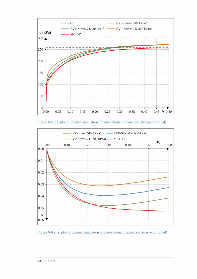
62 | P a g e
Figure 6-5 q:εs plot of drained simulation of conventional triaxial test (stress-controlled)
Figure 6-6 εv:εs plot of drained simulation of conventional triaxial test (stress-controlled)
0
50
100
150
200
250
300
0.00 0.05 0.10 0.15 0.20 0.25 0.30 0.35 0.40 0.45 0.50
q (kPa)
εs
CSL EVP-StressC-D-3 kPa/d
EVP-StressC-D-30 kPa/d EVP-StressC-D-300 kPa/d
MCC-D
0.00
0.01
0.02
0.03
0.04
0.05
0.06
0.00 0.10 0.20 0.30 0.40 0.50 0.60
εv
εs
EVP-StressC-D-3 kPa/d EVP-StressC-D-30 kPa/d
EVP-StressC-D-300 kPa/d MCC-D

63 | P a g e
As a result, volume expansion will be observed in v:ln(p') plane (the compression
plane) as well as dεv:dεs plot. From q:εs plot, it can be seen how the change in
stiffness is smooth and gradual as dεvvp starts developing from the beginning.
Figure 6-7 to Figure 6-10 show results of drained shearing simulations for the EVP-
strain controlled model. For the EVP-strain controlled simulation, shear strain
increments are applied with different rates. As previously said, the higher the strain
rate the higher the soil stiffness and yielding stress will be. Before yielding, peq is
increasing with a rate much faster than rate of increase of dp'. Once yielding is
reached and stress point gets out of the curve, dramatic sharp drop in stiffness is
observed due to the big increase in dεsvp which results in a decrease in dεse (as
constant dεs is applied) and thus a decrease in dq. Once stress state reaches critical
state line, no further decrease in volume is observed and q:εs curve becomes
horizontally asymptotic to CSL.
Figure 6-7 q:p’ plane of drained simulation of conventional triaxial test (strain-controlled)
0
50
100
150
200
250
300
0 50 100 150 200 250 300 350
q (kPa)
p' (kPa)
CSL Yeild Curve
EVP-StrainC-D-0.3 /d EVP-StrainC-D-0.03 /d
EVP-StrainC-D-0.003 /d MCC-D

64 | P a g e
Figure 6-8 v:ln(p’) plane of drained simulation of conventional triaxial test (strain-controlled)
Figure 6-9 q:εs plot of drained simulation of conventional triaxial test (strain-controlled)
1.62
1.64
1.66
1.68
1.70
1.72
1.74
1.76
1.78
1.80
140 160 180 200 220 240 260 280 300
v
p' (kPa)
CSL NCL
EVP-StrainC-D-0.3 /d EVP-StrainC-D-0.03 /d
EVP-StrainC-D-0.003 /d MCC-D
0
50
100
150
200
250
300
0.00 0.05 0.10 0.15 0.20 0.25 0.30 0.35 0.40 0.45 0.50
q (kPa)
εs
CSL EVP-StrainC-D-0.3 /d
EVP-StrainC-D-0.03 /d EVP-StrainC-D-0.003 /d
MCC-D
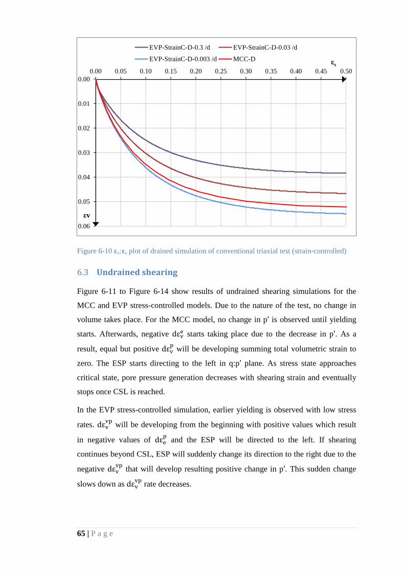
65 | P a g e
Figure 6-10 εv:εs plot of drained simulation of conventional triaxial test (strain-controlled)
Undrained shearing 6.3
Figure 6-11 to Figure 6-14 show results of undrained shearing simulations for the
MCC and EVP stress-controlled models. Due to the nature of the test, no change in
volume takes place. For the MCC model, no change in p’ is observed until yielding
starts. Afterwards, negative dεve starts taking place due to the decrease in p’. As a
result, equal but positive dεvp will be developing summing total volumetric strain to
zero. The ESP starts directing to the left in q:p’ plane. As stress state approaches
critical state, pore pressure generation decreases with shearing strain and eventually
stops once CSL is reached.
In the EVP stress-controlled simulation, earlier yielding is observed with low stress
rates. dεvvp will be developing from the beginning with positive values which result
in negative values of dεep and the ESP will be directed to the left. If shearing
continues beyond CSL, ESP will suddenly change its direction to the right due to the
negative dεvvp that will develop resulting positive change in p’. This sudden change
slows down as dεvvp rate decreases.
0.00
0.01
0.02
0.03
0.04
0.05
0.06
0.00 0.05 0.10 0.15 0.20 0.25 0.30 0.35 0.40 0.45 0.50
εv
εs
EVP-StrainC-D-0.3 /d EVP-StrainC-D-0.03 /d
EVP-StrainC-D-0.003 /d MCC-D
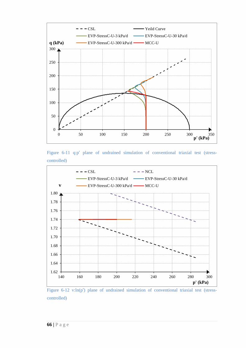
66 | P a g e
Figure 6-11 q:p’ plane of undrained simulation of conventional triaxial test (stress-
controlled)
Figure 6-12 v:ln(p’) plane of undrained simulation of conventional triaxial test (stress-
controlled)
0
50
100
150
200
250
300
0 50 100 150 200 250 300 350
q (kPa)
p' (kPa)
CSL Yeild Curve
EVP-StressC-U-3 kPa/d EVP-StressC-U-30 kPa/d
EVP-StressC-U-300 kPa/d MCC-U
1.62
1.64
1.66
1.68
1.70
1.72
1.74
1.76
1.78
1.80
140 160 180 200 220 240 260 280 300
v
p' (kPa)
CSL NCL
EVP-StressC-U-3 kPa/d EVP-StressC-U-30 kPa/d
EVP-StressC-U-300 kPa/d MCC-U
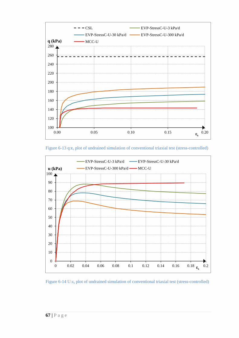
67 | P a g e
Figure 6-13 q:εs plot of undrained simulation of conventional triaxial test (stress-controlled)
Figure 6-14 U:εs plot of undrained simulation of conventional triaxial test (stress-controlled)
100
120
140
160
180
200
220
240
260
280
0.00 0.05 0.10 0.15 0.20
q (kPa)
εs
CSL EVP-StressC-U-3 kPa/d
EVP-StressC-U-30 kPa/d EVP-StressC-U-300 kPa/d
MCC-U
0
10
20
30
40
50
60
70
80
90
100
0 0.02 0.04 0.06 0.08 0.1 0.12 0.14 0.16 0.18 0.2
u (kPa)
εs
EVP-StressC-U-3 kPa/d EVP-StressC-U-30 kPa/d
EVP-StressC-U-300 kPa/d MCC-U
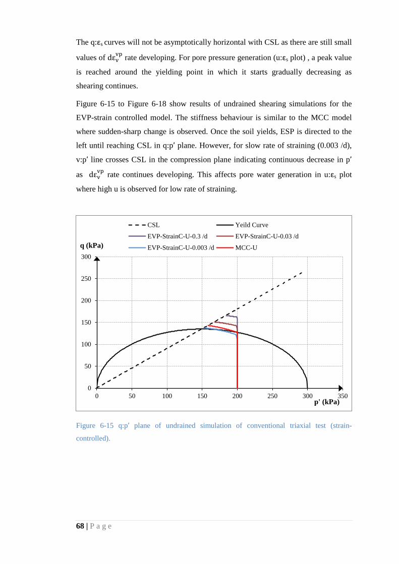
68 | P a g e
The q:εs curves will not be asymptotically horizontal with CSL as there are still small
values of dεvvp rate developing. For pore pressure generation (u:εs plot) , a peak value
is reached around the yielding point in which it starts gradually decreasing as
shearing continues.
Figure 6-15 to Figure 6-18 show results of undrained shearing simulations for the
EVP-strain controlled model. The stiffness behaviour is similar to the MCC model
where sudden-sharp change is observed. Once the soil yields, ESP is directed to the
left until reaching CSL in q:p’ plane. However, for slow rate of straining (0.003 /d),
v:p’ line crosses CSL in the compression plane indicating continuous decrease in p’
as dεvvp rate continues developing. This affects pore water generation in u:εs plot
where high u is observed for low rate of straining.
Figure 6-15 q:p’ plane of undrained simulation of conventional triaxial test (strain-
controlled).
0
50
100
150
200
250
300
0 50 100 150 200 250 300 350
q (kPa)
p' (kPa)
CSL Yeild Curve
EVP-StrainC-U-0.3 /d EVP-StrainC-U-0.03 /d
EVP-StrainC-U-0.003 /d MCC-U
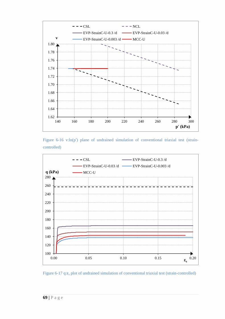
69 | P a g e
Figure 6-16 v:ln(p’) plane of undrained simulation of conventional triaxial test (strain-
controlled)
Figure 6-17 q:εs plot of undrained simulation of conventional triaxial test (strain-controlled)
1.62
1.64
1.66
1.68
1.70
1.72
1.74
1.76
1.78
1.80
140 160 180 200 220 240 260 280 300
v
p' (kPa)
CSL NCL
EVP-StrainC-U-0.3 /d EVP-StrainC-U-0.03 /d
EVP-StrainC-U-0.003 /d MCC-U
100
120
140
160
180
200
220
240
260
280
0.00 0.05 0.10 0.15 0.20
q (kPa)
εs
CSL EVP-StrainC-U-0.3 /d
EVP-StrainC-U-0.03 /d EVP-StrainC-U-0.003 /d
MCC-U
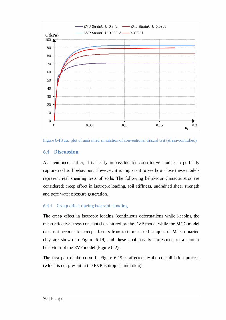
70 | P a g e
Figure 6-18 u:εs plot of undrained simulation of conventional triaxial test (strain-controlled)
Discussion 6.4
As mentioned earlier, it is nearly impossible for constitutive models to perfectly
capture real soil behaviour. However, it is important to see how close these models
represent real shearing tests of soils. The following behaviour characteristics are
considered: creep effect in isotropic loading, soil stiffness, undrained shear strength
and pore water pressure generation.
6.4.1 Creep effect during isotropic loading
The creep effect in isotropic loading (continuous deformations while keeping the
mean effective stress constant) is captured by the EVP model while the MCC model
does not account for creep. Results from tests on tested samples of Macau marine
clay are shown in Figure 6-19, and these qualitatively correspond to a similar
behaviour of the EVP model (Figure 6-2).
The first part of the curve in Figure 6-19 is affected by the consolidation process
(which is not present in the EVP isotropic simulation).
0
10
20
30
40
50
60
70
80
90
100
0 0.05 0.1 0.15 0.2
u (kPa)
εs
EVP-StrainC-U-0.3 /d EVP-StrainC-U-0.03 /d
EVP-StrainC-U-0.003 /d MCC-U

71 | P a g e
Figure 6-19 Vertical displacement vs. logarithm of time of Macau marine clay (Lok and Shi,
2008)
However, as consolidation continues and excess pore water dissipates, the curve
becomes close to a straight line in a similar fashion to Figure 6-2.
6.4.2 Soil stiffness
The MCC model predicts a sudden-sharp change in stiffness once yielding is reached
(Figure 6-15 & Figure 6-17). This is because the model assumes that plastic strains
start developing only when yielding is reached. EVP model assumes continuous
viscoplastic strains taking place even inside the viscoplastic curve. Thus, the model
predicts gradual change in stiffness in the stress-controlled simulation (Figure 6-3,
Figure 6-5, Figure 6-11 & Figure 6-13) which rounds the sharp change of the MCC
model. This prediction is much closer to real soil behaviour where gradual-smooth
change in stiffness is observed (Figure 6-20). However, strain-controlled simulation
of the EVP model predicts a sudden-sharp change in stiffness in a similar manner to
the MCC model.
6.4.3 Undrained shear strength
In Section 2.2, data from Drammen clay were presented in which different samples
were sheared at different strain rates in undrained triaxial test (Figure 2-10). It was

72 | P a g e
shown how the undrained shear strength of the soil differs with shearing rate where
the higher the shearing rate the higher the value of cu will be. Furthermore, Rowe &
Hinchberger (1998) performed undrained triaxial tests with different strain rates on
overconsolidated samples of Sackville soil taken from a depth of 3.65-3.85 m
(Figure 6-20). The same relationship between shearing rate and cu is observed. This
important effect of rate of shearing was perfectly matched by the EVP model (stress
controlled and strain controlled) as shown in Figure 6-13 & Figure 6-17 respectively.
On the other hand, the MCC model does not account for shearing rate effects.
Figure 6-20 Measured deviatoric stress versus axial strain response during undrained triaxial
test (Rowe and Hinchberger, 1998)
6.4.4 Pore water pressure generation
The pore pressure generated during an undrained compression triaxial test is directly
related to the rate of shearing. For a normally consolidated or lightly
overconsolidated sample, the higher the shearing rate the lower the pore pressure will
be. This effect is well captured by the EVP model in the undrained test (Figure 6-14

73 | P a g e
& Figure 6-18). The EVP model simulated the relationship between u and εs in close
way to the observed real soil behaviour under undrained shearing (Figure 6-21). It
can be seen from the figure how pore water pressure reaches a peak value and then
starts decreasing with shear strains which corresponds to similar behaviour in stress-
controlled simulation of the EVP model.
Figure 6-21 Pore water pressure vs. axial strain in a triaxial compression undrained test of
Dog’s Bay sand with different straining rates (García, 2011)
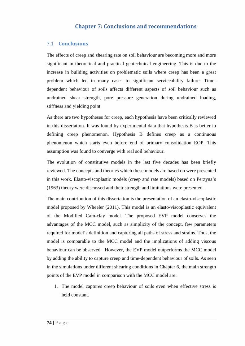
74 | P a g e
Chapter 7: Conclusions and recommendations 7
Conclusions 7.1
The effects of creep and shearing rate on soil behaviour are becoming more and more
significant in theoretical and practical geotechnical engineering. This is due to the
increase in building activities on problematic soils where creep has been a great
problem which led in many cases to significant serviceability failure. Time-
dependent behaviour of soils affects different aspects of soil behaviour such as
undrained shear strength, pore pressure generation during undrained loading,
stiffness and yielding point.
As there are two hypotheses for creep, each hypothesis have been critically reviewed
in this dissertation. It was found by experimental data that hypothesis B is better in
defining creep phenomenon. Hypothesis B defines creep as a continuous
phenomenon which starts even before end of primary consolidation EOP. This
assumption was found to converge with real soil behaviour.
The evolution of constitutive models in the last five decades has been briefly
reviewed. The concepts and theories which these models are based on were presented
in this work. Elasto-viscoplastic models (creep and rate models) based on Perzyna’s
(1963) theory were discussed and their strength and limitations were presented.
The main contribution of this dissertation is the presentation of an elasto-viscoplastic
model proposed by Wheeler (2011). This model is an elasto-viscoplastic equivalent
of the Modified Cam-clay model. The proposed EVP model conserves the
advantages of the MCC model, such as simplicity of the concept, few parameters
required for model’s definition and capturing all paths of stress and strains. Thus, the
model is comparable to the MCC model and the implications of adding viscous
behaviour can be observed. However, the EVP model outperforms the MCC model
by adding the ability to capture creep and time-dependent behaviour of soils. As seen
in the simulations under different shearing conditions in Chapter 6, the main strength
points of the EVP model in comparison with the MCC model are:
1. The model captures creep behaviour of soils even when effective stress is
held constant.
75 | P a g e
2. The model presents the effect of shearing rate on the following properties:
a. undrained shear strength which increases with rate of shearing;
b. pore water pressure generation during undrained shearing, which
decreases with shearing rate;
c. volumetric strain during drained shearing, which decreases with
shearing rate;
d. the yielding stress which increases with the shearing rate.
3. When considering real soil behaviour (Section 6.4), the EVP model provides
very good qualitative representation of this behaviour.
Recommendations for further work 7.2
The effect of anisotropy was kept out of the scope of this work in order to keep the
proposed EVP model comparable to the MCC model under consideration. However,
the effect of anisotropy can be included in the future to the EVP model and then
compare it with other elastoplastic models that account for anisotropy (e.g. Dafalias
1986 model). (Dafalias, 1986)
For the strain-controlled EVP simulations, a sharp change in stiffness was observed
which deviates from real soil behaviour. If this change is to be smoother, the value of
the creep index μ needs to increase in order to get slower build-up of the creep
volumetric strains as shown in Equation 4.12.
The proposed EVP model is relatively simple compared with other elasto-
viscoplastic models. This makes the EVP model easier to understand especially for
those used to the MCC model. The model is worth being explored further with
quantitative numerical predictions and comparisons against experimental results in
which afterwards full framework of the model will be set up along with a name for it
(e.g. Wheeler 2011 model).

76 | P a g e
References
Aboshi, H. (1973) 'An experimental investigation on the similitude in the
consolidation of a soft clay, including the secondary creep settlement', Proceeding of
8th International Conference on Soil Mechanics and Geotechnical Engineering,
Moscow, 88.
Adachi, T. and Oka, F. (1982) 'Constitutive equations for normally consolidated clay
based on elasto-viscoplasticity', Soils and Foundations, vol. 22, no. 4, pp. 57-70.
Atkinson, (1993) Introduction to the Mechanics of Soils and Foundations: Through
Critical State Soil Mechanics, London: McGraw-Hill Book Company.
Bažant, P. (1985) Mechanics of Geomaterials: Rocks, Concretes and Soils, Chester,
New York: Wiley & Sons.
Berre, T. and Bjerrum, L. (1973) 'Shear strength of normally consolidated clays',
International conference on Soil Mechanics and Foundation Engineering, Moskow,
39-49.
Bjerrum, L. (1967) 'Engineering geology of Norwegian normally-consolidated
marine clays as related to settlements of buildings', Géotechnique, vol. 17, no. 2, pp.
83-118.
Borja, R.I. and Kavazanjian, E. (1985) 'A constitutive model for the stress-strain-
time behaviour of 'wet' clays', Geotechnique, vol. 35, no. 3, pp. 283-298.
Dafalias, Y.F. (1986) 'An anisotropic critical state soil plasticity model', Mechanics
Research Communications, vol. 13, p. 341–347.
Das, B.M. (2010) Principles of Foundation Engineering, 7th edition, Cengage
Learning.
Degago, S.A., Grimstad, G., Jostad, H.P., Nordal, S. and Olsson, M. (2010) 'Use and
misuse of the isotache concept with respect to creep hypotheses A and B',
Géotechnique, vol. 61, no. 10, p. 897 –908.
77 | P a g e
Dolezalova, M., Zemanova, V. and Danko, J. (1998) 'An approach for selecting rock
mass constitutive model for surface settlement predictions', Proceedings of 1st
International Conference on Soil–Structure Interaction in Urban Civil Engineering,
Darmstadt, 44-66.
Drucker, D.C., Gibson, R.E. and Henkel, D.J. (1957) 'Soil mechanics and work
hardening theories of plasticity', Transactions of the American Society of Civil
Engineers, vol. 122, p. 338–349.
Drucker, D.C. and Prager, W. (1952) 'Soil mechanics and plasticity analysis or limit
design', Quarterly of Applied Mathematics, vol. 10, no. 2, p. 157–165.
Duncan, J.M. and Chang, C.Y. (1970) 'Nonlinear analysis of stress and strain in
soils', Soil Mechanics and Foundation Division, Proceedings of ASCE, vol. 96, pp.
1629-1653.
García, A., (2011) 'Loading Rate Effects on Dog's Bay Sand', Civil Engineering
Gradaution Research Work, Technical University of Catalonia, Spain.
Graham, J., Crooks, J.H.A. and Bell, A.L. (1983) 'Time effects on the stress-strain
behaviour of natural soft clays', Géotechnique, vol. 33, no. 3, pp. 327-340.
Graham, J., Noonan, M.L. and Lew, K.V. (1983) 'Yield states and stress-strain
relationships in a natural plastic clay', Canadian Geotechnial Journal, vol. 20, no. 3,
pp. 502-516.
Havel, F. (2004) Creep in soft soils, Ph.D. Thesis. Norwegian University of Science
and Technology NTNU: Trondheim.
Janbu, N. (1696) 'The resistance concept applied to deformations of soils',
Proceeding on the 7th International Conference on Soil Mechanics and Foundation
Engineering, Mexico City, 191-196.
Jardine, R.J., Potts, D.M., Fourie, A.B. and Burland, J.B. (1986) 'Studies of the
influence of non-linear stress–strain characteristics in soil–structure interaction',
Géotechnique, vol. 36, no. 3, p. 377–396.
Karim, R. and Gnanendran, C.T. (2008) 'Review of Visco-plastic soil models for
predicting the performance of embankments on soft soils', The 12th International
78 | P a g e
Conference of International Association for Computer Methods and Advances in
Geomechanics (IACMAG), Goa, 945-956.
Karim, M.R., Gnanendran, C.T., Lo, S.-C.R. and Mak, J. (2010) 'Predicting the long
term performance of a wide embankment on soft soil using an elasto-viscoplastic
model', Canadian Geotechnical Journal, vol. 47, no. 2, pp. 244-257.
Kondne, R. (1963) 'Hyperbolic stress–strain response: cohesive soils', ASCE Soil
Mechanics and Foundation Division, vol. 89, p. 115–143.
Konovalov, P.A. and Bezvolev, S.G. (2005) 'Analysis of results of consolidation
tests of saturated clayey soils', Soil Mechanics and Foundation Engineering, vol. 42,
no. 3, pp. 81-85.
Ladd, C.C. and DeGroot, D.J. (2003) 'Recommended Practice for Soft Ground Site
Characterization: Arthur Casagrande Lecture', 12th Panamerican Conference on Soil
Mechanics and Geotechnical Engineering, Cambridge MA.
Ladd, C.C., Foott, R., Ishihara, K., Schlosser, F. and Poulos, H.G. (1977) 'Stress-
deformation and strength characteristics. State-of-the-art report', Proceeding of the
9th International Conference on Soil Mechancis and Foundation Engineering, Tokyo,
421–494.
Leroueil, S. (1994) 'Compressibility of Clays: fundamental and practical aspects',
ASCE Geotechnical Special Publication, vol. 40, no. 1, pp. 57-76.
Leroueil, S. (2006) 'The isotache approach. Where are we 50 years after its
development by Professor Šuklje? (2006 Prof. Šuklje's Memorial Lecture)',
Proceeding on the 13th Danube European Conference on Geotechnical Engineering,
Ljubljana, 55-88.
Lok, T.M. and Shi, X. (2008) 'Report: Consolidation and Strength Properties of
Macau Marine Clay', Faculty of Science and Technology, University of Macau.
Malvern, L.E. (1951) 'The propagation of longitudinal waves of plastic deformation
in a bar of metal exhibiting a strain rate effect', Journal of Applied Mechanics, vol.
18, pp. 203-208.

79 | P a g e
Marchi, M., Butterfield, R., Gottardi, G. and Lancellotta, R. (2011) 'Stability and
strength analysis of leaning towers', Géotechnique, vol. 61, no. 12, p. 1069 –1079.
Mesri, G. (2003) 'Primary and secondary compression', ASCE Geotechnical special
publication 119, p. 122–166.
Mesri, G. and Godlewski, P.M. (1977) 'Time and stress-compressibility
interrelationship', ASCE Journal Geotechnical Engineering, vol. 103, pp. 417-430.
Nash, D.F.T. (2010) 'Influence of destruction of soft clay on time-dependant
settlements', Proceeding on the 7th European Conference Numerical methods in
Geotechnical Engineering, Trondheim, 75-80.
Perzyna, P. (1963) 'The constitutive equations for rate sensitivity plastic materials',
Quarterly of Applied Mathematics, vol. 20, no. 4, pp. 321-332.
Perzyna, P. (1966) 'Fundamental problems in viscoplasticity', Advances in Applied
Mechanics, vol. 9, pp. 244-368.
Potts, , Axelsson, K., Grande, L., Schweiger , H.F. and Long, (ed.) (2002) Guidelines
for the Use of Advanced Numerical Analysis, London: Thomas Telford Ltd.
Potts, D.M. and Zdravkovic, L. (1999) Finite Element Analysis in Geotechnical
Engineering Volume One - Theory, ICE Publishing.
Prevost, J.H. and Popsecu, R. (1996) 'Constitutive relations for soil materials',
Electronic Journal of Geotechnical Engineering, vol. 1, November.
Puzrin, M. (2012) Constitutive Modelling in Geomechanics: Introduction, Springer.
Richardson, A.M. and Whitman, R.V. (1963) 'Effect of strain-rate upon drained
shear resistance of a saturated remoulded fat clay', Géotechnique, vol. 13, no. 4, pp.
310-324.
Roscoe , K.H. and Burland, J.B. (1968) 'On the Generalized Stress-Strain Behavior
of Wet Clay', Engineering Plasticity, Cambridge University Press, pp. 535-609.
Roscoe, K.H. and Schofield, A.N. (1963) 'Mechanical behaviour of an idealised
‘wet’ clay', European Conference for Soil Mechanics and Foundation Engineering,
Wiesbaden, 47–54.
80 | P a g e
Rowe, R.K. and Hinchberger, S.D. (1998) 'The significance of rate effects in the
modeling the Sackville test embankment', Canadian Geotechnical Journal, vol. 35,
pp. 500-516.
Schofield, A.N. and Wroth, C.P. (1968) Critical State Soil Mechanics, London:
McGraw-Hill.
Sekiguchi, H. (1977) 'Rheological Characteristics of Clays', Proceedings of the 9th
International Conference on Soil Mechanics and Foundation Engineering, Tokyo,
289-292.
Smoltczyk, U. (2002) Handbook of Geotechnical Engineering Practice, Berlin:
Wiley-VCH.
Šuklje, L. (1957) 'The analysis of the consolidation process by the isotaches method',
Proceeding on the 4th International Conference on Soil Mechanics and Foundation
Engineering, London, 202-206.
Tavenas, F., Leroueil, S., LaRochelle, P. and Roy, M. (1978) 'Creep behaviour of an
undisturbed lightly overconsolidated clay', Canadian Geotechnical Journal, vol. 15,
no. 3, pp. 402-423.
Vermeer, P.A. and Neher, H.P. (1999) 'A soft soil model that account for creep',
Beyond 2000 in computational geotechnics: 10 Years of Plaxis International,
Rotterdam, 249-261.
Wheeler, S.J. (2011) Personal communication. University of Glasgow.
Wood, , (1990) Soil Behaviour and Critical State Soil Mechanics, Cambridge
University Press.
Yu, H.S. (1998) 'CASM: A unified state parameter model for clay and sand',
International Journal of Numerical and Analytical Methods in Geomechanics, vol.
22, no. 8, pp. 621-653.
Zienkiewicz, O.C. and Naylor, D.J. (1973) 'Finite element studies of soils and porous
media', Lecture: Finite elements in continuum mechanics, p. 459–493.
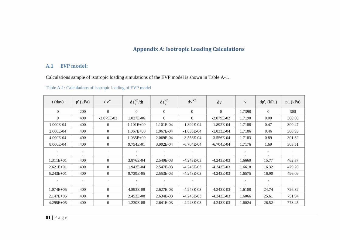
81 | P a g e
A. Appendix A: Isotropic Loading Calculations
A.1 EVP model:
Calculations sample of isotropic loading simulations of the EVP model is shown in Table A-1.
Table A-1: Calculations of isotropic loading of EVP model
t (day) p' (kPa) dve dεvvp/dt dεv
vp dvvp dv v dp'˳ (kPa) p'˳ (kPa)
0 200 0 0 0 0 0 1.7398 0 300 0 400 -2.079E-02 1.037E-06 0 0 -2.079E-02 1.7190 0.00 300.00
1.000E-04 400 0 1.101E+00 1.101E-04 -1.892E-04 -1.892E-04 1.7188 0.47 300.47 2.000E-04 400 0 1.067E+00 1.067E-04 -1.833E-04 -1.833E-04 1.7186 0.46 300.93 4.000E-04 400 0 1.035E+00 2.069E-04 -3.556E-04 -3.556E-04 1.7183 0.89 301.82 8.000E-04 400 0 9.754E-01 3.902E-04 -6.704E-04 -6.704E-04 1.7176 1.69 303.51
.
. . .
.
. . .
.
. . .
.
. . .
.
. . .
1.311E+01 400 0 3.876E-04 2.540E-03 -4.243E-03 -4.243E-03 1.6660 15.77 462.87 2.621E+01 400 0 1.943E-04 2.547E-03 -4.243E-03 -4.243E-03 1.6618 16.32 479.20 5.243E+01 400 0 9.739E-05 2.553E-03 -4.243E-03 -4.243E-03 1.6575 16.90 496.09
.
. . .
.
. . .
.
. . .
.
. . .
.
. . .
1.074E+05 400 0 4.893E-08 2.627E-03 -4.243E-03 -4.243E-03 1.6108 24.74 726.32 2.147E+05 400 0 2.453E-08 2.634E-03 -4.243E-03 -4.243E-03 1.6066 25.61 751.94 4.295E+05 400 0 1.230E-08 2.641E-03 -4.243E-03 -4.243E-03 1.6024 26.52 778.45

82 | P a g e
t (day) p' (kPa) dve dεvvp/dt dεv
vp dvvp dv v dp'˳ (kPa) p'˳ (kPa)
8.590E+05 400 0 6.165E-09 2.648E-03 -4.243E-03 -4.243E-03 1.5981 27.45 805.90 . .
.
. . .
.
. . .
.
. . .
.
. . .
.
. 1.100E+08 400 0 4.908E-11 2.698E-03 -4.243E-03 -4.243E-03 1.5684 34.99 1027.17
2.199E+08 400 0 2.461E-11 2.705E-03 -4.243E-03 -4.243E-03 1.5642 36.22 1063.39
4.398E+08 400 0 1.234E-11 2.713E-03 -4.243E-03 -4.243E-03 1.5599 37.50 1100.89
8.796E+08 400 0 6.185E-12 2.720E-03 -4.243E-03 -4.243E-03 1.5557 38.82 1139.72

83 | P a g e
B. Appendix B: Drained Shearing Calculations
B.1 MCC model – stress controlled:
Calculations sample of drained shearing simulations of the MCC model is shown in Table B-1.
Table B-1 Calculations of stress-controlled drained shearing of the MCC model
p' (kPa)
q (kPa)
p'eq (kPa)
p'˳ (kPa) dεve dεse dεv
p dεsp dεv dεs εv εs dv v
200 0 200 300 0 0 0 0 0 0 0 0 0 1.7398
201 3 201.1 300.0 8.622E-05
1.000E-04 0.000E+00 0.000E+00 8.622E-
05 1.000E-04 8.622E-05 1.000E-04 -1.500E-
04 1.7396
202 6 202.2 300.0 8.580E-05
1.000E-04 0.000E+00 0.000E+00 8.580E-
05 1.000E-04 1.720E-04 2.000E-04 -1.493E-
04 1.7395
203 9 203.5 300.0 8.538E-05
1.000E-04 0.000E+00 0.000E+00 8.538E-
05 1.000E-04 2.574E-04 3.000E-04 -1.485E-
04 1.7393
204 12 204.9 300.0 8.497E-05
1.000E-04 0.000E+00 0.000E+00 8.497E-
05 1.000E-04 3.424E-04 4.000E-04 -1.478E-
04 1.7392
205 15 206.4 300.0 8.456E-05
1.000E-04 0.000E+00 0.000E+00 8.456E-
05 1.000E-04 4.269E-04 5.000E-04 -1.471E-
04 1.7390
206 18 207.9 300.0 8.415E-05
1.000E-04 0.000E+00 0.000E+00 8.415E-
05 1.000E-04 5.111E-04 6.000E-04 -1.463E-
04 1.7389
207 21 209.6 300.0 8.375E-05
1.000E-04 0.000E+00 0.000E+00 8.375E-
05 1.000E-04 5.948E-04 7.000E-04 -1.456E-
04 1.7387
208 24 211.4 300.0 8.335E-05
1.000E-04 0.000E+00 0.000E+00 8.335E-
05 1.000E-04 6.782E-04 8.000E-04 -1.449E-
04 1.7386
.
. . .
.
. . .
.
. . .
.
. . .
.
. . .
.
. . .
.
. . .
251 153 366.1 366.1 7.015E-05
1.000E-04 9.768E-04 2.605E-03 1.047E-
03 2.705E-03 1.791E-02 3.401E-02 -1.791E-
03 1.7089
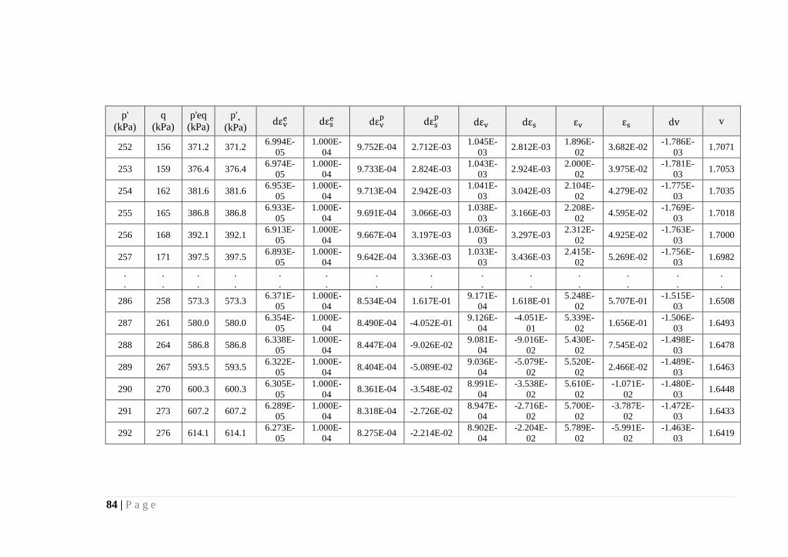
84 | P a g e
p' (kPa)
q (kPa)
p'eq (kPa)
p'˳ (kPa) dεve dεse dεv
p dεsp dεv dεs εv εs dv v
252 156 371.2 371.2 6.994E-05
1.000E-04 9.752E-04 2.712E-03 1.045E-
03 2.812E-03 1.896E-02 3.682E-02 -1.786E-
03 1.7071
253 159 376.4 376.4 6.974E-05
1.000E-04 9.733E-04 2.824E-03 1.043E-
03 2.924E-03 2.000E-02 3.975E-02 -1.781E-
03 1.7053
254 162 381.6 381.6 6.953E-05
1.000E-04 9.713E-04 2.942E-03 1.041E-
03 3.042E-03 2.104E-02 4.279E-02 -1.775E-
03 1.7035
255 165 386.8 386.8 6.933E-05
1.000E-04 9.691E-04 3.066E-03 1.038E-
03 3.166E-03 2.208E-02 4.595E-02 -1.769E-
03 1.7018
256 168 392.1 392.1 6.913E-05
1.000E-04 9.667E-04 3.197E-03 1.036E-
03 3.297E-03 2.312E-02 4.925E-02 -1.763E-
03 1.7000
257 171 397.5 397.5 6.893E-05
1.000E-04 9.642E-04 3.336E-03 1.033E-
03 3.436E-03 2.415E-02 5.269E-02 -1.756E-
03 1.6982
.
. . .
.
. . .
.
. . .
.
. . .
.
. . .
.
. . .
.
. . .
286 258 573.3 573.3 6.371E-05
1.000E-04 8.534E-04 1.617E-01 9.171E-
04 1.618E-01 5.248E-02 5.707E-01 -1.515E-
03 1.6508
287 261 580.0 580.0 6.354E-05
1.000E-04 8.490E-04 -4.052E-01 9.126E-
04 -4.051E-
01 5.339E-
02 1.656E-01 -1.506E-03 1.6493
288 264 586.8 586.8 6.338E-05
1.000E-04 8.447E-04 -9.026E-02 9.081E-
04 -9.016E-
02 5.430E-
02 7.545E-02 -1.498E-03 1.6478
289 267 593.5 593.5 6.322E-05
1.000E-04 8.404E-04 -5.089E-02 9.036E-
04 -5.079E-
02 5.520E-
02 2.466E-02 -1.489E-03 1.6463
290 270 600.3 600.3 6.305E-05
1.000E-04 8.361E-04 -3.548E-02 8.991E-
04 -3.538E-
02 5.610E-
02 -1.071E-
02 -1.480E-
03 1.6448
291 273 607.2 607.2 6.289E-05
1.000E-04 8.318E-04 -2.726E-02 8.947E-
04 -2.716E-
02 5.700E-
02 -3.787E-
02 -1.472E-
03 1.6433
292 276 614.1 614.1 6.273E-05
1.000E-04 8.275E-04 -2.214E-02 8.902E-
04 -2.204E-
02 5.789E-
02 -5.991E-
02 -1.463E-
03 1.6419

85 | P a g e
B.2 EVP model – stress controlled:
Calculations sample of drained shearing simulations of the stress-controlled EVP model with dq/dt = 3 kPa/d is shown in Table B-1.
Table B-2: Calculations of stress-controlled (3 kPa/d) drained shearing of EVP model
t (day
)
p' (kPa
)
q (kPa
)
p'eq (kPa) dεve dεse dεv
vp
/dt dεvvp dεs
vp/dt dεsvp dεv dεs εv εs dv v
dp'˳ (kPa
)
p'˳ (kPa)
0 200 0 200 0 0 0 0 0 0 0 0 0 0 0 1.73977 0 300
1 201 3 201.06
8.622E-05
1.000E-04
1.037E-06
1.037E-06
0.000E+00
0.000E+00
8.726E-05
1.000E-04
8.726E-05
1.000E-04
-1.518E-04
1.73962 0.00 300.0
0
2 202 6 202.22
8.580E-05
1.000E-04
1.152E-06
1.152E-06
4.245E-08
4.245E-08
8.695E-05
1.000E-04
1.742E-04
2.000E-04
-1.513E-04
1.73947 0.01 300.0
1
3 203 9 203.49
8.538E-05
1.000E-04
1.291E-06
1.291E-06
9.481E-08
9.481E-08
8.667E-05
1.001E-04
2.609E-04
3.001E-04
-1.508E-04
1.73932 0.01 300.0
2
.
. . .
.
. . .
.
. . .
.
. . .
.
. . .
.
. . .
.
. . .
.
. . .
.
. . .
31 231 93 277.22
7.525E-05
1.000E-04
3.020E-04
3.020E-04
3.598E-04
3.598E-04
3.773E-04
4.598E-04
4.106E-03
4.712E-03
-6.539E-04
1.73264 1.33 307.0
6
32 232 96 281.04
7.495E-05
1.000E-04
3.586E-04
3.586E-04
4.456E-04
4.456E-04
4.335E-04
5.456E-04
4.539E-03
5.258E-03
-7.511E-04
1.73189 1.59 308.6
5
33 233 99 284.93
7.466E-05
1.000E-04
4.193E-04
4.193E-04
5.433E-04
5.433E-04
4.940E-04
6.433E-04
5.033E-03
5.901E-03
-8.556E-04
1.73104 1.87 310.5
2
34 234 102 288.89
7.438E-05
1.000E-04
4.824E-04
4.824E-04
6.512E-04
6.512E-04
5.568E-04
7.512E-04
5.590E-03
6.652E-03
-9.638E-04
1.73007 2.16 312.6
8
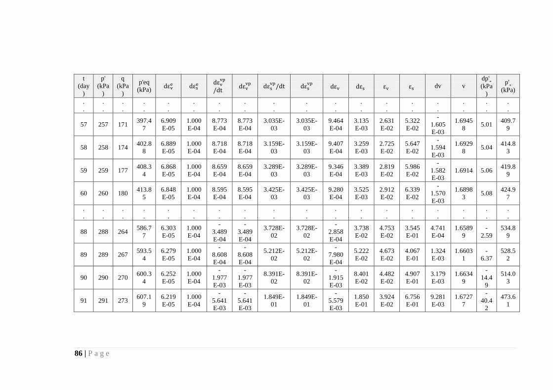
86 | P a g e
t (day
)
p' (kPa
)
q (kPa
)
p'eq (kPa) dεve dεse dεv
vp
/dt dεvvp dεs
vp/dt dεsvp dεv dεs εv εs dv v
dp'˳ (kPa
)
p'˳ (kPa)
.
. . .
.
. . .
.
. . .
.
. . .
.
. . .
.
. . .
.
. . .
.
. . .
.
. . .
57 257 171 397.47
6.909E-05
1.000E-04
8.773E-04
8.773E-04
3.035E-03
3.035E-03
9.464E-04
3.135E-03
2.631E-02
5.322E-02
-1.605E-03
1.69458 5.01 409.7
9
58 258 174 402.88
6.889E-05
1.000E-04
8.718E-04
8.718E-04
3.159E-03
3.159E-03
9.407E-04
3.259E-03
2.725E-02
5.647E-02
-1.594E-03
1.69298 5.04 414.8
3
59 259 177 408.34
6.868E-05
1.000E-04
8.659E-04
8.659E-04
3.289E-03
3.289E-03
9.346E-04
3.389E-03
2.819E-02
5.986E-02
-1.582E-03
1.6914 5.06 419.89
60 260 180 413.85
6.848E-05
1.000E-04
8.595E-04
8.595E-04
3.425E-03
3.425E-03
9.280E-04
3.525E-03
2.912E-02
6.339E-02
-1.570E-03
1.68983 5.08 424.9
7
.
. . .
.
. . .
.
. . .
.
. . .
.
. . .
.
. . .
.
. . .
.
. . .
.
. . .
88 288 264 586.77
6.303E-05
1.000E-04
-3.489E-04
-3.489E-04
3.728E-02
3.728E-02
-2.858E-04
3.738E-02
4.753E-02
3.545E-01
4.741E-04
1.65899
-2.59
534.89
89 289 267 593.54
6.279E-05
1.000E-04
-8.608E-04
-8.608E-04
5.212E-02
5.212E-02
-7.980E-04
5.222E-02
4.673E-02
4.067E-01
1.324E-03
1.66031
-6.37
528.52
90 290 270 600.34
6.252E-05
1.000E-04
-1.977E-03
-1.977E-03
8.391E-02
8.391E-02
-1.915E-03
8.401E-02
4.482E-02
4.907E-01
3.179E-03
1.66349
-14.4
9
514.03
91 291 273 607.19
6.219E-05
1.000E-04
-5.641E-03
-5.641E-03
1.849E-01
1.849E-01
-5.579E-03
1.850E-01
3.924E-02
6.756E-01
9.281E-03
1.67277
-40.4
2
473.61

87 | P a g e
B.3 EVP model – strain controlled:
Calculations sample of drained shearing simulations of the strain-controlled EVP model with dεs/dt = 0.3 /d is shown in Table B-3.
Table B-3: Calculations of strain-controlled (0.3 /d) drained shearing of EVP model
t (day
) εs dεs dεs
vp/dt dεsvp dεse
dq (kPa
)
q (kPa
)
p' (kPa
) dεve dεv
vp
/dt dεvvp
p'eq (kPa
) dεv εv dv v
dp'˳ (kPa
) p'˳ (kPa)
0 0 0 0 0 0 0 0 200 0 0 0 200.0
0 0 0
0.000E+
00
1.739
8 0 300
0.00
1
3.000
E-04
3.000
E-04
0.000E+
00
0.000E+
00
3.000
E-04 9.00 9.00
203.0
0
2.587
E-04
1.037
E-06
1.037
E-09
203.4
9
2.587
E-04
2.587
E-04
-4.500E-
04
1.739
3
4.51
E-06
300.0000
05
0.00
2
6.000
E-04
3.000
E-04
1.605E-
07
1.605E-
10
3.000
E-04 9.00 18.00
206.0
0
2.549
E-04
1.463
E-06
1.463
E-09
207.9
4
2.549
E-04
5.136
E-04
-4.434E-
04
1.738
9
6.36
E-06
300.0000
11
.
. . .
.
. . .
.
. . .
.
. . .
.
. . .
.
. . .
.
. . .
.
. . .
.
. . .
.
.
0.64 1.920
E-01
3.000
E-04
2.983E-
01
2.983E-
04
1.685
E-06 0.05
237.5
6
279.1
9
1.075
E-06
1.511
E-02
1.511
E-05
528.7
5
1.618
E-05
3.270
E-02
-2.725E-
05
1.683
8 0.093 439.77
0.64
1
1.923
E-01
3.000
E-04
2.983E-
01
2.983E-
04
1.681
E-06 0.05
237.6
1
279.2
0
1.073
E-06
1.507
E-02
1.507
E-05
528.8
6
1.614
E-05
3.271
E-02
-2.718E-
05
1.683
8 0.093 439.87
0.64
2
1.926
E-01
3.000
E-04
2.983E-
01
2.983E-
04
1.676
E-06 0.05
237.6
6
279.2
2
1.070
E-06
1.503
E-02
1.503
E-05
528.9
6
1.610
E-05
3.273
E-02
-2.710E-
05
1.683
7 0.093 439.96
.
. . .
.
. . .
.
. . .
.
. . .
.
. . .
.
. . .
.
. . .
.
. . .
.
. . .
.
. 1.28 3.840 3.000 2.997E- 2.997E- 3.238 0.01 253.3 284.4 2.038 2.823 2.823 563.0 3.027 3.768 -5.072E- 1.675 0.019 469.36
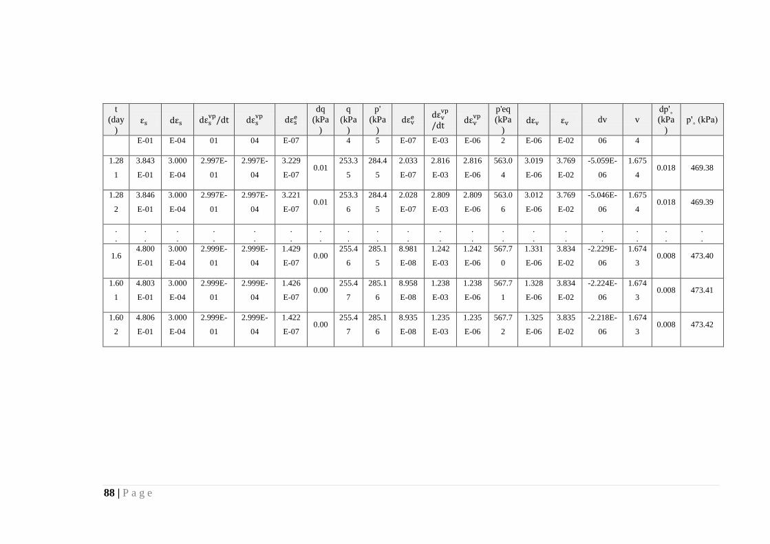
88 | P a g e
t (day
) εs dεs dεs
vp/dt dεsvp dεse
dq (kPa
)
q (kPa
)
p' (kPa
) dεve dεv
vp
/dt dεvvp
p'eq (kPa
) dεv εv dv v
dp'˳ (kPa
) p'˳ (kPa)
E-01 E-04 01 04 E-07 4 5 E-07 E-03 E-06 2 E-06 E-02 06 4
1.28
1
3.843
E-01
3.000
E-04
2.997E-
01
2.997E-
04
3.229
E-07 0.01
253.3
5
284.4
5
2.033
E-07
2.816
E-03
2.816
E-06
563.0
4
3.019
E-06
3.769
E-02
-5.059E-
06
1.675
4 0.018 469.38
1.28
2
3.846
E-01
3.000
E-04
2.997E-
01
2.997E-
04
3.221
E-07 0.01
253.3
6
284.4
5
2.028
E-07
2.809
E-03
2.809
E-06
563.0
6
3.012
E-06
3.769
E-02
-5.046E-
06
1.675
4 0.018 469.39
.
. . .
.
. . .
.
. . .
.
. . .
.
. . .
.
. . .
.
. . .
.
. . .
.
. . .
.
.
1.6 4.800
E-01
3.000
E-04
2.999E-
01
2.999E-
04
1.429
E-07 0.00
255.4
6
285.1
5
8.981
E-08
1.242
E-03
1.242
E-06
567.7
0
1.331
E-06
3.834
E-02
-2.229E-
06
1.674
3 0.008 473.40
1.60
1
4.803
E-01
3.000
E-04
2.999E-
01
2.999E-
04
1.426
E-07 0.00
255.4
7
285.1
6
8.958
E-08
1.238
E-03
1.238
E-06
567.7
1
1.328
E-06
3.834
E-02
-2.224E-
06
1.674
3 0.008 473.41
1.60
2
4.806
E-01
3.000
E-04
2.999E-
01
2.999E-
04
1.422
E-07 0.00
255.4
7
285.1
6
8.935
E-08
1.235
E-03
1.235
E-06
567.7
2
1.325
E-06
3.835
E-02
-2.218E-
06
1.674
3 0.008 473.42

89 | P a g e
C. Appendix C: Undrained Shearing Calculations
C.1 MCC model:
Calculations sample of undrained shearing simulations of the MCC model is shown in Table C-1.
Table C-1: Calculations of undrained shearing of the MCC model
p' (kPa) dεve dεvp dp'˳ (kPa) p'˳ (kPa) q (kPa) dεse dεs
p dεs εs p (kPa) u (kPa) v
200 0 0 0 300 0 0 0 0 0 200 0 1.7398 200 0.000E+00 0.000E+00 0 300.00 127.28 4.243E-03 0.000E+00 4.243E-03 4.243E-03 242.43 42.43 1.7398 199 -8.622E-05 8.622E-05 0.375 300.38 127.83 1.838E-05 2.710E-04 2.893E-04 4.532E-03 242.61 43.61 1.7398 198 -8.665E-05 8.665E-05 0.377 300.75 128.37 1.806E-05 2.802E-04 2.982E-04 4.830E-03 242.79 44.79 1.7398 197 -8.709E-05 8.709E-05 0.380 301.13 128.90 1.774E-05 2.898E-04 3.076E-04 5.138E-03 242.97 45.97 1.7398
.
. . .
.
. . .
.
. . .
.
. . .
.
. . .
.
. . .
.
. 180 -9.527E-05 9.527E-05 0.425 307.98 136.60 1.286E-05 5.885E-04 6.014E-04 1.253E-02 245.53 65.53 1.7398 179 -9.580E-05 9.580E-05 0.428 308.41 136.98 1.259E-05 6.211E-04 6.337E-04 1.317E-02 245.66 66.66 1.7398 178 -9.633E-05 9.633E-05 0.431 308.84 137.35 1.233E-05 6.570E-04 6.693E-04 1.384E-02 245.78 67.78 1.7398 177 -9.687E-05 9.687E-05 0.434 309.27 137.71 1.207E-05 6.966E-04 7.087E-04 1.454E-02 245.90 68.90 1.7398
.
. . .
.
. . .
.
. . .
.
. . .
.
. . .
.
. . .
.
. 160 -1.071E-04 1.071E-04 0.492 317.15 142.71 7.859E-06 7.053E-03 7.061E-03 4.995E-02 247.57 87.57 1.7398 159 -1.078E-04 1.078E-04 0.496 317.65 142.94 7.622E-06 1.332E-02 1.333E-02 6.328E-02 247.65 88.65 1.7398 158 -1.085E-04 1.085E-04 0.499 318.14 143.16 7.386E-06 1.079E-01 1.079E-01 1.712E-01 247.72 89.72 1.7398 159 1.091E-04 -1.091E-04 -0.503 317.64 142.94 -7.446E-06 1.799E-02 1.798E-02 1.891E-01 247.65 88.65 1.7398
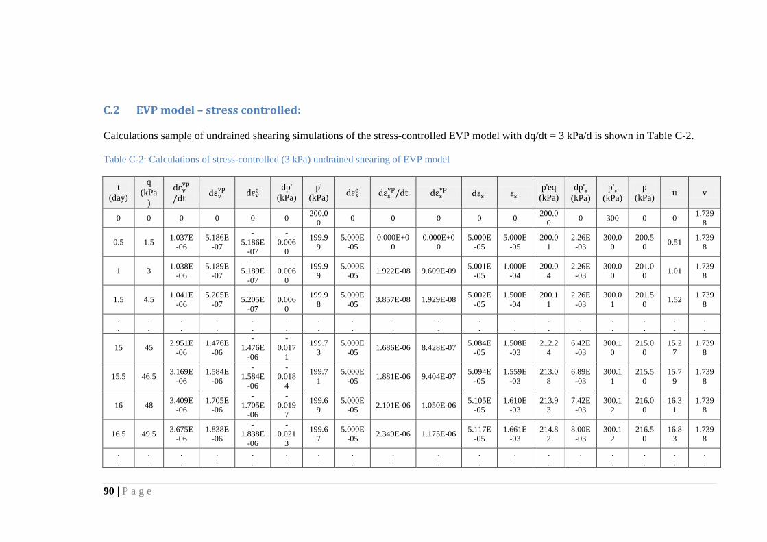
90 | P a g e
C.2 EVP model – stress controlled:
Calculations sample of undrained shearing simulations of the stress-controlled EVP model with dq/dt = 3 kPa/d is shown in Table C-2.
Table C-2: Calculations of stress-controlled (3 kPa) undrained shearing of EVP model
t (day)
q (kPa
)
dεvvp
/dt dεvvp dεve dp'
(kPa) p'
(kPa) dεse dεsvp/dt dεs
vp dεs εs p'eq
(kPa) dp'˳
(kPa) p'˳
(kPa) p
(kPa) u v
0 0 0 0 0 0 200.00 0 0 0 0 0 200.0
0 0 300 0 0 1.7398
0.5 1.5 1.037E-06
5.186E-07
-5.186E
-07
-0.006
0
199.99
5.000E-05
0.000E+00
0.000E+00
5.000E-05
5.000E-05
200.01
2.26E-03
300.00
200.50 0.51 1.739
8
1 3 1.038E-06
5.189E-07
-5.189E
-07
-0.006
0
199.99
5.000E-05 1.922E-08 9.609E-09 5.001E
-05 1.000E
-04 200.0
4 2.26E
-03 300.0
0 201.0
0 1.01 1.7398
1.5 4.5 1.041E-06
5.205E-07
-5.205E
-07
-0.006
0
199.98
5.000E-05 3.857E-08 1.929E-08 5.002E
-05 1.500E
-04 200.1
1 2.26E
-03 300.0
1 201.5
0 1.52 1.7398
.
. . .
.
. . .
.
. . .
.
. . .
.
. . .
.
. . .
.
. . .
.
. . .
.
. . .
15 45 2.951E-06
1.476E-06
-1.476E
-06
-0.017
1
199.73
5.000E-05 1.686E-06 8.428E-07 5.084E
-05 1.508E
-03 212.2
4 6.42E
-03 300.1
0 215.0
0 15.2
7 1.739
8
15.5 46.5 3.169E-06
1.584E-06
-1.584E
-06
-0.018
4
199.71
5.000E-05 1.881E-06 9.404E-07 5.094E
-05 1.559E
-03 213.0
8 6.89E
-03 300.1
1 215.5
0 15.7
9 1.739
8
16 48 3.409E-06
1.705E-06
-1.705E
-06
-0.019
7
199.69
5.000E-05 2.101E-06 1.050E-06 5.105E
-05 1.610E
-03 213.9
3 7.42E
-03 300.1
2 216.0
0 16.3
1 1.739
8
16.5 49.5 3.675E-06
1.838E-06
-1.838E
-06
-0.021
3
199.67
5.000E-05 2.349E-06 1.175E-06 5.117E
-05 1.661E
-03 214.8
2 8.00E
-03 300.1
2 216.5
0 16.8
3 1.739
8
.
. . .
.
. . .
.
. . .
.
. . .
.
. . .
.
. . .
.
. . .
.
. . .
.
. . .
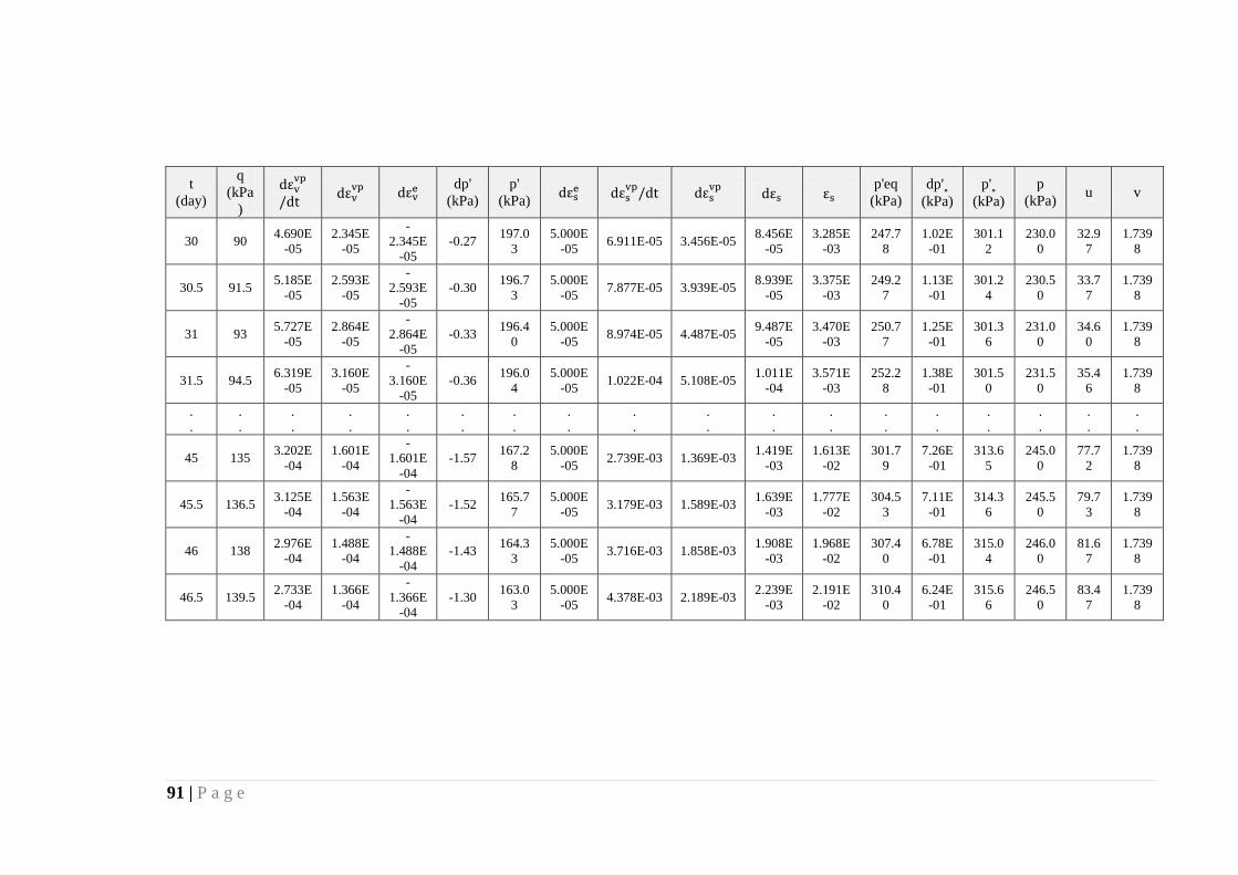
91 | P a g e
t (day)
q (kPa
)
dεvvp
/dt dεvvp dεve dp'
(kPa) p'
(kPa) dεse dεsvp/dt dεs
vp dεs εs p'eq
(kPa) dp'˳
(kPa) p'˳
(kPa) p
(kPa) u v
30 90 4.690E-05
2.345E-05
-2.345E
-05 -0.27 197.0
3 5.000E
-05 6.911E-05 3.456E-05 8.456E-05
3.285E-03
247.78
1.02E-01
301.12
230.00
32.97
1.7398
30.5 91.5 5.185E-05
2.593E-05
-2.593E
-05 -0.30 196.7
3 5.000E
-05 7.877E-05 3.939E-05 8.939E-05
3.375E-03
249.27
1.13E-01
301.24
230.50
33.77
1.7398
31 93 5.727E-05
2.864E-05
-2.864E
-05 -0.33 196.4
0 5.000E
-05 8.974E-05 4.487E-05 9.487E-05
3.470E-03
250.77
1.25E-01
301.36
231.00
34.60
1.7398
31.5 94.5 6.319E-05
3.160E-05
-3.160E
-05 -0.36 196.0
4 5.000E
-05 1.022E-04 5.108E-05 1.011E-04
3.571E-03
252.28
1.38E-01
301.50
231.50
35.46
1.7398
.
. . .
.
. . .
.
. . .
.
. . .
.
. . .
.
. . .
.
. . .
.
. . .
.
. . .
45 135 3.202E-04
1.601E-04
-1.601E
-04 -1.57 167.2
8 5.000E
-05 2.739E-03 1.369E-03 1.419E-03
1.613E-02
301.79
7.26E-01
313.65
245.00
77.72
1.7398
45.5 136.5 3.125E-04
1.563E-04
-1.563E
-04 -1.52 165.7
7 5.000E
-05 3.179E-03 1.589E-03 1.639E-03
1.777E-02
304.53
7.11E-01
314.36
245.50
79.73
1.7398
46 138 2.976E-04
1.488E-04
-1.488E
-04 -1.43 164.3
3 5.000E
-05 3.716E-03 1.858E-03 1.908E-03
1.968E-02
307.40
6.78E-01
315.04
246.00
81.67
1.7398
46.5 139.5 2.733E-04
1.366E-04
-1.366E
-04 -1.30 163.0
3 5.000E
-05 4.378E-03 2.189E-03 2.239E-03
2.191E-02
310.40
6.24E-01
315.66
246.50
83.47
1.7398

92 | P a g e
C.3 EVP model – strain controlled:
Calculations sample of undrained shearing simulations of the strain-controlled EVP model with dεs/dt = 0.3 /d is shown in Table C-3.
Table C-3: Calculations of strain-controlled (0.3 /d) undrained shearing of EVP model
t (day)
q (kPa)
dεvvp
/dt dεvvp dεve dp'
(kPa) p'
(kPa) dεse dεsvp
/dt dεsvp dεs εs p'eq
(kPa) dp'˳
(kPa) p'˳ (kPa) p (kPa) u v
0 0 0 0 0 0 0 0 0 0 0 200 200 0 300 0.00 0.00 1.7398
0.001 0.0003 0 0 3.000E
-04 9.0000
0 9.000 1.037E-06
1.037E-09
-1.037E
-09
-1.20E
-05
199.99999
200.500
4.51E-06
300.00000
203.00 3.00 1.739
8
0.002 0.0006
1.211E-07
1.211E-10
3.000E-04
9.00000 18.000 1.088E
-06 1.088E
-09
-1.088E
-09
-1.26E
-05
199.99998
202.000
4.73E-06
300.00001
206.00 6.00 1.739
8
0.003 0.0009
2.812E-07
2.812E-10
3.000E-04
8.99999 27.000 1.253E
-06 1.253E
-09
-1.253E
-09
-1.45E
-05
199.99996
204.500
5.45E-06
300.00001
209.00 9.00 1.739
8
.
. . .
.
. . .
.
. . .
.
. . .
.
. . .
.
. . .
.
. . .
.
. . .
.
. . .
0.4 0.12 3.000E-01
3.000E-04
1.189E-09
3.57E-05
165.585
1.918E-05
1.918E-08
-1.918E
-08
-2.05E
-04 183.996 367.96
6 8.52E
-05 306.318 255.19
71.20
1.7398
0.401 0.1203
3.000E-01
3.000E-04
1.167E-09
3.50E-05
165.585
1.882E-05
1.882E-08
-1.882E
-08
-2.01E
-04 183.996 367.96
6 8.36E
-05 306.318 255.19
71.20
1.7398
0.402 0.1206
3.000E-01
3.000E-04
1.145E-09
3.44E-05
165.585
1.847E-05
1.847E-08
-1.847E
-08
-1.97E
-04 183.995 367.96
6 8.20E
-05 306.318 255.19
71.20
1.7398
0.403 0.1209
3.000E-01
3.000E-04
1.124E-09
3.37E-05
165.585
1.812E-05
1.812E-08
-1.812E
-08
-1.93E
-04 183.995 367.96
6 8.05E
-05 306.318 255.19
71.20
1.7398
.
. . .
.
. . .
.
. . .
.
. . .
.
. . .
.
. . .
.
. . .
.
. . .
.
. . .

93 | P a g e
t (day)
q (kPa)
dεvvp
/dt dεvvp dεve dp'
(kPa) p'
(kPa) dεse dεsvp
/dt dεsvp dεs εs
p'eq (kPa)
dp'˳ (kPa) p'˳ (kPa) p
(kPa) u v
0.8 0.24 3.000E-01
3.000E-04
6.273E-13
1.88E-08
165.587
1.012E-08
1.012E-11
-1.012E
-11
-1.08E
-07 183.985 367.97
0 4.49E
-08 306.322 255.20
71.21
1.7398
0.801 0.2403
3.000E-01
3.000E-04
6.156E-13
1.85E-08
165.587
9.932E-09
9.932E-12
-9.932E
-12
-1.06E
-07 183.985 367.97
0 4.41E
-08 306.322 255.20
71.21
1.7398
0.802 0.2406
3.000E-01
3.000E-04
6.041E-13
1.81E-08
165.587
9.746E-09
9.746E-12
-9.746E
-12
-1.04E
-07 183.985 367.97
0 4.33E
-08 306.322 255.20
71.21
1.7398
0.803 0.2409
3.000E-01
3.000E-04
5.928E-13
1.78E-08
165.587
9.564E-09
9.564E-12
-9.564E
-12
-1.02E
-07 183.985 367.97
0 4.25E
-08 306.322 255.20
71.21
1.7398
.
. . .
.
. . .
.
. . .
.
. . .
.
. . .
.
. . .
.
. . .
.
. . .
.
. . .
1.2 0.36 3.000E-01
3.000E-04
3.300E-16
9.90E-12
165.587
5.342E-12
5.342E-15
-5.342E
-15
-5.70E
-11 183.985 367.97
0 2.37E
-11 306.322 255.20
71.21
1.7398
1.201 0.3603
3.000E-01
3.000E-04
3.244E-16
9.73E-12
165.587
5.242E-12
5.242E-15
-5.242E
-15
-5.59E
-11 183.985 367.97
0 2.33E
-11 306.322 255.20
71.21
1.7398
1.202 0.3606
3.000E-01
3.000E-04
3.202E-16
9.60E-12
165.587
5.144E-12
5.144E-15
-5.144E
-15
-5.49E
-11 183.985 367.97
0 2.28E
-11 306.322 255.20
71.21
1.7398
1.203 0.3609
3.000E-01
3.000E-04
3.128E-16
9.38E-12
165.587
5.048E-12
5.048E-15
-5.048E
-15
-5.39E
-11 183.985 367.97
0 2.24E
-11 306.322 255.20
71.21
1.7398