1

Modelling Association Football (Soccer) Results

Using the Wisdom of Crowds

- A Research on the Impact of Starting Line-ups and Player Position

Mingchuan WANG

355668

Erasmus Universiteit Rotterdam

July 2015

Abstract

“Football is round” is a commonly mentioned cliché that describes the fickle nature of the game. However,

the high level of randomness doesn’t seem to stop statisticians and econometricians from attempting to model

and predict game results. Peeters (2014) demonstrates that models utilizing crowds-assessed player “market”

valuations as inputs can produce a fairly good performance in modelling football game results. In this paper,

I attempt to improve his baseline model by further implementing the information of matchday line-ups and

player position. Even though the additional information doesn’t seem to improve model performance, the

new models are still able to yield accurate predictionsi. Meanwhile, some interesting patterns regarding

(national) team structure and player valuation are revealed during the research.

Key words: association football (soccer), starting-XI, player position, wisdom of the crowds, OLS

regression analysis.

i As I will point out later in the paper, both Peeters’ (2014) and my models are not forecasting models (they are unable to

predict the results ex ante) due to the fact that we use all the information in the modelling process.

2

1. Introduction

From a mathematical point of view, association football (soccer) can be seen as a combination of skill

and chance (Reep & Benjamin, 1968; Hill, 1973). The skill aspect of the game is represented by a

team/individual’s ability to manipulate the ball: tackling, passing, scoring, etc. The chance aspect is

represented by the randomness of football games: “purple patches”, underdogs beating favourites,

extraordinary comebacks, etc. From a fan’s perspective, it is fair to say that people enjoy the chance

part of the game as much as skills.

Statisticians and econometricians are dedicated to find the relationship between the two aspects of the

game by constructing statistical models. The most common thing to do is to model the game results

(either ex ante or ex post). Throughout the years, researchers have developed various approaches to

model football results, these models are then refined and improved. However, until recently, most of

the researches use (past) game results as the major input in computing the parameters indicating team

characteristics.

Peeters (2014) provides a new angel regarding the quality of a team. Since a football team can be broken

down into individual players, and the games are ultimately played by these players, the (aggregate)

quality of the players, measured by transfer market valuation, could be an alternative source of

information on team quality. The valuations of the players are assessed by a large pool of non-expert

internet users, each valuation can be regarded as an equilibrium price of this newly emerged “prediction

market”, a product of wisdom of the crowds. According to various researches, when the pool of

participants is sufficiently large and diverse, wisdom of the crowds is able to produce accurate

predictions (Wolfers and Zitzewitz, 2004; Wolfers and Zitzewitz, 2007). Results from Peeters (2014)

confirms the theory of wisdom of crowds. It seems that the consolidated valuation of players by internet

users provides a quite precise representation of player quality. Models using these valuations as inputs

are able to outperform models implied by bookmakers’ odds on a significant margin.

The success of Peeters’ model implies: 1. the valuation of the players are rather accurate (or systematic

errors are successfully averted by choosing international games instead of club games); 2. A model

using player valuation could provide more information (or perhaps less noise) than that using game

3

results.

This paper is an attempt to refine the models suggested by Peeters (2014) by adding matchday roster

information (starting line-up, substitutes) and player position information (GK/DF/MF/FW) into

consideration. The models in Peeters (2014) use standard ordered probit approach to model match

results directly, this paper will be attempting a slightly different approach, to model goal differencesii

and then deduce the results from the predicted goal differences.

Due to the rules of football games, not all players on the team roster will participate directly in a match.

For each game, a significant proportion of the players will be benched and won’t be having any playing

time at all. It is logical to think that the starting-eleven, along with the players who came in from the

bench, would have more influence on the game results than those who haven’t played. Under this

assumption, models using the player valuations of the starting-eleven (and substitutes) could in theory

outperform models using the valuation of the whole team.

In practice, my regression analyses show that the additional information of starting line-up doesn’t

significantly improve the models, while the additional information of the valuation of substitutes would

slightly deteriorated their performance. Nonetheless, the starting-eleven-model can be regard as a good

alternative to the whole-team-model in terms of prediction accuracy, however neither model is superior

to the other.

On top of that, another player-level factor that could affect the game results could be player position.

Modern football is a highly tactical and well organised sport, in general the players are categorised into

goalkeepers, defenders, midfielders, and forwards based on their roles and positions on the pitch.

Players on different positions have different playing styles, and contribute differently to the game. I

suspect that dissecting team valuations into more detailed “position based valuations” would produce a

more accurate description on team quality, and thus lead to better model performance.

ii In football, goal difference equals to the total amount of goals scored minus the total amount of goals conceded by a team in

a certain period (usually a season or a cup tournament). Goal difference in this paper refers to the difference between goals

scored and conceded in one specific game. It can also be referred to as “match goal difference”, or “winning margin” in betting.

4

Results indicate that the additional information of player position does not significantly improve the

performance of the models. However, it does reveal some interesting pattern in player contribution and

valuation. For instance, it appears that attackers are in general overvalued and defenders are

systematically undervalued.

In Section 2 I will present the related literatures concerning football forecasting (modelling), wisdom

of the crowd, and other related topics. In Section 3 I will present the concept of modelling goal

difference. Section 4 gives a short description on the data I will be using in this paper. In Section 5 I

will propose a set of goal difference oriented models based on player valuation and match day line-ups.

I will then compare the performance of these models along with the bookmakers’ odds. In Section 6 I

will further incorporate the information of player position in to my models. The performance of these

models will be evaluated. I will conclude the research in the last section.

2. Literature review

Stekler, et al. (2010) discuss several issues in sport forecasting. The authors classify sport forecasting

into three categories: 1. Betting market forecasting, which bookmakers’ odds can be interpret as forecast

probabilities; 2. Modelling, which involves the use of statistical models and other mathematical means

to compute the probabilities of scores or results; 3. Experts, which include the opinions of individuals

such as pundits, journalists, commentators who may or may not reveal their means of forecasting.

When it comes to forecasting football results, various researches have shown that the experts’ opinions

such as those of newspaper tipsters has little value (Forrest & Simmons, 2000; Pope & Peel, 1989).

The bookmakers’ odds, on the other hand, are generally believed to have a good predictive accuracy

(Boulier & Stekler, 2003; Forrest, Goddard, & Simmons, 2005). There exists evidence that the

bookmakers’ odds can sometimes be biased, for instance, the favourite-longshot bias (Cain, Law, &

Peel, 2000), however the scale of the biases should be rather small, since heavy deviation from the real

odds would put the bookmakers themselves in significant risk. The reason behind an accurate

bookmakers’ odds is simple: in theory, bookmakers make their living in the betting market, they have

to be efficient in incorporating all possible information in order to survive. If a bookmaker could be

5

systematically beaten, he would simply cease to operate in the market. For this reason, bookmaker’s

odds are thus used as reference points and benchmark models by statisticians and economists when

modelling football game results. Examples can be found in the researches of Hvattuma and Arntzenb

(2010), and Peeters (2014). In this paper, bookmakers’ odds will be used to serve the same purpose.

In previous literatures, modelling match results in association football is usually done in two means.

The first approach, which is favoured by most applied statisticians, models the number of goals scored

and conceded, the match result (win/draw/loss) can then be derived from the goal difference. The goal-

oriented approach usually involves the use of univariate and bivariate Poisson distribution with

(dynamic) parameters representing the attacking and defensive qualities of the teams. Maher (1982)

was one of the first researches that attempted to model football in this way, however, his model was

incapable of forecasting. Dixon and Coles (1997) proposed an improved model with forecasting

capabilities. Dynamic attacking/defence parameters are later introduced into the models by the likes of

Rue and Salvesen (2000) and Crowder, et al. (2002).

An alternative approach is favoured by a number of applied econometricians, the method is to model

the win/draw/loss results directly with discrete choice regression models such as ordered probit and

logit analysis. Such approach is used by the likes of Goddard and Asimakopoulos (2004); Cain, Law,

and Peel (2000); Dixon and Pope (2004); and Peeters (2014).

Goddard (2005) attempted to compare the forecasting performance of the two approaches by comparing

the performance of different models (goal-oriented, result-oriented and hybrids) using a data set of 25

years of English league football results. By using the pseudo-likelihood statistic suggested by Rue and

Salvesen (2000) as the measure of the forecasting performance, Goddard (2005) concludes that there

are little difference between the two approaches in terms of forecasting performance. It is not a

surprising result since the two methods are just different interpretations of the same information. In fact,

most literatures mentioned so far regarding football result modelling (whether directly or through goal

difference) mainly operates on a similar type of information, namely the game results that the team

played.

6

In contrast with the conventional approaches, Peeters (2014) takes a different path. Instead of using

goals scored/conceded in the (previous) games, Peeters (2014) uses the market value of players as the

measurement of the quality of the team. The information of the player valuation was obtained from the

public website Transfermarkt.de, these valuations can be regarded as the collective wisdom of

thousands of users of the website.

Researches on the wisdom of crowds and prediction markets (such as Wolfers and Zitzewitz, 2004;

Wolfers and Zitzewitz, 2007; Golub and Jackson, 2011) suggest that with a large and diversified group,

the outcome of the prediction market can outperform the prediction of a small group of experts (in this

case, the bookmakers). As a result, an ordered probit model based on player valuation can outperform

the probability indicated by bookmakers’ odds on international football results (Peeters, 2014).

3. Modelling match goal difference

A football match between team i and j at time t can produce no more than three outcomes, therefore,

the game result 𝑦𝑖𝑗𝑡 is a categorical variable that takes three values, a win/draw/loss for team i.

According to Peeters & Szymanski (2014), and Peeters (2014), 𝑦𝑖𝑗𝑡∗ , an unobservable continuous

equivalent of 𝑦𝑖𝑗𝑡, can be described as:

𝑦𝑖𝑗𝑡∗ =

𝜃𝑖𝑡∏𝑞𝑎𝑖𝑡𝛽𝑎

𝜃𝑗𝑡∏𝑞𝑎𝑗𝑡𝛽𝑎

exp(𝜀𝑖𝑗𝑡) (1)

In equation (1), 𝑦𝑖𝑗𝑡∗ has two estimated threshold −𝛾 and 𝛾. When 𝑦𝑖𝑗𝑡

∗ ≤ −𝛾, the model records a

loss for team i; when −𝛾 < 𝑦𝑖𝑗𝑡∗ ≤ 𝛾, the model predicts a draw between the two teams; and when

𝑦𝑖𝑗𝑡∗ > 𝛾, the model implies a win for team i. On the other side of the equation, q represents the

characteristics of the respective teams, each characteristic q has an exponential parameter 𝛽 which

describes its relative level. Furthermore, 𝜃 represents the effect of home advantage, the noise term 𝜀

represents the chance factors, both phenomenon are generally believed to be present in most modern

football games. Taking the logarithms of the characteristic parameters will lead to:

𝑦𝑖𝑗𝑡∗ = log(𝜃𝑖𝑡) − log(𝜃𝑗𝑡) + ∑ 𝛽𝑎 log(𝑞𝑎𝑖𝑡)𝑎 −∑ 𝛽𝑎 log(𝑞𝑎𝑗𝑡)𝑎 + 𝜀𝑖𝑗𝑡 (2)

A standard ordered probit procedure can then applied to recover the parameters.

Other than a win/draw/loss, the result of a football game can also be reported as goal difference. The

7

goal difference 𝑚𝑖𝑗𝑡 of a game at time t, is calculated as the number of goals scored minus number of

goals conceded by team i. It can be easily translate into win/draw/loss result: a positive goal difference

implies a win, a negative one implies a loss, and a nil represents a draw. Goal differences also provides

a better knowledge on the “strength” of the two sides: a narrow 2-1 win is indifferent with a 7-1 drubbing

in a win/draw/loss system. Therefore, the model developed by Peeters & Szymanski (2014) can in

theory be used to model goal difference as well, the recovered parameters could even be more accurate.

Similar to equation (2) we can have:

𝑚𝑖𝑗𝑡 = 𝑚𝑖𝑗𝑡∗ = 𝜃 𝑑𝑖𝑡 + ∑ 𝛽𝑎 log(𝑞𝑎𝑖𝑡)𝑎 + ∑ 𝛽𝑎 log(𝑞𝑎𝑗𝑡)𝑎 + 𝜀𝑖𝑗𝑡 (3)

In equation (3), 𝑚𝑖𝑗𝑡∗ is the unobservable continuous equivalent of 𝑚𝑖𝑗𝑡, 𝜃 measures the effect of

home advantage, 𝑑𝑖𝑡 is a dummy variable which takes the value “1” when the nominal home team,

team i, has real home advantage.

The parameters of equation (3) can be estimated by ordinary least squares (OLS) regression and then

the predicted values of 𝑚𝑖𝑗𝑡∗ can be calculated. The odds of a win/draw/loss can then be computed

using an ordered probit procedure with game result 𝑦𝑖𝑗𝑡 as the dependent variable and the predicted

𝑚𝑖𝑗𝑡∗ values as the only independent variable.

4. Data

The data used in this paper are the same ones that were used in Peeters (2014) except a few additional

entries. It records a total of 1048 non-friendly international games happened during the 2008-2014

period. Amongst which, 806 games were played between European national teams (members of The

Union of European Football Associations, UEFA), including the European qualifier games for the FIFA

World Cup 2010 and 2014, qualifier games for the Euro 2012, games of the Euro 2012 tournament, and

games between UEFA nations during World Cup 2010 and 2014. The remaining 242 games consist

mostly of the games played by members of the South American Football Confederation (CONMEBOL),

including the South American qualifier games for the World Cup 2010 and 2014, the games of 2011

Copa América tournament, along with games played in World Cup 2010 and 2014 involving non-UEFA

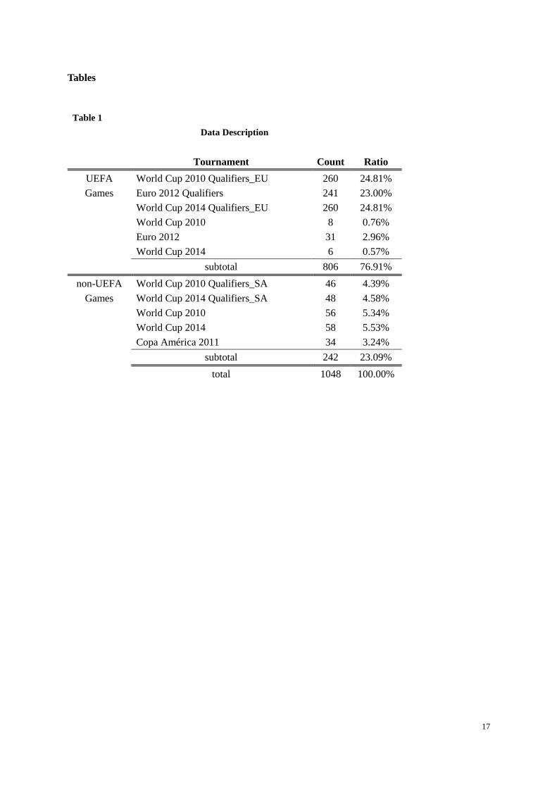
teams. Table 1 provides an overview on the data.

8

[Insert Table 1 here.]

The valuations of the players are obtained from the website Transfermarkt.de. They are the latest

“market value” posted on the website at the time of the game. The website functions as a public forum.

Football enthusiasts can post comments on the performance and market value of a specific player. In

time, the website gathers the user entries and update the market value of that player. Since the website

is used by thousands of users across Europe, Peeters (2014) suggests that it can be regarded as a source

of the wisdom of crowds. According to Simmons et al. (2011), one of the most important conditions for

crowds to produce an accurate collective assessment is that the members of the crowds should be

sufficiently large and diverse. Unfortunately, due to the fact that the website was originated from

Germany, users who affiliate in German clubs dominate the population. An overview on user club

preference published by the site on 31st.10.2013 shows that more than 70% of the users are affiliated to

a club from German 1st to 3rd division (1.Bundesliga, 2.Bundesliga, and 3.Liga), other important user

groups include the Turkish Süper Lig (6%)iii, the English Premiere League (5%), the Italian Serie A

(4%), and the Spanish Primera División (3%).

As a result, players from the popular leagues receive significantly more comments and assessments

from users than players who play elsewhere. For almost all professional footballers, the majority of the

games played are club games. Therefore, the valuations of players are assessed based mainly on their

performance in club competitions, and thus can be heavily influenced by club specific factors such as

the quality or playing style of the club manager as well as club popularity. In order to avoid the potential

club-level bias, Peeters (2014) suggests to use international games instead of club competitions as the

target of the study. A national team usually calls up players from all sorts of clubs, both popular ones

and unpopular ones; a player can change the club he played for, but his nationality is rather fixed. In

this sense, international games should provide a more unbiased platform for the study.

iii This is due to the fact that Turkish immigrants and descendants form the largest ethnic minority in Germany. As a result,

Peeters (2014) discovers that the Turkish players are in general overvalued on Transfermarkt.

9

5. Model comparison: full squad roster, starting-XI, substitutes, and bookmakers’ odds

The team roster of a national team usually contains 18 to 23 players. For a typical football game, each

side can only field 11 players initially (commonly known as the starting-eleven) and a maximum of 3

potential substitutes. Even if the manager would send on all 3 substitutes, 4 to 9 players still wouldn’t

participate at all in terms of playing. I suspect that these benched players would have much less impact

on the game result than their fielded colleagues. Furthermore, managers usually prefer to start with his

best players, these starters are generally more popular than benched players among fans, and thus

receives more discussions and assessments on the forum. Therefore, the evaluation on these popular

starters might be more accurate. Combining these two factors , it is reasonable to suspect that a model

based on the valuation of starters (and substitutes) would produce a better result than a model based on

the valuation of the whole team (as did in Peeters, 2014).

Table 2 shows the estimated results of 6 models based on equation (3). Model 1-3 operate on the full

data set of 1048 games, while Model 4-6 use a subset of 806 games when both sides featured in the

match are European teams (members of UEFA). Besides the home advantage term 𝜃, which is present

in every model, Model 1 and Model 4 use the average values (logarithms) of all player in both teams as

the quality characteristic q; in Model 2 and Model 5, q is narrowed down to the average values of the

starting-eleven from both sides; and in Model 3 and Model 6, the average values of all players involved

in the game (starting-XI plus subs) from both teams are used.

[Insert Table 2 here.]

Similar to Peeters (2014), each game is used twice during the regression analyses, one from either sides’

perspective. The reason to do so is that only few games in the data set are held on neutral grounds

(including the final tournaments of FIFA World Cups, UEFA European Championships, and Copa

América), most of the games (the qualifiers) are played with home advantage. We can see from Table 1

that 935 games out of 1048 (89%) in the full data set, and 773 out of 806 (96%) in the UEFA subset are

played on a home turf. This means that in majority of the cases, the dummy variable 𝑑𝑖 in equation (3)

takes the value “1”. As a result, the regression will “confuse” the home advantage term with the

interception, which leads to inaccurate estimate of the parameters.

10

The home advantage parameter appears to be positive and significant in all 6 models (not playing at

home results in a 0.66-0.77 deficit in goal difference), which is consistent with most existing literatures.

The estimated parameters of player valuations are also in line with those of Peeters’ (2014).

In general, models using all-game-data are outperformed by models using the UEFA-game subset in

terms of 𝑅2. The finding confirms the “diversity” assumption of the wisdom of the crowds: a significant

number of players featured in the non-UEFA games are playing for teams in unpopular leagues, and

thus receive significantly less attention from users. The lack of entries ultimately leads to an inaccurate

assessment of player valuation. Surprisingly though, the variations of 𝑅2 are rather small within

groups. In both groups, models using average values of starters (Model 2&5) have the highest 𝑅2,

followed by models using average values of the whole team (Model 1&4), models using average values

of all fielded players (Model 3&6) have the lowest 𝑅2.

Now that the parameters are successfully recovered, predicted values of 𝑚𝑖𝑗𝑡∗ can be computed by

applying equation (3). The predicted 𝑚𝑖𝑗𝑡∗ can then be translated into win/draw/loss odds using an

ordered probit procedure where the dependent variable is the match results 𝑦𝑖𝑗𝑡 and 𝑚𝑖𝑗𝑡∗ is the only

predictor. Table 3 presents the descriptive statistics of the ordered probit regressions:

[Insert Table 3 here.]

Following Frank et al. (2010), and Peeters (2014), this paper will also be using geometric mean as the

criteria to evaluate the goodness-of-fit performance of the models. Table 4 presents the results of a series

of paired t-tests between the models, the bookmakers’ odds (BM), and a null model (MN) in which the

odds of win/draw/loss are equal to the observed averageiv.

iv Out of all 1048 games, there are 484 wins, 235 draws, and 329 losses. Thus, for the Null Model, 𝑝(ℎ𝑜𝑚𝑒𝑤𝑖𝑛) =

484

1048≈

0.46, 𝑝(ℎ𝑜𝑚𝑒𝑑𝑟𝑎𝑤) =235

1048≈ 0.22, and 𝑝(ℎ𝑜𝑚𝑒𝑙𝑜𝑠𝑠) =

329

1048≈ 0.31. Similarly, the odds of win/draw/loss of the Null

Model of UEFA-games are 0.45, 0.21, and 0.34 respectively.

11

[Insert Table 4 here.]

All models outperformed the null model and bookmakers’ odds with a significant margin (𝑝 < 0.05).

Models featuring the average values of all fielded players (Model 3&6) once again have the worst

performance in their respected groups. Models using the average values of the whole team (Model 1&4)

have roughly the same prediction accuracy with models using the average values of starting-eleven

(Model 2&5).

Combining the results of Table 2 and Table 4, it can be concluded that adding the information of starting

line-ups does not significantly improve the model (meanwhile it doesn’t hurt either). On the other hand,

trying to include the information of substitutes will somehow slightly deteriorate the model. It suggests

that all (national) teams share a similar structure, the quality of the bench are in general proportionate

to the quality of starters. In other words, a good starting line-up implies a good bench, and vice versa.

In the meantime, due to the limit on player amount and playing time, the quality of the fielded substitutes

are disproportionate to the quality of the teams, and thus (slightly) hampers the performance of the

models.

6. Player position

Even though individual brilliance can sometimes decide a game, no one would disagree that modern

football is at its root a team sport. For a team to function properly, the players should be well organized

and coordinated. In modern football, each player is assigned with a specific role based on his position

on the pitch. The position of a player is so important that it becomes an inseparable part of the player’s

identity (even long after he retired)v.

A rather reductive but generally acknowledged way is to categorise football players into goalkeepers

(GK), defenders (DF), midfielders (MF), and forwards (FW). Despite the fact that the number of players

from each department varies depending on the manager’s choice of formation, some general patterns

v When the name of a football player is mentioned, it is a common practice to indicate his position as one of the most basic

information. For instance, we usually address Arjen Robben as the Dutch Winger; Rio Ferdinand as the ex-ManUtd centre

back, etc.

12

are still followed. For instance, only one goalkeeper is allowed to play on the field for either teams, the

number of defenders is at least 3 for most of the teams, and teams usually do not field more than 3

forwards… In club football, managers have the opportunities to sign players from a wide pool of

selections. The quality of players varies from team to team due to the difference in financial capabilities

between clubs, but the quality of the players within a team is usually constant. In other words, in club

football, good attackers tends to play alongside with good midfielders and good defenders, vice versa.

Team building works differently in national teams. National team managers face a narrower pool of

selection comparing to club managers. As a result, sometimes the quality of players in each department

differs within a team. It is then reasonable to suspect that the in-team variations of quality might affect

the result of a game. For instance, a team with excessive attacking talents, a weak midfield, and a poor

defence-line can be easily outplayed by a more “balanced” side with less average player value. In this

sense, adding the information of player position might improve the performance of the models.

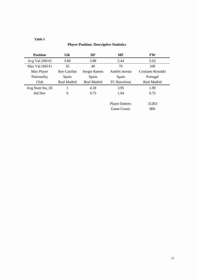
Table 5 presents the descriptive statistics regarding player positionvi, including the average player value

of each position, the information of the most valuable player on each position, along with the average

number and standard deviation of starters for each position. According to the table, it seems that as we

move up-field towards the opponent’s goal, the number of players drops, and the average value of the

players rises.

[Insert Table 5 here.]

Based on Model 5, three more models are developed to investigate the effect of player position on game

results. As it shows in Table 6, Model 7 employs the average value of each position as separate quality

parameters in the regression, in Model 8 the value of the most valuable player in each department is

applied as q, and in Model 9 both the average and maximum values are implemented.

vi The information on player position in the non-UEFA games are not complete, thus Model 7-9 are based on the subset of

806 UEFA games. Note that the goalkeepers and defenders are clustered into the same category (DFGK) in these 3 models.

13

[Insert Table 6 here.]

Some of the estimated parameters of Model 9 are neither correct nor significant, apparently it cannot

be considered as a valid model. Both Model 7 and 8 outperformed the null model as well as the

bookmakers’ odds on a significant margin (𝑝 < 0.05), yet none of the two models can beat Model 5

either in terms of data fitness (𝑅2) or predictive accuracy (geometric mean).

In spite of not being able to improve model performance, Model 7 and 8 do reveal some interesting

patterns. In both models, as we move from defence to offence, the estimated 𝛽 decrease drastically. In

Model 7, where we use the average prices of each position as covariates, 𝛽 of defence (including

defenders and goalkeeper) are higher than 0.6; as we move to the midfield, 𝛽 drop to round 0.3; and

for forwards, the estimated 𝛽 are lower than 0.1. When we use the maximum instead of average values

as covariates, the estimated 𝛽 follow a similar trend, in Model 8 the respective 𝛽 for each department

are around 0.5, 0.3, and 0.1. It seems that there exists a significant gap between the “contributions per

unit market value” of each departments. In other words, defenders are undervalued and attackers are

overvalued in terms of their contribution to goal difference. The result further implies that, in a match

where the two sides have the same average quality, the side with better defence would have a much

better chance in winning the game.

Unfortunately, few literatures can be found on explaining this phenomenon. Based on my knowledge

about football, I propose the following reasons: 1. Due to the nature of their roles, attacking players

mainly operates on the ball while defensive players are usually off the ball. Therefore, it is in general

easier to evaluate the performance of attackers than defenders. For forwards and attacking midfielders,

parameters such as goals scored, assists, number of passes, and passing accuracy can provide a good

assessment on player quality. For defensive players however, few stats can visualize their involvements

correctlyvii, and thus leads to a systematic undervalue on their contributions. 2. No football games can

be won merely by defending. From a defensive perspective, the best result of a game is to keep a clean

vii Player-level defensive stats such as tackles, interceptions, duals won, etc. are heavily reliant on team-level characteristics.

For instance, the lack of tackles and interceptions doesn’t necessarily mean a defender is bad at defending, it can be a simple

result of lack of attacking from the opposite team.

14

sheet (no goals conceded). Though keeping a clean sheet is never enough to ensure a victory, a team

still have to score to win. On the other hand, from an attacking perspective, a team can always win by

scoring more goals than the opponent. In this sense, attacking players are considered to be potential

match “deciders” and thus more valuable than their defensive colleagues. 3. Attacking players,

especially the best attackers, are in general more popular than defenders among fans, and thus have

higher commercial value. Such phenomenon is called “Superstar Effects”. According to a research

based on Italian football by Lucifora and Simmons (2003), the marginal revenue (the extra price a

spectator willing to pay to see the player play) generated by a “top player” is significantly higher than

the rest of the players. Most of these top players are either forwards or attacking midfielders.

One last point worth mentioning concerns Model 8. Amongst all the models I built in this paper, Model

8 requires the least amount of information while is still able to produce a fairly good result. It seems

that by applying the theory of wisdom of crowds, a model based on the information of as few as 6

players (3 from each side) is sufficient enough to beat the bookmakers’ odds.

7. Conclusion

In this paper I attempt to improve the baseline model proposed by Peeters (2014) by including additional

information of starting line-ups and player positions. Instead of modelling game results (win/draw/loss)

directly, models in this paper use match goal difference as an alternate dependent variable. The predicted

goal difference are then used to deduce the odds of a win/draw/loss. The results confirms the findings

of Peeters (2014): the non-expert opinions of internet users seem to produce a fairly accurate assessment

on player market value, a model based these valuations can outperform bookmakers’ odds. The theory

of wisdom of crowds further implies that more user entries would lead to better assessment, as a result,

models based on a more popular UEFA-games subset produce better performance.

Using the average value of starting line-ups (instead of the whole team) as the quality parameters

couldn’t significantly improve the performance of the models as I initially expected. One possible

explanation could be the similarities in team structure, that the quality of bench is always proportionate

to the qualities of starters. Adding the value of substitutes into the models consequently deteriorate the

performance (slightly). It seems that the quality of substitutes in not a good representation of team

15

quality. It is not much of a problem if the ultimate goal is to predict game results, since it is impossible

to know the substitutions before the game anyway.

Classifying players according to their positions couldn’t significantly improve the performance of the

models either. Though some interesting patterns are unveiled in the process. According to my results,

there exists a systematic overvalue on the market value of attackers and undervalue on defenders in

terms of contribution to goal difference per unit market value. I suspect it is due to three reasons: 1. It

is more difficult to assess the contribution of defensive players; 2. No matter how good the defence is,

a team still need to score to win, and thus attackers are more “important” than defenders; and 3. (Good)

attacking players generate significant more marginal revenue than the rest of the team due to the

superstar effects. Results on player position also indicate that a model based on the value of as few as

6 players (the best player in each department, 3 from each side) is sufficient enough to beat the

bookmakers’ odds.

There are two major limitation regarding this paper. Similar to Peeters (2014), the models in this paper

use all the games in the estimation process, and thus are incapable of producing predictions ex ante.

The second limitation concerns the data. So far the crowd wisdom models can only be applied to

international games due to potential user bias on the club/league-level. However, with the growth of the

website, the user pool will be larger and more diversified. It is reasonable to suspect that a similar model

could be used to model and even forecast club football results in the foreseeable future.

References

Peeters, Thomas. (2014). Testing the wisdom of crowds: transfermarkt valuations and international football

results (preliminary version). Erasmus University Rotterdam.

Boulier, B.L., & Stekler, H.O. (2003). Predicting the outcomes of National Football League games.

International Journal of Forecasting 19, 257–270.

Cain, M., Law D., & Peel, D. (2000). The favourite-longshot bias and market efficiency in UK football

betting. Scottish Journal of Political Economy, 47, 25–36.

16

Crowder, M., Dixon, M., Ledford, A., & Robinson, M. (2002). Dynamic modelling and prediction of English

Football League matches for betting. Statistician, 51, 157–168.

Dixon, M.J., & Pope, P.E., (2004). Modelling association football scores and inefficiencies in the football

betting market. Applied Statistics 46, 265-280.

Forrest, D., & Simmons, R., (2000). Forecasting sport: the behaviour and performance of football tipsters.

International Journal of Forecasting 16, 317–331.

Forrest, D., Goddard, J., & Simmons, R. (2005). Odds-setters as forecasters: the case of English football.

International Journal of Forecasting 21, 551–564.

Golub, B., & Jackson, M. O. (2010). Naïve Learning in Social Networks and the Wisdom of Crowds.

American Economic Journal: Microeconomics, 2(1), 112-149.

Goddard, J., & Asimakopoulos, I., (2004). Forecasting football results and the efficiency of fixed-odds

betting. Journal of Forecasting Volume 23, Issue 1, 51–66.

Goddard, John. (2005). Regression models for forecasting goals and match results in association football.

International Journal of Forecasting 21, 331– 340.

Hvattuma, M.L., & Arntzenb, H. (2010). Using ELO ratings for match result prediction in association

football. International Journal of Forecasting 26, 460–470.

Lucifora, C., & Simmons, R. (2003). Journal of Sports Economics February 2003 vol. 4 no. 1, 35-55.

Maher, J.M. (1982). Modelling association football scores. Statistica Neerlandica, 36, 109– 118.

Pope, P.F., & PEEL, D.A. (1989). Information, Prices and Efficiency in a Fixed-Odds Betting Market.

Economica. New Series, Vol. 56, No. 223, 323-341

Reep, C., & Benjamin, B. (1968). Skill and Chance in Association Football. Journal of the Royal Statistical

Society. Series A (General), Vol. 131, No. 4, 581-585.

Rue, H., & Salvesen, O. (2000). Prediction and retrospective analysis of soccer matches in a league. .

Statistician, 49, 399– 418.

Stekler, H.O., Sendor, D., & Verlander, R. (2010). Issues in sports forecasting. International Journal of

Forecasting 26, 606–621.

Wolfers, J., & Zitzewitz, E. (2004). Prediction Markets. The Journal of Economic Perspectives, 18, 107-126.

Wolfers, J., & Zitzewitz, E. (2007). Interpreting Prediction Market Prices as Probabilities. National Bureau

of Economic Research Working paper 12200.

17

Tables

Table 1

Data Description

Tournament Count Ratio

UEFA World Cup 2010 Qualifiers_EU 260 24.81%

Games Euro 2012 Qualifiers 241 23.00%

World Cup 2014 Qualifiers_EU 260 24.81%

World Cup 2010 8 0.76%

Euro 2012 31 2.96%

World Cup 2014 6 0.57%

subtotal 806 76.91%

non-UEFA World Cup 2010 Qualifiers_SA 46 4.39%

Games World Cup 2014 Qualifiers_SA 48 4.58%

World Cup 2010 56 5.34%

World Cup 2014 58 5.53%

Copa América 2011 34 3.24%

subtotal 242 23.09%

total 1048 100.00%

18

Table 2 Descriptive Statistics, Model 1-6

Model Covariates B Std Err Sig R^2

All 1 HomeReal -0.767 0.071 0.000 0.472 HomeReal

Games LogAvg_H_All 1.333 0.045 0.000 0 1161

LogAvg_A_All -1.276 0.045 0.000 1 935

2 HomeReal -0.754 0.071 0.000 0.476 Total 2096

LogAvg_H_Sta 1.330 0.044 0.000

LogAvg_A_Sta -1.275 0.044 0.000

3 HomeReal -0.765 0.072 0.000 0.468

LogAvg_H_Pla 1.329 0.045 0.000

LogAvg_A_Pla -1.271 0.045 0.000

UEFA 4 HomeReal -0.675 0.080 0.000 0.523 HomeReal

Games LogAvg_H_All 1.342 0.047 0.000 0 839

LogAvg_A_All -1.311 0.047 0.000 1 773

5 HomeReal -0.659 0.079 0.000 0.529 Total 1612

LogAvg_H_Sta 1.341 0.046 0.000

LogAvg_A_Sta -1.311 0.046 0.000

6 HomeReal -0.674 0.080 0.000 0.520

LogAvg_H_Pla 1.340 0.047 0.000

LogAvg_A_Pla -1.309 0.047 0.000

19

Table 3

Ordered Probit Regressions: Estimated Results

Model 1 2 3 4 5 6

Coefficient 0.785 0.790 0.782 0.859 0.867 0.856

Sig. 0.000 0.000 0.000 0.000 0.000 0.000

Log Likelihood -1705.71 -1708.44 -1711.83 -1178.48 -1179.96 -1183.08

Pseudo R^2 0.239 0.238 0.237 0.310 0.310 0.308

Model 5 7 8

Coefficient 0.867 0.940 0.936

Sig. 0.000 0.000 0.000

Log Likelihood -1179.96 -1235.21 -1252.15

Pseudo R^2 0.310 0.277 0.266

20

Table 4

T-tests on geometric means M1-6

Models Mean Std Dev Sig

All MN-M1 -0.1599 0.2306 0.0000

Games MN-M2 -0.1599 0.2307 0.0000

MN-M3 -0.1589 0.2210 0.0000

BM-M1 -0.0118 0.0849 0.0000

BM-M2 -0.0118 0.0917 0.0000

BM-M3 -0.0106 0.0876 0.0000

M1-M2 0.0000 0.0284 0.9626

M1-M3 0.0012 0.0186 0.0030

UEFA MN-M4 -0.1992 0.2449 0.0000

Games MN-M5 -0.1988 0.2445 0.0000

MN-M6 -0.1979 0.2440 0.0000

BM-M4 -0.0259 0.0847 0.0000

BM-M5 -0.0255 0.0913 0.0000

BM-M6 -0.0247 0.0873 0.0000

M4-M5 0.0004 0.0277 0.5787

M4-M6 0.0013 0.0182 0.0047

21

Table 5

Player Position: Descriptive Statistics

Position GK DF MF FW

Avg Val (Mil €) 3.60 3.88 5.44 5.62

Max Val (Mil €) 35 40 70 100

Max Player Iker Casillas Sergio Ramos Andrés Iniesta Cristiano Ronaldo

Nationality Spain Spain Spain Portugal

Club Real Madrid Real Madrid FC Barcelona Real Madrid

Avg Num Sta_XI 1 4.18 3.95 1.90

Std Dev 0 0.75 1.04 0.75

Player Entries: 31263

Game Count: 806

22

Table6

Model comparison: 7-9

geometric mean

Model Covariates B

Std

Err Sig Adj R2 >Null >BM >M5

7 HomeReal -0.662 0.080 0.000 0.516 Y Y N

LogAvg_Home_DFGK 0.648 0.069 0.000

LogAvg_Away_DFGK -0.629 0.069 0.000

LogAvg_Home_MF 0.301 0.049 0.000

LogAvg_Away_MF -0.299 0.049 0.000

LogAvg_Home_FW 0.089 0.028 0.010

LogAvg_Away_FW -0.088 0.028 0.020

8 HomeReal -0.671 0.082 0.000 0.501 Y Y N

LogMax_Home_DFGK 0.554 0.061 0.000

LogMax_Away_DFGK -0.541 0.061 0.000

LogMax_Home_MF 0.329 0.043 0.000

LogMax_Away_MF -0.324 0.043 0.000

LogMax_Home_FW 0.125 0.027 0.000

LogMax_Away_FW -0.123 0.027 0.000

9 HomeReal -0.659 0.080 0.000 0.524

LogAvg_Home_DFGK 1.901 0.341 0.000

LogAvg_Away_DFGK -1.745 0.342 0.000

LogAvg_Home_MF 0.528 0.330 0.110

LogAvg_Away_MF -0.477 0.330 0.149

LogAvg_Home_FW -0.144 0.351 0.681

LogAvg_Away_FW 0.139 0.351 0.692

LogMax_Home_DFGK -1.173 0.306 0.000

LogMax_Away_DFGK 1.043 0.306 0.001

LogMax_Home_MF -0.270 0.301 0.370

LogMax_Away_MF 0.216 0.301 0.473

LogMax_Home_FW 0.189 0.340 0.579

LogMax_Away_FW -0.187 0.340 0.583