Modelling and Stability Analysis of Power Systems with...

Modelling and Stability Analysis of Power Systems

with inclusion of Delays

Prof. Federico Milano

Email: [email protected]

Webpage: faraday1.ucd.ie

School of Electrical & Electronic Engineering

University College Dublin

Dublin, Ireland

Sevilla, May 16th, 2016 Modelling and Stability Analysis of Power Systems with inclusion of Delays - 1

Biography

• Federico Milano received from the University of Genoa, Italy, the Electrical Engineering

degree and the Ph.D. degree in 1999 and 2003, respectively.

• In 2001 and 2002, he worked at the University of Waterloo, Canada, as a Visiting

Scholar.

• From 2003 to 2013, he was with University of Castilla-La Mancha, Ciudad Real, Spain.

• He joined University College Dublin, Ireland, in 2013, where he is currently Professor

of Power System Control and Protections.

• In 2016, he has been elevated to IEEE Fellow for his contributions to power system

modelling and simulation.


Contents

• Functional differential equations

• Small-signal stability of standard DAE

• Small-signal stability of delayed DAE

• Numerical Libraries for Eigenvalue Analysis

• How do delays affect system stability?


Functional Differential Equations

Sevilla, May 16th, 2016 Functional Differential Equations - 1

Differential Algebraic Equations

• The most general form of DAEs is:

Φ(z, z, t) = 0 (1)

where t is the time, z(t) ∈ Rn is the state vector, and z = dz/dt is the state

derivative.

• It is assumed that Φ(z, z, t) is continuously differentiable with respect to all its

arguments.

• The system (1) is sometimes called Implicit Differential Equations (IDEs).

• Clearly, (1) includes Ordinary Differential Equations (ODEs):

Φ(z, z, t) = z − F (z, t) = 0 (2)


Hessenberg Index-1 Form

• In power system analysis, z are split into state variables x and algebraic variables y

(y = 0) so that (1) can be written explicitly as coupled differential and algebraic

equations.

• In particular, the Hessenberg Index-1 Form is the standard model used for transient

analysis:

x = f(x,y, t) (3)

0 = g(x,y, t)

where x(t) ∈ Rnx and y(t) ∈ R

ny , n = nx + ny , and the Jacobian matrix gy

is

not singular along the solution of (11).


Hybrid Dynamical System

• The structure of (11) can vary due to discrete events: breaker switching, faults, load

shedding, etc.

• This can be modeled using a set of discrete (e.g., Boolean) variables u(t):

x = f(x,y,u(t)) (4)

0 = g(x,y,u(t))

• Or, more conveniently, as a set of m continuous DAEs in the form of (11), i.e., one

DAE per each period during which u is constant.


Time Scale

• The DAE system (11) can be defined for any time scale.

• For example, the time scale that concerns transient stability analysis ranges from 0.01

s to 10 s or, which is the same, from 0.1 Hz to 100 Hz.

• Constant inputs represent slow state variables.

• Algebraic variables represent fast state variable (i.e., always in steady-state).


Time Scales of Relevant Power System Dynamics

Lightning over-voltages

Line switching voltages

Sub-synchronous resonance

Transient stability

Long term dynamics

Tie-line regulation

Daily load following

10−7

10−6

10−5

10−4

10−3

10−2

10−1

100

101

102

103

104

105

1 second1 degree at 50 Hz 1 cycle 1 minute 1 hour 1 dayP

ow

er

syste

mp

he

no

me

na

Time scale [s]


Time Scales of Relevant Power System Controllers

FACTS control

Generator control

Protections

Prime mover control

ULTC control

Load frequency control

Operator actions

10−7

10−6

10−5

10−4

10−3

10−2

10−1

100

101

102

103

104

105

1 second1 degree at 50 Hz 1 cycle 1 minute 1 hour 1 dayP

ow

er

syste

mco

ntr

ols

Time scale [s]


Something missing?

• Is the “standard” hybrid dynamical system adequate for modern power systems (e.g.,

smart grids)?

• Some interesting aspects that are not taken into account in (11):

– Stochastic processes

– Signal delays

– Digital (i.e., discrete) signals

– Wider time scale for stability analysis

• The remainder of this presentation will consider some modelling aspects of control

signal delays.


Functional Differential Algebraic Equations

• Functional DAEs can be written in the form:

Φ(z, z(κ(t)), z, t) = 0 (5)

• Let focus on Hessenberg Index-1 Form FDAEs:

x = f(x,x(κ(t)),y,y(κ(t)), t) (6)

0 = g(x,x(κ(t)),y, t)

• In particular, pure delays are represented by:

κ(t) = t− τ (7)

• The object is to quantitatively define the small signal stability of power systems affected

by functional delays in some measurement signal.


Small-signal stability of standard DAE

Sevilla, May 16th, 2016 Small-signal stability of standard DAE - 1

First Lyapunov Method (I)

• The first Lyapunov method defines the asymptotical stability in the neighborhood of an

equilibrium point.

• This method is based on the linearization of the ODE.

• Consider a set of nonlinear smooth differential equations:

x = h(x) (8)

where x ∈ Rnx and h : Rnx 7→ R

nx .

• Let x0 an equilibrium (or stationary point), i.e., 0 = h(x0).

• Then, the eigenvalues of the state matrix computed at x0, can define the stability of

the equilibrium point.


First Lyapunov Method (II)

• The state matrix is defined as:

Dxh|0 =

[

∂hi

∂xj

]

= hx|0 = As (9)

• The eigenvalues λi of As are the solution of the following characteristic equation:

det(As − λI) = 0 (10)

• The first Lyapunov method states the following:

– If ℜλi < 0 ∀ i = 1, . . . , n, the equilibrium point is asymptotically stable.

– If ℜλi > 0 for some i, the equilibrium point is unstable.

– If ℜλi = 0 for some i, further investigation is needed.


DAE - Hessenberg Index-1 Form

• In power system stability analysis, differential-algebraic equation models are used.

• There are two sets of variables: state variables x and algebraic variables y (y = 0).

• In particular, the Hessenberg Index-1 Form is the standard model used for transient

analysis:

x = f(x,y, t) (11)

0 = g(x,y, t)

where x(t) ∈ Rnx and y(t) ∈ R

ny , n = nx + ny , and the Jacobian matrix gy

is

not singular along the solution of (11).


Eigenvalue Analysis of DAEs (I)

• Let apply the first Lyapunov method to the standard DAE model.

• A stationary point (x0,y0) satisfies the following conditions:

0 = f(x0,y0) (12)

0 = g(x0,y0)

• The complete Jacobian matrix AC is defined by the linearization of the DAE system

equations at the equilibrium point:

∆x

0

=

fx

fy

gx

gy

∆x

∆y

= AC

∆x

∆y

(13)


Eigenvalue Analysis of DAEs (II)

• The state matrix As is a Shur component of matrix AC .

• In fact, As can be obtained by eliminating the algebraic variables from (13):

As = fx− f

yg−1y

gx

(14)

• Note that the equation above implicitly assumes that gy

is not singular (i.e., absence

of singularity-induced bifurcations):

• The singularity of gy

at an equilibrium point is a folding of the manifold of algebraic

variables.

• This is not actually a stability issue, but rather a modelling one. One or more yi must

be redefined as xi.


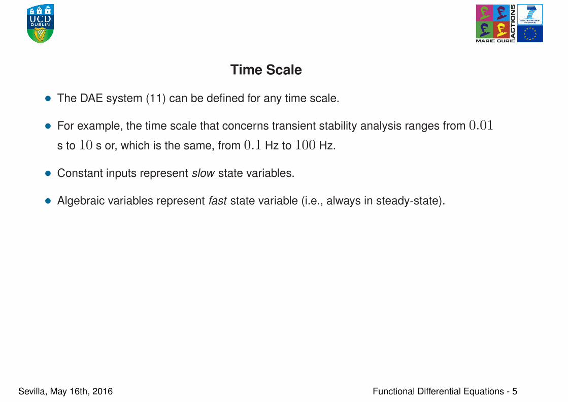
Limitations of First Lyapunov Method

• Equilibria characterized by ℜλi = 0 for some i, can be bifurcation points.

• In practice, there are only two relevant cases:

1. One eigenvalue is λk = 0. This condition often follows the occurrence of a

saddle-node bifurcation.

2. A pair of complex eigenvalues as zero real part, i.e., λh,k = ±jβ (e.g., Hopf

bifurcation).

• Bifurcation points are important because allow defining the stability margin of a current

operating point.


Small-signal stability of delayed DAE

Sevilla, May 16th, 2016 Small-signal stability of delayed DAE - 1

Introducing Delays

• Introducing time delays in (11) changes the DAE into a set of delay differential

algebraic equations (DDAE).

• For the sake of simplicity, we only consider ideal constant time delays:

yd = y(t− τ) (15)

where yd is the retarded or delayed variable with respect to some algebraic variable y,

t is the current simulation time, and τ (τ > 0) is the constant delay.

• A similar expression holds for delayed state variables:

xd = x(t− τ) (16)


Delay Differential Algebraic Equations

• Merging together DAE with (15) and (16) leads to:

x = f(x,y,xd,yd, t) (17)

0 = g(x,y,xd,yd, t)

• We consider first the case of a single scalar delay τ .

• Let’s restrict (for now) our analysis to index-1 Hessenberg form:

x = f(x,y,xd,yd, t) (18)

0 = g(x,y,xd, t)

Observe that g does not depend on yd.


Stationary Points of DDAEs (I)

• Assume that a stationary solution of (18) is known and has the form:

0 = f(x0,y0,x0,y0) (19)

0 = g(x0,y0,x0)

• Linearizing (18) at the stationary solution yields:

∆x = fx∆x+ f

xd∆xd + f

y∆y + f

yd∆yd (20)

0 = gx∆x+ g

xd∆xd + g

y∆y (21)


Stationary Points of DDAEs (II)

• Substituting (21) into (20), one obtains:

∆x = A0∆x+A1∆x(t− τ) +A2∆x(t− 2τ) (22)

where:

A0 = fx− f

yg−1y

gx

(23)

A1 = fxd

− fyg−1y

gxd

− fydg−1y

gx

(24)

A2 = −fydg−1y

gxd

(25)

• A0 is the well-known state matrix As that is computed for standard DAE systems.

• A2 = 0 if g do not depend on xd and/or f do not depend on yd.


Characteristic Equation (I)

• The substitution of a sample solution of the form eλtυ, with υ a non-trivial possibly

complex vector of order n, leads to the characteristic equation of (20)-(21):

det ∆(λ) = 0 (26)

where

∆(λ) = λIn −A0 −ν∑

i=1

Aie−λτi (27)

is called the characteristic matrix.

• For simplicity, assume only A1 6= 0, hence (27) becomes:

∆(λ) = λIn −A0 −A1e−λτ

(28)

• Note that the assumption is more restrictive than assuming the general index-1

Hessenberg form.


Roots of the Characteristic Equation

• The solutions of (27) are called the characteristic roots or spectrum, similar to the

finite-dimensional case (i.e., the case for which Ai = 0 ∀i = 1, . . . , ν ).

• However, since (27) is transcendental, it has infinitely many roots, and thus one can

only approximate the solution of (27) computing a reduced set of its roots.


Properties of the Characteristic Equation

• There are two useful properties of the characteristic matrix that allows its exploitation

for stability studies:

1. Equation (27) only has a finite number of characteristic roots in any vertical strip of

the complex plane, given by λ ∈ C : α < ℜ(λ) < β2. There exists a number γ ∈ R such that all characteristic roots of (27) are confined

to the half-plane λ ∈ C : ℜ(λ) < γ.

• These properties imply that the number of solutions in the right-half of the complex

plane is finite and, clearly, if γ ≤ 0, there is no eigenvalue with positive real part.

• Unfortunately, it is impossible to define a precise value for γ!


Solution of the Characteristic Equation

• Since the roots of the characteristic equation are infinite, only approximate solutions

are available.

• There are solutions based on frequency-domain methods that find an approximated

finite set of roots.

• Pade approximants: this approach consists in approximating the delay transfer function

as a rational polynomial.

• Time-domain methods are based on the Lyapunov-Krasovskii’s stability theorem and

the Razumikhin’s theorem (see for example LMI-based methods).


Pade Approximants (I)

• The Pade approximants consist in approximating the delay transfer function as a

rational polynomial (which is based on the Taylor expansion):

e−τs = 1− τs+(τs)2

2!− (τs)3

3!+ . . . (29)

≈ 1 + b1τs+ · · ·+ bm(τs)m

1 + a1τs+ · · ·+ an(τs)n(30)

where, generally n ≥ m.


Pade Approximants (II)

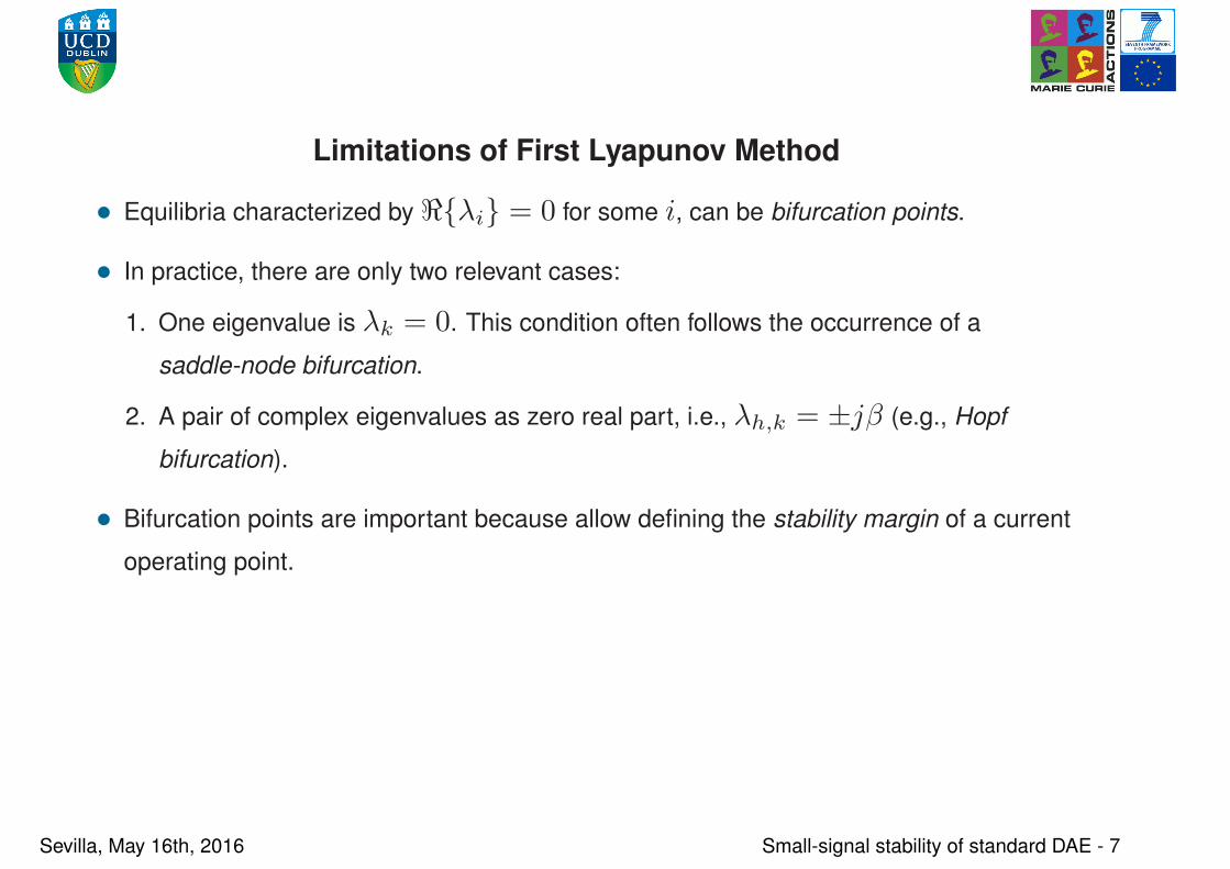
• Relevant cases are:

n = m = 0 ⇒ 1 (31)

n = 1, m = 0 ⇒ 1

1 + τs(32)

n = m = 1 ⇒ 1− τs/2

1 + τs/2(33)

n = 2, m = 1 ⇒ 1− τs/3

1 + 2τs/3 + (τs)2/6(34)

n = m = 2 ⇒ 1− τs/2 + (τs)2/12

1 + τs/2 + (τs)2/12(35)


Pade Approximants (III)

• If n = m, ai and bi coefficients are determined as follows:

a0 = 1 (36)

ai = ai−1n− i+ 1

i(2n− i+ 1)(37)

bi = ai(−1)i (38)

• A typical order used in computer applications is n = m = 6.


Frequency-domain Method (I)

• The idea is to transform the DDAE in a continuous boundary value problem with partial

derivatives (PDE) and then discretize using finite elements (Chebyshev’s discretization

scheme).

• Then, one has to choose the numbers of nodes composing Chebyshev’s discretization

scheme, say N .

• N affects the precision and the computational burden of the method.


Frequency-domain Method (II)

• The resulting matrix of which one has to compute the eigenvalues is of order N × n:

M =

C ⊗ In

A1 0 . . . 0 A0

(39)

where C is obtained eliminating the last n rows from C = −2DN/τ and DN is the

Chebyshev’s differentiation matrix of order N , and ⊗ is the Kronecker product.

• Then, the eigenvalues of M are an approximated spectrum of the original DDAE.


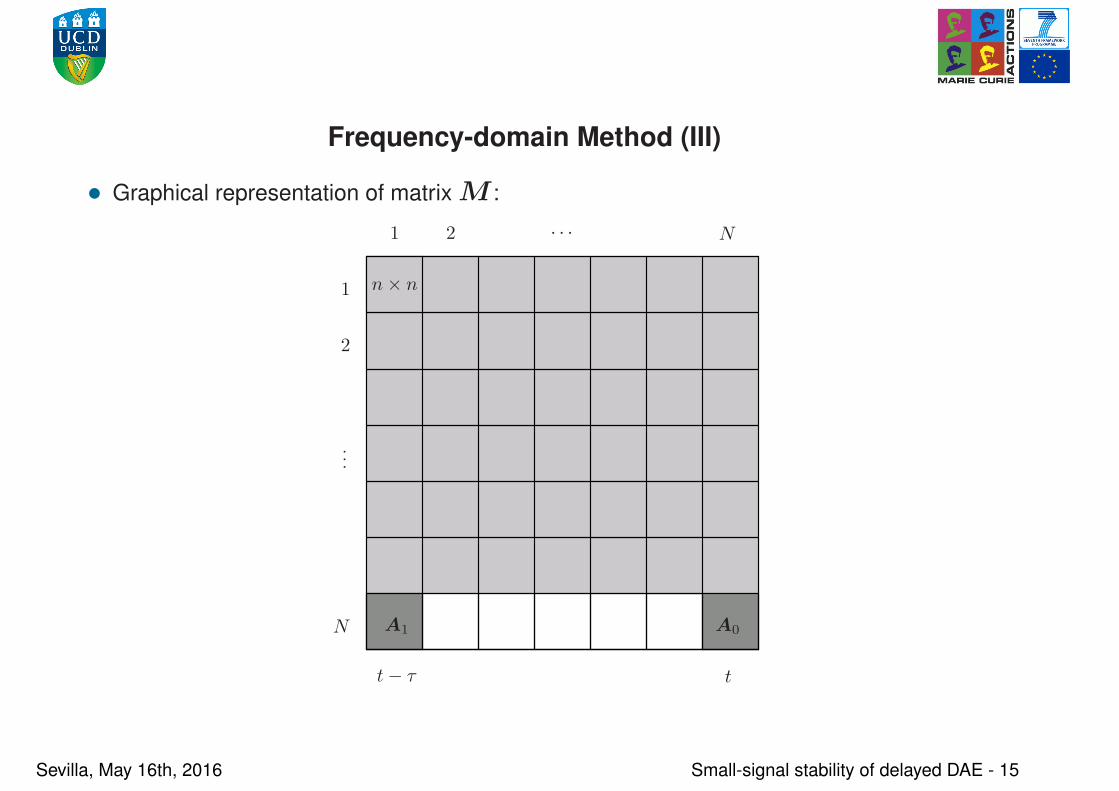
Frequency-domain Method (III)

• Graphical representation of matrix M :

t− τ t

1

1 2

2

N

N

.

.

.

. . .

A0A1

n× n


Removing the Hypothesis on A2

• We can easily take into account the general index-1 Hessenberg form.

• In this case, we have two delays: τ and 2τ .

• If we use odd N , matrix M becomes:

−2τ 0−τ

1

1 2

2

N

N

.

.

.

. . .

A0A1A2

n× n


Multiple Delay Case

• For the multiple delay case, we can adjust the matrices Aν using a linear interpolation

onto the Chebychev’s grid:

−τν 0−τν−1 −τν−2 −τ1−τ2

1

1

2

2

N

N

.

.

.

. . .


Removing the Hypothesis of Index-1 Hessenberg Form – I

• Index-1 Hessenberg form assumes that g do not depend on yd.

• If we remove this hypothesis, equation (22) becomes a summatory on infinite terms:

∆x = A0∆x+

∞∑

k=1

Ak∆x(t− kτ) (40)


Removing the Hypothesis of Index-1 Hessenberg Form – II

• Matrices in (40) are as follows:

A0 =fx+ f

yA , (41)

A1 =fxd

+ fydA+ f

yD , (42)

Ak =ECk−2D, k ≥ 2, (43)

where

A = −g−1y

gx, B = −g−1

ygxd

, (44)

C = −g−1y

gyd

, D = B +CA ,

E = fyC + f

yd.


Convergence of the Series

• The series in (40) converges if and only if ‖C‖ < 1, where ‖ · ‖ induced norm, or,

equivalently, if and only if ρ(C) < 1, where ρ(·) spectral radius of the eigenvalues of

a matrix.

• If ρ(C) < 1, the matrices Ak tend to 0p,p as k → ∞.

• Based on the definition of Ak in (43), the following condition must hold:

ρ(C) = ρ(g−1y

gyd) < 1 . (45)


Other Frequency-Domain Methods

• Discretization of the Time Integration Operator (TIO) as proposed by Bueler et al.

• Linear Multi-Step (LMS) approximation which has been proposed by Engelborghs et al.

and is implemented in the open-source software tool DDE-BIFTOOL

• These methods can account for the multiple-delay case.


Pros and Cons of Available Methods

• Pade approximants can easily take into account several different delays but introduces

phase inaccuracies for high frequencies.

• PDE discretization can have arbitrary precision (as N increases), but is numerically

demanding and gets complicated for the multiple delay case.

• Frequency-domain methods have a limited (or even null) ability to take into account

uncertainties or time dependency of the delays, whereas time-domain methods based

on Lyapunov-Krasovskii’s theorem can do that.

• Time-domain methods based on Lyapunov-Krasovskii’s theorem are limited to the

ability of defining a Lyapunov function, are inconclusive if the stability condition is not

satisfied, and do not allow to define a stability margin.


Numerical Libraries for Eigenvalue Analysis

Sevilla, May 16th, 2016 Numerical Libraries for Eigenvalue Analysis - 1

Algorithms to Compute Eigenvalues

• The problem can be tackled in two ways:

– To find the roots of a polynomial (slow even for small problems!)

– To find all eigenvalues and eigenvectors of the state matrix (e.g., Shur method and

QR decomposition). This is adequate for small to medium size problems.

– To find a subset of eigenvalues, based on some properties (e.g., largest magnitude,

smallest real part, etc.). This is probably the most promising approach for stability

analysis.


Some Libraries

• Full specturm:

– LAPACK: state-of-the-art of the QR factorization and Shur method.

– EISPACK: superseded by LAPACK.

– MAGMA: GPU-based Shur method.

– GSL: Double-shift Francis method

• Partial spectrum:

– ARPACK: it provides the state-of-the art for the Arnoldi iteration. It requires a good

algorithm to factorize the state matrix (e.g., KLU)

– SLEPc: it is based on PETSc and provides several algorithms: Arnoldi iteration,

Krylov-Shur method, Lanczos method, generalized Davidson method.

– HSL: Subspace iteration as well as Arnoldi itearation with Chebychev acceleration.


Z-domain - I

• While the S-domain is widely used in power system analysis, there are alternative

domain that can be used to solve the eigenvalue analysis.

• For example, Z-domain bilinear transformation is as follows:

AZ = (AS + χI)(AS − χInx)−1

(46)

where AS is the original state matrix, I the identity matrix of the same size as AS ,

and χ is a weighting factor that, based on heuristic considerations, can be set to

χ = 8.


Z-domain - II

• The first Lyapunov method applied to the Z-domain, becomes:

– If |λi| < 1 ∀ i = 1, . . . , n, the equilibrium point is asymptotically stable.

– If |λi| > 1 for some i, the equilibrium point is unstable.

– If |λi| = 1 for some i, further investigation is needed.


Z-domain - III

• Computing AZ is more expensive than AS but using AZ can be useful to:

– Better visualize stiff systems, as the eigenvalues falls within or close to the unitary

circle.

– To speed up the determination of the maximum amplitude eigenvalue (e.g., by

means of the Arnoldi iteration), especially in case of unstable equilibrium points with

only few eigenvalues outside the unit circle.


Test Case

• Comparison of different algorithms and libraries to compute the eigenvalues in the

Z-domain for the IEEE 14-bus system with time delays and N = 40.

• The total number of eigenvalues is 1960.

• Iterative methods compute the largest magnitude eigenvalues usin a tolerance of

10−4.

• All simulations are solved on a server equipped with two processors Intel Xeon Quad

Core 3.50 GHz, 12 GB of RAM, 1 GB NVidia Quadro 2000, and mounting a Linux 64

bits operating system.


Complexity of the Eigenvalue Problem

• The complexity of the eigenvalue problem scales to O(m3), where m is the

dimension of the matrix.

• These are some results using LAPACK and a variety of state matrix sizes.

# of Eigs. (m) Chebychev grid (N ) CPU time (s)

49 1 0.009

245 5 0.032

490 10 0.216

2450 50 38.07

4900 100 351.35


Performance of Different Libraries

Library Method # of Eigs. CPU time

LAPACK Shur method All 22.59 s

MAGMA GPU-based Shur method All 14.55 s

GSL Double-shift Francis method All 57.03 s

ARPACK Arnoldi Iter. & LAPACK 50 8.18 s

SLEPC Arnoldi Iter. & Krylov Subspace 79 7 m 38 s

SLEPC Krylov-Shur method 79 8 m 10 s

SLEPC Lanczos method 79 8 m 5 s

SLEPC Generalized Davidson method - not conv.

HSL Subspace Iter. with Chebychev acc. 50 3.56 s

HSL Arnoldi Iter. with Chebychev acc. 50 42.34 s


How do delays affect system stability?

Sevilla, May 16th, 2016 How do delays affect system stability? - 1

Example: IEEE 14-bus System with Delays (I)

• Let consider the IEEE 14-bus system.

• The system is composed of 5 generators with AVR.

• Let assume that the voltage measure of AVRs is affected by a delay τv :

vc = (vT (t− τv)− vc)/Tr (47)

where vc is the AVR measured voltage and vT the generator terminal voltage.

• The dynamic order of the considered system is nx = 49.


Example: IEEE 14-bus System with Delays (II)

THREE WINDING

C

C

G

G

C

9

TRANSFORMER EQUIVALENT

8

7

4

9

C

GENERATORS

2

1

5

78

4

1011

14

13

12

6

SYNCHRONOUS

COMPENSATORS

G

3

C


Example: IEEE 14-bus System with Delays (II)

• Computational burden of the spectrum analysis for τv = 5 ms and for the IEEE

14-bus system for different values of N .

N N · nx (N · nx)2 NNZ NNZ/(N · nx)

2

1 49 2 401 776 32.3%

5 245 59 049 1 707 2.83%

10 490 240 100 5 186 2.15%

20 980 960 400 19 396 2.02%

40 1 960 3 841 600 77 216 2.01%


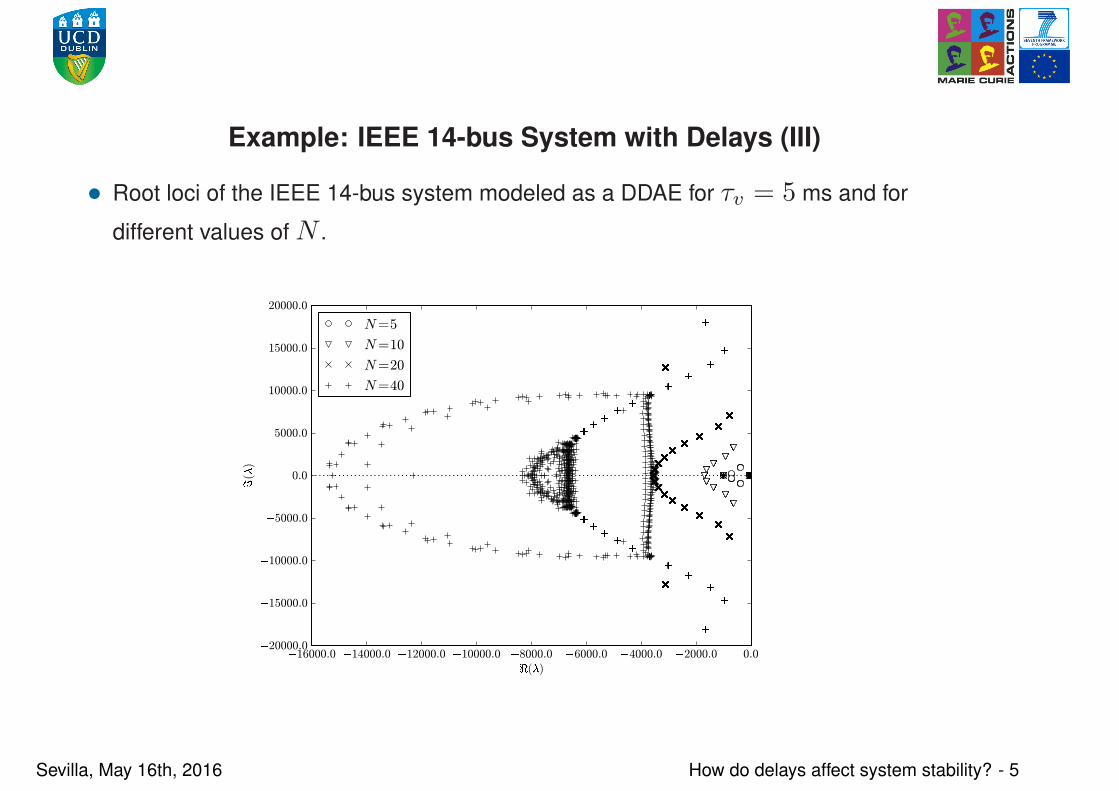
Example: IEEE 14-bus System with Delays (III)

• Root loci of the IEEE 14-bus system modeled as a DDAE for τv = 5 ms and for

different values of N .

16000.0 14000.0 12000.0 10000.0 8000.0 6000.0 4000.0 2000.0 0.0

( )

20000.0

15000.0

10000.0

5000.0

0.0

5000.0

10000.0

15000.0

20000.0

(

)

N=5

N=10

N=20

N=40


Example: IEEE 14-bus System with Delays (IV)

• Zoom close to the imaginary axis of the root loci of the IEEE 14-bus system modeled

as a DDAE for τv = 5 ms and for different values of N .

1.4 1.2 1.0 0.8 0.6 0.4 0.2 0.0

( )

10.0

5.0

0.0

5.0

10.0

(

)

N=5

N=10

N=20

N=40


Example: IEEE 14-bus System with Delays (V)

• Let now assume that the delay affects the measure of a PSS connected to generator 1.

• PSS may take a remote signal to damp oscillation, thus making possible relatively high

delays (e.g., > 100 ms).

• Generator 1 can be considered an equivalent of an external system with remote PSS

measure.


Example: IEEE 14-bus System with Delays (VI)

• Rotor speed ω of machine 5 for the IEEE 14-bus system with a 20% load increase

and for different control models following line 2-4 outage at t = 1 s.


Do Delays Always Destabilize the System?

• In spite of the “bad reputation” of delays as a source of destabilization, delays can also

have surprisingly positive effects on improving system stability.

• Let consider the case of a synchronous machine with a PSS.


Classical Machine Model (I)

• Consider the well-known simplified electromechanical model of a synchronous

machine in steady state:

2Hω

dt= pm − pe(δ), (48)

• ω is the rotor speed, H is the machine inertia constant, pm is the mechanical power,

and pe is the electromagnetical power defined as:

pe(δ) =e′qv

x′

d

sin(δ − θ), (49)

• δ is the rotor angle, v and θ are the machine bus terminal voltage magnitude and

phase angle, respectively, e′q is the internal fem, and x′

d is the d-axis transient

reactance.


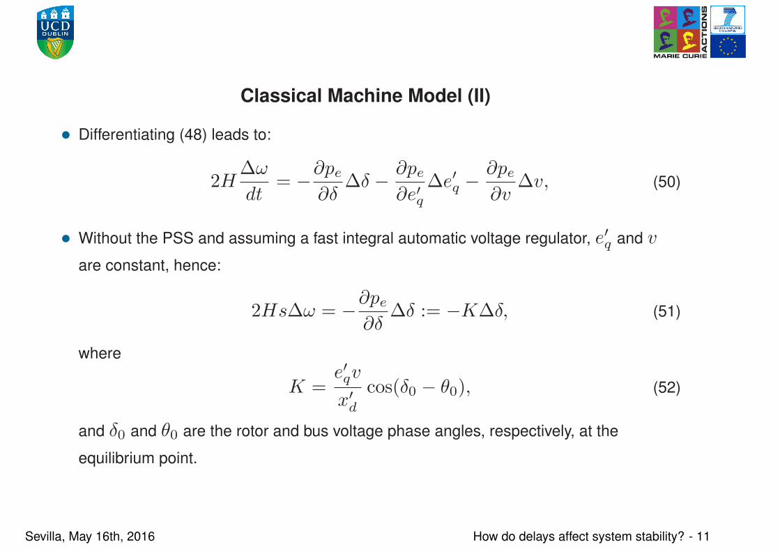
Classical Machine Model (II)

• Differentiating (48) leads to:

2H∆ω

dt= −∂pe

∂δ∆δ − ∂pe

∂e′q∆e′q −

∂pe∂v

∆v, (50)

• Without the PSS and assuming a fast integral automatic voltage regulator, e′q and v

are constant, hence:

2Hs∆ω = −∂pe∂δ

∆δ := −K∆δ, (51)

where

K =e′qv

x′

d

cos(δ0 − θ0), (52)

and δ0 and θ0 are the rotor and bus voltage phase angles, respectively, at the

equilibrium point.


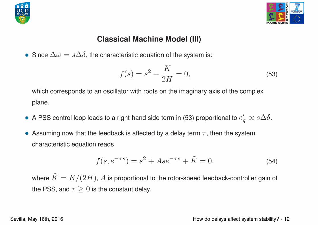
Classical Machine Model (III)

• Since ∆ω = s∆δ, the characteristic equation of the system is:

f(s) = s2 +K

2H= 0, (53)

which corresponds to an oscillator with roots on the imaginary axis of the complex

plane.

• A PSS control loop leads to a right-hand side term in (53) proportional to e′q ∝ s∆δ.

• Assuming now that the feedback is affected by a delay term τ , then the system

characteristic equation reads

f(s, e−τs) = s2 +Ase−τs + K = 0. (54)

where K = K/(2H), A is proportional to the rotor-speed feedback-controller gain of

the PSS, and τ ≥ 0 is the constant delay.


Classical Machine Model (IV)

• Stability map on A-τ plane for K ≈ 2.0. The power system is stable in the shaded

regions.

0.0 2.0 4.0 6.0 8.0 10.0

τ [s]

−2.0

−1.0

0.0

1.0

2.0

A∝

PSScontrollergain


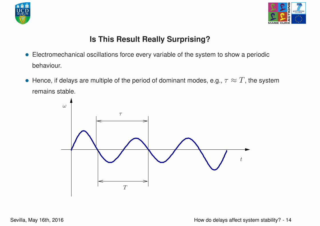
Is This Result Really Surprising?

• Electromechanical oscillations force every variable of the system to show a periodic

behaviour.

• Hence, if delays are multiple of the period of dominant modes, e.g., τ ≈ T , the system

remains stable.

ω

T

τ

t


IEEE 14-bus System (revisited)

• Stability map of the Kw-τω plane for the IEEE 14-bus system. Shaded regions are

stable. Dark shaded regions indicate a damping greater than 5%.

0.0 0.1 0.2 0.3 0.4 0.5Delay τω [s]

−5.0

0.0

5.0

10.0

15.0

20.0

PSScontrollergain

Kw


Large Power Systems – Multiple-Delay Case – I

• When it comes to compute the eigenvalues, the size does matter.

• We now consider a multi-delay case based on a dynamic model of the all-island Irish

transmission system.

• The model includes 1, 479 buses, 1, 851 transmission lines and transformers, 245

loads, 22 conventional synchronous power plants with AVRs and turbine governors, 6

PSSs and 176 wind power plants.

• For sake of example, constant time-delays are artificially included in most regulators of

the system.


All-Island Irish System

TRANSMISSION SYSTEM

400, 275, 220 AND 110kV

JANUARY 2014

HVDC


Large Power Systems – Multiple-Delay Case – II

• The system contains 296 delays ranging in the interval (0.005, 11) s.

Device Delayed Signal Delay Range [s]

Primary voltage regulator bus voltage τAVR

(0.005, 0.015)

Power system stabilizer frequency τPSS

(0.05, 0.25)

Reheater of steam turbines steam flow τTG

(3, 11)

Wind turbine freq. reg. frequency τTFR

(0.05, 0.25)

Therm. controlled load frequency τTCL

(0.05, 0.25)


Large Power Systems – Multiple-Delay Case – III

• Computational burden of different methods to compute eigenvalues

Model Settings Matrix setup Matrix order LEP sol.

No delays 1.18 s 2, 239 11.91 s

Cheb. discr. N = 7 29.4 s 13, 545 12.69 m

Discr. of TIO N · r = 21 7.07 h 40, 635 50.73 s

LMS approx. h = 0.2 s 7.48 m 32, 895 20.83 s

Pade approx. p = q = 6 2.01 s 3, 415 35.21 s

Pade approx. p = q = 10 2.78 s 4, 399 76.75 s


Large Power Systems – Multiple-Delay Case – IV

No delay Chebyshev Discr. Discr. of TIO LMS Approx. Pade Approx. Pade Approx.

N = 7 N · r = 21 h = 0.2 s p = q = 6 p = q = 10

−0.00010 −0.00010 −3.16992 0.91568 −0.00010 14370.508

−0.02500 −0.02500 −3.46994 0.82393 −0.02500 2166.5568

−0.02646 −0.02650 −3.54846 0.58361 −0.02848 1545.1549

−0.03780 ± 0.32935i −0.03780 ± 0.32935i −3.79015 0.36998 −0.03780 ± 0.32935i 1540.3456

−0.05475 −0.05475 −3.79481 0.29701 −0.05475 1445.2436

−0.06615 −0.06100 ± 0.32755i −3.85081 0.10980 −0.06615 1434.9052

−0.08759 ± 0.10409i −0.06615 −3.86392 −0.00327 −0.08759 ± 0.10409i 1019.4456

−0.11681 −0.08759 ± 0.10409i −4.25558 −0.05199 −0.10759 ± 0.33539i 891.50938

−0.12665 ± 0.34150i −0.11445 ± 0.78025i −4.33068 −0.09677 −0.11681 795.91920

−0.13055 ± 0.17132i −0.11681 −4.52052 −0.13551 −0.12906 ± 0.34552i 724.39851

−0.13922 −0.12818 ± 0.34639i −4.68635 −0.15511 −0.13380 ± 0.17103i 648.25856

−0.13950 −0.13455 ± 0.17176i −4.80909 −0.23989 −0.13417 625.18431

−0.13978 −0.17139 −4.84030 −0.32102 −0.17474 ± 0.27121i 593.37327

−0.14008 −0.17358 ± 0.27051i −5.24457 ± 0.35652i −0.34557 −0.17504 587.83144

−0.14027 −0.17504 −5.26514 −0.45854 −0.18411 ± 0.78161i 533.95381

−0.14048 −0.18208 ± 0.81259i −5.67946 ± 0.81568i −0.55539 −0.18562 528.11686

−0.14062 −0.18316 ± 0.81807i −5.74580 −0.67482 −0.18892 519.93536

−0.14081 −0.18562 −5.80760 −0.73128 −0.20000 497.91600


Long Transmission Lines – ∞-Delay Case – I

• Long transmission lines are best modelled through a continuum, which leads to the

well-known set of partial differential equations:

∂v(ℓ, t)

∂ℓ= Ri(ℓ, t) + L

∂i(ℓ, t)

∂t(55)

∂i(ℓ, t)

∂ℓ= Gv(ℓ, t) + C

∂v(ℓ, t)

∂t

where R, L, C and G are the resistance, inductance, capacitance and conductance

per unit length, respectively.

• Equations (55) along with the conditions:

v(0, t) = vi(t), v(ℓij , t) = vj(t) (56)

i(0, t) = ii(t), i(ℓij , t) = ij(t) = −ii(t)

where ℓij is the total length of the line, define a boundary value problem.


Long Transmission Lines – ∞-Delay Case – II

• Approximations are needed to solve (55).

• Assuming fast balanced time-varying phasors, the boundary value problem becomes:

∂v(ℓ, t)

∂ℓ= Ri(ℓ, t) + L

∂i(ℓ, t)

∂t+ jω0Li(ℓ, t) (57)

∂i(ℓ, t)

∂ℓ= Gv(ℓ, t) + C

∂v(ℓ, t)

∂t+ jω0Cv(ℓ, t)

v(0, t) = vi(t), v(ℓij , t) = vj(t)

i(0, t) = ii(t), i(ℓij , t) = ij(t)

where ω0 is the synchronous pulsation.


Long Transmission Lines – ∞-Delay Case – III

• Assuming G ≈ 0, the boundary value problem (57) has an explicit solution [?].

• Let define the following quantities:

– Characteristic admittance Yc =√

C/L.

– Time delay (or travelling time) τij = ℓij√LC , i.e., the time required by a wave to

pass through the line at the wave speed 1/√LC .

– Phase shift βij = ω0τij and attenuation factor αij =Rℓij2 Yc.


Long Transmission Lines – ∞-Delay Case – IV

• Then, (57) has the solution:

0 =− ii(t) + ii(t− 2τij)e−2(αij+jβij) − Ycwi(t) (58)

+ 2Ycwj(t− τij)e−(αij+jβij)

− Ycwi(t− 2τij)e−(αij+jβij)

0 =− ij(t) + ij(t− 2τij)e−2(αij+jβij) − Ycwj(t)

+ 2Ycwi(t− τij)e−(αij+jβij)

− Ycwj(t− 2τij)e−2(αij+jβij)


Long Transmission Lines – ∞-Delay Case – V

• wi and wj satisfy the following set of complex differential equations:

˙wi − ˙vi = −jω0wi −R

2Lwi + jω0vi (59)

˙wj − ˙vj = −jω0wj −R

2Lwj + jω0vj

• If R ≈ 0 (e.g., loss-less line), equations (58) become:

0 =− ii(t) + ii(t− 2τij)e−j2βij − Ycvi(t) (60)

+ 2Ycvj(t− τij)e−jβij − Ycvi(t− 2τij)e

−j2βij

0 =− ij(t) + ij(t− 2τij)e−j2βij − Ycvj(t)

+ 2Yij vi(t− τij)e−jβij − Ycvj(t− 2τij)e

−j2βij

• Equations (58)-(59) or (60) are a set of functional differential equations with constant

delays.


Long Transmission Lines – ∞-Delay Case – VI

• Equations (58)-(59) lead to:

x = f(x,y) (61)

0 = g(x,y,xd,yd).

where delayed quantities are transmission line transient voltages

xd = [wre,d,wim,d], with w = wre + jwim and currents yd = [ire,d, iim,d],

with i = ire + jiim.

• Equations (60) lead to:

x = f(x,y) (62)

0 = g(x,y,yd).

where delayed quantities are only transmission line currents yd = [ire,d, iim,d].


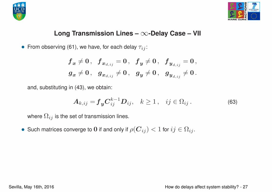
Long Transmission Lines – ∞-Delay Case – VII

• From observing (61), we have, for each delay τij :

fx6= 0 , f

xd,ij= 0 , f

y6= 0 , f

yd,ij= 0 ,

gx6= 0 , g

xd,ij6= 0 , g

y6= 0 , g

yd,ij6= 0 .

and, substituting in (43), we obtain:

Ak,ij =fyCk−1

ij Dij , k ≥ 1 , ij ∈ Ωij . (63)

where Ωij is the set of transmission lines.

• Such matrices converge to 0 if and only if ρ(Cij) < 1 for ij ∈ Ωij .


Long Transmission Lines – ∞-Delay Case – VIII

• Loss-less line model (62) shows same Jacobian matrices as (61) but for

gxd,ij

= 0q,p, which leads to:

Ak,ij =fyCk

ijAij , k ≥ 1 , ij ∈ Ωij . (64)


Long Transmission Lines – ∞-Delay Case – IX

• It is possible to show that the spectral radius of transmission lines modelled with

(58)-(59) satisfy the condition

ρ(Cij) = e−2αij . (65)

• The spectral radius of transmission lines modelled with (60) satisfies the condition

ρ(Cij) = 1.

• The latter can be easily shown by observing that loss-less transmission lines have

R = 0, and, hence, by the definition of the attenuation factor, αij = 0.


IEEE 39-bus system – I

• The IEEE 39-bus system is utilized to illustrate the effect of transmission line delays.

• Let’s assume that four lines are long.

• Lengths, attenuation factors and delays of four transmission lines of the New England

39-bus system.

Line i-j ℓij [km] αij [Np] e−αij e−2αij τij [ms]

1-2 276 0.0179 0.9822 0.9648 1.131

23-24 234 0.0152 0.9849 0.9700 0.962

25-26 216 0.0141 0.9860 0.9723 0.887

26-29 418 0.0271 0.9732 0.9472 1.713


IEEE 39-bus system – II

• We consider three cases:

• Standard lumped models of transmission lines

• Dynamic delay models of the lines with attenuation, i.e., models (58)-(59), which

lead to the DDAE as in (61);

• Delay loss-less line models (60), which lead to the DDAE as in (62).

• For the DDAEs, we have truncated the series at the first 50 terms and used a

Chebyshev grid with N = 10 nodes.


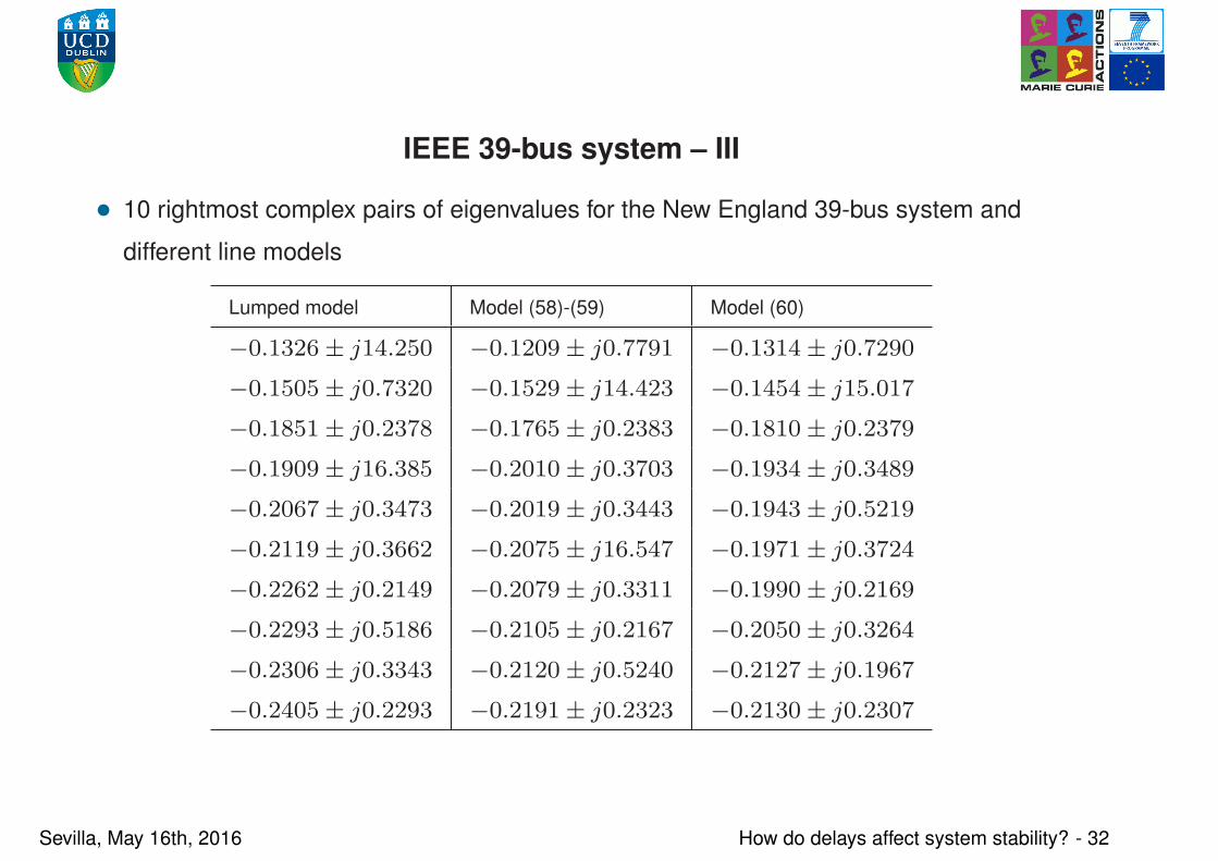
IEEE 39-bus system – III

• 10 rightmost complex pairs of eigenvalues for the New England 39-bus system and

different line models

Lumped model Model (58)-(59) Model (60)

−0.1326± j14.250 −0.1209± j0.7791 −0.1314± j0.7290

−0.1505± j0.7320 −0.1529± j14.423 −0.1454± j15.017

−0.1851± j0.2378 −0.1765± j0.2383 −0.1810± j0.2379

−0.1909± j16.385 −0.2010± j0.3703 −0.1934± j0.3489

−0.2067± j0.3473 −0.2019± j0.3443 −0.1943± j0.5219

−0.2119± j0.3662 −0.2075± j16.547 −0.1971± j0.3724

−0.2262± j0.2149 −0.2079± j0.3311 −0.1990± j0.2169

−0.2293± j0.5186 −0.2105± j0.2167 −0.2050± j0.3264

−0.2306± j0.3343 −0.2120± j0.5240 −0.2127± j0.1967

−0.2405± j0.2293 −0.2191± j0.2323 −0.2130± j0.2307


Thanks for your attention!

Sevilla, May 16th, 2016 Thanks! - 1

Modelling and Stability Analysis of Power Systems with...

Documents

Transcript of Modelling and Stability Analysis of Power Systems with...