Modelling and Simulation of the Coupled Rigid-flexible ... · PDF fileModelling and Simulation...

Modelling and Simulation of the Coupled Rigid-flexible Multibody

Systems in MWorks

Xie Gang1, Zhao Yan

1, Zhou Fanli*

2, Chen Liping

1

1CAD Center, Huazhong University of Science and Technology, Wuhan, China, 430074

2Suzhou Tongyuan Software & Control Tech. Co. Ltd, Suzhou, China, 215123

{xieg, zhaoy, zhoufl, chenlp}@tongyuan.cc

Abstract

Aiming to the design challenge of modern mecha-

tronic products, this paper presents a method to sim-

ulate the coupled rigid-flexible system in MWorks.

Firstly, the component mode synthesis (CMS) tech-

nique is introduced and the Craig-Bampton method

is adopted to build the flexible-body model. The

general flexible-body model named FlexibleBody is

developed based on the standard MultiBody library

in Modelica, which describes the small and linear

deformation behavior (relative to a local reference

frame) of a flexible-body that undergoes large and

non-linear global motion. In the model, the modal

neutral file (MNF) is introduced as a standard inter-

face to describe the constraint modes. Secondly, the

model is used to construct a library of boom system

of concrete pump truck and the simulations covering

the expanding and folding process are carried out

based on both the rigid multibody and the coupled

rigid-flexible system models. Finally, the influence

to dynamics performance of the boom system is ana-

lyzed and the conclusion is drawn. The method in

this paper provides an effective approach to build

unified model and simulate flexible-body in multi-

domain engineering systems.

Keywords: rigid-flexible system; concrete pump

truck; MWorks

1 Introduction

Much industrial equipment is mechatronic and con-

tains high-speed, lightweight, and high-precision

mechanical system. In these mechanical systems one

or more structural components often need to consider

the deformation effects for design analyses. The in-

tegrated design and simulation of the mechatronic

systems with flexible bodies make the multidiscipli-

nary challenge. When designing such a mechatronic

system, the performance requirements must be satis-

fied and the strength of the system must be guaran-

teed. Therefore, stress and deformation of machine

components have to be predicted in the design pro-

cess.

The increasing computational power of current com-

puter enables to model a multibody system as 3D

deformable body using the finite element method.

The flexible multibody dynamics is the subject con-

cerned with the modeling and analysis of constrained

deformable bodies that undergo large displacements

and rotations. DLR® FlexibleBodies Library [1, 2]

pro-

vides the general flexible model so that users can

simulate the elastic deformation of flexible-body in a

modal synthesis way, in which the standard input

data (SID) [3, 4]

file should be offered by a third-party

software. In SID file, Guyan reduction and Ritz ap-

proximation are adopted. The Rayleigh–Ritz method

[4] chooses an approximate form for the eigenfunc-

tion with the lowest eigenvalue. In the Guyan reduc-

tion method [4]

, a set of user-defined master nodes are

retained and the remaining set of slave nodes are re-

moved by condensation. Only stiffness properties are

considered during the condensation, and inertia cou-

pling of master and slave nodes are ignored. Based

on an improved Craig-Bampton method [5-8]

,

MSC.ADAMS® adopts the modal neutral file [9]

,

which can be exported by some finite element soft-

ware, to drive the animation of the flexible body.

The MNF is a binary file that contains the location of

nodes and node connectivity, nodal mass and inertia,

mode shapes, generalized mass and stiffness for

mode shapes. The mode shapes in modal neutral file,

which contain the interface constraint modes, are

revised effectively after modal truncation. So the

Craig-Bampton method is more accurate and has

been widely used in engineering [10-14]

. But the soft-

ware, just like ADAMS, mainly focuses on modeling

and simulation of the pure mechanical system and

lacks support of multi-domain physical systems. In

order to model and simulate the mechatronic prod-

ucts composed of mechanical, electronic, hydraulic,

and control engineering systems, the co-simulation

DOI Proceedings of the 9th International Modelica Conference 405 10.3384/ecp12076405 September 3-5, 2012, Munich, Germany

should be performed with other software such as

Matlab/Simulink®, LMS.AMESim®, etc.

In this paper, the FlexibleBody model is developed

based on the component mode synthesis (CMS) and

the improved Craig-Bampton method [9, 11]

. An exter-

nal C function MNFParser is programmed to get the

mode shapes data in the model. The finite element

analysis (FEA) results can then be incorporated into

a part model by superimposing the flexible-body de-

flection on the motion of rigid-body. The postproces-

sor tool in MWorks [15]

is also improved to support

the nephogram animation of the deformation. As an

example, a boom system library of the concrete

pump truck is developed. And the simulations cover-

ing the expanding and folding process are carried out

based on both the rigid multibody and the coupled

rigid-flexible system models. The simulation results

are compared and it shows the coupled rigid-flexible

system is more conformable with the actual boom

system.

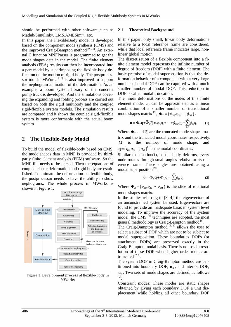
2 The Flexible-Body Model

To build the model of flexible-body based on CMS,

the mode shapes data in MNF is provided by third-

party finite element analysis (FEM) software. So the

MNF file needs to be parsed. Then the equations of

coupled elastic deformation and rigid body are estab-

lished. To animate the deformation of flexible-body,

the postprocessor needs to have the ability to show

nephograms. The whole process in MWorks is

shown in Figure 1.

Multi-domain Modeling

Computation

PostProcessor

Mw

orks

FlexibleBody

MnfParser

deformation nephograms

Parse MNF file

Calculate Invariants and Damping

Coefficient

Parameters

Variables

Initial Equations

EquationsMass, Inertia tenser, Node coordinate, etc.

MNF file name

Import geometry file

Render nephograms

Color legend bar

CAE software: Ansys, Nastran, etc.

MNF file

Initial algorithm

Figure 1: Development process of flexible-body in

MWorks

2.1 Theoretical Background

In this paper, only small, linear body deformations

relative to a local reference frame are considered,

while that local reference frame indicates large, non-

linear global motion.

The discretization of a flexible component into a fi-

nite element model represents the infinite number of

degree of freedom (DOF) with a finite element. The

basic premise of modal superposition is that the de-

formation behavior of a component with a very large

number of nodal DOF can be captured with a much

smaller number of modal DOF. This reduction in

DOF is called modal truncation.

The linear deformations of the nodes of this finite

element mode, u , can be approximated as a linear

combination of a smaller number of translational

mode shapes matrix [9]

, 1 2, , ,T T T TM Φ .

1 1

1

+ + + =M

T T T TM M Ti i

i

q q q

u Φ q Φ q (1)

Where TΦ and q are the truncated mode shapes ma-

trix and the truncated modal coordinates respectively.

M is the number of mode shape, and

1 2, , ,T

Mq q qq is the modal coordinates.

Similar to equation(1), as the body deforms, every

node rotates through small angles relative to its ref-

erence frame. These angles are obtained using a

modal superposition [9]

.

1

M

R R Ri i

i

q

θ Φ q Φ q (2)

Where 1 2, ,R R R RM Φ is the slice of rotational

mode shapes matrix.

In the studies referring to [3, 4], the eigenvectors of

an unconstrained system be used. Eigenvectors are

found to provide an inadequate basis in system level

modeling. To improve the accuracy of the system

model, the CMS [3]

techniques are adopted, the most

general methodology is Craig-Bampton method [5]

.

The Craig-Bampton method [5, 6]

allows the user to

select a subset of DOF which are not to be subject to

modal superposition. These boundaries DOFs (or

attachment DOFs) are preserved exactly in the

Craig-Bampton modal basis. There is no loss in reso-

lution of these DOF when higher order modes are

truncated [7, 8]

.

The system DOF in Craig-Bampton method are par-

titioned into boundary DOF, Bu , and interior DOF,

Iu . Two sets of mode shapes are defined, as follows [9]

:

Constraint modes: These modes are static shapes

obtained by giving each boundary DOF a unit dis-

placement while holding all other boundary DOF

Modelling and Simulation of the Coupled Rigid-flexible Multibody Systems in MWorks

406 Proceedings of the 9th International Modelica Conference DOI September 3-5, 2012, Munich Germany 10.3384/ecp12076405

fixed. The basis of constraint modes completely

spans all possible motions of the boundary DOFs,

with a one-to-one correspondence between the modal

coordinates of the constraint modes and the dis-

placement in the corresponding boundary DOF,

C Bq u .

Fixed-boundary normal modes: These modes are

obtained by fixing the boundary DOF and computing

an eigensolution. There are as many fixed-boundary

normal modes as the user desires. These modes de-

fine the modal expansion of the interior DOF. The

quality of this modal expansion is proportional to the

number of modes retained by the user.

The relationship between the physical DOF and the

Craig-Bampton modes and their modal coordinates is

illustrated by the following equation.

CB

IC IN NI

I 0 quu

Φ Φ qu (3)

Where I , 0 are identity and zeros matrices, respec-

tively. ICΦ is the physical displacements of the inte-

rior DOF in the constraint modes. INΦ is the physi-

cal displacements of the interior DOF in the normal

modes. Cq is the modal coordinates of the constraint

modes. Nq is the modal coordinates of the fixed-

boundary normal modes.

The generalized stiffness and mass matrices corre-

sponding to the Craig-Bampton modal basis are ob-

tained via a modal transformation.

2.2 FlexibleBody Model

The governing differential equation of flexible-body

[9, 15], in terms of the generalized coordinates is:

1

2

T T

g

M ψMξ Mξ ξ ξ Kξ f Dξ λ Q

ξ ξ (4)

Where,

,ξ,ξ ξ are the generalized coordinates of the flexible-

body and their time derivatives.

, 1, ,

T T

i i Mx y z q

ξ x ψ q

M is the mass matrix.

K is the generalized stiffness matrix.

gf is the generalized gravitational force.

D is the modal damping matrix.

Ψ is the algebraic constraint equations.

λ is the Lagrange multipliers for the constraints.

Q is the generalized applied forces.

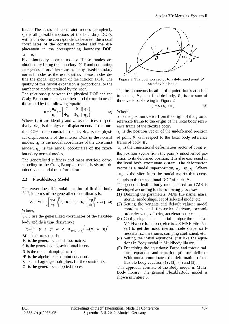
Figure 2: The position vector to a deformed point P

on a flexible body

The instantaneous location of a point that is attached

to a node, P , on a flexible body, B , is the sum of

three vectors, showing in Figure 2.

p p p r x s u (5)

Where

x is the position vector from the origin of the ground

reference frame to the origin of the local body refer-

ence frame of the flexible body.

ps is the position vector of the undeformed position

of point P with respect to the local body reference

frame of body B .

pu is the translational deformation vector of point P ,

the position vector from the point’s undeformed po-

sition to its deformed position. It is also expressed in

the local body coordinate system. The deformation

vector is a modal superposition, P TPu Φ q . Where

TPΦ is the slice from the modal matrix that corre-

sponds to the translational DOF of node P .

The general flexible-body model based on CMS is

developed according to the following processes.

(1) Defining the parameters: MNF file name, mass,

inertia, mode shape, set of selected mode, etc.

(2) Setting the variants and default values: modal

coordinates and first-order derivate, second-

order derivate, velocity, acceleration, etc.

(3) Configuring the initial algorithm: Call

MNFParser function (refer to 2.3 MNF File Par-

ser) to get the mass, inertia, mode shape, stiff-

ness matrix, invariants, damping coefficient, etc.

(4) Setting the initial equations: just like the equa-

tions in Body model in Multibody library.

(5) Describing the equations: Force and torque bal-

ance equation, and equation (4) are defined.

With modal coordinates, the deformation of the

flexible-body equation (1) , (2), (4) and (5).

This approach consists of the Body model in Multi-

Body library. The general FlexibleBody model is

shown in Figure 3.

Session 3D: Mechanic Systems II


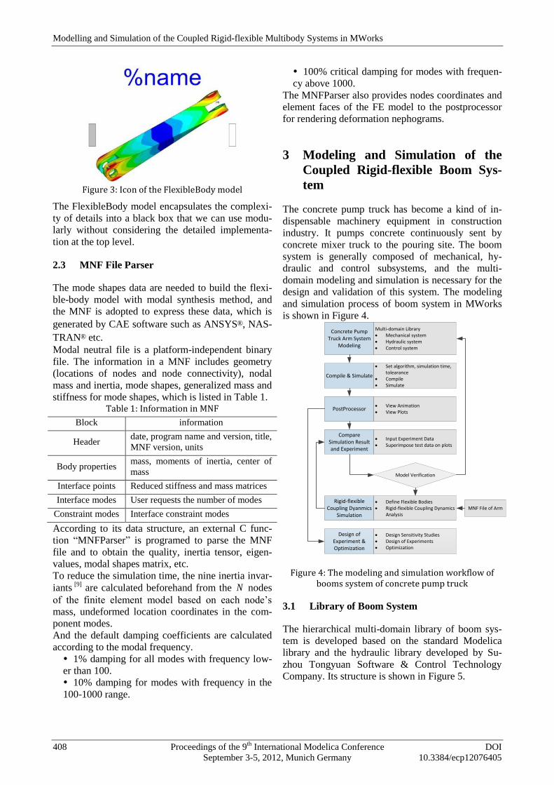
Figure 3: Icon of the FlexibleBody model

The FlexibleBody model encapsulates the complexi-

ty of details into a black box that we can use modu-

larly without considering the detailed implementa-

tion at the top level.

2.3 MNF File Parser

The mode shapes data are needed to build the flexi-

ble-body model with modal synthesis method, and

the MNF is adopted to express these data, which is

generated by CAE software such as ANSYS®, NAS-

TRAN® etc.

Modal neutral file is a platform-independent binary

file. The information in a MNF includes geometry

(locations of nodes and node connectivity), nodal

mass and inertia, mode shapes, generalized mass and

stiffness for mode shapes, which is listed in Table 1. Table 1: Information in MNF

Block information

Header date, program name and version, title,

MNF version, units

Body properties mass, moments of inertia, center of

mass

Interface points Reduced stiffness and mass matrices

Interface modes User requests the number of modes

Constraint modes Interface constraint modes

According to its data structure, an external C func-

tion “MNFParser” is programed to parse the MNF

file and to obtain the quality, inertia tensor, eigen-

values, modal shapes matrix, etc.

To reduce the simulation time, the nine inertia invar-

iants [9]

are calculated beforehand from the N nodes

of the finite element model based on each node’s

mass, undeformed location coordinates in the com-

ponent modes.

And the default damping coefficients are calculated

according to the modal frequency.

1% damping for all modes with frequency low-

er than 100.

10% damping for modes with frequency in the

100-1000 range.

100% critical damping for modes with frequen-

cy above 1000.

The MNFParser also provides nodes coordinates and

element faces of the FE model to the postprocessor

for rendering deformation nephograms.

3 Modeling and Simulation of the

Coupled Rigid-flexible Boom Sys-

tem

The concrete pump truck has become a kind of in-

dispensable machinery equipment in construction

industry. It pumps concrete continuously sent by

concrete mixer truck to the pouring site. The boom

system is generally composed of mechanical, hy-

draulic and control subsystems, and the multi-

domain modeling and simulation is necessary for the

design and validation of this system. The modeling

and simulation process of boom system in MWorks

is shown in Figure 4.

Concrete Pump Truck Arm System

Modeling

Multi-domain Library· Mechanical system· Hydraulic system· Control system

Compile & Simulate

· Set algorithm, simulation time, tolearance

· Compile· Simulate

PostProcessor· View Animation· View Plots

Compare Simulation Result and Experiment

· Input Experiment Data· Superimpose test data on plots

Model Verification

Rigid-flexible Coupling Dyanmics

Simulation

· Define Flexible Bodies· Rigid-flexible Coupling Dynamics

Analysis

Design of Experiment & Optimization

· Design Sensitivity Studies· Design of Experiments· Optimization

MNF File of Arm

Figure 4: The modeling and simulation workflow of

booms system of concrete pump truck

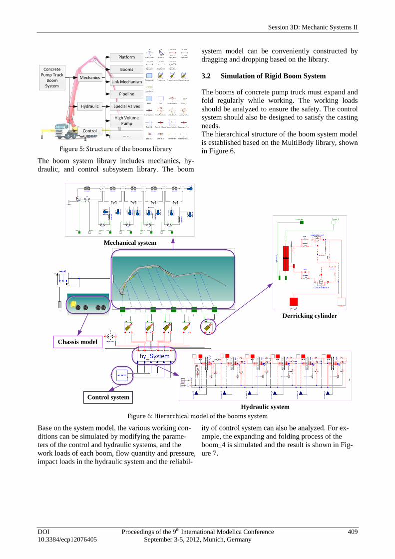
3.1 Library of Boom System

The hierarchical multi-domain library of boom sys-

tem is developed based on the standard Modelica

library and the hydraulic library developed by Su-

zhou Tongyuan Software & Control Technology

Company. Its structure is shown in Figure 5.



Concrete Pump Truck

Boom System

Mechanics

Hydraulic

Control

Platform

Booms

Link Mechanism

Pipeline

Special Valves

High Volume Pump

… ...

Figure 5: Structure of the booms library

The boom system library includes mechanics, hy-

draulic, and control subsystem library. The boom

system model can be conveniently constructed by

dragging and dropping based on the library.

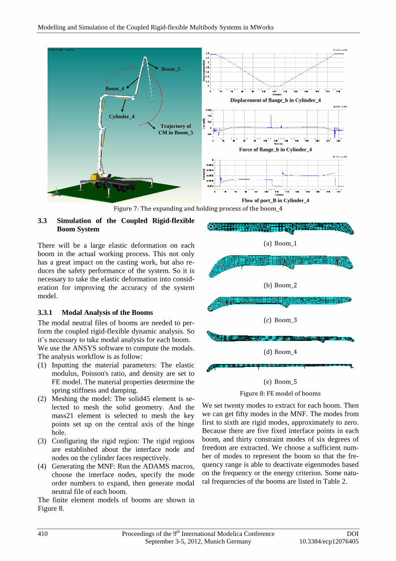
3.2 Simulation of Rigid Boom System

The booms of concrete pump truck must expand and

fold regularly while working. The working loads

should be analyzed to ensure the safety. The control

system should also be designed to satisfy the casting

needs.

The hierarchical structure of the boom system model

is established based on the MultiBody library, shown

in Figure 6.

Mechanical system

Derricking cylinder

Hydraulic system

Control system

Chassis model

Figure 6: Hierarchical model of the booms system

Base on the system model, the various working con-

ditions can be simulated by modifying the parame-

ters of the control and hydraulic systems, and the

work loads of each boom, flow quantity and pressure,

impact loads in the hydraulic system and the reliabil-

ity of control system can also be analyzed. For ex-

ample, the expanding and folding process of the

boom_4 is simulated and the result is shown in Fig-

ure 7.



Boom_4Boom_4

Boom_5Boom_5

Trajectory of

CM in Boom_5

Trajectory of

CM in Boom_5

Cylinder_4Cylinder_4

Displacement of flange_b in Cylinder_4

Force of flange_b in Cylinder_4

Flow of port_B in Cylinder_4 Figure 7: The expanding and holding process of the boom_4

3.3 Simulation of the Coupled Rigid-flexible

Boom System

There will be a large elastic deformation on each

boom in the actual working process. This not only

has a great impact on the casting work, but also re-

duces the safety performance of the system. So it is

necessary to take the elastic deformation into consid-

eration for improving the accuracy of the system

model.

3.3.1 Modal Analysis of the Booms

The modal neutral files of booms are needed to per-

form the coupled rigid-flexible dynamic analysis. So

it’s necessary to take modal analysis for each boom.

We use the ANSYS software to compute the modals.

The analysis workflow is as follow:

(1) Inputting the material parameters: The elastic

modulus, Poisson's ratio, and density are set to

FE model. The material properties determine the

spring stiffness and damping.

(2) Meshing the model: The solid45 element is se-

lected to mesh the solid geometry. And the

mass21 element is selected to mesh the key

points set up on the central axis of the hinge

hole.

(3) Configuring the rigid region: The rigid regions

are established about the interface node and

nodes on the cylinder faces respectively.

(4) Generating the MNF: Run the ADAMS macros,

choose the interface nodes, specify the mode

order numbers to expand, then generate modal

neutral file of each boom.

The finite element models of booms are shown in

Figure 8.

(a) Boom_1

(b) Boom_2

(c) Boom_3

(d) Boom_4

(e) Boom_5

Figure 8: FE model of booms

We set twenty modes to extract for each boom. Then

we can get fifty modes in the MNF. The modes from

first to sixth are rigid modes, approximately to zero.

Because there are five fixed interface points in each

boom, and thirty constraint modes of six degrees of

freedom are extracted. We choose a sufficient num-

ber of modes to represent the boom so that the fre-

quency range is able to deactivate eigenmodes based

on the frequency or the energy criterion. Some natu-

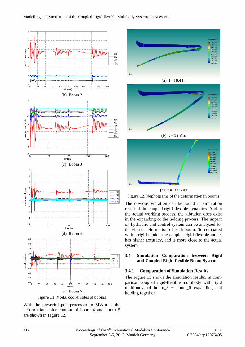
ral frequencies of the booms are listed in Table 2.



Table 2: Natural frequency of booms

Nat.

Freq. Boom_1 Boom_2 Boom_3 Boom_4 Boom4

1-6 0 0 0 0 0

7 25.8302 35.5842 33.0956 49.3527 8.7492

8 36.3539 48.4689 49.3527 22.1214 11.1239

9 52.8219 76.9397 49.3527 53.6334 23.7672

10 74.1143 89.2075 49.3527 60.5197 30.3335

11 75.6471 90.2372 49.3527 81.8889 47.3777

12 81.2592 94.7992 49.3527 85.3635 56.8012

… … … … … …

3.3.2 Replacement of the FlexibleBody Model

The rigid parts of booms shown in Figure 6 are re-

placed by FlexibleBody model with respective pa-

rameters, as shown in Figure 9. So the model of the

mechanical system is converted from the rigid multi-

body to the coupled rigid-flexible system.

Replaced by FlexibleBody model with respective parameters

Figure 9: The coupled rigid-flexible mechanical system

3.3.3 Simulation of Coupled Rigid-flexible

Boom System

The expanding and folding process of boom_5 is

simulated, as shown in Figure 10.

Flexible

Boom_4

Flexible

Boom_4

Flexible

Boom_5

Flexible

Boom_5

Trajectory of

CM in Boom_5

Trajectory of

CM in Boom_5

Cylinder_5Cylinder_5

Displacement of flange_b in Cylinder_5

Force of flange_b in Cylinder_5

Deformation of Boom_5

Figure 10: The process of expanding and folding boom_5

The modal coordinates of each boom are show in

Figure 11. The modal coordinates q[1] - q[6] are cor-

responding to 7th - 12

th modes respectively. Obvious-

ly, the value of modal coordinate q[1] is the biggest

one in each boom. It indicates that the 7th mode con-

tributes most energy to the flexible-body. And the

values of other modal coordinates are smaller and

smaller, indicating less energy contribution. The var-

iation tendency is complied with the modal superpo-

sition theorem and energy criterion

[11].

(a) Boom 1



(b) Boom 2

(c) Boom 3

(d) Boom 4

(e) Boom 5

Figure 11: Modal coordinates of booms

With the powerful post-processor in MWorks, the

deformation color contour of boom_4 and boom_5

are shown in Figure 12.

(a) t= 10.44s

(b) t = 12.84s

(c) t = 100.20s

Figure 12: Nephograms of the deformation in booms

The obvious vibration can be found in simulation

result of the coupled rigid-flexible dynamics. And in

the actual working process, the vibration does exist

in the expanding or the holding process. The impact

on hydraulic and control system can be analyzed for

the elastic deformation of each boom. So compared

with a rigid model, the coupled rigid-flexible model

has higher accuracy, and is more close to the actual

system.

3.4 Simulation Comparation between Rigid

and Coupled Rigid-flexible Boom System

3.4.1 Comparation of Simulation Results

The Figure 13 shows the simulation results, in com-

parison coupled rigid-flexible multibody with rigid

multibody, of boom_3 ~ boom_5 expanding and

holding together.



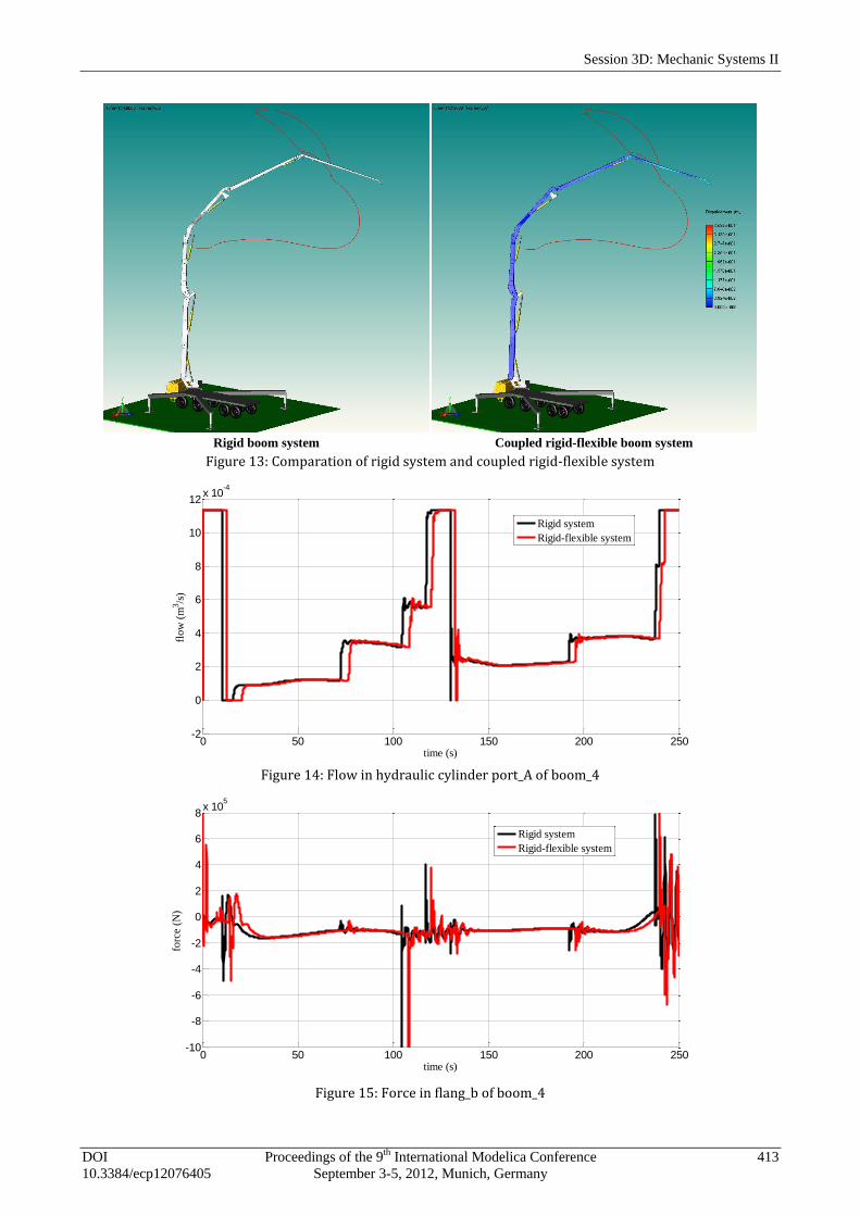
Rigid boom system Coupled rigid-flexible boom system Figure 13: Comparation of rigid system and coupled rigid-flexible system

Figure 14: Flow in hydraulic cylinder port_A of boom_4

Figure 15: Force in flang_b of boom_4

0 50 100 150 200 250-2

0

2

4

6

8

10

12x 10

-4

time (s)

flow

(m

3/s

)

Rigid system

Rigid-flexible system

0 50 100 150 200 250-10

-8

-6

-4

-2

0

2

4

6

8x 10

5

time (s)

forc

e (

N)

Rigid system




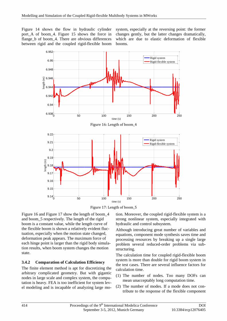
Figure 14 shows the flow in hydraulic cylinder

port_A of boom_4. Figure 15 shows the force in

flange_b of boom_4. There are obvious differences

between rigid and the coupled rigid-flexible boom

system, especially at the reversing point: the former

changes gently, but the latter changes dramatically,

which are due to elastic deformation of flexible

booms.

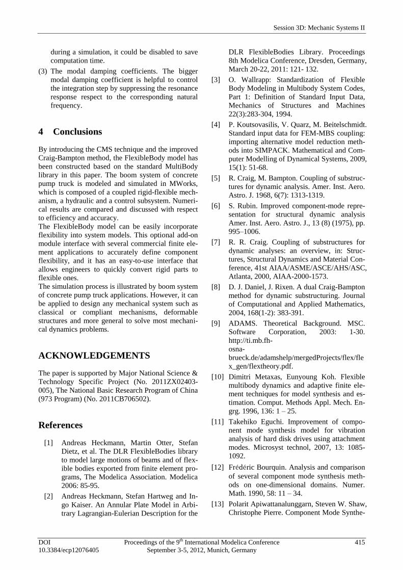
Figure 16: Length of boom_4

Figure 17: Length of boom_5

Figure 16 and Figure 17 show the length of boom_4

and boom_5 respectively. The length of the rigid

boom is a constant value, while the length curve of

the flexible boom is shown a relatively evident fluc-

tuation, especially when the motion state changed,

deformation peak appears. The maximum force of

each hinge point is larger than the rigid body simula-

tion results, when boom system changes the motion

state.

3.4.2 Comparation of Calculation Efficiency

The finite element method is apt for discretizing the

arbitrary complicated geometry. But with gigantic

nodes in large scale and complex system, the compu-

tation is heavy. FEA is too inefficient for system lev-

el modeling and is incapable of analyzing large mo-

tion. Moreover, the coupled rigid-flexible system is a

strong nonlinear system, especially integrated with

hydraulic and control subsystem.

Although introducing great number of variables and

equations, component mode synthesis saves time and

processing resources by breaking up a single large

problem several reduced-order problems via sub-

structuring.

The calculation time for coupled rigid-flexible boom

system is more than double for rigid boom system in

the test cases. There are several influence factors for

calculation time.

(1) The number of nodes. Too many DOFs can

mean unacceptably long computation time.

(2) The number of modes. If a mode does not con-

tribute to the response of the flexible component

0 50 100 150 200 2506.938

6.94

6.942

6.944

6.946

6.948

6.95

6.952

time (s)

length

(m

)

Rigid system


0 50 100 150 200 2509.14

9.15

9.16

9.17

9.18

9.19

9.2

9.21

9.22

time (s)

length

(m

)

Rigid system




during a simulation, it could be disabled to save

computation time.

(3) The modal damping coefficients. The bigger

modal damping coefficient is helpful to control

the integration step by suppressing the resonance

response respect to the corresponding natural

frequency.

4 Conclusions

By introducing the CMS technique and the improved

Craig-Bampton method, the FlexibleBody model has

been constructed based on the standard MultiBody

library in this paper. The boom system of concrete

pump truck is modeled and simulated in MWorks,

which is composed of a coupled rigid-flexible mech-

anism, a hydraulic and a control subsystem. Numeri-

cal results are compared and discussed with respect

to efficiency and accuracy.

The FlexibleBody model can be easily incorporate

flexibility into system models. This optional add-on

module interface with several commercial finite ele-

ment applications to accurately define component

flexibility, and it has an easy-to-use interface that

allows engineers to quickly convert rigid parts to

flexible ones.

The simulation process is illustrated by boom system

of concrete pump truck applications. However, it can

be applied to design any mechanical system such as

classical or compliant mechanisms, deformable

structures and more general to solve most mechani-

cal dynamics problems.

ACKNOWLEDGEMENTS

The paper is supported by Major National Science &

Technology Specific Project (No. 2011ZX02403-

005), The National Basic Research Program of China

(973 Program) (No. 2011CB706502).

References

[1] Andreas Heckmann, Martin Otter, Stefan

Dietz, et al. The DLR FlexibleBodies library

to model large motions of beams and of flex-

ible bodies exported from finite element pro-

grams, The Modelica Association. Modelica

2006: 85-95.

[2] Andreas Heckmann, Stefan Hartweg and In-

go Kaiser. An Annular Plate Model in Arbi-

trary Lagrangian-Eulerian Description for the

DLR FlexibleBodies Library. Proceedings

8th Modelica Conference, Dresden, Germany,

March 20-22, 2011: 121- 132.

[3] O. Wallrapp: Standardization of Flexible

Body Modeling in Multibody System Codes,

Part 1: Definition of Standard Input Data,

Mechanics of Structures and Machines

22(3):283-304, 1994.

[4] P. Koutsovasilis, V. Quarz, M. Beitelschmidt.

Standard input data for FEM-MBS coupling:

importing alternative model reduction meth-

ods into SIMPACK. Mathematical and Com-

puter Modelling of Dynamical Systems, 2009,

15(1): 51-68.

[5] R. Craig, M. Bampton. Coupling of substruc-

tures for dynamic analysis. Amer. Inst. Aero.

Astro. J. 1968, 6(7): 1313-1319.

[6] S. Rubin. Improved component-mode repre-

sentation for structural dynamic analysis

Amer. Inst. Aero. Astro. J., 13 (8) (1975), pp.

995–1006.

[7] R. R. Craig. Coupling of substructures for

dynamic analyses: an overview, in: Struc-

tures, Structural Dynamics and Material Con-

ference, 41st AIAA/ASME/ASCE/AHS/ASC,

Atlanta, 2000, AIAA-2000-1573.

[8] D. J. Daniel, J. Rixen. A dual Craig-Bampton

method for dynamic substructuring. Journal

of Computational and Applied Mathematics,

2004, 168(1-2): 383-391.

[9] ADAMS. Theoretical Background. MSC.

Software Corporation, 2003: 1-30.

http://ti.mb.fh-

osna-

brueck.de/adamshelp/mergedProjects/flex/fle

x_gen/flextheory.pdf.

[10] Dimitri Metaxas, Eunyoung Koh. Flexible

multibody dynamics and adaptive finite ele-

ment techniques for model synthesis and es-

timation. Comput. Methods Appl. Mech. En-

grg. 1996, 136: 1 – 25.

[11] Takehiko Eguchi. Improvement of compo-

nent mode synthesis model for vibration

analysis of hard disk drives using attachment

modes. Microsyst technol, 2007, 13: 1085-

1092.

[12] Frédéric Bourquin. Analysis and comparison

of several component mode synthesis meth-

ods on one-dimensional domains. Numer.

Math. 1990, 58: 11 – 34.

[13] Polarit Apiwattanalunggarn, Steven W. Shaw,

Christophe Pierre. Component Mode Synthe-



sis Using Nonlinear Normal Modes. Nonlin-

ear Dynamics, 2005, 41: 17 – 46.

[14] Ulf Sellgren. Component Mode Synthesis –

A method for efficient dynamic simulation of

complex technical systems. Department of

Machine Design, the Royal Institute of

Technology, Sweden, 2003: 1-27.

[15] Zhou Fanli, Chen Liping, Wu Yizhong, et al.

MWorks: a Modern IDE for Modeling and

Simulation of Multi-domain Physical Sys-

tems Based on Modelica. The Modelica As-

sociation, Modelica 2006: 725-731.



Modelling and Simulation of the Coupled Rigid-flexible ... · PDF fileModelling and Simulation...

Documents

Transcript of Modelling and Simulation of the Coupled Rigid-flexible ... · PDF fileModelling and Simulation...