Modelling and Simulation of Self-regulating Pneumatic Valves

June 17, 2016 Mathematical and Computer Modelling of Dynamical Systems valve˙modelling

Submitted to Mathematical and Computer Modelling of Dynamical SystemsVol. xx, No. xx, Xxxx 2016, 1–20

Modelling and Simulation of Self-regulating Pneumatic Valves

Alexander Polloka∗ and Francesco Casellab

aInstitute of System Dynamics and Control, DLR German Aerospace Center,

Oberpfaffenhofen, GermanybDipartimento di Elettronica, Informazione e Bioingegneria, Politecnico di Milano, Italy

(Received 00 Month 20XX; final version received 00 Month 20XX)

In conventional aircraft energy systems, self-regulating pneumatic valves (SRPVs) areused to control the pressure and mass flow of the bleed air. The dynamic behaviorof these valves is complex and dependent on several physical phenomena. In somecases, limit cycles can occur, deteriorating performance. This paper presents a complexmulti-physical model of SRPVs implemented in Modelica. First, the working-principleis explained, and common challenges in control-system design-problems related to thesevalves are illustrated. Then, a Modelica-model is presented in detail, taking into ac-count several physical domains. It is shown, how limit cycle oscillations occurring inaircraft energy systems can be reproduced with this model. The sensitivity of the modelregarding both solver options and physical parameters is investigated.

Keywords: Modelica, Thermofluid, Modeling, Friction, Electrohydraulic, Hydraulic

AMS Subject Classification: 76M99;93C10;93A15;34K35

1. Introduction

In applications related to process control often relatively simple valve models areused. They are based on flow coefficients, and relate mass flow to pressure dropby the use of a quadratic relationship. This helps keeping the system model at alow-order, benefitting understanding as well as control design. Most of the time,these simple models are accurate enough.

There are however applications where simple models are inadequate. This can bethe case if high accuracy is needed, when choking occurs, or when internal valvephenomena are relevant. Neglecting these cases can lead to unwanted behavior in thecontrolled system: internal valve dynamics often contain nonlinearities like stiction,backlash and deadband, which in turn can lead to oscillations [2].

Indeed, according to [3], about 30% of controlled loops in the process industryare oscillating. In [4], 26.000 PID controllers in the process industry are surveyed:16% are classified as excellent, 16% as acceptable, 22% as fair, 10% as poor, and36% run in open-loop.

In aircraft, Self-regulating Pneumatic Valves (SRPVs) are used to control the

This paper is an extended and revised version of a publication at the 11th International Modelica Conference

[1]: Sections 4 and 5 were added and some arguments were elaborated and augmented with new simulation

results in comparison to the previous publication.∗Corresponding author. Email: [email protected]


pressure and flow rate of the engine bleed air. An illustration of the working principlecan be found in Figure 1, more detailed descriptions can be found in Section 2.

SRPVs operate under harsh conditions inside the engine nacelle. Since severalSRPVs are operated in-line, their dynamic behavior has to be tuned so as to avoidthe occurrence of limit cycles. This can be done in situ, but the associated costsare substantial. Being able to predict the system behavior better during the designphase would reduce those costs considerably, but for a sufficient level of prediction-accuracy a high-fidelity model is needed.

Related research has been done by several authors. In [5] a simple model of anelectro-hydraulic valve in Modelica and HyLib is presented. In [6], a pneumatic drivesystem is modelled in Modelica, combining pneumatic, mechanical and electronicdomains. A free-piston-engine modelled in Modelica is described in [7], contain-ing detailed submodels of several physical domains. In [8] a Modelica-model of apneumatic muscle is presented, combining fluid with mechanical modelling.

The goal of this paper is to demonstrate how high-fidelity multi-physical models ofself-regulating pneumatic valves can be developed in the object-oriented equation-based modelling-language Modelica, and how oscillations occuring in real-life indus-trial applications can be reproduced. It is structured as follows: In Section 2, theModelica model for SRPVs is presented and the motivations for modelling choicesare explained, subdivided into the different physical domains. Libraries, models andimplementations used in this work are mentioned. In Section 3, it is demonstratedhow valve oscillations occuring in aircraft energy systems can be reproduced withthis model. In Section 4, a roadmap for the controller design of self-regulating pneu-matic valves is laid out. In Section 5, the sensitivity of simulation results to severalsolver- and physical parameters is investigated. In Section 6, interesting interaction-effects between the different physical domains are shown and corresponding simu-lation results are presented. The paper is concluded in Section 7.

2. Valve Modelling

2.1. Functioning Principle

The main functioning principle of a self-regulating pneumatic valve is based onautomatic pressure balancing. A small pipe connects the main pipe downstream ofthe valve with the lower end of the valve actuator chamber. The hydraulic resistanceof this pipe dominates the time constant of the valve dynamics, its diameter istherefore an important design parameter. Inside the chamber, a piston divides thechamber into two volumes.

The piston is connected to the butterfly valve disk by a mechanical link. In thisway, if the downstream pressure increases, the pressure in the lower part of thechamber increases as well and moves the piston upwards. This closes the valve disk,leading to a lower valve mass flow. Depending on the flow configuration in theremainder of the circuit, this usually decreases the downstream pressure, closingthe feedback loop.

Additionally, a second control loop is present. By the use of pressure-reducers,vents, and/or small electric regulating valves, air can flow from the upstream partof the pipe to the upper chamber, or from the upper chamber to the ambient. Theimplementation of the second loop can differ by a great deal, in this work twoimplementations are modelled:

2


(1) pneumatic actuator: a pneumatic system using two pressure-reducers keepsthe pressure in the upper chamber inside a predefined interval

(2) electro-pneumatic actuator: a PID-controller directly imposes the air mass-flow from or into the upper chamber

PID

Figure 1. Illustration of a self-regulating pneumatic valve

For the sake of clarity, the top-level model of the self-regulating pneumatic valvehas been split into two parts: one valve-part and one actuator-part. The partitioningis illustrated in Figure 1, where the valve part is depicted in dashed-grey lines.

2.2. Detailed Valve model

The valve model calculates the mass flow through the valve depending on the up-and downstream fluid properties and the valve angle. The symbol and the connectorsof the valve model are depicted in Figure 2. One (rectangular) mechanical multi-body connector is used to connect the valve disc with the valve actuator. Two(round) fluid-connectors are used to connect the valve to pipe models upstream anddownstream.

valve Figure 2. Modelica symbol layer of the valve model

3


In aircraft bleed air systems, flow velocity is quite high. Physical effects of high-speed compressible flow cannot be neglected [9], so the capabilities of the ModelicaFluid library are not sufficient. Thus, as fluid interface, higher-order stencil-basedconnectors for gas-dynamics as presented in [10] are used. These connectors includefar more information than the connectors from the Modelica Fluid library: for avariable number of fluid cells, pressure, temperature and fluid velocity are included.This is illustrated in Figure 3. With this information, higher order discretizationschemes of computational fluid dynamics can be used.

The numerical scheme to compute the desired variables was chosen based onseveral numerical experiments. We chose a Godunov-type scheme, Roe monotoneflux [11], for its combination of robustness, accuracy and performance.

volume

cell gas dynamics connector volume

cell

pipe flow direction

Figure 3. Illustration of the gas-dynamics connector principle, including information about multiple volume

cells

For the mass flow calculation choked flow effects can occur and have to be takeninto account. Therefore the standard calculation using flow coefficients is discarded.Instead, a flow function approach is used, based on an enthalpy-balance and adia-batic state change. The corresponding equations are shown in Equation 1. Note thatthe flow calculation is symmetric in regard to flow direction. This is not completelyaccurate, but since the valve is used as a pressure-reducer, back-flow cases are onlyhypothetically relevant. The result of this function is multiplied by a factor that isdependent on the valve angle.

ratiocrit =( 2

κ+ 1

) κ

κ−1

pmax = max(pupstream, pdownstream)

pmin = min(pupstream, pdownstream)

ratio = pmin/pmax (1)

ψ =

(

2κ+1

) 1

κ−1 ·(

κκ+1

) 1

2 if ratio < ratiocrit√κκ−1 · ratio

1

κ · (ratio 1

κ − ratio) if 1 > ratio > ratiocrit

mflow = ψ · area ·√ρupstream · 2 · pmax

Fluids moving through a butterfly valve at high velocities induce a fluiddynamictorque on the valve disk. This generates an interesting coupling between the fluidand mechanic domains of a valve model. For the calculation of the torque, twoapproaches are often used: one based on the pressure difference, one based on thefluid velocity. In [12], the different approaches are compared. We use the classicalapproach based on pressure difference, as the pressure difference is more clearlydefined than the fluid velocity in the context of lumped parameter models. Here,the torque T is calculated as:

4


T (α) = K(α) ·∆P ·D3 (2)

where K is the torque coefficient, ∆P is the pressure difference, α is the valveangle and D is the valve diameter. A spline-based approach is used to describe thedependency between torque coefficient and valve angle. This data can be generatedeither from CFD-calculations, measurements or vendor data. A Modelica multibodyconnector provides the valve angle and feeds back the induced fluiddynamic torque.

2.3. Actuator model

Two actuator models as described in Section 2.1 are needed, for two different imple-mentations of the second control loop. Accordingly, one partial model together withtwo extending models was created. The Modelica diagram of the purely pneumaticversion can be seen in Figure 4.

Figure 4. Modelica component layer of the pneumatic valve actuator model

Three physical domains are significant for the modelling of the valve actuator: thefluid dynamics inside the chambers, the multi-body mechanics of the mechanism,and the thermal behavior of the parts. They are connected through the piston andchamber components, where all domains have considerable influence. The domainsare indicated in Figure 4 through colored lines: dashed-grey indicates the mechanicaldomain, dotted-red indicates the thermal domain, and dash-dotted-blue indicatesthe fluid domain.

5


2.3.1. Mechanical domain

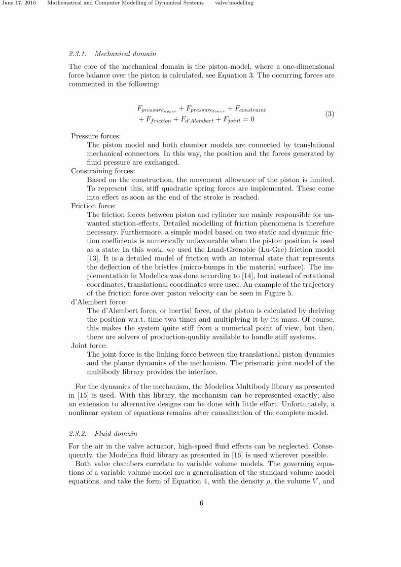
The core of the mechanical domain is the piston-model, where a one-dimensionalforce balance over the piston is calculated, see Equation 3. The occurring forces arecommented in the following:

Fpressureupper + Fpressurelower + Fconstraint

+ Ffriction + Fd′Alembert + Fjoint = 0(3)

Pressure forces:The piston model and both chamber models are connected by translationalmechanical connectors. In this way, the position and the forces generated byfluid pressure are exchanged.

Constraining forces:Based on the construction, the movement allowance of the piston is limited.To represent this, stiff quadratic spring forces are implemented. These comeinto effect as soon as the end of the stroke is reached.

Friction force:The friction forces between piston and cylinder are mainly responsible for un-wanted stiction-effects. Detailed modelling of friction phenomena is thereforenecessary. Furthermore, a simple model based on two static and dynamic fric-tion coefficients is numerically unfavourable when the piston position is usedas a state. In this work, we used the Lund-Grenoble (Lu-Gre) friction model[13]. It is a detailed model of friction with an internal state that representsthe deflection of the bristles (micro-bumps in the material surface). The im-plementation in Modelica was done according to [14], but instead of rotationalcoordinates, translational coordinates were used. An example of the trajectoryof the friction force over piston velocity can be seen in Figure 5.

d’Alembert force:The d’Alembert force, or inertial force, of the piston is calculated by derivingthe position w.r.t. time two times and multiplying it by its mass. Of course,this makes the system quite stiff from a numerical point of view, but then,there are solvers of production-quality available to handle stiff systems.

Joint force:The joint force is the linking force between the translational piston dynamicsand the planar dynamics of the mechanism. The prismatic joint model of themultibody library provides the interface.

For the dynamics of the mechanism, the Modelica Multibody library as presentedin [15] is used. With this library, the mechanism can be represented exactly; alsoan extension to alternative designs can be done with little effort. Unfortunately, anonlinear system of equations remains after causalization of the complete model.

2.3.2. Fluid domain

For the air in the valve actuator, high-speed fluid effects can be neglected. Conse-quently, the Modelica fluid library as presented in [16] is used wherever possible.

Both valve chambers correlate to variable volume models. The governing equa-tions of a variable volume model are a generalisation of the standard volume modelequations, and take the form of Equation 4, with the density ρ, the volume V , and

6


−0.015 −0.010 −0.005 0.000 0.005 0.010 0.015velocity [m/s]

−20

−10

0

10

20

fric

tion

forc

e[N

]

Figure 5. A trajectory (friction force w.r.t. velocity) of the Lund-Grenoble friction model

φ ∈ (1, u,x) representing mass, energy and substance balance respectively.

d

dt

(φ · ρ · V

)=∑

flow +∑

source (4)

In the case of the energy-balance, mechanical work on the cylindrical chambervolume now creates an interesting interaction between the fluid and mechanicaldomain. The implementation in Modelica can be seen in Listing 1. Note: TheactualStream-operator indicates the properties of the fluid crossing the port bound-ary. The noEvent-operator indicates that no state-events shall be generated whenthe fluid mass flow changes direction.

Listing 1 Extract of Modelica code for lower variable volume model

// translational mechanics interface

medium.p = - flange.f/area;

pos = flange.s;

volume = volume_0 + area*pos;

// mass balance

mass = volume*medium.d;

der(volume*medium.d) = sum(fluidPort.m_flow);

// energy balance (dU = dQ + dW)

der(volume*medium.d*medium.u) = sum(fluidPort[i].m_flow *

noEvent(actualStream(fluidPort[i].h_outflow)) for i in 1:ninf)

- medium.p*der(volume) + heatPort.Q_flow;

// substance balance

der(volume*medium.d*medium.Xi) = sum(fluidPort[i].m_flow * noEvent(

actualStream(fluidPort[i].Xi_outflow)) for i in 1:ninf);

7


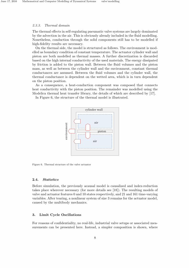
2.3.3. Thermal domain

The thermal effects in self-regulating pneumatic valve systems are largely dominatedby the advection in the air. This is obviously already included in the fluid modelling.Nonetheless, conduction through the solid components still has to be modelled ifhigh-fidelity results are necessary.

On the thermal side, the model is structured as follows. The environment is mod-elled as boundary condition of constant temperature. The actuator cylinder wall andpiston are both modelled as thermal masses. A further discretization is discardedbased on the high internal conductivity of the used materials. The energy dissipatedby friction is added to the piston wall. Between the fluid volumes and the pistonmass, as well as between the cylinder wall and the environment, constant thermalconductances are assumed. Between the fluid volumes and the cylinder wall, thethermal conductance is dependent on the wetted area, which is in turn dependenton the piston position.

As a consequence, a heat-conduction component was composed that connectsheat conductivity with the piston position. The remainder was modelled using theModelica thermal heat transfer library, the details of which are described by [17].

In Figure 6, the structure of the thermal model is illustrated.

air

cylinder wall

en

vir

on

men

t air

piston

Figure 6. Thermal structure of the valve actuator

2.4. Statistics

Before simulation, the previously acausal model is causalized and index-reductiontakes place wherever necessary (for more details see [18]). The resulting models ofvalve and actuator features 0 and 10 states respectively, and 21 and 161 time-varyingvariables. After tearing, a nonlinear system of size 3 remains for the actuator model,caused by the multibody mechanics.

3. Limit Cycle Oscillations

For reasons of confidentiality, no real-life, industrial valve setups or associated mea-surements can be presented here. Instead, a simpler composition is shown, where

8


two valves are used to reduce the pressure in a pipe. The Modelica diagram of thecomposition can be seen in Figure 7. The pipe models are based on the gas dynamicslibrary as presented by [10]. Each pipe-component represents a pipe of 20 meterslength and a diameter of 0.1m, totalling at a length of 80 meters and a volume ofaround 0.63m3.

valve1

valve2

hydraulic actuator

hydraulic actuator

ramp

duration=20

oscillation

diagnosis

Figure 7. Modelica diagram of oscillation test case

As boundary conditions, the input pressure (left side) is set to 3 bars, while theright boundary is modelled as a quadratic resistance, normalized to a fluid velocityof 10 m

s at a pressure of 1 bar. The valve actuators are run in pneumatic-mode andset to regulate the downstream pressure to 2 and 1 bars respectively.

When the composite model is simulated, limit cycle oscillations occur. Theseare displayed in Figure 8. For both valves, the piston gets stuck at the outmostdeflection, until the restoring forces are high enough to overcome the friction forces.

0 2 4 6 8 10 12 140

5

10

15

20

25

30

Ang

le[d

eg]

valve1.Anglevalve2.Angle

0 2 4 6 8 10 12 14time [s]

0.5

1.0

1.5

2.0

2.5

3.0

3.5

Pre

ssur

e[P

a]

×105

valve1.p1valve1.p2valve2.p2

Figure 8. Results of oscillation test case

To demonstrate the influence of friction and pneumatic forces on the oscillations,the friction force and the volume of the cylinders were multiplied with a scaling pa-

9


rameter. A two-dimensional sweep of the quasi-steady-state amplitudes and periodsover both scaling-parameters is shown in Figure 9.

It can be seen that the oscillations are strongly dependent on both factors. Fur-thermore, the interaction between both factors can be visibly divided into threesections: for friction forces or cylinder volumes below a certain treshold, no oscilla-tion takes place, no matter how large the other scaling factor is. As long as bothfactors are relatively small, some interactions can be seen.

0.2 0.4 0.6 0.8 1.0normalized friction forces

0.6

0.8

1.0

1.2

1.4

1.6

1.8

2.0

norm

aliz

edcy

linde

rvo

lum

es

amplitude [Pa]

3.0E4

6.0E4

9.0E4

1.2E5

1.5E5

1.8E5

2.1E5

2.4E5

0.2 0.4 0.6 0.8 1.0normalized friction forces

0.6

0.8

1.0

1.2

1.4

1.6

1.8

2.0

norm

aliz

edcy

linde

rvo

lum

es

period [s]

0.5

1.0

1.5

2.0

2.5

3.0

3.5

4.0

Figure 9. Amplitude and Period of oscillations for scaled friction forces and cylinder volumes

4. Modeling and Control System Design

4.1. Introduction

The Modelica technology allows for an integrated development of both plant modeland control system. In the case at hand, control of electro-pneumatic valves is adifficult task: As demonstrated in Section 3, or in works like [19], valve oscillationsare mainly dominated by friction forces. This phenomenon is usually called stiction,a combination of the words ”stick” and ”friction”. The balancing of stiction withthe tools of control systems engineering is called ”stiction compensation”.

In literature, two main strategies are described regarding stiction compensation.The first strategy (the knocker) uses pulses of predefined length and intensity ontop of the regular control signal to overcome the stiction regime [20]. The other(dithering) superimposes the control signal with a high-frequency zero-mean signalto average-out the friction characteristic [21]. For self-regulating pneumatic valvesboth approaches are not suitable: the control signal has no direct influence on thevalve stem, instead it imposes a mass flow on one of the valve chambers. In thisway, the control signal is first-order filtered. Conventional stiction compensationstrategies require a high-frequency interaction between actuator and valve stem,which is therefore not possible.

4.2. Control-driven Modeling

In this work we propose an alternative workflow, which is tied into the modellingaspect of the controlled system. The main idea is to use the detailed model to find

10


the best combination of sensors and sensor-positions to robustly estimate the currentfriction force during the valve operation. Knowledge about the current friction forcecan in turn be used to compensate for stiction-effects.

The complete workflow is summarized in Figure 10 and executed as follows:

Modelling of valve without frictionFrom the complete actuator model, the friction force is multiplied by zero.Alternatively, the damping term Fv · v can remain, if necessary for stability.

Modelling of external controller interfaceNormally, autonomous models are used. To change this, the actuator modelis extended with an external input, governing the mass flow into the uppercylinder. Additionally, relevant measurements are output.

Build-up of simple system modelUsing frictionless valve models with external interfaces, the complete systemis modelled. Low order pipe models are preferable, if analytic control designapproaches like linear quadratic gaussian control are to be used later.

Linearization of system model around set-pointThe system model is simulated until a steady state is reached. Using thelinear systems as described in [22], the system is linearized and the resultingstate-space representation is exported.

Development of a controller for linearized modelUsing standard approaches like LQG or H∞, a MIMO-controller for the re-sulting system is designed.

Testing of controller on detailed model without frictionThe controller is tested on a the system model in Modelica. If the performanceis not satisfactory, another controller has to be designed.

Development of friction estimatorDuring the sticking-phase of the valve operation, the piston does not move butthe friction force does change over time. This force itself is not directly measur-able, but it can be estimated. Based on prior knowledge about which variablescan be measured, different estimators can be developed and compared insidethe Modelling context. Key for this estimation is the force balance over thepiston as described in Equation 3, where all terms apart from the frictionterm can be measured, calculated or are small during normal operation. Thefriction is then estimated as the missing term that brings the sum of forces tozero.

Development of friction compensatorAs soon as a suitable estimator is available, information about the currentfriction force during operation can be used to design a friction compensator.Since the friction force can now be considered in an isolated way, a relativelyhigh gain can be used to offset this force without compromising system levelstability. Another approach could be implemented by augmenting the input ofthe integral action of the main controller with an offset based on the estimatedfriction, alleviating a common cause of limit cycle oscillations at the cost of anon-zero steady state error. The detailed development of friction compensationschemes goes beyond the scope of this paper.

Integration of compensator into controllerOn the system level, a friction compensator is integrated into the MIMO-controller for each valve inside the system.

Testing of compensated controller on detailed model

11


The complete system including friction is tested, using the compensatedMIMO-controller. If the performance is not satisfactory, another approachfor friction compensation has to be used.

Model valve

without friction

build simple

system model

linearize model

around setpoint

model external

controller interface

find controller for

linearized model

develop friction

estimator

develop friction

compensator

integrate compensator

into controller

test controller

Success

test controller

Figure 10. Control system development strategy

5. Model Sensitivities

In this section, the sensitivity of simulation results is analysed. First, a suitable testsetup is presented. Then, the effect of physical parameters and solver options onthe results of this test model is presented.

5.1. Test Model

During model testing, it became apparent that the valve dynamics can be classifiedinto three categories, depending on the boundary conditions and parameterisationof the valve.

(1) In some cases, the overall dynamics were stable, which resulted in a steadystate system as soon as initialization effects died down.

(2) In some cases, the system showed a chaotic behavior.(3) In the other cases, the system dynamics exhibited stable limit cycles.

To find a quantifiable metric for model sensitivities, steady state-cases are not in-teresting, while chaotic cases make it difficult to quantify model differences. There-fore, we chose a setup including limit-cycles as test-case. Accordingly, the model

12


from Section 3 was used. It was simulated for 25 seconds and the final frequencyand amplitude of the output pressure of the first valve were used as a comparison-variable.

5.2. Solver Options

Reasonable solver settings can be suggested by the following simple heuristic: thetest model is simulated using a large solver tolerance and the values of oscillationamplitude and frequency are stored. The solver tolerance is then reduced and thesimulation is repeated. This continues until the values of oscillation amplitude andfrequency do not change anymore. The largest tolerance that results in this finalvalues is defined as the required solver tolerance.

We tested the following solvers: lsodar, dassl2, runge-kutta4, radau2a, esdirk23a,dopri45, sdirk34hw, cerk23 and cvode. As the model is quite stiff due to the frictiondynamics, only four of those were able to solve the system in an acceptable timespan. Those four (dassl, sdirk34hw, lsodar, cvode) were analysed as described. Theresults can be seen in Figure 11.

10-7 10-6 10-5 10-4 10-3

solver tolerance (cvode)

0

20000

40000

60000

80000

100000

amplitude [Pa]

simulation time: 90s

amplitude

frequency

0.00

0.15

0.30

0.45

0.60

frequency [1/s]

10-7 10-6 10-5 10-4 10-3

solver tolerance (dassl)

0

20000

40000

60000

80000

100000

amplitude [Pa]


amplitude

frequency

0.00

0.15

0.30

0.45

0.60

frequency [1/s]

10-7 10-6 10-5 10-4 10-3

solver tolerance (sdirk34hw)

0

20000

40000

60000

80000

100000

amplitude [Pa]


amplitude

frequency

0.00

0.15

0.30

0.45

0.60

frequency [1/s]

10-7 10-6 10-5 10-4 10-3

solver tolerance (lsodar)

0

20000

40000

60000

80000

100000

amplitude [Pa]


amplitude

frequency

0.00

0.15

0.30

0.45

0.60

frequency [1/s]

Figure 11. Sensitivities of solver parameters

Evidently, the required solver tolerance is smallest for cvode (1e-5) and largestfor dassl (3e-3). The required solver tolerance is the tolerance where the predictedamplitude matches the asymptotic amplitude. However, using all four solvers at

2Dassl is a native DAE-solver, but we used dassl as a regular ODE-solver, after preparing the equations as

described in Section 2.4.

13


their respective required tolerance values, cvode is still the fastest.One definition of model stiffness is the following: ”A model is stiff if the simulation

requires stiff solvers”. In that sense, the model is stiff, since all adequate solvers(dassl, sdirk34hw, lsodar, cvode) are as well.

5.3. Physical Parameters

To use the model for simulations, a set of physical parameters has to be defined.Most of them have a geometrical meaning and can simply be looked up from thespecifications. For accurate results, there are however three separate measurementsto be done. In the following sections, the necessary measurements are introducedand the sensitivity of simulation results to those parameters is investigated. Fromthose findings, suggestions regarding the necessary exactness of model parametersare made.

5.4. Friction

In the calculation of the piston-friction as appearing in Equation 3, the Lund-Grenoble (Lu-Gre) friction model [13] is used. In this model, the friction character-istics are defined by 6 constants. These have to be looked up in literature, based onthe material-pairing, or obtained from experiments if exact results are needed.

For each of those 6 parameters, we sweeped the parameter values one-by-one andsimulated the test model. All other parameters where fixed. The resulting valuesfor oscillation amplitude and frequency can be seen in Figure 12.

Obviously, it is not easy to interpret this Figure. The highly nonlinear frictionmodel introduces chaotic behavior into the system. This results in significant modeldifferences even for negligible parameter deviations.

However, it is still possible to derive meaningful conclusions from this data: thefirst two parameters, Fs and Fc, correspond to the static and sliding friction forcesin simpler friction models. It can be seen that the oscillation amplitude increaseswith Fs (the static friction) and decreases with Fc (the sliding friction). This makessense physically, as a large difference between both values increases the stick-slipeffect, which is the main reason for valve oscillations.

The second two parameters, vs and Fv, exhibit a treshold behavior, where theoscillations vanish for vs > 0.0038m/s or Fv < 90Ns/m. It is of course stronglyrecommended to repeat this analysis after measuring friction parameters, to see ifthe treshold values are near the measured values. If so, the validity of the modelwill be questionable. Apart from this treshold effect, the influence of Fv seems tobe small, while vs exhibits a medium influence on the resulting oscillations.

The last two parameters, σ0 and σ1, have a medium and low influence on theoscillations, respectively.

In summary, when using this model, accurate measurements should be applied forthe derivation of the friction parameters. σ1 seems to be the least important factor,while Fv only plays an important role if the value is near a certain treshold.

5.5. Aerodynamic Torque

The aerodynamic torque as described in Equation 2 is a function on the angle ofthe valve-disc. This function differs somewhat based on the geometry, but can often

14


15 20 25 30 35 40 45 50 55 60Fs

0

40000

80000

120000

160000

amplitude [Pa]

amplitude

frequency0.00

0.15

0.30

0.45

0.60

frequency

[1/s]

5 10 15 20 25 30Fc

0

40000

80000

120000

160000

amplitude [Pa]

amplitude

frequency0.00

0.15

0.30

0.45

0.60

frequency

[1/s]

0.0010 0.0015 0.0020 0.0025 0.0030 0.0035 0.0040vs

0

40000

80000

120000

160000

amplitude [Pa]

amplitude

frequency0.00

0.15

0.30

0.45

0.60

frequency

[1/s]

40 60 80 100 120 140 160 180 200Fv

0

40000

80000

120000

160000

amplitude [Pa]

amplitude

frequency0.000.150.300.450.60

frequency

[1/s]

1000000 1500000 2000000 2500000 3000000 3500000 4000000σ0

0

40000

80000

120000

160000

amplitude [Pa]

amplitude

frequency0.00

0.15

0.30

0.45

0.60

frequency

[1/s]

500 1000 1500 2000 2500 3000σ1

0

40000

80000

120000

160000

amplitude [Pa]

amplitude

frequency0.00

0.15

0.30

0.45

0.60

frequency

[1/s]

Figure 12. Sensitivities of friction parameters (reference values are marked)

be estimated by CFD-calculations.In this analysis, we modelled the effects of dimension- as well as shape-deviations

of this function.To get a feel for the influence of the dimension on the oscillation dynamics, we

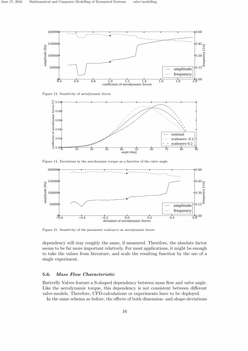
multiplied the computed torque with a scaling parameter. The result of a parametersweep can be seen in Figure 13.

Of course, not only the absolute factor of the aerodynamic torque can influencethe system dynamics, but also the shape of the valve angle-dependency. To analysethis, we extended the torque calculation with the term (1 + scaleaero ∗ sin(Angle ∗3 ∗ π/90)), resulting in an angle-dependent deviation. The resulting functions canbe seen in Figure 14 for values of the scaling parameter scaleaero of −0.2 and 0.2.The function for a vanishing value of the scaleaero is shown in black as a reference.

The result of a parameter sweep can be seen in Figure 15.To summarize, both deviations in dimension and in the shape of the valve angle-

dependency can have a large influence on the resulting dynamics if the measuredvalues are far off the actual values. However, one has to keep in mind that systematicerrors will be introduced much more easily, while the shape of the valve angle-

15


0.4 0.6 0.8 1.0 1.2 1.4 1.6 1.8 2.0coefficient of aerodynamic forces

0

50000

100000

150000

200000

amplitude [Pa]

amplitude

frequency0.00

0.15

0.30

0.45

0.60

frequency

[1/s]

Figure 13. Sensitivity of aerodynamic forces

0 10 20 30 40 50 60 70 80 90angle [deg]

0.00

0.02

0.04

0.06

0.08

0.10

coefficient of aerodyn

amic forces [1]

nominal

scaleaero -0.2

scaleaero 0.2

Figure 14. Deviations in the aerodynamic torque as a function of the valve angle

−0.6 −0.4 −0.2 0.0 0.2 0.4 0.6deviation of aerodynamic forces

0

50000

100000

150000

200000

amplitude [Pa]

amplitude

frequency0.00

0.15

0.30

0.45

0.60

frequency

[1/s]

Figure 15. Sensitivity of the parameter scaleaero on aerodynamic forces

dependency will stay roughly the same, if measured. Therefore, the absolute factorseems to be far more important relatively. For most applications, it might be enoughto take the values from literature, and scale the resulting function by the use of asingle experiment.

5.6. Mass Flow Characteristic

Butterfly Valves feature a S-shaped dependency between mass flow and valve angle.Like the aerodynamic torque, this dependency is not consistent between differentvalve-models. Therefore, CFD-calculations or experiments have to be deployed.

In the same schema as before, the effects of both dimension- and shape-deviations

16


on the system oscillations were analysed. The results are presented in Figure 16.

0.4 0.6 0.8 1.0 1.2 1.4 1.6 1.8 2.0coefficient of mass flo characteristic

0

50000

100000

150000

200000amplitude [Pa]

amplitude

frequency0.000.150.300.450.60

frequency [1/s]

−0.6 −0.4 −0.2 0.0 0.2 0.4 0.6deviation of mass flo characteristic

0

50000

100000

150000

200000

amplitude [Pa]

amplitude

frequency0.00

0.15

0.30

0.45

0.60

frequency [1/s]

Figure 16. Sensitivity of mass flow characteristic

For both dimensional and shape-variations, a treshold-effect is apparent. Even forsmall deviations in the wrong directions, the oscillations disappear instantly. Thislarge sensitivity points to a great accuracy which is needed during the measurementof this curves.

6. Dynamic interactions

The multi-domain nature of the presented model results in some interesting nonlin-ear transients. Two of them are presented in the following.

6.1. Aerodynamic Torque

The waterhammer effect is commonly known in pipeline operations. When a closingvalve is used to stop the flow of a heavy and fast fluid-mass, the residual momentumof the fluid generates a build-up of pressure upstream of the valve.

For self-regulating pneumatic valves, a similar effect can occur: let’s presupposethat the valve actuator closes the valve by a particular angle. The air mass upstreamof the valve is then decelerated as a result, while generating a temporary pressurebuild-up. This pressure-buildup in turn increases the aerodynamic torque on thevalve disk, closing the disk further and amplifying the effect.

In Figure 17, a test model is represented where a pressure-regulated pipe is sub-jected to a harmonic inlet pressure with increasing frequency. The model was sim-ulated with and without consideration of aerodynamic torque. The result of thesimulation can be seen in Figure 18. It is easily recognizable that the valve open-ing is smaller when taking aerodynamic torque in consideration, especially at thefrequencies that occur between 10 and 15 seconds.

17


hydraulic actuator

valve

prng_temp

2 s

mu=500

sigma=20

Figure 17. Aerodynamic Torque test model

0 5 10 15 200.80.91.01.11.21.31.41.51.61.7

Pre

ssur

e[P

a]

×107

valveWithoutAero.p1valveWithoutAero.p2valveWithAero.p1valveWithAero.p2

0 5 10 15 20time [s]

−1

0

1

2

3

4

5

6

Ang

le[d

eg]

×101

valveWithoutAero.AnglevalveWithAero.Angle

Figure 18. Transient effects of Aerodynamic Torque

6.2. Oscillatory heating

Generally, the environment of the valve has an ambient temperature different fromthe fluid temperature in the pipe. In a typical application area, aircraft bleed airsystems, the temperature difference can be around 500K. Also, heat conductionbetween environment and the valve chambers takes place. In the static case, thetemperature in the valve chamber will approach the ambient temperature after atime. However, in the case of valve movement, fluid mass is exchanged between thevalve chambers and the pipe. In this way, the resulting temperature of the valve isdependent on the amount of valve movement.

In Figure 19, the same test model as presented in Figure 17 is subjected to aconstant inlet pressure for 100 seconds, then subjected to an inlet pressure oscillatingwith a constant amplitude of 20 bars. The fluid inlet temperature is 500K, and theenvironment temperature is 370K. The inlet pressure oscillation results in significantvalve movements, and therefore a significant increase in air temperature inside thecylinder volumes.

18


80 100 120 140 160 180 2000.95

1.00

1.05

1.10

1.15

1.20

Pre

ssur

e[P

a]

×107

actuator.volumeUpper.medium.pactuator.volumeLower.medium.ppressureInlet.y

80 100 120 140 160 180 2003.603.653.703.753.803.853.903.954.004.05

Tem

pera

ture

[K]

×102

actuator.volumeUpper.medium.Tactuator.volumeLower.medium.T

80 100 120 140 160 180 200time [s]

2

3

4

5

6

7

8

9

Ang

le[d

eg]

×101

valve.Angle

Figure 19. Transient effects of oscillatory heating

7. Conclusion

Self-regulating pneumatic valves show a complex behavior, resulting in limit-cycleoscillations, if the overall system is not tuned satisfactorily. We present a detailedModelica model for this kind of valves. The model includes all relevant physicaleffects, representing the thermal, fluid, and mechanical domains. Simulation resultsexhibit the typical dynamical characteristics of self-regulating pneumatic valves.Subsequently, the model can be used to predict system performance in an earlydevelopment phase.

References

[1] A. Pollok and F. Casella, High-fidelity Modelling of Self-regulating Pneumatic Valves,in Proceedings of the 11th International Modelica Conference, 2015.

[2] M.S. Choudhury, S.L. Shah, N.F. Thornhill, and D.S. Shook, Automatic detection andquantification of stiction in control valves, Control Engineering Practice 14 (2006), pp.1395–1412.

[3] W. Bialowski, Dreams vs. reality: a view from both sides of the gap, Pulp and PaperCanada 94 (1993), pp. 19–27.

[4] L. Desborough and R. Miller, Increasing customer value of industrial control perfor-mance monitoring-Honeywell’s experience, in AIChE symposium series, 2002, pp. 169–189.

[5] P. Beater, Modeling and digital simulation of hydraulic systems in design and engi-neering education using Modelica and HyLib, in Modelica workshop, 2000, pp. 23–24.

[6] P. Beater and C. Clauß, Multidomain Systems: Pneumatic, Electronic and Mechanical

19


Subsystems of a Pneumatic Drive Modelled with Modelica, in Paper presented at the3rd International Modelica Conference, 2003.

[7] S.E. Pohl and M. Graf, Dynamic simulation of a free-piston linear alternator in mod-elica, in Modelica, 2005.

[8] A. Pujana-Arrese, J. Arenas, I. Retolaza, A. Martinez-Esnaola, and J. Landaluze, Mod-elling in Modelica of a pneumatic muscle: application to model an experimental set-up,in 21st European conference on modelling and simulation, ECMS, 2007, pp. 4–6.

[9] M. Sielemann, Device-oriented modeling and simulation in aircraft energy systems de-sign, Ph.D. diss., Hamburg University of Technology, 2012.

[10] M. Sielemann, High-Speed Compressible Flow and Gas Dynamics, in Proceedings of the9th International Modelica Conference, 2012.

[11] P.L. Roe, Approximate riemann solvers, parameter vectors, and difference schemes,Journal of computational physics 43 (1981), pp. 357–372.

[12] C. Solliec and F. Danbon, Aerodynamic torque acting on a butterfly valve. comparisonand choice of a torque coefficient, Journal of fluids engineering 121 (1999), pp. 914–917.

[13] C.C. De Wit, H. Olsson, K.J. Astrom, and P. Lischinsky, A new model for control ofsystems with friction, Automatic Control, IEEE Transactions on 40 (1995), pp. 419–425.

[14] M. Aberger and M. Otter, Modeling friction in Modelica with the Lund-Grenoble fric-tion model, in Proceedings of the 2nd International Modelica Conference, 2002.

[15] M. Otter, H. Elmqvist, and S.E. Mattsson, The new modelica multibody library, inProceedings of the 3rd International Modelica Conference, 2003.

[16] F. Casella, M. Otter, K. Proelss, C. Richter, and H. Tummescheit, The Modelica Fluidand Media library for modeling of incompressible and compressible thermo-fluid pipenetworks, in Proceedings of the Modelica Conference, 2006, pp. 631–640.

[17] M. Tiller, Introduction to physical modeling with Modelica, Springer Science & BusinessMedia, 2001.

[18] F.E. Cellier and E. Kofman, Continuous system simulation, Springer Science & Busi-ness Media, 2006.

[19] M.S. Choudhury, N.F. Thornhill, and S.L. Shah, Modelling valve stiction, Control en-gineering practice 13 (2005), pp. 641–658.

[20] T. Hagglund, A friction compensator for pneumatic control valves, Journal of processcontrol 12 (2002), pp. 897–904.

[21] K.J. Astrom, Control of systems with friction, Swedish Research Council for Eng.Science 759 (1995).

[22] M. Baur, M. Otter, and B. Thiele, Modelica libraries for linear control systems, inProceedings of 7th International Modelica Conference, Como, Italy, September, 2009,pp. 20–22.

20

Modelling and Simulation of Self-regulating Pneumatic Valves

Documents

Transcript of Modelling and Simulation of Self-regulating Pneumatic Valves