Modelling and Mapping of Coastal Inundation under …...collected along parts of the coastline of...
58
i Modelling and Mapping of Coastal Inundation under Future Sea Level Kathleen McInnes, Felix Lipkin, Julian O’Grady and Matthew Inman A report for Sydney Coastal Councils Group Cover Page - This cover page can be used with or without the pre-printed Flagships report covers Image Instructions A portrait or landscape image can be placed within this area (between the above red line and the grey strip below). There are two image positioning options: 1. The image to fill this area entirely. Click here to learn how. 2. The image floats anywhere within this area, ensuring it does not intrude above the red line or the blue strip. Click here to learn how If an image is not required, delete this instruction box then delete the red bordered box by clicking View then Header and Footer Collaborator Logos positioned here
Transcript of Modelling and Mapping of Coastal Inundation under …...collected along parts of the coastline of...
i
Modelling and Mapping of Coastal Inundation under Future Sea Level Kathleen McInnes, Felix Lipkin, Julian O’Grady and Matthew Inman A report for Sydney Coastal Councils Group
Cover Page - This cover page can be used with or without the pre-printed Flagships report covers Image Instructions A portrait or landscape image can be placed within this area (between the above red line and the grey strip below). There are two image positioning options: 1. The image to fill this area entirely. Click here to learn how. 2. The image floats anywhere within this area, ensuring it does not intrude above the red line or
the blue strip. Click here to learn how If an image is not required, delete this instruction box then delete the red bordered box by clicking View then Header and Footer
Collaborator Logos positioned here

[Insert ISBN or ISSN and Cataloguing-in-Publication (CIP) information here if required]
iii
Enquiries should be addressed to: Kathleen McInnes CSIRO Marine and Atmospheric Research
PMB #1, Aspendale, 3195
(03) 92394569
Dis tribution lis t [Insert name of person] [Insert copies received]
[Insert name of person] [Insert copies received]
[Insert name of person] [Insert copies received]
Copyright and Dis c la imer © 2011 CSIRO To the extent permitted by law, all rights are reserved and no part of this publication covered by copyright may be reproduced or copied in any form or by any means except with the written permission of CSIRO.
Important Dis c la imer CSIRO advises that the information contained in this publication comprises general statements based on scientific research. The reader is advised and needs to be aware that such information may be incomplete or unable to be used in any specific situation. No reliance or actions must therefore be made on that information without seeking prior expert professional, scientific and technical advice. To the extent permitted by law, CSIRO (including its employees and consultants) excludes all liability to any person for any consequences, including but not limited to all losses, damages, costs, expenses and any other compensation, arising directly or indirectly from using this publication (in part or in whole) and any information or material contained in it.
Contents
1. In troduction ....................................................................................................... 5
2. Background ....................................................................................................... 7 2.1 Contributions to Sea Level Extremes on the NSW Coast ......................................... 7 2.2 Methodology used in this study ............................................................................... 10 2.3 Extreme Sea Level Events from 1992 to 2009 ....................................................... 11
3. Dig ita l Eleva tion da ta ...................................................................................... 15 3.1 Data Sources .......................................................................................................... 15 3.2 Development of Consistent Gridded Data .............................................................. 19
4. Hydrodynamic and Model s e tup and res u lts ................................................. 21 4.1 Hydrodynamic Model ............................................................................................... 22 4.2 Event Description and Hydrodynamic Model Results ............................................. 22
4.2.1 Event 1: May 1997 .............................................................................................. 23 4.2.2 Event 2: June 1998 ............................................................................................. 26 4.2.3 Event 3: June 1999 ............................................................................................. 30 4.2.4 Event 4: July 2001 .............................................................................................. 33 4.2.5 Event 5: June 2007 ............................................................................................. 36
4.3 Wave Model Implementation .................................................................................. 39 4.4 Design Storm Construction and Sea Level Scenarios ............................................ 41 4.5 Design Storm results ............................................................................................... 42
5. Calcula tion of Inundation layers .................................................................... 46 5.1 Rationale ................................................................................................................. 47 5.2 Methodology ............................................................................................................ 47
6. Dis cus s ion and Conclus ion ........................................................................... 50
References ................................................................................................................ 52
Appendix a ................................................................................................................ 55
0BINTRODUCTION
Modelling and Mapping of Coastal Inundation under Future Sea Level • December 2011, Version 1.0 5
1. INTRODUCTION
Sea level increased over 1900 to 2009 at an average rate of 1.7 ± 0.2 mm/yr, with a statistically significant acceleration of 0.009 ± 0.004 mm/yr (Church and White 2011). Extreme sea levels analysed in global tide gauge data sets have also exhibited positive trends that are largely consistent with mean sea level trends (Woodworth and Blackman 2004; Menendez and Woodworth 2011). Rising sea levels will be felt most acutely during the coincidence of high tides and severe storm events when strong winds and lower-than-normal atmospheric pressure cause storm surges and high waves. Such events can lead to inundation of low lying coastal terrain, severe erosion and wave overtopping. Global averaged sea levels are projected to increase by 18 to 79 cm by 2090-2099 relative to 1980-1999 due to thermal expansion of the oceans, the melting of glaciers and ice sheets and an additional allowance for a potential rapid future increase in the dynamic ice sheet contribution to sea levels although it is emphasised that this contribution is highly uncertain and larger values cannot be excluded (IPCC 2007). Sea levels vary spatially across the globe due to variations in ocean temperature, salinity, ocean currents, winds and atmospheric pressure. Additionally, the rates of rise are also expected to vary spatially due to different regional changes in these contributions as well as changes in the gravitational potential of the ice sheets of Antarctica and Greenland and the Glaciers and Ice Caps as they lose mass (e.g. Church et al, 2011). An investigation of regional changes in sea level along the eastern Australian Coastline in Global Climate Models (GCMs) indicated that a strengthening of the East Australian Current may lead to relatively larger increases in sea level along the east coast of around 0.1 m by 2100 (McInnes et al, 2007). Recognising the potential for higher rates of rise along the east coast, the NSW Government has benchmarked expected sea-level rise to be 0.4m above the Australian Height Datum (AHD) by 2050 and 0.9m above AHD by 2100 (Coastal Risk Management Guide, 2010). Sea-level rise is anticipated to expose low-lying coastal areas to increasing inundation over the next century. This has prompted considerable focus by all levels of government over recent years on the evaluation of inundation risk for coastal regions. The Department of Climate Change, through its first pass National Coastal Vulnerability Program investigated coastal vulnerability at the national level due to potential shoreline change and vulnerability to inundation (see http://www.climatechange.gov.au/publications). The Future Coasts Program in Victoria, has undertaken a LiDAR survey of the entire state’s coastline including both terrestrial and shallow bathymetric components (http://www.climatechange.vic.gov.au/adapting-to-climate-change/future-coasts/digital-elevation-models-and-data. It also commissioned a modelling study to investigate extreme sea levels along the Victorian coast under present and future climate conditions (McInnes et al., 2009a, b, c). As part of the Climate Futures for Tasmania program LiDAR data has also been collected along parts of the coastline of Tasmania and a modelling study has been undertaken to establish extreme water levels along that coastline (McInnes et al, 2011). Previous studies carried out in support of these programs have focussed on quantifying the extreme sea levels associated with particular return period such as the 1 in 100 year water level (e.g. McInnes et al, 2009; McInnes et al, 2011). To these levels, scenarios of future sea level rise are added and the coastal land at risk of inundation has been evaluated. The method used
0BINTRODUCTION
6 Modelling and Mapping of Coastal Inundation under Future Sea Level • December 2011, Version 1.0]
for evaluating inundation is the ‘bathtub fill’ method (e.g. Department of Climate Change, 2009; Mount et al, 2010; McInnes et al, 2011a).
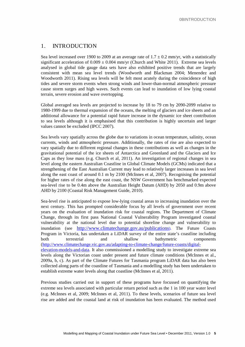
The present study focuses on the evaluation of extreme sea level inundation along the Sydney coastal and estuarine regions spanned by the Sydney Coastal Councils Group (see Figure 1) under current and future sea level rise conditions. Dynamical models of the coastal ocean are used to represent the physical contributions to extreme sea levels as well as capture the spatial variations in extreme sea levels that arise along the coast due the varying influences of the different physical processes. A novel aspect of this study is that in addition to the commonly considered contributions to extreme sea level from tides and storm surge, this study also considers the contribution of waves to elevated sea levels during the storm events. The evaluation of inundation layers is achieved using the ‘bathtub fill’ method to take advantage of the greater accuracy of high resolution terrestrial LiDAR data across the Sydney Coastal Councils Region.
Figure 1: The shaded area shows the region covered by the Sydney Coastal Councils Group.
Hornsby
Pittwater
Warringah
WilloughbyManly
Sutherland
RockdaleBotany Randwick
WoollahraWaverley
SydneyLeichhardtSouth Sydney
North Sydney Mosman
Hornsby
Pittwater
Warringah
WilloughbyManly
Sutherland
RockdaleBotany Randwick
WoollahraWaverley
SydneyLeichhardtSouth Sydney
North Sydney Mosman
1BBACKGROUND
Modelling and Mapping of Coastal Inundation under Future Sea Level • December 2011, Version 1.0 7
2. BACKGROUND
In this section, the contributions to extreme sea levels along the NSW coast are described. The approach used for modelling extreme sea levels is discussed. Finally an analysis of extreme sea level events at Sydney from 1992 to 2009 is presented along with the selection of a small number of events for subsequent modelling.
2.1 Contributions to Sea Leve l Extremes on the NSW Coas t
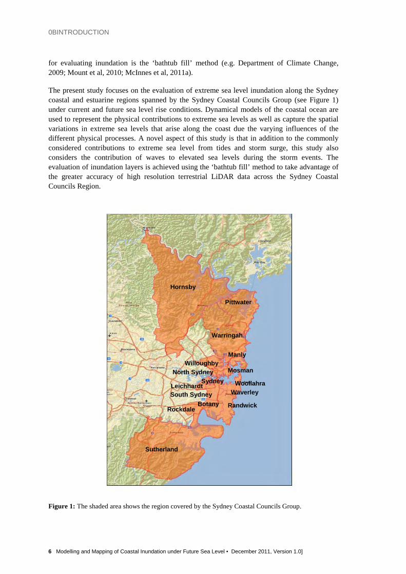
Coastal sea levels vary on different timescales due to different physical forcing. Astronomical tides cause sea level variations on a range of timescales ranging from sub-daily (high and low tides), through fortnightly (spring and neap tides) to annual and longer timescales. Low pressure and strong winds associated with severe weather events can cause fluctuations in coastal sea levels which are commonly called storm surges. Associated with storm surges are wind driven waves which can also contribute to elevated sea levels through wave setup. Variations in mean sea level also occur on seasonal and inter-annual time scales, the most significant contribution to inter-annual variations in sea levels around Australia being due to the El Nino Southern Oscillation. Superimposed on these variations are the long term increases in sea level due to global warming. These various contributions are illustrated in Figure 2. Figure 2: Schematic illustrating the contributions to coastal sea levels. Extreme sea levels comprise some combination of storm surge and astronomical tide, often referred to as a storm tide. Note that a stormtide can comprise a large surge in combination with a small or even negative tide or a moderate surge in combination with a particularly high tide. Sea levels may be further amplified at the coast due to wave breaking processes such as wave setup and run-up. The tidal range has along the NSW coast has a weak south to north gradient with the tidal range in northern NSW approximately 0.2 m greater than in southern NSW (MHL, 2011). There is a semi-annual variation in spring tides with the maximum in the spring tidal range occurring around the winter and summer solstices. The solstitial spring tidal range at the
1BBACKGROUND
8 Modelling and Mapping of Coastal Inundation under Future Sea Level • December 2011, Version 1.0]
Sydney tide gauge at Middle head is 1.829 m compared to the mean spring tidal range of 1.241 m (MHL, 2008). Non-tidal contributions to sea levels occur through a range of processes, the most significant being local severe weather forcing. The most common weather system to contribute to extreme sea levels in the Sydney region was found to be east coast low pressure systems (McInnes and Hubbert, 2001). Falling atmospheric pressure contributes to elevated sea levels due to the inverse barometer effect, where sea levels increase by approximately 1 cm for every hPa fall in pressure relative to ambient pressure conditions. Associated with the falling pressure are strong winds, which further elevate coastal sea levels. This can occur due to wind setup or current setup. Wind setup occurs where wind stress caused by onshore winds produces a gradient in ocean levels, which is maintained in the presence of a coastal boundary. The magnitude of wind setup is related to the depth and width of the continental shelf whereby higher sea levels from wind setup occur over wide and shallow continental shelves. In the absence of a coastal boundary to block flow, such as is the case when the wind blows obliquely toward the coast or along shore, the wind stress induces a longshore current which, if sustained for several days, can become deflected to the left in the Southern Hemisphere due to the Coriolis force. If the deflected current encounters a coastal boundary then elevated coastal levels occur. On the NSW coast, this situation would arise from sustained winds from the south. This is often referred to as current setup. The combination of the inverse barometer and wind stress contributions to elevated sea levels is called a storm surge. The one year annual recurrence of non-tidal component of sea levels has been estimated at tide gauges along the NSW coast (MHL, 2011). With the exception of gauges that are affected additionally by flood waters, these values are similar in value along the NSW coast with values in the north that are slightly higher than the south. At the Fort Denison and Sydney tide gauges, the values are approximately 0.42m. In other words, sea levels exceed the predicted tide by 0.42m, on average, once every year. Waves also affect coastal sea levels on the open coast. Waves may be due to short period storm waves during strong wind conditions, or long period swell waves, which have been generated by more distant storm systems and propagate through the deep ocean with little loss of wave energy. Two aspects of wave breaking are important in relation to coastal sea levels. The cumulative effect of wave breaking in the surf zone leads to a shoreward momentum transfer, and consequent elevation in coastal sea levels known as wave setup. Typically, wave setup is at the coast is considered to reach between 15 and 20% of the incident rms wave height (WMO, 1988). The contribution to coastal sea levels due to storms from wave setup has been estimated to be 0.7-1.5 m on the NSW coast (NSW Govt, 1990). Wave runup is the additional vertical distance that the water reaches due to the breaking of individual waves at the coast. Although wave runup is transitory and therefore not a contributor to the ‘still water levels’, it has been estimated to reach an elevation of 4.0-8.0 m higher than the still water level attained by the combination of astronomical tides, storm surge and wave setup (NSW Govt, 1990). Waves breaking processes are mainly of concern on the open coastline. Estuaries and harbours are generally sheltered from the additional sea level contributions due to wave setup or runup although local wave breaking within a harbour may have some effect for winds from particular directions (Watson and Lord, 2008). Wave height return periods have been estimated for the Sydney wave rider buoy by Shand et al, (2011). Although locally occurring weather events are the main cause of elevated coastal waters through the generation of storm surges, remote forcing along the southern coastline can also generate elevated sea levels. These elevated sea levels, once generated, can propagate along the
1BBACKGROUND
Modelling and Mapping of Coastal Inundation under Future Sea Level • December 2011, Version 1.0 9
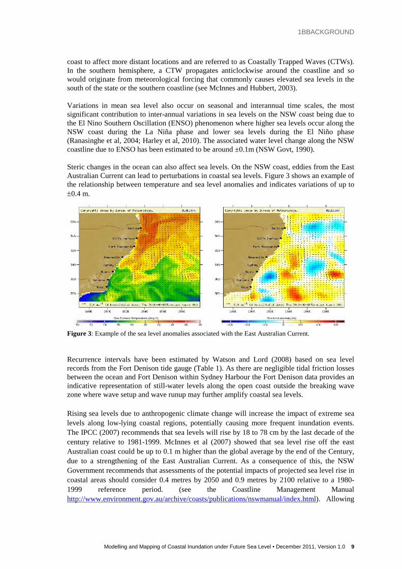
coast to affect more distant locations and are referred to as Coastally Trapped Waves (CTWs). In the southern hemisphere, a CTW propagates anticlockwise around the coastline and so would originate from meteorological forcing that commonly causes elevated sea levels in the south of the state or the southern coastline (see McInnes and Hubbert, 2003). Variations in mean sea level also occur on seasonal and interannual time scales, the most significant contribution to inter-annual variations in sea levels on the NSW coast being due to the El Nino Southern Oscillation (ENSO) phenomenon where higher sea levels occur along the NSW coast during the La Niña phase and lower sea levels during the El Niño phase (Ranasinghe et al, 2004; Harley et al, 2010). The associated water level change along the NSW coastline due to ENSO has been estimated to be around ±0.1m (NSW Govt, 1990). Steric changes in the ocean can also affect sea levels. On the NSW coast, eddies from the East Australian Current can lead to perturbations in coastal sea levels. Figure 3 shows an example of the relationship between temperature and sea level anomalies and indicates variations of up to ±0.4 m. Figure 3: Example of the sea level anomalies associated with the East Australian Current. Recurrence intervals have been estimated by Watson and Lord (2008) based on sea level records from the Fort Denison tide gauge (Table 1). As there are negligible tidal friction losses between the ocean and Fort Denison within Sydney Harbour the Fort Denison data provides an indicative representation of still-water levels along the open coast outside the breaking wave zone where wave setup and wave runup may further amplify coastal sea levels. Rising sea levels due to anthropogenic climate change will increase the impact of extreme sea levels along low-lying coastal regions, potentially causing more frequent inundation events. The IPCC (2007) recommends that sea levels will rise by 18 to 78 cm by the last decade of the century relative to 1981-1999. McInnes et al (2007) showed that sea level rise off the east Australian coast could be up to 0.1 m higher than the global average by the end of the Century, due to a strengthening of the East Australian Current. As a consequence of this, the NSW Government recommends that assessments of the potential impacts of projected sea level rise in coastal areas should consider 0.4 metres by 2050 and 0.9 metres by 2100 relative to a 1980-1999 reference period. (see the Coastline Management Manual http://www.environment.gov.au/archive/coasts/publications/nswmanual/index.html). Allowing

1BBACKGROUND
10 Modelling and Mapping of Coastal Inundation under Future Sea Level • December 2011, Version 1.0]
for the different reference periods between the sea level rise estimates and the return levels reported in Table 1, Table 4.1 lists the relevant extreme sea level values at Fort Denison that are to be considered in the extreme sea level modelling. Table 1: Sydney Harbour design still water levels relative to Indian Springs Low Water Datum (ISLW) and Australian Height Datum (AHD), which is 0.925 m lower than ISLW. (source Watson and Lord, 2008; Coastal Risk Management Guide, 2010) ARI (years)
Maximum Sea Level 2010 2050 2100 m ISLW m AHD m AHD m AHD
0.02 1.89 0.97 1.31 1.81 0.05 1.97 1.05 1.39 1.89 0.10 2.02 1.1 1.44 1.94 1 2.16 1.24 1.58 2.08 5 2.24 1.32 1.66 2.16 10 2.27 1.35 1.69 2.19 50 2.34 1.42 1.75 2.25 100 2.36 1.44 1.78 2.28
2.2 Methodology us ed in th is s tudy
The focus of this study is the development of maps showing the inundation that arises from contribution of storm surges and astronomical tides to extreme sea levels which are referred to as storm tides. Wave breaking can further elevate sea levels through wave setup, and this process is considered in the present study. However, other processes that can further elevate sea levels such as ENSO, CTW, thermodynamic contributions related to eddy activity from the EAC are not considered in this study. Additionally, the transient sea level activity associated with wave runup is also not considered in this study, although a flexible framework for assessing coastal inundation has been adopted so that information on wave setup could be incorporated in the future. The approach adopted in this study is to use a ‘design storm approach’. In this, an actual storm event is used to simulate sea levels along the coast due to tides, storm surge and wave setup. The objective is to select an event that is driven primarily by a severe weather event, is well represented by the modelling system. Features of the selected event such as wind speed, or the phasing of the storm system with tides can then be modified so that the actual sea levels simulated by the event match those associated with particular recurrence intervals. In this study, the aim is to construct an event that produces the sea levels associated with a 1-in-1 year event and a 1-in -100 year event. For this purpose, the established return periods for Fort Denison, reproduced in Table 1, are used to calibrate an actual storm. The reason for adopting this modelling approach for simulating coastal sea levels rather than using a constant return level
1BBACKGROUND
Modelling and Mapping of Coastal Inundation under Future Sea Level • December 2011, Version 1.0 11
from Table 1 as a basis for inundation modelling is that the various contributions to sea levels from processes such as wave breaking and wind setup will not lead to constant sea levels throughout the Sydney Coastal Councils region. For example, for a given value of sea level at Fort Denison inside Sydney Harbour, sea levels along the coastal beaches can be expected to be higher due to the effects of wave breaking. Also, the effect of wind stress will not be uniform and will have a greater effect on windward oriented coastlines. These variations can be captured by taking a dynamic modelling approach. As well as this, for the consideration of future sea level rise, the dynamic modelling approach will represent any non-linear responses to the higher sea levels that arise. For example, wave breaking is affected by depth and bathymetric profiles in the near shore region.
To identify events that will be suitable for use in the design storm approach, extreme events over the recent observational period are characterised in terms of their total sea level, residual sea level and waves. A selection of events that are severe on the basis of these criteria are then selected for modelling and further analysis in Chapter 4. From this the required forcing conditions are assembled, that when modelled, reproduce sea levels at Fort Denison that match the 1-in-1 year and 1-in-100 year levels of 1.24 and 1.44 m respectively. These events will then form the basis of the sea level modelling to underpin the inundation analysis carried out in Chapter 5.
2.3 Extreme Sea Leve l Events from 1992 to 2009
Extreme sea level events in Sydney have been analysed in a number of previous studies. Watson and Lord (2008) analysed total water level at Fort Denison (e.g. Watson and Lord, 2008) and Modra, (2011) publishes highest recorded water levels and anomalies based on data from the Fort Denison tide gauge over the period 1915-2007. Extreme high waves have been analysed (e.g. Shand et al, 2011) using data from the Sydney wave rider buoy situated off the Sydney coast at approximately 33.78º and 151.42º. However for the purposes of testing model performance and selecting events suitable to use as a basis for the inundation modelling, it is necessary to select potential extreme sea level events over the past two decades over which time wave observations and high resolution atmospheric reanalysis products are available to provide spatially and temporally varying fields of 10 m winds and mean sea level pressure to force hydrodynamic and wave models. Therefore, directional wave data from the Sydney wave rider buoy over the 1992-2010 period, and tide gauge data from Fort Denison over this same period was used as a basis for this analysis.
Hourly values of the wave parameters such as significant wave height (Hs), peak wave period (Tp1) and wave direction (Wd), total sea levels (ζtot) and detided sea level residuals (ζres ) were assembled and missing values of 6 hours or less were filled using linear interpolation. Extreme total sea level events were identified as having commenced when values exceeded 1.1 m and ending when values dropped below 1.1 m for at least 24 hours. Residual sea level events were identified as having commenced when values of residual sea levels exceeded 0.15 m and ending when values dropped below 0.15 m for at least 24 hours. Significant wave height events were identified as having commenced when values exceeded 3 m and ending when values dropped below 3 m for at least 12 hours. Using these thresholds over the 18 years of records, a total of 66 events for ζtot, 254 events for ζres and 399 events for Hs were identified. The top 20 events for ζtot , ζres and Hs are summarised in Tables 2 – 4. In many cases, events are found be extreme on more than one criteria.

1BBACKGROUND
12 Modelling and Mapping of Coastal Inundation under Future Sea Level • December 2011, Version 1.0]
Table 2: Top 20 events ranked in order of total sea level, ζtot. Values of other parameters are given at the time of the peak in ζtot where Hs is significant wave height; ζtid is predicted tide; ζ
res = ζtot - ζtid is residual sea level; Wd is average wave direction and Tp is significant wave period. An event is defined as commencing when ζ tot exceeds 1.1m and finishing when ζ tot remains below 1.1 m for at least 24 hours. Sea levels are AHD, times are in UTC and durations have been rounded to the nearest day. Date/time of Peak
ζtot (m) Rank
Hs (m) Rank
ζtid (m) Rank
ζres (m) Rank
Wd (deg)
Tp (s) Duration
19/08/2001 10:00 1.34 1 NA 59 1.06 34 0.28 3 NA NA 18-21/08/2001
14/06/1999 11:00 1.29 2 1.29 42 1.13 3 0.16 17 150 11.1 12-16/06/1999
14/06/2007 10:00 1.29 3 2.32 16 1.05 37 0.24 8 159 11.5 14-16/06/2007
30/07/1992 11:00 1.28 4 0.94 50 1.09 24 0.19 13 157 13.3 29-30/07/1992
23/06/1998 10:00 1.27 5 1.88 24 1.02 46 0.25 5 163 12.5 23-24/06/1998
15/06/2003 11:00 1.26 6 NA 60 1.11 9 0.14 21 NA NA 14-17/06/2003
13/07/1995 11:00 1.26 7 0.71 57 1.11 11 0.15 20 160 14.8 12-13/07/1995
31/12/2001 23:00 1.26 8 0.80 54 1.01 50 0.25 6 142 8.8 29/12/01-3/1/02
22/07/2009 11:00 1.25 9 0.87 52 1.10 18 0.15 18 155 16.0 21-23/07/2009
13/12/2008 23:00 1.24 10 NA 61 1.12 5 0.12 30 NA NA 12-15/12/2008
7/08/1998 10:00 1.23 11 3.25 10 0.90 66 0.33 1 132 10.8 7-7/08/1998
25/05/1994 10:00 1.23 12 0.55 58 1.11 12 0.12 31 49 4.3 25-26/05/1994
12/06/2002 11:00 1.22 13 1.03 46 0.95 62 0.27 4 163 12.2 12-13/06/2002
22/12/1995 23:00 1.22 14 2.06 21 1.11 13 0.11 33 167 10.5 21-23/12/1995
25/06/1998 11:00 1.21 15 1.72 28 1.01 48 0.20 11 170 10.5 25-25/06/1998
2/06/2000 10:00 1.21 16 3.83 6 1.07 30 0.14 23 171 12.2 1-3/06/2000
13/06/1995 10:00 1.21 17 2.13 19 1.13 4 0.07 47 162 10.5 12-14/06/1995
25/05/1998 10:00 1.20 18 3.65 7 1.06 35 0.14 24 172 10.0 25-25/05/1998
30/06/2000 9:00 1.20 19 5.89 3 1.02 47 0.18 14 174 12.2 30-01/06/2000
7/11/1994 1:00 1.20 20 NA 62 0.95 61 0.25 7 NA NA 4-7/11/1994
These events are used to select a subset of events suitable for modelling with hydrodynamic and wave models in Chapter 4. The modelling of events with the hydrodynamic model will serve two purposes. Firstly, analysing the synoptic circumstances surrounding these events and simulating the oceanic response to the atmospheric conditions with the hydrodynamic model will validate the model performance. Secondly, this modelling will allow the identification of events that, possibly because they are not well simulated by the hydrodynamic model, are caused in part by additional processes and forcing that are not taken into account by the hydrodynamic model used. These may include, for example, sea level anomalies due to CTWs that are generated by severe weather systems outside the region modelled in this study, or thermodynamic contributions to sea level perturbations that may arise from eddy activity from
1BBACKGROUND
Modelling and Mapping of Coastal Inundation under Future Sea Level • December 2011, Version 1.0 13
the East Australian Current. A subset of five events selected on the basis of high waves, high residuals and or high total sea levels are listed in Table 5. In most cases they represent the highest events listed in Tables 2-4 with the exception of the high total water level events which were ranked 2nd and 4th highest. In this case, the 1st and 3rd highest events were not considered because Sydney wave buoy data was not available.
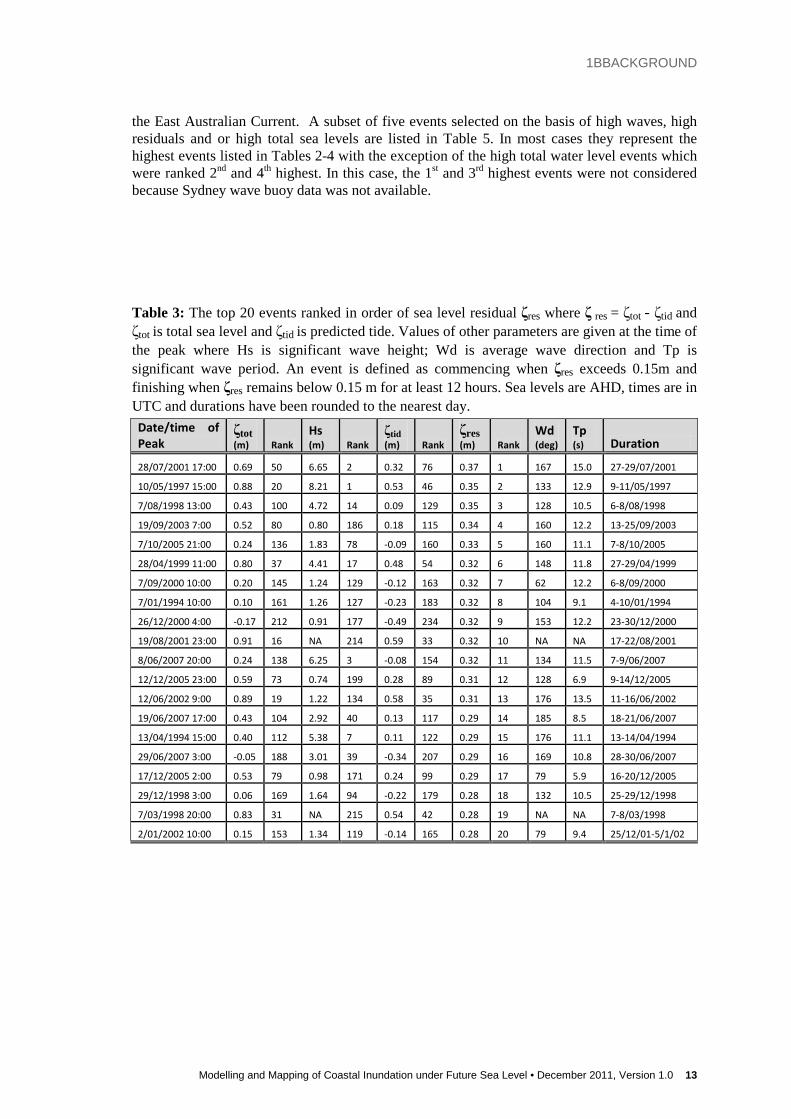
Table 3: The top 20 events ranked in order of sea level residual ζres where ζ res = ζtot - ζtid and ζtot is total sea level and ζtid is predicted tide. Values of other parameters are given at the time of the peak where Hs is significant wave height; Wd is average wave direction and Tp is significant wave period. An event is defined as commencing when ζres exceeds 0.15m and finishing when ζres remains below 0.15 m for at least 12 hours. Sea levels are AHD, times are in UTC and durations have been rounded to the nearest day. Date/time of Peak
ζtot (m) Rank
Hs (m) Rank
ζtid (m) Rank
ζres (m) Rank
Wd (deg)
Tp (s) Duration
28/07/2001 17:00 0.69 50 6.65 2 0.32 76 0.37 1 167 15.0 27-29/07/2001
10/05/1997 15:00 0.88 20 8.21 1 0.53 46 0.35 2 133 12.9 9-11/05/1997
7/08/1998 13:00 0.43 100 4.72 14 0.09 129 0.35 3 128 10.5 6-8/08/1998
19/09/2003 7:00 0.52 80 0.80 186 0.18 115 0.34 4 160 12.2 13-25/09/2003
7/10/2005 21:00 0.24 136 1.83 78 -0.09 160 0.33 5 160 11.1 7-8/10/2005
28/04/1999 11:00 0.80 37 4.41 17 0.48 54 0.32 6 148 11.8 27-29/04/1999
7/09/2000 10:00 0.20 145 1.24 129 -0.12 163 0.32 7 62 12.2 6-8/09/2000
7/01/1994 10:00 0.10 161 1.26 127 -0.23 183 0.32 8 104 9.1 4-10/01/1994
26/12/2000 4:00 -0.17 212 0.91 177 -0.49 234 0.32 9 153 12.2 23-30/12/2000
19/08/2001 23:00 0.91 16 NA 214 0.59 33 0.32 10 NA NA 17-22/08/2001
8/06/2007 20:00 0.24 138 6.25 3 -0.08 154 0.32 11 134 11.5 7-9/06/2007
12/12/2005 23:00 0.59 73 0.74 199 0.28 89 0.31 12 128 6.9 9-14/12/2005
12/06/2002 9:00 0.89 19 1.22 134 0.58 35 0.31 13 176 13.5 11-16/06/2002
19/06/2007 17:00 0.43 104 2.92 40 0.13 117 0.29 14 185 8.5 18-21/06/2007
13/04/1994 15:00 0.40 112 5.38 7 0.11 122 0.29 15 176 11.1 13-14/04/1994
29/06/2007 3:00 -0.05 188 3.01 39 -0.34 207 0.29 16 169 10.8 28-30/06/2007
17/12/2005 2:00 0.53 79 0.98 171 0.24 99 0.29 17 79 5.9 16-20/12/2005
29/12/1998 3:00 0.06 169 1.64 94 -0.22 179 0.28 18 132 10.5 25-29/12/1998
7/03/1998 20:00 0.83 31 NA 215 0.54 42 0.28 19 NA NA 7-8/03/1998
2/01/2002 10:00 0.15 153 1.34 119 -0.14 165 0.28 20 79 9.4 25/12/01-5/1/02

1BBACKGROUND
14 Modelling and Mapping of Coastal Inundation under Future Sea Level • December 2011, Version 1.0]
Table 4: The top 20 events ranked in order of significant wave height Hs. Values of other parameters are given at the time of the peak in Hs where ζtot is total sea level, ζres = ζtot - ζtid and ζtid is predicted tide. Values of other parameters are given at the time of the peak where Hs is significant wave height; Wd is average wave direction and Tp is significant wave period. An event is defined as commencing when ζres exceeds 0.15m and finishing when ζ res remains below 0.15 m for at least 12 hours. Sea levels are AHD, times are in UTC and durations have been rounded to the nearest day. Date/time of Peak
ζtot (m) Rank
Hs (m) Rank
ζtid (m) Rank
ζres (m) Rank
Wd (deg)
Tp (s) Duration
10/05/1997 16:00 0.58 50 8.43 1 0.24 135 0.34 1 151 12.8 9-12/05/1997
8/06/2007 16:00 0.92 4 6.87 2 0.65 26 0.27 3 135 10.8 7-10/06/2007
22/03/2005 18:00 0.49 74 6.61 3 0.27 126 0.22 9 139 12.2 21-24/03/2005
19/07/2007 11:00 0.44 90 6.52 4 0.26 128 0.18 23 158 12.9 18-20/07/2007
3/06/2006 9:00 0.00 206 6.46 5 -0.10 236 0.11 70 173 13.5 2-4/06/2006
29/06/2002 5:00 -0.01 212 6.23 6 -0.09 230 0.08 105 164 13.5 28-30/06/2002
20/11/2001 23:00 0.33 119 6.22 7 0.18 154 0.15 40 145 11.1 18-22/11/2001
11/06/2006 7:00 0.45 84 6.21 8 0.38 89 0.08 109 183 12.2 10-12/06/2006
10/07/2005 6:00 -0.08 233 6.20 9 -0.31 299 0.24 6 160 12.2 10-10/07/2005
23/04/1999 5:00 0.45 85 6.18 10 0.35 101 0.10 78 98 15.4 21-25/04/1999
8/10/2009 0.00 0.88 9 6.17 11 0.75 12 0.13 48 183 13.8 7-9/10/2009
30/06/2000 8:00 1.10 1 6.13 12 0.92 3 0.18 25 177 11.1 29/06-02/07/2000
30/08/1996 17:00 -0.63 385 6.09 13 -0.73 398 0.11 67 136 11.1 30-31/08/1996
22/08/2008 21:00 -0.39 334 6.08 14 -0.45 340 0.06 140 179 11.5 22-24/08/2008
14/07/1999 14:00 0.51 67 6.07 15 0.40 83 0.11 69 117 11.8 13-16/07/1999
15/06/2007 22:00 0.50 73 6.03 16 0.31 113 0.19 20 128 10.3 15-18/06/2007
31/03/2009 2:00 0.38 104 5.91 17 0.37 93 0.01 221 100 11.5 30/03-2/4/2009
15/11/2005 14:00 -0.24 282 5.85 18 -0.40 319 0.16 36 183 11.1 15-16/11/2005
15/08/2002 16:00 0.34 116 5.84 19 0.34 106 0.00 233 139 12.2 14-17/08/2002
28/10/2004 9:00 0.30 124 5.81 20 0.35 102 -0.05 309 169 15.0 27-29/10/2004
Table 5: The events selected for modelling. The values of ζtot , Hs, ζres and ζtid are the maximum values to have occurred throughout the event duration as distinct from the values in Tables 2-4 which show the value of all variables at the time of the peak in the ranked variable.
Event Number Event Duration
ζtot (m)
Hs (m)
ζres (m)
ζtid (m) Comments
1 10/05/1997 - 12/05/1997 1.16 8.43 0.35 0.83 high waves and residual
2 23/06/1998 - 23/06/1998 1.27 2.47 0.28 1.02 high total sea level
3 13/06/1999 - 15/06/1999 1.29 2.35 0.18 1.13 high total sea level
4 27/07/2001 - 30/07/2001 0.88 6.97 0.37 0.61 high residual
5 7/06/2007 - 10/06/2007 0.92 6.87 0.32 0.71 high waves
2BDIGITAL ELEVATION DATA
Modelling and Mapping of Coastal Inundation under Future Sea Level • December 2011, Version 1.0 15
3. DIGITAL ELEVATION DATA
Topographic and bathymetric data in the form of a digital elevation model is a fundamental parameter of the physical modelling that is described in Chapter 4. As the resolution, accuracy and extent of the digital elevation data that each specific model requires varies, it was evaluated that a single seamless topographic/bathymetric elevation grid of the highest resolution possible would generate a suitable level of consistency from which to interpolate to each of the model grids. This section provides an overview of the datasets and methods used to create a seamless topographic/bathmetytric elevation grid from multiple data sources.
3.1 Data Sources
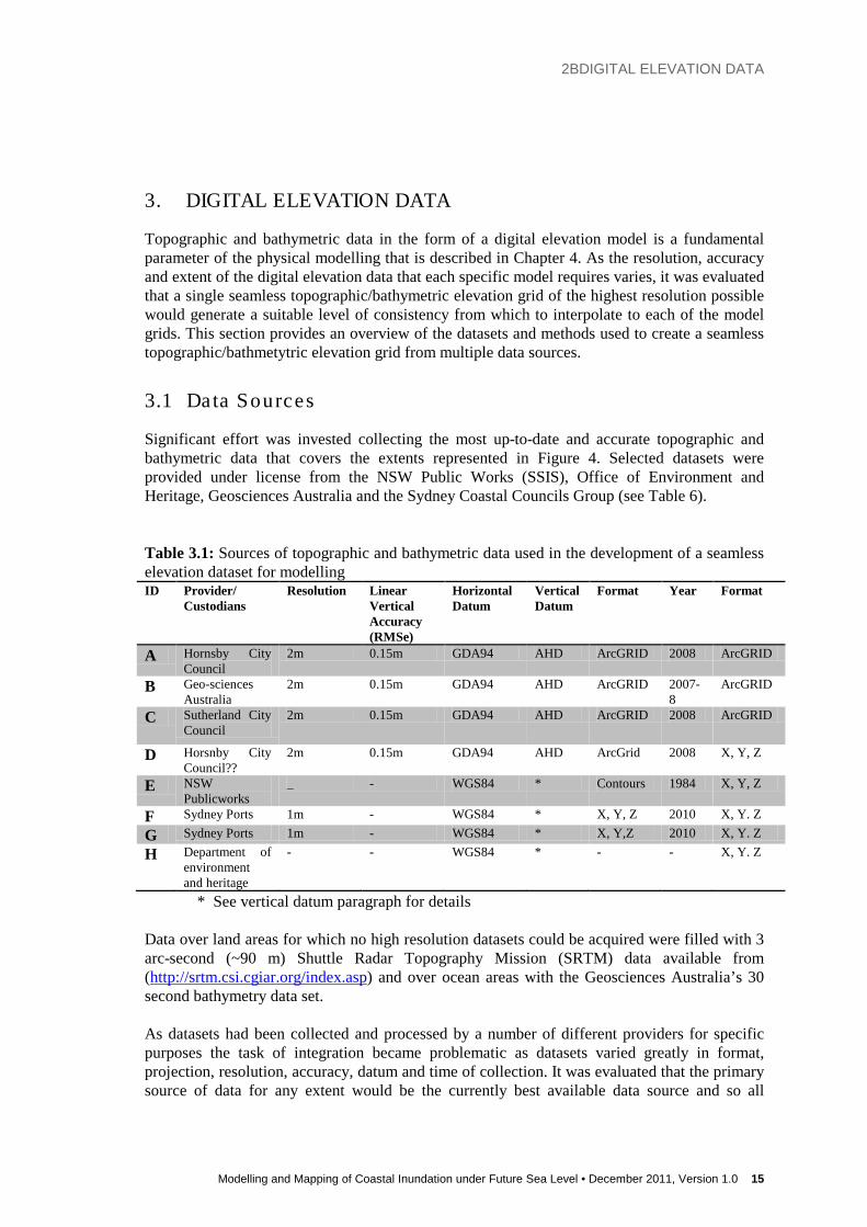
Significant effort was invested collecting the most up-to-date and accurate topographic and bathymetric data that covers the extents represented in Figure 4. Selected datasets were provided under license from the NSW Public Works (SSIS), Office of Environment and Heritage, Geosciences Australia and the Sydney Coastal Councils Group (see Table 6).
Table 3.1: Sources of topographic and bathymetric data used in the development of a seamless elevation dataset for modelling ID Provider/
Custodians Resolution Linear
Vertical Accuracy (RMSe)
Horizontal Datum
Vertical Datum
Format Year Format
A Hornsby City Council
2m 0.15m GDA94 AHD ArcGRID 2008 ArcGRID
B Geo-sciences Australia
2m 0.15m GDA94 AHD ArcGRID 2007-8
ArcGRID
C Sutherland City Council
2m 0.15m GDA94 AHD ArcGRID 2008 ArcGRID
D Horsnby City Council??
2m 0.15m GDA94 AHD ArcGrid 2008 X, Y, Z
E NSW Publicworks
_ - WGS84 * Contours 1984 X, Y, Z
F Sydney Ports 1m - WGS84 * X, Y, Z 2010 X, Y. Z
G Sydney Ports 1m - WGS84 * X, Y,Z 2010 X, Y. Z
H Department of environment and heritage
- - WGS84 * - - X, Y. Z
* See vertical datum paragraph for details Data over land areas for which no high resolution datasets could be acquired were filled with 3 arc-second (~90 m) Shuttle Radar Topography Mission (SRTM) data available from (http://srtm.csi.cgiar.org/index.asp) and over ocean areas with the Geosciences Australia’s 30 second bathymetry data set. As datasets had been collected and processed by a number of different providers for specific purposes the task of integration became problematic as datasets varied greatly in format, projection, resolution, accuracy, datum and time of collection. It was evaluated that the primary source of data for any extent would be the currently best available data source and so all
2BDIGITAL ELEVATION DATA
16 Modelling and Mapping of Coastal Inundation under Future Sea Level • December 2011, Version 1.0]
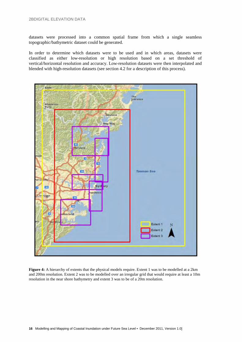
datasets were processed into a common spatial frame from which a single seamless topographic/bathymetric dataset could be generated. In order to determine which datasets were to be used and in which areas, datasets were classified as either low-resolution or high resolution based on a set threshold of vertical/horizontal resolution and accuracy. Low-resolution datasets were then interpolated and blended with high-resolution datasets (see section 4.2 for a description of this process).
Figure 4: A hierarchy of extents that the physical models require. Extent 1 was to be modelled at a 2km and 200m resolution. Extent 2 was to be modelled over an irregular grid that would require at least a 10m resolution in the near shore bathymetry and extent 3 was to be of a 20m resolution.

2BDIGITAL ELEVATION DATA
Modelling and Mapping of Coastal Inundation under Future Sea Level • December 2011, Version 1.0 17
Figure 3.2: The coverage of the acquired datasets. See table 6 for further details.
The common geospatial framework consisted of the following:
2BDIGITAL ELEVATION DATA
18 Modelling and Mapping of Coastal Inundation under Future Sea Level • December 2011, Version 1.0]
The common geospatial framework consisted of the following.
10m Grid Resolution As high-resolution grids can always be aggregated into lower resolution grids it was decided to interpolate the highest resolution possible for the extent of the case-study area.
GDA94 Horizontal datum This is the current standard datum in Australia (find references) and a common characteristic of most of the data provided. AHD Vertical datum Vertical datum is the most problematic integration parameter as bathymetric data/soundings normally set zero depth relative to the tide at the time of collection and the AHD is a datum that assigns zero based on the mean sea level between 1966-1968 at thirty tide gauges around the coast of the Australian continent. As AHD was adopted by the National Mapping Council as the datum to which all vertical control for mapping (and other surveying functions) all collected datasets referenced a conversion parameter that was used to determine elevation data in AHD.
Topographic LiDAR LiDAR data provided by the Sydney Coastal Councils included the Sutherland Sydney Council, Pittwater City Council and Hornsby City Council areas. Geo-sciences Australia provided the remaining part of the case-study area see Figure 5 and Table 6. LiDAR surveys were conducted by AAMHatch and were provided as gridded bare-earth tiles and .LAS files. The gridded bare earth tiles were used to generate the seamless topographic/bathymetric grid. The data was provided “as is” there was no attempt made to investigate possible flaws. LiDAR was received within the correct geospatial framework and date of acquisition were a year apart (2007-2008). The LiDAR data was aggregated into 10m grids for integration using the maximum cell value. Multibeam Bathymetry Multibeam bathymetric data is collected from a ship that detects the seafloor by resolving the returned echo into multiple beams. Multibeam data over Botany Bay and Sydney Harbour were provided by the Sydney Ports authority under a license agreement. No data was available over near shore areas that were to shallow for ships to travel over these areas were interpolated using the method described in section 3.2. 1984 Echo-Soundings Acquiring near shore bathymetry involved liaising with the NSW Public Works, they provided an extract from their SASIS (Surveying and Spatial Information Services) of all hydrological surveys conducted over the case study area. See appendix for reference. 20 maps of beach surveys conducted in 1984 using eco-sounding were completed. Though this data set was not ideal in terms of time of collection and vertical accuracy it was deemed suitable for the accuracy requirements of the hydro-dynamic modelling. Data was provided as PDF maps and a digitized version from the Office of Environment and Heritage. The data was provided “as is” and no no attempt made to investigate possible flaws in the data. Contour lines were provided in KML and were converted into ArcGIS Line format
2BDIGITAL ELEVATION DATA
Modelling and Mapping of Coastal Inundation under Future Sea Level • December 2011, Version 1.0 19
3.2 Development of Cons is tent Gridded Data
The merging of datasets classified as low-resolution was done using the ArcGIS 10 TOPOGRID which is an implementation of the ANUDEM thin spline interpolation algorithm which is optimized for the generation of topographic surfaces (Hutchinson ,1988, 1989). High resolution elevation points within 600 meters of low resolution dataset boundaries were included in the interpolation for the purpose of seamless merging of high-resolution data. In order to maintain the accuracy of the high resolution datasets the aggregated to 10m high resolution data was mosaicked onto the interpolated low-resolution grid with the 600m overlap between the datasets blended using a GIS function that performs weighted averaging on a cell-by-cell basis according to the proximity to the edges of the overlap area. The interpolation and merging process are a derivative of an approach described by (Gesch and Wilson 2002) for improving the best available regional elevation dataset by integrating the most up to date high-resolution local elevation data. Before settling on this approach a number of papers were reviewed for an appropriate elevation model creation that would “resample” or rather better represent the low resolution data on a 10m grid. A comparison of DEM creation methods is out of the scope of this paper but the following advantages of the ANUDEM interpolator were noted.
• Input elevation data can consist of ether point, line or polygon, the contour data could directly be utilized by the interpolator rather then having to convert them to elevation points.
• A file containing the parameters and datasets used in the ANU interpolator can easily be adjusted to include new high-resolution datasets as they become available and the grid creation procedure then becomes semi-automated.
• It has the most accessible scientific literature (Hutchinson 1988, Hutchinson 1989) and published criticisms (Greenberg, 2002). And case-studies from which a best use method could be determined.
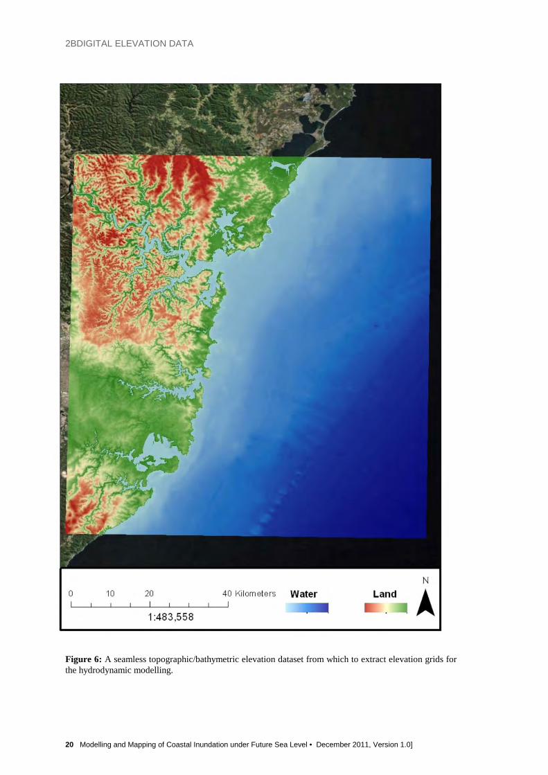
The spatial and vertical resolution of the output grid though coarse was sufficient enough to support the hydro-dynamic modelling at all three extents. The extent of the resultant topographic file is shown in Figure 6.
2BDIGITAL ELEVATION DATA
20 Modelling and Mapping of Coastal Inundation under Future Sea Level • December 2011, Version 1.0]
Figure 6: A seamless topographic/bathymetric elevation dataset from which to extract elevation grids for the hydrodynamic modelling.

3BHYDRODYNAMIC AND MODEL SETUP AND RESULTS
Modelling and Mapping of Coastal Inundation under Future Sea Level • December 2011, Version 1.0 21
4. HYDRODYNAMIC AND MODEL SETUP AND RESULTS
A suite of physical models were used in this study to dynamically model the sea levels arising from a storm surge and associated tides and wave setup. The linkages between the different models, and their geographical coverage is illustrated in Figure 7. The following sections describe the models and their implementation. Also, model results arising from the modelling of specific extreme sea level events identified in Section 2 are presented and discussed.
Figure 7: The hierarchy of models used in this study. Three horizontal spatial resolutions (2 km, 200m and 20m) were used for the hydrodynamic modelling using GCOM2D (coloured shading indicates the elevation across each model domain in m AHD). Atmospheric winds and pressure were interpolated to the spatial resolution of each model. The outermost 2km-resolution GCOM2D simulation included tidal forcing on its lateral boundaries. Modelled currents and sea levels due to wind, pressure and tidal forcing from the 2km simulation were applied to the lateral ocean boundaries of the 200m-resolution model. The 200m model provided simulated sea levels and currents to the SWAN wave model implemented on a variable resolution grid with significant wave heights and periods sourced from the Sydney wave-rider buoy applied along its lateral boundaries. A set of five 20m-resolution GCOM2D grids covering; 1-The Hawkesbury River, 2-Manly to Palm Beach, 3-Sydney Harbour, 4-Bondi Beach and 5-Botany Bay, obtained current and sea level boundary conditions from the 200m-resolution GCOM2D simulation and wave radiation stress forcing from the SWAN simulation to provide sea levels and currents due to tides, storm surge and wave setup.
3BHYDRODYNAMIC AND MODEL SETUP AND RESULTS
22 Modelling and Mapping of Coastal Inundation under Future Sea Level • December 2011, Version 1.0]
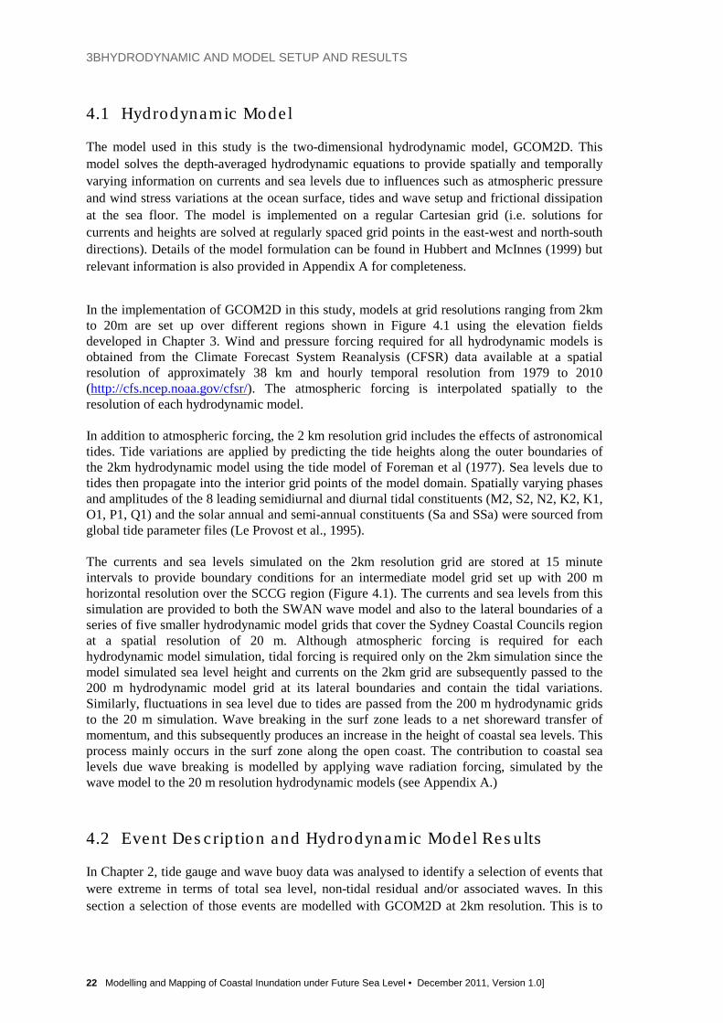
4.1 Hydrodynamic Model
The model used in this study is the two-dimensional hydrodynamic model, GCOM2D. This model solves the depth-averaged hydrodynamic equations to provide spatially and temporally varying information on currents and sea levels due to influences such as atmospheric pressure and wind stress variations at the ocean surface, tides and wave setup and frictional dissipation at the sea floor. The model is implemented on a regular Cartesian grid (i.e. solutions for currents and heights are solved at regularly spaced grid points in the east-west and north-south directions). Details of the model formulation can be found in Hubbert and McInnes (1999) but relevant information is also provided in Appendix A for completeness.
In the implementation of GCOM2D in this study, models at grid resolutions ranging from 2km to 20m are set up over different regions shown in Figure 4.1 using the elevation fields developed in Chapter 3. Wind and pressure forcing required for all hydrodynamic models is obtained from the Climate Forecast System Reanalysis (CFSR) data available at a spatial resolution of approximately 38 km and hourly temporal resolution from 1979 to 2010 (http://cfs.ncep.noaa.gov/cfsr/). The atmospheric forcing is interpolated spatially to the resolution of each hydrodynamic model. In addition to atmospheric forcing, the 2 km resolution grid includes the effects of astronomical tides. Tide variations are applied by predicting the tide heights along the outer boundaries of the 2km hydrodynamic model using the tide model of Foreman et al (1977). Sea levels due to tides then propagate into the interior grid points of the model domain. Spatially varying phases and amplitudes of the 8 leading semidiurnal and diurnal tidal constituents (M2, S2, N2, K2, K1, O1, P1, Q1) and the solar annual and semi-annual constituents (Sa and SSa) were sourced from global tide parameter files (Le Provost et al., 1995). The currents and sea levels simulated on the 2km resolution grid are stored at 15 minute intervals to provide boundary conditions for an intermediate model grid set up with 200 m horizontal resolution over the SCCG region (Figure 4.1). The currents and sea levels from this simulation are provided to both the SWAN wave model and also to the lateral boundaries of a series of five smaller hydrodynamic model grids that cover the Sydney Coastal Councils region at a spatial resolution of 20 m. Although atmospheric forcing is required for each hydrodynamic model simulation, tidal forcing is required only on the 2km simulation since the model simulated sea level height and currents on the 2km grid are subsequently passed to the 200 m hydrodynamic model grid at its lateral boundaries and contain the tidal variations. Similarly, fluctuations in sea level due to tides are passed from the 200 m hydrodynamic grids to the 20 m simulation. Wave breaking in the surf zone leads to a net shoreward transfer of momentum, and this subsequently produces an increase in the height of coastal sea levels. This process mainly occurs in the surf zone along the open coast. The contribution to coastal sea levels due wave breaking is modelled by applying wave radiation forcing, simulated by the wave model to the 20 m resolution hydrodynamic models (see Appendix A.)
4.2 Event Des crip tion and Hydrodynamic Model Res ults
In Chapter 2, tide gauge and wave buoy data was analysed to identify a selection of events that were extreme in terms of total sea level, non-tidal residual and/or associated waves. In this section a selection of those events are modelled with GCOM2D at 2km resolution. This is to
3BHYDRODYNAMIC AND MODEL SETUP AND RESULTS
Modelling and Mapping of Coastal Inundation under Future Sea Level • December 2011, Version 1.0 23
investigate firstly, how the model performs in representing the key processes that contribute to inundation from the combination of tides, storm surge and wave setup and secondly to identify a suitable event for the purposes of designing a storm to be used as a basis for the inundation modelling in Chapter 5. As discussed in section 2.1, extreme sea levels can arise from a range of processes. The suite of models used in this study represents the main drivers of short term, local extreme sea levels driven by a combination of severe weather and tides. Other contributions such as the remote influences from, for example CTW’s, seasonal or interannual variations in sea level from ENSO or transient eddy activity arising from the East Australian Current that lead to temporary sea level anomalies are not represented by the models used here. A criterion for selecting events caused by the combination of waves and storm surge, and not influenced by other processes is that they are well represented by GCOM2D. Therefore, the events and model results presented and discussed in this section will serve a dual purpose. They will identify events suitable for modelling in terms of severe weather forcing and they will also validate the model performance for an event that is suitable for inundation modelling.
4.2.1 Event 1: May 1997
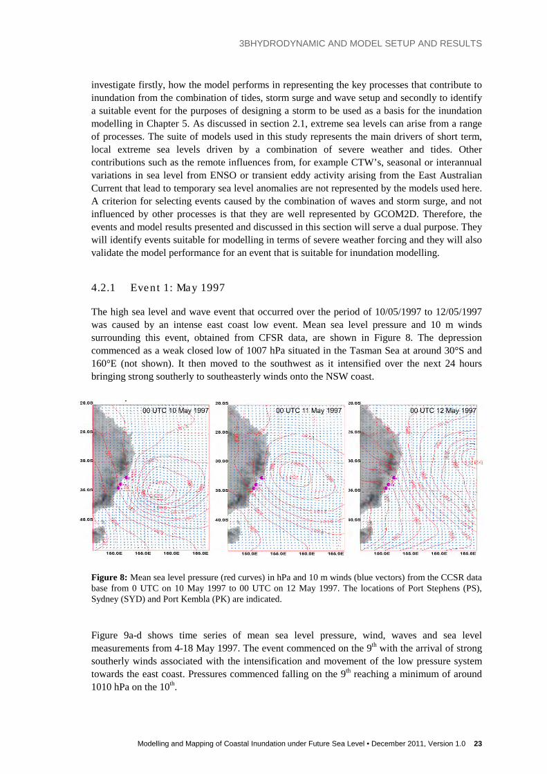
The high sea level and wave event that occurred over the period of 10/05/1997 to 12/05/1997 was caused by an intense east coast low event. Mean sea level pressure and 10 m winds surrounding this event, obtained from CFSR data, are shown in Figure 8. The depression commenced as a weak closed low of 1007 hPa situated in the Tasman Sea at around 30°S and 160°E (not shown). It then moved to the southwest as it intensified over the next 24 hours bringing strong southerly to southeasterly winds onto the NSW coast.
Figure 8: Mean sea level pressure (red curves) in hPa and 10 m winds (blue vectors) from the CCSR data base from 0 UTC on 10 May 1997 to 00 UTC on 12 May 1997. The locations of Port Stephens (PS), Sydney (SYD) and Port Kembla (PK) are indicated.
Figure 9a-d shows time series of mean sea level pressure, wind, waves and sea level measurements from 4-18 May 1997. The event commenced on the 9th with the arrival of strong southerly winds associated with the intensification and movement of the low pressure system towards the east coast. Pressures commenced falling on the 9th reaching a minimum of around 1010 hPa on the 10th.

3BHYDRODYNAMIC AND MODEL SETUP AND RESULTS
24 Modelling and Mapping of Coastal Inundation under Future Sea Level • December 2011, Version 1.0]
Figure 9: (a) Mean sea level pressure, and (b) observed wind speed and direction at Sydney Airport, wave direction, (b) observed significant wave height (Hs), wave period (Tsig), peak wave period (Tp1) and mean wave period (Tz) at the Sydney wave rider buoy and (c) total sea level (ζtot) , predicted tide (ζtid) and residual sea level (ζres = ζtot - ζtid) at the Fort Denison tide gauge over the period 4-18 May, 1997.

3BHYDRODYNAMIC AND MODEL SETUP AND RESULTS
Modelling and Mapping of Coastal Inundation under Future Sea Level • December 2011, Version 1.0 25
Wave direction shifted from easterly to southerly at the same time as the wind shift on the 9th (Figure 9b). Coinciding with the increase in wind speed at around 08 UTC 9 May, significant wave height (Hs) increased from 2 m to 6 m at 00 UTC 10 May to 8 m at 00 UTC 11 May. Significant wave period (Tsig) also increased from around 6 s to 12 s over this time, indicating the influence of more distant long period swell waves. The predicted tides indicate that the low pressure event commenced about a day after a spring tidal peak. Strong winds during this event led to an increase in coastal sea levels of over 0.3 m (Figure 9c). The atmospheric pressure during this event did not fall below 1010 hPa, which is around the average pressure for this latitude. Therefore the inverse barometer effect was not a major contributor to the elevated sea levels during this event. In fact, for much of this event, the higher pressures contributed to an increase in the height of residual sea levels of up to 0.1 m (9d).
Figure 10 compares the CFSR reanalysis data for Mean Sea Level Pressure (MSLP) and 10m winds with observations from Sydney Airport. MSLP shown in Figure 10a indicates that CFSR agrees well with observations. A comparison of the 10m wind speeds and directions indicates that the wind speeds from the CFSR underestimated those measured at Sydney airport (Figure 10b) while wind direction was well represented by the CFSR data throughout the event. The good agreement between observed and CFSR MSLP, wind direction and timing of wind speed increase suggests that the movement of the weather system was well captured. It was therefore considered reasonable to make an adjustment to the wind speed to bring the magnitudes into better alignment with the observations before application to the surge and wave models.
Figure 10: Mean sea level pressure, wind speed and direction for May 1997 observed at Sydney Airport (blue circles) and extracted from CFSR data at the same location (red curves).

3BHYDRODYNAMIC AND MODEL SETUP AND RESULTS
26 Modelling and Mapping of Coastal Inundation under Future Sea Level • December 2011, Version 1.0]
Two GCOM2D simulations were performed; one with tidal forcing only and one with tides and atmospheric forcing. Simulated values at Fort Denison and Port Kembla are compared with predicted tides for these locations provided by the National Tidal Centre (Paul Davill, pers. comm. 2010) and the observed sea levels at these gauges (Figure 11). Sea level heights from the tide-only simulation compare well with the predicted tides. In the simulation with atmospheric forcing additionally applied, simulated sea levels agree well with the measured sea levels. This is most apparent over the period from the 9-12 May when strong wind forcing leads to an elevation of sea levels above the tide-only levels.
Figure 11: Comparison of GCOM2D model simulations with tidal and meteorological forcing with observed sea levels and GCOM2D model simulations with tide only forcing with predicted tide heights at (a) Fort Denison and (b) Port Kembla for 6-15 May 1997.
4.2.2 Event 2: J une 1998
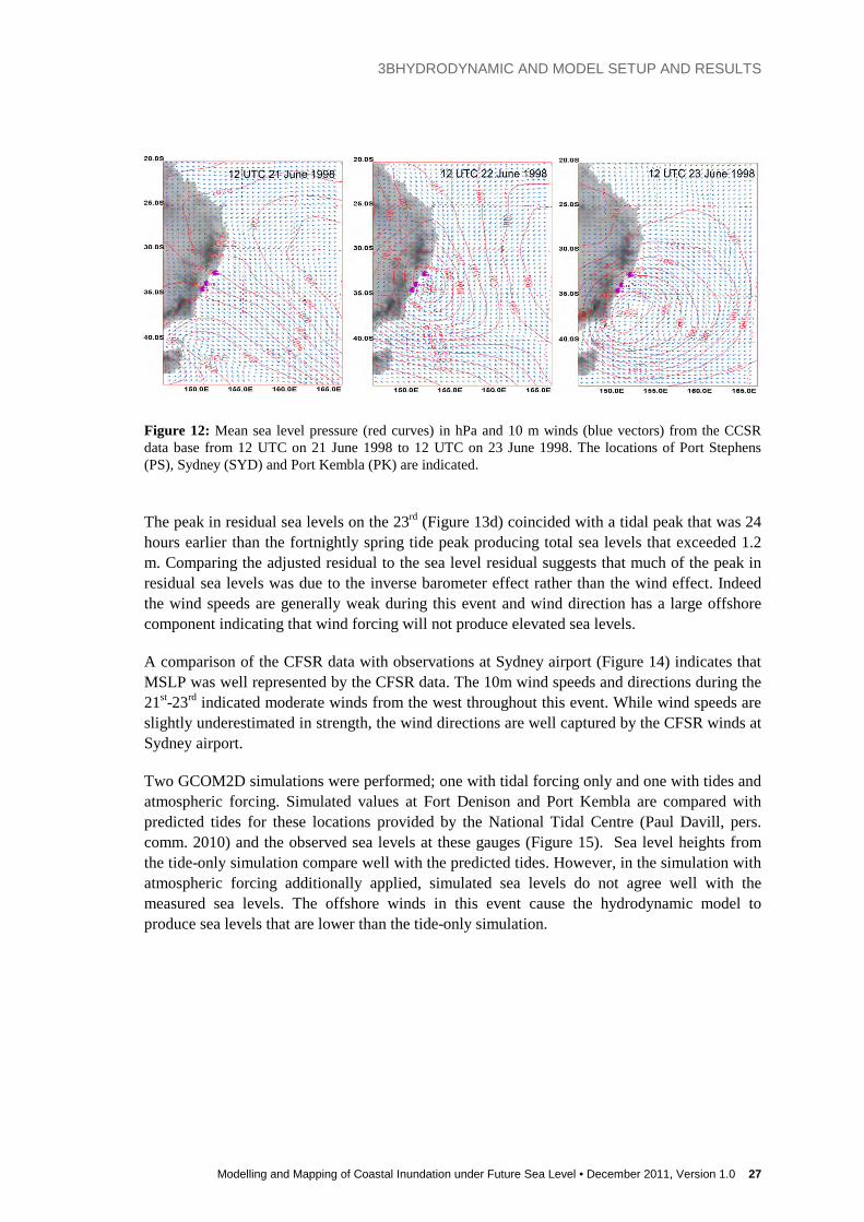
The high sea level and wave event that occurred over the period of 21/06/1998 to 23/06/1998 was caused by an intense low pressure system that developed over the southern NSW coast. Mean sea level pressure and 10 m winds surrounding this event and obtained from CFSR data are shown in Figure 12. A low pressure signature is evident at 40°S which had become a closed low with a minimum pressure of 1004 hPa near Sydney on the 22nd. The low intensified as it moved southwards along the coast during the next 24 hours, during which time gales and storm force winds were observed along the southern coast.
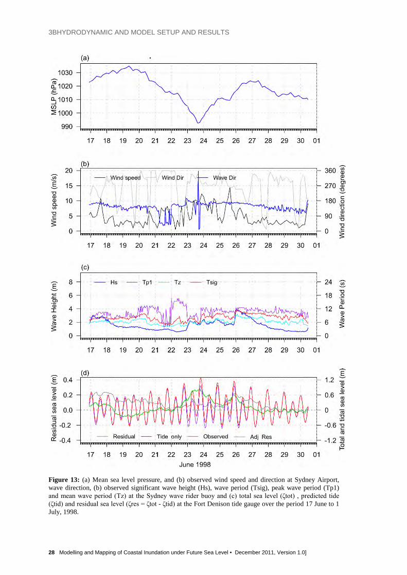
Figure 13a-d shows time series of mean sea level pressure, wind, waves and sea level measurements from 17-30 June 1998. Pressure commenced falling on the 20th and reached a minimum of around 993 hPa on the 23rd. Wave direction is mainly southerly throughout the event (Figure 13b). Significant wave height on the 22nd is around 1 m. Peak wave periods reach 15 s, indicating the influence of swell but shifts to shorter period peak waves of around 3 s on the 23rd. The predicted tides indicate that the event occurred close to a spring tide maximum.
3BHYDRODYNAMIC AND MODEL SETUP AND RESULTS
Modelling and Mapping of Coastal Inundation under Future Sea Level • December 2011, Version 1.0 27
Figure 12: Mean sea level pressure (red curves) in hPa and 10 m winds (blue vectors) from the CCSR data base from 12 UTC on 21 June 1998 to 12 UTC on 23 June 1998. The locations of Port Stephens (PS), Sydney (SYD) and Port Kembla (PK) are indicated.
The peak in residual sea levels on the 23rd (Figure 13d) coincided with a tidal peak that was 24 hours earlier than the fortnightly spring tide peak producing total sea levels that exceeded 1.2 m. Comparing the adjusted residual to the sea level residual suggests that much of the peak in residual sea levels was due to the inverse barometer effect rather than the wind effect. Indeed the wind speeds are generally weak during this event and wind direction has a large offshore component indicating that wind forcing will not produce elevated sea levels.
A comparison of the CFSR data with observations at Sydney airport (Figure 14) indicates that MSLP was well represented by the CFSR data. The 10m wind speeds and directions during the 21st-23rd indicated moderate winds from the west throughout this event. While wind speeds are slightly underestimated in strength, the wind directions are well captured by the CFSR winds at Sydney airport.
Two GCOM2D simulations were performed; one with tidal forcing only and one with tides and atmospheric forcing. Simulated values at Fort Denison and Port Kembla are compared with predicted tides for these locations provided by the National Tidal Centre (Paul Davill, pers. comm. 2010) and the observed sea levels at these gauges (Figure 15). Sea level heights from the tide-only simulation compare well with the predicted tides. However, in the simulation with atmospheric forcing additionally applied, simulated sea levels do not agree well with the measured sea levels. The offshore winds in this event cause the hydrodynamic model to produce sea levels that are lower than the tide-only simulation.
3BHYDRODYNAMIC AND MODEL SETUP AND RESULTS
28 Modelling and Mapping of Coastal Inundation under Future Sea Level • December 2011, Version 1.0]
Figure 13: (a) Mean sea level pressure, and (b) observed wind speed and direction at Sydney Airport, wave direction, (b) observed significant wave height (Hs), wave period (Tsig), peak wave period (Tp1) and mean wave period (Tz) at the Sydney wave rider buoy and (c) total sea level (ζtot) , predicted tide (ζtid) and residual sea level (ζres = ζtot - ζtid) at the Fort Denison tide gauge over the period 17 June to 1 July, 1998.

3BHYDRODYNAMIC AND MODEL SETUP AND RESULTS
Modelling and Mapping of Coastal Inundation under Future Sea Level • December 2011, Version 1.0 29
Figure 14: Mean sea level pressure, wind speed and direction for June 1998 observed at Sydney Airport (blue circles) and extracted from CFSR data at the same location (red curves).
Figure 15: Comparison of GCOM2D model simulations with tidal and meteorological forcing with observed sea levels and GCOM2D model simulations with tide only forcing with predicted tide heights at Fort Denison for 16-25 June 1998.

3BHYDRODYNAMIC AND MODEL SETUP AND RESULTS
30 Modelling and Mapping of Coastal Inundation under Future Sea Level • December 2011, Version 1.0]
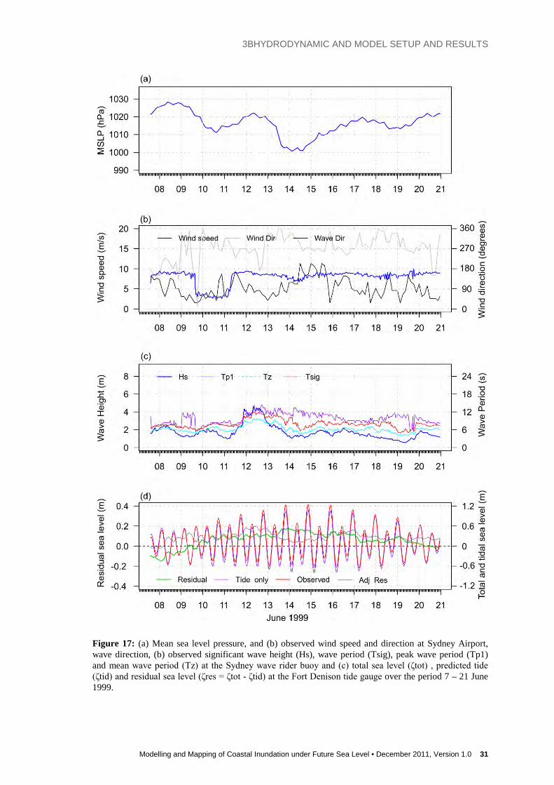
4.2.3 Event 3: J une 1999
The high sea level event that occurred over the period of 13/06/1999 to 15/06/1999 was associated with the passage of a cold front over southern NSW on the 13th. Over the next 2 days, southwesterly winds became established over the southern NSW becoming more westerly around Sydney and further north (Figure 16).
Figure 16: Mean sea level pressure (red curves) in hPa and 10 m winds (blue vectors) from the CCSR data base from 12 UTC on 13 June 1999 to 12 UTC on 15 June 1999. The locations of Port Stephens (PS), Sydney (SYD) and Port Kembla (PK) are indicated. Figure 17a-d shows time series of mean sea level pressure, wind, waves and sea level measurements from 8-21 June 1999. Pressure commenced falling on the 13th and reached a minimum of around 1001 hPa on the 14th. Wave direction is mainly southeasterly throughout the event (Figure 17b). Significant wave height peaks at just under 5 m on the 12th ahead of the fall in pressure on the 13th and 14th which coincides in a rise in residual sea levels of just under 0.2 m. A spring tidal peak occurs late on the 14th which is enhanced by the higher-than-normal sea level residuals. Comparing the adjusted residual to the sea level residual indicates that much of the peak in residual sea levels around the time of the peak in tidal levels on the 14th was due to the inverse barometer effect rather than the winds. The winds at Sydney are directed offshore which is not conducive for wind setup.
A comparison of the CFSR data with observations at Sydney airport indicate that surface pressure was well represented (Figure 18). The 10m wind speeds and directions during the 13th – 15th indicated moderate winds from the west throughout this event. While wind magnitudes are underestimated in strength, the wind directions are well captured by the CFSR winds at Sydney airport.
3BHYDRODYNAMIC AND MODEL SETUP AND RESULTS
Modelling and Mapping of Coastal Inundation under Future Sea Level • December 2011, Version 1.0 31
Figure 17: (a) Mean sea level pressure, and (b) observed wind speed and direction at Sydney Airport, wave direction, (b) observed significant wave height (Hs), wave period (Tsig), peak wave period (Tp1) and mean wave period (Tz) at the Sydney wave rider buoy and (c) total sea level (ζtot) , predicted tide (ζtid) and residual sea level (ζres = ζtot - ζtid) at the Fort Denison tide gauge over the period 7 – 21 June 1999.

3BHYDRODYNAMIC AND MODEL SETUP AND RESULTS
32 Modelling and Mapping of Coastal Inundation under Future Sea Level • December 2011, Version 1.0]
Figure 18: Mean sea level pressure, wind speed and direction for June 1999 observed at Sydney Airport (blue circles) and extracted from CFSR data at the same location (red curves). Two GCOM2D simulations were performed. The first had tidal forcing only and the second had tides and atmospheric forcing. Simulated values at Fort Denison are compared with predicted tides (provided by the National Tidal Centre by Paul Davill, pers. comm. 2010) and the observed sea levels at Fort Denison (Figure 19). Sea level heights from the tide-only simulation agree reasonably well with the predicted tides during the latter part of the simulation. However, similar to Event 2, the simulation with tide and atmospheric forcing produced sea levels that were again slightly lower than those in the tide-only simulation. Again, the offshore winds in this event are not conducive to producing elevated coastal sea levels. Measured sea levels are higher throughout the event period by about 0.3 m.
Figure 19: Comparison of GCOM2D model simulations with tidal and meteorological forcing with observed sea levels and GCOM2D model simulations with tide only forcing with predicted tide heights at Fort Denison for 7-16 June 1999.

3BHYDRODYNAMIC AND MODEL SETUP AND RESULTS
Modelling and Mapping of Coastal Inundation under Future Sea Level • December 2011, Version 1.0 33
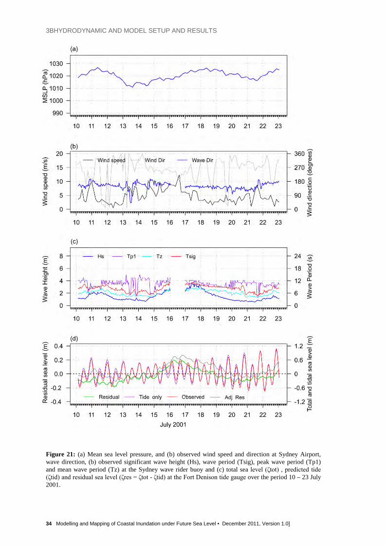
4.2.4 Event 4: J u ly 2001
The high sea level event that occurred over the period of 27-29 July 2001 was caused by an inland low pressure trough which deepened as it moved off the NSW coast (Figure 20). Strong southerly winds reached gale force at times generating waves and swell of 4 to 6 m.
Figure 20: Mean sea level pressure (red curves) in hPa and 10 m winds (blue vectors) from the CCSR data base from 00 UTC on 27 July 2001 to 00 UTC on 29 July 2001. The locations of Port Stephens (PS), Sydney (SYD) and Port Kembla (PK) are indicated.
Figure 21a-d shows time series of mean sea level pressure, wind, waves and sea level measurements from 8-21 June 1999. Pressure commenced falling on the 13th and reached a minimum of around 1001 hPa on the 14rd. Wave direction is mainly southeasterly throughout the event (Figure 21b). Significant wave height peaks at just under 5 m on the 12th ahead of the fall in pressure on the 13th and 14th which coincides in a rise in residual sea levels of just under 0.2 m. A spring tidal peak occurs late on the 14th which is enhanced by the higher than normal sea level residuals. Comparing the adjusted residual to the sea level residual indicates that much of the peak in residual sea levels around the time of the peak in tidal levels on the 14th was due to the inverse barometer effect rather than the winds. The winds at Sydney are directed offshore which is not conducive for wind setup
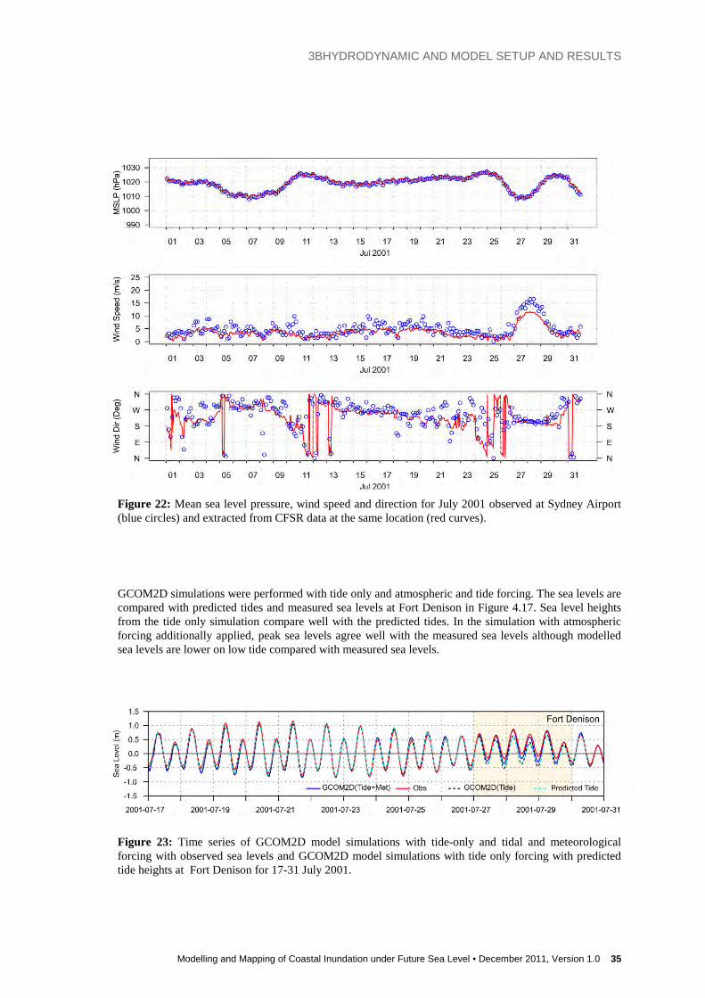
Figure 22 compares the CFSR reanalysis data for Mean Sea Level Pressure (MSLP) and 10m winds with observations from Sydney Airport. MSLP shown in Figure 22a indicates that CFSR agrees well with observations. A comparison of the 10m wind speeds and directions indicates that the wind speeds from the CFSR underestimated those measured at Sydney airport (Figure 22b) while wind direction was well represented by the CFSR data throughout the event (Figure 22c). An adjustment to the wind speed was therefore made to bring the magnitudes into better alignment with the observations before application to the surge and wave models.
3BHYDRODYNAMIC AND MODEL SETUP AND RESULTS
34 Modelling and Mapping of Coastal Inundation under Future Sea Level • December 2011, Version 1.0]
Figure 21: (a) Mean sea level pressure, and (b) observed wind speed and direction at Sydney Airport, wave direction, (b) observed significant wave height (Hs), wave period (Tsig), peak wave period (Tp1) and mean wave period (Tz) at the Sydney wave rider buoy and (c) total sea level (ζtot) , predicted tide (ζtid) and residual sea level (ζres = ζtot - ζtid) at the Fort Denison tide gauge over the period 10 – 23 July 2001.
3BHYDRODYNAMIC AND MODEL SETUP AND RESULTS
Modelling and Mapping of Coastal Inundation under Future Sea Level • December 2011, Version 1.0 35
Figure 22: Mean sea level pressure, wind speed and direction for July 2001 observed at Sydney Airport (blue circles) and extracted from CFSR data at the same location (red curves).
GCOM2D simulations were performed with tide only and atmospheric and tide forcing. The sea levels are compared with predicted tides and measured sea levels at Fort Denison in Figure 4.17. Sea level heights from the tide only simulation compare well with the predicted tides. In the simulation with atmospheric forcing additionally applied, peak sea levels agree well with the measured sea levels although modelled sea levels are lower on low tide compared with measured sea levels. Figure 23: Time series of GCOM2D model simulations with tide-only and tidal and meteorological forcing with observed sea levels and GCOM2D model simulations with tide only forcing with predicted tide heights at Fort Denison for 17-31 July 2001.
3BHYDRODYNAMIC AND MODEL SETUP AND RESULTS
36 Modelling and Mapping of Coastal Inundation under Future Sea Level • December 2011, Version 1.0]
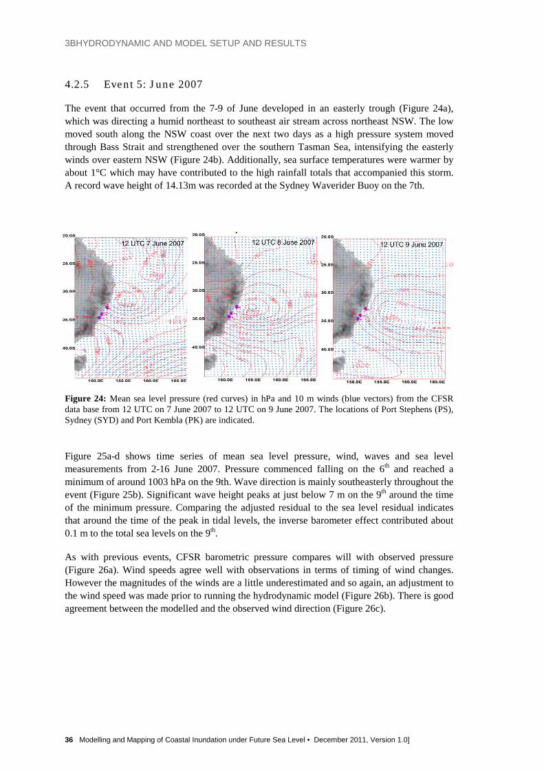
4.2.5 Event 5: J une 2007
The event that occurred from the 7-9 of June developed in an easterly trough (Figure 24a), which was directing a humid northeast to southeast air stream across northeast NSW. The low moved south along the NSW coast over the next two days as a high pressure system moved through Bass Strait and strengthened over the southern Tasman Sea, intensifying the easterly winds over eastern NSW (Figure 24b). Additionally, sea surface temperatures were warmer by about 1°C which may have contributed to the high rainfall totals that accompanied this storm. A record wave height of 14.13m was recorded at the Sydney Waverider Buoy on the 7th.
Figure 24: Mean sea level pressure (red curves) in hPa and 10 m winds (blue vectors) from the CFSR data base from 12 UTC on 7 June 2007 to 12 UTC on 9 June 2007. The locations of Port Stephens (PS), Sydney (SYD) and Port Kembla (PK) are indicated.
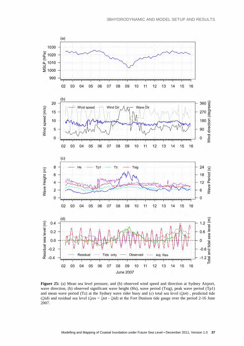
Figure 25a-d shows time series of mean sea level pressure, wind, waves and sea level measurements from 2-16 June 2007. Pressure commenced falling on the 6th and reached a minimum of around 1003 hPa on the 9th. Wave direction is mainly southeasterly throughout the event (Figure 25b). Significant wave height peaks at just below 7 m on the 9th around the time of the minimum pressure. Comparing the adjusted residual to the sea level residual indicates that around the time of the peak in tidal levels, the inverse barometer effect contributed about 0.1 m to the total sea levels on the 9th.
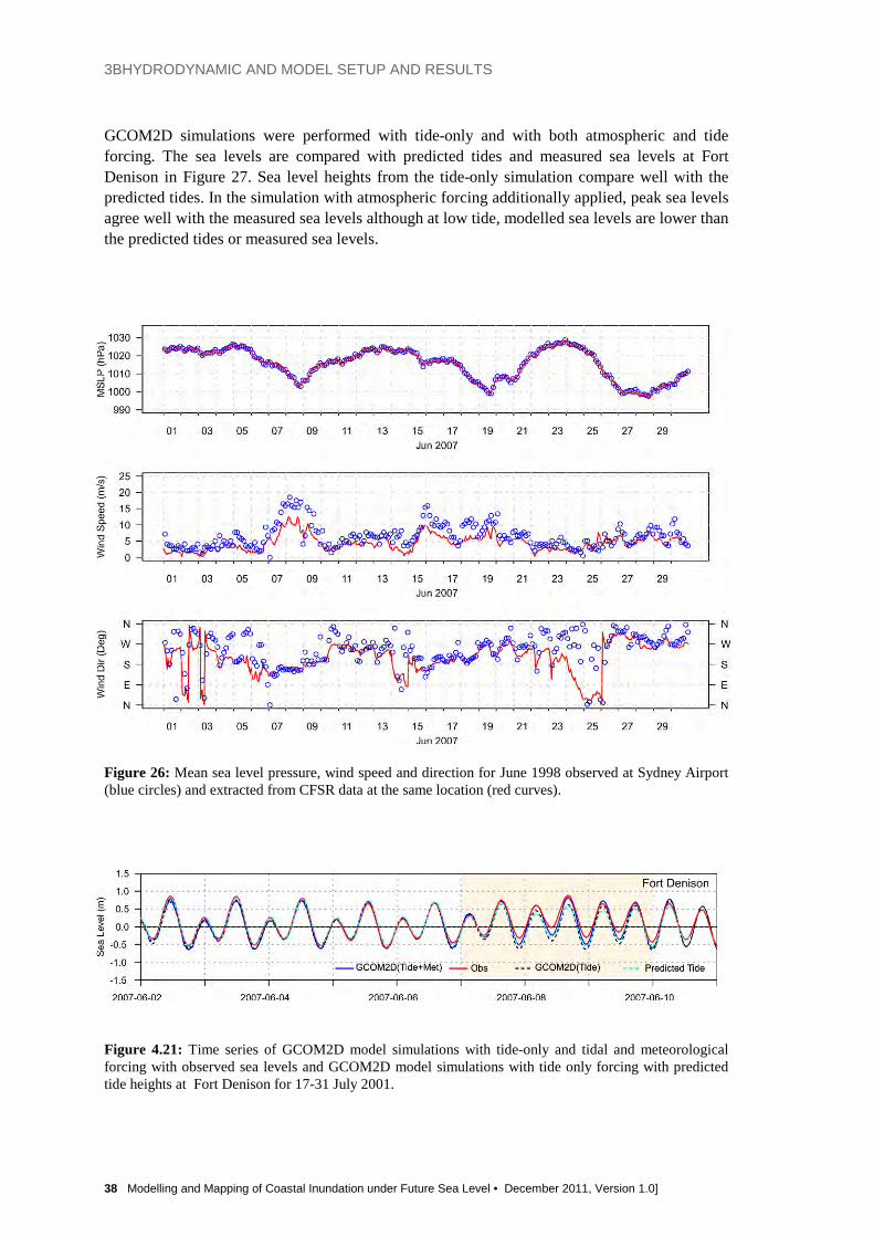
As with previous events, CFSR barometric pressure compares will with observed pressure (Figure 26a). Wind speeds agree well with observations in terms of timing of wind changes. However the magnitudes of the winds are a little underestimated and so again, an adjustment to the wind speed was made prior to running the hydrodynamic model (Figure 26b). There is good agreement between the modelled and the observed wind direction (Figure 26c).
3BHYDRODYNAMIC AND MODEL SETUP AND RESULTS
Modelling and Mapping of Coastal Inundation under Future Sea Level • December 2011, Version 1.0 37
Figure 25: (a) Mean sea level pressure, and (b) observed wind speed and direction at Sydney Airport, wave direction, (b) observed significant wave height (Hs), wave period (Tsig), peak wave period (Tp1) and mean wave period (Tz) at the Sydney wave rider buoy and (c) total sea level (ζtot) , predicted tide (ζtid) and residual sea level (ζres = ζtot - ζtid) at the Fort Denison tide gauge over the period 2-16 June 2007.
3BHYDRODYNAMIC AND MODEL SETUP AND RESULTS
38 Modelling and Mapping of Coastal Inundation under Future Sea Level • December 2011, Version 1.0]
GCOM2D simulations were performed with tide-only and with both atmospheric and tide forcing. The sea levels are compared with predicted tides and measured sea levels at Fort Denison in Figure 27. Sea level heights from the tide-only simulation compare well with the predicted tides. In the simulation with atmospheric forcing additionally applied, peak sea levels agree well with the measured sea levels although at low tide, modelled sea levels are lower than the predicted tides or measured sea levels.
Figure 26: Mean sea level pressure, wind speed and direction for June 1998 observed at Sydney Airport (blue circles) and extracted from CFSR data at the same location (red curves). Figure 4.21: Time series of GCOM2D model simulations with tide-only and tidal and meteorological forcing with observed sea levels and GCOM2D model simulations with tide only forcing with predicted tide heights at Fort Denison for 17-31 July 2001.
3BHYDRODYNAMIC AND MODEL SETUP AND RESULTS
Modelling and Mapping of Coastal Inundation under Future Sea Level • December 2011, Version 1.0 39
4.3 Wave Model Implementa tion
The Simulating WAves Nearshore (SWAN) model is used in this study to model the wave field and the nearshore radiation stress terms (BOOIJ et al, 1999). SWAN is a spectral wave model and is classed as a third generation wave model because it represents non-linear wave-wave interactions. SWAN is formulated in terms of the spectral action balance equation (energy density divided by the relative wave frequency). Action density (rather than energy density) is used because this quantity is conserved in the presence of currents, making SWAN particularly suitable for shallow, near coastal applications where coastal currents may be significant. The model also represents the modification of wave energy through processes such as wave energy growth through winds, and dissipation through whitecapping, bottom friction and depth-induced wave breaking and energy transfer due to wave interaction. The SWAN model has been formulated on an unstructured grid over the region shown in Figure 4.1 so that spatial resolution in the coastal zone is maximised. The specification of the triangular grid was achieved using the triangle program available at http://www-2.cs.cmu.edu/~quake/triangle.html. In the specification of the grid, the individual triangles were constrained to have angles no less than 28° and areas no greater than 0.001 nautical degrees squared following the method of constrained Delaunay triangulation (Shewchuk, 2002). Elevation data, discussed in Chapter 3, was interpolated to the wave model grid. The coastal boundary was defined to be at the 2.5 m elevation contour. This was to allow for maximum sea level perturbations due to tides as well as allow for landward adjustment of the coastline that occurs with the application of mean sea level rise scenarios. Wind forcing for the model was obtained from CFSR winds and sea level heights and currents were obtained from the 200 m resolution GCOM2D simulation. Observational wave buoy data from the Sydney directional wave buoy located at 33.78°S 151.42°E was used to specify wave characteristics on the southern and eastern boundaries of the wave model. A spectrum of wave heights based on empirical observational data (i.e. JONSWAP spectrum) is specified within the models for specified observational values of Hs, Tp and Wd. Although observations of waves are not available at the coast for wave model validation, we examine how the model responds to the inclusion of the effects of winds, varying surge and tide levels and currents over the nearshore region. Two simulations were performed. The first run (the ‘waves-only’ run), had wave parameters from the observations at the Sydney wave rider buoy applied to its ocean boundaries. The second simulation had, in addition to the wave forcing, wind forcing from the CFSR winds and currents and sea levels simulated by GCOM2D imposed and is referred to as the ‘all effects’ run. Figure 28 compares the difference between the ‘all-effects’ and ‘waves-only’ simulations at high tide (Figure 28a) and low tide (Figure 28b). These anomaly patterns show that the effect of the wind forcing is most apparent in the northern half of the model domain centred on 151.4°E with the higher wave heights of up to 0.3 m being attained in the ‘all-effects’ run. This is due to the greater fetch from the southeasterly winds during this event. Differences in the spatial pattern of the anomalies between the low and high tide examples are because the time difference between the two figures is 5 hours, over which time the relative wind and wave forcing has evolved. In the shallow water immediately adjacent to the coast, the effect of the differences in background sea level due to the tidal variations can be seen. At low tide, wave heights in the ‘all effects’ simulation are lower than the ‘waves-only’ simulation whereas at high tide, wave heights in the ‘all-effects’ simulation are higher than the ‘waves-only’ simulation. This is because at low tide, the effect of bottom friction is felt further offshore resulting in wave steepening, breaking and energy dissipation and a reduction of wave heights commencing further offshore and so that lower wave heights result at a fixed geographical point close to the shore at low tide compared to zero tide.

3BHYDRODYNAMIC AND MODEL SETUP AND RESULTS
40 Modelling and Mapping of Coastal Inundation under Future Sea Level • December 2011, Version 1.0]
Conversely, at high tide, waves steepen and break closer into shore so that less energy and wave height reduction occurs compared to the zero tide case. An examination of the time varying differences in wave height arising from the variation in tide levels is shown in Figure 29 for two points indicated by (a) and (b) in Figure 28. The water depth at both points is approximately 5 m. The simulation with ‘waves and wind’ is similar to the ‘waves-only’ simulation. However, when ‘water level’ information due to tides and surge is included in the simulations, wave heights reduce by about 0.2 m at low tide and increase by around the same amount at high tide relative to the ‘wave-only’ and ‘waves and wind’ simulations. The addition of current data does not have a discernibly different response from the ‘waves, wind and water level’ simulation. Figure 28: Differences in wave height calculated from the ‘all effects’ simulation minus the ‘waves only’ SWAN simulation at (a) low tide and (b) high tide. Figure 29: Differences in wave height calculated from the ‘all effects’ simulation minus the ‘waves only’ SWAN simulation at (a) low tide and (b) high tide.

3BHYDRODYNAMIC AND MODEL SETUP AND RESULTS
Modelling and Mapping of Coastal Inundation under Future Sea Level • December 2011, Version 1.0 41
4.4 Des ign S torm Cons truc tion and Sea Level Scenarios
For the purposes of modelling inundation, it was considered that sea levels corresponding to a 1-in-1 year and a 1-in-100 year event at Fort Denison were the most appropriate levels to base the modelling on. Of the 5 events in Table 5 that were modelled in Section 4.2, Events 1, 4 and 5 validated well against measured sea levels for both ‘tide-only’ and ‘tide and meteorology’ simulations where as Events 2 and 3 validated well only for the ‘tide-only’ simulation. Since Event 1 produced a peak sea level at Fort Denison that was close to a 1-in-1 year event, it was therefore selected to form the basis of the design storm construction for the inundation modelling. To increase the peak sea level attained by this event to 1.24 m AHD, the level assessed by Watson and Lord (2008) to be a 1 in 1 year event (Table 1), wind speeds were increased by 3% in the hydrodynamic modelling. To obtain sea levels consistent with a 1-in-100 year event of 1.45 m AHD, the atmospheric conditions from Event 1 were phased with the spring tides that occurred in Event 2, so that a 1.45 m AHD sea level was attained at Fort Denison. The time series of the two events are shown in Figure 30.
Figure 30: Time series showing the sea levels at Fort Denison arising from the 1-in-1 year and 1 in 100 year design storms over 24 hours of the simulation. The sea level peaks occur at different times of the day because of the phasing of the storm forcing with tide forcing at a different time of the tidal cycle in each event.
The NSW Government Coastline Management Manual. ISBN 0730575063. (available at http://www.environment.gov.au/archive/coasts/publications/nswmanual/index.html recommends that sea level rise planning benchmarks for use in assessing the potential impacts of projected sea level rise in coastal areas should consider 0.4 metres by 2050 and 0.9 metres by 2100 relative to a 1980-1999 reference period. Allowing for the different reference periods between the sea level rise estimates and the return levels reported in Table 1, Table 7 lists the relevant extreme sea level values at Fort Denison to be considered in the extreme sea level modelling. The sea level rise allowance was accounted in the models by subtracting the value of the sea level rise from the elevation data used by the wave and hydrodynamic models at all grid resolutions. This changes the mean sea level value used by the model. Table 7: Fort Denison water levels combined with sea level rise scenarios for 2050 and 2100.
Return Period (yrs)
Fort Denison water levels combinedSea Level Rise Scenario 2010 2050 2100
1 1.24 1.58 2.08 100 1.44 1.78 2.28
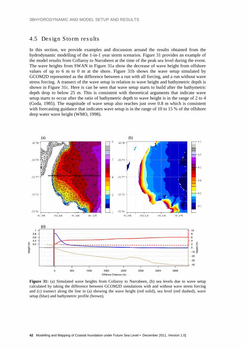
3BHYDRODYNAMIC AND MODEL SETUP AND RESULTS
42 Modelling and Mapping of Coastal Inundation under Future Sea Level • December 2011, Version 1.0]
4.5 Des ign S torm res ults
In this section, we provide examples and discussion around the results obtained from the hydrodynamic modelling of the 1-in-1 year storm scenarios. Figure 31 provides an example of the model results from Collaroy to Narrabeen at the time of the peak sea level during the event. The wave heights from SWAN in Figure 31a show the decrease of wave height from offshore values of up to 6 m to 0 m at the shore. Figure 31b shows the wave setup simulated by GCOM2D represented as the difference between a run with all forcing, and a run without wave stress forcing. A transect of the wave setup in relation to wave height and bathymetric depth is shown in Figure 31c. Here is can be seen that wave setup starts to build after the bathymetric depth drop to below 25 m. This is consistent with theoretical arguments that indicate wave setup starts to occur after the ratio of bathymetric depth to wave height is in the range of 2 to 4 (Goda, 1985). The magnitude of wave setup also reaches just over 0.8 m which is consistent with forecasting guidance that indicates wave setup is in the range of 10 to 15 % of the offshore deep water wave height (WMO, 1998).
Taking the
Figure 31: (a) Simulated wave heights from Collaroy to Narrabeen, (b) sea levels due to wave setup calculated by taking the difference between GCOM2D simulations with and without wave stress forcing and (c) transect along the line in (a) showing the wave height (red solid), sea level (red dashed), wave setup (blue) and bathymetric profile (brown).
(a) (b)
(c)
(a) (b)
(c)

3BHYDRODYNAMIC AND MODEL SETUP AND RESULTS
Modelling and Mapping of Coastal Inundation under Future Sea Level • December 2011, Version 1.0 43
A second example from Cronulla is shown in Figure 32. Again, the simulated wave setup values and profile are similar to those of Figure 31. It is also worth noting that values are not uniform along the coast. For example at the northeastern end of the beach, the presence of a reef leads to wave breaking and higher values of wave setup on the seaward side of the reef. Wave heights on the ocean side of the reef are around 5 m whereas behind the reef, wave breaking has lowered the wave heights to around 2.5 to 3 m.
Figure 32: (a) Simulated wave heights over Collaroy, (b) sea levels due to wave setup calculated by taking the difference between GCOM2D simulations with and without wave stress forcing and (c) transect along the line in (a) showing the wave height (red solid), sea level (red dashed), wave setup (blue) and bathymetric profile (brown).
(a)
(b)
(c)
Merri’sReef
(a)
(b)
(c)
(a)
(b)
(c)
(a)
(b)
(c)
Merri’sReef
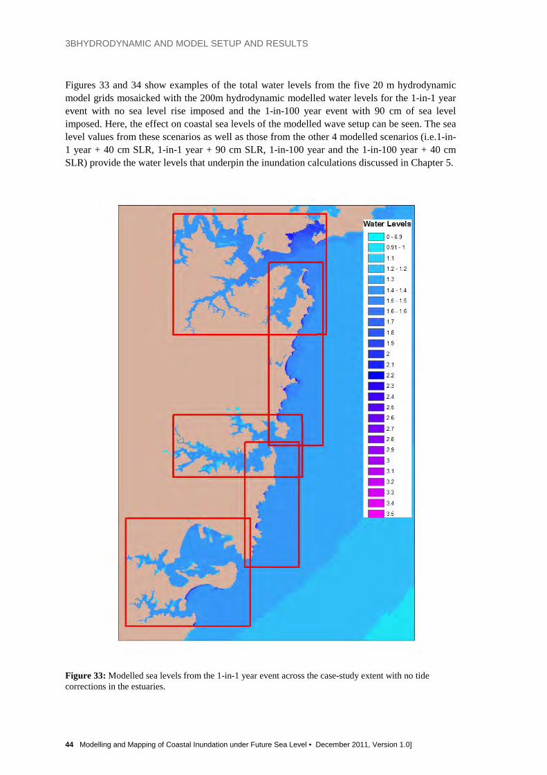
3BHYDRODYNAMIC AND MODEL SETUP AND RESULTS
44 Modelling and Mapping of Coastal Inundation under Future Sea Level • December 2011, Version 1.0]
Figures 33 and 34 show examples of the total water levels from the five 20 m hydrodynamic model grids mosaicked with the 200m hydrodynamic modelled water levels for the 1-in-1 year event with no sea level rise imposed and the 1-in-100 year event with 90 cm of sea level imposed. Here, the effect on coastal sea levels of the modelled wave setup can be seen. The sea level values from these scenarios as well as those from the other 4 modelled scenarios (i.e.1-in-1 year + 40 cm SLR, 1-in-1 year + 90 cm SLR, 1-in-100 year and the 1-in-100 year + 40 cm SLR) provide the water levels that underpin the inundation calculations discussed in Chapter 5.
Figure 33: Modelled sea levels from the 1-in-1 year event across the case-study extent with no tide corrections in the estuaries.

3BHYDRODYNAMIC AND MODEL SETUP AND RESULTS
Modelling and Mapping of Coastal Inundation under Future Sea Level • December 2011, Version 1.0 45
Figure 34: Modelled sea levels from the 1-in-100 year event under a 90 cm sea level rise across the case-study extent with no tide corrections in the estuaries.
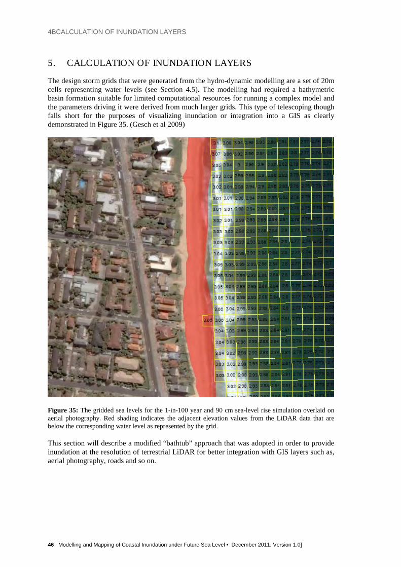
4BCALCULATION OF INUNDATION LAYERS
46 Modelling and Mapping of Coastal Inundation under Future Sea Level • December 2011, Version 1.0]
5. CALCULATION OF INUNDATION LAYERS
The design storm grids that were generated from the hydro-dynamic modelling are a set of 20m cells representing water levels (see Section 4.5). The modelling had required a bathymetric basin formation suitable for limited computational resources for running a complex model and the parameters driving it were derived from much larger grids. This type of telescoping though falls short for the purposes of visualizing inundation or integration into a GIS as clearly demonstrated in Figure 35. (Gesch et al 2009)
Figure 35: The gridded sea levels for the 1-in-100 year and 90 cm sea-level rise simulation overlaid on aerial photography. Red shading indicates the adjacent elevation values from the LiDAR data that are below the corresponding water level as represented by the grid. This section will describe a modified “bathtub” approach that was adopted in order to provide inundation at the resolution of terrestrial LiDAR for better integration with GIS layers such as, aerial photography, roads and so on.
4BCALCULATION OF INUNDATION LAYERS
Modelling and Mapping of Coastal Inundation under Future Sea Level • December 2011, Version 1.0 47
5.1 Rationa le
The use of low resolution grids when mapping inundation yields only a broad representation of vulnerable land (Dean, 2009) as vertical accuracy is lost during preprocessing techniques like\ interpolation or aggregation. Recent studies have demonstrated that the significantly higher accuracy and resolution of LiDAR derived elevation grids provide clear advantages for identifying and delineating lands subject to a sea-level rise scenario (Gesch 2009a). These studies utilize the “bathtub” method which relies on a comparison of the maximum total water height to ground elevation. If an elevation grid point is lower than the maximum total water height it is assumed to be flooded. The accuracy of the approach is dependent upon the accuracy and resolution of the elevation grid (Gesch, 2009a) yet is able to process the highest quality elevation grid available with significantly less computational overheads. Yet the “bathtub” method is traditionally not a dynamic model and makes the assumption that a water level modelled at the coast will infill terrain at lower elevation to the same level. The average point spacing of the LiDAR data provided by the Sydney Coastal Council (illustrated in Chapter 3) is estimated to be 1.4m and the vertical accuracy is estimated to be 0.15m at a 68% confidence level using the ArcGIS natural neighbour irregular grid interpolator. This dataset is clearly of the highest quality and most suitable for identifying land vulnerable to inundation. In summary the bathtub approach can utilize the advantages of a high resolution dataset and is flexible enough in its method of assigning water levels for it to be informed by the hydrodynamic modelling output grids over the coast line, enabling the creation of inundation layers suitable for integration with high accuracy GIS layers.
5.2 Methodology
A method was devised as part of this study in which LiDAR derived elevation points within the range of maximum water heights (4m) were extracted and converted to GIS points. A shore line and estuary delineation in the form of 57,000 lines representing all water bodies connected to the coast over the case-study area were extracted from the hydrology layer of the PSMA Transport and Topography dataset (http://www.psma.com.au/products/transportandtopography.html). A water level is assigned to each line segment of the shore-line and estuary delineation by determining the closest water table grid point for each event. Then all LiDAR derived elevation points closest to the shore line are queried on whether they are lower than the water level value at the shore line. If they are then they are classified as inundated. See Figure 36 for an example. The assumption is that if a hydraulic flow path exists between a point and a shoreline all points that fall below the maximum water height calculated by the hydrodynamic model are assumed to be inundated. The approach currently does not consider hydraulic factors such as connectivity, storage and resistance.

4BCALCULATION OF INUNDATION LAYERS
48 Modelling and Mapping of Coastal Inundation under Future Sea Level • December 2011, Version 1.0]
Figure 36: The 1-in-100 year storm and 90 cm sea-level rise water level data overlaid on top of aerial photography red line marks out PSMA delineated shoreline boundary and yellow points are terrestrial LiDAR below 4m. Water Heights are assigned to the shoreline by querying the closest 20m cell for a water level per design storm. To portray the uncertainty in potential inundation levels calculated from elevation data, the absolute vertical accuracy of the data must be known at a 95% confidence (Gesch and etc). L.E. at 95% confidence = 1.96 * RMSE = 0.30m Two layers are extracted per event- an inundation layer and an inundation including the maximum vertical error in the LiDAR. Adjustments to the water levels were made along water bodies by applying a gradient that is calculated by the amount of linear change over an estuaries meandering distance. These adjustments were made using the relative values between tide heights that are given in Table
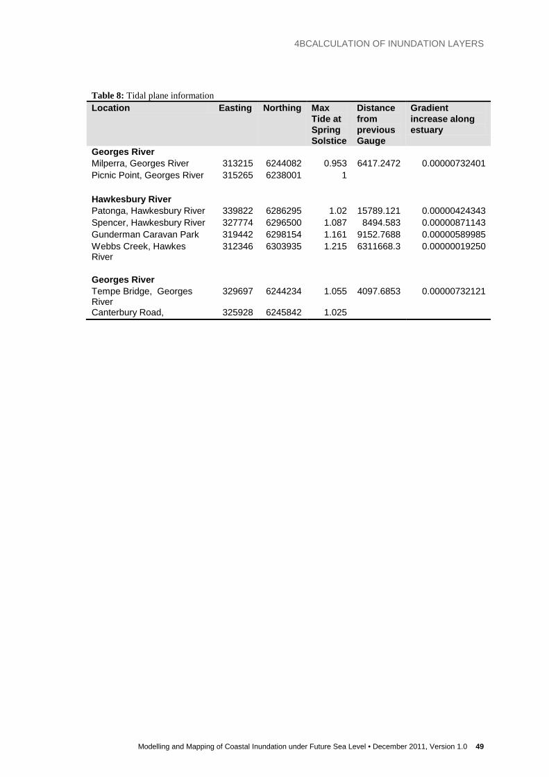
4BCALCULATION OF INUNDATION LAYERS
Modelling and Mapping of Coastal Inundation under Future Sea Level • December 2011, Version 1.0 49
Table 8: Tidal plane information Location Easting Northing Max
Tide at Spring Solstice
Distance from previous Gauge
Gradient increase along estuary
Georges River Milperra, Georges River 313215 6244082 0.953 6417.2472 0.00000732401 Picnic Point, Georges River 315265 6238001 1 Hawkesbury River Patonga, Hawkesbury River 339822 6286295 1.02 15789.121 0.00000424343 Spencer, Hawkesbury River 327774 6296500 1.087 8494.583 0.00000871143 Gunderman Caravan Park 319442 6298154 1.161 9152.7688 0.00000589985 Webbs Creek, Hawkes River
312346 6303935 1.215 6311668.3 0.00000019250
Georges River Tempe Bridge, Georges River
329697 6244234 1.055 4097.6853 0.00000732121
Canterbury Road, 325928 6245842 1.025

5BDISCUSSION AND CONCLUSION
50 Modelling and Mapping of Coastal Inundation under Future Sea Level • December 2011, Version 1.0]
6. DISCUSSION AND CONCLUSION
The Sydney Coastal Councils region spans around 100 km of coastline from Botany Bay in the south to the Hawkesbury River in the north and includes a complex coastal region consisting of open beaches, lagoons and estuarine environments. Over this extensive and diverse coastal region, a range of hydrodynamic drivers contribute to extreme coastal sea levels and inundation. Storm surges from severe weather events combine with tides to elevate sea levels across the region. However, on coastal beaches, wave breaking processes further enhance sea levels so that the maximum sea level achieved during an extreme event will vary considerably at different points along the coastline as a function of a range of coastal attributes such as the bathymetric depth profile, exposure to prevailing winds and waves, and so on.
The challenge in this study therefore, was to bring together the necessary modelling tools, techniques and data to develop a consistent approach for estimating the extreme sea levels that contribute to inundation across the entire Sydney Coastal Councils region. It was also necessary to develop a method for calculating and mapping inundation at a scale that is appropriate and relevant for the end users of this information. Finally, an important consideration was to develop a framework that would allow the work developed in this study to be built upon as and when required. During the course of this study, the merits of the different approaches and end-user needs were assessed and a methodology was devised that uses a combination of physical modelling to capture the different physical processes responsible for extreme sea levels together with high resolution mapping to deliver detailed information on coastal vulnerability to inundation.
A key requirement for this project was high quality and high resolution terrestrial elevation data. However, the importance of wave processes along the open coasts required that high resolution bathymetric data was also necessary to underpin the wave and hydrodynamic modelling. A major accomplishment in this project has been the sourcing of relevant elevation data, which has then been combined into a single seamless dataset appropriate for the hydrodynamic, wave modelling and inundation mapping components of this study.
The second challenge was around the capturing of the key physical processes that contribute to elevated sea levels and inundation. While tides and storm surge provide the largest contribution to the still water level throughout much of the SCC region, wave breaking contributions are also extremely important on the ocean beaches. Wave breaking processes contribute to potential inundation in two ways; through wave setup and wave runup. Wave setup increases the elevation of the still water level during a storm event through the cumulative effect of breaking of waves and can be modelled with a hydrodynamic model if the necessary wave stress fields can be simulated. Wave runup is a transitory contribution to inundation, which is also important because it can lead to water reaching several metres higher than the level attained by the combination of tide, storm surge and wave setup. However the inclusion of wave runup was beyond the scope and resources of the current project. Therefore in this study, the physical response of the ocean was simulated by coupling a hydrodynamic model with a coastal wave model. The hydrodynamic model captured the variations in sea level due to the associated weather system and tides sea levels of the selected events. Validation of the

5BDISCUSSION AND CONCLUSION
Modelling and Mapping of Coastal Inundation under Future Sea Level • December 2011, Version 1.0 51
nearshore wave modelling was not possible since relevant data was not available for validation. However, the wave and hydrodynamic models were shown to produce physically realistic representations of the coastal sea levels. The coupling of these physical models to provide a dynamically consistent representation of the variations in coastal sea levels is another major accomplishment of this project.
The SCC region covers an extensive length of coastline and in order to simulate the processes at the highest possible resolution, it was necessary to cut the SCCG into a series of 5 small subregions with a model resolution of 20 m. A dynamic wetting and drying algorithm in the hydrodynamic model physically modelled the overland inundation over the 5 subregions. However, it was found that in places, the dynamically modelled areas of inundation did not match well with areas of potentially vulnerable land based on the high resolution (2 m) LiDAR. This was due to the loss of accuracy that occurred in averaging elevation data to specify elevation at 20 m resolution for the hydrodynamic model grids. It was therefore decided that a more suitable method for creating elevation layers was to take the modelled sea levels at the position of the coastline and use a ‘bathtub’ fill approach to generate overland inundation using the terrestrial LiDAR at its native resolution.
The approach devised in this study to combine the physical modelling with GIS mapping has other benefits as well. For example, the approach lends itself to the inclusion of other types of data that may be considered in the future. For example, the calculation of wave runup, which is typically achieved through the use of empirical relationships along coastal transects, could be readily incorporated through this approach. Although the inclusion of wave runup was beyond the scope of the current project, the approach that has been developed in this study means that it would be possible to consider additional affects of this contribution in the future.

REFERENCES
52 Modelling and Mapping of Coastal Inundation under Future Sea Level • December 2011, Version 1.0]
REFERENCES
Booij, N., R.C. Ris and L.H. Holthuijsen, 1999, A third-generation wave model for coastal
regions, Part I, Model description and validation, J.Geoph.Research, 104, C4, 7649-7666
Bruun, P. (1988). The Bruun Rule of erosion by sea level rise. Journal of Coastal Research, 4, 627-648.
Church, J. A. and N.J. White (2011), Sea-level rise from the late 19th to the early 21st Century. Surveys in Geophysics, 32, 585-602, doi:10.1007/s10712-011-9119-1
Church, J.A., J.M. Gregory, N.J. White, S.M. Platten, and J.X. Mitrovica. 2011. Understanding and projecting sea level change. Oceanography 24(2):130–143, http://dx.doi.org/10.5670/oceanog.2011.33.
Department of Climate Change, 2009: Climate Change Risks to Australia’s Coast. A First Pass National Assessment. Report published by the Australian Government’s Department of Climate Change, 172 pp. http://www.climatechange.gov.au/publications (15/07/10)
Department of Environment Climate Change and Water. (1990). NSW Coastline Management Manual. Sydney: NSW Government.
Department of Environment Climate Change and Water. (2007). Floodplain Risk Management Guide - Practical Consideration of Climate Change. Sydney: Department of Environment Climate Change and Water NSW.
Department of Environment Climate Change and Water. (2010a). Coastal Risk Management Guide: Incorporating sea level rise benchmarks in coastal risk assessments. Sydney: Department of Environment Climate Change and Water NSW.
Department of Environment Climate Change and Water. (2010b). Flood Risk Management Guide - incorporating sea level rise benchmarks in flood risk assessments Sydney: Department of Environment Climate Change and Water NSW.
Department of Infrastructure Planning and Natural Resources. (2005). Floodplain Development Manual NSW. Sydney: Department of Infrastructure, Planning and Natural Resources.
Department of Planning. (2005). Sydney Harbour Foreshores and Waterways Area Development Control Plan). Sydney.
Foreman GG (1977) Manual for tidal heights analysis and prediction, Pacific Marine Science Report 77-10. Institute of Ocean Sciences, Victoria, Canada, 98 pp
Gesch, D.B., (2009) Analysis of Lidar elevation data for improved identification and delineation of lands vulnerable to sea level rise: Journal of Coastal Research, v. 53, no. SI, p. 49-58. (Also available online at http://topotools.cr.usgs.gov/pdfs/jcr_gesch_SI53.pdf.)
Gesch, D.B., (2009), Mapping and visualization of storm-surge dynamics for Hurricane Katrina and Hurricane Rita: U.S. Geological Survey Scientific Investigations Report, 2009-5230, 19 p. (Also available online at http://pubs.er.usgs.gov/publication/sir20095230.)
Gesch, D.B., and Wilson, R., (2002) Development of a seamless multisource topographic/bathymetric elevation model of Tampa Bay: Marine Technology Society Journal, v. 35, no. 4, p. 58-64. (Also available online at http://dx.doi.org/10.4031/002533201788058062.)
Goda, Y. (1985). Random Seas and Design of Maritime Structures. University of Tokyo Press, Japan, 325 pp.
Greenberg, H., (2001) Making Topogrid look bad: problems inherent in grid-based topographic analysis, http://duff.geology.washington.edu/mdbrg/mdbrg/topotest/
REFERENCES
Modelling and Mapping of Coastal Inundation under Future Sea Level • December 2011, Version 1.0 53
Harley M.D., I.L. Turner, A.D. Short and R. Ranasinghe (2010) Interannual variability and controls of the Sydney wave climate. International Journal of Climatology. DOI: 10.1002/joc.1962
Hubbert, G. D., and McInnes, K. L. (1999). A storm surge inundation model for coastal planning and impact studies. Journal of Coastal Research, 15 (1): 168-185.
Hutchinson, M. F. (1988) Calculation of hydrologically sound digital elevation models. Paper presented at Third International Symposium on Spatial Data Handling at Sydney, Australia.
Hutchinson, M. F. (1989) A new procedure for gridding elevation and stream line data with automatic removal of spurious pits. Journal of Hydrology, 106: 211–232.
IPCC (2007) Climate Change 2007: The Physical Science Basis. Contribution of Working Group I to the Fourth Assessment Report of the Intergovernmental Panel on Climate Change. Cambridge, University Press, Cambridge, UK and New York, USA, 996 pp
Manly Hydraulics Laboratory (MHL, 1992). Mid New South Wales Coastal Region, Tide-Storm Surge Analysis. Technical Report No: MHL621.
Manly Hydraulics Laboratory (MHL, 1997). New South Wales Coast May 1997 Storm Analysis. Technical Report No: MHL886, December.
Manly Hydraulics Laboratory (MHL, 2008). NSW Estuary and River Water Levels Annual Summary 2007-2008. Technical Report No: MHL1847, October 2008.
Manly Hydraulics Laboratory (MHL, 2011). NSW Ocean Water Levels. Technical Report No: MHL1881, March. 347pp.
McInnes KL, O’Grady JG, Hemer M, Macadam I, Abbs DJ, White CJ, Bennett JC, Corney SP, Holz GK, Grose MR, Gaynor SM & Bindoff NL 2011, Climate Futures for Tasmania: extreme tide and sea-level events technical report, Antarctic Climate and Ecosystems Cooperative Research Centre, Hobart, Tasmania.
McInnes, K. L., Abbs, D. A., O'Farrell, S. P., Macadam, I., O'Grady, J., & Ranasinghe, R. (2007). Projected Changes in Climatological Forcing for Coastal Erosion in NSW. CSIRO Marine and Atmospheric Research, Hobart: a project undertaken for the Department of Environment and Climate Change NSW.
McInnes, K. L., O'Grady, J., & Hubbert, G. D. (2009). Modelling Sea Level Extremes from Storm Surges and Wave Setup for Climate Change Assessments in Southeastern Australia. Journal of Coastal Research, Special Issue 56, 1005-1009.
McInnes, K. L., Hubbert, G. D., (2003). A Numerical modelling study of storm surges in Bass Strait. Australian Meteorological Magazine. Volume 52, No. 3. September 2003.
McInnes, K.L. and Hubbert, G.D. (2001) The impact of eastern Australian cut-off lows on coastal sea levels. Meteorological Applications, 8, 229-243.
McInnes, K.L., Abbs, D., O'Farrell, S., Macadam, I., O'Grady, J., Ranasinghe, R., (2007) Projected changes in climatological forcing for coastal erosion in NSW. NSW Department of Environment and Climate Change, 38 pp.
McInnes, K.L., I. Macadam, G.D. Hubbert and J.G. O'Grady (2009), A Modelling Approach for Estimating the Frequency of Sea Level Extremes and the Impact of Climate Change in Southeast Australia. Natural Hazards, 51, 115-137, doi:10.1007/s11069-009-9383-2.
McInnes, K.L., Macadam, I., Hubbert, G.D. and O’Grady, J.G. (2011). An assessment of current and future vulnerability to coastal inundation due to sea level extremes in Victoria, southeast Australia (submitted to Int. J. Clim.).
Menendez, M., and P.L. Woodworth, 2010: Changes in extreme high water levels based on a quasi-global tide-gauge dataset. Journal of Geophysical Research, 115(C10011)
Mount R, Lacey M, and Hunter J, (2010). Tasmanian Coastal Inundation Mapping Project. Report for Tasmanian Planning Commission.
NSW Government (1990). Coastline Management Manual. ISBN 0730575063. (available at http://www.environment.gov.au/archive/coasts/publications/nswmanual/index.html

REFERENCES
54 Modelling and Mapping of Coastal Inundation under Future Sea Level • December 2011, Version 1.0]
Ranasinghe, R., R. McLoughlin, A. Short and G. Symonds (2004), The Southern Oscillation Index, wave climate, and beach rotation. Marine Geology, 204, 273-287.
Shand, T.D., Mole, M.A., Carley, J.T., Peirson, W.L. and Cox, R.J. (2011) Coastal storm data analysis: Provision of Extreme Wave Data for Adaptation Planning. Water Research Laboratory Research Report 242. 145pp.
Shewchuk, J.R. (2002) Delaunay Refinement Algorithms for Triangular Mesh Generation, Computational Geometry: Theory and Applications 22(1-3):21-74.
Watson P.J and D.B. Lord (2008). “Fort Denison Sea Level Rise Vulnerability Study”. A report prepared by the Coastal Unit, Department of Environment and Climate Change, October 2008.
WMO (1988). Guide to wave analysis and forecasting. World Meteorological Organization, Report No. 702.
Woodworth PL, Mene´ndez M, Gehrels WR (2011) Evidence for century-timescale acceleration in mean sea levels and for recent changes in extreme sea levels. Surv Geophys 32, this issue. doi:10.1007/s10712-011-9112-8
Woodworth, P. L. and D. L. Blackman (2004). "Evidence for systematic changes in extreme high waters since the mid-1970's." Journal of Climate, 17(6): 1190-1197.

APPENDIX A
Modelling and Mapping of Coastal Inundation under Future Sea Level • December 2011, Version 1.0 55
APPENDIX A
The model used in this study is the two-dimensional hydrodynamic model, GCOM2D. This model solves the depth-averaged hydrodynamic equations to provide spatially and temporally varying information on currents and sea levels due to influences such as atmospheric pressure and wind variations, tides and wave setup on a regular Cartesian grid. The shallow water equations solved by this model are given in equations (1)-(3).
∂∂
+∂∂
−∂∂
−∂∂
−=∂∂
yUV
xUUm
xPm
xmgfV
tU
ωρζ ,1 2U
dyS
xS
Hxyxx
bxsx ∇−
∂−
∂∂
−−+ νττρω
(1)
∂∂
+∂∂
−∂∂
−∂∂
−−=∂∂
yVV
xVUm
yPm
ymgfU
tV
ωρζ ,1 2V
y
S
x
S
Hyyyx
bysy ∇−
∂
∂−
∂
∂−−+ νττ
ρω (2)
.2
∂∂
+
∂∂
−=∂∂
mVH
ymUH
xm
tζ (3)
Here U and V are the depth averaged currents in the x and y coordinate directions respectively, H is the total depth, ζ is the surface elevation, f is the Coriolis parameter, g is the acceleration due to gravity, m is the map factor (a scaling which depends on the chosen map projection of the model grid), P is the atmospheric surface pressure, ρw is the water density, ν is the coefficient of lateral eddy diffusion and has a value of 0.2, τsx,τyx,τbx and τby, the surface wind and bed frictional stresses in the x and y directions, respectively.
The bed stress terms are specified following the formulation of Signell and Butman (1992) according to;
( ) ( )22
2/1
222
2/1
2
; VUVH
gnVUUH
gnwbywbx +
+=+
+=
ςρτ
ςρτ (4)
where n has the value 0.0264.
The wind stress terms are specified from the 10 m wind speed using the formulation of Smith and Banke
2222 ; aaawDsyaaawDsx vuvCvuuC +=+= ρτρτ (5)
where ua and va are the x and y components of wind speed respectively, 22aaa vuu += ,
and CD=(0.63+0.066 au )×10-3 when au <20 ms-1 and CD=(0.63+0.033( au -20.0 )×10-3 when
au >20 ms-1.
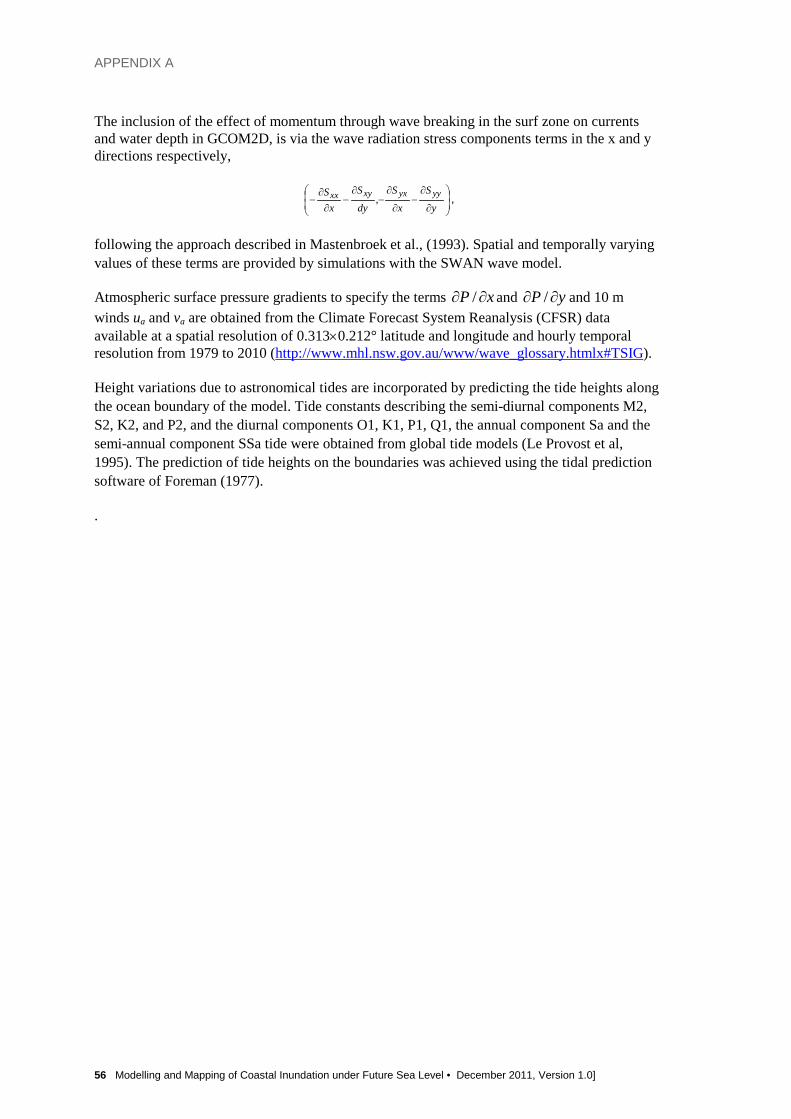
APPENDIX A
56 Modelling and Mapping of Coastal Inundation under Future Sea Level • December 2011, Version 1.0]
The inclusion of the effect of momentum through wave breaking in the surf zone on currents and water depth in GCOM2D, is via the wave radiation stress components terms in the x and y directions respectively,
∂
∂−
∂
∂−
∂−
∂∂
−y
S
x
S
dy
S
xS yyyxxyxx , ,
following the approach described in Mastenbroek et al., (1993). Spatial and temporally varying values of these terms are provided by simulations with the SWAN wave model.
Atmospheric surface pressure gradients to specify the terms xP ∂∂ / and yP ∂∂ / and 10 m winds ua and va are obtained from the Climate Forecast System Reanalysis (CFSR) data available at a spatial resolution of 0.313×0.212° latitude and longitude and hourly temporal resolution from 1979 to 2010 (http://www.mhl.nsw.gov.au/www/wave_glossary.htmlx#TSIG).
Height variations due to astronomical tides are incorporated by predicting the tide heights along the ocean boundary of the model. Tide constants describing the semi-diurnal components M2, S2, K2, and P2, and the diurnal components O1, K1, P1, Q1, the annual component Sa and the semi-annual component SSa tide were obtained from global tide models (Le Provost et al, 1995). The prediction of tide heights on the boundaries was achieved using the tidal prediction software of Foreman (1977).
.


This page can be removed if you are using pre-printed report covers. If you are not using pre-printed covers this page is to remain for all electronic and other printing types. Specific contact details are to be included at the front of this report above the Distribution list, Copyright and Disclaimers.