Barometr regionalny

tom 13 nr 4

Modelling and Forecasting Cash Withdrawals in the Bank

Jarosław Bielak, Andrzej BurdaUniversity of Management and Administration in Zamość, Poland

Mieczysław KowerskiUniversity of Information Technology and Management in Rzeszów, Poland

Krzysztof PancerzUniversity of Rzeszów, Poland

AbstractThe goal of the paper is searching for the optimal forecasting model estimating the amount of cash wi-thdrawn daily by the customers of one of the Polish banks by means of statistical and machine learning methods. The methodology of model creation and assessment criteria are significantly different for the models considered in the paper — i.e., for ARMAX and MLP. However, the comparison of forecasts ge-nerated by both models seems to be useful. Variables and attributes reflecting the calendar effects, used in both models, in case of obtained errors of forecasts less than 20%, showed a significant, non-linear influence of this type of predictors on the amount of the daily cash withdrawals at the bank, and hence on the amount of the daily declared cash limit.

Keywords: bank cash withdrawals forecasts, ARMAX and MLP models

Introduction

Determining the amount of money the bank has every day to ensure undisturbed cash withdrawals for its customers is an important and difficult issue . Exceeding the daily customers’ demands for cash is the cost of the bank — i .e ., the loss of benefits resulting from the inability to invest cash in other profitable ventures in that time . This cost is typically measured by the interest rate of inter-bank transactions . On the other hand, the lack of cash, even temporary, is the cost of the loss of customers’ confidence in the bank, difficult to measure, leading to a serious threat . A quick trans-port from the Central Bank can be the answer to the lack of cash . However, it is associated with the additional cost of transport .

Some banks typically maintain as much as 40% more cash than it is needed, even though many experts consider cash excess of 15% to 20% to be sufficient (Simutis, Dilijonas, and Bas-tina 2008, 416) . Through cash management optimization, banks can avoid falling into the trap of maintaining too much or too little cash . Therefore, it is very important to apply proper forecasting methods of cash demand . Each bank, in order to ensure the continuity of the customers’ service, must determine the level of the daily limit of cash, understood as the minimal level of cash, in the bank, ensuring the continuity of the customers’ service . This limit should be based on estimation of cash flows in the bank . The part of this market is determined and realized on the basis of con-tracts between banks . However, for the majority of banks, a significant part of their cash turnover is the customers’ deposits and withdrawals . Their forecasting can be affected by a big mistake . Determining the amount of cash flows can be estimated on the basis of the knowledge of the past customers’ behavior — i .e ., by means of inductive reasoning .

© 2015 by Wyższa Szkoła Zarządzania i Administracji w ZamościuAll Rights Reserved

166 Jarosław Bielak, Andrzej Burda, Mieczysław Kowerski, Krzysztof Pancerz

This problem is not new . It has a wide range of research and developments around the world as well as in Poland . It is a problem of better understanding of customers’ habits . Already, the first empirical studies in the 1980s made it possible, among others, to note that customers’ demands for cash show sensibility to calendar effects . 1 The calendar effects are an important feature of econom-ic data, given that most economic time series are directly or indirectly linked, to a daily activity which is usually recorded on a daily, monthly, quarterly or some other periodicity . Thus, the daily value of cash withdrawals may be influenced by daily calendar effects . The number of working days and its relation with seasonal effects are noticeable examples . Apart from the number of working days, the day of the week, the week of the month and other calendar effects such as public holidays or religious events 2 may also affect time series . Calendar effects are typically masked by strong seasonal patterns, because they are generally second-order effects only observed after other sources of variation have been accounted for (Esteves and Rodrigues 2010, 2–3) . There are also important salary and pension paydays as well as locations of cash dispensers . Recently in Poland, the wide research on this issue was conducted by Gurgul and Suder (Gurgul and Suder 2013a, 2013b, 2015) .

The goal of our research is searching for the optimal model estimating the amount of cash withdrawn daily by the customers of one of the Polish banks by means of statistical and machine learning methods .

1 Methodology

In the literature, techniques used for cash demand forecasting can be broadly classified into four groups (Darwish 2013, 405–406):

•time series methods that predict future cash need based on the past values of variable and/or past errors

•a factor analysis method, which is based on the determination of various factors that influence the cash demand pattern and calculating their correlation with actual cash withdrawals; in this group, the econometric models can be included

•a fuzzy expert system approach that tries to imitate the reasoning of a human operator; the idea is to reduce the analogical thinking behind the intuitive forecasting to formal steps of logic

•a neural networks approach that maps the relationships between various factors affecting the cash withdrawals and the actual cash withdrawals

In our research, we used methods of time series analysis and econometric modeling as well as ar-tificial neural networks belonging to machine learning methods .

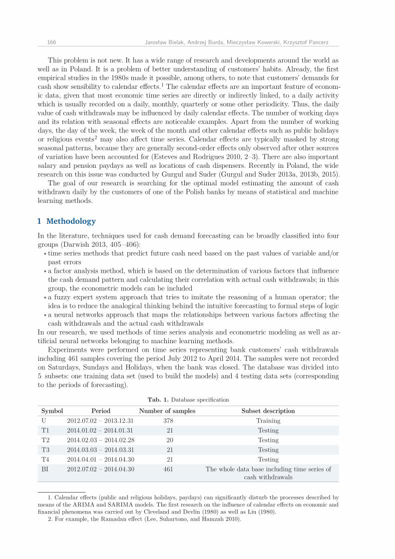
Experiments were performed on time series representing bank customers’ cash withdrawals including 461 samples covering the period July 2012 to April 2014 . The samples were not recorded on Saturdays, Sundays and Holidays, when the bank was closed . The database was divided into 5 subsets: one training data set (used to build the models) and 4 testing data sets (corresponding to the periods of forecasting) .

1. Calendar effects (public and religious holidays, paydays) can significantly disturb the processes described by means of the ARIMA and SARIMA models. The first research on the influence of calendar effects on economic and financial phenomena was carried out by Cleveland and Devlin (1980) as well as Liu (1980).

2. For example, the Ramadan effect (Lee, Suhartono, and Hamzah 2010).

Tab. 1. Database specification

Symbol Period Number of samples Subset descriptionU 2012 .07 .02 – 2013 .12 .31 378 TrainingT1 2014 .01 .02 – 2014 .01 .31 21 TestingT2 2014 .02 .03 – 2014 .02 .28 20 TestingT3 2014 .03 .03 – 2014 .03 .31 21 TestingT4 2014 .04 .01 – 2014 .04 .30 21 TestingBI 2012 .07 .02 – 2014 .04 .30 461 The whole data base including time series of

cash withdrawals

Modelling and Forecasting Cash Withdrawals in the Bank 167

As predicted (dependent) variables, we used daily withdrawals in PLN (Y) as well as the natu-ral logarithm of daily withdrawals (lnY) . 3

Our analysis of withdrawal distributions in the considered periods enabled us to distinguish the following predictors (independent variables), identified as descriptive attributes in machine learn-ing methods: DW — the day of the week, DM — the day of the month, MY — the month of the year, TEN — the 10th day of the month (in case of the holiday, the weekday before) . We started experi-ments with the analysis of the training time series . The shapes of withdrawal were determined with respect to the specified calendar variables . Next, the best model — i .e ., the ARIMA model (Brockwell and Davis 2002; Cottrell and Lucchetti „Jack” 2015) was selected on the basis of the correlation and partial correlation functions and the AIC criterion . The analysis allowed us to formulate the final form of the ARMAX model including dependencies, estimated earlier, according to calendar variables, the artificial binary variable (TEN) delivering information about significantly larger withdrawals around the 10th day of the month, and the autoregression component AR(1) on account of autocorrelation of a random component .

As machine learning models for forecasting the customers’ withdrawals, we used artificial neural networks in the form of the two and three perceptron layers (Rumelhart and McClelland 1986) . Such models were trained using the backpropagation method (Fausett 1994) . We assumed that all predic-tors are of symbolical type . Ten regressive models were created on the basis of 50% of the samples randomly selected from the training set (U) . 25% of the samples were used as a validation set (stop criterion) . The assessment of quality of forecasts was made by means of the following factors:

Mean Error ME =1n

n∑t=1

et ,

Mean-Square Error MSE =1n

n∑t=1

e2t ,

Root-Mean-Square Error RMSE =

√√√√ 1n

n∑t=1

e2t ,

Mean-Absolute-Error MAE =1n

n∑t=1

|et|,

Mean-Percentage Error MPE =1n

n∑t=1

100etyt

,

Mean-Absolute-Percentage Error MAPE = 1n

n∑t=1

100|et|yt

.

Theil’s coefficient U provides a measure of forecast precision . 4 The more accurate the forecast is, the lower the value of U is . U has a minimum of 0 . This measure can be interpreted as the ratio of the RMSE of the proposed forecasting model to the RMSE of a naïve model which simply predicts for each t . The naïve model yields U = 1; values less than 1 indicate an improvement relative to this benchmark and values greater than 1 a deterioration . Theil’s U is defined as follows:

U =

√√√√ 1n

n−1∑t=1

(y∗t+1 − yt+1yt

)2/ 1n

n−1∑t=1

(yt+1 − ytyt

)2 .

3. In financial research, the logarithm enables us to reduce the influence of the so-called outliers on the analyzed phenomenon.

4. This statistic, developed by Theil in 1966, is sometimes called U2, to distinguish it from a related but differ-ent U (or U1), defined in an earlier work by Theil in 1961, which is bound between 0 and 1, with values closer to 0 indicating greater forecasting accuracy. It seems to be generally accepted that the later version of Theil’s U is a superior statistic.

168 Jarosław Bielak, Andrzej Burda, Mieczysław Kowerski, Krzysztof Pancerz

2 Results

2.1 Forecasting by means of ARMA and ARMAX

Experiments mentioned in the section describing the methodology were carried out for both the variable Y and the variable lnY . In case of the ARMAX model, slightly better results were obtained for lnY . Therefore, in the paper, we describe only those results . 5 All calculations were done with GRETL program (Cottrell and Lucchetti “Jack” 2015; Kufel 2011) .

5. The authors can make accessible models for the variable Y.

Tab. 2. Summary statistics, using the observations 2012.07.02–2013.12.31 for the var. lnY (378 valid observations)

Statistics Value Statistics Value Statistics ValueMean 12,667 Std . Dev . 0,445 5% Perc . 12,044Median 12,630 C .V . (%) 3,514 95% Perc . 13,467Minimum 11,480 Skewness 0,653 IQ range 0,503Maximum 14,077 Ex . kurtosis 0,974 Missing obs . 0

Note: In the journal European practice of number notation is followed — for example, 36 333,33 (European style) = 36 333.33 (Canadian style) = 36,333.33 (US and British style). — Ed.]

Fig. 1. The natural logarithm of daily withdrawalsJul Jan Jul Jan

11.5

12.0

12.5

13.0

13.5

14.0

Fig. 2. Autocorrelation of the lnY time series

20 40 60 80 100

-0.2-0.1

0.1

0.2

ACF

Fig. 3. Partial autocorrelation of the lnY time series]

20 40 60 80 100

-0.1

0.1

0.2PACF

Modelling and Forecasting Cash Withdrawals in the Bank 169

Distribution of lnY is right skewed and more slender than the normal distribution . However, both levels of skewness and kurtosis can be considered as low, which makes the distribution only slightly deviating from the normal distribution . This feature of the dependent variable allows you to use the OLS method for models estimating it .

On the basis of correlation and partial correlation functions, we decided to select the model from the family of the ARIMA models with the maximal delay equal to 30 for the AR and MA components . According to the AIC criterion, the best model — i .e ., ARMA(20,1), was selected .

However, forecasts on the basis of the ARMA(20,1) model were inaccurate . Therefore, better mod-els were searched for . For this purpose, models of trends of lnY with respect to the specified cal-endar variables were created .

The first created model concerned the trend of lnY with respect to days of the week (DW) .

Tab. 3. The best candidates for modelling the lnY time series

No Candidate AIC1 ARMAProcess (20,1) −663,9142 ARProcess(20) −663,8863 ARMAProcess(21,1) −662,9944 ARMAProcess(27,1) −662,9855 ARProcess(21) −662,8096 ARMAProcess(22,1) −662,8097 ARProcess(26) −662,7218 ARProcess(22) −662,6189 ARProcess(27) −662,533

10 ARMAProcess(20,2) −662,231

Fig. 4. Smooth histograms of lnY by weekday

Monday

Tuesday

Wednesday

Thursday

Friday

11.5 12.0 12.5 13.0 13.5 14.0

0.2

0.4

0.6

0.8

1.0

1.2

1.4

Fig. 5. Boxplots of lnY by weekdayMonday Tuesday Wednesday Thursday Friday

11.5

12.0

12.5

13.0

13.5

14.0

170 Jarosław Bielak, Andrzej Burda, Mieczysław Kowerski, Krzysztof Pancerz

The Kruskal-Wallis’s test showed (p = 8,9·10−18) that there is a statistically significant differ-ence among withdrawals in individual days of the week . The estimated models showed that the square trend is the best description of lnY with respect to days of the week . The minimal level of withdrawals was encountered on the third day of the week .

The second created model concerned the trend of lnY with respect to days of the month (DM) .

Tab. 4. OLS, using observations 2012.07.02–2013.12.31 (n = 378). Dependent variable: lnY. Independent vari-able: DW. HAC standard errors, bandwidth 5 (Bartlett kernel)

Variable Coefficient t-ratio p-valueconst 13,3599 157,8496 < 0,0001DW −0,5365 −8,2886 < 0,0001DW2 0,0831 7,6147 < 0,0001

Statistics Value Statistics ValueMean dependent var 12,6666 S .D . dependent var 0,4451Sum squared resid 66,2952 S .E . of regression 0,4204R-squared 0,1126 Adjusted R-squared 0,1078F(2, 375) 37,8000 P-value(F) < 0,0001Log-likelihood −207,3521 Akaike criterion 420,7042Schwarz criterion 432,5089 Hannan-Quinn 425,3893rho 0,1253 Durbin-Watson 1,7419

Note: Number “2” (as in upper index at DW variable name) denotes the exponent

Fig. 7. Boxpplots of lnY by day of the month

1 2 3 4 5 6 7 8 9 10 11 12 13 14 15 16 17 18 19 20 21 22 23 24 25 26 27 28 29 30 31

11.5

12.0

12.5

13.0

13.5

14.0

Fig. 6. Smooth histograms of lnY by day of the month11 12 13 14 15

0.5

1.0

1.5

2.0

2.5

1

2

3

4

5

6

7

8

9

10

11

12

13

14

15

16

17

18

19

20

21

22

23

24

25

26

27

28

29

30

31

Modelling and Forecasting Cash Withdrawals in the Bank 171

The Kruskal-Wallis’s test showed (p = 4,1·10−17) that there is a statistically significant differ-ence among withdrawals in individual days of the month . The estimated models showed that the cube trend is the best description of lnY with respect to days of the month . The maximal level of withdrawals (according to the polynomial model) 6 was encountered on the 7th day of the month, whereas the minimal level was encountered on the 23rd day of the month .

The third created model concerned the trend of lnY with respect to months of the year (MY) .

6. This model does not take into consideration outliers of the 10th day of the month.

Tab. 5. OLS, using observations 2012.07.02–2013.12.31 (n = 378). Dependent variable: lnY. Independent vari-able: DM. HAC standard errors, bandwidth 5 (Bartlett kernel)

Variable Coefficient t-ratio p-valueconst 12,4654 136,3660 < 0,0001DM 0,1378 5,5685 < 0,0001DM2 −0,0121 −6,7795 < 0,0001DM3 0,0002 7,0604 < 0,0001

Statistics Value Statistics ValueMean dependent var 12,6666 S .D . dependent var 0,4451Sum squared resid 61,5254 S .E . of regression 0,4055R-squared 0,1764 Adjusted R-squared 0,1698F(2, 375) 33,2711 P-value(F) < 0,0001Log-likelihood −193,2399 Akaike criterion 394,4798Schwarz criterion 410,2194 Hannan-Quinn 400,7266rho −0,0520 Durbin-Watson 2,0950

Note: Numbers “2” and “3” (as in upper index at DM variable name) denote the exponent

Fig. 9. Boxplots of lnY by monthJan Feb Mar Apr May June July Aug Sept Oct Nov Dec

11.5

12.0

12.5

13.0

13.5

14.0

Fig. 8. Smooth histograms of lnY by month11 12 13 14

0.2

0.4

0.6

0.8

1.0

1.2

1.4

Jan

Feb

Mar

Apr

May

June

July

Aug

Sept

Oct

Nov

Dec

172 Jarosław Bielak, Andrzej Burda, Mieczysław Kowerski, Krzysztof Pancerz

The Kruskal-Wallis’s test showed (p = 0,0158) that there is a statistically significant difference among withdrawals in individual months of the year . The estimated models showed that the poly-nomial trend of the fifth degree is the best description of lnY with respect to months of the year . 7

The estimations described earlier enabled us to specify finally the form of the ARMAX model (see more about this approach in: Bielak 2010, 39) including the autoregression component AR(1), 8

7. Where parameters for MY and MY4 are equal to 0.8. According to autocorrelation of the error term component.

Tab. 6. OLS, using observations 2012.07.02–2013.12.31 (n = 378). Dependent variable: lnY. Independent vari-able: MY. HAC standard errors, bandwidth 5 (Bartlett kernel)

Variable Coefficient t-ratio p-valueconst 12,9125 244,0132 < 0,0001MY2 −0,0026 −6,3751 < 0,0001MY3 7,64·10−05 5,6670 < 0,0001MY5 4,73·10−07 1,6969 0,0905

Statistics Value Statistics ValueMean dependent var 12,6666 S .D . dependent var 0,4451Sum squared resid 65,2489 S .E . of regression 0,4176R-squared 0,1266 Adjusted R-squared 0,1196F(2, 375) 21,2846 P-value(F) < 0,0001Log-likelihood −204,3456 Akaike criterion 416,6911Schwarz criterion 432,4307 Hannan-Quinn 422,9379rho 0,0155 Durbin-Watson 1,9628

Note: Numbers “2”, “3” anf “5” (as in upper index at MY variable name) denote the exponent

Tab. 7. ARMAX, using observations 2012.07.02–2013.12.31 (n = 378). Dependent variable: lnY. Standard errors based on Hessian

Variable Coefficient t-ratio p-valueconst 13,083 141,0136 < 0,0001phi_1 −0,1046 −2,0296 0,0424DM 0,0702 9,9950 < 0,0001DM2 −0,0071 −29,2615 < 0,0001DM3 0,0001 48,4005 < 0,0001TEN 1,01175 13,4056 < 0,0001DW −0,4914 −8,8577 < 0,0001DW2 0,0746 8,2255 < 0,0001MY2 0,0254 13,0620 < 0,0001MY3 −0,0035 −22,6483 < 0,0001MY5 1,14·10−05 33,7207 < 0,0001

Statistics Value Statistics ValueMean dependent var 12,66666 S .D . dependent var 0,44515Mean of innovations 0,00008 S .D . of innovations 0,30351Log-likelihood −85,66771 Akaike criterion 195,33540Schwarz criterion 242,55420 Hannan-Quinn 214,07580

Real Imaginary Modulus FrequencyAR Root 1 −9,5573 0,0000 9,5573 0,5000

Note: Numbers in upper index at variable names denote the exponent

Modelling and Forecasting Cash Withdrawals in the Bank 173

the artificial binary variable (TEN) delivering information about significantly larger withdrawals around the 10th day of the month as well as variables describing square distribution of withdrawals with respect to the days of the week (DW, DW2), cube distribution of withdrawals with respect to the days of the month (DM2, DM3, DM5) and polynomial distribution of the fifth degree of with-drawals with respect to the months of the year (MY2, MY3, MY5) (see tab . 7) . The proposed model satisfies basic formal criteria to acknowledge it as a credible model for forecasting . The forecasts for the first four months of 2014 have the Mean Absolute Percentage Error from 12,873 for T4 to 24,188 for T3 .

Tab. 8. Errors of forecasts for lnY

Forecasted periodT1 T2 T3 T4 T1+T2+T3+T4

Mean Error 0,155 0,009 −0,117 0,041 0,022Mean Squared Error 0,071 0,050 0,072 0,027 0,055Root Mean Squared Error 0,268 0,225 0,269 0,166 0,236Mean Absolute Error 0,217 0,189 0,209 0,132 0,187Mean Percentage Error 1,202 0,037 −0,958 0,313 0,150Mean Absolute Percentage Error 1,705 1,507 1,671 1,042 1,481Theil’s U (in percentage) 0,605 0,401 0,704 0,395 0,514Bias proportion, UM 0,336 0,001 0,190 0,063 0,008Regression proportion, UR 0,007 0,002 0,119 0,000 0,028Disturbance proportion, UD 0,656 0,996 0,689 0,936 0,962

Fig. 10. Forecast of withdrawals (Y) by means of ARMAX model0 5 10 15 20

500000

1.0×1061.5×1062.0×106

Forecast for January

0 5 10 15 20

500000

1.0×1061.5×1062.0×106

Forecast for February

Y

forecast

confidence interval

20 40 60 80

500000

1.0×106

1.5×106

2.0×106PLN Forecast for January–April

174 Jarosław Bielak, Andrzej Burda, Mieczysław Kowerski, Krzysztof Pancerz

2.2 Forecasting by means of machine learning models

Artificial neural networks in the form of multilayer perceptron (MLP) were generated using the Data Miner package available in Statistica 7 .1 . Models are assessed using the regression statistics as follows (StatSoft Inc . 2013):

•Data Mean — the average value of the target output variable•Data S .D . — standard deviation of the target output variable•Error Mean — the average error (residual between target and actual output values) of the out-

put variable•Abs . E . Mean — average absolute error (the difference between target and actual output values)

of the output variable•Error S .D . — standard deviation of errors for the output variable•S .D . Ratio — the error/data standard deviation ratio•Correlation — the standard Pearson-R correlation coefficient between the predicted and ob-

served output values .The experiments mentioned in the section describing the methodology were carried out for both the attribute Y and the attribute lnY . Slightly better results were obtained for the attribute Y . Therefore, in the paper, we describe only those results . The assumed methodology and parameters for training models led us to ten models described in table 9 .

The best model of MLP 5:42–12–2-1:1 (5 input neurons, 12 neurons in the first hidden layer, 2 neurons in the second hidden layer and 1 output neuron) was selected on the basis of the S .D . Ratio estimated using a testing set that included 25 percent of samples from the set U . The iput at-tributes of the selected model were as follows: DW, TEN, MY, MY2, MY5 . The regression statistics for the neural network are shown in Table 10, whereas the model in Figure 10 . In Figure 11, time se-ries of real and forecasted withdrawals obtained by means of the selected MLP model are compared .

0 5 10 15 20

500000

1.0×1061.5×1062.0×106

Forecast for March

0 5 10 15 20

500000

1.0×1061.5×1062.0×106

Forecast for April

Fig. 10. (continued) Forecasts by means of ARMAX model

Tab. 9. Artificial neural networks for withdrawals forecasting

No SymbolS.D. Ratio Training

S.D. Ratio Verification

S.D. Ratio Testing Input Hidden(1) Hidden(2)

1 MLP 5:42-12-2-1:1 0,650379 0,706761 0,503473 5 12 22 MLP 5:35-12-5-1:1 0,622421 0,708558 0,547025 5 12 53 MLP 6:104-7-1:1 0,556769 0,705015 0,553301 6 7 04 MLP 3:37-5-9-1:1 0,563914 0,702839 0,555440 3 5 95 MLP 3:37-1-1:1 0,566053 0,705031 0,559865 3 1 06 MLP 3:11-12-2-1:1 0,667916 0,701674 0,568242 3 12 27 MLP 3:37-1-1:1 0,595329 0,704290 0,573429 3 1 08 MLP 4:68-12-1-1:1 0,520211 0,707218 0,578689 4 12 19 MLP 6:104-12-3-1:1 0,615884 0,691878 0,635807 6 12 3

10 MLP 3:11-1-1:1 0,705070 0,699969 0,686923 3 1 0

Modelling and Forecasting Cash Withdrawals in the Bank 175

3 Discussion

The methodology of model creation and assessment criteria are significantly different for the mod-els considered in the paper (i .e ., for ARMAX and MLP) . However, comparison of forecasts gener-ated by both models seems to be useful . The Mean Absolute Percentage Error was assumed as a criterion for the comparison . Table 11 includes values of MAPE for each testing set .

The forecasts obtained for a testing subset T1 are very similar and satisfactory in terms of the goal of forecasting . In the longer period of forecasts a clear advantage of the ARMAX model is encountered . However, we should consider whether increasing error of the MPL model MLP is natural and expected . The approach with the window shifted in time should minimize this draw-back . Undoubtedly, distinctiveness of the considered models in terms of results of forecasts can be utilized in the hybrid model .

Tab. 10. The regression statistics of the neural network

Regression statistics ValueData Mean 371190,6Data S .D . 221434,6Error Mean −3034,5Abs . E . Mean 111486,3Error S .D . 75548,0S .D . Ratio 0,5Correlation 0,9

Fig. 11. An architecture of the neural network MLP 5:42–12–2-1:1 for withdrawals forecasting

Fig. 12. Time series of actual (Y) and forecasted withdrawals obtained by machine learning model

Y

forecast

5 10 15 20

200000

400000

600000

800000

PLNForecast for January

176 Jarosław Bielak, Andrzej Burda, Mieczysław Kowerski, Krzysztof Pancerz

Conclusions

Our studies and analyses have shown that the forecasting of customers withdrawals in the banks is a complex and difficult task . In our experiments, the major constraint was the restriction of the time series of withdrawals to 18 months . It significantly reduced the possibility of capturing impor-tant calendar and seasonal characteristics . Variables and attributes reflecting the calendar effects, used in both models, in case of obtained errors of forecasts less than 20%, showed a significant, non-linear influence of this type of predictors on the amount of the daily cash withdrawals in the bank, and hence on the amount of the daily declared cash limit .

References

Bielak, J. 2010. “Prognozowanie rynku pracy woj. lubelskiego z wykorzystaniem modeli ARIMA i ARIMAX.” Barometr Regionalny. Analizy i prognozy no. 1 (19):27–44.

Brockwell, P.J., and R.A. Davis. 2002. Introduction to Time Series and Forecasting. 2nd ed., Springer texts in statistics. New York: Springer.

Cieślak, M. 2001. Prognozowanie gospodarcze. Metody i zastosowania. Warszawa: Wydaw-nictwo Naukowe PWN.

Cleveland, W.S., and S.J. Devlin. 1980. “Calendar Effects in Monthly Time-Series — De-tection by Spectrum Analysis and Graphical Methods.” Journal of the American Statistical Association no. 75 (371):487–496. doi: 10.2307/2287636.

Cottrell, A., and R. Lucchetti “Jack”. 2015. “Gretl User’s Guide. Gnu Regression, Econo-metrics and Time-Series Library.”

Darwish, S.M. 2013. “A Methodology to Improve Cash Demand Forecasting for ATM Net-work.” International Journal of Computer and Electrical Engineering no. 5 (4):405–409. doi: 10.7763/IJCEE.2013.V5.741.

Esteves, P.S., and P.M.M. Rodrigues. 2010. “Calendar Effects in Daily ATM Withdrawals.” Banco de Portugal. Working Papers (12):1–16, i-iv.

Fausett, L.V. 1994. Fundamentals of Neural Networks. Architectures, Algorithms, and Ap-plications. Englewood Cliffs, NJ: Prentice-Hall.

Gurgul, H., and M. Suder. 2013a. “The Properties of ATMs Development Stages — an Em-pirical Analysis.” Statistics in Transition no. 14 (3):443–466

———. 2013b. “Rozkład prawdopodobieństwa dziennych wypłat z bankomatów.” Wiadomości Statystyczne no. 58 (4):1–22.

———. 2015. “Prognozowanie wypłat z bankomatów.” Wiadomości Statystyczne no. 60 (8):25–48.

Kufel, T. 2011. Ekonometria. Rozwiązywanie problemów z wykorzystaniem programu GRETL. 3rd ed. Warszawa: Wydawnictwo Naukowe PWN.

Lee, M.H., Suhartono, and N.A. Hamzah. 2010. “Calendar Variation Model Based on ARI-MAX for Forecasting Sales Data with Ramadhan Effect.” In Proceedings of the Regional Conference on Statistical Sciences 2010, edited by I. Ab Ghani, A.G. Hussin, I. Mohamed, Y.B. Wah and S.M. Deni, 349–361. Malaysia Institute of Statistics, Universiti Teknologi MARA.

Liu, L.M. 1980. “Analysis of Time-Series with Calendar Effects.” Management Science no. 26 (1):106–112. doi: 10.1287/mnsc.26.1.106.

Rumelhart, D.E., and J.L. McClelland. 1986. Parallel Distributed Processing. Explora-tions in the Microstructure of Cognition. 2 vols, Computational Models of Cognition and Perception. Cambridge, Mass.: MIT Press.

Tab. 11. Values of Mean Absolute Percentage Error for both models for each testing set

ModelSub-period

T1 T2 T3 T4 T1+T2+T3+T4MLP 5:42-12-2-1:1 18,47 25,61 24,42 45,81 31,03Model ARMAX 19,09 19,14 24,19 12,87 18,81

Modelling and Forecasting Cash Withdrawals in the Bank 177

Simutis, R., D. Dilijonas, and L. Bastina. 2008. “Cash Demand Forecasting for ATM Using Neural Networks and Support Vector Regression Algorithms.” 20th International Conferen-ce, Euro Mini Conference Continuous Optimization and Knowledge-Based Technologies, Europt’2008:416–421.

StatSoft Inc. 2013. “Electronic Statistics Textbook.” Tulsa, OK: StatSoft. http://www.statsoft.com/textbook/.

Theil, H. 1961. Economic Forecasting and Policy. Amsterdam: North-Holland Pub. Co.———. 1966. Applied Economic Forecasting, Studies in Mathematical and Managerial Eco-

nomics. Amsterdam-Chicago: North-Holland Pub. Co.; Rand McNally.Venkatesh, K., V. Ravi, A. Prinzie, and D. Van den Poel. 2014. “Cash Demand Foreca-

sting in ATMs by Clustering and Neural Networks.” European Journal of Operational Rese-arch no. 232 (2):383–392. doi: 10.1016/j.ejor.2013.07.027.