Modelling and executing multidimensional data analysis ...
189
HAL Id: tel-00579125 https://tel.archives-ouvertes.fr/tel-00579125 Submitted on 23 Mar 2011 HAL is a multi-disciplinary open access archive for the deposit and dissemination of sci- entific research documents, whether they are pub- lished or not. The documents may come from teaching and research institutions in France or abroad, or from public or private research centers. L’archive ouverte pluridisciplinaire HAL, est destinée au dépôt et à la diffusion de documents scientifiques de niveau recherche, publiés ou non, émanant des établissements d’enseignement et de recherche français ou étrangers, des laboratoires publics ou privés. Modelling and executing multidimensional data analysis applications over distributed architectures. Jie Pan To cite this version: Jie Pan. Modelling and executing multidimensional data analysis applications over distributed archi- tectures.. Other. Ecole Centrale Paris, 2010. English. NNT : 2010ECAP0040. tel-00579125
Transcript of Modelling and executing multidimensional data analysis ...
HAL Id: tel-00579125https://tel.archives-ouvertes.fr/tel-00579125
Submitted on 23 Mar 2011
HAL is a multi-disciplinary open accessarchive for the deposit and dissemination of sci-entific research documents, whether they are pub-lished or not. The documents may come fromteaching and research institutions in France orabroad, or from public or private research centers.
L’archive ouverte pluridisciplinaire HAL, estdestinée au dépôt et à la diffusion de documentsscientifiques de niveau recherche, publiés ou non,émanant des établissements d’enseignement et derecherche français ou étrangers, des laboratoirespublics ou privés.
Modelling and executing multidimensional data analysisapplications over distributed architectures.
Jie Pan
To cite this version:Jie Pan. Modelling and executing multidimensional data analysis applications over distributed archi-tectures.. Other. Ecole Centrale Paris, 2010. English. �NNT : 2010ECAP0040�. �tel-00579125�

ECOLE CENTRALE PARISET MANUFACTURES
〈〈 ECOLE CENTRALE PARIS〉〉
THESEpresentee par
PAN Jie
pour l’obtention du
GRADE DE DOCTEUR
Specialite : Mathematiques appliquees
Laboratoire d’accueil : Laboratoire mathematiques appliquees aux systemes
SUJET : MODELISATION ET EXECUTION DES APPLICATIONS
D’ANALYSE DE DONNEES MULITIDIMENTIONNELLES SUR
ARCHITECTURES DISTRIBUEES
soutenue le : 13 decembre 2010
devant un jury compose de :
Christophe Cerin Rapporteur
Gilles Fedak Examinateur
Yann Le Biannic Co-encadrant
Frederic Magoules Directeur de these
Serge Petiton Rapporteur
Lei Yu Examinateur
2010ECAP0040
1) Numero d’ordre a demander au Bureau de l’Ecole Doctorale avant le tirage definitifde la these.

ii

Abstract
Along with the development of hardware and software, more and more
data is generated at a rate much faster than ever. Processing large volume
of data is becoming a challenge for data analysis software. Additionally,
short response time requirement is demanded by interactive operational
data analysis tools. For addressing these issues, people look for solutions
based on parallel computing. Traditional approaches rely on expensive high-
performance hardware, like supercomputers. Another approach using com-
modity hardware has been less investigated. In this thesis, we are aiming to
utilize commodity hardware to resolve these issues. We propose to utilize
a parallel programming model issued from cloud computing, MapReduce,
to parallelize multidimensional analytical query processing for benefit its
good scalability and fault-tolerance mechanisms. In this work, we first re-
visit the existing techniques for optimizing multidimensional data analysis
query, including pre-computing, indexing, data partitioning, and query pro-
cessing parallelism. Then, we study the MapReduce model in detail. The
basic idea of MapReduce and the extended MapCombineReduce model are
presented. Especially, we analyse the communication cost of a MapRe-
duce procedure. After presenting the data storage works with MapReduce,
we discuss the features of data management applications suitable for cloud
computing, and the utilization of MapReduce for data analysis applications
in existing work. Next, we focus on the MapReduce-based parallelization
for Multiple Group-by query, a typical query used in multidimensional data
exploration. We present the MapReduce-based initial implementation and
a MapCombineReduce-based optimization. According to the experimental
results, our optimized version shows a better speed-up and a better scalabil-
ity than the other versions. We also give formal execution time estimation
for both the initial implementation and the optimized one. In order to
further optimize the processing of Multiple Group-by query processing, a
data restructure phase is proposed to optimize individual job execution.
We redesign the organization of data storage. We apply, data partitioning,
inverted index and data compressing techniques, during data restructure
phase. We redefine the MapReduce job’s calculations, and job scheduling
relying on the new data structure. Based on a measurement of execution
time we give a formal estimation. We find performance impacting factors,
including query selectivity, concurrently running mapper number on one

node, hitting data distribution, intermediate output size, adopted serializa-
tion algorithms, network status, whether using combiner or not as well as
the data partitioning methods. We give an estimation model for the query
processing’s execution time, and specifically estimated the values of various
parameters for data horizontal partitioning-based query processing. In or-
der to support more flexible distinct-value-wise job-scheduling, we design a
new compressed data structure, which works with vertical partition. It al-
lows the aggregations over one certain distinct value to be performed within
one continuous process.
Keywords: MapReduce, multidimensional data analysis, Multiple Group
by query, cost estimation, performance optimization, commodity hardware

Acknowledgements
This thesis could not be finished without the help and support of many peo-
ple who are gratefully acknowledged here. At the very first, I want to express
my gratitude to my supervisor, Prof. Frederic Magoules, with whose able
guidance I could have worked out this thesis. He has offered me valuable
ideas, suggestions and criticisms with his rich research experience and back-
ground knowledge. I have also learned from him a lot about dissertation
writing. I am very much obliged to his efforts of helping me complete the
dissertation. I am also extremely grateful to my assistant supervisors, M.
Yann Le Biannic and M. Christophe Favart, whose patient and meticulous
guidance and invaluable suggestions are indispensable to the completion of
this thesis. They brought constructive ideas and suggestions with their rich
professional experience, solid background knowledge and keen insight for
the industrial development. I cannot make it without their support and
guidance. I also would like to express my gratitude to M. Chahab Nastar,
M. Yannick Gras and Jean-Claud Grosselin. They gave me a chance for
doing this work in SAP BusinessObjects. Without their encouragement
and support, I cannot finish this hard work. What’s more, I wish to extend
my thanks to my colleges and friends, Mai Huong Nguyen, Lei Yu, Cather-
ine Laplace, Sbastien Foucault, Arnaud Vincent,Cederic Venet, Fei Teng,
Haixiang Zhao, Florent Pruvost, Thomas Cadeau, Thu Huyen Dao, Lionel
Boillot, Sana Chaabane. Working with them was a great pleasure. They
created a lively and serious working environment. I benefited a lot from the
discussions and exchanges with them. They also gave me great encourage-
ment during this three years. At last but not least, I would like to thank
my family for their support all the way from the very beginning of my PhD
study. I am thankful to all my family members for their thoughtfulness and
encouragement.

ii
Contents
List of Figures ix
List of Tables xiii
Glossary xv
1 Introduction 1
1.1 BI, OLAP, Data Warehouse . . . . . . . . . . . . . . . . . . . . . . . . . 1
1.2 Issues with Data Warehouse . . . . . . . . . . . . . . . . . . . . . . . . . 2
1.3 Objectives and Contributions . . . . . . . . . . . . . . . . . . . . . . . . 3
1.4 Organisation of Dissertation . . . . . . . . . . . . . . . . . . . . . . . . . 5
2 Multidimensional Data Analyzing over Distributed Architectures 7
2.1 Pre-computing . . . . . . . . . . . . . . . . . . . . . . . . . . . . . . . . 9
2.1.1 Data Cube Construction . . . . . . . . . . . . . . . . . . . . . . . 9
2.1.2 Issue of Sparse Cube . . . . . . . . . . . . . . . . . . . . . . . . . 10
2.1.3 Reuse of Previous Query Results . . . . . . . . . . . . . . . . . . 10
2.1.4 Data Compressing Issues . . . . . . . . . . . . . . . . . . . . . . 11
2.2 Data Indexing . . . . . . . . . . . . . . . . . . . . . . . . . . . . . . . . . 12
2.2.1 B-tree and B+-tree Indexes . . . . . . . . . . . . . . . . . . . . . 13
2.2.2 Bitmap Index . . . . . . . . . . . . . . . . . . . . . . . . . . . . . 15
2.2.3 Bit-Sliced Index . . . . . . . . . . . . . . . . . . . . . . . . . . . 16
2.2.4 Inverted Index . . . . . . . . . . . . . . . . . . . . . . . . . . . . 17
2.2.5 Other Index Techniques . . . . . . . . . . . . . . . . . . . . . . . 19
2.2.6 Data Indexing in Distributed Architecture . . . . . . . . . . . . . 20
2.3 Data Partitioning . . . . . . . . . . . . . . . . . . . . . . . . . . . . . . . 21
iii
CONTENTS
2.3.1 Data Partitioning Methods . . . . . . . . . . . . . . . . . . . . . 22
2.3.1.1 Horizontal Partitioning . . . . . . . . . . . . . . . . . . 22
2.3.1.2 Vertical Partitioning . . . . . . . . . . . . . . . . . . . . 23
2.3.2 Data Replication . . . . . . . . . . . . . . . . . . . . . . . . . . . 24
2.3.3 Horizontally Partitioning Multidimensional Data Set . . . . . . . 24
2.3.3.1 Partitioning Multidimensional Array Data . . . . . . . 25
2.3.3.2 Partitioning Star-schema Data . . . . . . . . . . . . . . 26
2.3.4 Vertically Partitioning Multidimensional Data set . . . . . . . . . 28
2.3.4.1 Reducing Dimensionality by Vertical Partitioning . . . 29
2.3.4.2 Facilitating Index and Compression by Vertical Parti-
tioning . . . . . . . . . . . . . . . . . . . . . . . . . . . 29
2.4 Query Processing Parallelism . . . . . . . . . . . . . . . . . . . . . . . . 30
2.4.1 Various Parallelism Forms . . . . . . . . . . . . . . . . . . . . . . 31
2.4.2 Exchange Operator . . . . . . . . . . . . . . . . . . . . . . . . . . 32
2.4.3 SQL Operator Parallelization . . . . . . . . . . . . . . . . . . . . 32
2.4.3.1 Parallel Scan . . . . . . . . . . . . . . . . . . . . . . . . 33
2.4.3.2 Merge and Split . . . . . . . . . . . . . . . . . . . . . . 33
2.4.3.3 Parallel Selection and Update . . . . . . . . . . . . . . 34
2.4.3.4 Parallel Sorting . . . . . . . . . . . . . . . . . . . . . . 34
2.4.3.5 Parallel Aggregation and Duplicate Removal . . . . . . 36
2.4.3.6 Parallel Join . . . . . . . . . . . . . . . . . . . . . . . . 37
2.4.3.7 Issues of Query Parallelism . . . . . . . . . . . . . . . . 40
2.5 New Development in Multidimensional Data Analysis . . . . . . . . . . 40
2.6 Summary . . . . . . . . . . . . . . . . . . . . . . . . . . . . . . . . . . . 41
3 Data Intensive Applications with MapReduce 43
3.1 MapReduce: a New Parallel Computing Model in Cloud Computing . . 44
3.1.1 MapReduce Model Description . . . . . . . . . . . . . . . . . . . 45
3.1.1.1 Fundamentals of MapReduce Model . . . . . . . . . . . 46
3.1.1.2 Extended MapCombineReduce Model . . . . . . . . . . 48
3.1.2 Two MapReduce Frameworks: GridGain vs Hadoop . . . . . . . 48
3.1.3 Communication Cost Analysis of MapReduce . . . . . . . . . . . 50
3.1.4 MapReduce Applications . . . . . . . . . . . . . . . . . . . . . . 52
iv
CONTENTS
3.1.5 Scheduling in MapReduce . . . . . . . . . . . . . . . . . . . . . . 53
3.1.6 Efficiency Issues of MapReduce . . . . . . . . . . . . . . . . . . . 56
3.1.7 MapReduce on Different Hardware . . . . . . . . . . . . . . . . . 57
3.2 Distributed Data Storage Underlying MapReduce . . . . . . . . . . . . . 57
3.2.1 Google File System . . . . . . . . . . . . . . . . . . . . . . . . . . 57
3.2.2 Distributed Cache Memory . . . . . . . . . . . . . . . . . . . . . 59
3.2.3 Manual Support of MapReduce Data Accessing . . . . . . . . . . 60
3.3 Data Management in Cloud . . . . . . . . . . . . . . . . . . . . . . . . . 62
3.3.1 Transactional Data Management . . . . . . . . . . . . . . . . . . 62
3.3.2 Analytical Data Management . . . . . . . . . . . . . . . . . . . . 63
3.3.3 BigTable: Structured Data Storage in Cloud . . . . . . . . . . . 63
3.4 Large-scale Data Analysis Based on MapReduce . . . . . . . . . . . . . 63
3.4.1 MapReduce-based Data Query Languages . . . . . . . . . . . . 64
3.4.2 Data Analysis Applications Based on MapReduce . . . . . . . . 64
3.4.3 Shared-Nothing Parallel Databases vs MapReduce . . . . . . . . 65
3.4.3.1 Comparison . . . . . . . . . . . . . . . . . . . . . . . . . 66
3.4.3.2 Hybrid Solution . . . . . . . . . . . . . . . . . . . . . . 68
3.5 Related Parallel Computing Frameworks . . . . . . . . . . . . . . . . . . 69
3.6 Summary . . . . . . . . . . . . . . . . . . . . . . . . . . . . . . . . . . . 70
4 Multidimensional Data Aggregation Using MapReduce 71
4.1 Background of This Work . . . . . . . . . . . . . . . . . . . . . . . . . . 71
4.2 Data Organization . . . . . . . . . . . . . . . . . . . . . . . . . . . . . . 72
4.3 Computations Involved in Data Explorations . . . . . . . . . . . . . . . 76
4.4 Multiple Group-by Query . . . . . . . . . . . . . . . . . . . . . . . . . . 79
4.5 Challenges . . . . . . . . . . . . . . . . . . . . . . . . . . . . . . . . . . . 79
4.6 Choosing a Right MapReduce Framework . . . . . . . . . . . . . . . . . 80
4.6.1 GridGain Wins by Low-latency . . . . . . . . . . . . . . . . . . . 80
4.6.2 Terminology . . . . . . . . . . . . . . . . . . . . . . . . . . . . . 81
4.6.3 Combiner Support in Hadoop and GridGain . . . . . . . . . . . . 81
4.6.4 Realizing MapReduce Applications with GridGain . . . . . . . . 82
4.6.5 Workflow Analysis of GridGain MapReduce Procedure . . . . . . 83
4.7 Paralleling Single Group-by Query with MapReduce . . . . . . . . . . . 84
v
CONTENTS
4.8 Parallelizing Multiple Group-by Query with MapReduce . . . . . . . . . 85
4.8.1 Data Partitioning and Data Placement . . . . . . . . . . . . . . . 86
4.8.2 Determining the Optimal Job Grain Size . . . . . . . . . . . . . 87
4.8.3 Initial MapReduce Model-based Implementation . . . . . . . . . 87
4.8.4 MapCombineReduce Model-based Optimization . . . . . . . . . . 91
4.8.5 Performance Measurements . . . . . . . . . . . . . . . . . . . . . 92
4.8.5.1 Experiment Platform: Grid’5000 . . . . . . . . . . . . . 92
4.8.5.2 Speed-up . . . . . . . . . . . . . . . . . . . . . . . . . . 93
4.8.5.3 Scalability . . . . . . . . . . . . . . . . . . . . . . . . . 95
4.9 Execution Time Analysis . . . . . . . . . . . . . . . . . . . . . . . . . . 96
4.9.1 Cost Analysis for Initial Implementation . . . . . . . . . . . . . . 97
4.9.2 Cost Analysis for Optimized Implementation . . . . . . . . . . . 100
4.9.3 Comparison . . . . . . . . . . . . . . . . . . . . . . . . . . . . . . 102
4.10 Summary . . . . . . . . . . . . . . . . . . . . . . . . . . . . . . . . . . . 102
5 Performance Improvement 105
5.1 Individual Job Optimization: Data Restructure . . . . . . . . . . . . . . 106
5.1.1 Data Partitioning . . . . . . . . . . . . . . . . . . . . . . . . . . . 106
5.1.1.1 With Horizontal Partitioning . . . . . . . . . . . . . . . 106
5.1.1.2 With Vertical Partitioning . . . . . . . . . . . . . . . . 107
5.1.1.3 Data Partition Placement . . . . . . . . . . . . . . . . . 107
5.1.2 Data Restructure Design . . . . . . . . . . . . . . . . . . . . . . 108
5.1.2.1 Using Inverted Index . . . . . . . . . . . . . . . . . . . 108
5.1.2.2 Data Compressing . . . . . . . . . . . . . . . . . . . . . 110
5.2 Mapper and Reducer Definitions . . . . . . . . . . . . . . . . . . . . . . 112
5.2.1 Under Horizontal Partitioning . . . . . . . . . . . . . . . . . . . . 112
5.2.2 Under Vertical Partitioning . . . . . . . . . . . . . . . . . . . . . 115
5.3 Data-locating Based Job-scheduling . . . . . . . . . . . . . . . . . . . . 117
5.3.1 Job-scheduling Implementation . . . . . . . . . . . . . . . . . . . 118
5.3.2 Discussion on Two-level Scheduling . . . . . . . . . . . . . . . . . 119
5.3.3 Alternative Job-scheduling Scheme . . . . . . . . . . . . . . . . . 119
5.4 Speed-up Measurements . . . . . . . . . . . . . . . . . . . . . . . . . . . 120
5.4.1 Under Horizontal Partitioning . . . . . . . . . . . . . . . . . . . . 120
vi

CONTENTS
5.4.2 Under Vertical Partitioning . . . . . . . . . . . . . . . . . . . . . 123
5.5 Performance Affecting Factors . . . . . . . . . . . . . . . . . . . . . . . . 126
5.5.1 Query Selectivity . . . . . . . . . . . . . . . . . . . . . . . . . . . 126
5.5.2 Side Effect of Running Multiple Mappers on One Node . . . . . 127
5.5.3 Hitting Data Distribution . . . . . . . . . . . . . . . . . . . . . . 128
5.5.4 Intermediate Output Size . . . . . . . . . . . . . . . . . . . . . . 130
5.5.5 Serialization Algorithms . . . . . . . . . . . . . . . . . . . . . . . 131
5.5.6 Other Factors . . . . . . . . . . . . . . . . . . . . . . . . . . . . . 132
5.6 Cost Estimation Model . . . . . . . . . . . . . . . . . . . . . . . . . . . . 133
5.6.1 Cost Estimation of Implementation over Horizontal Partitions . . 135
5.6.2 Cost Estimation of Implementation over Vertical Partitions . . . 138
5.6.3 Comparison . . . . . . . . . . . . . . . . . . . . . . . . . . . . . . 139
5.7 Alternative Compressed Data Structure . . . . . . . . . . . . . . . . . . 140
5.7.1 Data Structure Description . . . . . . . . . . . . . . . . . . . . . 140
5.7.2 Data Structures for Storing RecordID-list . . . . . . . . . . . . . 141
5.7.3 Compressed Data Structures for Different Dimensions . . . . . . 142
5.7.4 Measurements . . . . . . . . . . . . . . . . . . . . . . . . . . . . 145
5.7.5 Bitmap Sparcity and Compressing . . . . . . . . . . . . . . . . . 145
5.8 Summary . . . . . . . . . . . . . . . . . . . . . . . . . . . . . . . . . . . 146
6 Conclusions and Future Directions 149
6.1 Summary . . . . . . . . . . . . . . . . . . . . . . . . . . . . . . . . . . . 149
6.2 Future Directions . . . . . . . . . . . . . . . . . . . . . . . . . . . . . . . 151
Appendices 153
A Applying Bitmap Compression 155
A.1 Experiments and Measurements . . . . . . . . . . . . . . . . . . . . . . . 155
References 159
vii

CONTENTS
viii
List of Figures
2.1 B-tree index (a) vs. B+-tree index(b) . . . . . . . . . . . . . . . . . . . 14
2.2 Example of Bit-sliced index . . . . . . . . . . . . . . . . . . . . . . . . . 17
2.3 A parallel query execution plan with exchange operators. . . . . . . . . 33
3.1 Logical view of MapReduce model. . . . . . . . . . . . . . . . . . . . . . 47
3.2 Logical view of MapCombineReduce model. . . . . . . . . . . . . . . . . 49
3.3 Big-top-small-bottom processing structure of MapReduce suitable appli-
cations . . . . . . . . . . . . . . . . . . . . . . . . . . . . . . . . . . . . . 54
3.4 Manual data locating based on GridGain: circles represent mappers to
be scheduled. The capital letter contained in each circle represents the
data block to be processed by a specific mapper. Each worker has a
user-defined property reflecting the contained data, which is visible for
master node. By identifying the values of this property, the master node
can locate data blocks needed by each mapper. . . . . . . . . . . . . . . 61
4.1 Storage of original data set and the pre-computed materialized views for
the identified frequently demanded queries: sub-figure (a) shows original
data set under star-schema; sub-figure (b) shows several materialized
views created based on the original data set represented in (a). . . . . . 74
4.2 Overall materialized view—ROWSET . . . . . . . . . . . . . . . . . . . 75
4.3 Create the task of MapCombineReduce model by combining two GridGain
MapReduce tasks. . . . . . . . . . . . . . . . . . . . . . . . . . . . . . . 82
4.4 Work flow diagram of MapReduce-based application in GridGain. . . . . 85
ix
LIST OF FIGURES
4.5 Single Group-by query’s MapReduce implementation design. This de-
sign corresponds to the SQL query SELECT Orderkey SUM(Quantity)
FROM LINEITEM WHERE Suppkey = 4633 GROUP BY Orderkey. . . . . 86
4.6 The initial Multiple Group-by query implementation based on MapRe-
duce model. . . . . . . . . . . . . . . . . . . . . . . . . . . . . . . . . . . 88
4.7 Aggregate table structure . . . . . . . . . . . . . . . . . . . . . . . . . . 88
4.8 The optimized Multiple Group-by query implementation based on Map-
CombineReduce model. . . . . . . . . . . . . . . . . . . . . . . . . . . . 92
4.9 Speed-up versus the number of machines and the block size (1000, 2000,
4000, 8000, 16000). . . . . . . . . . . . . . . . . . . . . . . . . . . . . . . 94
4.10 Comparison of the execution time upon the size of the data set and the
query selectivity. . . . . . . . . . . . . . . . . . . . . . . . . . . . . . . . 96
5.1 Data placement for the vertical partitions. . . . . . . . . . . . . . . . . . 109
5.2 (a) Compressed data files for one horizontal partition. (b) Compressed
data files for one vertical partition of dimension x. (DV means Distinct
Value) . . . . . . . . . . . . . . . . . . . . . . . . . . . . . . . . . . . . . 111
5.3 Speed-up of MapReduce Multiple Group-by query over horizontal parti-
tions. . . . . . . . . . . . . . . . . . . . . . . . . . . . . . . . . . . . . . . 121
5.4 Speed-up of MapCombineReduce Multiple Group-by query over horizon-
tal partitions. . . . . . . . . . . . . . . . . . . . . . . . . . . . . . . . . . 122
5.5 Speed-up of MapReduce Multiple Group-by aggregation over vertical par-
titions, MapReduce-based implementation is on the left side. MapCombineReduce-
based implementation is on the right side. . . . . . . . . . . . . . . . . . 125
5.6 Hitting data distribution: (a) Hitting data distribution of qurey with
WHERE condition ”Color=’Pink’ ”(selectivity=1.06%) in the first 2000
records of ROWSET; (b) Hitting data distribution of query with WHERE
condition ”Product Family=’Accessories’ ”(selectivity=43.1%) in the first
2000 records of ROWSET. . . . . . . . . . . . . . . . . . . . . . . . . . . 129
5.7 Measured speedup curve vs. Modeled speedup curve for MapReduce
based query on horizontal partitioned data, where the each work node
runs one mapper. . . . . . . . . . . . . . . . . . . . . . . . . . . . . . . . 138
x
LIST OF FIGURES
5.8 Compressed data files suitable for distinct value level job scheduling with
measures for each distinct value are stored together. . . . . . . . . . . . 141
5.9 Compressed data structure storing recordID list as Integer Array for
dimension with a large number of distinct values . . . . . . . . . . . . . 143
5.10 Compressed data structure storing recordID list as Bitmap for dimension
with a small number of distinct values (In Java, Bitmap is implemented
as Bitset) . . . . . . . . . . . . . . . . . . . . . . . . . . . . . . . . . . . 144
xi

LIST OF FIGURES
xii
List of Tables
2.1 Example of Bitmaps for a column X: B0, B1, B2 and B3 respectively
represents the Bitmaps for X’s distinct values 0, 1, 2 and 3. . . . . . . . 15
3.1 Differences between parallel database and MapReduce . . . . . . . . . . 68
4.1 Notations used for describing the cost analysis . . . . . . . . . . . . . . 98
5.1 Average execution time of multiple mappers jobs on 1 node. . . . . . . . 127
5.2 Parameters and their estimated values (in ms) . . . . . . . . . . . . . . 137
5.3 Execution Times in ms of Group-by queries with different selectivities
(S) using new compressed data structures. The numbers shown in italic
represents that the corresponding aggregations run over the dimensions
correlated to the WHERE condition involved dimension. For example,
Product Family and Product Category are correlated dimensions. . . . . 146
A.1 Execution Times in ms of Group-by queries with different selectivities
(S) using three compressed data structures. The numbers shown in italic
represents that the corresponding aggregations run over the dimensions
correlated to the WHERE condition involved dimension. For example,
Product Family and Product Category are correlated dimensions. . . . . 157
xiii

LIST OF TABLES
xiv
Listings
4.1 SQL statements used to create materialized view—ROWSET . . . . . . 73
4.2 SQL statements used for displaying the first page of exploration panel. . 76
4.3 SQL statements used for displaying the second page of exploration panel. 77
xv

LISTINGS
xvi
1
Introduction
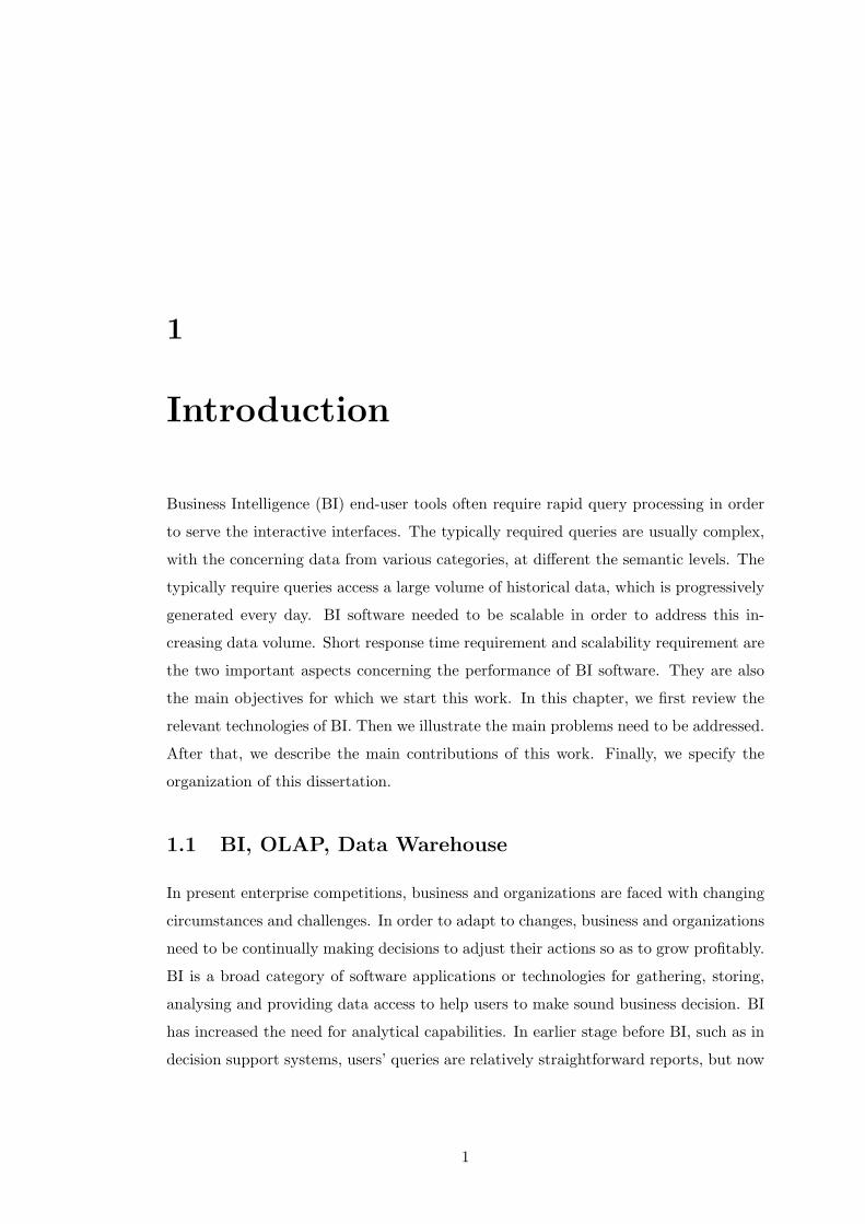
Business Intelligence (BI) end-user tools often require rapid query processing in order
to serve the interactive interfaces. The typically required queries are usually complex,
with the concerning data from various categories, at different the semantic levels. The
typically require queries access a large volume of historical data, which is progressively
generated every day. BI software needed to be scalable in order to address this in-
creasing data volume. Short response time requirement and scalability requirement are
the two important aspects concerning the performance of BI software. They are also
the main objectives for which we start this work. In this chapter, we first review the
relevant technologies of BI. Then we illustrate the main problems need to be addressed.
After that, we describe the main contributions of this work. Finally, we specify the
organization of this dissertation.
1.1 BI, OLAP, Data Warehouse
In present enterprise competitions, business and organizations are faced with changing
circumstances and challenges. In order to adapt to changes, business and organizations
need to be continually making decisions to adjust their actions so as to grow profitably.
BI is a broad category of software applications or technologies for gathering, storing,
analysing and providing data access to help users to make sound business decision. BI
has increased the need for analytical capabilities. In earlier stage before BI, such as in
decision support systems, users’ queries are relatively straightforward reports, but now
1

1. INTRODUCTION
their queries often require on-line analytical capabilities, such as forecasting, predictive
modeling, and clustering.
On-Line Analytical Processing (OLAP) provides many functions which make BI
happens. It transforms data into multidimensional cubes, provides summarized, pre-
aggregated and derived data, manages queries, offers various calculation and modeling
functions. In the BI architecture, OLAP is a layer between Data Warehouse and BI
end-user tools. The results calculated by OLAP are feed to end-user BI tools, which in
turn realize functions like, business modeling, data exploration, performance reporting
and data mining etc. During the data transformation, the raw data is transformed
into multidimensional data cube, over which OLAP processes queries. Thus, answering
multidimensional analytical queries is one of the main functions of OLAP. Codd E.F.
put the concept of OLAP forward in (41), where Codd and his colleagues devised twelve
rules covering key functionality of OLAP tools.
Data Warehouse is an enterprise level data repository, designed for easily reporting
and analysis. It does not provide on-line information; instead, data are extracted from
operational data source, and then cleansed, transformed and catalogued. After such
a set of processing, manager and business professionals can directly use this data for
on-line analytical processing, data mining, market research and decision support. This
set of processing is also considered as the typical actions performed in Data Warehouse.
Specifically, actions for retrieving and analysing data, actions for extracting, transform-
ing and loading data, and actions for managing data dictionary make up the principal
components of Data Warehouse.
1.2 Issues with Data Warehouse
As data is getting generated from various operational data source, the volume of data
stored in Data Warehouse is ever-increasing. While today’s data integration technolo-
gies make it possible to rapidly collect large volume of data, fast analysis over a large
data set still needs the scalability performance of Data Warehouse to be further im-
proved. Scaling up or scaling out with increasing volume of data is the common sense of
scalability. Another aspect of scalability is scaling with increasing number of concurrent
running queries. Comparing with data volume scalability, query number scalability is
relatively well resolved in present Data Warehouse.
2

1.3 Objectives and Contributions
With BI end-user tools, the queries are becoming much more complex than before.
Users used to accept simple reporting function, which involves small volume of aggre-
gated data stored in Data Warehouse. But today’s business professionals demand to
access data from the top aggregate level to the most detailed level. They play more
frequently with Data Warehouse with the ad hoc queries, interactive exploration and
reporting. Interactive interface of BI strictly requires the response time should not be
above 5 seconds, ideally within hundred of milliseconds. Such a short response time
(interactive processing) requirement is another issue with Data Warehouse.
1.3 Objectives and Contributions
In this work, we are going to address data scalability and interactive processing issues
arose in Data Warehouse, and propose a feasible, cheap solution. Our work is aiming
to utilize commodity hardware. Different from those solutions relying on high-end
hardware, like SMP server, our work is realized on commodity computers connecting in
a shared-nothing mode. However, regarding to performance and stability of commodity
hardware and those of high-end hardware are not comparable. The failure rate of
commodity computers is much higher than high-end hardware.
Google proposed MapReduce is the de facto the Cloud computing model. After
the MapReduce article (47) publication in 2004, MapReduce attracts more and more
attentions. For our work, the most attractiveness of MapReduce is its automatical
scalability and fault-tolerance. Therefore, we adopted MapReduce in our work to par-
allelize the query processing. MapReduce is also a flexible programming paradigm. It
can be used to support all of data management processes performed in Data Warehouse,
from Extract, Transform and Load to data cleansing and data analysis.
The major contributions of this work are the following:
• A survey of existing work for accelerating multidimensional analytical
query processing. Three approaches are involved, including pre-computing,
data indexing and data partitioning. These approaches are valuable experience,
from which we can benefit in new data processing scenario. We summarize a wide
range of commonly used operators’ parallelizations.
3
1. INTRODUCTION
• Latency comparison between Hadoop and GridGain. Those are two open-
source MapReduce frameworks. Our comparison shows Hadoop has long latency
and is suitable to for batch processing, while GridGain has low latency, and
is capable of processing interactive query. We chose GridGain because of its
advantage of low latency in the subsequent work.
• Communication cost analysis in MapReduce procedure. MapReduce
hides the communication detail in order to provide an abstract programming
model for developer. In spite of this, we are still curious of the underlying com-
munication. We analysed the communication cost in the MapReduce procedure,
and discussed the main factors affecting the communication cost.
• Proposition and use of manual supporting MapReduce data accessing.
Distributed File System, such as Google File System and Hadoop Distributed File
System and the file system based on cache are two main data storage approaches
used by MapReduce. We propose the third MapReduce data accessing support ,
i.e. manual support. In our work, we use this approach to works with GridGain
MapReduce framework. Although this approach requires developers to take care
of data locating issue, it provides chances for restructuring data, and allows to
improve data access efficiency.
• Making GridGain to support Combiner . Combiner is not provided in
GridGain. For enabling Combiner in GridGain, we propose to combine two
GridGain’s MapReduce tasks to create one MapCombineReduce task.
• Multiple Group-by query implementation basing on MapReduce We
implement MapReduce model and MapCombineReduce based Multiple Group-by
query. A detailed workflow analysis over the GridGain MapReduce procedure has
been done. Speed-up and scalability performance measurement was performed.
Basing on this measurement, we formally estimated the execution time.
• Utilize data restructure improves data access efficiency In order to accel-
erate Multiple Group-by query processing, we first separately partition data with
horizontal partitioning and vertical partitioning. Then, we create index and com-
pressed data over data partitions to improve data access efficiency. These mea-
4
1.4 Organisation of Dissertation
sures result in significant accelerating effects. Similarly, we measure the speed-up
performance of Multiple Group-by query over restructured data.
• Performance affecting factors analysis We summarize the factors affecting
execution time and discuss how they affect the performance. These factors are
query selectivity, number of mappers on one node, hitting data distribution, inter-
mediate output size, serialization algorithms, network status, use or not combiner,
data partitioning methods.
• Execution time modelling and parameters’ values estimation Taking into
account the performance affecting factors, we model the execution time for differ-
ent stage of MapReduce procedure in GridGain. We also estimate the parameters’
value for horizontal partitioning-based query execution.
• Compressed data structure supporting distinct-value-wise job-scheduling
Data location-based job-scheduling is not flexible enough. A more flexible job-
scheduling in our context is distinct-value-wise job-scheduling, i.e. one mapper
works to compute aggregates for only several distinct values of one Group-by di-
mension. We propose a new structure of compressed data, which facilitate this
type of job-scheduling.
1.4 Organisation of Dissertation
The rest of this dissertation is organized as follows.
Chapter 2 focuses on traditional technologies for optimizing distributed parallel
multidimensional data analysis processing. Three approaches for accelerating multi-
dimensional data analysis query’s processing are pre-computing, indexing techniques
and data partitioning. They are still very useful for our work. We will talk about
these three approaches for accelerating query processing as well as their utilizations in
distributed environment. The parallelism of various operators, which are widely used
in parallel query processing, is also addressed.
Chapter 3 addresses data intensive applications based on MapReduce. Firstly, we
will describe the logic composition of MapReduce model as well as its extended model.
The relative issues about this model, such as MapReduce’s implementation frameworks,
cost analysis will also be described. Secondly, we will talk about the distributed file
5

1. INTRODUCTION
system underlying MapReduce. A general presentation on data management applica-
tions in the cloud is given before the discussion about large-scale data analysis based
on MapReduce.
Chapter 4 describes MapReduce-based Multiple Group query processing, one of
our main contributions. We will introduce Multiple Group-by query, which is the calcu-
lation that we will parallelize relying on MapReduce. We will give two implementation
of Multiple Group-by query, one is based on MapReduce, and the other is based on
MapCombineReduce. We also will present the performance measurement and analysis
work.
Chapter 5 talks about performance improvement, one of our main contributions.
We will first present the data restructure phase we adopted for improving performance
of individual job. Several optimizations were performed over raw data set within data
restructuring, including data partitioning, indexing and data compressing. We will
present the performance measurement and the proposed execution time estimation
model. We will identify the performance affecting factors during this procedure. A
proposed alternative compressed data structure will be described at the end of this
work. It enables to realize more flexible job scheduling.
6

2
Multidimensional Data Analyzing
over Distributed Architectures
Multidimensional data analysis applications are largely used in BI systems. Enterprises
generate massive amount of data everyday. These data are coming from various as-
pects of their products, for instance, the sale statistics of a series of products in each
store. The raw data is extracted, transformed, cleansed and then stored under multi-
dimensional data models, such as star-schema1. Users ask queries on this data to help
making business decisions. Those queries are usually complex and involve large-scale
data access. Here are some features we summarized for multidimensional data analysis
queries as below:
• queries accesses large data set performing read-intensive operations;
• queries are often quite complex and require different views of data;
• query processing involves many aggregations;
• updates can occur but infrequently, and can be planned by administrator to
happen at an expected time.
Data Warehouse is the type of software designed for multidimensional data analy-
sis. However, facing to larger and larger volume of data, the capacity of a centralized
Data Warehouse seems too limited. The amount of data is increasing; the number of
concurrent queries is also increasing. The scalability issue became a big challenge for
1A star schema consists of a single fact table and a set of dimension tables
7
2. MULTIDIMENSIONAL DATA ANALYZING OVER DISTRIBUTEDARCHITECTURES
centralized Data Warehouse software. In addition, short response time is also chal-
lenging for centralized Data Warehouse to process large-scale of data. The solution
addressing this challenge is to decompose and distribute the large-scaled data set, and
calculate the queries in parallel.
Three basic distributed hardware architectures exist, including shared-memory,
shared-disk, and shared-nothing. Shared-memory and shared-disk architectures can-
not well scale with the increasing data set scale. The main reason is that these two
distributed architectures all require a large amount of data exchange over the inter-
connection network. However, interconnection network cannot be infinitely expanded,
which becomes the main shortage of these two architectures. On the contrary, shared-
nothing architecture minimizes resource sharing. Therefore, it minimizes the resource
contentions. It fully exploits local disk and memory provided by a commodity com-
puter. It does not need a high-performance interconnection network, because it only
exchanges small-sized messages over network. Such an approach minimizing network
traffic allows more scalable design. Nowadays, the popular distributed systems almost
adopted the shared-nothing architectures, including, peer-to-peer, cluster, Grid, Cloud.
The research work related to data over shared-nothing distributed architectures is also
very rich. For instance, parallel database like Gamma (54), DataGrid project (6),
BigTable (37) etc. are all based on shared-nothing architecture.
In the distributed architecture, data is replicated on different nodes, and query is
processing in parallel. For accelerating multidimensional data analysis query’s pro-
cessing, people proposed many optimizing approaches. The traditional optimizing ap-
proaches, used in centralized Data Warehouse, mainly include pre-computing, indexing
techniques and data partitioning. These approaches are still very useful in the dis-
tributed environment. In addition, a great deal of work is also done for paralleling
the query processing. In this chapter, we will talk about three approaches for accel-
erating query processing as well as their utilizations in distributed environment. We
will present parallelism of various operators, which are widely used in parallel query
processing.
8

2.1 Pre-computing
2.1 Pre-computing
Pre-computing approach resembles the materialized views optimizing mechanism used
in database system. In multidimensional data context, the materialized views become
data cubes1. Data cube stores the aggregates for all possible combination of dimen-
sions. These aggregates are used for answering the forthcoming queries.
For a cube with d attributes, the number of sub-cubes is 2d. With the augment of the
number of cube’s dimensions, the total volume of data cube will exponentially increase.
Thus, such an approach produces data of volume much larger than the original data
set, which might not have a good scalability facing to the requirement of processing
larger and larger data set. Despite this, the pre-computing is still an efficient approach
for accelerating query processing in a distributed environment.
2.1.1 Data Cube Construction
Constructing data cube in a distributed environment is one of the research topics. The
reference (93) proposed some methods for construction of data cubes on distributed-
memory parallel computers. In their work, the data cube construction consists of six
steps:
• Data partitioning among processors.
• Load data into memory as a multidimensional array.
• Generate a schedule for the group-by aggregations.
• Perform the aggregation calculations.
• Redistribute the sub-cubes to processors for query processing.
• Define local and distributed hierarchies on all dimensions.
In the data loading step (step 2), the size of the multidimensional array in each
dimension equals the number of distinct values in each attribute; each record is repre-
sented as a cell indexed by the values2 of each attribute. This step adopted two different
1Data Cube is proposed in (67), it is described as an operator, it is also called for short as cube.Cube generalizes the histogram, cross-tabulations, roll-up, drill-down, and sub-total constructs, whichare mostly calculated by data aggregation.
2The value of each attribute is a member of the distinct values of this attribute.
9
2. MULTIDIMENSIONAL DATA ANALYZING OVER DISTRIBUTEDARCHITECTURES
methods for data loading: hash-based method and sort-based one. For small data sets,
both methods work well, but for large data sets, the hash-based method works better
than the sort-based method, because of its inefficient memory usage1. The cost for
aggregating the measure values stored in each cell is varying. The reason is that the
whole data cube is partitioned over one or more dimensions, and thus some aggregating
calculations involve the data located on other processors. For example, for a data cube
consisting of three dimensions A, B and C, being partitioned over dimension A, then
aggregations for the series of sub-cubes ABC→AB→A involve only local calculations
on each node. However, the aggregations of sub-cube BC need the data from the other
processors.
2.1.2 Issue of Sparse Cube
The sparsity is an issue of data cube storage. In reality, the sparsity is a common
case. Take an example of a data cube consisting of three dimensions (product, store,
customer). If each store sells all products, then the aggregation over (product, store)
produces |product| × |store| records. When the number of distinct values for each
dimension increases, the product of above formula will greatly exceed the number of
records coming from the input relation table. When a customer enters a store, he/she
is not possible to cannot buy 5% of all the products. Thus, many records related to this
customer will be a cell ”empty”. In the work of (58), the authors addressed the problem
of sparsity in multidimensional array. In this work, data cube are divided into chunks,
each chunk is a small equal-sized cube. All cells of a chunk are stored contiguously in
memory. Some chunks only contain sparse data, which are called sparse chunks. For
compressing the sparse chunks, they proposed a Bit-Encoded Sparse Storage (BESS)
coding method. In this coding method, for a cell presents in a sparse chunk, a dimension
index is encoded in ⌈log |di|⌉ bits for each dimension di. They demonstrated that data
compressed in this coding method could be used for efficient aggregation calculations.
2.1.3 Reuse of Previous Query Results
Apart from utilizing pre-computed sub-cubes to accelerate query processing, people
also tried to reuse the previous aggregate query results. With previous query results
1Sort-based method is excepted to work efficiently as in external memory algorithms it reduces thedisk I/O over the hash-based method.
10
2.1 Pre-computing
being cached in memory, if the next query, say Qn, is evaluated to be contained within
one of the previous queries, say Qp, thus Qn can be answered using the cached results
calculated for Qp. The case where Qp and Qn have entire containment relationship
is just a special case. In a more general case, the relationship between Qp and Qn is
only overlapping, which means only part of the cached results of Qp can be used for
Qp. For addressing this partial-matching issue, the reference (51) proposed a chunk-
based caching method to support fine granularity caching, allowing queries to partially
reuse the results of previous queries which they overlap; another work (75) proposed a
hybrid view caching method which gets the partial-matched result from the cache, and
calculates the rest of result from the component database, and then it combines the
cached data with calculated data to form the final result.
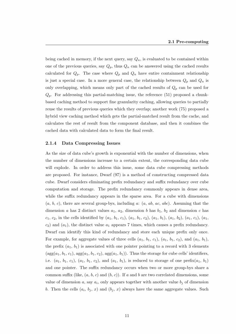
2.1.4 Data Compressing Issues
As the size of data cube’s growth is exponential with the number of dimensions, when
the number of dimensions increase to a certain extent, the corresponding data cube
will explode. In order to address this issue, some data cube compressing methods
are proposed. For instance, Dwarf (97) is a method of constructing compressed data
cube. Dwarf considers eliminating prefix redundancy and suffix redundancy over cube
computation and storage. The prefix redundancy commonly appears in dense area,
while the suffix redundancy appears in the sparse area. For a cube with dimensions
(a, b, c), there are several group-bys, including a: (a, ab, ac, abc). Assuming that the
dimension a has 2 distinct values a1, a2, dimension b has b1, b2 and dimension c has
c1, c2, in the cells identified by (a1, b1, c1), (a1, b1, c2), (a1, b1), (a1, b2), (a1, c1), (a1,
c2) and (a1), the distinct value a1 appears 7 times, which causes a prefix redundancy.
Dwarf can identify this kind of redundancy and store each unique prefix only once.
For example, for aggregate values of three cells (a1, b1, c1), (a1, b1, c2), and (a1, b1),
the prefix (a1, b1) is associated with one pointer pointing to a record with 3 elements
(agg(a1, b1, c1), agg(a1, b1, c2), agg(a1, b1)). Thus the storage for cube cells’ identifiers,
i.e. (a1, b1, c1), (a1, b1, c2), and (a1, b1), is reduced to storage of one prefix(a1, b1)
and one pointer. The suffix redundancy occurs when two or more group-bys share a
common suffix (like, (a, b, c) and (b, c)). If a and b are two correlated dimensions, some
value of dimension a, say ai, only appears together with another value bj of dimension
b. Then the cells (ai, bj , x) and (bj , x) always have the same aggregate values. Such
11

2. MULTIDIMENSIONAL DATA ANALYZING OVER DISTRIBUTEDARCHITECTURES
a suffix redundancy can be identified and eliminated by Dwarf during the construction
of cube. Thus, for a cube of 25 dimensions of one petabyte, Dwarf reduces the space
to 2.3 GB within 20 minutes.
The condensed cube (104) is also a work for reducing the size of data cube. Con-
densed cube reduces the size of data cube and the time required for computing the
data cube. However, it does not adopt the approach of data compression. No data
decompression is required to answer queries. No on-line aggregation is required when
processing queries. Thus, there is no additional cost is caused during the query process-
ing. The cube condensing scheme is based on the Base Single Tuple (BST) concept.
Assume a base relation R (A, B, C,...) , and the data cube Cube(A, B,C) is con-
structed from R. Assume that attribute A has a sequence of distinct values a1, a2...an.
Considering a certain distinct value ak, where 1 ≤ k ≤ n, if among all the records of R,
there is only one record, say r, containing the distinct value ak, then r is a BST over
dimension A. To be noted, one record can be a BTS on more than one dimension. For
example, continuing the previous description, if the record r contains distinct value cj
on attribute C, and no else record contains cj on attribute C, then record r is the BST
on C. The author gave a lemma saying that if record r is a BST for a set of dimen-
sions, say SD, then r is also the BTS of the superset of SD. For example, consider
record r, a BST on dimension A, then r is also the BST on (A, B), (A, C), (A, B,
C). The set contains all these dimensions is called SDSET . The aggregates over the
SDSET of a same BST r concern always the same record r, which means that any the
aggregate function aggr() only apply on record r. Thus, all these aggregate values will
have equal value aggr(r). Thus, only one unit of storage is required for the aggregates
of the dimensions and combination of dimension from SDSET .
2.2 Data Indexing
Data indexing is an important technology of database system, especially when good
performance of read-intensive query is critical. The index is composed of a set of
particular data structure specially designed for optimizing the data access. When per-
forming read operations over the raw data set, within which the values of column are
randomly stored, only full table scan can achieve data item lookup. In contrast, when
performing read operations over index, where data items are specially organized, and
12

2.2 Data Indexing
the auxiliary data structures are added, the read operations can be performed much
more efficiently. For queries of characteristics of read-intensive, like multidimensional
data analysis query, index technology is an indispensable aid to accelerate query pro-
cessing. Compared with other operations happening within the memory, the operations
for reading data from the disk might be the most costly operations. One real example
cited from (80) can demonstrate this: ”we assume 25 instructions needed to retrieve
the proper records from each buffer resident page. Each disk page I/O requires several
thousand instructions to perform”. It is clear that data accessing operations are very
expensive. Especially, it becomes the most common operation in the read-intensive
multidimensional data analysis application. Indexing data improves the data access-
ing efficiency by providing the particular data structures. The performance of index
structures depends on different parameters, such as the number of stored records, the
cardinality of the data set, disk page size of the system, bandwidth of disks and latency
time etc. The index techniques used in Data Warehouse is coming from the index of
database. Many useful indexing technologies are proposed, such as, B-tree/B+-tree
index (55), projection index(80), Bitmap index (80), Bit-Sliced index (80), join index
(103), inverted index (42) etc. We will review these interesting index technologies in
this section.
2.2.1 B-tree and B+-tree Indexes
B+-tree indexes(55) are one of the commonly supported index types in relational
database systems. A B+-tree is a variant of B-tree. To this end, we will briefly review
B-tree. The Figure 2.1 illustrates these two types of index. In a B-tree with order of
d, each node has at most 2d keys, and 2d + 1 pointers, but at least d keys and d + 1
pointers. Each node is stored in form of one record in the B-tree index file. Such a
record has a fixed length, and is capable of accommodating 2d keys and 2d+1 pointers
as well as the auxiliary information, specifying how many keys are really contained in
this node. In a B-tree of order d, accommodating n keys, a lookup for a given key never
uses more than 1 + ⌈logd n⌉ visits, where 1 represents the visit of root, ⌈logd n⌉ is the
height of tree, which is also the longest path from root to any leaf. As an example,
the B-tree shown in Figure 2.1 (a) has order d = 2, because each node holds keys of
number between d and 2d, i.e. between 2 and 4. In total, 26 keys reside inside the
13

2. MULTIDIMENSIONAL DATA ANALYZING OVER DISTRIBUTEDARCHITECTURES
B-tree index. Then, a lookup over this B-tree involves no more than 1 + ⌈log2 26⌉ = 3
operations.
B+-tree is an extension of B-tree. In a B+-tree, all keys reside in the leaves, but
the branch part (upper level above the leaves) is actually a B-tree index, except that
the separator keys held by the upper-level nodes still appear in one of their lower-level
nodes. The nodes in the upper-level have different structure from the leaf nodes. The
leaves in a B+-tree are linked together by pointers from left to right. The linked leaves
form a sequence key set. Thus, a B+-tree is composed of one independent index for
search and a sequence set. As all keys are stored in leaves, any lookup in B+-tree
spends visits from the root to a leaf, i.e. 1 + ⌈logd n⌉ visits. An example of B+-tree is
shown in Figure 2.1 (b).
(a)B-tree of order d = 2
(b)B+-tree of order d = 3
Figure 2.1: B-tree index (a) vs. B+-tree index(b)
B+-tree indexes are commonly used in database systems for retrieving records which
contain the given values in specified columns. A B+-tree over one column takes the
distinct values as the keys. In practice, only the prefix of each distinct value is stored in
the branch part nodes, for saving space. On the contrary, the keys stored in the leaves
accommodate distinct values. Each record of a table with a B+-tree index on one
column is referenced once. Records are partitioned by distinct values of the indexed
14
2.2 Data Indexing
column, and the list of RecordIDs indicating those records having the same distinct
value are associated to a same key.
B+-tree indexes are considered to be very efficient for lookup, insertion, and dele-
tion. However, in the reference (80), the author pointed out the limitation of B+-tree
index: it is inconvenient when the cardinality of the distinct values is small. The reason
is that, when the number of distinct values (i.e. keys in B+-tree index) is small com-
pared with the record number, each distinct value is associated with a large number of
RecordIDs. Thus, a long RecordID-list needs to be stored for every key (distinct value).
Assume that one RecordID is stored as an integer, thus it takes 4 bytes for storing one
RecordID. Even after compressing, the space required for storing these RecordIDs can
take up to 4 times space required for stocking all RecordIDs. Therefore, in case of small
number of distinct values, B+-tree indexes are not space-efficient.
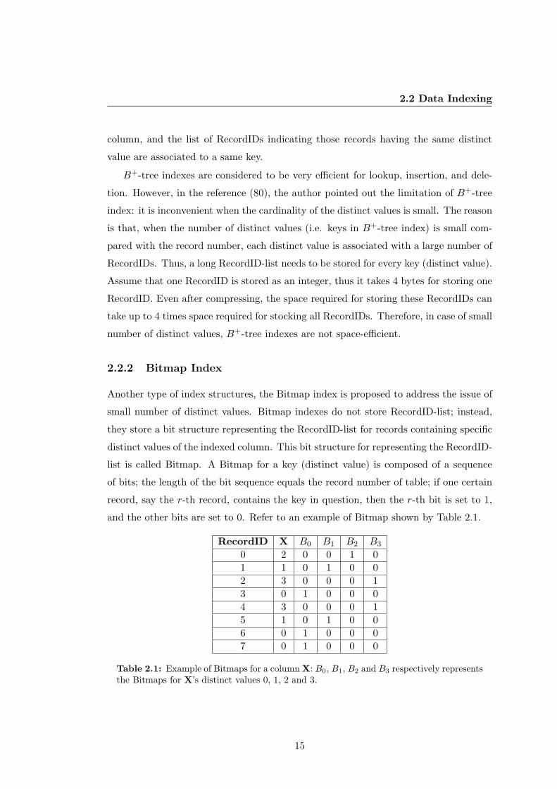
2.2.2 Bitmap Index
Another type of index structures, the Bitmap index is proposed to address the issue of
small number of distinct values. Bitmap indexes do not store RecordID-list; instead,
they store a bit structure representing the RecordID-list for records containing specific
distinct values of the indexed column. This bit structure for representing the RecordID-
list is called Bitmap. A Bitmap for a key (distinct value) is composed of a sequence
of bits; the length of the bit sequence equals the record number of table; if one certain
record, say the r-th record, contains the key in question, then the r-th bit is set to 1,
and the other bits are set to 0. Refer to an example of Bitmap shown by Table 2.1.
RecordID X B0 B1 B2 B3
0 2 0 0 1 0
1 1 0 1 0 0
2 3 0 0 0 1
3 0 1 0 0 0
4 3 0 0 0 1
5 1 0 1 0 0
6 0 1 0 0 0
7 0 1 0 0 0
Table 2.1: Example of Bitmaps for a column X: B0, B1, B2 and B3 respectively representsthe Bitmaps for X’s distinct values 0, 1, 2 and 3.
15

2. MULTIDIMENSIONAL DATA ANALYZING OVER DISTRIBUTEDARCHITECTURES
A Bitmap index for a column C containing distinct values v0,v1,...,vn, is composed
of a B-tree, in which keys are distinct values of C, and each key is associated with a
Bitmap tagging the RecordIDs of records having the current key in its C field. Bitmap
indexes are more space-efficient than storing RecordID-list when the number of keys
(distinct values) is small (80). In addition, as the Boolean operations (AND, OR, Not)
are very fast for bit sequence operands, then operations for applying multiple predicates
are efficient with Bitmap indexes. Similarly, this also requires the indexed column has
a small number of distinct values.
To be noted, storing Bitmaps and storing RecordID-list (used in B-tree and B+-tree)
are two interchangeable approaches. Both of them are aiming to store information of
corresponding RecordIDs for a given distinct value When the number of distinct values
of indexed column is small, each distinct value corresponds to a large number of records.
In this case, the Bitmap is dense i.e. it contains a lot of 1-bits. Therefore, using Bitmap
is more space-efficient. On the contrary, when the number of distinct values is large,
then each distinct value corresponds to a small number of records. In such a case,
directly storing RecordID-list is more space-efficient.
2.2.3 Bit-Sliced Index
Bit-sliced indexes (80) a type of index structure aiming to efficiently access values in
numeric columns. Different from values of ”text” type, numeric values can be extremely
variable, then the number of distinct values can be extremely large too. For indexing a
numeric column, the technologies for indexing text column are not practical. A useful
feature of numeric values is that they can be represented using binary number. In order
to create a bit-sliced index over a numeric column, one need to represent each numeric
value with binary number. Through representing in binary number, one numeric value
is expressed by a sequence of 0 and 1 codes with a fixed length, say N , where the bits in
this sequence are numbered from 0 to N −1. A sequence of Bitmaps, B0, B1 ..., BN−1,
is created, each Bitmap recording the bit values at i-th position (i = 1..N − 1) for all
the column values. Refer to an example of bit-sliced index from Figure 2.2. In this
example, a bit-sliced index is generated for a sale qty column, which stores four data
items of quantity of sold products. These four integer values of sale qty are represented
with binary numbers, each of them having 7 bits. Then these binary numbers are sliced
16

2.2 Data Indexing
into 7 Bitmaps, B0...B6. Bit-sliced indexes can index a large range of data, for instance,
20 Bitmaps are capable of indexing 220 − 1 = 1048575 numeric values.
Figure 2.2: Example of Bit-sliced index
2.2.4 Inverted Index
Inverted index(42) is a data structure which stores a mapping from a word, or atomic
search item to the set of documents, or sets of indexed units containing that word.
Inverted indexes are coming from the information retrieval systems, and widely used
in most full-text search. Search engines also adopted the inverted indexes. After web
pages are crawled, an inverted index of all terms and all pages is generated. Then the
searcher uses the inverted index and other auxiliary data to answer queries. Inverted
index is a reversal of the original text in the documents. We can consider the documents
to be indexed as a list of documents, each document is pointing to a term list. On the
contrary, an inverted index maps terms to documents. Instead of scanning a text and
then seeing its content (i.e. a sequence of terms), an inverted index allows an inverted
search of a term to find its accommodating documents. Each term appears only once in
inverted indexes, but it appears many times in the original documents. The identifier
of document appears many times in inverted indexes, but only once in the original
document list.
An inverted index is composed of two parts, an index for terms and for each term
a posting list (i.e. a list of documents that contain the term). If the index part is
sufficiently small to fit into memory, then it can be realized with a hash table; on
the contrary, if the index part cannot fit into memory, then the index part can be
realized with a B-tree index. Most commonly, B-tree index is used as the index part.
17

2. MULTIDIMENSIONAL DATA ANALYZING OVER DISTRIBUTEDARCHITECTURES
The reference (42) proposed some optimization for B-tree based inverted index. The
optimization involves reducing disk I/Os and storage space. As disk I/Os are the
most costly operations compared with other operations, reducing disk accesses and
reducing storage space also mean accelerating the processing of index creation and
index searching. Two approaches for fully utilizing memories1, i.e. page cache and
buffer, were proposed to create inverted index. With page cache approach, the upper
level part of B-tree is cached in memory, then sequentially read into each word from
documents and write them to the B-tree. In order to update the nodes beyond the
cached part of B-tree, an extra disk access is required. With buffer approach, the
postings reside in a buffer (in memory) instead of the upper level part of B-tree. When
the buffer is full, the postings will be merged with B-tree. During the period of merge,
B-tree’s each sub-tree is iteratively loaded into memory in order to be merged. The
buffer approach is demonstrated to run faster than the page cache approach. Storing
the associated posting list of each term in a heap file on disk can reduce both disk
I/Os and storage space. For reducing the storage space for posting list, a simple delta
encoding is very useful. Instead of storing the locations of all postings as a sequence
of integers, delta encoding just records the distance between two successive locations,
which a smaller integer occupying less space.
In a multidimensional data set, the columns including only pure ”text” type values
are very common. For example, the columns storing information about, city name,
person name, etc. These columns have a limited number of distinct values2. Thus, it is
possible to index values of these ”text” type column with inverted index. To this end,
we consider the column values contained in each record as terms, and the RecordIDs as
a document (i.e. posting in the terminology of full-text search). Instead of storing the
document-ids as the postings, the RecordIDs are stored as postings in inverted index.
Using inverted index allows quickly finding the given term’s locations. Similarly, using
inverted index can quickly retrieve records meeting a query’s condition. The reference
(73) proposed a method of calculating high-dimensional OLAP queries with the help
of inverted indexes. The issue being addressed in this work is the particularly large
number of dimensions in high-dimensional data set. As the number of dimensions are
1Assume that the B-tree index is too large to fit into memory, only a part of nodes of B-tree canreside in memory.
2In contrast, the columns including only numeric type values can have very large number of distinctvalues.
18

2.2 Data Indexing
too large, the data cube is not possible to pre-calculate because of the data cube’s
exponential growth with the number of dimensions. In their work, they vertically par-
titioned the original data set into fragments, each fragment containing a small number
of dimensions. The local data cube is pre-calculated over each fragment instead of over
the original high-dimensional data set. Along with the calculation of local data cubes,
the inverted index for each cuboid1 is also built. The inverted index for a individual
dimension is directly created; the inverted index for non-individual-dimension-cuboid
is calculated by intersecting record-lists of two or more concerned values stored in the
inverted indexes of concerned individual-dimension-cuboids. Here, these inverted in-
dexes are served to efficiently retrieve concerned RecordIDs for computing cells of a
given cuboid.
Lucene(16) is an open-source implementation of inverted index. It is originally cre-
ated by Doug Cutting, one author of the reference (42). It is now under the Apache Soft-
ware License. It is adopted in the implementation of Internet search engines. Lucene
offers a set of APIs for creating inverted index and search on it. Lucene allows user to
reconfigure the parameters to obtain higher performance.
2.2.5 Other Index Techniques
Projection Index
Taking into account that most queries retrieve only a part of columns, accessing the
whole table for reading only part of them is considered to be inefficient. For solving
this problem, projection index is proposed in (80). A projection index over one column
extracts the values of this column from the raw data table, keeping the order of values
as in the ordinal data table. In case of processing query concerning a small number of
columns being concerned, data access over projection indexes is very efficient.
Join Index
Join index (103) is proposed to optimize the join operations. A join index concerns
two relations to be joined. Assuming A and B are two relations to join, and A joins B
1A cuboid is an element composing data cube, and it is also a group-by over the original data set.For example, for a data set with 3 dimensions (A1, A2, A3), the cuboids composing the cube (A1, A2,A3) are: {A1, A2, A3, (A1, A2), (A1, A3), (A2, A3), (A1, A2, A3)}. The cuboid on all dimensions iscalled base cuboid.
19

2. MULTIDIMENSIONAL DATA ANALYZING OVER DISTRIBUTEDARCHITECTURES
will produce a new relation T . Then a join index for two joining relations A and B—
join operation concerns the column a from A and the column b from B—is composed
of columns a and b, each qualified record will appear in the produced relation T. Join
index can be used together with other indexing technologies, such as Bitmap index,
Projection index, Bit-Sliced index. Choosing appropriate combination according to the
characteristics of queries will produce high efficiency (80). For instance, a combination
between Join index and Bitmap index can avoid creating and storing many Join indexes
for all joins probably appear before processing a query, because the join index can be
rapidly created in the runtime with the aid of Bitmap index.
R-tree Index
R-tree index is an index structure similar to B-tree, but is used to access cells of
a multidimensional space. Each node of an R-tree has a variable number of entries
(up to some pre-defined maximal value). Each entry within a non-leaf node stores
two pieces of data: a way of identifying a child node, and the bounding box of all
entries within this child node. Some research work has exploited R-tree index to build
index over data cube, such as Cubetree (92), Master-Client R-Tree (94), and RCUBE
index (48). Cubetree is a storage abstraction of the data cube, which is realized with a
collection of well organized packed R-trees that achieve a high degree of data clustering
with acceptable space overhead. A Master-client tree index is composed of the non-leaf
nodes stored on master and leaf nodes stored on clients; each client builds a complete
R-tree for the portion of data assigned to it. RCUBE index is similar to Master-Client
tree index, except that there is no a global R-tree on a dedicated node (Master), instead,
and the queries are passed in form of messages directly to each processor.
2.2.6 Data Indexing in Distributed Architecture
Using indexing technology in a distributed architecture for efficient query processing is
still an open issue. The challenge is concerning with data partitioning and data ordering
so as to satisfy the requirements of load balancing and minimal disk accesses over each
node. More specifically, load balancing requires reasonably partitioning data set and
placing each data partitions over nodes so that the amount of data retrieved from
20

2.3 Data Partitioning
each node as evenly as possible1; minimal disk accesses requires good data structure to
augment the efficiency of data accessing over the disk of each node.
In the reference (44), the author proposed an index method similar to projection
indexing and join index to process queries. Differently, they use these indexes in a
distributed environment (shared-nothing). This work is based on a star-schema data
set, which is composed of several dimension tables and one fact table. In this work,
the data index is called Basic Data Index (BDI ). BDI is a vertical partition of the
fact table, which includes more than one column. The BDI is separated out and be
stored respectively, having the same number of records as in the fact table. After
separating out one BDI, the fact table does not keep the same columns. Assuming
the star-schema data set has d dimensions, the fact table is vertically partitioned into
d+1 BDI s, which d BDI s storing columns related to d dimensions, and 1 BDI storing
the remaining columns of the fact table. The Join Data Index (JDI ) is designed to
efficiently process join operations between fact table and dimension table. Thus, it
concerns one of BDI s separated from the fact table and one dimension table. A JDI
add to the BDI the corresponding record’s RecordIDs, which identify the record in the
dimension table. In this way, the join operation between fact table and dimension table
can be accomplished with only one scan over JDI.
2.3 Data Partitioning
In order to reduce the resource contention 2, a distributed parallel system often uses
affinity scheduling mechanism; giving each processor an affinity process to execute.
Thus, in a shared-nothing architecture, this affinity mechanism tends to be realized
by data partitioning; each processor processes only a certain fragment of the data set.
This forms the preliminary idea of data partitioning.
Data partitioning can be logical or physical. Physical data partitioning means
reorganizing data into different partitions, while logical data partitioning will greatly
affect physical partitioning. For example, a design used in Data Warehouse, namely
data mart, is a subject-oriented logical data partitioning. In a Data Warehouse built
in an enterprise, each department is interested only in a part of data. Then, the data
1Data partitioning will also be referred to later in this chapter.2Resource contention includes disk bandwidth, memory, network bandwidth, etc.
21

2. MULTIDIMENSIONAL DATA ANALYZING OVER DISTRIBUTEDARCHITECTURES
partitioned and extracted from Data Warehouse for this department is referred as a
data mart. As we are more interested in the physical data access issue, we will focus
on the physical data partitioning techniques.
2.3.1 Data Partitioning Methods
Data partitioning allows exploiting the I/O bandwidth of multiple disks by reading
and writing in parallel. That increases the I/O efficiency of disks without needing any
specialized hardware (52). Horizontal partitioning and vertical partitioning are two
main methods of data partitioning.
2.3.1.1 Horizontal Partitioning
Horizontal partitioning conserves the record’s integrality. It divides tables, indexes
and materialized views into disjoint sets of records that are stored and accessed sepa-
rately. The previous studies show that horizontal partitioning is more suitable in the
context of relational Data Warehouses(33). There mainly are three types of horizontal
partitioning, round-robin partitioning, range partitioning and hash partitioning.
Round-robin partitioning is the simplest strategy to dispatch records among parti-
tions. Records are assigned to each partition in a round-robin fashion. Round-robin
partitioning works well if the applications access all records in a sequential scan. Round-
robin does not use a partitioning key, and then records are randomly dispatched to
partitions. Another advantage of round-robin is that it gives good load balancing.
Range partitioning uses a certain attribute as the partitioning attribute, and records
are distributed among partitions according to their values of the partitioning attribute.
Each partition contains a certain range of values on an indicated attribute. For example,
table CUSTOMER INFO stores information about all customers. We define column
ZIP-CODE as the partition key. We can range-partition this table by giving a rule
as zip-code between 75000 and 75019. The advantages of range partitioning is that it
works well when applications sequentially or associatively access data1, since records
are clustered after being partitioned. Data clustering puts related data together in
physical storage, i.e. the same disk pages. When applications read the related data,
the disk I/Os are limited. Each time one disk page is read, not only the targeted data
1Associative data accessing means access all records holding a particular attribute value.
22

2.3 Data Partitioning
item, but also other needed data items of potential operations are fetched into memory.
Thus, Range partitioning makes disk I/Os more efficient.
Hash partitioning is ideally suitable for applications that access data in a sequen-
tial manner. Hash partitioning also needs an attribute as the partitioning attribute.
Records are assigned to a particular partition by applying a hash function over the
partitioning key attribute of each record. Hash partitioning works well with both se-
quential data access applications and associative data access ones. It can also handle
data with no particular order, such as alphanumeric product code keys.
The problem with horizontal partitioning is that it might cause data skew, where
all required data for a query is put in one partition. Hash partitioning and round-robin
partitioning are less possible to causes data skew, but range partitioning is relatively
easy to cause this issue.
2.3.1.2 Vertical Partitioning
Another data partitioning method is vertical partitioning, which divides the original
table, index or materialized view into multiple partitions containing fewer columns.
Each partition has full number of records, but partial attributes. As each record has
fewer attributes, the size of record is smaller. Thus, each disk page can hold more
records, which allows query processing to reduce disk I/Os. When the cardinality of
the original table is large, this benefit is more obvious.
However, vertical partitioning has some disadvantages. Firstly, updating (insert or
delete) records in a vertically partitioned table involves operations over more proces-
sors. Secondly, vertical partitioning breaks the record integrality. Nevertheless, vertical
partitioning is useful in some specific contexts. For example, it can separate frequently
updated data (dynamic data) columns from static data columns; the dynamic data can
be physically stored as a new table. In the processing of data read-intensive OLAP
queries, vertical partitioning has its proper advantages:
• With isolating certain columns, it is easier to access data, and create index over
these columns (45; 44).
• Column-specific Data compression, like run-length encoding, can be directly per-
formed (24).
23

2. MULTIDIMENSIONAL DATA ANALYZING OVER DISTRIBUTEDARCHITECTURES
• Multiple values from a column can be passed as a block from one operator to the
next. If existing attributes have fix-length values, then they can be iterated as
array (24).
• For some specific data set with a high dimension number, vertical partitioning is
more reasonable in terms of time and space costs (74).
2.3.2 Data Replication
Data replication technique is usually used together with data partitioning. Data repli-
cation is used to increase the liability. Multiple identical copies of data are stored over
different machines. Once the machine holding the primary copy is down, then the data
can still be accessed on machines holding the copies. In general, data replication and
distribution are not necessary together with data partitioning. They are the technolo-
gies can be used alone. In the work of (29), the author proposed an adaptive virtual
partitioning for OLAP query processing based on shared-nothing architecture. In their
approach, the data set is replicated over all the nodes in the shared-nothing cluster.
The virtual partitioning does not physically partition the data set, instead, it creates
a set of sub-queries including different predicates. By applying these predicates, the
original data set is virtually partitioned, the original query is run only on the data
items belonging to the partition.
2.3.3 Horizontally Partitioning Multidimensional Data Set
The multidimensional data set usually has a large volume. But the calculations over
them are expected running rapidly. As one of the OLAP query optimizing approaches,
data partitioning makes it possible to process queries in a parallel and distributed
fashion. Also, it can reduce irrelevant data accesses, improve the scalability, and ease
data management. In this sub-section, we summarize the applications of horizontal
partitioning in OLAP query processing. By horizontal partitioning, we refer to the
partitioning method that conserves the record integrality. According to the ways for
storing data, OLAP tools can be categorized into Relational OLAP (ROLAP) and
Multidimensional OLAP (ROLAP). In ROLAP, data is stored in form of relations
under star-schema. In MOLAP, data is stored in form of cubes or multidimensional
24

2.3 Data Partitioning
arrays i.e. data cubes. We separately specify the data partitioning approaches designed
for these two different data models.
2.3.3.1 Partitioning Multidimensional Array Data
In a MOLAP, data cube is represented as a multidimensional space, stored in opti-
mized multidimensional array storage. In the multidimensional space, each dimension
is represented as an axis; the distinct values of each dimension are various coordinate
values on the corresponding axis. The measures are loaded form each record in the
original data set into the cells of this multidimensional space, each cell being indexed
by the unique values of each attributes of the original record. Partitioning a data cube
into dimensions and measures is a design choice (93).
Partitioning data cubes should support equal or near-equal distributions of work
(i.e. the various aggregate computations for a set of cuboids) among processors. The
partitioning approach should be dimension-aware, which means that it should pro-
vide some regularity for supporting dimension-oriented operations. Partitioning can be
performed over one or more dimensions(93; 58). That is to say, the basic multidimen-
sional array is partitioned on one or more dimensions. The dimensions over which the
partitioning is performed are called partitioning dimensions. After partitioning, each
processor holds a smaller multidimensional array, where the number of distinct values
held in each partitioning dimension is smaller than in the whole multidimensional ar-
ray. Thus, the distinct values over each partitioning dimension are not be overlapped
among the sub-multidimensional arrays held by each processor. In order to obtain the
coarsest partitioning grain possible, the dimension(s) having largest number of distinct
values is chosen to be the partitioning dimension. Assume a data set with 5 attributes
(A, B, C, D, M ), among them A, B, C, D are the dimensions (axis) in the multidi-
mensional array, and M is the measure stored in each cell of multidimensional array.
Da, Db, Dc and Dd are number of distinct values in each dimension, respectively, with
Da ≥ Db ≥ Dc ≥ Dd established. This data set will be partitioned and distributed over
p processors, numbered P0...Pn−1. Thus, an one-dimension partitioning will partition
on A, since the A has the biggest number of distinct values1; this partitioning also
builds an order on A, which means if Ax ∈ Pi and Ay ∈ Pj then Ax ≤ Ay for i < j.
1Similarly, a two-dimension partitioning will partition on A, B, since A and B have the biggestnumber of distinct values.
25
2. MULTIDIMENSIONAL DATA ANALYZING OVER DISTRIBUTEDARCHITECTURES
The sub-cubes are constructed over processors with their local sub-data set (i.e.
partition). In order to guarantee that each partition does not have overlaps over the
partitioning dimension’s distinct values, the sampling-like record distributing methods,
such hash-based or sort-based method can be used to distribute records to various
processors as described in (93).
Constructing the sub-cube is performed by scanning sub-data set attributed to the
local processor. In reference (93), the sub-data-set is scanned twice. The first scan
obtains the distinct values for each dimension contained in the sub-data-set, and con-
structs a hash-table for various dimensions’ distinct values. The second scan loads the
records into the multidimensional array. Record loading (the second scan) works to-
gether with probing the hash-tables created earlier. During this process, the method
chosen for partitioning and distributing the original data set, will affected the perfor-
mance because the way to access data is slightly different.
Another thing to be noted is that data partitioning determines the amount of data
movement during the aggregates’ computations of the aggregates (58). As the com-
putations of various cuboids involve multiple aggregations over any combination of
dimensions, some cuboid computations are non-local. They need to newly partition
over a dimension and distribute the partitions. Assume that the multidimensional ar-
ray of the 4 dimensional cube is partitioned over A, B, then the aggregation of over
dimension C from ABC1 to AC involves aggregations over dimension B, and requires
partitioning and distribution over dimension C.
2.3.3.2 Partitioning Star-schema Data
In ROLAP, data is organized under star-schema. Horizontal partitioning was considered
an effective method compared to vertical partitioning for star schema data (70). In the
centralized Data Warehouse, data is stored in form of star schema. In general, star
schema is composed of multiple dimension tables and one fact table. Since horizontal
partitioning addresses the issue of reducing irrelevant data access, it is helpful to avoid
unnecessary I/O operations. One of the features about data analysis queries run on
Data Warehouse is they involve multiple join operations between dimension tables and
the fact table. The derived horizontal partitioning, developed for optimizing relational
database operations, can be used to efficiently processed these join operations.
1The letters with underlines represents the dimensions being partitioned and distributed.
26

2.3 Data Partitioning
Partitioning only fact table
This partitioning scheme partitions only the fact table, and replicating the dimension
tables, since the fact table is generally large.
The reference (34) proposed stripping-partitioning approach. In this approach, the
dimension tables are fully replicated over all compute nodes without being partitioned,
as they are relatively small. The fact table is partitioned using round-robin partitioning
and each partition is distributed to a compute node. Defining N as the number of
computers, each computer stores 1/N fraction of total amount of records. Records
of fact table are striping-partitioned by N computers, then queries can be executed
in parallel. In this way, they guaranteed a nearly linear speed-up and significantly
improvement of query response time.
The size of each partition determines the workload attributed to a processor. The
partition size needs to be tuned according to variant queries. A virtual partitioning
method (28) was proposed for this purpose. It allows greater flexibility on node alloca-
tion for query processing than physical data partitioning. In this work, the distributed
Data Warehouse is composed of several database systems running independently. Data
tables are replicated over all nodes, and each query is broken into sub-queries by ap-
pending range predicates specifying an interval on the partitioning key. Each database
system receives a sub-query and is forced to process a different subset of data of the
same size. However, the boundaries limiting each subset are very hard to compute, and
dispatching the one sub-query per node makes it difficult to realize dynamic load bal-
ancing. A fine-grained virtual partitioning (FGVP) (31) was proposed addressing this
issue. FGVP decomposes the original query into a large number of sub-queries instead
of one query per database system. It avoids fully scanning table and suffers less from
the individual database system internal implementation. However, determining appro-
priate partition size is still difficult. Adaptive Virtual Partitioning (AVP) (29) adopted
an experimental approach to obtain the appropriate partitioning size. An individual
database system process the first received sub-query with a given small partitioning
size. Each time it starts to process a new sub-query, it increases the partitioning size.
This procedure repeats until the execution time does not shorten any more, then the
best partitioning size is found. Performing AVP needs some metadata information.
Metadata information includes clustered index of the relations, names and cardinalities
of relations, attributes on which a clustered index is built, the range of values of such
27
2. MULTIDIMENSIONAL DATA ANALYZING OVER DISTRIBUTEDARCHITECTURES
attributes. The meta data information is stored in a catalog in the work of (69).
Partitioning dimension tables & fact table
This partitioning scheme works with star-schema is partitions both dimension tables
and fact table. Often, the dimension tables are horizontally partitioned into various
fragments, and the fact table is also horizontally partitioned according to the parti-
tioning results of dimension tables. This scheme takes in to account of the star-join
requirements.
The number of the fact table partitions depends on the partition number of each
dimension table. Assume N is the number of fact table partitions, p1...pd are the
partition numbers of dimension tables 1...d. If fact table partitioning considers all
partitioning performed on the dimension table, then N = p1 × ... × pd. That means,
along with augment of p1...pd, N will explosively increase. The work of (32) focus on
finding the optimal number of fact table partitions, in order to satisfy two objectives:
• avoid an explosion of the number of the fact table partitions;
• ensure a good performance of OLAP queries.
A generic algorithm is adopted for selecting an horizontal schema in their work.
2.3.4 Vertically Partitioning Multidimensional Data set
Multidimensional data set usually contains many attributes. With the entire record
being stored on the disk (in case of horizontal partitioning), the data access over mul-
tidimensional data set may become inefficient, even though some indexing technique,
like B-tree applied on it. Vertical partitioning is needed in some special cases. Imagine
the following extreme scenario where a query scans only the values of one particular
attribute of each record. Clearly, in this case, scanning the required attribute sepa-
rately is much more efficient than scanning the whole table. From the literature, we
summarized two types of data set, for which vertical partitioning is very suitable, high
dimension data set and read-oriented data set.
The advantages of vertical partitioning versus horizontal one are, firstly, it can
reduce the dimensionality, which in turn enhance the data accessibility; secondly, it
28
2.3 Data Partitioning
enables a set of optimization, like index and compressing easily, to be performed, which
in turn improves the efficiency.
2.3.4.1 Reducing Dimensionality by Vertical Partitioning
In a data set with high dimensionality, the number of dimensions is very large, but
the number of records is moderate. The queries run over such data set concerns only
several dimensions. Although OLAP queries involve high-dimension space, retrieving
data of all dimensions occurs very rarely. Based on this, the authors of reference (74)
employed a vertically partitioning method in their work. They vertically partitioned
the data set into a set of disjoint low dimensional data sets, called fragment. For
each fragment, the local data cube is calculated. These local data cubes are on-line
assembled when queries concerning multiple fragments need to be processed. In this
work, an inverted index based indexing technique and data compressing technique are
applied for accelerating the on-line data cube assemblage1.
2.3.4.2 Facilitating Index and Compression by Vertical Partitioning
In a vertically partitioned data set, data is stored in a column-oriented style. Dif-
ferent from the row-oriented storage where, records are stored one after another, in
the column-oriented storage, attribute values belonging to the same column stored
contiguously, compressed, and densely packed (26). OLAP applications are generally
read-intensive, where the most common operation is to read data from disk, the up-
date operation also occurs, but not frequently. For such read-intensive applications,
the most important performance-affecting factor is the I/O efficiency.
For a multidimensional data set, the traditional indexing techniques, such as B-tree
indexing, are not appropriate. Simply scanning the vertically partitioned data tables
is often more efficient than using B-tree based indexes to answer ad hoc range queries
(100). Using the traditional indexing techniques to process queries involving only a
subset of attributes suffers from the high dimensionality of the data set, since the size
of index increase super-linearly with the augment of the dimension number. With
the vertical partitioning method, the high dimensionality issue is resolved. However,
facing the new data storage structure, not all the traditional indexing techniques are
1Refer to 2.2.4 Inverted index for more information.
29
2. MULTIDIMENSIONAL DATA ANALYZING OVER DISTRIBUTEDARCHITECTURES
appropriate. Bitmap index data structure is mostly used for answering read-intensive
OLAP queries (38), but not optimized for insert, delete or update operations. Having
this characteristic, Bitmap is considered to be the most suitable index for working
with vertical partitioned data. For large data set, Bitmap index can have millions
to billions of bits. It is imperative to compress bitmap index. The authors of (100)
have compared some of the compression schemes such as Byte-aligned Bitmap Code
(BBC), Word-Aligned Hybrid run-length code (WAH), and Word-aligned Bitmap Code
(WBC). They found that WAH is the most efficient in answering queries because it is
much more CPU-efficient.
Compared to row-oriented storage, column-oriented storage presents a number of
opportunities to improve performance by compression techniques. In such a column-
oriented storage, compression schemes encoding multiple values within one time are
natural. For example, many popular modern compression schemes, such as Run-length
encoding, make use of the similarity of adjacent data to compress. However, in a row-
oriented storage system, such schemes do not work well, because an attribute is stored
as a part of an entire record. Compression techniques reduces the size of data, thus it
improves the I/O performance in the following ways (23):
• In a compressed format, data is stored nearer to each other, the seek time is
reduced;
• The transfer time is reduced also because there is less data to be transferred;
• The buffer hit rate is increased because a larger fraction of retrieved data fits in
the buffer pool.
Especially, compression ratios are usually higher in column-oriented storage because
consecutive values of a same column are often quite similar to each other.
2.4 Query Processing Parallelism
Parallelizing query processing over partitioned data set using multiple processors can
significantly reduce the response time. The query processing parallelism has shown
a good speed-up and scale-up for OLTP query, it is worthwhile to investigate paral-
lelism research for processing OLAP query. In the sequential database systems, such
30
2.4 Query Processing Parallelism
as relational database system, queries are often parsed into graphs during the process-
ing. These graphs are called query execution plan or query plan, which is composed of
various operators.
A lot of parallel query processing work has been done in parallel database machines,
such as Gamma (54), Bubba (35), Volcano (59) etc. The main contributions of their
work were parallelization of data manipulations and design of the specific hardware.
Even though parallel database machines were not really put into use, they leaded
database technology toward a good direction, and its research work became the basis
of parallel query processing techniques. The general description of query processing
parallelization is as follows: a query is transformed into N partial queries that are
executed in an independent way in each of N computers. Generally, we can distribute
the same query to all computers, but some types of queries require rewriting.
2.4.1 Various Parallelism Forms
There exist several forms of parallelism that are interesting to designers and imple-
menters of query processing systems (60). Inter-query parallelism means multiple
queries are processed concurrently. For example, several queries contained in a trans-
action are executed concurrently in a database management system. For this form
of parallelism, the resource contention is an issue. Basing on the algebraic operators
parallelization, the parallelism forms can be further refined.
Inter-operator parallelism means parallel execution of different operators in a single
query. It has two sub-forms, i.e. horizontal inter parallelism and vertical inter paral-
lelism. Horizontal inter parallelism means splitting a tree of query execution plan into
several sub-trees, each sub-tree is executed by a processor individually. It can easily
be implemented by inserting a special type of operators, exchange, into the query exe-
cution plan, in order to parallelize the query processing. We will talk about exchange
operator in the following content. Vertical inter-parallelism is also called pipeline, in
which operators are organized into a series of producers and customers. Parallelism is
gained by processing records as a stream. Records being processed by producers are
sent customers. The authors of reference (52) argued that, in a relational database
system, the benefit of pipeline parallelism is limited. The main reasons was: 1) very
long pipelines are rare in query processing based on SQL operators; 2) some SQL oper-
ators do not emit the first item of output until they consumed all items of input, such
31

2. MULTIDIMENSIONAL DATA ANALYZING OVER DISTRIBUTEDARCHITECTURES
as aggregate and sort operators; 3) there often exist one operator which takes much
longer time than other operators, which makes the speed-up by pipeline parallelism be
very limited.
Another form of parallelism is Intra-operator parallelism, which means executing an
operator using several concurrent processes running on different processors. It is based
on data partitioning. The precondition of intra operator parallelism is that query should
focus on sets. Otherwise, if data being queried represents a sequence, for example, time
sequence in a scientific database, then such a parallelism form could not be directly
used, and some additional synchronization should be processed at the result-merging
phase.
2.4.2 Exchange Operator
Exchange operator was proposed in Volcano system (59). It is a parallel operator
inserted into a sequential query execution plan so as to parallelize the query processing.
It is similar to the operators in the system, like open, next, close; other operators are not
affected by the presence of exchange in the query execution plan. It does not manipulate
data. On the logical level, exchange is ”no-op” that has no place in logical query
algebra such as the relational algebra. On the physical level, it provides the ”control”
functions that the other operators do not offer, such as, processes management, data
redistribution, flow control. Exchange provides only ”control” parallelisms, but it does
not determine or presuppose the policies applied for using these mechanisms, such
as degree of parallelism, partitioning functions, attributing processes to processors.
In Volcano, the optimizer or user determines these policies. The Figure 2.3 shows a
parallel query execution plan with exchange operators.
2.4.3 SQL Operator Parallelization
Query running over the partitioned data set can achieve parallelism, which is also called
partitioned parallelism. The algorithms used to implement various operators in parallel
are different from those used in a sequential query execution plan’s implementations.
In the following content, we will summarize the parallelization issues for different op-
erators.
Various SQL operators parallelization algorithms has been introduced in the liter-
ature (52; 60; 68), such as, parallel scan, parallel selection and update, parallel sorting,
32

2.4 Query Processing Parallelism
Figure 2.3: A parallel query execution plan with exchange operators.
parallel aggregation and duplicate removal, parallel join and binary matching. Apart
from these traditionally used SQL operators, some operators specifically designed for
parallel query processing, such as merge, split, are also introduced. We summarize these
algorithms in this section.
2.4.3.1 Parallel Scan
Scan is a basic operator used in query processing. It involves a large number of disk
I/Os, which is also the most expensive operation. Therefore, it is significant to paral-
lelize scan operator in order to share I/O cost. After partitioning data, each parallel
scan operator performs over one partition. The output of parallel scans working over
partitions of a same relation are then processed by a merge operator, which merges
multiple scanning outputs into one output and send it to the application or to the next
operator in the query execution plan.
2.4.3.2 Merge and Split
Merge operator is to collect data. A merge operator is equipped several input ports
and one output port. The input data streams are received at the input ports of merge
33
2. MULTIDIMENSIONAL DATA ANALYZING OVER DISTRIBUTEDARCHITECTURES
operator, and the merging result exits from the output port. If a multi-stage parallel
processing is required, then a data stream need to be split into individual sub-streams.
Split operator serves this purpose. Split is used to partition or duplicate a record
stream into multiple ones. For example, record’s various attributes are sent to different
destination processes through attribute split operator. A split operators partition the
input record stream by applying round-robin, hash partitioning methods, or any other
partitioning methods. Split allows the auto parallelism of new added operators of
system, and it supports various kinds of parallelism.
2.4.3.3 Parallel Selection and Update
Parallel selection operator partitions the workload of selection over several I/O devices,
each being composed of one single disk or an array of disks. Selection operator concur-
rently perform over all required data partitions, and retrieve matching records. If the
partitioning attribute is also the selection attribute, then all disks holding partitions
will not contain the selection results. Thus, the numbers of processes and that of acti-
vated disks are limited. Local index can still bring high efficiency for parallel selection
operator.
Data movement could be caused by update operator in the case of updating the value
of the partitioning attribute of one record. The modified data might need to be moved
to a new disk or node in order to maintain the partitioning consistency. Since moving
data is expensive operation, it is more practical to choose an immutable attribute as
the partitioning attribute in case where the original data set contains dynamic data.
2.4.3.4 Parallel Sorting
Sorting is one of the most expensive operators in database systems. Lots of research
has addressed parallel sorting. Without loss of generality, assume a parallel sorting
operator with multiple inputs and multiple outputs, and further, assume records are
aligned in a random order on the sorting attribute in each input, and the output has
to be range-partitioned with records being sorted within each range. The algorithms
implementing Parallel sorting generally include two phases, local sorting phase and
data exchange phase. In the local sorting phase, records are sorted within multiple
processes. In the data exchange phase, records are sent to a set of processes. The
target process, to which a record is sent, will produce an output partition with the
34
2.4 Query Processing Parallelism
range of sorting attribute value comprising the record’s sorting attribute value. In
other words, the sent records should contribute to the output produced by the target
process. In practice, we can first run data exchange, then local sorting; or, run local
sorting first, then data exchange. If data exchange runs first, then the knowledge of
quantile should be available in order to ensure load balancing. If local sorting runs first,
records are sent, at the end of local sorting, to the right receiving processes, according
to the range that each sent record’s sorting attribute value belongs to.
One of the possible problems during this procedure is deadlock. The reference (60)
summarized the five necessary conditions of deadlock, cited as follows, i.e. if all these
conditions establish, then deadlock will occur. Assume that a couple of parallel sort
operators play with other operators in a relationship of producers and consumers, then
the necessary conditions of deadlock are:
• multiple consumers feed multiple producers;
• each producer produces a sorted stream and each consumer merges multiple sorted
streams;
• some key-based partitioning rule (i.e., hash partitioning) is used other than range
partitioning, ;
• flow control is enabled;
• the data distribution is particularly unfortunate.
Deadlock can be avoided by guaranteeing one of the above conditions does not es-
tablish. Among them, the second condition—each producer produces a sorted stream
and each consumer merges multiple sorted streams—is most easily to be avoided. For
instance, if the sending process (producer) does not perform sorting, or each individ-
ual input stream of receiving process (consumer) is not sorted, then deadlock can be
avoided. That is, moving the sorting operation from producer operator to consumer
operator can resolve deadlock problem.
Deadlocks can also occur during the execution of a sort-merge-join, and they can
be similarly avoided by moving the sorting operation from the producer operator to the
consumer operator. However, this happens when the sorting operation is not possible
to be moved from producer (sort) to consumer (merge-join), for example, reading data
35
2. MULTIDIMENSIONAL DATA ANALYZING OVER DISTRIBUTEDARCHITECTURES
from a B-tree index makes the records being sorted when they are retrieved from
disk. In such a case, it is necessary to find alternative methods that do not require re-
partitioning and merging of sorted data between the producers and consumers. The first
alternative method is moving the consumer’s operations into the producer. Assume the
original data is sorted and partitioned with range- or hash-partitioning method, with
the partitioning attribute being exactly the attribute considered by the operations
of consumer process, e.g. join attribute in case of consumer operator being merge-
join, then the process boundaries and data exchange can entirely be removed from
consumer. This means producer operator, i.e. B-tree scan and consumer operator,
i.e. merge-join, are all performed in a same group of processes. The second method
utilizes fragment-and-replicate to perform join operation. Assume that records of input
stream are sorted over a relevant attribute within each partition, but partitioned either
round-robin or over a different attribute. For such a data distribution, fragment-and-
replicate strategy is applicable. During the join operation with fragment-and-replicate
strategy, one input of join is partitioned over multiple processes and another input of
join is replicated across these processes1. The join operations are running within the
same processes as the processes producing sorted output. Thus, the sorting and join
operations are running in one operator, and deadlocks can be avoided.
2.4.3.5 Parallel Aggregation and Duplicate Removal
There are three commonly used methods for parallelizing aggregation and duplicate
removal. Centralized Two Phase method first does aggregations on each of the mul-
tiprocessors over the local partition, then the partial results are sent to a centralized
coordinator node, which merges these partial results and generates the final result.
Two Phase method parallelizes the processing of the second phase of the Centralized
Two Phase method. The third method is called Re-partitioning. It first redistributes
the relation on the group by attributes, and then it does the aggregation and generates
the final results in parallel over each node. Shatdal et al. (96) argued that those three
methods do not work well for all queries. Both of the Two Phase methods only work
well when the number of result records is small. On the contrary, the Re-partitioning
method works well only when the number of distinct values of group-by attributes is
1In typical fragment-and-replicate join processing, the larger input is partitioned, and the smallerinput is replicated.
36
2.4 Query Processing Parallelism
large. They proposed a hybrid method that changes/decides the method according to
the workload and the number of the distinct values of group-by attributes being com-
puted. A bucket overflow optimization of Two Phase methods was discussed in (60).
For hash-based aggregation, a special technique to improve performance is that they do
not create the overflow file1, and the records can be directly moved to the final nodes,
because in resent shipping records to other node is faster than writing record into disk.
The disk I/O operations are caused when the aggregate output is too large to fit into
memory.
2.4.3.6 Parallel Join
Join operators include different kinds of join operators, which are realized in different
approaches. For instance, semi-join, outer-join, non-equi-join etc. are all join opera-
tors. Different from above mentioned operators, join operators are binary operators,
which involve two inputs.
Executing distributed join operator in parallel indispensably involves send and re-
ceive operation. These operations are based on protocols like TCP/IP or UDP. Row
blocking is a commonly used technique for shipping records to reduce cost. Record
shipping is done in a block-wise way. Instead of being shipped one by one, records are
shipped block by block. This method compensates for the brute in the arrival of data
up to a certain point (68).
Parallel joins over horizontally partitioned data can be achieved by multiple ways.
Assuming relation R is partitioned into R1 and R2: R = R1⋃
R2, then the join between
relations R and S can be computed by (R1⋃
R2) ⋊⋉ S or (R1⋃
S) ⋊⋉ (R2⋃
S). If R is
partitioned into 3 partitions, and S is replicated, then more methods can be adopted.
For instance, the join can be calculated by ((R1⋃
R2) ⋊⋉ S)⋃
(R3 ⋊⋉ S)), with one
replica of S is placed near to R1 and R2, another replica of B is placed near to R3. If
Ri ⋊⋉ Sj is estimated to be, then this partial calculation can be removed to reduce the
overhead.
Sort-merge-join is a conventional method for computing joins. Assume still R and S
are two input relations for join. In sort-merge-join method, both of the input relations
are first sorted over the join attribute. Then these two intermediate relations sorted
are compared, and the matching records are output. Hash-join is an alternative of
1Overflow file means the common overflowing zone of hash table.
37
2. MULTIDIMENSIONAL DATA ANALYZING OVER DISTRIBUTEDARCHITECTURES
sort-merge-join. Hash-join breaks a join into several smaller joins. The two input
relations R and S are hash-partitioned on the join attributes. One partition of relation
R is hash into memory, the related partition of relation S is scanned. Each of the
records in this S partition is compared against the partition of R held in memory.
Once a record is matched, it is outputed. Double-pipelined-hash-join improved the
conventional hash-join. It is a symmetric, incremental join. Double-pipelined-hash-join
creates two in-memory hash-tables, each for one of the input relations. Initially, both
hash-tables are empty. The records of R and S are processed one by one. For processing
one record of R, the hash-table of S is probed, if the record is matched records, then
it is outputed immediately. Simultaneously, the record is inserted into the hash-table
of R for matching the unprocessed records of S. Thus, at any point in time, all the
encountered records are joined. Double-pipelined-hash-join has two advantages. Firstly,
it allows delivering the first results of a query as early as possible. Secondly, it makes it
possible to fully exploit pipelined parallelism, and in turn reduce the overall execution
time.
Symmetric partitioning and fragment-and-replicate are two basic techniques for par-
alelizing binary operators. In symmetric partitioning, both of the inputs are partitioned
over the join attribute, and then the operations will be run on every node. This method
is used in Gamma(54). In fragment-and-replicate method, one of the two inputs is par-
titioned; the other input is broadcasted to all other nodes. In general, the larger input
is partitioned in order not to move it. This method is realized in the early database
systems, because the communication cost overshadowed the computation cost. Send-
ing small input to a small number of nodes costs less than partitioning both larger
input and small input. To be noted, fragment-and-replicate cannot correctly work for
semi-join, and other binary operators, like, difference union, because when a record is
replicated, it will contribute multiple times to the output.
Semi-join is used to process join between relations placed on different nodes. As-
sume two relations R and S are placed on nodes r and s, respectively. Semi-join sends
the needed columns for join of relation R from node r to s, then finds the records qual-
ifying the join from relation S and sends these records back to r. The join operation
is executed on node r. Semi-join can be expressed as: R ⋊⋉ S = R ⋊⋉ (S ⋉π (R)).
Redundant-semi-join is a technique for reducing network traffic used in distributed
38
2.4 Query Processing Parallelism
databases for join processing. This method is used in distributed memory parallel sys-
tems. Assume two relations R and S having a common attribute A, are each stored
on nodes r and s separately. Redundant-semi-join sends the duplicate-free projection
on A to s, executes a semi-join to decide which records of S will contribute to the
join result, and then ships these records to r. Basing on the law of relational algebra
R ⋊⋉ S = R ⋊⋉ (S ⋉ R), there is no need of shipping S, which reduces communication
overhead, at the cost of adding the overhead of projecting, shipping the column A of
R and executing the semi-join. Such a reduction can be applied on R or S, or both
of them. The operations included during this process, such as projection, duplicate
removal, semi-join and final join can be parallelized not only on nodes s and r, but
also on more than two nodes.
Symmetric fragment-and-replicate is proposed by Stamos et al. (98) which is appli-
cable for non-equi-joins and N-way-join. For parallelizing a non-equi-join, processors
are organized into rows and columns. One input relation is partitioned over rows, and
its partitions are replicated over each processor row. The other input relation is par-
titioned over columns, and its partitions are replicated over each processor column. A
record of one input relation only matches with one record from the other input relation.
The global join result is the concatenation of all partial results. This method improves
fragment-and-replicate method by reducing the communication cost.
For joins in a parallel Data Warehouse environment, the parallel star-join is dis-
cussed by Datta et al. in (44). This parallel join processing is based on a special
data structure, Data Index 1, proposed in the same work. Recall that Basic DataIndex
(BDI ) is simply a vertical partition of the fact table, which may include more than one
column and the Join DataIndex (JDI ) is designed to efficiently process join operations
between fact table and dimension table. JDI is an extension of BDI. JDI is composed
of BDI and a list of RecordIDs indicating the matching records in the corresponding
dimension table. Assume that F represents the fact table, and D represents the set
of dimension tables, then | D |= d, which means that there are d dimension tables.
Let G represents a set of processor groups, and | G |= d + 1. Dimension table Di and
the fact table partition JDI corresponding to the key value of Di are distributed to
the processor group i. And the fact table partition BDI after containing measures is
1DataIndex is discussed in section 2.2.6
39

2. MULTIDIMENSIONAL DATA ANALYZING OVER DISTRIBUTEDARCHITECTURES
distributed to processor group d+1. Basing on the above data distribution, the parallel
star-join processing involves only rowsets and projection columns.
In (101) a more complex join operator General Multiple Dimension Join (GMDJ)
is discussed in a distributed Data Warehouse environment. GMDJ is a complex OLAP
operator being composed of relational algebraic operators and other GMDJ opera-
tors. These GMDJ operator-composed queries need a multi-round processing. GMDJ
operator clearly separates group-by definition and aggregate definition, which allows
expressing various kinds of OLAP queries. An OLAP query expressed in GMDJ ex-
pressions is translated into a multi-rounded query plan. During each round, each site
of distributed Data Warehouse executes calculations and communicates its results with
the coordinator; the coordinator synchronize the partial results into a global result, then
transfer the global result to distributed Data Warehouse sites. When a distributed Data
Warehouse site receives an OLAP query, it transforms the OLAP query into GMDJ
operators, then these operators are optimized using distributed computation. Taking
the efficiency into account, the synchronization at the end of each round is started when
the faster sites’ partial results arrive on the coordinator, instead of waiting all partial
results’ arrivals before starting the synchronization. Although this work described how
to generate a distributed query plan, it did not support on-line aggregation.
2.4.3.7 Issues of Query Parallelism
During the parallelization of query processing, some issues will appear, such as data
skew and load balance. Pipeline parallelism does not easily lend itself to load balancing,
since each processor in the pipeline is loaded proportionally to the amount of data it has
to process. This amount of data cannot be predicated very well. For partitioning-based
parallelism, load balancing are optimal, if the partitions are all of equal size. However,
load balancing can be hard to achieve in case of data skew. Range partitioning risks data
skew, where all the data is placed in one partition, and all the calculations. However,
hashing and round-robin based partitioning suffers less from data skew.
2.5 New Development in Multidimensional Data Analysis
Recently, some new technologies are adopted in the multi-dimensional data analysis ap-
plication. These new technologies include: in-memory query processing, search engine
40
2.6 Summary
technologies, enhanced hardware.
SAP BI Accelerator (BIA)(72) is a commercial multi-dimensional data analysis
product using these new technologies. BIA is running on a couple of blade servers1.
BIA does not adopt the traditional pre-calculation way (store pre-calculated results
into materialized views) to accelerate query processing. On the contrary, it compresses
data to fit into the memory. Before a query is answered, all the data needed to answer
it is copied to memory. All the query processing are in-memory.
Aside from in-memory query processing, BIA adopted the search engine technology
to accelerate the query processing. They used a metamodel in order to bridge the gap
between the structured data cube and search engine technology, which is originally de-
veloped to work with unstructured data. In this metamodel, the data originally stored
under star-schema are represented as a join graphs expressing the joins between fact
table and required dimension tables. This pre-defined joins (stored in the metamodel)
are materialized at run time by the accelerator engine.
2.6 Summary
In this chapter, we first described the features of multidimensional data analysis queries
and three distributed system architectures, including shared-memory, shared-disk and
shared-nothing. Secondly, we gave a survey for existing work in accelerating data
analytical query processing. Three approaches were discussed, pre-computing, data
indexing and data partitioning. Pre-computing is an approach to barter storage space
for computing time. The aggregates of all possible dimension combination are calcu-
lated and stored to rapidly answer the forthcoming queries. We discussed some related
issues of pre-computing, including data cube construction, sparse cube, query result
re-usability, data compressing. For indexing technologies, we discussed several indexes
appearing in the literature, including B-tree/B+-tree index, projection index, Bitmap
index, Bit-Sliced index, join index, inverted index etc. A special type of index used
in distributed architecture was also presented. For data partitioning technology, we
introduced two basic data partitioning methods, horizontal partitioning and vertical
partitioning, as well as their advantages and disadvantages. Then we presented the
1A blade server is equipped with high performance CPUs (e.g. Dual Intel Xeon), memory of upto 8 gigabytes, 3 level caches ranging from 512 kilobytes to 2 megabytes, modest board storage, orexternal disk, 2 or 3 Ethernet interfaces with high speed internet.
41

2. MULTIDIMENSIONAL DATA ANALYZING OVER DISTRIBUTEDARCHITECTURES
application of partitioning methods on the multidimensional data set. After that, the
parallelism of query processing was described. We focused on parallelization of various
operators, including, scan, merge, split, selection, update, sorting, aggregation, duplicate
removal and join. At the end of this chapter, we introduced some new developments
in multidimensional data analysis.
42
3
Data Intensive Applications with
MapReduce
Along with the development of hardware and software, more and more data are gener-
ated at a rate much faster than ever. Although data storage is cheap, and the issues for
storing large volume of data can be resolved, processing large volume of data is becom-
ing a challenge for data analysis software. The feasible approach to handle large-scale
data processing is to divide and conquer. People look for solutions based on paral-
lel model, for instance, the parallel database, which is based on the shared-nothing
distributed architectures. Relations are partitioned into pieces of data, and the com-
putations of one relational algebra operator to be proceeded in parallel on each piece of
data (52). The traditional parallel attempts in data intensive processing, like parallel
database, was suitable when data scale is moderate. However, parallel database does
not scale well. MapReduce is a new parallel programming model, which turns a new
page in data parallelism history. MapReduce model is a parallel data flow system that
works through data partitioning across machines, each machine independently run-
ning the single-node logic (64). MapReduce initially aims at supporting information
pre-processing over a large number of web pages. MapReduce can handle large data
set with the guarantee of scalability, load balancing and fault tolerance. MapReduce
is applicable to a wide range of problems. According to different problems, the de-
tailed implementations are varied and complex. The following are the some of possible
problems to be addressed:
• How to decompose a problem into multiple sub-problems?
43

3. DATA INTENSIVE APPLICATIONS WITH MAPREDUCE
• How to ensure that each sub-task obtain the data it needs?
• How to cope with intermediate output so as to benefit from MapReduce’s advan-
tages without loosing efficiency?
• How to merge the sub-results into a final results?
In this chapter, we will focus on the MapReduce model. Firstly, we describe the logic
composition of MapReduce model as well as its extended model. The relative issues
about this model, such as MapReduce’s implementation frameworks, cost analysis,
etc., will also be addressed. Secondly, we will talk about the distributed data access of
MapReduce. A general presentation on data management applications in the cloud is
given before the discussion about large-scale data analysis based on MapReduce.
3.1 MapReduce: a New Parallel Computing Model in
Cloud Computing
In parallel distributed computing, the most troublesome part of programming is to
handle the system-level issues, like communication, error handling, synchronization
etc. Some parallel computing models, such as MPI, OpenMP, RPC, RMI etc., are
proposed to facilitate the parallel programming. These models provide a high-level
abstraction and hide the system-level issues, like communication and synchronization
issues.
Message Passing Interface (MPI) defines a two-sided message-passing library (be-
tween sender and receiver). Otherwise, the one-sided communications are also possible.
Note that in MPI, a send operation does not necessarily have an explicit reception.
Remote Procedure Call (RPC) and Remote Method Invocation (RMI) are based on
the one-side communication. Open Multi-Processing (OpenMP) is designed for shared
memory parallelism. It automatically parallelizes programs, by adding the synchro-
nization and communication controls during compiling time. Although these models
and their implementations have undertaken much system-level work, they are rather
designed for realizing processor-intensive applications. When using these models for
large-scale data processing, programmers still need to handle low-level details.
MapReduce is a data-driven parallel computing model proposed by Google. The
first paper on MapReduce model (47) described one possible implementation of this
44
3.1 MapReduce: a New Parallel Computing Model in Cloud Computing
model based on large clusters of commodity machines with local storage. The paper (71)
gave a rigorous description of this model, including its advantages, in Google’s domain-
specific language, Sawzall. One of the most significant advantages is it provides an
abstraction which hides the system-level details from programmers. Having this high-
level abstraction, developers do not need to be distracted by solving how computations
are carried out and finding the input data that the computations need. Instead, they
can focus on the processing of the computations.
3.1.1 MapReduce Model Description
MapReduce is a parallel programming model proposed by Google. It aims at supporting
distributed computation on large data sets by using a large number of computers with
scalability and fault tolerance guarantees. During the map phase, the master node
takes the input, and divides it into sub-problems, then distributes them to the worker
nodes. Each worker node solves a sub-problem and sends the intermediate results are
ready to be processed by reducer. During the reduce phase, intermediate are processed
by reduce function on different worker nodes, and the final results are generated.
This type of computation is different from parallel computing with shared memory,
which emphasizes that computations occur concurrently. In parallel computing with
shared memory, the parallel tasks have close relationships between each other. Compu-
tations supported by MapReduce are suitable for parallel computing with distributed
memory. Indeed, MapReduce executes the tasks on a large number of distributed com-
puters or nodes. However, there is a difference between the computations supported
by MapReduce and the traditional parallel computing with distributed memory. For
the latter, the tasks are independent, which means that the error or loss of results from
one task does not affect the other tasks’ results, whereas in MapReduce, tasks are only
relatively independent and loss or error do matter. For instance, the mapper tasks are
completely independent between each other, but the reducer tasks cannot start until
all mapper tasks are finished, i.e. reducer tasks’ start-up is restricted. The loss of task
results or failed execution of task also produces a wrong final result. With MapRe-
duce, complex issues such as fault-tolerance, data distribution and load balancing are
all hidden from the users. MapReduce can handle them automatically. In this way,
MapReduce programming model simplifies parallel programming. This simplicity is
45
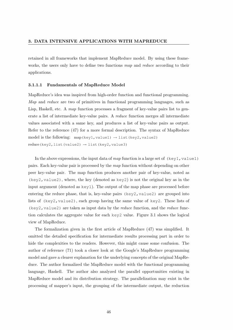
3. DATA INTENSIVE APPLICATIONS WITH MAPREDUCE
retained in all frameworks that implement MapReduce model. By using these frame-
works, the users only have to define two functions map and reduce according to their
applications.
3.1.1.1 Fundamentals of MapReduce Model
MapReduce’s idea was inspired from high-order function and functional programming.
Map and reduce are two of primitives in functional programming languages, such as
Lisp, Haskell, etc. A map function processes a fragment of key-value pairs list to gen-
erate a list of intermediate key-value pairs. A reduce function merges all intermediate
values associated with a same key, and produces a list of key-value pairs as output.
Refer to the reference (47) for a more formal description. The syntax of MapReduce
model is the following: map(key1,value1) → list(key2,value2)
reduce(key2,list(value2) → list(key2,value3)
In the above expressions, the input data of map function is a large set of (key1,value1)
pairs. Each key-value pair is processed by the map function without depending on other
peer key-value pair. The map function produces another pair of key-value, noted as
(key2,value2), where, the key (denoted as key2) is not the original key as in the
input argument (denoted as key1). The output of the map phase are processed before
entering the reduce phase, that is, key-value pairs (key2,value2) are grouped into
lists of (key2,value2), each group having the same value of key2. These lists of
(key2,value2) are taken as input data by the reduce function, and the reduce func-
tion calculates the aggregate value for each key2 value. Figure 3.1 shows the logical
view of MapReduce.
The formalization given in the first article of MapReduce (47) was simplified. It
omitted the detailed specification for intermediate results processing part in order to
hide the complexities to the readers. However, this might cause some confusion. The
author of reference (71) took a closer look at the Google’s MapReduce programming
model and gave a clearer explanation for the underlying concepts of the original MapRe-
duce. The author formalized the MapReduce model with the functional programming
language, Haskell. The author also analyzed the parallel opportunities existing in
MapReduce model and its distribution strategy. The parallelization may exist in the
processing of mapper’s input, the grouping of the intermediate output, the reduction
46

3.1 MapReduce: a New Parallel Computing Model in Cloud Computing
Figure 3.1: Logical view of MapReduce model.
processing over groups and the reduction processing inside each group during the reduce
phase. In the strategy of MapReduce model, network bandwidth is considered as the
scarce resource. This strategy combines parallelization and large data set distributed
storage to avoid saturating the network bandwidth.
Note that the keys used in map phase and reduce phase can be different, i.e. de-
velopers is free to decided which part of data will be keys in these two phases. That
means this data form of key-value pair is very flexible, which is very different from the
intuitive feel. As keys are user-definable, one can ignore the limitation of key-value.
Thus, a whole MapReduce procedure can be informally described as follows:
• Read a lot of data;
• Map: extract useful information from each data item;
• Shuffle and Sort;
• Reduce: aggregate, summarize, filter, or transform;
• Write the results.
47

3. DATA INTENSIVE APPLICATIONS WITH MAPREDUCE
3.1.1.2 Extended MapCombineReduce Model
MapCombineReduce model is an extension of MapReduce model. In this model, an
optional component, namely the combiner, is added to the basic MapReduce model.
This combiner component is proposed and adopted in Hadoop project (11). The in-
termediate output key-value pairs are buffered and periodically flushed onto disk. At
the end of the processing procedure of the mapper, the intermediate key-value pairs
are already available in memory. However, these key-value pairs are not written into a
single file. These key-value pairs are split into R buckets based on the key of each pair.
For the sake of efficiency, we sometimes need to execute a reduce-type operation within
each worker node. Whenever a reduce function is both associative and commutative, it
is possible to ”pre-reduce” each bucket without affecting the final result of the job. Such
a ”pre-reduce” function is referred to as combiner. The optional combiner component
collects the key-value pairs from the memory. Therefore, the key-value pairs produced
by the mappers are processed by the combiner instead of being written into the output
immediately. In such a way, the intermediate output amount is reduced. This makes
sense when the bandwidth is relatively small and the volume of transferred data over
the network is large. Figure 3.2 shows the logical view of MapCombineReduce model.
3.1.2 Two MapReduce Frameworks: GridGain vs Hadoop
Hadoop(11) and GridGain (10) are two different open-source implementations of MapRe-
duce. Hadoop is designed for processing applications. The response time is relatively
long, for instance, from several minutes to several hours. One example of such an
application is the finite element method calculated over a very large mesh. The ap-
plication consists into several steps; each step uses the data generated by the previous
steps. The processing of Hadoop includes transmitting the input data to the comput-
ing nodes. This transfer must be extremely fast to fulfill the users’ need. Hadoop is
an excellent MapReduce supporting tool and a Hadoop cluster gives high throughput
computing. However, it has a high latency since Hadoop is bound with the Hadoop
distributed file system (HDFS). The Hadoop’s MapReduce component operates on the
data or files stored on HDFS, and these operations take a long time to be performed.
For this reason, Hadoop cannot provide a low latency.
48

3.1 MapReduce: a New Parallel Computing Model in Cloud Computing
Figure 3.2: Logical view of MapCombineReduce model.
49
3. DATA INTENSIVE APPLICATIONS WITH MAPREDUCE
However, what we are trying to perform in parallel is a great number of queries on
one large data set. The data set involved is not modified, and the query processing
should be interactive. In fact, low latency is essential for interactive applications. In or-
der to be compatible with the application’s interactive requirements, the response time
is strictly limited, for instance, within five seconds. In contrast to Hadoop, GridGain
is not bound with file system and offers low latency. It is a MapReduce computational
tool. GridGain splits the computing task into small jobs and executes them on the
grid in parallel. During the task execution, GridGain deals with the low-level issues,
such as nodes discovery, communication, jobs collision resolution, load balancing, etc.
Being compared with Hadoop, GridGain is more flexible. Instead of accessing data
stored on distributed file system, GridGain can process data stored in any file system
or database. In addition, GridGain has some other advantages. For instance, it does
not need application deployment and can be easily integrated with other data grid
products. In particular, it allows programmers to write their programs in pure Java
language.
3.1.3 Communication Cost Analysis of MapReduce
In parallel programming, a computation is partitioned into several tasks, which are allo-
cated to different computing nodes. The communication cost issues must be considered
since the data transmission between the computing nodes represents a non-negligible
part. The communication cost is directly linked with the degree of parallelism. If the
tasks are partitioned with a high degree of parallelism, the communication cost will be
large. On the other hand, if the degree of parallelism is small, the communication cost
will be limited.
In MapReduce parallel model, the communication cost exists in several phases. For
the basic MapReduce model, without a combiner component, the communication cost
consists in three distinct phases. The first phase is the launching phase, during which
all the tasks are sent to the mappers. The second phase, located between mappers and
reducers, consists in sending the output from mappers to reducers. The third phase
is the final phase, which produces the results and where the outputs of the reducers
are sent back. For the extended MapCombineReduce model, the communication con-
sists in four phases. The first phase is still the launching phase. The second phase,
located between mappers and combiners, consists to send the intermediate results from
50
3.1 MapReduce: a New Parallel Computing Model in Cloud Computing
mappers to combiners located on the same node. The third phase, located between
the combiner and the reducer, consists to send the output of combiners to reducers.
The fourth phase is the final phase, which produces the results. The size of the output
data exchanged between the components strongly impacts the communication cost. In
reference (62), the author described an analysis for the communication cost in a par-
allel environment, depending on the amount of data exchanged between the processes.
Basing on their work we analyzed the case of MapReduce, we summarized the following
factors influencing the communication cost.
(i) The first one is the amount of intermediate data to be transferred, from the mappers
to the reducers (case without a combiner component) or from the combiners to
the reducers (case of a combiner component).
(ii) The second factor is the physical locations of the mappers, the combiners and the
reducers. If two communicating components are on the same node, the communi-
cation cost is low; otherwise the cost is high. If two communicating components
are located on two geographically distant nodes, the communication cost could
be extremely high!
(iii) The third factor to be considered is the number of mappers, combiners and reduc-
ers respectively. Usually, the user defines the number of mappers according to the
scale of the problem to be solved and the computing capacity of the hardware.
The number of combiners is usually equal to the number of nodes participating
to the calculation, as are devoted to collect local intermediate result of a node.
Whether or not the number of reducers can is user-definable depends on the de-
sign of the implemented MapReduce framework. For example Hadoop allows the
user to specify the number of reducers. Opposite, GridGain fixes the value of the
number of reducers to one.
(iv) The fourth factor is the existence of a direct physical connection between two com-
municating components. A direct physical connection between two components
means that two nodes respectively holding the two components are physically
connected to each other.
(v) The last factor is the contention over the communicating path. When two or more
communications are executed at the same time, the contention of the bandwidth
51
3. DATA INTENSIVE APPLICATIONS WITH MAPREDUCE
will appear. A possible scenario of this contention with MapReduce model could
be described as follows. The mappers on various nodes are started at almost the
same time. Since the nodes in a cluster are usually of identical type, they almost
have the same capability. As a consequence, the mappers complete their work on
each node at the same time. The outputs of these mappers are then sent to the
reducers. In this scenario, the contention of the communicating path is caused
by the transmission requests arriving almost simultaneously.
Since the actions of transferring the data from the master node to the worker nodes
are generally much more costly than the actions of transferring the mappers from the
master to the workers, we usually transfer the mapper job code towards the location
of data. Thus, the geographical locations of the data have a strong impact on the
efficiency.
3.1.4 MapReduce Applications
MapReduce was initially proposed to support the search operation among a large
amount of web pages. It is naturally capable of handling large-scale unstructured
data, i.e. data-intensive text processing. An example of data-intensive text-processing
is website log analysis. Website uses log to record users’ behaviours or activities, which
generates a large volume of data. Analysing this information allows providing additional
services. For example, with log analysing, an on-line selling website may recommend
the new products to a client which is relative to the product that he or she already
purchased.
The large-scale structured data analysis applications, such as OLAP query pro-
cessing can benefit from MapReduce. For utilizing MapReduce to serve data analysis
applications, there still exist some challenges. Firstly, MapReduce does not directly sup-
port relational algebraic operators and query optimization. Secondly, being compared
with the high-level declarative data query and manipulation language SQL, MapRe-
duce is only a low-level procedural programming paradigm. In order to benefit from
MapReduce, a combination of MapReduce and SQL is expected for data intensive ap-
plications in a near future. The combination between MapReduce and SQL consists
in realizing and optimizing each relational algebra operator. Some SQL queries can be
directly and naturally realized using MapReduce, for example, such as select queries.
52
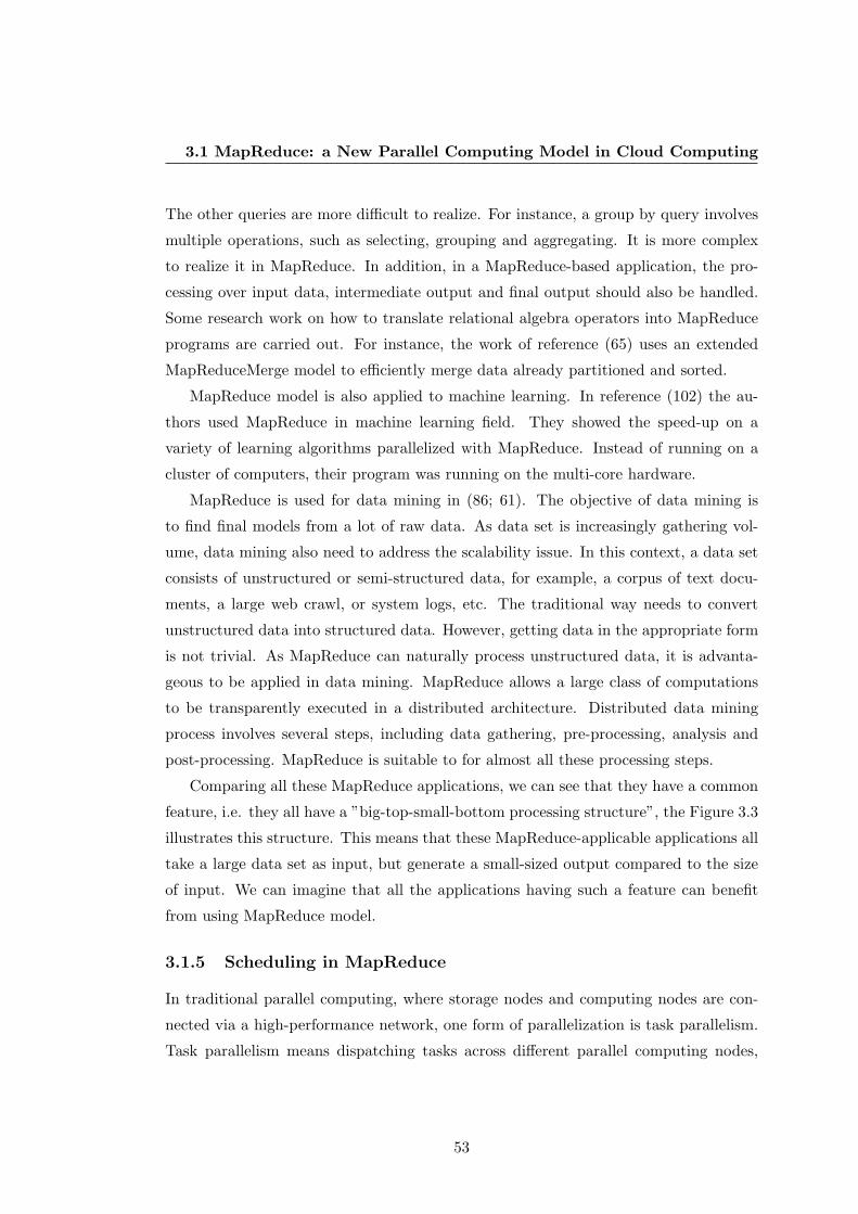
3.1 MapReduce: a New Parallel Computing Model in Cloud Computing
The other queries are more difficult to realize. For instance, a group by query involves
multiple operations, such as selecting, grouping and aggregating. It is more complex
to realize it in MapReduce. In addition, in a MapReduce-based application, the pro-
cessing over input data, intermediate output and final output should also be handled.
Some research work on how to translate relational algebra operators into MapReduce
programs are carried out. For instance, the work of reference (65) uses an extended
MapReduceMerge model to efficiently merge data already partitioned and sorted.
MapReduce model is also applied to machine learning. In reference (102) the au-
thors used MapReduce in machine learning field. They showed the speed-up on a
variety of learning algorithms parallelized with MapReduce. Instead of running on a
cluster of computers, their program was running on the multi-core hardware.
MapReduce is used for data mining in (86; 61). The objective of data mining is
to find final models from a lot of raw data. As data set is increasingly gathering vol-
ume, data mining also need to address the scalability issue. In this context, a data set
consists of unstructured or semi-structured data, for example, a corpus of text docu-
ments, a large web crawl, or system logs, etc. The traditional way needs to convert
unstructured data into structured data. However, getting data in the appropriate form
is not trivial. As MapReduce can naturally process unstructured data, it is advanta-
geous to be applied in data mining. MapReduce allows a large class of computations
to be transparently executed in a distributed architecture. Distributed data mining
process involves several steps, including data gathering, pre-processing, analysis and
post-processing. MapReduce is suitable to for almost all these processing steps.
Comparing all these MapReduce applications, we can see that they have a common
feature, i.e. they all have a ”big-top-small-bottom processing structure”, the Figure 3.3
illustrates this structure. This means that these MapReduce-applicable applications all
take a large data set as input, but generate a small-sized output compared to the size
of input. We can imagine that all the applications having such a feature can benefit
from using MapReduce model.
3.1.5 Scheduling in MapReduce
In traditional parallel computing, where storage nodes and computing nodes are con-
nected via a high-performance network, one form of parallelization is task parallelism.
Task parallelism means dispatching tasks across different parallel computing nodes,
53
3. DATA INTENSIVE APPLICATIONS WITH MAPREDUCE
Figure 3.3: Big-top-small-bottom processing structure of MapReduce suitable applica-tions
which involves moving data to nodes where the computations occur. The task par-
allelism, characterized by moving data, is not suitable for data-intensive applications.
The workload of data-intensive applications will suffer from network congestion when
moving large amount of data across network, which causes a bottleneck of system. An-
other form of parallelism is data parallelism. Data parallelism focuses on distributing
data across different computing nodes. In a system of multiple computing nodes, Data
Parallelism is achieved when each node performs a task over a piece of distributed data.
MapReduce follows the same idea as Data Parallelism, moving programs instead of
moving data. In a distributed architecture running MapReduce, computing nodes and
storage nodes co-locate on same machines. Computation is sent to a node having or
close to the received data and execute on it. MapReduce assumes a distributed archi-
tecture being composed of one master node and many worker nodes. For a MapReduce
procedure, a common scheduling is described as following.
1. The input is split into M blocks, each block is processed by a mapper ;
2. Mappers are assigned and started on free worker nodes;
3. Each mapper produces R local files containing intermediate data;
54
3.1 MapReduce: a New Parallel Computing Model in Cloud Computing
4. Reducers are assigned and started when all mappers were finished, processing
intermediate data read from mapper workers.
When the master node assigns mapper to a free worker node, it takes into account
the locality of data to the worker node. The worker nodes closest to or having the
needed data are chosen. The output of each mapper is partitioned into R local files
containing intermediate key-value pairs. A shuffle over all intermediate key-value pairs
is automatically run after all the intermediate outputs are available, before starting the
reducer. When the master node assigns reducer to a free worker node, the worker node
reads the intermediate key-value pairs from remote worker nodes where were running
mappers. Worker node then sorts and applies reduce logic which produces the final
output.
Comparing with traditional scheduling used in parallel computing, the job schedul-
ing within a MapReduce processing need to mainly consider two additional aspects(79):
• the need for data locality (running computing where the data is);
• the dependence between mapper and reducer.
In Hadoop, one of the implemented MapReduce frameworks, a speculative task
execution is realized. This speculative execution is aiming to address the straggler
nodes. As a barrier exists between map phase and reduce phase, the reducer cannot
be started until all mappers finished. Thus, the speed of MapReduce fully depends
on the slowest node running mapper, which is called straggler node. With speculative
execution, an identical mapper of straggler node is executed on a different worker
node, and the framework simply uses the result of the first task attempt to finish. Both
mappers and reducers can be speculatively executed. Hadoop uses a slots model for
task scheduling over one worker node. Each worker node has a fixed number of mapper
slots and reducer slots. When a slot becomes free, the scheduler will scan through tasks
ordered by priority and submit time to find a task to fill the slot. The scheduler also
considers the data locality when it assigns a task of mapper1
Another framework implementing MapReduce model, GridGain, has a limitation
over the reducer number. The number of reducer is fixed as one, which means only one
1Scheduler chooses the node holding the needed data block, if it is possible. Otherwise, schedulerchooses a node within a same rack as the neede data blocks holding node.
55

3. DATA INTENSIVE APPLICATIONS WITH MAPREDUCE
reducer is run when all mappers were finished their computations. The reducer is run
on the master node. In such a context, the scheduling is simplified. GridGain provides
several policies for scheduling mappers. Especially, GridGain provides a Data affinity
policy for dispatching jobs over nodes. If a previous mapper using a data block, saying
A, is assigned to a worker node, noted as a, then the next task using the same data
block A will still be assigned to the worker node a.
When there are multiple jobs to be executed, Hadoop schedules these jobs follow-
ing the FIFO policy. The reference (57) considers a multi-user environment. Their
work designed and implemented a fair scheduler for Hadoop. The fair scheduler gives
each user an illusion of owning a private Hadoop cluster, letting user to start jobs
within seconds and run interactive queries, while utilizing an underlying shared cluster
efficiently.
Some jobs need not only one time MapReduce procedure, but multiple times MapRe-
duce procedures. In this case, one MapReduce job cannot accomplish the whole job,
and then a chain of MapReduce can be used to realize such large jobs, i.e. multi-stage
MapReduce.
3.1.6 Efficiency Issues of MapReduce
The efficiency of MapReduce is a matter of debate for data analysis. The fundamental
reason is that MapReduce is not initially designed for data analysis system over struc-
tured data. The typical calculations involved in MapReduce are scanning over a lot of
unstructured data, like web page. In contrast, the data analysis applications typically
accesses structured data. Comparing to the brute-force scan over unstructured data,
the measures for accelerating query over structured data are abundant, such index,
materialized view, column-oriented store. However, people argued that the lack of data
structure is not a limitation, because MapReduce skip the data-loading phase, and im-
mediately read data off of the file system and answer query on the fly, without any kind
of loading stage. In the traditional data analysis, the data-loading phase is to load data
using a pre-defined schema. Still, the optimization, like index and materialized view
can unquestionably improve the performance. Especially, these optimization only need
to be done one-time, and are reusable for all processing of query. In fact, data loading
phase could also be exploited in MapReduce. For example, data compression can be
56

3.2 Distributed Data Storage Underlying MapReduce
done in data loading phase, which can accelerate brute-force scan. Without data load-
ing, MapReduce needs to parse data each time it accesses data, instead of parsing data
only once as load time. The efficiency of MapReduce depends on the applications in
which it is used. For complex analysis of unstructured data, where brute-force scan is
the right strategy, MapReduce is suitable. On the contrary, for business-oriented data
analysis market, special MapReduce-based algorithms need to be created to obtain high
efficiency.
3.1.7 MapReduce on Different Hardware
MapReduce is typically running across multiple machines connected in a shared-nothing
fashion. People tried to run MapReduce over other different hardware. MapReduce can
be run on shared-memory, multicore and multi-processor systems. In the reference (90),
the author realized a specific implementation of MapReduce for shared-memory system.
This shared-memory MapReduce automatically manages thread creation, dynamic task
scheduling, and fault tolerance across processor nodes. Another specific implementation
of MapReduce running on Cell BE architecture is introduced in (46). MapReduce can
also run on graphics processors (GPUs). A GPU specialized MapReduce framework,
Mars, was proposed in (63).
3.2 Distributed Data Storage Underlying MapReduce
The data-driven nature of MapReduce requires a specific underlying data storage sup-
port. High-Performance Computing’s traditional separating storage component from
computations is not suitable for processing large size data set. MapReduce abandons
the approach of separating computation and storage. In the runtime, MapReduce needs
to either access data on local disk, or access data stored closely to the computing node.
3.2.1 Google File System
Google uses a distributed Google File System (GFS) (57; 87) to support MapRe-
duce computations. Hadoop provides an open-source implementation of GFS, which
is named Hadoop Distributed File System (HDFS) (12). In Google, MapReduce is
implemented on top of GFS and running over within clusters. The basic idea of such
GFS is to divide a large data set into chunks, then replicate each chunk across different
57
3. DATA INTENSIVE APPLICATIONS WITH MAPREDUCE
nodes. The chunk size is much larger than in the traditional file system. The default
chunk size is 64M in GFS and HDFS.
The architecture of GFS follows master-slave model. The master node is responsible
of maintaining file namespace, managing and monitoring the cluster. Slave nodes man-
age their actual chunks. Data chunks are replicated across slave nodes, with 3 replicas
by default. When an application wants to read a file, it needs to consult the metadata
information about chunks by contacting the master node to know on which slave nodes
the required chunk is stored. After that, application contacts the specific slave nodes
to access data. The size of chunk is a crucial factor influencing the amount of data
that the master node needs to handle. The default chunk size considers a trade-off
between trying to limit resource usage and master interaction times on the one hand
and accepting an increased degree of internal fragmentation on the other hand.
GFS is different from the general applicative File System, such as NFS or AFS.
GFS assumes that data is updated in an append-only fashion(36), and data access
is mainly long streaming reads. GFS is optimized for workload characterized of the
above-mentioned features. The following summarizes GFS’s characteristics:
• GFS is optimized for the usage of large files, where the space efficiency is not very
important;
• GFS files are commonly modified by being appended data;
• Modifying at file’s arbitrary offset is infrequent operation;
• GFS is optimized of large streaming reads;
• GFS supports great throughput, but has long latency;
• Client’s caching techniques are considered as ineffective.
A weakness of GFS master-slave is the single master node. The master node plays
a crucial role in GFS. It does not only manage metadata, but also maintains the file
namespace. In order to avoid the master node becoming a bottleneck, the master
has been implemented using multi-threading and fine-grained locking. Additionally, in
order to alleviate the workload of master node, master node is designed to only provide
metadata to locate chunks, and it does not participate the following data accessing.
58

3.2 Distributed Data Storage Underlying MapReduce
Rick of single point of failure is another weakness of GFS. Once the master node crushes,
the whole file system will stop working. For handling master’s crush, a shadow masters
design is adopted. The shadow master holds a copy of the newest operation log. When
master node crushes, the shadow master provides read-only access of metadata.
3.2.2 Distributed Cache Memory
The combination of MapReduce and GFS guarantee high throughput since GFS is
optimized for sequential reads and appends on large files. However, such a combination
has a high latency. GFS-based MapReduce heavily use disk, in order to alleviate
the affect brought by failures. However, this produces a large amount of disk I/O
operations. The latency for disk access is much higher than that of memory access. In
GFS-based MapReduce, memory was not fully utilized (110). In the GFS open-source
implementation, HDFS, reading data also suffers from high latency. Reading a random
chunk in HDFS involves multiple operations. For instance, it needs communicating
with master to get the data chunk location. If data chunk is not located on the node
where read operation occurs, then that also requires performing data transfer. Each of
these operations leads to higher latency(76).
The authors of reference (110) argued that small-scale MapReduce clusters, which
have no more than dozen of machines, are very common in most companies and lab-
oratories. Node failures are infrequent in clusters of such size. So it is possible to
construct a more efficient MapReduce framework for small-scale heterogeneous clus-
ters using distributed memory. The author of the reference (76) also proposed the
idea of utilizing distributed memory. Both of these works have chosen the open-source
distributed in-memory object caching system, memcached to provide an in-memory
storage to Hadoop.
In the work of (76), the whole data set, in form of key-value pair, is loaded into
memcached from HDFS. Once the whole data set is in memcached, the subsequent
MapReduce programs access data with the client API of memcached. Each mapper
or reducer maintains connections to the memcached servers. All requests happen in
parallel and are distributed across all memcached servers.
In the work of (110), only the output of mappers is loaded into memcached. The
cached mapper’s output is attached with a key. Such a key is made up of a mapper id
59

3. DATA INTENSIVE APPLICATIONS WITH MAPREDUCE
and its target reducer id. Once a reducer is started, it checks whether the outputs for
it are in memcached. If that is true, then it gets them from memcached server.
3.2.3 Manual Support of MapReduce Data Accessing
If a MapReduce framework without being attached with a distributed file system is
used, then data locating needs to be taken charge of developers. GridGain is such a pure
MapReduce computing framework, and it is not attached with any distributed storage
system. Although this forces developers to do the low-level work of data locating, to
some extent, this provides some flexibility. Data accessing does not need to consult the
file namespace any more; the other data forms than files can also be the representation
of distributed stored data, e.g. data can be stored in database on each computing node.
GridGain’s MapReduce is composed of one master node and multiple worker nodes.
GridGain provides useful mecanism for users to add user properties, which is visible
to master. Master node can identify worker nodes from the added properties. The
additional properties defined by user can be used for different purposes, such as, logical
name of node, role name of node etc. As we adopted GridGain as the MapReduce
framework, we give an example coming from our work. In this work, we added to
each worker node a property representing the identifier of data fragment stored in the
current worker node.
In the manual approach, a data pre-processing phase is indispensable. During this
phase, data set is divided into blocks, and distributed/replicated across different worker
nodes. Using the method mentioned above, a user-defined property representing data
fragment identifier is added to each worker node. As being visible to master node,
this user-defined property is used for locating data chunks. An illustration is given
in the Figure 3.4. As this manual approach decouples underlying storage from the
computations, it provides the possibility to choose various underlying data storages.
Mappers can access third-part data source. As developer can personally control data
locating, then data transfer between worker nodes is less frequent than in the GFS-
based MapReduce system. More importantly, the optimization over data accessing can
be performed without being limited by a particular file system.
60

3.2 Distributed Data Storage Underlying MapReduce
Figure 3.4: Manual data locating based on GridGain: circles represent mappers to bescheduled. The capital letter contained in each circle represents the data block to beprocessed by a specific mapper. Each worker has a user-defined property reflecting thecontained data, which is visible for master node. By identifying the values of this property,the master node can locate data blocks needed by each mapper.
61

3. DATA INTENSIVE APPLICATIONS WITH MAPREDUCE
3.3 Data Management in Cloud
Cloud computing is an internet-based computing system, which integrates resources
ranging from computer processing, storage and software available across network. Ama-
zon, Google, Microsoft all put forward the concept of Cloud Computing. So far, there
already exist multiple commercial products. Amazon Simple Storage Service (Amazon
S3) (2) and Amazon Elastic Compute Cloud (Amazon EC2) (1) provide small-scale en-
terprises with computing and storage services. Google App Engine (7) allows running
the third-part parallel programs on its cloud. Microsoft’s Windows Azure Platform
(22) provides a Windows-based environment for running applications and storing data
on servers in data centers. More details can be find in reference (109), an article on
state-of-the-art of cloud computing.
Data storage in the new cloud platform is different than before. Replicated and
distributed are two of main characteristics of data stored in cloud. Data is automati-
cally replicated without the interference of users. Data availability and durability are
achieved through replication. Large cloud provider may have data centers spread across
the world.
3.3.1 Transactional Data Management
Data stored in fashion of cloud—replicated and distributed—is considered to be un-
suitable for transactional data management applications(25). In traditional data man-
agement system, a transaction should support ACID, which means all computations
contained in a transaction should be Atomicity, Consistency, Isolation and Durability.
Such a guarantee is important for write-intensive applications. However, the ACID
guarantee is difficult to be achieved on replicated and distributed data storage. Among
full-fulfilled database products, shared-nothing architecture is not commonly used for
transactional data management. Realizing a transaction on a shared-nothing architec-
ture involves complex distributed locking which is non-trivial work. The advantage of
scalability coming with shared-nothing architecture is not an urgent need for transac-
tional data management.
62

3.4 Large-scale Data Analysis Based on MapReduce
3.3.2 Analytical Data Management
Analytical data management applications are commonly used in business planning
problem solving, and decision support. Data involved by analytical data management
is often historical data. Historical data usually has large size, and is read-mostly (or
read-only), and occasionally batch updated. Analytical data management applications
can benefit from cloud data storage. Analytical data management applications are
argued to be well-suited to run in a Cloud environment (25), since analytical data
management matches well with shared-nothing architecture, and ACID guarantees are
not needed for it.
3.3.3 BigTable: Structured Data Storage in Cloud
BigTable(37) is a distributed structured data storage system. Hadoop provided HBase
(13), an open-source implementation of BigTable. BigTable provided a flexible, high-
performance solution for various Google applications with varied demands. MapReduce
is one of applications using BigTable. Different applications in Google could be latency-
sensitive or they need high-throughputs. A BigTable is a sparse, distributed, persistent
multidimensional sorted map, indexed by a row key, column key and a time-stamp.
Thus, it shares characteristics of both row-oriented storage and column-oriented stor-
age. GFS is used to store log and data files in BigTable. The cluster management takes
charge of job scheduling, resource managing on shared machines, dealing with machine
failures, as well as monitoring machine status. BigTable API provides functions for
creating and deleting tables and column families1, changing cluster, table, and column
family metadata.
3.4 Large-scale Data Analysis Based on MapReduce
Data analysis applications or OLAP applications are encountering scalability issue.
Facing more and more generated data, OLAP software should be able to handle data
sets much larger than ever. MapReduce naturally has good scalability, and people
argued that MapReduce approach is suitable for data analysis workload. The key is
to choose an appropriate implementation strategy for the given data analysis applica-
tion. For choosing an appropriate implementation strategy to process an data analysis
1Column family refers to several column keys being grouped into sets.
63

3. DATA INTENSIVE APPLICATIONS WITH MAPREDUCE
query, two types of questions need to be answered. The first question is about the data
placement. This short term includes several sub-questions: What is the most suitable
data-partitioning scheme? To which degree we will partition the data set? What is the
best data placement strategy of data partitions? The second question is how to effi-
ciently perform the query over the distributed data partitions? In a MapReduce based
system, the query’s calculation is transformed to another problem, how to implement
the query’s processing with MapReduce? To answer to these questions, the specific
analysis addressing various queries needs to be undertaken.
3.4.1 MapReduce-based Data Query Languages
Hadoop’s rudimentary support for MapReduce, promoted the development of MapReduce-
based high-level data query languages. A data query language PigLatin (40), was orig-
inally designed by Yahoo, and later became an open-source project. It is designed as
a bridge between low-level, procedural style of MapReduce and high-level declarative
style of SQL. It is capable of handling structured and semi-structured data. Program
written in PigLatin is translated into physical plans being composed of MapReduce
procedures during compiling. The generated physical plans are then executed over
Hadoop.
Similarly, another open-source project, Hive (14) of Facebook, is a Data Warehouse
infrastructure built on top of Hadoop. It allows aggregating data, processing ad hoc
query, and analysing data stored in Hadoop files. HiveQL is an SQL-like language,
which allows querying over large data set stored as HDFS files.
Microsoft developed MapReduce-based declarative and extensible scripting lan-
guage, SCOPE (Structured Computations Optimized for Parallel Execution) (91),
targeted for massive data analysis. This language is high-level declarative, and the
compiler together with optimizer can improve SCOPE scripts through compiling and
optimizing. SCOPE is extensible. Users are allowed to create customized extractors,
processors, aggregators and combiners by the extending built-in C# components.
3.4.2 Data Analysis Applications Based on MapReduce
An attempt of MapReduce-based OLAP system was described in (39). The following
description of their work lays out a clear example of doing data analysis with MapRe-
duce. The data set used in their work is a data cube. In particular, the data cube was
64

3.4 Large-scale Data Analysis Based on MapReduce
coming from a web log, which is employed to analyse the web search activities. More
specifically, the data cube is composed of 2 dimensions (keyword k and time t) and 2
measures (page count: pageCount and advertisement count: adCount). During data
partitioning, the data cube is divided over dimensions of keyword and time. The cells
having the same value of k and t are put into one block. Similar to the MOLAP, the
hierarchy concept is applied over the data cube in their work. These different hierar-
chy levels in time dimension allow partitioning data cube with different granularities.
Support of dynamic data partitioning granularity is a unique feature of this work. As
queries processed in their work are correlated, the results generated for one query can
serve as the input for another query. However, the granularity of the second query is not
necessarily the same as in the first query, and then the change of granularity is needed.
The MapReduce-based query processing concerns two groups of nodes: nodes running
mappers, and nodes running reducers. The group of nodes is done at the beginning of
query processing. Mapper fetches part of data set and generates key-value pairs from
individual record. The key field is related to different granularities, which in turn de-
pends on the query, and it can be computed using the given algorithms. The value field
is the exact copy of the original data record. These key-value pairs are shuffled, and
dispatched to reducers. The pairs with the same key go to the same reducer. Reducer
performs an external sorting to group pairs with the same value. Then it produces an
aggregated result for each group.
Regarding the commercial software, MapReduce was integrated into some commer-
cial software products. Greenplum is a commercial MapReduce database, which enables
programmers to perform data analysis on petabyte-scale data sets inside and outside
of it (8). Aster Data Systems, a database software company has recently announced
the integration of MapReduce with SQL. Aster’s nCluster allows implementing flexible
MapReduce functions for parallel data analysis and transformation inside the database
(3).
3.4.3 Shared-Nothing Parallel Databases vs MapReduce
Although being able to run on different hardware, MapReduce is typically running on a
shared-nothing architecture where computing nodes are connected by network without
memory or disk sharing among each other. Many parallel databases adopted shared-
65
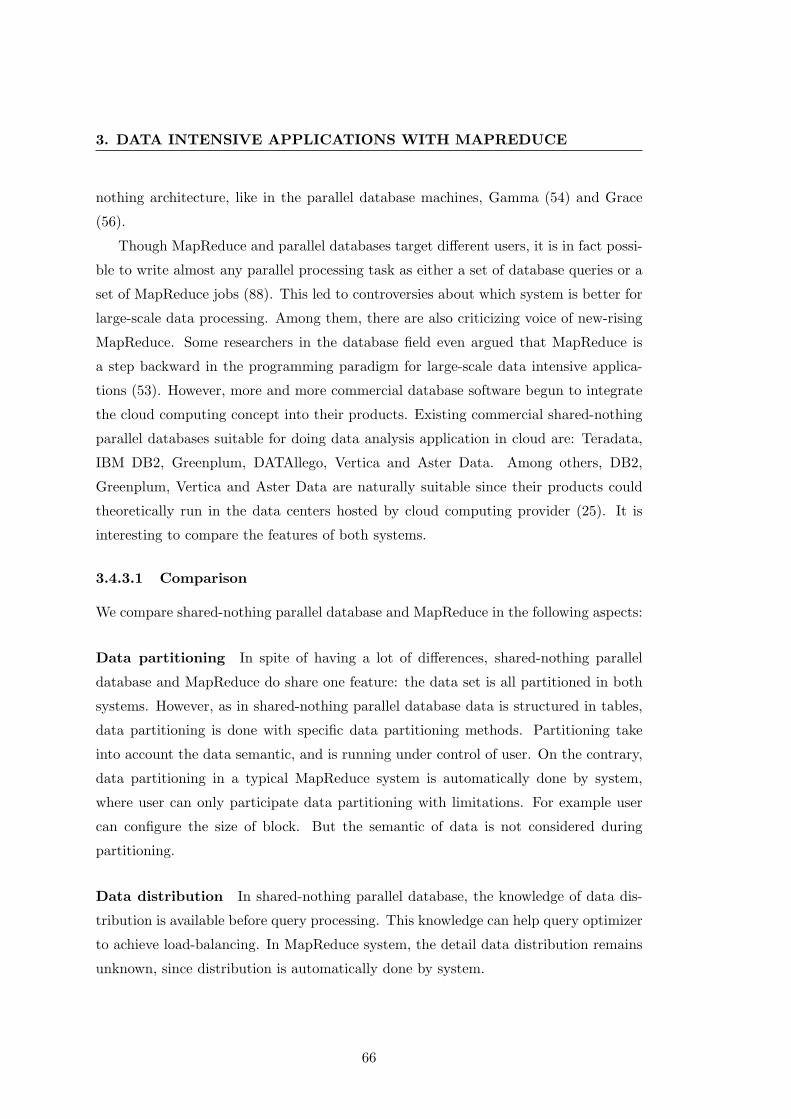
3. DATA INTENSIVE APPLICATIONS WITH MAPREDUCE
nothing architecture, like in the parallel database machines, Gamma (54) and Grace
(56).
Though MapReduce and parallel databases target different users, it is in fact possi-
ble to write almost any parallel processing task as either a set of database queries or a
set of MapReduce jobs (88). This led to controversies about which system is better for
large-scale data processing. Among them, there are also criticizing voice of new-rising
MapReduce. Some researchers in the database field even argued that MapReduce is
a step backward in the programming paradigm for large-scale data intensive applica-
tions (53). However, more and more commercial database software begun to integrate
the cloud computing concept into their products. Existing commercial shared-nothing
parallel databases suitable for doing data analysis application in cloud are: Teradata,
IBM DB2, Greenplum, DATAllego, Vertica and Aster Data. Among others, DB2,
Greenplum, Vertica and Aster Data are naturally suitable since their products could
theoretically run in the data centers hosted by cloud computing provider (25). It is
interesting to compare the features of both systems.
3.4.3.1 Comparison
We compare shared-nothing parallel database and MapReduce in the following aspects:
Data partitioning In spite of having a lot of differences, shared-nothing parallel
database and MapReduce do share one feature: the data set is all partitioned in both
systems. However, as in shared-nothing parallel database data is structured in tables,
data partitioning is done with specific data partitioning methods. Partitioning take
into account the data semantic, and is running under control of user. On the contrary,
data partitioning in a typical MapReduce system is automatically done by system,
where user can only participate data partitioning with limitations. For example user
can configure the size of block. But the semantic of data is not considered during
partitioning.
Data distribution In shared-nothing parallel database, the knowledge of data dis-
tribution is available before query processing. This knowledge can help query optimizer
to achieve load-balancing. In MapReduce system, the detail data distribution remains
unknown, since distribution is automatically done by system.
66

3.4 Large-scale Data Analysis Based on MapReduce
Support for schema Shared-nothing parallel databases require data conform to a
well-defined schema; data is structured with rows and columns. In contrast, MapReduce
permits data to be any arbitrary format. MapReduce programmer is free of schema,
and data can even have no structure at all.
Programming model Like other DBMSs, shared-nothing parallel database supports
a high-level declarative programming language, i.e. SQL, which is known for and largely
accepted by both professional and non-professional users. With SQL, users only need
to declare what they want to do, but do not need to provide a specific algorithms to
realize it. However, in MapReduce system, developers must provide an algorithm in
order to realize the query processing.
Flexibility SQL is routinely criticized for its insufficient expressive power. In order
to mitigate flexibility, shared-nothing parallel databases allow user-defined functions.
MapReduce has good flexibility by allowing developers to realize all calculations in the
query processing.
Fault tolerance Both parallel database and MapReduce use replication to deal with
disk failures. However, parallelism databases cannot handle node failures, since they do
not save intermediate results, once a node fails, the whole query processing should be
restarted. MapReduce is able to handle node failure during the execution of MapReduce
computation. The intermediate results (from mappers) are stored before launching
reducers in order to avoid starting the processing from zero in case of node failure.
Indexing Parallel databases have many indexing techniques, such hash or B-tree, to
accelerate data access. MapReduce does not have built-in indexes.
Support for Transactions The support for transactions requires the processing
to respect ACID. Shared-nothing parallel databases support transaction, since it can
easily respect ACID. But it is difficult for MapReduce to respect such a principle. Note
that, in large-scale data analysis, the ACID is not really necessary.
67

3. DATA INTENSIVE APPLICATIONS WITH MAPREDUCE
Scalability Shared-nothing parallel database can scale well to tens of nodes, but
difficult to go any further. MapReduce has very good scalability, which is proved by
Google’s use. It can scale to thousands nodes.
Adaptability over heterogeneous environment As shared-nothing parallel database
is designed to run in homogeneous environment, it is not suited to run in heterogeneous
environment. MapReduce is able to run in heterogeneous environment.
Execution strategy MapReduce has two phases, map phase and reduce phase. Re-
ducers need to pull each of its input data from the nodes where mappers were run.
Shared-nothing parallel databases uses a push approach to transfer data instead of
pull.
Table 3.1 summarizes the differences between parallel database and MapReduce
with short descriptions.
Parallelism database MapReduceData partitioning Use specific methods Done automatically
consider data semantic do not consider data semanticData distribution Known for developers UnknownSchema support Yes NoProgramming model Declarative Direct realizeFlexibility Not good GoodFault tolerance Handle disk failures Handle disk and node failuresIndexing Support Have no built-in indexTransaction support Yes NoScalability Not good GoodHeterogeneous Unsuitable SuitableenvironmentExecution strategy Push mode Pull mode
Table 3.1: Differences between parallel database and MapReduce
3.4.3.2 Hybrid Solution
MapReduce-like software, and shared-nothing parallel databases have their own advan-
tages and disadvantages. People look for a hybrid solution that combines the fault
tolerance, heterogeneous cluster, and ease of scaling of MapReduce and the efficiency,
performance, and tool plug-ability of shared-nothing parallel database.
68

3.5 Related Parallel Computing Frameworks
HadoopDB (27) is one of the attempts for constructing such a hybrid system. It
combines parallel databases and MapReduce to exploit both the high performance
from the parallel database and scalability from MapReduce. The basic idea behind
HadoopDB is to use MapReduce as the communication layer above multiple nodes
running single-node DBMS instances. Queries are expressed in SQL, translated into
MapReduce by extending existing tools, and as much work as possible is pushed into
the higher performing single node databases. In the experiments their work, they tested
several frequently used SQL-queries, such as select query, join query, simple group-by
query, etc. over one or more of the three relations.
Another way to realize such a hybrid solution is to integrate parallel database
optimization as a part of calculations running with MapReduce. Since MapReduce
does not give any limitations over the implementations, such a hybrid solution is totally
feasible. Our work’s approach also belongs to the hybrid solution.
3.5 Related Parallel Computing Frameworks
Like MapReduce, Dryad system (66) also provides an abstraction that hides system-
level details from developers. The system-level details include fine-grain concurrency
control, resource allocation, scheduling, component failures etc. Dryad provides an
appropriate abstraction level for developers to write the scalable applications. In Dryad,
a job is expressed as a directed acyclic graph where each vertex represents developer-
specified subroutines and edges represent data channels that caption dependencies.
Dryad allows developers to write sub-routines as sequential programs. Such a logical
computation graph is then mapped onto physical resources by the framework.
DryadLINQ (108) is high-level language programming environment based on Dryad.
DryadLINQ combines Dryad and .NET Language Integrated Query (LINQ). LINQ
allows developers to write large-scale data parallel application in a SQL-like query
language. DryadLINQ translates LINQ programs into distributed Dryad computations
that are run within Dryad system.
An academic research project, YvetteML (YML) (49), is a framework aiming to
exploit distributed computing architectures and peer-to-peer systems. YML, together
with various low-level middlewares addressing different distributed architectures, pro-
vides users with an easy way to utilize these distributed architectures. The provided
69

3. DATA INTENSIVE APPLICATIONS WITH MAPREDUCE
workflow language Yvette allows describing an application with a directed acyclic graph,
with the vertex representing component1 and edges represents the timing relationship
between components when being executed. Developers need to write components and
the Yvette program when realizing a distributed application over YML framework.
3.6 Summary
In this chapter, we first introduced the basic idea and related issues of MapReduce
model and its extended model, MapCombineReduce. Two implementation frameworks
of MapReduce, Hadoop and GridGain were presented. They have different latency.
Hadoop has high latency, while GridGain has low latency. Under the interactive re-
sponse time requirement, GridGain is a suitable choice for our work. MapReduce
model hides the underlying communication details. We specially analysed the commu-
nication cost of MapReduce procedure, and discussed the main factors that influence
the communication cost. We then discussed the job-scheduling issues in MapReduce. In
MapReduce job-scheduling, two more things need to be considered than in other cases,
data locality and dependence between mapper and reducer. Our discussion also involves
MapReduce efficiency and its application on different hardware. Secondly, we described
the distributed data storage underlying MapReduce, including distributed filesystems,
like GFS and its open source implementation—HDFS, and efficient enhanced storage
system basing on cache mechanism. Another approach is manual support of MapRe-
duce data access adopted in our work. The third topic addressed in this chapter is
data management in cloud. The suitability of being processed with MapReduce was
discussed for transactional data management and analytical data management. The
latter was thought to be able to benefit from MapReduce model. Relying on this, we
further addressed large-scale data analysis based on MapReduce. We presented the
MapReduce-based data query languages and data analysis related work with MapRe-
duce. As shared-nothing parallel database and MapReduce system use similar hard-
ware, we specially did the comparison between them, followed by presenting the related
work of a hybrid solution of combining these two into one system. Finally, we intro-
duced related parallel computing frameworks.
1A component is a pre-compiled executable which realizes the user-defined computations
70
4
Multidimensional Data
Aggregation Using MapReduce
In this chapter, we will present the MapReduce-base multidimensional data aggrega-
tion. We will first describe the background of our work, as well as the organization
of data used in our work. Then we will introduce Multiple Group-by query, which is
also the calculation that we will parallelize relying on MapReduce. We will give two
implementations of Multiple Group-by query, one is based on MapReduce, and the
other is based on MapCombineReduce. The job definitions for each implementation
will be specifically described. We also will present the performance measurement and
execution time analysis.
4.1 Background of This Work
In the last ten years, more and more BI products use data visualization technique to
support decision-making. Data visualization means using computer-supported, interac-
tive, visual representation of abstract data to reinforce cognition, hypothesis building
and reasoning. Facing to the growing volume of historical data, data visualization
is becoming an indispensable tool helping decision-maker to extract useful knowledge
from large amount of data. Typically, the abstract data is represented as dashboards,
charts, maps, and scatter-plots etc. Data represented in these forms become easier to
be understood and explore. There is no need to become a data expert to navigate
among data, make comparison and share findings. The data visualization techniques
71

4. MULTIDIMENSIONAL DATA AGGREGATION USINGMAPREDUCE
have impacted the BI modern analytic techniques (78). Interactive data explorations,
such as zooming, brushing, and filtering become basic computations supported by BI
software.
Data exploration consists in operations related to the dimensionality of multidimen-
sional data set. OLTP techniques implemented in DBMSs are not the right solution for
data exploration, since they are optimized for transaction processing and neglect the
dimensionality of data. On the contrary, OLAP is argued to be suitable for data ex-
ploration (43), since OLAP systems organize data into multidimensional cubes, which
equips data structure itself with dimensionality. A data cube is composed of measures
and dimensions. Measures contain static numeric values aggregated from raw historical
data, such as margin, quantity sold, which are classified by dimensions. Dimensions
contain ”text” values, and they form the axes of cube, such as, product, city etc. The
values within one dimension can be further organized in a containment type hierarchy
to support multiple granularities. During data exploration, a set of multidimensional
aggregation queries are involved. Usually, user starts from an overview of data set, and
then goes further to browse more detailed data aggregates of smaller grain. Citing the
example of SAP BusinessObjects Explorer (20), at the beginning of data exploration,
the first view displayed for user shows the aggregates over several dimensions selected
by default. The aggregated values shown in such a view are calculated by a set of multi-
dimensional aggregated queries. Next, when user selects a certain distinct value of one
dimension, then measures are filtered and re-aggregated in another multidimensional
aggregation query.
4.2 Data Organization
The traditional data cube is stored either in form of multidimensional data array (in
MOLAP) or under star-schema (in ROLAP). MOLAP suffers from sparsity of data.
When the number of dimensions increases, the sparsity of the cube also increases at a
rapid rate. Sparsity a insurmountable obstacle in MOLAP. In addition, MOLAP pre-
compute all the aggregates. When the amount of data is large enough, pre-computation
will take long time. Thus, MOLAP is only suitable for data sets of small and moderate
size. In contrast, ROLAP is more suitable for data sets of large size. In ROLAP, one of
72

4.2 Data Organization
traditional query accelerating approaches is pre-computing1. Pre-computing approach
requires all the aggregated values contributing to the potential queries are computed
before processing queries. For this purpose, the database administrators need to iden-
tify the frequently demanded queries from numerous passed queries, and then build
materialized views and indexes for these queries. Figure 4.1 shows the data organi-
zation in case of employing materialized views. Certainly, query’s response time is
reduced by this approach. However, the computations involved in this approach are
heavy, more calculations are needed for choosing optimal one from multiple materi-
alized views during query processing. Materialized views can only help to accelerate
processing of a certain set of pre-chosen queries, not to accelerate the processing of all
queries. Another disadvantage of materialized view is that they take up a lot of storage
space.
An alternative approach for organizing data is to store one overall materialized view.
The materialized view is a result of join operation among all dimension tables and the
fact table. Assume a data set from an on-line apparel selling system, recording the sales
records of all products in different stores during the last three years. This data set is
originally composed of 4 dimension tables (COLOR, PRODUCT, STORE, WEEKS)
and 1 fact table (FACT). Refer to the sub-figure (a) of Figure 4.1 for the star-schema
definition of the data set. The overall materialized view is named as ROWSET. Each
record stored in ROWSET contains values of all measures retrieved from original FACT
table associated with the distinct values of different dimensions retrieved from dimen-
sion tables. The List 4.1 shows the SQL statements used to generate the materialized
view, ROWSET. Those SQL statements are written in psql, which can be interpreted
and executed in PostgreSQL. A graphic illustration is available in Figure 4.2:
Listing 4.1: SQL statements used to create materialized view—ROWSET
DROP TABLE IF EXISTS "ROWSET" CASCADE;
CREATE TABLE "ROWSET" AS
SELECT c."color_name" AS color,
p."family_name" AS product_family,
p."family_code" AS product_code,
p."article_label" AS article_label,
p."category" AS product_category,
s."store_name" AS store_name,
s."store_city" AS store_city,
1Refer to section 2.1 for more information.
73
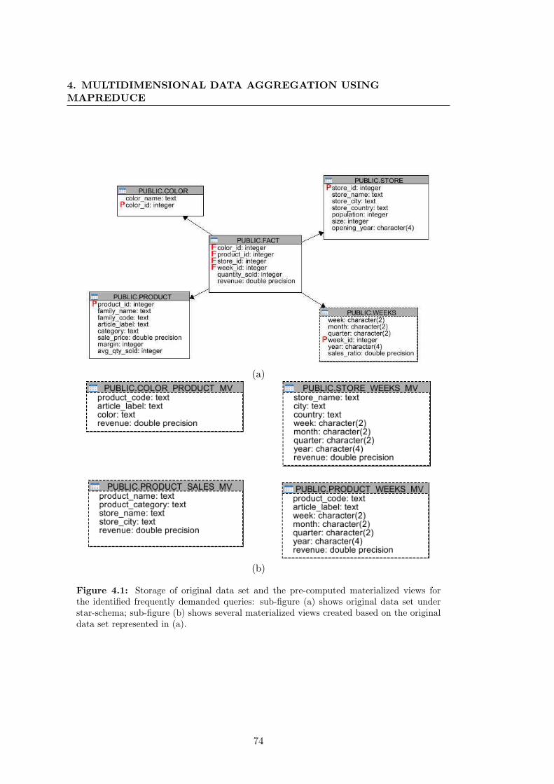
4. MULTIDIMENSIONAL DATA AGGREGATION USINGMAPREDUCE
(a)
(b)
Figure 4.1: Storage of original data set and the pre-computed materialized views forthe identified frequently demanded queries: sub-figure (a) shows original data set understar-schema; sub-figure (b) shows several materialized views created based on the originaldata set represented in (a).
74

4.2 Data Organization
Figure 4.2: Overall materialized view—ROWSET
s."store_country" AS store_state,
s."opening_year" AS opening_year,
w."week" AS week,
w."month" AS "month",
w."quarter" AS quarter,
w."year" AS "year",
f."quantity_sold" AS quantity_sold,
f."revenue" AS revenue
FROM "WEEKS" w JOIN
("COLOR" c JOIN
("PRODUCT" p JOIN
("STORE" s JOIN
"FACT" f ON (f."store_id"=s."store_id"))
ON (f."product_id"=p."product_id"))
ON (f."color_id"=c."color_id"))
ON (w."week_id"=f."week_id");
In this work, the data organization of single overall materialized view is adopted. It
has several advantages. Firstly, comparing with multiple materialized views approaches,
the required storage space is reduced. Secondly, the overall materialized view is not
created for optimizing a set of pre-chosen queries, instead, all queries can benefit from
this materialized view. Thirdly, with one materialized view, the emerging search engine
75

4. MULTIDIMENSIONAL DATA AGGREGATION USINGMAPREDUCE
techniques could be easily applied. In particular, in this work, one materialized view
approach greatly simplifies data partitioning and indexing work.
Term specification From now on, the terms dimension and measure are slightly
different from the recognized terms with common names in OLAP field. In order to
avoid confusion, we would like to newly declare the definitions of these two terms. If not
additionally specified, the following occurrences of the two terms adopt the definitions
below.
• Dimension is a type of columns, of which the distinct values are of type text.
• Measure is a type of columns, of which the distinct values are of type numeric.
To be noted, hierarchy is not adopted in this terminology.
4.3 Computations Involved in Data Explorations
In SAP BusinessObjects data explorer, user selects an information space, and then
enters into a relevant exploration panel. The first page displayed in exploration panel
shows aggregated measures dimension by dimension. User can selected various ag-
gregate functions, such as COUNT, SUM, AVERAGE, MAX, MIN, etc, by clicking
a drop-list. Assuming the aggregate function SUM applied on all the measures, then
the computations involved within the display of the first page actually is equivalent to
execution of SQL statement of the List 4.2.
Listing 4.2: SQL statements used for displaying the first page of exploration panel.
DROP VIEW IF EXISTS page_0 CASCADE;
CREATE VIEW page_0 AS
SELECT * FROM "ROWSET"
;
DROP VIEW IF EXISTS dimension_0;
CREATE VIEW dimension_0 AS
SELECT "page_0"."color" AS distinct_value,
SUM(page_0."quantity_sold") AS quantity_sold,
SUM(page_0."revenue") AS revenue
FROM "page_0"
GROUP BY "distinct_value"
;
DROP VIEW IF EXISTS dimension_1;
76
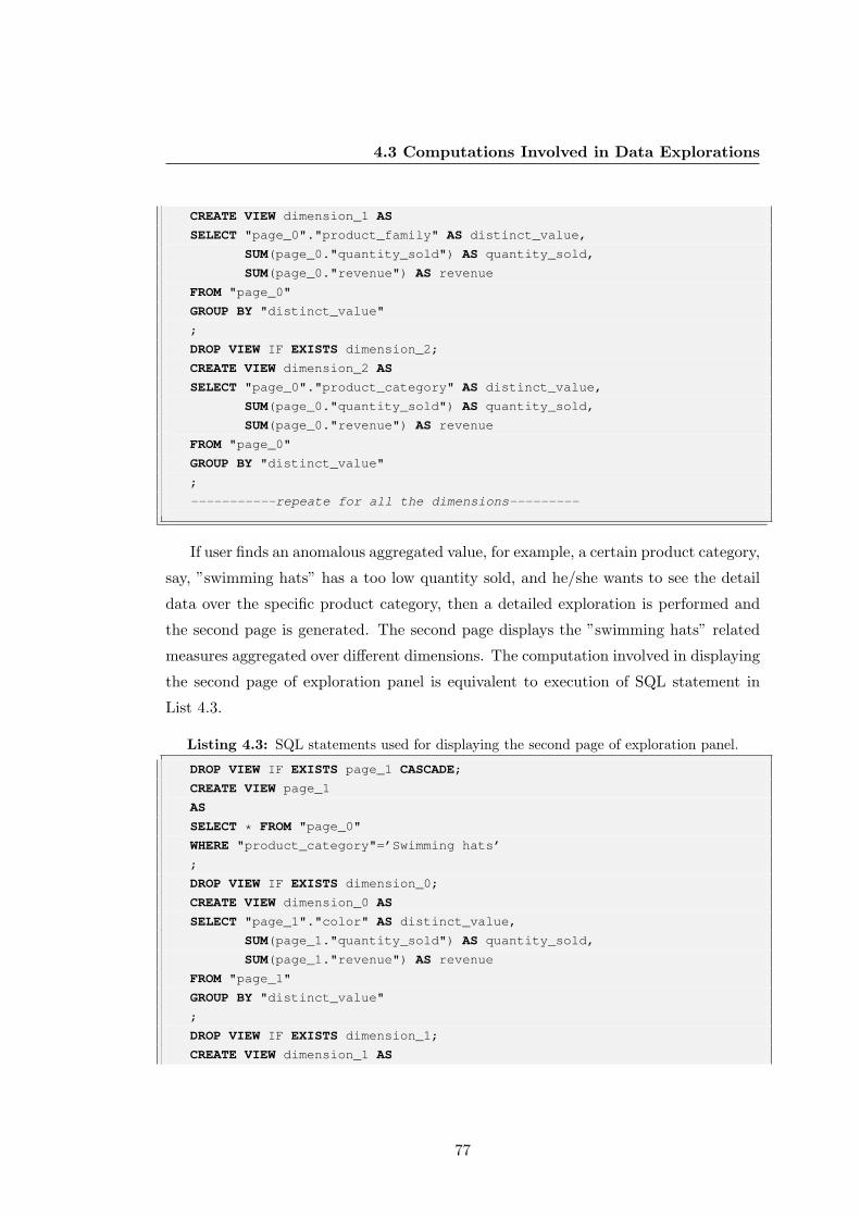
4.3 Computations Involved in Data Explorations
CREATE VIEW dimension_1 AS
SELECT "page_0"."product_family" AS distinct_value,
SUM(page_0."quantity_sold") AS quantity_sold,
SUM(page_0."revenue") AS revenue
FROM "page_0"
GROUP BY "distinct_value"
;
DROP VIEW IF EXISTS dimension_2;
CREATE VIEW dimension_2 AS
SELECT "page_0"."product_category" AS distinct_value,
SUM(page_0."quantity_sold") AS quantity_sold,
SUM(page_0."revenue") AS revenue
FROM "page_0"
GROUP BY "distinct_value"
;
-----------repeate for all the dimensions---------
If user finds an anomalous aggregated value, for example, a certain product category,
say, ”swimming hats” has a too low quantity sold, and he/she wants to see the detail
data over the specific product category, then a detailed exploration is performed and
the second page is generated. The second page displays the ”swimming hats” related
measures aggregated over different dimensions. The computation involved in displaying
the second page of exploration panel is equivalent to execution of SQL statement in
List 4.3.
Listing 4.3: SQL statements used for displaying the second page of exploration panel.
DROP VIEW IF EXISTS page_1 CASCADE;
CREATE VIEW page_1
AS
SELECT * FROM "page_0"
WHERE "product_category"=’Swimming hats’
;
DROP VIEW IF EXISTS dimension_0;
CREATE VIEW dimension_0 AS
SELECT "page_1"."color" AS distinct_value,
SUM(page_1."quantity_sold") AS quantity_sold,
SUM(page_1."revenue") AS revenue
FROM "page_1"
GROUP BY "distinct_value"
;
DROP VIEW IF EXISTS dimension_1;
CREATE VIEW dimension_1 AS
77
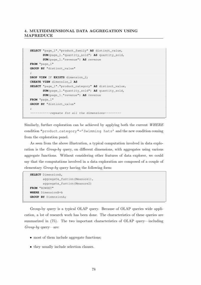
4. MULTIDIMENSIONAL DATA AGGREGATION USINGMAPREDUCE
SELECT "page_1"."product_family" AS distinct_value,
SUM(page_1."quantity_sold") AS quantity_sold,
SUM(page_1."revenue") AS revenue
FROM "page_1"
GROUP BY "distinct_value"
;
DROP VIEW IF EXISTS dimension_2;
CREATE VIEW dimension_2 AS
SELECT "page_1"."product_category" AS distinct_value,
SUM(page_1."quantity_sold") AS quantity_sold,
SUM(page_1."revenue") AS revenue
FROM "page_1"
GROUP BY "distinct_value"
;
-----------repeate for all the dimensions---------
Similarly, further exploration can be achieved by applying both the current WHERE
condition "product category"=’Swimming hats’ and the new condition coming
from the exploration panel.
As seen from the above illustration, a typical computation involved in data explo-
ration is the Group-by query, on different dimensions, with aggregates using various
aggregate functions. Without considering other features of data explorer, we could
say that the computations involved in a data exploration are composed of a couple of
elementary Group-by query having the following form:
SELECT DimensionA,
aggregate_funtion(Measure1),
aggregate_funtion(Measure2)
FROM "ROWSET"
WHERE DimensionB=b
GROUP BY DiemnsionA;
Group-by query is a typical OLAP query. Because of OLAP queries wide appli-
cation, a lot of research work has been done. The characteristics of these queries are
summarized in (75). The two important characteristics of OLAP query—including
Group-by query—are:
• most of them include aggregate functions;
• they usually include selection clauses.
78

4.4 Multiple Group-by Query
Going any further from the two characteristics, one Group-by query involves two pro-
cessing phases, filtering and aggregating. During filtering phase, the WHERE condition
is applied to filter the records of materialized view. During the aggregating phase, the
aggregate function is performed over the filtered records.
4.4 Multiple Group-by Query
For being able to response user’s exploration, multiple Group-by queries need to be
calculated simultaneously, instead of one single Group-by query. The term Multiple
Group-by query is able to more clearly express the characteristics of the query addressed
in this work. For defining the Multiple Group-by query, we describe it as follows:
Multiple Group-By query is a set of Group-by queries using the same select-where
clause block. More formally, Multiple Group-By query can be expressed in SQL with
the following form:
SELECT X, SUM(*),
FROM R WHERE condition
GROUP BY X
ORDER BY X;
where X is a set of columns on relation R.
Some commercial database systems support a similar Group-by construct named
GROUPING SETS, and it allows the computation of multiple Group-by queries using
a single SQL statement (111). Comparing with the Multiple Group by query addressed
in this work, GROUPING SETS query is slightly different. Each Group-by query
contained in GROUPING SETS query could have more than one group-by dimension,
i.e. one Group-by query aggregates over more than one dimension, whereas in this
work, one Group-by query aggregates over only one dimension.
4.5 Challenges
In data exploration environment, processing Multiple Group-by query has several chal-
lenges. The first challenge is large data volume. In a very common case, the historical
data set is often of large size. The generated materialized view also is of large size. In
79

4. MULTIDIMENSIONAL DATA AGGREGATION USINGMAPREDUCE
order for user to do analysis as comprehensively as possible, the historical data set con-
tains many dimensions. It is not rare that the generated overall materialized view has
more than 10 dimensions. The second challenge is the requirement of short response
time. It is a common demand for all the interactive interface application, including data
exploration. Multiple Group-by queries aggregating over all dimensions is repeatedly
invoked and processed during data exploration, then it is required that each query is
answer within a very short time, for example, not more than 5 seconds, ideally, within
hundreds of milliseconds. Summarizing these challenges’ description—doing time and
resource consuming computations in short time.
Parallelization is the solution to address these challenges: partition the large ma-
terialized view ROWSET into smaller blocks, then processed query over each of them,
finally merge the results. One particular thing of this work is that we utilize cheap
commodity hardware instead of expensive supercomputer. This is also the significant
side of this work. This particularity brings further challenges, scalability and fault
tolerance issues. For addressing these challenges, we adopt MapReduce model, and the
detailed specifications will be given later in this chapter.
4.6 Choosing a Right MapReduce Framework
There exist several researches and projects focusing on building specific MapReduce
frameworks for various hardware and different distributed architectures. In our work,
we adopt the shared-nothing clusters, which are available for free1. Some well-designed
MapReduce frameworks are already realized for this type of hardware architecture. We
need to the right framework for satisfying the specific requirement.
4.6.1 GridGain Wins by Low-latency
Interactivity, i.e. short response time is the basic requirement in this work. In order
to meet this requirement, while the application-level optimization is essential, choosing
a right underlying MapReduce framework is also important. At our framework choos-
ing moment, there were two different open-source MapReduce frameworks available,
Hadoop (11) and GridGain (10).
1Grid’5000, for more information, refer to(9)
80
4.6 Choosing a Right MapReduce Framework
At first, Hadoop has been chosen as the MapReduce supporting framework. We
successfully installed and configured Hadoop in a cluster of two computers, and run
several simple tests over Hadoop. The experiment execution time over Hadoop was
not satisfying. An application of filtering materialized view of small size with a given
condition took already several seconds, which is too slow for interactive interface. This
phenomenon was then diagnosed as a consequence of the high latency of Hadoop. Ac-
tually, high latency is consistent with the initial design of Hadoop. Hadoop is designed
to address batch-processing application. Batch-processing application only emphasizes
high-throughput. In such a context, high-latency is insignificant. The high-latency is
also a side effect of Hadoop’s ”MapReduce + HDFS” design, of which more explanation
can be found in Subsection 3.1.2.
Another MapReduce framework, GridGain, is finally adopted as the underlying
framework in this work. GridGain offers a low latency since it is a pure MapReduce
engine without being associated with a distributed file system. Therefore, data par-
titioning and distributing should be manually managed. Although this increases the
workload of programmers, they have a chance to do optimizations at the data access
level. Additionally, GridGain provides several pre-defined scheduling policies including
data affinity scheduling policy, which can be beneficial for processing multiple contin-
uous queries.
4.6.2 Terminology
In GridGain, a Task is a MapReduce processing procedure; a Job is either a Map
procedure or a Reduce procedure. In Hadoop, the two terms are used inversely. A
MapReduce procedure is called a Job in Hadoop, and a Map or a Reduce procedure is
called a Task. In this dissertation, we adopt the terminology of GridGain.
4.6.3 Combiner Support in Hadoop and GridGain
Combiner is an optional component, which is located between the mapper and the
reducer. In Hadoop, combiner component is implemented, and user can choose to use
or not to use it freely. The combiner is physically located on each computing node.
Its function is to locally collect the intermediate output from the mappers running on
current node before these intermediate outputs being sent over the network. In certain
81

4. MULTIDIMENSIONAL DATA AGGREGATION USINGMAPREDUCE
Figure 4.3: Create the task of MapCombineReduce model by combining two GridGainMapReduce tasks.
case, using this combiner component can optimize the performance of the entire model.
The objective of using combiner is to reduce the intermediate data transfer.
This optional component combiner is not implemented in GridGain. In this work,
we propose a bypass method to make GridGain supporting combiner. Although this
method is implemented on top of GridGain, it is not limited to work with GridGain.
The same idea can also be carried out on other MapReduce frameworks. We illustrate
this method in the Figure 4.3. A GridGain MapReduce is composed of multiple mappers
and one reducer. In this method, we utilized two successive GridGain MapReduce
tasks. In the first MapReduce task, the mappers correspond to the mapper component
of MapCombineReduce model, and its reducer acts as a trigger to activate the second
MapReduce task, once the first MapReduce’s mappers have all finished their works.
The mappers of the second MapReduce task actually act as the combiner component
of MapCombineReduce model. The reducer of the second MapReduce task does the
job of the reducer component of MapCombineReduce model.
4.6.4 Realizing MapReduce Applications with GridGain
GridGain provides developers with Java-based technologies to develop and to run grid
applications on private or public clouds. In order to implement a MapReduce ap-
plication, there are mainly two classes need to define in GridGain, i.e. Task, and
82
4.6 Choosing a Right MapReduce Framework
Job. Task class’s definition requires developer realizing map() and reduce() func-
tions. Job class’s definition requires developer realizing execute() function. The
name of map() might be confusing. This name misleads people to think it defines the
calculations to be carried out in mapper. But in fact, the map() function is respon-
sible for establishing the mappings between mappers and worker nodes. This function
could be utilized to apply user-defined job-scheduling policy. GridGain provides some
pre-defined implementations of map() function, which support various job-scheduling
policies, including data affinity, round robin, weighted random, etc. The web site
of GridGain (10) gives to the readers more descriptions about GridGain’s supported
job-scheduling policies. execute() is actually the function specifying operations per-
formed by mapper. execute() contains the distributed computations which will be
executed in parallel with other instances of execute() function. When a mapper arrives
at a remote worker node, a collision resolving strategy will look into a queue of existing
mappers on this worker node to either reject the current mapper or leave it waiting
in the queue. When the mapper got run, the execute() function will be executed.
Reduce function contains the actions of reducer, collecting mappers intermediate out-
puts and calculate the final result. It usually is composed of some aggregate-type
operations. Reduce() function’s execution is activated by the arrival of the mappers’
intermediate outputs. According to the policy defined by the user, reduce() can be
activated once the first intermediate output from mapper arrives at the master node,
or after the sub-results of all the mappers arrived. The default policy is to wait all the
mappers to finish their works and then to activate the reduce() method. In addition,
developer also need to define a task loader program, which takes charge of initializing
the parameters, starting a grid instance, launching user’s application, and then waiting
and collecting the results.
4.6.5 Workflow Analysis of GridGain MapReduce Procedure
GridGain’s MapReduce is composed of multiple mappers and one reducer. The mappers
are sent to and run on worker nodes, and the reducer run on master node. For fully
understanding the procedure of GridGain’s MapReduce, we analyzed the log file of
GridGain and also did the profiling work when running MapReduce application. The
following description of GridGain MapReduce workflow is based on this analysis.
83

4. MULTIDIMENSIONAL DATA AGGREGATION USINGMAPREDUCE
The Figure 4.4 shows the workflow of a GridGain’s MapReduce task. When master
starts a MapReduce task, it in fact starts a thread for this task. The thread does the
start-up work and closure work for the task. The start-up work includes the following
steps.
1. Firstly, master creates mappings between user-defined jobs (mappers) and avail-
able worker nodes;
2. Secondly, master serializes mappers in a sequential way ;
3. Once all mappers are serialized, master sends each mapper to the corresponding
worker node.
After all the mappers being sent, the thread terminates and the master enters into
a ”waiting” status. This ”waiting” status continues until the master node receives the
mappers’ intermediate outputs. When the master node receives a mapper’s intermedi-
ate output, it begins to de-serialize this intermediate output immediately. After all the
intermediate outputs are de-serialized, then it starts the reducer. The de-serialization
and reducer execution compose the task’s closure.
On the other side, the worker node listens to the messages after the GridGain
instance is started. When it receives a message containing serialized mapper object, it
will de-serialize the message, thereby it obtains mapper’s object. Then, the mapper is
put into a queue waiting for being executed once one or more CPU becomes available.
After the mapper’s execution is accomplished, the intermediate output is serialized and
sent back to the master node.
4.7 Paralleling Single Group-by Query with MapReduce
Before addressing the parallelization of Multiple Group-by query, we describe the pro-
cessing of the elementary query—single Group-by query—in MapReduce. Intuitively,
single Group-by query could be well matched with MapReduce model. A single Group-
by query can be executed in two phases: the first phase is filtering, and the second
phase is aggregating. The other operations (regroup) can be incorporated into the ag-
gregating phase. The filtering phase corresponds to the mapper’work in MapReduce,
and the aggregating phase corresponds to its reducer’s work.
84
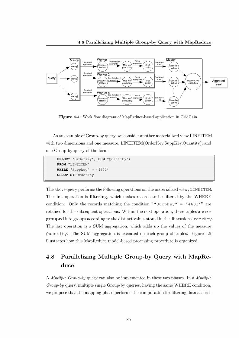
4.8 Parallelizing Multiple Group-by Query with MapReduce
Figure 4.4: Work flow diagram of MapReduce-based application in GridGain.
As an example of Group-by query, we consider another materialized view LINEITEM
with two dimensions and one measure, LINEITEM(OrderKey,SuppKey,Quantity), and
one Group-by query of the form:
SELECT "Orderkey", SUM("Quantity")
FROM "LINEITEM"
WHERE "Suppkey" = ’4633’
GROUP BY Orderkey
The above query performs the following operations on the materialized view, LINEITEM.
The first operation is filtering, which makes records to be filtered by the WHERE
condition. Only the records matching the condition ”"Suppkey" = ’4633’” are
retained for the subsequent operations. Within the next operation, these tuples are re-
grouped into groups according to the distinct values stored in the dimension OrderKey.
The last operation is a SUM aggregation, which adds up the values of the measure
Quantity. The SUM aggregation is executed on each group of tuples. Figure 4.5
illustrates how this MapReduce model-based processing procedure is organized.
4.8 Parallelizing Multiple Group-by Query with MapRe-
duce
A Multiple Group-by query can also be implemented in these two phases. In a Multiple
Group-by query, multiple single Group-by queries, having the same WHERE condition,
we propose that the mapping phase performs the computation for filtering data accord-
85
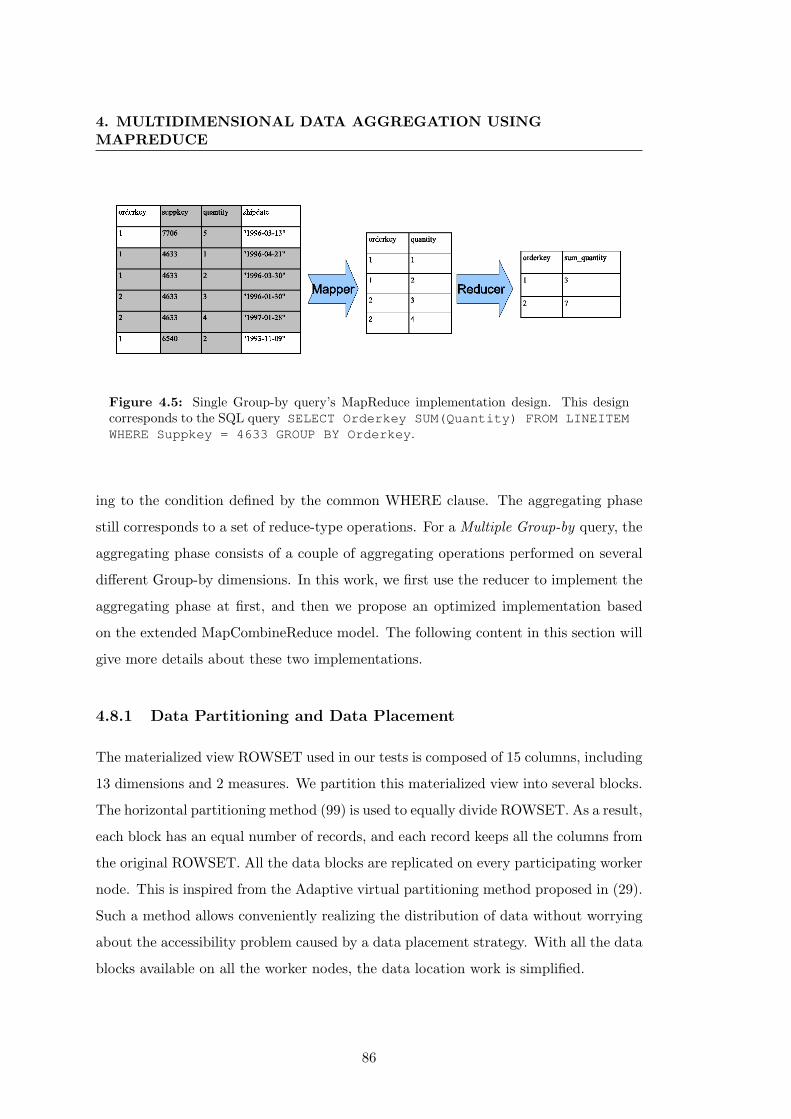
4. MULTIDIMENSIONAL DATA AGGREGATION USINGMAPREDUCE
Figure 4.5: Single Group-by query’s MapReduce implementation design. This designcorresponds to the SQL query SELECT Orderkey SUM(Quantity) FROM LINEITEM
WHERE Suppkey = 4633 GROUP BY Orderkey.
ing to the condition defined by the common WHERE clause. The aggregating phase
still corresponds to a set of reduce-type operations. For a Multiple Group-by query, the
aggregating phase consists of a couple of aggregating operations performed on several
different Group-by dimensions. In this work, we first use the reducer to implement the
aggregating phase at first, and then we propose an optimized implementation based
on the extended MapCombineReduce model. The following content in this section will
give more details about these two implementations.
4.8.1 Data Partitioning and Data Placement
The materialized view ROWSET used in our tests is composed of 15 columns, including
13 dimensions and 2 measures. We partition this materialized view into several blocks.
The horizontal partitioning method (99) is used to equally divide ROWSET. As a result,
each block has an equal number of records, and each record keeps all the columns from
the original ROWSET. All the data blocks are replicated on every participating worker
node. This is inspired from the Adaptive virtual partitioning method proposed in (29).
Such a method allows conveniently realizing the distribution of data without worrying
about the accessibility problem caused by a data placement strategy. With all the data
blocks available on all the worker nodes, the data location work is simplified.
86
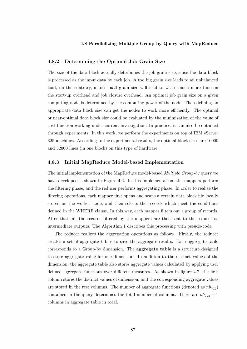
4.8 Parallelizing Multiple Group-by Query with MapReduce
4.8.2 Determining the Optimal Job Grain Size
The size of the data block actually determines the job grain size, since the data block
is processed as the input data by each job. A too big grain size leads to an unbalanced
load, on the contrary, a too small grain size will lead to waste much more time on
the start-up overhead and job closure overhead. An optimal job grain size on a given
computing node is determined by the computing power of the node. Then defining an
appropriate data block size can get the nodes to work more efficiently. The optimal
or near-optimal data block size could be evaluated by the minimization of the value of
cost function working under current investigation. In practice, it can also be obtained
through experiments. In this work, we perform the experiments on top of IBM eServer
325 machines. According to the experimental results, the optimal block sizes are 16000
and 32000 lines (in one block) on this type of hardware.
4.8.3 Initial MapReduce Model-based Implementation
The initial implementation of the MapReduce model-based Multiple Group-by query we
have developed is shown in Figure 4.6. In this implementation, the mappers perform
the filtering phase, and the reducer performs aggregating phase. In order to realize the
filtering operations, each mapper first opens and scans a certain data block file locally
stored on the worker node, and then selects the records which meet the conditions
defined in the WHERE clause. In this way, each mapper filters out a group of records.
After that, all the records filtered by the mappers are then sent to the reducer as
intermediate outputs. The Algorithm 1 describes this processing with pseudo-code.
The reducer realizes the aggregating operations as follows. Firstly, the reducer
creates a set of aggregate tables to save the aggregate results. Each aggregate table
corresponds to a Group-by dimension. The aggregate table is a structure designed
to store aggregate value for one dimension. In addition to the distinct values of the
dimension, the aggregate table also stores aggregate values calculated by applying user
defined aggregate functions over different measures. As shown in figure 4.7, the first
column stores the distinct values of dimension, and the corresponding aggregate values
are stored in the rest columns. The number of aggregate functions (denoted as nbagg)
contained in the query determines the total number of columns. There are nbagg + 1
columns in aggregate table in total.
87
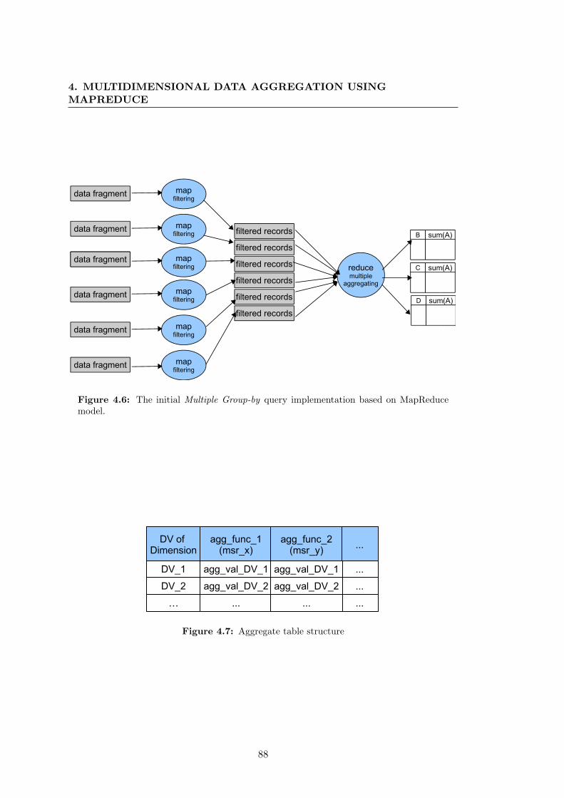
4. MULTIDIMENSIONAL DATA AGGREGATION USINGMAPREDUCE
Figure 4.6: The initial Multiple Group-by query implementation based on MapReducemodel.
Figure 4.7: Aggregate table structure
88
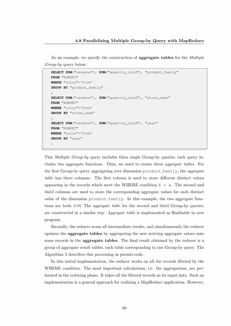
4.8 Parallelizing Multiple Group-by Query with MapReduce
As an example, we specify the construction of aggregate tables for the Multiple
Group-by query below:
SELECT SUM("revenue"), SUM("quantity_sold"), "product_family"
FROM "ROWSET"
WHERE "color"=’Pink’
GROUP BY "product_family"
;
SELECT SUM("revenue"), SUM("quantity_sold"), "store_name"
FROM "ROWSET"
WHERE "color"=’Pink’
GROUP BY "store_name"
;
SELECT SUM("revenue"), SUM("quantity_sold"), "year"
FROM "ROWSET"
WHERE "color"=’Pink’
GROUP BY "year"
;
This Multiple Group-by query includes three single Group-by queries; each query in-
cludes two aggregate functions. Thus, we need to create three aggregate tables. For
the first Group-by query aggregating over dimension product family, the aggregate
table has three columns. The first column is used to store different distinct values
appearing in the records which meet the WHERE condition E > e. The second and
third columns are used to store the corresponding aggregate values for each distinct
value of the dimension product family. In this example, the two aggregate func-
tions are both SUM. The aggregate table for the second and third Group-by queries,
are constructed in a similar way. Aggregate table is implemented as Hashtable in over
program.
Secondly, the reducer scans all intermediate results, and simultaneously the reducer
updates the aggregate tables by aggregating the new arriving aggregate values onto
some records in the aggregate tables. The final result obtained by the reducer is a
group of aggregate result tables, each table corresponding to one Group-by query. The
Algorithm 2 describes this processing in pseudo-code.
In this initial implementation, the reducer works on all the records filtered by the
WHERE condition. The most important calculations, i.e. the aggregations, are per-
formed in the reducing phase. It takes all the filtered records as its input data. Such an
implementation is a general approach for realizing a MapReduce application. However,
89
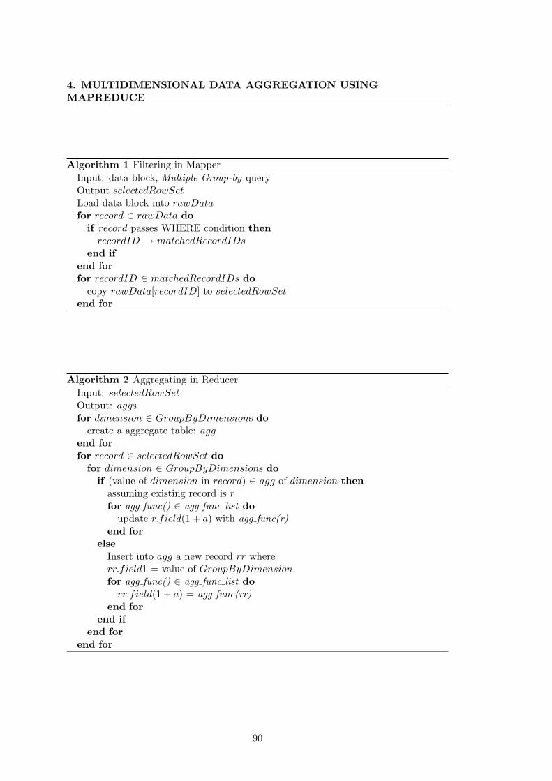
4. MULTIDIMENSIONAL DATA AGGREGATION USINGMAPREDUCE
Algorithm 1 Filtering in Mapper
Input: data block, Multiple Group-by queryOutput selectedRowSetLoad data block into rawDatafor record ∈ rawData do
if record passes WHERE condition thenrecordID → matchedRecordIDs
end ifend forfor recordID ∈ matchedRecordIDs do
copy rawData[recordID] to selectedRowSetend for
Algorithm 2 Aggregating in Reducer
Input: selectedRowSetOutput: aggsfor dimension ∈ GroupByDimensions do
create a aggregate table: aggend forfor record ∈ selectedRowSet do
for dimension ∈ GroupByDimensions doif (value of dimension in record) ∈ agg of dimension then
assuming existing record is rfor agg func() ∈ agg func list do
update r.field(1 + a) with agg func(r)end for
elseInsert into agg a new record rr whererr.field1 = value of GroupByDimensionfor agg func() ∈ agg func list do
rr.field(1 + a) = agg func(rr)end for
end ifend for
end for
90

4.8 Parallelizing Multiple Group-by Query with MapReduce
it is not fully suitable for GridGain. Because of the limitation of GridGain (only one
reducer), all the filtered records should be transfer over the network. This could cause
high overhead when the bandwidth is limited.
4.8.4 MapCombineReduce Model-based Optimization
In the initial implementation, all the intermediate outputs produced by the mappers
(i.e. all the records matching the WHERE condition), are sent to the reducer over the
network. If query selectivity 1 under the given WHERE condition is relatively small,
for instance 1%2, then output of mapping phase will be moderate, and the initial
implementation is suitable. However, if the query selectivity is larger, for instance,
9%, then the number of records will be great and the volume of data being transferred
over the network will become large, which causes a higher communication cost. As a
consequence, the initial implementation is not suitable for queries with relatively large
selectivity.
In order to reduce the network overhead caused by the intermediate data transmis-
sion for queries with larger selectivity value, we propose a MapCombineReduce model-
based implementation. We let the combiner component to act as a pre-aggregator
on each worker node. In this work, the number of combiner of each worker node is
one. In optimized MapCombineReduce model-based implementation, the mapper first
performs the same operations of the filtering phase as in the initial implementation.
However, the result of the filtering phase will be put into the local cache instead of
being sent over the network immediately. The mapper then sends out a signal when it
finished its work. The trigger (i.e. reducer in the first MapReduce task) will receive
this signal. When the trigger receives all the work finished signals, then it activates the
second MapReduce task. In the second MapReduce task, the combiner (i.e. the map-
per of the second MapReduce task) does the aggregating operations locally within each
worker node. Each of the combiners generates a portion of aggregate the results, i.e. a
set of partial aggregate tables. Then they send out their partial results to the reducer.
After merging all the partial results, the reducer generates the final aggregate tables
of the Multiple Group-by query. Thus, the volume of data to be transferred is reduced
1Here, a selectivity of a select query means the ratio value between the number of records satisfyingthe predicate defined in the WHERE clause and the cardinality of the relation.
2This means that only 1% of the records are selected out from the data source table.
91
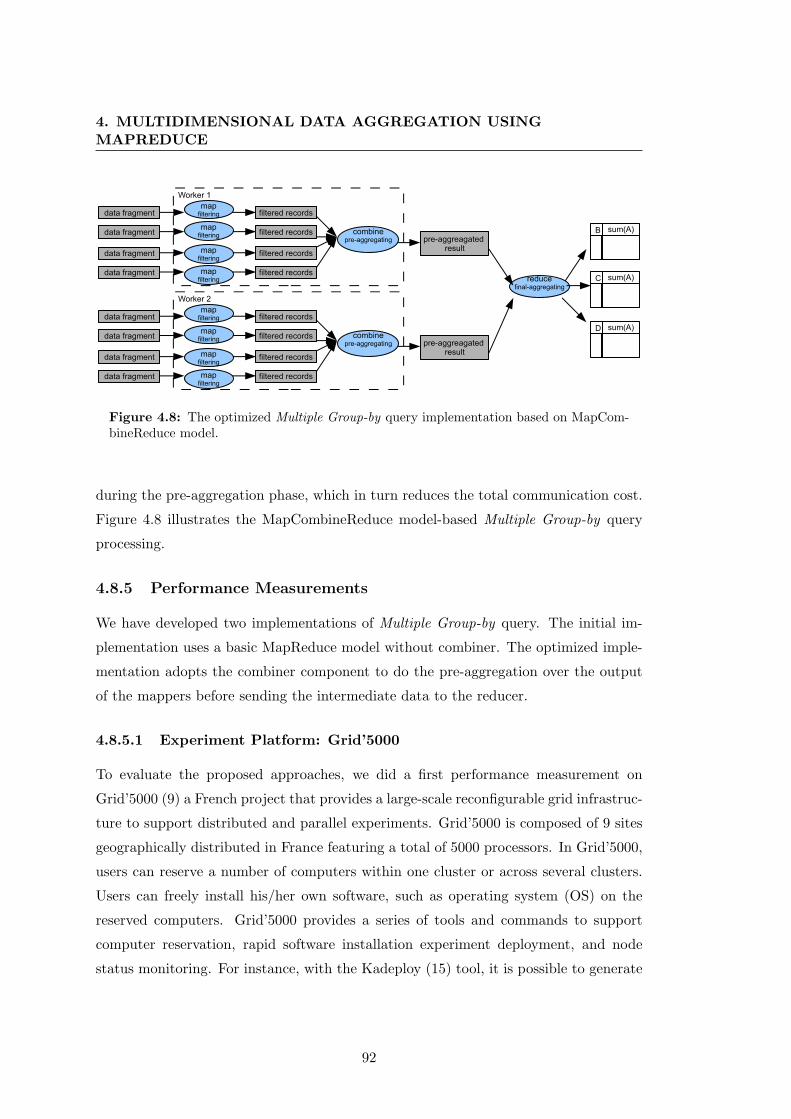
4. MULTIDIMENSIONAL DATA AGGREGATION USINGMAPREDUCE
Figure 4.8: The optimized Multiple Group-by query implementation based on MapCom-bineReduce model.
during the pre-aggregation phase, which in turn reduces the total communication cost.
Figure 4.8 illustrates the MapCombineReduce model-based Multiple Group-by query
processing.
4.8.5 Performance Measurements
We have developed two implementations of Multiple Group-by query. The initial im-
plementation uses a basic MapReduce model without combiner. The optimized imple-
mentation adopts the combiner component to do the pre-aggregation over the output
of the mappers before sending the intermediate data to the reducer.
4.8.5.1 Experiment Platform: Grid’5000
To evaluate the proposed approaches, we did a first performance measurement on
Grid’5000 (9) a French project that provides a large-scale reconfigurable grid infrastruc-
ture to support distributed and parallel experiments. Grid’5000 is composed of 9 sites
geographically distributed in France featuring a total of 5000 processors. In Grid’5000,
users can reserve a number of computers within one cluster or across several clusters.
Users can freely install his/her own software, such as operating system (OS) on the
reserved computers. Grid’5000 provides a series of tools and commands to support
computer reservation, rapid software installation experiment deployment, and node
status monitoring. For instance, with the Kadeploy (15) tool, it is possible to generate
92

4.8 Parallelizing Multiple Group-by Query with MapReduce
customized images of operating systems and applications, store and automatically or
interactively load them through the job scheduler tool OAR (17).
For the experiments in this work, we ran the version 2.1.1 of GridGain over Java
1.6.0 on top of computers in one cluster located in the Sophia site. In this cluster, all
the computers are of model IBM eServer 325. The total number of nodes in this cluster
is 49 and each node is equipped with two AMD Opteron 246 2.0GHz processors, 2GB of
RAM and network card of Myrinet-2000, running under the 64-bit Debian. We reserve
from 1 to 20 nodes according to the experiment requirements. GridGain instances
are started at master node and worker nodes, the JVM maximum of heap size were
set to 1536MB. In the following experiments, we were mainly interested in the two
performance aspects of our Multiple Group-by query implementations, the speed-up
and the scalability.
4.8.5.2 Speed-up
In our work, the materialized view was stored as a plain text CSV file. We use a
materialized view of 640 000 records which is composed of 15 columns, including 13
dimensions and 2 measures. Each record is stored as a different line of the CSV file.
We partitioned this materialized view with 5 different block sizes: 1000, 2000, 4000,
8000 and 16000. Several Multiple Group-by queries with different selectivities1 (1.06%,
9.9%, 18.5%) were executed on the materialized view. Each query includes 7 Group-by
queries. In order to test the speed-up, We firstly ran a sequential test on one machine in
the cluster, then we launched the parallel tests realized with GridGain on 5, 10, then on
15, and finally on 20 worker nodes. Each test is run 5 times and the average execution
time was recorded. Figure 4.9 shows the speed-up of the initial implementation and
the optimized one comparing with the sequential execution time.
As seen from this figure, no good speed-up is obtained with small block sizes such
as 1000 and 2000. However, an obvious acceleration can be observed when using larger
block size like 4000, 8000 and 16000. The explanation of this phenomenon is that, for
each job running on a worker node, there are some initial costs to start (job start-up)
and to close the job (job closure). The actions in job start-up include receiving data
or parameters from the calling node (usually this is the master node), preparing the
1The selectivity of a select query means the ratio value between the number of records satisfyingthe predicate defined in the WHERE clause and the cardinality of the relation
93

4. MULTIDIMENSIONAL DATA AGGREGATION USINGMAPREDUCE
Figure 4.9: Speed-up versus the number of machines and the block size (1000, 2000, 4000,8000, 16000).
94
4.8 Parallelizing Multiple Group-by Query with MapReduce
input data or reading the input data from an indicated place, etc. The job closure cost
consists in establishing a connection with the master node in order to send back the
intermediate outputs on worker side, and receiving and pre-processing each intermediate
output on the master side. The smaller the block size is, the larger the job number is.
When the block size is equal to 1000 or 2000, the number of jobs is large and the job
start-up/closure cost becomes important . . .
The results shown in the two first figures consider a query with selectivity equal to
1.06%. With this small selectivity, the output of the mappers is not large enough, and
the optimized implementation does not exhibit its advantage over the initial implemen-
tation. However, increasing the query selectivity (e.g. 9.9% and 18.5%), makes the in-
termediate data being transferred in the initial implementation considerably larger than
those transferred in the optimized implementation. As a consequence, the optimized
implementation shows a better speed-up performance than the initial implementation.
4.8.5.3 Scalability
For the scalability, we used several materialized views having the same dimensions
and measures, but containing several times more records than the one of the speed-up
tests. We used materialize views of 640 000, 1 280 000, 1 920 000 and 2560000 records,
respectively. The tests performed using the materialized view of 640 000 records were
run on 5 machines, those using the materialized view of 1 280 000 records were run
on 10 machines, those using materialized view of 1 920 000 records were run on 15
machines, and those using materialized view of 2 560 000 records were run on 20
machines. According to the previous test case, the executions with block size as 16000
had better performance than the other ones. Therefore, we defined the block size of
16000, and we used queries with the same selectivities as used in speed-up experiments.
Figure 4.10 shows the obtained results.
These figures show that the optimized implementation has very good scalability.
With an increasing the data scale, the executions spend almost the same time (the
difference is smaller than 1 seconds). As seen from the first figure, for the case of query
selectivity equal to 1.06%, the workload is relatively small and both the optimized
implementation and the initial implementation gave acceptable execution time, i.e.
within 3 seconds. Note that in case of a small selectivity, the communication cost
was not dominant and the pre-aggregation work did not bring an obvious optimizing
95

4. MULTIDIMENSIONAL DATA AGGREGATION USINGMAPREDUCE
Figure 4.10: Comparison of the execution time upon the size of the data set and thequery selectivity.
effect. In the rest of the figures, the query selectivities have larger values. This enables
more records to be selected and implies larger communication costs for transferring
intermediate output. As a consequence, the optimized implementation always shows
better performance than the initial implementation, and the curve if the optimized
implementation stands upper the curve of the initial implementation. This behaviour
is clearly outlined for query selectivity equal to 9.9% and 18.5%.
4.9 Execution Time Analysis
In this section, we will describe a basic analysis of execution time of the Multiple Group-
by query. These cost analysis respectively address the initial implementation based on
the MapReduce and optimized implementation based on the MapCombineReduce. As
96

4.9 Execution Time Analysis
mentioned earlier, a GridGain MapReduce task’s calculation is composed of the start-
up and closure on the master node, and the mapper executions over worker nodes. In
this work, we are also interested in the optimization over communication cost, thus,
communication time is considered, but we ignore the extra cost brought by the resource
contention over each worker node when running multiple mappers.
4.9.1 Cost Analysis for Initial Implementation
Assume that the Multiple Group-by query runs over a materialized view of N records,
and the query has nbGB Group-by dimensions. We use MapReduce-based method
to parallelize query processing. The parallel Multiple Group-by query’s total cost is
composed of four parts:
• start-up cost(on master node), denoted as Cst;
• mapper’s execution (on workers), denoted as Cm;
• closure cost (on master node), denoted as Ccl;
• communication cost, denoted as Ccmm.
In start-up, the master does the preparation of mappers, including the mappings
from mappers to available worker nodes, and then sequentially performs the serializa-
tions of mappers with their attached arguments. We use Cmpg to denote the time for
building mapping between mappers and worker nodes, Cs the time for serializing one
unit size of data, sizem the size of mapper object, nbm the number of mappers. The
notations that are used for expressing the cost analysis are listed in the Table 4.1.
Without considering the low-level details of serialization1, we simply assume that
the serialization time is proportional to the size of data being serialized, i.e. a bigger
mapper object consumes more time during the serialization. Therefore, a MapReduce
task of GridGain, the start-up cost Cst over master node is:
Cst = (Cmpg + Cs · sizem) · nbm
When a worker node receives a message containing mapper, it first serializes the
mapper as well as its arguments, it then launches the execution of mapper. When
1The details of serialization will be discussed in Chapter 5.
97
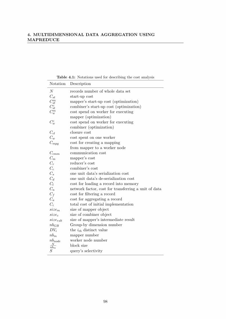
4. MULTIDIMENSIONAL DATA AGGREGATION USINGMAPREDUCE
Table 4.1: Notations used for describing the cost analysis
Notation Description
N records number of whole data setCst start-up costCm
st mapper’s start-up cost (optimization)Cc
st combiner’s start-up cost (optimization)Cm
w cost spend on worker for executingmapper (optimization)
Ccw cost spend on worker for executing
combiner (optimization)Ccl closure costCw cost spent on one workerCmpg cost for creating a mapping
from mapper to a worker nodeCcmm communication costCm mapper’s costCr reducer’s costCc combiner’s costCs one unit data’s serialization costCd one unit data’s de-serialization costCl cost for loading a record into memoryCn network factor, cost for transferring a unit of dataCf cost for filtering a recordCa cost for aggregating a recordCi total cost of initial implementationsizem size of mapper objectsizec size of combiner objectsizerslt size of mapper’s intermediate resultnbGB Group-by dimension numberDVi the ith distinct valuenbm mapper numbernbnode worker node number
Nnbm
block size
S query’s selectivity
98
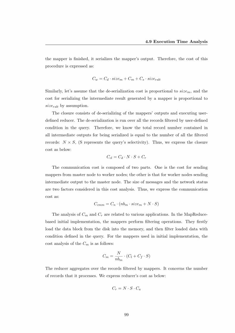
4.9 Execution Time Analysis
the mapper is finished, it serializes the mapper’s output. Therefore, the cost of this
procedure is expressed as:
Cw = Cd · sizem + Cm + Cs · sizerslt
Similarly, let’s assume that the de-serialization cost is proportional to sizem, and the
cost for serializing the intermediate result generated by a mapper is proportional to
sizerslt by assumption.
The closure consists of de-serializing of the mappers’ outputs and executing user-
defined reducer. The de-serialization is run over all the records filtered by user-defined
condition in the query. Therefore, we know the total record number contained in
all intermediate outputs for being serialized is equal to the number of all the filtered
records: N × S, (S represents the query’s selectivity). Thus, we express the closure
cost as below:
Ccl = Cd ·N · S + Cr
The communication cost is composed of two parts. One is the cost for sending
mappers from master node to worker nodes; the other is that for worker nodes sending
intermediate output to the master node. The size of messages and the network status
are two factors considered in this cost analysis. Thus, we express the communication
cost as:
Ccmm = Cn · (nbm · sizem + N · S)
The analysis of Cm and Cr are related to various applications. In the MapReduce-
based initial implementation, the mappers perform filtering operations. They firstly
load the data block from the disk into the memory, and then filter loaded data with
condition defined in the query. For the mappers used in initial implementation, the
cost analysis of the Cm is as follows:
Cm =N
nbm· (Cl + Cf · S)
The reducer aggregates over the records filtered by mappers. It concerns the number
of records that it processes. We express reducer’s cost as below:
Cr = N · S · Ca
99

4. MULTIDIMENSIONAL DATA AGGREGATION USINGMAPREDUCE
With the mapper and reducer’s cost analysis, we obtain the total cost analysis of the
initial implementation. We consider that mapper object’s size is small comparing with
the intermediate outputs, and it can be ignored when the data set is large, the costs
concerning mappers’ mapping, serialization, de-serializations and transmission can be
removed. Thus, the analysis as below is obtained:
Ci =N
nbm· (Cl + Cf · S) + Cs · sizerslt + (Cd + Ca + Cn) ·N · S (1)
4.9.2 Cost Analysis for Optimized Implementation
For MapCombineReduce-based optimization of multiple-group-by query, the total cost
is considered to be composed of:
• Mapper’s start-up (on master), denoted as Cmst ;
• Cost spend on one worker for executing a mapper, denoted as Cmw ;
• Combiners’ start-up (on master), denoted as Ccst;
• Cost spend on one worker for executing a combiner, denoted as Ccw;
• Closure (on master), denoted as Ccl;
• Communication, denoted as Ccmm.
The start-up of mappers is similar to that of MapReduce, we mark two superscripts m
and c in order to distinguish mapper’s start-up from combiner’s start-up:
Cmst = (Cmpg + Cs · sizem) · nbm
The mappers do the same calculations as in initial implementation. However, the
output’s size of each mapper is estimated as 0, because the mapper stores the selected
records into the worker’s memory and returns null. Thus, the cost for running a mapper
is expressed as below:
Cmw = Cd · sizem + Cm + 0
where
Cm =N
nbm· (Cl + Cf · S)
100
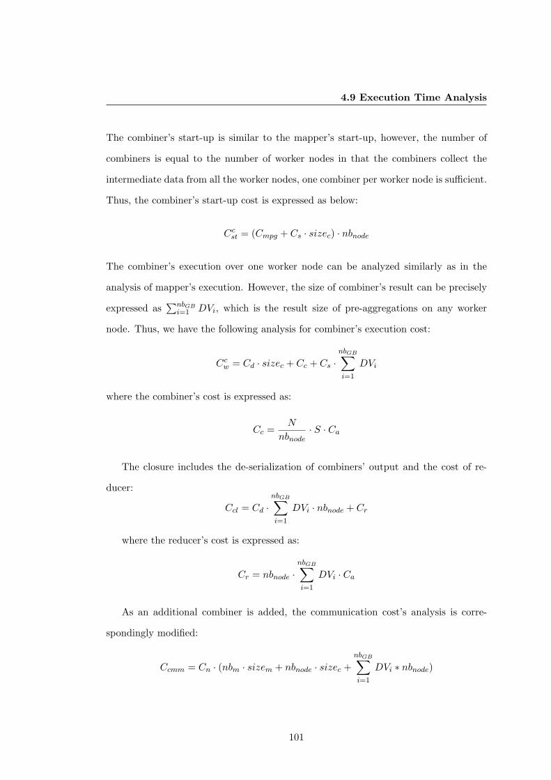
4.9 Execution Time Analysis
The combiner’s start-up is similar to the mapper’s start-up, however, the number of
combiners is equal to the number of worker nodes in that the combiners collect the
intermediate data from all the worker nodes, one combiner per worker node is sufficient.
Thus, the combiner’s start-up cost is expressed as below:
Ccst = (Cmpg + Cs · sizec) · nbnode
The combiner’s execution over one worker node can be analyzed similarly as in the
analysis of mapper’s execution. However, the size of combiner’s result can be precisely
expressed as∑nbGB
i=1 DVi, which is the result size of pre-aggregations on any worker
node. Thus, we have the following analysis for combiner’s execution cost:
Ccw = Cd · sizec + Cc + Cs ·
nbGB∑
i=1
DVi
where the combiner’s cost is expressed as:
Cc =N
nbnode· S · Ca
The closure includes the de-serialization of combiners’ output and the cost of re-
ducer:
Ccl = Cd ·
nbGB∑
i=1
DVi · nbnode + Cr
where the reducer’s cost is expressed as:
Cr = nbnode ·
nbGB∑
i=1
DVi · Ca
As an additional combiner is added, the communication cost’s analysis is corre-
spondingly modified:
Ccmm = Cn · (nbm · sizem + nbnode · sizec +
nbGB∑
i=1
DVi ∗ nbnode)
101

4. MULTIDIMENSIONAL DATA AGGREGATION USINGMAPREDUCE
The following analysis of total cost is obtained after ignoring the mapping, serialization/de-
serialization and transmission cost of mappers and combiners:
Co =N
nbm· (Cl + Cf · S) +
N
nbnode∗ S · Ca+
(Cn + Cd + Ca) · nbnode ·
nbGB∑
i=1
DVi + Cs ·
nbGB∑
i=1
DVi (2)
4.9.3 Comparison
Comparing the equations (1) and (2), we can see that the optimized implementation
surpass the initial one in two aspects. Firstly, it decreases the communication cost by
reducing it from the scale of N×S to nbnode·∑nbGB
i=1 DVi. Secondly, a part of aggregating
calculations are parallelized over worker nodes. We call the aggregation parallelized over
worker nodes as pre-aggregation. The aggregating phase’s calculation in initial imple-
mentation had scale of N×S, and it is reduced to ( Nnbnode
·S+nbnode ·∑nbGB
i=1 DVi) in the
optimized implementation. However, another part of aggregation (post-aggregation) is
inevitably to be done by master node, fortunately, the post-aggregation is small relative
to the whole aggregation.
A disadvantage of the optimized implementation can be observed. A part of cost is
increased with the growth of worker node number, including communication cost. With
this knowledge, the compression of intermediate output is considered to be important.
4.10 Summary
In this chapter, we firstly introduced the data explorer background of this work and
identified the Multiple Group-by query as the elementary computation to be parallelized
under this background. Then we described for why we chose GridGain over Hadoop
as the MapReduce framework in our work. We used GridGain as the MapReduce
supporting framework because of its low latency. A detailed workflow analysis over
the GridGain MapReduce procedure has been done. We realized two implementations
of Multiple Group-by query based on MapReduce, initial and optimized implementa-
tions. The initial implementation of the Multiple Group-by query is based on a direct
realization, which implemented filtering phase within mappers and aggregating phase
102

4.10 Summary
within the reducer. In the optimized implementation of Multiple Group-by query, we
adopted a combiner as a pre-aggregator, which does the aggregation (pre-aggregation)
on a local computing node level before starting reducer. With such a pre-aggregator,
the amount of intermediate data transferred over the network is reduced. As GridGain
does not support a combiner component, we constructed the combiner through merging
two successive GridGain’s MapReduces. The experiments were run on a public aca-
demic platform named Grid’5000. The experimental results showed that the optimized
version has better speed-up and better scalability for reasonable query selectivity. At
the end of this chapter, a formal analysis of execution time is given for both imple-
mentations. A qualitative comparison between these implementations was presented.
According to the qualitative comparison, the optimized implementation has decreased
the communication cost by reducing the intermediate data; it has also reduced the ag-
gregating phase’s calculation by parallelizing a part of aggregating calculation. These
analysis are also valuable reference for other MapReduced applications.
103

4. MULTIDIMENSIONAL DATA AGGREGATION USINGMAPREDUCE
104
5
Performance Improvement
In this chapter, we will present some methods to improve the performance of MapReduce-
based Multiple Group-by query processing. In a distributed shared-nothing architec-
ture, like MapReduce system, there are two approaches to optimize query processing.
The first one is to choose optimal job-scheduling policy in order to complete the calcu-
lation within minimum time. Load balancing, data skew, straggler node etc. are the
issues involved in job-scheduling. The second approach focuses on the optimization of
individual jobs constituting the parallel query processing. Individual job optimization
needs to consider the characteristics of involved computations, including the low-level
optimization over detailed operations. The optimization of individual job sometimes
affects the job-scheduling policy. Although the two optimizing approaches are at differ-
ent level, they have influences between each other. In this chapter, we will first discuss
the optimization work for accelerating individual jobs during the parallel processing
procedure of the Multiple Group-by query. Then, we will identify the performance
affecting factors during this procedure. The performance measurement work will be
presented. The execution time estimation models are proposed for query executions
based on different data partitioning method. An alternative compressed data structure
will be proposed at the end of this chapter. It enables to realize more flexible job
scheduling.
105

5. PERFORMANCE IMPROVEMENT
5.1 Individual Job Optimization: Data Restructure
In this work, a specific data restructure phase is adopted for realizing the distributed
data storage. During data restructure phase, a data index and compressing procedure
is performed after data partitioning. The objective of data restructure is to improve
data access efficiency. GridGain needs developer to provide an underlying distributed
data storage scheme since it is not coming with an attached distributed file system.
To some extent, this provides flexibility, although this forces developers to do the low-
level work. In this section, we first describe the applied data partitioning method
and corresponding data partition’s placement policies used in this work, and then we
describe index and compressing data structure.
5.1.1 Data Partitioning
Data partitioning is one of the major factors that significantly affect the performance in
traditional parallel database systems. Using data partitioning, a data table is divided
into disjoint blocks and placed on different computing nodes. There mainly exist two
principal data partitioning methods, horizontal partitioning and vertical partitioning.
Horizontal partitioning means dividing a data table into multiple blocks with different
rows in each block. Vertical partitioning means dividing a data table into multiple
blocks with different columns in each block. In Chapter 2, we discussed advantages and
disadvantages of two data partitioning methods. The type of calculation determines
the choice between horizontal and vertical partitioning. For Multiple Group-by query,
neither data partitioning method has an overwhelming advantage over another one.
We adopted both horizontal and vertical partitioning into this work.
5.1.1.1 With Horizontal Partitioning
With horizontal partitioning, we divide the materialized view ROWSET into a certain
number of equal-sized horizontal partitions, each partition holding the same number of
entire records. Each record contains the dimensions and measures. With entire records
in each partition, one benefit is that the aggregations over multiple dimensions can be
performed within one pass of data scanning. However, this partitioning method does
not exclude the dimensions unrelated to the query from being accessed.
106
5.1 Individual Job Optimization: Data Restructure
5.1.1.2 With Vertical Partitioning
With the vertical partitioning, we divide ROWSET into vertical partitions. One vertical
partition contains only one dimension and all measures. Since one dimension together
with measures can supply enough information for aggregating phase calculation of a
Group by query. Thus, the number of vertical partitions is equal to the number of
dimensions. Taking the ROWSET as an example, ROWSET consists of 13 dimensions
and 2 measures. The entire ROWSET is divided into 13 partitions, with each partition
including one dimension and two measures. The advantage of this vertical partitioning
is that unrelated data accessing is excluded. However, the measures are duplicated
accessed in every vertical partition.
5.1.1.3 Data Partition Placement
After partitioning, data partitions will be respectively placed on different worker nodes.
Data placement policy also affects workload distribution across worker nodes during
query processing.
In case of horizontal partitioning, an equal number of data partitions are placed on
every worker node. Additionally, we place the partitions containing successive records
on each worker node. It means that in the original data set, these records were aligned
together, one after another. The advantage of such a data distribution is that load
balancing across worker nodes can be achieved if no data skew or workload skew exists.
In case of vertical partitioning, the number of worker nodes is considered during
data placement. Data partitions are distributed according to the following policies:
• If the number of worker nodes is small, then all vertical partitions are placed
(replicated) on every worker node. We can judge a number of worker nodes to
be ”small”, if it is smaller than the average number of single Group-by queries
contained in a Multiple Group-by query. For example, we often create a Multiple
Group-by query with 5 single Group-by queries in our experiments, and then 5,
or less than 5 worker nodes are considered as a small number of worker nodes.
In a practical data exploration system, one exploring action will invoke a set of
single Group-by queries, each corresponding to one dimension. Thus, the number
of single Group-by queries is equal to or smaller than the number of dimensions
in reality. Then, worker node number smaller than the dimension number is
107

5. PERFORMANCE IMPROVEMENT
considered to be small. Otherwise, the worker node number is considered as
large.
• If worker node number is big, then each vertical partition is further horizontally
divided into smaller blocks. Worker nodes are accordingly grouped into regions.
Block is replicated over worker nodes within its corresponding region. Consider an
example shown in Figure 5.1, given a ROWSET with 3 000 000 records under the
same scheme as before, we divide it into 13 vertical partitions using our vertical
partitioning method, and each partition includes three columns (one dimension
and two measures). Assuming that there are 15 worker nodes available. In
this case of big number of worker nodes, each vertical partition of 3 000 000
records is further divided into 3 blocks of 1 000 000 records. The worker nodes
are accordingly regrouped into 3 regions, with each region containing 5 worker
nodes. As a result, the first block of every vertical partition is replicated across
worker nodes within the region one; the second block of all the vertical partition
is replicated across worker nodes within the region two; and so on. In this case,
each vertical partition is further divided in a horizontal fashion, thus it actually
is hybrid partitioning.
5.1.2 Data Restructure Design
As discussed in the preceding chapters, Multiple Group-by query processing is a data-
intensive application, since it contains many data scanning operations. For instance, in
previous work, filtering phase performed scanning operations over each data partition
to identify records satisfying the given WHERE condition. These operations involve
disk I/O, which is recognized as one type of the most costly operations. Using more
efficient way to access data will be significant for accelerating query processing. Our re-
structuring data approach is based on inverted index and data compressing techniques.
5.1.2.1 Using Inverted Index
Indexing techniques are widely used for accelerating data access in database systems.
These index techniques were rather designed for quickly locating one specific record or
a small number of records. However, in data analysis applications, including Multiple
Group-by query, there are a large number of records that needed to be located. Under
108
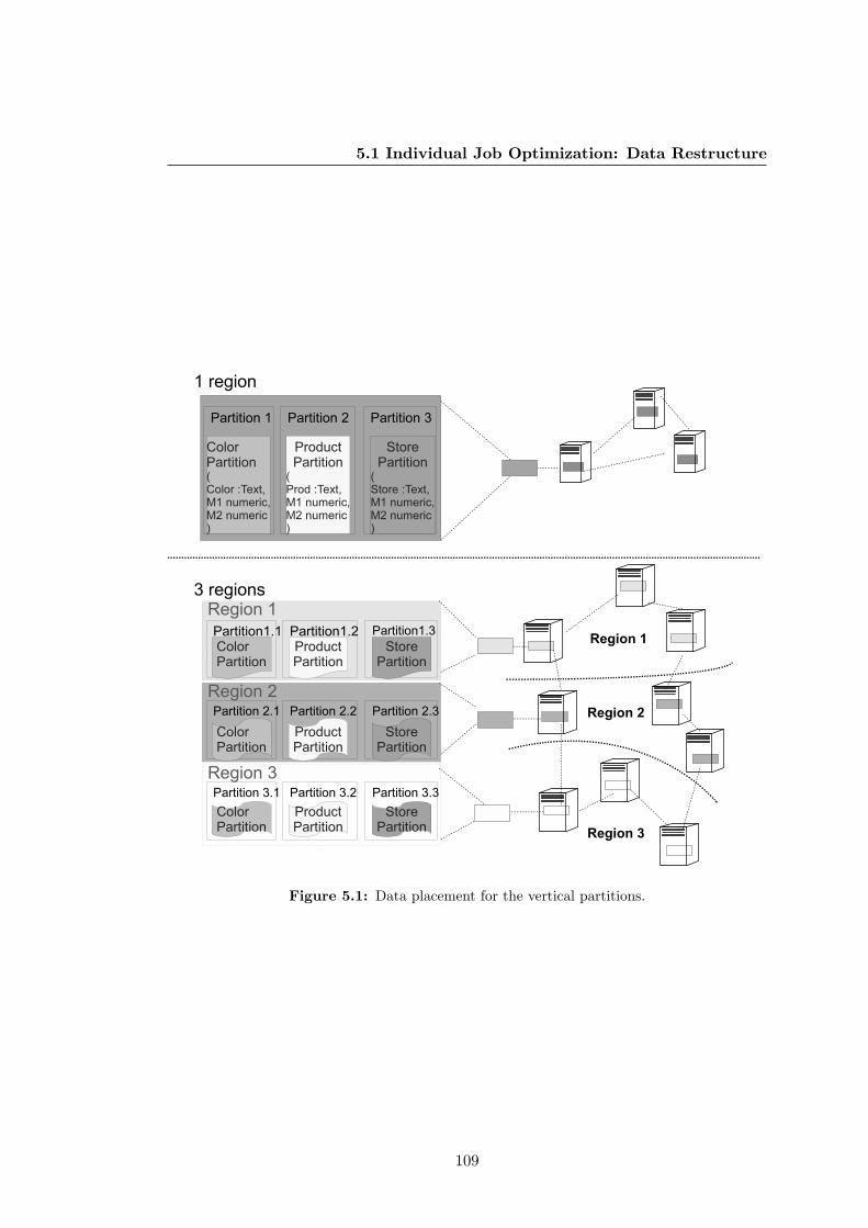
5.1 Individual Job Optimization: Data Restructure
Figure 5.1: Data placement for the vertical partitions.
109

5. PERFORMANCE IMPROVEMENT
this circumstance, the inverted indexing technique is more suitable, since its special
structure allows for retrieving data in a batch fashion. Refer to Section 2.2.4 for details
on inverted index.
Inverted index was originally designed to handle unstructured data, such as data
contained in web pages. Apache Lucene (16) realized the inverted indexing technique.
The concepts used in Lucene are based on unstructured data. For example, in Lucene, a
Document is a collection of Fieldables; a Fieldable is a logical representation of a user’s
content that needs to be indexed or stored. In order to utilize Lucene to index structured
data, a record is considered as a Document of Lucene, and each column’s value of the
record is considered as a Fieldable. Thus, recordID corresponds DocumentID of Lucene.
When searching a keyword of a certain column in an inverted index, we get a set of
recordIDs with which associate the records containing this keyword.
5.1.2.2 Data Compressing
In this work, the data restructuring procedure does not only realize the Lucene-based
inverted indexation, but also realize a data compressing procedure. For the Dimensions,
the ”text” type distinct value is converted into an integer. We call this integer as the
code of the distinct value. Both of these integer values and float values of Measures are
compressed into bytes before written to the disk.
For each horizontal partition, the compressed data is stored in two files, FactIndex
and Fact. Fact file stores distinct values of each dimension and the measure values
contained in each record. These values are organized record by record in Fact file.
The FactIndex file stores a set of addresses. Each address pointing to the position
of each record stored in Fact file. Figure 5.2(a) shows the compressed data storage
for horizontal partitions. Similarly, for each vertical partition, the compressed data is
also stored in FactIndex and Fact. Instead of storing integer values for all dimensions,
only one integer value is stored for each record. The float values of all measures are
still stored for each record. Figure 5.2(b) shows the compressed data files for vertical
partitions.
110

5.1 Individual Job Optimization: Data Restructure
(a)
(b)
Figure 5.2: (a) Compressed data files for one horizontal partition. (b) Compressed datafiles for one vertical partition of dimension x. (DV means Distinct Value)
111
5. PERFORMANCE IMPROVEMENT
5.2 Mapper and Reducer Definitions
Processing a Multiple Group-by query consists of filtering and aggregating phases. Over
the restructured data, the computations involved in these two phases are different than
before. Instead of a raw data scanning, filtering phase performs a search operation
over inverted index with a keyword coming from the WHERE condition. Such a search
operation retrieves from inverted index a list of recordIDs, indicating the records satis-
fying the given condition. With the recordID list, the aggregating phase can locate the
selected records and compute aggregates by reading filtered data from their compressed
data file.
In the previous work, we learned that performing aggregating phase within combin-
ers could reduce execution time. Lately, we realized that aggregating phase could be
moved into mappers for purpose of reducing the size of the intermediate output from
mappers. As a result, we let mappers perform filtering and aggregating phases, and
reducer merges the aggregate tables from mappers and generates the final result.
Under different data partitioning methods, data organization is different, and the
job definitions are not the same. In our implementation under the horizontal partition-
ing, the mapper applies the WHERE condition and then aggregates for all dimensions
appearing in Group-by dimensions over each data partition. In our implementation
under the vertical partitioning, mapper performs the filtering operations, and then ag-
gregates for one dimension, since each vertical partition includes only one dimension.
We present the detailed Mapper and Reducer definition in the following content.
5.2.1 Under Horizontal Partitioning
Mapper
Under the horizontal partitioning, a mapper starts with the filtering phase. In filter-
ing phase, records are filtered with the WHERE condition through a ”search” operation
which looks for the given keyword within the Lucene index file (denoted as index). As
a result, a recordID list (denoted as slctRIDs) in type of BitSet (5) is produced. In
filtering phase, dimensions are also filtered. Only those dimensions appearing in the
Group-by clauses (denoted as GBDims) are selected.
After that, processing enters into the aggregating phase. Multiple aggregate tables
are created for selected dimensions (denoted as slctDims). These tables are initialized
112
5.2 Mapper and Reducer Definitions
with distinct values of corresponding dimension. We designed a new data structure of
aggregate table and enhanced its functionality. The basic functionality of new aggregate
table remains the same as in Chapter 4, which means storing for each Group-by di-
mension distinct values and the corresponding aggregate values for each distinct value.
Differently, the new structure can additionally record the aggregate function list given
in query, and it provides implementations for various aggregate functions, which al-
lows computing aggregate values by calling the built-in functions. Besides, the new
aggregate table structure stores the name of dimension.
Since in one mapper, aggregating phase only aggregates over one partition of the
entire ROWSET, the aggregate table only contains a partial of the aggregates, and we
mark the partial aggregate table as agg part. The text type distinct value of all the
selected dimensions, as well as the numeric values of all the measures in the selected
records is read from the compressed data (CD) file. The following computations are
performed each time one selected record is retrieved. Values of all Group-by dimensions
are read from the retrieved record. For every Group-by dimension, the aggregated
value associated with the read distinct value is updated by the measure values from
the retrieved record. It is necessary to distinguish two cases. In one case, the current
record is the first one that contributes to the aggregate values of one distinct value.
In this case, we compute the aggregates with newly arrived measure values, and insert
a new record with the computed aggregate values. Otherwise, the current record is
not the first contributing one, then recalculate aggregate values by aggregating the
existing aggregate values with newly arrived measure values, and update them. The
pseudo-code in Algorithm 3 describes this procedure.
Reducer
The reducer collects all the intermediate outputs, i.e. partial aggregate tables pro-
duced by mappers. Each mapper produces multiple aggregate tables, each aggregate
table for one Group-by dimension. One mapper processes aggregations over multiple
dimensions. If we mark the number of Group-by queries as nbGB, then each mapper
produces nbGB partial aggregate tables, noted as, agg part[nbGB]. Assuming that there
are, in total, nbm mappers, the number of intermediate aggregate tables is equal to the
product of the mapper number and the Group-by dimension number, i.e. nbm×nbGB.
The intermediate output from the same mapper is sent back in one message. Reducer
113
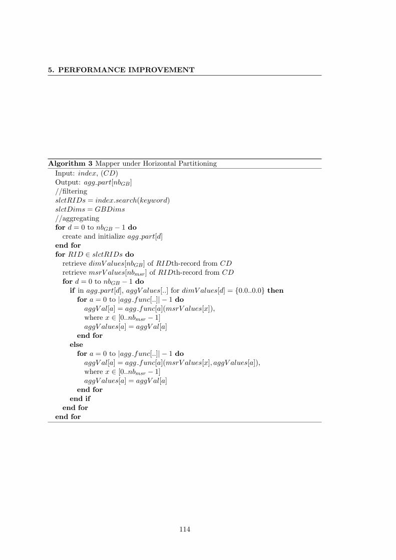
5. PERFORMANCE IMPROVEMENT
Algorithm 3 Mapper under Horizontal Partitioning
Input: index, (CD)Output: agg part[nbGB]//filteringslctRIDs = index.search(keyword)slctDims = GBDims//aggregatingfor d = 0 to nbGB − 1 do
create and initialize agg part[d]end forfor RID ∈ slctRIDs do
retrieve dimV alues[nbGB] of RIDth-record from CDretrieve msrV alues[nbmsr] of RIDth-record from CDfor d = 0 to nbGB − 1 do
if in agg part[d], aggV alues[..] for dimV alues[d] = {0.0..0.0} thenfor a = 0 to |agg func[..]| − 1 do
aggV al[a] = agg func[a](msrV alues[x]),where x ∈ [0..nbmsr − 1]aggV alues[a] = aggV al[a]
end forelse
for a = 0 to |agg func[..]| − 1 doaggV al[a] = agg func[a](msrV alues[x], aggV alues[a]),where x ∈ [0..nbmsr − 1]aggV alues[a] = aggV al[a]
end forend if
end forend for
114

5.2 Mapper and Reducer Definitions
processes the intermediate outputs mapper by mapper. After creating a set of empty
aggregate tables, denoted as agg[nbGB], then it calls the merge function to merge the
partial aggregate tables produced by each mapper with the initialized aggregate tables.
The pseudo-code in Algorithm 4 describes this processing procedure.
Algorithm 4 Reducer under Horizontal Partitioning
Input: mp output[nbm] < agg part[nbGB] > //nbm: mapper numberOutput: agg[nbGB]for g = 0 to nbGB − 1 do
create agg[g] //create the gth aggregate tableend forfor m = 0 to nbm − 1 do
agg part[..]← mp output[m]for g = 0 to nbGB − 1 do
merge agg part[g] with agg[g]end for
end for
5.2.2 Under Vertical Partitioning
Mapper
Under the vertical partitioning, the index and compressed data is organized partition
by partition. The processing a Group-by query actually involves data of two partitions,
since filtering with the WHERE condition needs to access one partition, aggregating
phase needs to access another partition. This is the usual case. It is uncommon that a
Group-by query aggregates over a dimension which appears in the WHERE condition.
In filtering phase, mapper applies condition by searching the given keyword within
Lucene index of the partition concerned by WHERE condition, and produces a selected
recordID-list. As mentioned above, the aggregating phase works on a different parti-
tion, which is the corresponding partition of the Group-by dimension. The selected
recordID-list is used to interactively retrieve dimension value and measure values from
the compressed data file. At the same time, the aggregate computations are performed.
When a record being retrieved, the aggregate functions are performed to calculate the
new aggregate values. The aggregate function either aggregates over the newly read
measure values and the existing aggregate values, or, if the current record is the first
115

5. PERFORMANCE IMPROVEMENT
contributor to the aggregate value of current distinct value, the aggregate function com-
pute the aggregate values only with the new measured values. The aggregate values
are updated into the aggregate table.
Note that, we use the same mapper computation both vertically partitioned data
and hybrid partitioned data. The only difference is in the generated intermediate ag-
gregate table. Mapper working over a complete vertical partition produces an complete
aggregate table. The aggregate table contains aggregate values for all distinct value.
It is not necessary to aggregate such an aggregate table with other aggregate tables to
generate the final result in reducer. On the contrary, the mapper working on a hybrid
partition can only produce a partial aggregate table. For generating the final result,
multiple partial aggregate tables need to be re-aggregated in reducer. This difference is
automatically managed in our program. In order to distinguish from the final aggregate
table, which is noted as agg, we still mark the output of mapper as agg part for both
cases. The detailed mapper pseudo-code is listed in Algorithm5.
Algorithm 5 Mapper under Vertical Partitioning
Input: index, CD, dim // CD: Compressed DataOutput: agg part//filtering phaseslctRIDs = index.search(keyword)//aggregating phasefor all RID ∈ slctRIDs do
retrieve dimV alue of RIDth-record from CD)retrieve msrV alues[nbmsr] of RIDth-record from CDif in agg part, aggV alues[..] for dimV alue = {0.0..0.0} then
for a = 0 to |agg func[..]| − 1 doaggV al[a] = agg func[a](msrV alues[x])where x ∈ [0..nbmsr − 1]aggV alues[a] = aggV al[a]
end forelse
for a = 0 to |agg func[..]| − 1 doaggV al[a] = agg func[a](msrV alues[x], aggV alues[a])where x ∈ [0..nbmsr − 1]aggV alues[a] = aggV al[a]
end forend if
end for
116
5.3 Data-locating Based Job-scheduling
Reducer
The reducer collects aggregate tables agg parts produced by all mappers. Under
vertical partitioning, the total number of intermediate aggregate tables is equal to
the number of mappers. That is much smaller comparing with the number of agg part
produced by mappers over horizontal partitions. At the beginning of reducer, we create
and initialize nbGB aggregate tables, which will be updated during the calculation and
”outputed” as the final result at the end of reducer. For each partial aggregate table,
we first identify the aggregate table agg[x] serving for the same dimension. Then we
merge the aggregate values within the partial aggregate table to the final aggregate
table.
As mentioned above, one mapper may produce a complete aggregate table or a
partial aggregate table. However, reducer handles them using the same computation.
If an aggregate table is complete, then there will be no other aggregate table, which
corresponds to the same dimension. Thus, no aggregate table will be merged with it.
This is achieved automatically. For a partial aggregate table, there are naturally other
partial aggregate tables be merged with it. The pseudo-code in Algorithm 6 describes
this procedure.
Algorithm 6 Reducer under Vertical Partitioning
Input: mp output[nbm] < agg part >where nbm is number of mappersOutput: agg[nbGB]for g = 0 to nbGB − 1 do
create agg[g]end forfor m = 0 to nbm − 1 do
identify the target agg[x], where agg[x]serves the same dimension as agg part[m]aggregate agg[x] with agg part[m]
end for
5.3 Data-locating Based Job-scheduling
GridGain is a Multiple-Map-One-Reduce framework. It provides an automatic job-
scheduling scheme, which assumes all nodes are equally suitable for executing job. Un-
117
5. PERFORMANCE IMPROVEMENT
fortunately, that is not the case of our work. We provide a data-locating job-scheduling
scheme. This scheme can be simply described as sending job to where its input data is.
5.3.1 Job-scheduling Implementation
Our job-scheduling implementation helps mapper to accurately locate data partition.
This is especially important in case of no existence of data redundancy. One wrong map-
ping will cause computational errors. With the data placement procedure performed
during data restructuring, this job-scheduling scheme is converted to a data location
issue. We utilize the user-definable attribute mechanism provided by GridGain to ad-
dress this issue. For example, we add a user-defined attribute ”fragment” into each
worker’s GridGain configuration, and attribute it a value representing the data parti-
tions’ identifiers that it holds. When the worker nodes’ GridGain instances are started,
the ”fragment” attribute is visible to the master node’s GridGain instance and the
other worker nodes’ GridGain instances. It is used to identify the right worker node.
In the case of horizontal partitioning, worker node identifiers (i.e. hostnames) are
utilized to locate data partitions. In this case, an equal number of partitions are placed
on each worker node. The partitions containing successive records are placed over
one worker node. That is, partitions are distributed on worker nodes in a sequential
order. Then, the identifier of worker node is used as the identifier of data partitions
that it holds. In this way, worker node identifiers are used to locate data partitions.
For example, assuming that ROWSET is horizontally divided into 10 partitions, these
partitions are placed over 5 worker nodes. Thus, worker node A holds partitions 1, 2;
worker node B holds partitions 3, 4, and so on. In this scenario, 10 mappers need to
be dispatched. As partitions 1 and 2 locate on worker node A, then mappers 1 and 2
are sent to worker node A. The rest of mappers are scheduled in the same way.
In case of vertical partitioning, a user-defined attribute, ”region identifier” is utilized
to locate data partitions. When worker node number is small (case of 1 region), vertical
partitions are replicated across all worker nodes. When worker node number is large,
further, vertical partitions are horizontally divided into regions. Worker nodes are
accordingly re-organized into regions. The worker nodes of the same region have the
same ”region identifier”. Partitions are replicated across worker nodes within the same
region. Thus, the region identifiers of worker nodes are utilized for data partitions.
As an example, 13 vertical partitions from ROWSET having 10 000 000 records, are
118

5.3 Data-locating Based Job-scheduling
horizontally divided into 2 regions. The records 1 to 5 000 000 are put in region 1, and
the records 5 000 001 to 10 000 000 are put in region 2. 10 worker nodes are accordingly
re-organized into 2 regions, each containing 5 worker nodes. 10 mappers aggregate over
5 different dimensions in two different regions respectively. For load balancing reason,
we use round-robin policy within region to keep the job number running over each
worker as balanced as possible.
5.3.2 Discussion on Two-level Scheduling
We actually realize a two-level scheduling in MapReduce computations, i.e. task-level
scheduling and job-level scheduling. Task-level scheduling means dispatching each map-
per to the corresponding worker node. It considers how to distribute mappers, and
ignores the calculation details within each job (mapper). Several elements should be
considered in the task-level scheduling, such as mapper number, worker node number,
load balancing. In order to achieve load balancing, it is necessary to take into account
worker node’s performance and status, and the input data location, etc. As one job is
run on one worker node, job-level scheduling takes place within a worker node, since
one job runs on one worker node. Job-level scheduling considers the organization of
calculations within a mapper. The main calculations can be encapsulated into reusable
classes, and stored in a local jar file on each worker. Mapper calls the methods of these
classes to run those calculations. Job-level scheduling is closely related to calculations
that a job should execute. For this reason, the job-level scheduling should be tuned
according to different queries; on the contrary, the task-level scheduling could be un-
changed or slightly changed for different queries. Our mapper job definitions can be
considered as a job-level scheduling.
5.3.3 Alternative Job-scheduling Scheme
An alternative job-scheduling scheme is to perform filtering phase on the master node
and aggregating phase over worker nodes. This job-scheduling scheme is feasible since
the restructured data allows loosely coupled computations. In the preceding imple-
mentation, filtering phase and aggregating phase are not separable, since aggregating
phase computations consume filtering computations’ output. With restructured data,
we can see that the computations of these two phases are clearly decoupled, since they
use different files as input data. In filtering phase, a search operation is performed via
119

5. PERFORMANCE IMPROVEMENT
accessing only inverted index files (Lucene generated files). In aggregating phase, ag-
gregation is performed over filtered records identified by a list of recordID calculated by
filtering phase, and it only needs to accesses the compressed data files (FactIndex and
Fact files). As these two phases are decoupled, they can be scheduled and optimized
separately, which provides more flexibility for job-scheduling. This is especially helpful
in case of vertical partitioning, where the selected recordIDs is commonly usable for
multiple dimensions’ aggregations.
5.4 Speed-up Measurements
We evaluated our MapReduce-based Multiple Group-by query over restructured data in
a cluster of Grid’5000 located in Orsay site1. Also, we use the version of GridGain 2.1.1
over Java 1.6.0. The JVM’s maximum of heap size is set to 1536MB on both master
node and worker nodes. We ran our applications over 1 to 15 nodes. Although the
worker nodes were small-scaled, the ROWSET processed in these experiments is not
extremely large, and it fits well with the amount of nodes used in our work. ROWSET
was composed of 10 000 000 records with each including 15 columns. The size of
ROWSET was 1.2 GB. We partition the data set with both horizontal partitioning
and vertical partitioning. All the partitions had already been indexed with Lucene and
compressed before launching the experiments.
We chose queries having different selectivity. Selectivity is a factor that controls
the amount of data being processed in the aggregating phase. Four Multiple Group-by
queries’ selectivities are 1.06%, 9.9%, 18.5% and 43.1% respectively. These queries all
had the same five Group-by dimensions. Before starting the parallel experiments, we
ran a group of sequential versions for each of these queries and measured the execution
times, which were used as the baseline of the speed-up comparison.
5.4.1 Under Horizontal Partitioning
Under the horizontal partitioning, we partitioned the ROWSET with different sizes.
We ran concurrently different number of mappers over each worker node in different
experiments. Thus, we could compare the performance of running a few of big-grained
1The cluster located in Sophia site had unfortunately retired after doing our first part of experi-ments. The currently chosen cluster has the same hardware configuration as retired cluster of Sophia.
120
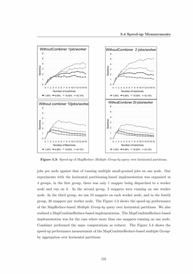
5.4 Speed-up Measurements
Figure 5.3: Speed-up of MapReduce Multiple Group-by query over horizontal partitions.
jobs per node against that of running multiple small-grained jobs on one node. Our
experiments with the horizontal partitioning-based implementation was organized in
4 groups, in the first group, there was only 1 mapper being dispatched to a worker
node and run on it. In the second group, 2 mappers were running on one worker
node. In the third group, we ran 10 mappers on each worker node, and in the fourth
group, 20 mappers per worker node. The Figure 5.3 shows the speed-up performance
of the MapReduce-based Multiple Group-by query over horizontal partitions. We also
realized a MapCombineReduce-based implementation. The MapCombineReduce-based
implementation was for the case where more than one mappers running on one node.
Combiner performed the same computations as reducer. The Figure 5.4 shows the
speed-up performance measurement of the MapCombineReduce-based multiple Group-
by aggregation over horizontal partitions.
121

5. PERFORMANCE IMPROVEMENT
Figure 5.4: Speed-up of MapCombineReduce Multiple Group-by query over horizontalpartitions.
122
5.4 Speed-up Measurements
Observation and Comparison
For the MapReduce-based implementation, the first observation of the speed-up mea-
surement is that the queries with big selectivity shows better speed-up performance
than the queries with small selectivity. A query with certain selectivity has a fixed
workload of calculation. Some parts of this workload are parallelizable, but others are
not. The reason why the big selectivity queries have better speed-up performance is
the parallelizable portion in their workload is greater than that in the small selectivity
queries. The second observation is the speed-up performances of smaller job number
per node (1 and 2 jobs/node) experiments surpass that of bigger job number per node
(10 and 20 jobs/node) experiments. Multiple jobs concurrently running over one node
were considered to be able to more efficiently utilize the CPU cycles, and can run
faster. But in reality, this is not always true. We will discuss the issue of multiple jobs
concurrently running on one worker node later in this chapter.
The speed-up of MapCombineReduce-based implementation is similar to that of
MapReduce-based one. Comparing these two implementations, we can see that the
speed-up performance of MapReduce-based implementation is better than that of MapCombineReduce-
based one in the experiments of small job number per node. In contrast, for experiments
of big job number per node, the MapCombineReduce-based implementation speeds up
better than MapReduce-based one. That is due to the necessity of combiner for dif-
ferent job number per node. For the job number per node smaller or around the CPU
number per node (e.g. 1 and 2), the pre-final-aggregation (combiner’s work) is not
necessary, in that the number of intermediate outputs is not big. On the contrary,
when the number of job per node is big (e.g. 10 and 20), the combiner is necessary. In
this case, the speed-up of MapCombineReduce-based implementation is slightly better
than the MapReduce-based implementation.
5.4.2 Under Vertical Partitioning
Under vertical partitioning, we dispatched the vertical partitions using the policies
described in Section 5.1.1.3. Similarly, we realized a MapReduce based implementation
and MapCombineReduce based one. We measured the speed-up performance for both
of them. During the experiments, we increased the number of worker nodes from 1 to 15,
and divided the experiments into 3 groups. In experiments of group 1, we had a small
worker node number, denoted as w, w ∈ [1..5], we organized vertical partitions into
123

5. PERFORMANCE IMPROVEMENT
one region. If we note region number as nbr, then nbr = 1. In this case, each mapper
aggregates over one entire Group-by dimension. Thus, then in case of 1 region, the
number of mappers is equal to the number of Group-by dimensions (nbm = nbGB = 5).
In the second group of experiments, we increased the number of region to two (nbr = 2)
in order to utilize till 10 worker nodes. We ran the queries over 2, 4, 6, 8 then 10 worker
nodes (i.e. w ∈ [2, 4, 6, 8, 10]), and measured the execution time in case of each vertical
partition being cut into two regions. As the number of mapper equals to the number
of partitions, then we have nbm = nbGB · nbr = 10. In the third group of experiments,
we increased the number of region to three, i.e. nbr = 3. We had worker nodes number
w ∈ [3, 6, 9, 12, 15] in different experiments. The number of mapper nbm = 15. The
mappers were evenly distributed within each region.
As we fixed the Group-by dimension number as 5, the total mapper number was
5×nbr, and the number of mappers per node was varying with node number per region:
nbjob/node =⌊
5/nbnode/region
⌋
or⌈
5/nbnode/region
⌉
For example, if nbnode = 1, nbr = 1,
then each node was assigned 5 mappers; if nbnode = 10, nbr = 2, then each node is
assigned 1 mapper; if nbnode = 2, nbr = 1, then one node was assigned 2 mappers, the
other 3 mappers, etc. We illustrate the speed-up performance measurements in the
Figure 5.5.
Observation and Comparison
As shown in this figure, the speed-up is increasing with the raise of worker number
regardless of the number of regions. The MapReduce-based implementation speeds up
better than the MapCombineReduce-based one, because the number of job per node is
small (i.e. < 5). The queries with bigger selectivity, like, 9.9%, 18.5%, 43.1%, benefit
more from the parallelization than the queries with smaller selectivity, like 1.06%.
For most of queries, the biggest speed-up appears in the third group of experiments
with 3 regions, for both the implementations MapReduce-based one and MapCombineReduce-
based one. Comparing the speed-up under vertical partitioning and that under the
horizontal partitioning, we can see the best speed-up appears in experiments under the
vertical partitioning. Under vertical partitioning, each mapper aggregates over only one
dimension; the obtained intermediate output is the aggregates of one dimension. The
size of the intermediate outputs with using vertical partitioning is much smaller than
those with using the horizontal partitioning. Imagining a scenario where 10 worker
124

5.4 Speed-up Measurements
Figure 5.5: Speed-up of MapReduce Multiple Group-by aggregation over vertical par-titions, MapReduce-based implementation is on the left side. MapCombineReduce-basedimplementation is on the right side.
125

5. PERFORMANCE IMPROVEMENT
nodes are available. Under horizontal partitioning, one mapper works on one horizon-
tal partition on one worker node. As each mapper aggregates over 5 dimensions, then,
the number of intermediate aggregate tables from all the mappers are 10 × 5 = 50.
Under vertical partitioning, 10 available workers are organized into 2 regions. Also,
there are in total 10 mappers. But each mapper aggregates over one dimension. Thus
the number of intermediate aggregate tables is exactly the number of mappers 10. If
we simply suppose that an aggregate table of an arbitrary Group-by dimension is of
size 20K, then 1000K intermediate output is generated under horizontal partitioning,
while 200K intermediate output is generated under vertical partitioning. Thus, with
vertical partitioning, the intermediate data volume to be transferred is reduced with
regard to the experiments with the horizontal partitioning.
5.5 Performance Affecting Factors
In this section, we will discover the performance affecting factors in the Multiple Group-
by query processing. Some of them are concerning the computations themselves, others
are related to the exterior condition, such as hardware, network, etc. Discovering of
these factors is helpful for locating the bottlenecks, and in turn increasing the system
efficiency. The performance affecting factors addressed in this section include, query
selectivity, running multiple jobs over one worker node, hitting data distribution, in-
termediate output size, serialization algorithms, network status, combiner’s utilization
as well as data partitioning methods.
5.5.1 Query Selectivity
Query selectivity is a factor that controls the records filtered out during the selecting
phase. Also, it determines the amount of data that the aggregating phase should
process. For big selectivity, query’s aggregating phase takes up a majority of the
whole calculation. In addition, the aggregating calculation is parallelizable. Thus
the query with big selectivity benefits more from the parallelization than query with
small selectivity. Query selectivity sometimes is related with workload skew. In some
particular cases a query selects a lot of records from some partitions, but very limited
records from the other partitions. Therefore, most aggregate operations are performed
only on a part of worker nodes, while the other nodes keep idle, which causes the
126
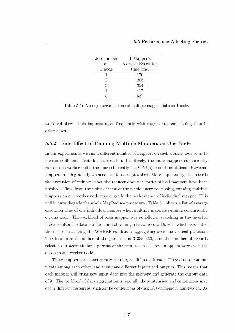
5.5 Performance Affecting Factors
Job number 1 Mapper’son Average Execution
1 node time (ms)
1 1702 2083 3544 4175 537
Table 5.1: Average execution time of multiple mappers jobs on 1 node.
workload skew. This happens more frequently with range data partitioning than in
other cases.
5.5.2 Side Effect of Running Multiple Mappers on One Node
In our experiments, we ran a different number of mappers on each worker node so as to
measure different effects for acceleration. Intuitively, the more mappers concurrently
run on one worker node, the more efficiently the CPU(s) should be utilized. However,
mappers run degradedly when contentions are provoked. More importantly, this retards
the execution of reducer, since the reducer does not start until all mappers have been
finished. Thus, from the point of view of the whole query processing, running multiple
mappers on one worker node may degrade the performance of individual mapper. This
will in turn degrade the whole MapReduce procedure. Table 5.1 shows a list of average
execution time of one individual mapper when multiple mappers running concurrently
on one node. The workload of each mapper was as follows: searching in the inverted
index to filter the data partition and obtaining a list of recordIDs with which associated
the records satisfying the WHERE condition; aggregating over one vertical partition.
The total record number of the partition is 3 333 333, and the number of records
selected out accounts for 1 percent of the total records. These mappers were executed
on one same worker node.
These mappers are concurrently running as different threads. They do not commu-
nicate among each other, and they have different inputs and outputs. This means that
each mapper will bring new input data into the memory and generate the output data
of it. The workload of data aggregation is typically data-intensive, and contentions may
occur different resources, such as the contentions of disk I/O or memory bandwidth. As
127

5. PERFORMANCE IMPROVEMENT
shown in this table, when running only one mapper over one worker node, the execu-
tion time is relatively small (170 ms). When concurrently running 2 mappers over one
worker node, the average execution time of one individual mapper is lightly dragged (37
ms longer). When concurrently running 3 or more mappers over one worker node, the
execution time shows a relatively large delay (from 184 ms to 367 ms). We can see that,
on one worker node with 2 CPUs, having 2 concurrently running mappers, the average
execution time is the most interesting. After that, when we continuously increased the
number of mappers on the worker node, the more mappers were concurrently running
on one worker node, the longer time an individual mapper takes.
5.5.3 Hitting Data Distribution
The data intensive application involves a large number of data read operations. The
execution time is affected by the hitting data’s distribution. By hitting data, we mean
the data item that a read operation is going to locate and read. The hitting data’s
distribution means the distribution of all the hitting data items’ storage positions in
one file. If the distribution of hitting data items is concentrated, then less operations of
disk I/O are invoked. Otherwise, if the distribution of hitting data items is dispersed,
then more operations of disk I/O are invoked.
This is a result of using the buffering technique, which is widely used to realize read
operations. Buffering technique can help to reduce the number of disk I/O operations.
Buffer is actually a region in memory of a given size, for example, 1024 Bytes. The data
stored in the buffer is fetched within one disk read operation. When a read operation
with a given file read position is invoked, it will first check whether the data item
of the give position is already loaded into the buffer. If that is the case, then the
read operation will directly read the data item from the buffer. If the given file read
position is exceeded the data scope held in buffer, then a buffer refill operation will be
invoked. Thus, a disk read operation is caused. It seeks in the file stored on disk and
then continuously fetches data items from this position to the buffer, until the buffer
is filled.
In the processing of Multiple Group-by query, the computations in aggregating phase
involves reading data of each selected records. The selected records distribution in
stored file becomes a factor that affects the execution time. This is relatively more
obvious in the experiments using horizontal data partitioning than in the experiments
128

5.5 Performance Affecting Factors
(a)
(b)
Figure 5.6: Hitting data distribution: (a) Hitting data distribution of qurey with WHEREcondition ”Color=’Pink’ ”(selectivity=1.06%) in the first 2000 records of ROWSET; (b)Hitting data distribution of query with WHERE condition ”Product Family=’Accessories’”(selectivity=43.1%) in the first 2000 records of ROWSET.
using vertical partitioning. Taking an example in our work, in order to do aggregation,
we aggregated over various Group-by dimensions after read each selected record. Re-
garding the execution time, the worst case appeared in our experiments is the query
with the WHERE condition of ”Color=’Pink’”(selectivity=1.06%). In this case, hitting
data items are very dispersed, and the average time for aggregating one record is 5500
nanoseconds. On the contrary, for the query with WHERE condition ”Product Fam-
ily=’Accessories’ ”(selectivity=43.1%), the average time for aggregating one selected
records is 1000 nanoseconds. In order to be more illustrative, we visualize the distribu-
tion of hitting data of these two cases in Figure 5.6. The axis x represents the recordID,
and a vertical black line represents that the record hits the WHERE condition. We
visualize only the first 2000 records in these figures.
A simple calculation can make this clearer. In the compressed data file, we stored
for each record the compressed dimension values, and measure values. In our case of
horizontal partitioning, one record is composed of 13 dimension values of ”text” type,
and 2 measure values of float type. Under the compressed data format, one dimension
value is first replaced by an integer and then converted into 1 byte data; one float
measure value is converted into 4 bytes data. Thus, one record is converted into 21
bytes (13×1 bytes + 2×4 bytes = 21 bytes) in the compressed format. A buffer of 1024
bytes is capable of accommodating 1024÷21 ≈ 49 records. In case of the sub-figure (a),
where 1.06% records are selected, and the hitting data distribution is very dispersed.
129

5. PERFORMANCE IMPROVEMENT
In this case, one buffer refill (i.e. disk read operation) is caused for processing each
selected record. In case of the sub-figure (b) 43.1% records are selected. The hitting
data distribution is rather concentrated, there even exists a lot of selected records
that are contiguously stored. In this extreme case (continuous storage), processing 21
selected records will only cause one buffer refill. Disk read is one of the most expensive
operations. That explains the big difference of the average per record processing time
between these two cases. The similar case also occurred in the filtering phase. We
observed a various difference among the average time for retrieving one recordID of
selected records when processing queries with different selectivities.
5.5.4 Intermediate Output Size
Except for the overhead for computing the aggregates, the cost for transferring inter-
mediate output is also an overhead that we cannot ignore. Without considering the
uncontrollable factor of available network bandwidth, the main factor controlling this
overhead is the size of intermediate output. In our work, distinct value number of each
Group-by dimension, aggregate function number, mapper number and data partitioning
method affect the size of intermediate aggregate tables.
Distinct value number of one dimension and aggregate function number determines
the size of current dimensions aggregate table. The distinct value number of a certain
dimension determines the number of rows composing the corresponding aggregate table.
Each row stores the aggregates values for one distinct value. The number of aggregate
functions determines the number of columns composing the aggregate table. In each
row, one cell stores distinct value, and for each aggregate function, one additional cell
is used for storing the data item calculated by the aggregate function. As a result, one
row stores 1 value of type integer plus |agg func[..]| values of type float.
While the first two factors determine the individual aggregate table size. Mapper
number and data partitioning method affect the total size of all the intermediate aggre-
gate tables. Under horizontal partitioning, each mapper produces multiple aggregate
tables, where the number of aggregate tables is the product of Group-by dimension
number (denoted as nbGB) and mapper number (denoted as nbm). Under vertical par-
titioning, each mapper produces one aggregate table for a particular dimension, and
the number of aggregate tables is the number of mappers. Similarly, under hybrid
partitioning, the number of aggregate tables is also the number of mappers.
130

5.5 Performance Affecting Factors
In practice, individual aggregate tables concerning to different dimensions have
different size. If we note the total number of distinct values for all the Group-by
dimensions (nbDV ), we can calculate the intermediate output size under horizontal
partitioning as follows: nbm×nbDV×nbGB×[sizeof(int)+sizeof(float)×|agg func[..]|]
Under vertical partitioning, the mapper number is closely correlated with the num-
ber of region number (nbr). A set of aggregate tables—each for a Group-by dimension—
are produced by one region’s mappers. Then we have the intermediate output size as:
nbr × nbDV × nbGB × [sizeof(int) + sizeof(float)× |agg func[..]|]
5.5.5 Serialization Algorithms
Serialization is a process for converting a data structure or an object into a sequence
of bytes so in order to transmit it across network and be restored to the original state.
De-serialization is the inverse process of serialization. They are crucial for distributed
applications. In our experiments, we noticed that a portion of time non-ignorable is
used to serialize and de-serialize the data being transferred. Sometimes, this portion
of time reaches 50% of the total execution time.
There exist various serialization algorithms. For example, some of them are designed
for message sending based applications, where objects are smaller and infrequently re-
peated; some others of them are designed for streaming protocol based applications,
where the objects are big and usually repeated. Some algorithms are time-efficient; oth-
ers are space-efficient. Also, a serialization can either be performed during runtime or
during the compile-time (89). GridGain provides three alternatives of serialization/de-
serialization, one is based on JBoss serialization, one is based on JDK serialization, and
the other is based on XStream1. We adopted JBoss serialization based one, since it is
the default choice and the most time-efficient one among them.
Regarding the size of serialized object, the serialized object size is usually larger
than the original object. A serialized object needs contain sufficient information to
restore the original object. The class description of current object and its supper-class
description, as well as the other serializable objects referenced by current object should
be included in the generated serialized object. As a result, the serialized object is larger
than its original object. There exist some work trying to reduce the size of serialized
object, like in (81).
1XStream is a library to serialize objects to XML and back again.
131
5. PERFORMANCE IMPROVEMENT
In our work, two types of data are serialized and transmitted, i.e., mapper objects
and aggregate tables. The serialization of mapper objects happens during the start-
up phase of a MapReduce task. The mappers are sequentially serialized one after
another on the master node. The serialization for the first instance of mapper class
takes much longer time than the following instances of the same mapper class. The
aggregate tables are also sequentially de-serialized when they arrived at the master
node. The de-serialization times for aggregate tables are varying, and we did not
observe regularity over their changes. Over the worker nodes, we observed a small
overhead for de-serializing the mapper instance, but a non-ignorable serialization time
for aggregate tables.
Taking a close look at the two main types of transmitted data, we find that map-
per object and aggregate tables are of different type. Mapper object has a complex
structure, being composed of many super classes, references and parameters. This will
cause a big overhead for rewriting the class descriptions. Fortunately, in our case,
the serialization process is repeated multiple times within one process, for serializing
mapper objects with different status, which make it possible to do optimization. In
contrast, aggregate table’s structure is relatively simple, but contains big size of data.
The data types are mostly primitive, like integers and floats. Therefore, the desirable
serialization/de-serialization algorithms for our application need to be compatible to
both types of data. The future work will address this issue.
5.5.6 Other Factors
Except for the above performance affecting factors, there exist some other factors, such
as network status, utilization of combiner, and data partitioning methods. We have
already discussed them is earlier work, here we only want to give a short summary for
them.
Network status
Network status together with the size of serialized objects determines the execution
time of data transmission. It involves not only the available bandwidth over network,
but also the physical location of two communicating components. The data transfer
takes longer time if two communicating components are located in different clusters
than if they are within the same cluster. In our experiments, we adopted a single
132

5.6 Cost Estimation Model
cluster, where the network bandwidth is stable. By observation, the execution times
for sending mapper objects did not significantly change1.
Use or not Combiner
Using combiner component reduces a lot the execution time in the work of Chapter
4. In this previous work, we ran a relatively large number of mappers over one worker
node. Also, the intermediate output’s data structure (i.e. aggregate table) was not
compact. However, combiner component’s utilization is not always favorable. As we
can see in the resent work, the combiner component’s utilization did not significantly
reduce the execution time. On the contrary, it caused more overheads in certain cases.
In case where the number of mappers over one worker node is small, it is not neces-
sary to use the combiner component. However, our MapCombineReduce construction
using two successive MapReduce tasks is still significant, since it allows executing a
MapCombineReduce job in GridGain.
Data partitioning methods
In our work, the data partitioning methods determines multiple issues concerning
the execution of mappers and reducer. Firstly, it determines the index creation and
data compressing in data restructure phase. It, in turn, determines the computations
performed during MapReduce procedure. Finally, it determines the size of intermediate
output.
5.6 Cost Estimation Model
In this section, we give a cost estimation model for the execution time during the whole
MapReduce-based query processing on the restructured data. For the sake of time
limitation, we worked only on the cost estimation for the MapReduced-based imple-
mentation, and the cost estimation for MapCombineReduce-based implementation is
not addressed in this work. The above-mentioned performance effecting factors and
observation based on our experiments are maximally considered for constructing the
cost estimation model.
1The size of mapper is constant. For this reason, we use it to observe execution time changes
133
5. PERFORMANCE IMPROVEMENT
We still consider the four parts of cost in a MapReduce procedure, start-up, map-
per’s execution, closure and communication. In start-up, the master prepares the
mappers, including mapping mappers to available worker nodes, then serializing map-
per objects. The serialization for the first mapper object takes longer time than the
serializations for the other mapper objects. The formal cost estimation for start-up is
as follows:
Cst = Cmpg · nbm + Cs · sizem + C ′
s · (nbm − 1) · sizem
If there is no additional specification, the notations used in the formulas of this
chapter can be referred in Table 4.1. In above formula, we estimate the cost for com-
puting the mappings as Cmpg ·nbm, the serialization time for the first mapper object as
Cs · sizem, the serialization time for the rest of mapper objects as Cs · (nbm− 1) · sizem
When a worker receives a message of mapper, it de-serializes the mapper object,
then executes mapper job. When finished, it serializes aggregate table produced by
mapper. Taking into account the factor of running multiple mappers on one worker
node, we add a function of mapper number per node (denoted as f(nbm/node)) into the
estimation. Thus, the execution time of this process is estimated as:
Cw = f(nbm/node) · (Cd · γ · sizem + Cm + Cs · sizeagg)
Here, γ · sizem, (γ > 1) is used to represent the size of serialized mapper object. A
serialized object is always bigger than the original one, so, we have γ > 1. Also, γ is
varying according to the composition of object. The notation sizeagg means the size
of generated aggregate table. The mapper execution cost Cm and aggregate table size
sizeagg are varying according to the adopted partitioning methods. We will respectively
give the detailed estimations for the horizontal partitioning-based implementation and
the vertical partitioning-based one lately.
The closure includes de-serialization of the intermediate aggregate tables and user-
defined reducer’s execution. We estimate the closure cost as below:
Ccl = Cd ·
nbm∑
i=1
γ · sizeagg i + Cr
134

5.6 Cost Estimation Model
where the reducer cost (denoted as Cr) is varying with different applications. We will
give the estimation of reducer lately.
In our work, the data communication is composed of master node sending mappers
to the worker nodes, and worker nodes sending intermediate aggregate tables to master
node. Considering the size of transmitted data and the network status we estimate the
communication cost as:
Ccmm = Cn · (nbm · γ · sizem +
nbm∑
i=1
γ · sizeagg i)
where sizeagg i represents the size of the ith aggregate table produced by mappers.
5.6.1 Cost Estimation of Implementation over Horizontal Partitions
For the implementation over horizontal partitions, the mapper takes a horizontal par-
tition as input data, searches in its Lucene index, read values of dimensions and ag-
gregates with measures over the distinct values of Group-by dimensions. We assume
there exist D dimensions and M measures in ROWSET, over which we run the query
aggregating on nbGB Group-by dimensions. The mapper cost is estimated as below:
Cm = S ·N
nbm· {α · Cf + β · (nbGB + 4M) · Crd + nbagg · nbGB · Ca}
where Cf estimates the average execution time for successfully obtaining one recor-
dID of the selected records by searching Lucene index; Crd represents the execution
time for retrieve 1 byte from compressed file; nbagg means the number of aggregate
functions defined in the query. A distinct value is represented as an integer (i.e. dis-
tinct value code) of size 1 byte1, and a measure value as a float sized 4 bytes. As
mentioned before, record filtering and record reading operations are impacted by hit-
ting data distribution issue, which means, the average time for processing one unit of
data is varying with query selectivity. Therefore, two parameters α and β are applied
over the corresponding items. Their values are varying with different queries.
Under horizontal partitioning, each mapper produces aggregate tables for all Group-
by dimensions. The size of aggregate table can be estimated as follows:
1In our work, distinct value number of any dimension is smaller than 256, thus, 1 byte is sufficientto represent all distinct value code in integer of any dimension.
135

5. PERFORMANCE IMPROVEMENT
sizeagg =
nbGB∑
i=1
nbDVi· (1 + 4nbagg)
where nbDVirepresents the number of distinct values of the ith Group-by dimension.
1 + 4nbagg is the number of bytes containing in one row of aggregate table.
As the reducer takes all intermediate outputs of mappers as input and performs
aggregation over them, we estimate cost of reducer as:
Cr = Ca · nbagg · nbm ·
nbGB∑
i=1
nbDVi(1)
With these detailed estimation, we ignore the function f(nbm/node), since we address
on the small job per node cases, which is the most common case. Thus, we obtain the
total execution time estimation of the horizontal partitioning-based Multiple Group-by
query as below:
Costhp = Cmpg · nbm + Cs · sizem + C ′
s · (nbm − 1) · sizem + Cd · γ · sizem+
S ·N
nbm
· [α · Cf + β · (nbGB + 4M) · Crd + nbagg · nbGB · Ca] + Cs ·
nbGB∑
i=1
nbDVi· (1 + 4nbagg)+
Cd·nbm·
nbGB∑
i=1
nbDVi·(1+4nbagg)+Ca·nbagg·nbm
nbGB∑
i=1
nbDVi+Cn·nbm·γ·sizem+Cn·γ·
nbm∑
i=1
sizeSaggi
If we note the average size of serialized aggregate table as γ·∑nbGB
i=1 nbDVi·1 + 4nbagg.
We estimate the value of parameters as described in table 5.2. As it is difficult to accu-
rately estimate the serialization/de-serialization execution time for a unit of data, we
estimate the serialization/de-serialization time for the really used data in our exper-
iments. Therefore, the estimation values for these parameters are accompanied with
the size of data being serialized or de-serialized.
In order to test the accuracy of our execution time estimation model, we compare
the speed-up curve calculated from our model to the measured speed-up curve. The
Figure 5.7 are two speed-up curves for MapReduce based query processing on horizontal
partitions, with the number of worker nodes gradually increasing from 1 to 15. We chose
the case where only one mapper concurrently running on a worker node. In this case,
the application related parameter can be determined, such as, total record number
136
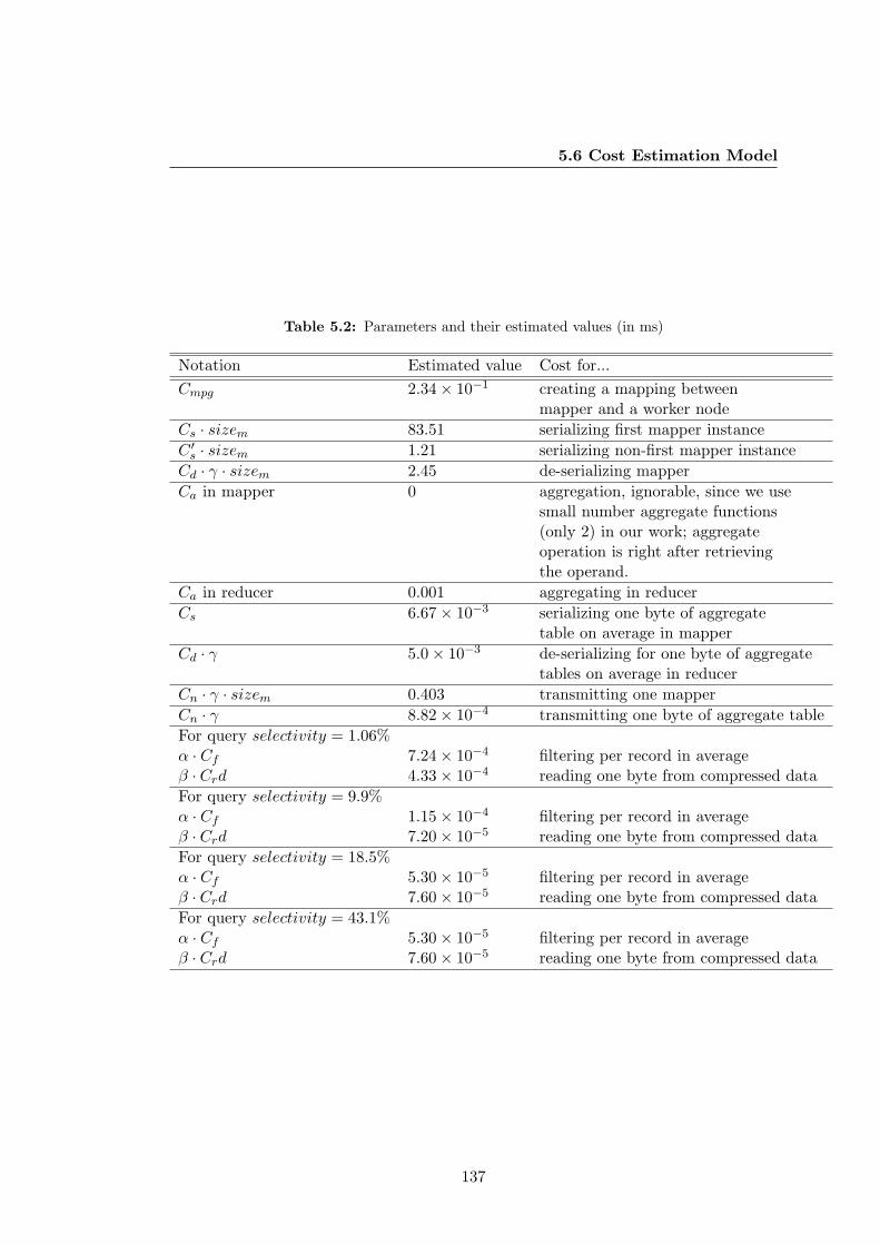
5.6 Cost Estimation Model
Table 5.2: Parameters and their estimated values (in ms)
Notation Estimated value Cost for...
Cmpg 2.34× 10⁻¹ creating a mapping betweenmapper and a worker node
Cs · sizem 83.51 serializing first mapper instance
C ′
s · sizem 1.21 serializing non-first mapper instance
Cd · γ · sizem 2.45 de-serializing mapper
Ca in mapper 0 aggregation, ignorable, since we usesmall number aggregate functions(only 2) in our work; aggregateoperation is right after retrievingthe operand.
Ca in reducer 0.001 aggregating in reducer
Cs 6.67× 10⁻³ serializing one byte of aggregatetable on average in mapper
Cd · γ 5.0× 10⁻³ de-serializing for one byte of aggregatetables on average in reducer
Cn · γ · sizem 0.403 transmitting one mapper
Cn · γ 8.82× 10⁻⁴ transmitting one byte of aggregate table
For query selectivity = 1.06%α · Cf 7.24× 10⁻⁴ filtering per record in averageβ · Crd 4.33× 10⁻⁴ reading one byte from compressed data
For query selectivity = 9.9%α · Cf 1.15× 10⁻⁴ filtering per record in averageβ · Crd 7.20× 10⁻⁵ reading one byte from compressed data
For query selectivity = 18.5%α · Cf 5.30× 10⁻⁵ filtering per record in averageβ · Crd 7.60× 10⁻⁵ reading one byte from compressed data
For query selectivity = 43.1%α · Cf 5.30× 10⁻⁵ filtering per record in averageβ · Crd 7.60× 10⁻⁵ reading one byte from compressed data
137

5. PERFORMANCE IMPROVEMENT
Figure 5.7: Measured speedup curve vs. Modeled speedup curve for MapReduce basedquery on horizontal partitioned data, where the each work node runs one mapper.
N=10 000 000, aggregate function number nbagg = 2, total distinct values number∑nbGB
i=1 nbDVi= 511, Group-by dimension number nbGB = 5, measure values contained
in one record M = 2, etc.
5.6.2 Cost Estimation of Implementation over Vertical Partitions
We also estimate the cost of the implementation under the vertical partitioning in a
similar way. The mapper’s cost is estimated as:
Cm = S ·N
nbrgn· [Cf + (4M + 1) · Crd + Ca · nbagg]
where nbrgn means the number regions.
With vertical partitioning, each mapper aggregates over one dimension d then the
intermediate aggregate table size is estimated as:
sizeaggd= nbDVd
· (1 + 4nbagg)
where, nbnbDVdmeans the distinct value number of current Group-by dimension d;
(1 + 4nbagg) is the estimated size in byte of each row in aggregate table.
The reducer aggregates over a list of aggregate results; each of them is the aggregate
result of one dimension or a part of dimension in case of nbrgn > 1. The estimation of
138

5.6 Cost Estimation Model
the reducer is:
Cr = Ca · nbrgn · nbagg · γ ·
nbGB∑
i=1
nbDVi(2)
By summing up the above estimations, we obtain the total cost estimation of Mul-
tiple Group-by query processing over vertical partitions:
Costvp = Cmpg ·nbm+Cs·sizem+Cd·γ ·sizem+S ·N
nbrgn·[Cf +(4M+1)·Crd+nbagg ·Ca]+
Cs·nbDVd·(1+4nbagg)+Cd·γ ·nbrgn·
nbGB∑
i=1
nbDVi·(1+4nbagg)+Ca·nbrgn·nbagg
nbGB∑
i=1
nbDVi+
Cn · (nbm · γ · sizem + γ · nbrgn ·
nbGB∑
i=1
nbDVi· (1 + 4nbagg)
Here we replaced∑nbm
i=1 sizeaggiby nbrgn ·
∑nbGB
i=1 nbDVi·(1+4nbagg) since the partial
aggregate tables from different region effectively construct nbrgn times aggregates for
all Group-by dimensions. The same estimation for parameter values could also be done
for vertical partitioning base query processing. We will have this done in the future
work.
5.6.3 Comparison
Note that, for the same ROWSET partitioned horizontally and vertically, the number
of partitions in horizontal partitioning is larger than the number of regions in vertical
partitioning, that is, HP.nbpttn > V P.nbrgn. The reason is, in horizontal partitioning,
partition number is equal to mapper number, and we let mapper number equal to a
multiple of node number, so as to utilize all the available nodes. However, with vertical
partitioning, the region number is usually a sub-multiple of nodes number. Given
this established facts, HP.nbpttn > V P.nbrgn, we see that the reducer cost of vertical
partitioning-based implementation, which is expressed with formula (1), is smaller than
that of the horizontal partitioning-based one, which is expressed with formula (2). As
shown by the estimation, under both horizontal partitioning and vertical partitioning,
a great part of calculation is parallelized. We make the calculation reduced from scale
139
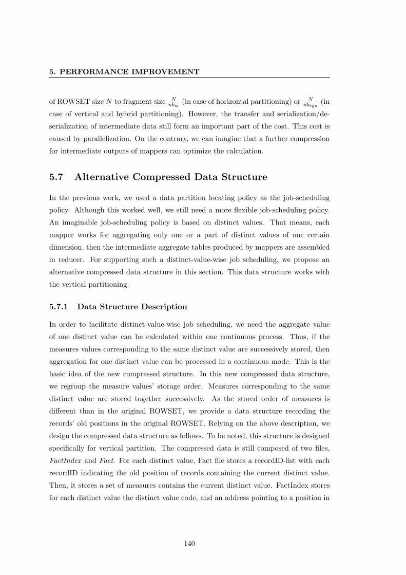
5. PERFORMANCE IMPROVEMENT
of ROWSET size N to fragment size Nnbm
(in case of horizontal partitioning) or Nnbrgn
(in
case of vertical and hybrid partitioning). However, the transfer and serialization/de-
serialization of intermediate data still form an important part of the cost. This cost is
caused by parallelization. On the contrary, we can imagine that a further compression
for intermediate outputs of mappers can optimize the calculation.
5.7 Alternative Compressed Data Structure
In the previous work, we used a data partition locating policy as the job-scheduling
policy. Although this worked well, we still need a more flexible job-scheduling policy.
An imaginable job-scheduling policy is based on distinct values. That means, each
mapper works for aggregating only one or a part of distinct values of one certain
dimension, then the intermediate aggregate tables produced by mappers are assembled
in reducer. For supporting such a distinct-value-wise job scheduling, we propose an
alternative compressed data structure in this section. This data structure works with
the vertical partitioning.
5.7.1 Data Structure Description
In order to facilitate distinct-value-wise job scheduling, we need the aggregate value
of one distinct value can be calculated within one continuous process. Thus, if the
measures values corresponding to the same distinct value are successively stored, then
aggregation for one distinct value can be processed in a continuous mode. This is the
basic idea of the new compressed structure. In this new compressed data structure,
we regroup the measure values’ storage order. Measures corresponding to the same
distinct value are stored together successively. As the stored order of measures is
different than in the original ROWSET, we provide a data structure recording the
records’ old positions in the original ROWSET. Relying on the above description, we
design the compressed data structure as follows. To be noted, this structure is designed
specifically for vertical partition. The compressed data is still composed of two files,
FactIndex and Fact. For each distinct value, Fact file stores a recordID-list with each
recordID indicating the old position of records containing the current distinct value.
Then, it stores a set of measures contains the current distinct value. FactIndex stores
for each distinct value the distinct value code, and an address pointing to a position in
140
5.7 Alternative Compressed Data Structure
Figure 5.8: Compressed data files suitable for distinct value level job scheduling withmeasures for each distinct value are stored together.
Fact file where the recordID-list and a set of measures covered by the current distinct
value start to store. Figure 5.8 illustrates this structure. For aggregating with using
this data structure, each mapper will be scheduled to aggregate over one distinct value.
FactIndex file is accessed to obtain the given distinct value’s storage position in Fact file.
Then, the mapper identifies the selected records covered by the given distinct values
by retrieving the common recordIDs of selected recordID-list from the filtering phase
and the recorID-list retrieved from Fact file. At last, the selected records covered by
the current value are aggregated using the measure values covered by current distinct
value retrieved from the Fact file.
5.7.2 Data Structures for Storing RecordID-list
Integer Array and Bitmap are two alternative data types can be used to store recordID
list. In case of using Integer Array, each recordID is stored as an element of the array.
In case of using Bitmap, we create a Bitmap being composed of a sequence of bits.
The number of bits is equal to the cardinality of the original ROWSET. One bit in
141
5. PERFORMANCE IMPROVEMENT
Bitmap corresponds one record. The value of each bit is either 0 or 1. If we use 1
to indicate that the current record’s id is in current distinct value’s recordID-list, we
obtain a Bitmap with all 1 positions indicating the whole recordID-list.
Considering the use of storage space, Integer Array and Bitmap are very different.
When the recordID-list contains a small number of elements, Integer Array takes smaller
storage spaces. In the opposite case, where the recordID-list contains a large number
of elements, Bitmap is more storage efficient.
5.7.3 Compressed Data Structures for Different Dimensions
Taking into account the above features, we distinguish two categories of dimensions:
dimensions having a small number of distinct values and dimensions having a large
number of distinct values. For those dimensions with a small number of distinct values,
then many records are covered by one certain distinct value. In turn, a large number
of recordIDs need to be stored. In this case, Bitmap is more space-saving and makes
access more efficient than Integer Array. For those dimensions with a large number of
distinct values, only a few recordIDs need to be stored. For this case, Integer Array
provides is more space-saving and provides more access efficiency.
But how to define the ”small” and ”large” over the number of distinct values for
one dimension? Let’s do a concrete calculation. Imagine that we have a ROWSET
containing 107 records. One recordID stored as integer takes 4 bytes. Assume that a
dimension includes V distinct values. Thus each distinct value covers 107/V records.
If we store the recordID-list in Integer Array, for one certain distinct value, 4× 10⁷/V
bytes are needed, on average. Then, we need to store 4×10⁷/V bytes in total in order to
store all recordIDs containing all distinct values. If we use a Bitmap to store recordID-
list of one distinct value, then the Bitmap takes 1.25×106 bytes. As a result, the critical
point of distinct value number V is 32. If V = 32, then two storage take the same space;
if V < 32, Bitmap takes smaller space; if DV > 32, then Integer Array takes smaller
space. Thus, if the number of distinct values is larger than 32, then we considered it as
”large”; otherwise, if the number of distinct value is smaller than or equal to 32, then
we consider it as ”small”. After defining the data structure of recordID-list, we specify
the concrete storage for those two dimensions. For dimensions having a large number
of distinct values, the composed data is composed of 2 files, FactIndex and Fact. Data
stored in the FactIndex file includes, the code of each distinct value of integer and an
142

5.7 Alternative Compressed Data Structure
Figure 5.9: Compressed data structure storing recordID list as Integer Array for dimen-sion with a large number of distinct values
address of long integer pointing to a position in the Fact file where the data related
to this distinct value is stored. Data stored in the Fact file includes three parts. The
first one is an integer representing the number of records covered by current distinct
value. The second one is an Integer Array compressed in Byte Array representing the
recordID-list for records covered by current distinct value. The third one is a Float
Array representing the measure values for records having the current distinct value.
Refer to Figure 5.9 for the illustration of this structure.
For dimension having small number of distinct values, the compressed data is also
composed of FactIndex file and Fact file. The FactIndex file stores the code of the
current distinct value in integer and an address in long integer, in long type, pointing
to a position in the Fact file where data related to this distinct value is stored. The
Fact file stores, for each distinct value, a Bitmap indicating the records covered by the
current distinct value, as a Byte Array, and the measure values for records having the
current distinct value in type of Float Array. Refer to Figure 5.10 for the illustration
of this structure.
143

5. PERFORMANCE IMPROVEMENT
Figure 5.10: Compressed data structure storing recordID list as Bitmap for dimensionwith a small number of distinct values (In Java, Bitmap is implemented as Bitset)
144

5.7 Alternative Compressed Data Structure
5.7.4 Measurements
We tested these two compressed data using a single machine, which is equipped with a 4-
core CPU running at 2.5GHz and 4 Go RAM. The objective is to measure the efficiency
provided by using these two different data structure over all dimensions. Table 5.3 shows
the execution time for four single Group-by queries having the following form:
SELECT group_by_dimension, SUM("quantity_sold"), SUM("revenue")
FROM "ROWSET"
WHERE condition
GROUP BY group_by_dimension
Those four single Group-by queries aggregates over dimensions, Product Family, Prod-
uct Category, Article Label and Store City, respectively. These four dimensions have
different distinct value number varying from 12 to 244. As shown in this table, the first
compressed data structure works well for aggregations over dimensions having large
number of distinct values and dimensions having small number of distinct values. For
the second compressed data structure, the aggregation over dimensions having small
number of distinct values is much faster than the aggregation over dimensions hav-
ing large number of distinct values. Even though, the aggregations over the second
compressed data are always slower than those over the first compressed data. The
compressed data using Bitmap did not provide the same efficiency as we imagined.
5.7.5 Bitmap Sparcity and Compressing
The low efficiency of Bitmap, i.e. the second compressed data used in above experi-
ments is caused by the sparcity. Even for a dimension having small number of distinct
values, for example, 12, the Bitmap is very sparse, since only 1/12 bits are set to
1. A Bitmap compressing is crucial for improving the storage efficiency. There exist
already some Bitmap compressing algorithms that we can take advantage of. These
methods typically employ Run-length-encoding, such as Byte-aligned Bitmap Code,
Word-Aligned Hybrid code and Position List Word Aligned Hybrid (4). Run-length-
encoding stores the sequence in which the same data value occurs in many consecutive
positions, namely run, as one single data value and count, instead of storing them as
the original run(19). We will address the Bitmap compressing methods in the future
work in order to improve our Bitmap’s storage efficiency.
145

5. PERFORMANCE IMPROVEMENT
RecordID list stored as Integer Array RecordID list stored as Bitmap
Group-by dimension Product Product Article Store Product Product Article StoreFamily Category Label City Family Category Label City
❳❳
❳❳
❳❳
❳❳
❳WHERE
DV nb
12 34 209 244 12 34 209 244
Color=Pink(S=1.06%) 547 500 516 453 968 1313 4219 3922
Product Family=Shirt Waist(S=9.9%) 469 453 438 437 562 797 3235 3812
Opening Year=2001(S=18.5%) 678 688 563 531 1031 1390 4344 3062
Product Family=Accessories(S=43.1%) 860 859 859 844 1079 1625 4203 4281
ALL(S=100%) 1844 1578 1531 1516 2344 2422 5484 5547
Table 5.3: Execution Times in ms of Group-by queries with different selectivities (S)using new compressed data structures. The numbers shown in italic represents that thecorresponding aggregations run over the dimensions correlated to the WHERE conditioninvolved dimension. For example, Product Family and Product Category are correlateddimensions.
5.8 Summary
In this work, we realized Multiple Group-by query on restructured data, using MapRe-
duce model to parallelize the calculation. We introduced the data partitioning, index-
ation and data compressing processing in data restructuring phase. The materialized
view ROWSET is partitioned respectively using two principal partitioning methods,
horizontal partitioning and vertical partitioning. The index that we created using
Lucene over ROWSET is an inverted index, which allows rapidly accessing and filter-
ing the records with WHERE condition. We measured our Multiple Group-by query
implementations over ROWSET, and compared the speed-up performance of implemen-
tations over horizontally partitioned data and that over vertically partitioned data. In
most cases, they showed similar speed-up performance, however, the best speed-up
appeared in the vertical partitioning-base implementation. Basing on the measured
result observations and analysis, we discovered several interesting factors that affect
query processing performance, including query selectivity, concurrently running map-
per number on one node, hitting data distribution, intermediate output size, adopted
serialization algorithms, network status, whether or not using combiner as well as the
data partitioning methods. We gave an estimation model for the query processing’s
146
5.8 Summary
execution time, and specifically estimated the values of various parameters for data
horizontal partitioning-based query processing. In order to support distinct-value-wise
job-scheduling, we designed a new compressed data structure, which works with verti-
cal partition. It allows the aggregations over one certain distinct value to be performed
within one continuous process. However, such a data structure is only an initial design.
We will address the optimization issues, like Bitmap compressing, in the future work.
147

5. PERFORMANCE IMPROVEMENT
148

6
Conclusions and Future
Directions
The objective of this Ph.D work is to propose a cheap solution for interactive large-scale
multidimensional data analysis applications using commodity hardware. We propose
to adopt MapReduce to achieve this target. MapReduce helps to solve scalability and
fault tolerance issues of in parallel and distributed computing environment, especially
in case of using unstable commodity hardware. However, MapReduce only is a low-level
procedural programming paradigm. In order for data intensive applications to benefit
from MapReduce, a combination of MapReduce and SQL is expected. The combination
between MapReduce and SQL consists in realizing and optimizing relational algebra
operators. In this work, we address a typical multidimensional data analysis query,
Multiple Group by query.
6.1 Summary
In our work, we try to utilize methods of Cloud Computing to satisfy commercial
software requirements. In addition to realize a concrete multidimensional data analysis
query with MapReduce, we mostly focus on the performance optimization. It is an
important aspect in designing Cloud Computing-based solution for business software.
The main contributions of this work are summarized as follows:
• We identify Multiple Group by query as the elementary computation under data
explorer background of our work.
149
6. CONCLUSIONS AND FUTURE DIRECTIONS
• We choose GridGain over Hadoop as MapReduce framework to realize Multiple
Group by query since GridGain has lower latency. A detailed workflow analysis
of the GridGain MapReduce procedure has been done.
• We realize two implementations of Multiple Group by query over plain text data
format with MapReduce. In the initial MapReduce-based implementation, we re-
alize filtering phase within mappers and aggregating phase within the reducer. In
the optimized MapCombineReduce-based implementation, the aggregation (pre-
aggregation) is performed within combiner on a local computing node level before
starting reducer. As GridGain does not support combiner component, we realize
the combiner by merging two successive GridGains MapReduces.
• The experimental results show that the optimized version has better speed-up
and better scalability for reasonable query selectivity. We formally analyze the
execution time of these two implementations in a qualitative way. The qualitative
comparison shows that the optimized implementation decreases the communica-
tion cost by reducing the intermediate data quantity, and it also reduces the
aggregating phases calculation by parallelizing a part of aggregating calculation.
• We further optimize the individual jobs’ execution of parallelized Multiple Group
by query by running them over restructured data format. We introduce a data
restructuring phase, within which the data partitioning, indexation and data
compressing processing are performed.
• We measure and compare the speed-up performance of Multiple Group by query
over horizontally partitioned data set and vertically partitioned data set. They
show similar speed-up performance but the best speed-up appears in the vertical
partitioning-base implementation.
• We discover several interesting factors that affect query processing performance,
including query selectivity, concurrently running mapper number on one node,
hitting data distribution, intermediate output size, adopted serialization algo-
rithms, network status, whether or not using combiner as well as the data parti-
tioning methods.
150
6.2 Future Directions
• We give an estimation model for Multiple Group-by query processings execution
time, and specifically estimated the values of various parameters for data hori-
zontal partitioning-based query processing.
• We design a new compressed data structure, which is working with vertical par-
tition, in order to support more flexible distinct-value-wise job-scheduling.
6.2 Future Directions
In order to utilize Cloud Computing to serve as the infrastructure of multidimensional
data analysis applications, the combination of traditional parallel database optimization
mechanisms and Cloud computing is expected. In our work, we combine MapReduce
with several optimization techniques coming from parallel database. This approach
does not depend on a third-part product, and it can guarantee the performance appli-
cation. There are still some performance issues to be addressed.
• Choosing suitable serialization/de-serialization algorithms to deal with mapper
objects and intermediate results is an important issue. Since these procedures are
repeatedly performed, it is closely related to the performance. In our distinct-
value-wise job-scheduling, Bitmap compressing is needed for reducing storage
requirement and improving the efficiency of data access. We will address these
issues in our near future work.
• In this work, we focused on a specific type of query, Multiple Group by query.
However, our work is still limited for processing all kinds of data analytical queries.
For addressing different queries, we could define concrete MapReduce job and
add suitable optimization mechanisms in a similar way. This work will also be
addressed in the future.
• Extending our calculation to a larger computing scale is another interesting di-
rection. In this work, all the experiments were running over one single cluster.
However, running experiments over one cluster is a bit far from exploiting a real
Cloud platform. In order to further address a more realistic large-scaled multi-
dimensional data analytical query processing, multiple clusters or even the real
Cloud experimental platform need to be exploited during in the experiments. The
hardware update will allow us to handle larger data sets.
151
6. CONCLUSIONS AND FUTURE DIRECTIONS
• Utilizing Cloud Computing to process large data set involves another hard problem—
data privacy. This topic was not covered in our work. However, it is still an
important aspect. People or enterprises will not want to put their data over the
Cloud until their private data can be protected from unauthorized accesses. Some
authorization and authentication technologies have already been developed earlier
in Grid Computing. They are very useful for the Cloud platform’s data accessing
protection requirement. However, the authorization and authentication of Cloud
platform are more challenging than in Grid platform, since it is a commercial-
ized, shared computing platform, users will require more fine authorization and
authentication mechanisms.
• MapReduce was employed as a parallel model in our work. For this work, MapRe-
duce is used as a tool. In fact, a lot of research work inside MapReduce model has
been done recently. Scheduling strategies of Map jobs and Reduce jobs are one of
the addressed problems. Job-scheduling strategies have a considerable impact on
the computing efficiency of a specific calculation. Being limited by the fixed Re-
ducer number of GridGain framework’s design, we did not sufficiently addressed
the job-scheduling issues. However, along with the development of MapReduce
frameworks and the new emergence of new frameworks, we should have more
participation into MapReduce’s job-scheduling.
There is much more other interesting work to do for integrating MapReduce model
into or utilizing Cloud Computing in resolving the real problems, including industrial
applications as well as scientific computations. For instance, MapReduce’s combination
with web techniques, re-designing of various algorithms for fitting MapReduce execution
style, etc. are all interesting research subjects. We believe that the performance issue
addressed in this work represents an important aspect in Cloud computing. We hope
that our work can provide a useful reference for people who want to study and utilize
MapReduce and Cloud Computing platform.
152

Appendices
153

Appendix A
Applying Bitmap Compression
We talked about Bitmap sparsity and compressing earlier in section 5.7.5. Compressing
Bitmap is helpful for reducing the aggregation time of Group-by query over vertically
partitioned data. Recall that we have described two methods for store the list of
recordIDs which correspond to a specific distinct value. The first method is to store
recordID list as Integer Array. The second method is to store recordID list as Bitmap.
From the measured execution time of a couple of Group-by query, we can see that
the Bitmap storage method suffered from the Bitmap sparsity and was not sufficiently
efficient. That is the why we introduce Bitmap compressing technique.
Word-Aligned Hybrid (WAH) method (105) is one of Bitmap Compression tech-
niques. We adopt it this technique in our work. WAH method encodes Bitmap in
words which better matches current CPUs. Bitmaps compressed with WAH method
can directly participate in bitwise operations without decompression. Other alterna-
tive Bitmap compressing techniques are also applicable, including Byte-aligned Bitmap
Code (30) and Position List Word Aligned Hybrid (PLWAH)(50), etc.
A.1 Experiments and Measurements
Similar to the experiments described in section 5.7.4, we tested Group-by queries over
three compressed structures. The first compressed data structure stores recordID list
as Integer Array. The second compressed data structure stores recordID list as non-
compressed Bitmap. The third compressed data structure stores recordID list as com-
pressed Bitmap. We measured the execution times of the same four single Group-by
155

A. APPLYING BITMAP COMPRESSION
queries over a single machine which is equipped with a 4-core CPU running at 2.66GHz
and 4Go RAM. Table A.1 shows the measured results.
As shown in this table, among the three compressed data structures, the first data
structure works best for aggregations over dimensions having large number of distinct
values. The first data structure works well for aggregations over dimensions having
small number of distinct values. However, comparing with the third data structure,
the first data structure makes Group-by queries to take longer execution time. That
means the third compressed data structure, storing recordID list as compressed Bitmap,
is the best one for the aggregations over dimensions having small number of distinct
values. The measurements over the second compressed data structure still shows longer
execution time for aggregations over large distinct value number dimensions, comparing
with the other two compressed data structures. Based on these observations, we can
summarize that, for single Group-by queries over dimensions having small distinct
value number, the data structure storing recordID list as compressed Bitmap offers
best performance; for single Group-by queries over dimensions having large distinct
value number, the data structure storing recordID list as Integer Array offers best
performance. Up to here, our original objective is achieved.
156

A.1
Experim
ents
and
Measu
rem
ents
RecordID list stored as Integer Array RecordID list stored as Bitmap RecordID list stored as compressed Bitmap
Group-by dimension Product Product Article Store Product Product Article Store Product Product Article StoreFamily Category Label City Family Category Label City Family Category Label City
❳❳
❳❳
❳❳
❳❳
WHERE
DV nb12 34 209 244 12 34 209 244 12 34 209 244
Color=Pink(S=1.06%) 434 420 387 447 581 937 2589 2411 198 289 981 934
Product Family=Shirt Waist(S=9.9%) 395 394 375 394 444 638 2255 2440 234 292 902 841
Opening Year=2001(S=18.5%) 498 466 479 473 661 913 2694 2361 229 327 974 857
Product Family=Accessories(S=43.1%) 710 706 626 647 848 1055 2880 2811 317 386 1048 949
ALL(S=100%) 794 758 869 783 1282 1500 3267 3217 195 302 1138 870
Table A.1: Execution Times in ms of Group-by queries with different selectivities (S) using three compressed data structures. Thenumbers shown in italic represents that the corresponding aggregations run over the dimensions correlated to the WHERE conditioninvolved dimension. For example, Product Family and Product Category are correlated dimensions.
157

A. APPLYING BITMAP COMPRESSION
158

References
[1] Amazon Elastic Compute Cloud Amazon EC2. Available on-line at http://aws.
amazon.com/ec2/. 62
[2] Amazon Simple Storage Service (Amazon S3). Available on line at: http://
aws.amazon.com/s3/. 62
[3] Aster nCluster: in-database MapReduce. Available on-line at: http://www.
asterdata.com/product/mapreduce.php. 65
[4] Bitmap. Available on-line at http://en.wikipedia.org/wiki/Bitmap_index#
Compression. 145
[5] BitSet. Available on-line at: http://download.oracle.com/javase/1.4.2/
docs/api/java/util/BitSet.html. 112
[6] DataGrid Project. Available online at: http://eu-datagrid.web.cern.ch/
eu-datagrid/. 8
[7] Google App Engine. Available on-line at: http://code.google.com/appengine.
62
[8] Greenplum. Available on-line at: http://www.greenplum.com/resources/
MapReduce/. 65
[9] Grid’5000. Available on-line at: https://www.grid5000.fr/. 80, 92
[10] GridGain. Available on-line at: http://www.gridgain.com/. 48, 80, 83
[11] Hadoop. Available on-line at: http://hadoop.apache.org/. 48, 80
[12] Hadoop Distributed File System. Available on-line at: http://hadoop.apache.
org/hdfs/. 57
[13] HBase. Available on-line at: http://hbase.apache.org/. 63
[14] Hive. Available on-line at: http://hadoop.apache.org/hive/. 64
159

REFERENCES
[15] Kadeploy. Available on-line at: http://kadeploy.imag.fr/. 92
[16] Lucene. http://lucene.apache.org/java/docs/index.html. 19, 110
[17] OAR. Available on-line at: https://www.grid5000.fr/mediawiki/index.php/
Cluster_experiment-OAR2. 93
[18] Performance On-demand Using Vertica in Enterprise Clouds. Available online
at: http://www.vertica.com/Cloud-and-Virtualization.
[19] Run-length-encoding. Available on-line at http://en.wikipedia.org/wiki/
Run-length_encoding. 145
[20] SAP BusinessObjects Explorer. Available on-line at: http://ecohub.sdn.sap.
com/irj/ecohub/solutions/sapbusinessobjectsexplorer. 72
[21] Start-Ups Bring Google’s Parallel Processing To Data Warehousing. Informa-
tionWeek.
[22] Windows Azure Platform. Available on-line at: http://www.microsoft.com/
windowsazure/. 62
[23] Daniel Abadi, Samuel Madden, and Miguel Ferreira. Integrating Compres-
sion and Execution in Column-oriented Database Systems . In SIGMOD ’06:
Proceedings of the 2006 ACM SIGMOD International Conference on Management of
Data, pages 671–682, New York, NY, USA, 2006. ACM. 30
[24] Daniel Abadi, Samuel Madden, and Nabil Hachem. Column-stores vs. Row-
stores: How Different Are They Really? In SIGMOD 08: Proceedings of the 2008
ACM SIGMOD International Conference on Management of Data, New York, NY, USA,
2008. ACM. 23, 24
[25] Daniel J. Abadi. Data Management in the Cloud: Limitations and Opportu-
nities. IEEE Data Eng. Bull., 32(1):3–12, 2009. 62, 63, 66
[26] Daniel J. Abadi, Peter A. Boncz, and Stavros Harizopoulos. Column-
oriented Database Systems. Proceeding of the VLDB Endowment, 2(2):1664–1665,
2009. 29
[27] Azza Abouzeid, Kamil Bajda-Pawlikowski, Daniel Abadi, Avi Silberschatz,
and Alexander Rasin. HadoopDB: an Architectural Hybrid of MapRe-
duce and DBMS Technologies for Analytical Workloads. Proc. VLDB Endow.,
2(1):922–933, 2009. 69
[28] Fuat Akal, Klemens Bohm, and Hans-Jorg Schek. OLAP Query Evaluation
in a Database Cluster: A Performance Study on Intra-Query Parallelism. In
160

REFERENCES
ADBIS ’02: Proceedings of the 6th East European Conference on Advances in Databases
and Information Systems , pages 218–231, London, UK, 2002. Springer-Verlag. 27
[29] Marta Mattoso Alexandre A. B. Lima and Patrick Valduriez. Adaptive
Virtual Partitioning for OLAP Query Processing in a Database Cluster. In
Proceeding of 19th SBBD, 2004. 24, 27, 86
[30] Gennady Antoshenkov. Byte-aligned bitmap compression. Data Compression
Conference, 0:476, 1995. 155
[31] LIMA Alexandre A. B., MATTOSO Marta, and VALDURIEZ Patrick. OLAP
Query Processing in a Database Cluster. In Proceeding of 10th International Euro-
Par Conference, pages 355–362, Pisa, Italy, August 2004. Springer. 27
[32] Ladjel Bellatreche and Kamel Boukhalfa. An Evolutionary Approach to
Schema Partitioning Selection in a Data Warehouse. In Proceeding of Data Ware-
housing and Knowledge Discovery, pages 115–125, Copenhagen, Denmark, 2005. Springer.
28
[33] Ladjel Bellatreche, Michel Schneider, Herve Lorinquer, and Mukesh Mo-
hania. Bringing Together Partitioning, Materialized Views and Indexes to Op-
timize Performance of Relational Data Warehouses. In Proceeding of the Interna-
tional conference on data warehousing and knowledge discovery, pages 15–25, September
2004. 22
[34] Jorge Bernardino and Henrique Madeira. Data Warehousing and OLAP:
Improving Query Performance Using Distributed Computing. 27
[35] Haran Boral, William Alexander, Larry Clay, George Copeland, Scott
Danforth, Michael Franklin, Brian Hart, Marc Smith, and Patrick Val-
duriez. Prototyping Bubba, A Highly Parallel Database System. IEEE Trans-
actions on Knowledge and Data Engineering, 2:4–24, 1990. 31
[36] Eric A. Brewer. Readings in Database Systems, chapter Combining Systems and
Databases: A Search Engine Retrospective. MIT Press, Cambridge, MA, fourth edition
edition, 2005. 58
[37] Fay Chang, Jeffrey Dean, Sanjay Ghemawat, Wilson C. Hsieh, Deborah A.
Wallach, Mike Burrows, Tushar Chandra, Andrew Fikes, and Robert E.
Gruber. Bigtable: A Distributed Storage System for Structured Data. ACM
Transaction on Computer Systems, 26(2):1–26, 2008. 8, 63
[38] Surajit Chaudhuri and Umeshwar Dayal. An Overview of Data Warehousing
and OLAP Technology. SIGMOD Rec., 26(1):65–74, 1997. 30
161
REFERENCES
[39] Lei Chen, Christopher Olston, and Raghu Ramakrishnan. Parallel Evalua-
tion of Composite Aggregate Queries. In International Conference on Data Engi-
neering, pages 218–227, Los Alamitos, CA, USA, 2008. IEEE Computer Society. 64
[40] Olston Christopher, Reed Benjamin, Srivastava Utkarsh, Kumar Ravi, and
Tomkins Andrew. Pig Latin: a not-so-foreign language for data processing.
In SIGMOD ’08: Proceedings of the 2008 ACM SIGMOD International Conference on
Management of Data , pages 1099–1110, New York, NY, USA, 2008. ACM. 64
[41] E. F. Codd, S. B. Codd, and C. T. Salley. Providing OLAP to User-Analysts:
An IT Mandate. 1993. 2
[42] Doug. Cutting and Jan Pedersen. Optimization for Dynamic Inverted Index
Maintenance. In SIGIR ’90: Proceedings of the 13th Annual International ACM SIGIR
Conference on Research and Development in Information Retrieval, pages 405–411, New
York, NY, USA, 1990. ACM. 13, 17, 18, 19
[43] Alfredo Cuzzocrea and Svetlana Mansmann. Encyclopedia of Data Warehousing
and Mining, chapter OLAP Visualization: Models, Issues, and Techniques. Information
Science Reference, second edition edition. 72
[44] Anindya Datta, Bongki Moon, and Helen Thomas. A Case for Parallelism in
Data Warehousing and OLAP. In DEXA 98: Proceedings of the 9th International
Workshop on Database and Expert Systems Applications, page 226, Washington, DC,
USA, 1998. IEEE Computer Society. 21, 23, 39
[45] Anindya Datta, Debra Vandermeer, Krithi Ramamritham, and Bongki Moon.
Applying parallel processing techniques in data warehousing and OLAP. 23
[46] Marc de Kruijf and Karthikeyan Sankaralingam. MapReduce for the Cell
B.E. Architecture. Technical report, Department of Computer Sciences, The University
of Wisconsin-Madison, Madison, WI, 2007. 57
[47] Jeffrey Dean and Sanjay Ghemawat. MapReduce: Simplified Data Process-
ing on Large Clusters. In Proceding of OSID’04, pages 137–150, 2004. 3, 44, 46
[48] Frank Dehne, Todd Eavis, and Andrew Rau-Chaplin. Parallel Multi-
Dimensional ROLAP Indexing. In Cluster Computing and the Grid, IEEE Inter-
national Symposium on, Los Alamitos, CA, USA, 2003. IEEE Computer Society. 20
[49] Olivier Delannoy and Serge Petiton. A Peer to Peer Computing Framework:
Design and Performance Evaluation of YML. International Symposium on Parallel
and Distributed Computing, 0:362–369, 2004. 69
162

REFERENCES
[50] Francois Deliege and Torben Bach Pedersen. Position List Word Aligned
Hybrid: Optimizing Space and Performance for Compressed Bitmaps. In Pro-
ceedings of the 13th International Conference on Extending Database Technology, EDBT
’10, pages 228–239, New York, NY, USA, 2010. ACM. 155
[51] Prasad M. Deshpande, Karthikeyan Ramasamy, Amit Shukla, and Jeffrey F.
Naughton. Caching Multidimensional Queries Using Chunks, booktitle =
SIGMOD Rec., pages = 259-270, year = 1998, volume = 27, number = 2,
address = New York, NY, USA, publisher = ACM. 11
[52] David DeWitt and Jim Gray. Parallel Database Systems: the Future of High
Performance Database Systems. Communication ACM, 35(6):85–98, 1992. 22, 31,
32, 43
[53] David DeWitt and Michael Stonebraker. MapReduce: A major
step backwards. Available on-line at:http://databasecolumn.vertica.com/
database-innovation/mapreduce-a-major-step-backwards/. 66
[54] David J. DeWitt, Robert H. Gerber, Goetz Graefe, Michael L. Heytens,
Krishna B. Kumar, and M. Muralikrishna. GAMMA - A High Performance
Dataflow Database Machine. In VLDB’86 Twelfth International Conference on Very
Large Data Bases, pages 228–237. Morgan Kaufmann, 1986. 8, 31, 38, 66
[55] Comer Douglas. Ubiquitous B-Tree. ACM Computing Surveys, 11(2):121–137,
1979. 13
[56] Shinya Fushimi, Masaru Kitsuregawa, and Hidehiko Tanaka. An Overview of
The System Software of A Parallel Relational Database Machine GRACE. In
VLDB ’86: Proceedings of the 12th International Conference on Very Large Data Bases,
pages 209–219, San Francisco, CA, USA, 1986. Morgan Kaufmann Publishers Inc. 66
[57] Sanjay Ghemawat, Howard Gobioff, and Shun-Tak Leung. The Google file
system. ACM SIGOPS Operating Systems Review, 37(5):29–43, 2003. 56, 57
[58] Sanjay Goil and Alok Choudhary. A Parallel Scalable Infrastructure for
OLAP and Data Mining. In IDEAS ’99: Proceedings of the 1999 International Sym-
posium on Database Engineering & Applications, page 178, Washington, DC, USA, 1999.
IEEE Computer Society. 10, 25, 26
[59] Goetz Graefe. Encapsulation of Parallelism in the Volcano Query Processing
System. In SIGMOD ’90: Proceedings of the 1990 ACM SIGMOD International Con-
ference on Management of Data, pages 102–111, New York, NY, USA, 1990. ACM. 31,
32
[60] Goetz Graefe. Query Evaluation Techniques for Large Databases. ACM Com-
puting Surveys, 25:73–170, 1993. 31, 32, 35, 37
163

REFERENCES
[61] Robert Grossman and Yunhong Gu. Data mining using high performance data
clouds: experimental studies using sector and sphere. In KDD ’08: Proceeding
of the 14th ACM SIGKDD international conference on Knowledge discovery and data
mining, pages 920–927, New York, NY, USA, 2008. ACM. 53
[62] Waqar Hasan. Optimization of SQL queries for parallel machines. PhD thesis, Stanford,
CA, USA, 1996. 51
[63] Bingsheng He, Wenbin Fang, Qiong Luo, Naga K. Govindaraju, and Tuyong
Wang. Mars: a MapReduce framework on graphics processors. In PACT ’08:
Proceedings of the 17th International Conference on Parallel Architectures and Compila-
tion Techniques, pages 260–269, New York, NY, USA, 2008. ACM. 57
[64] Joe Hellerstein. Parallel Programming in the Age of Big
Data. Available on-line at: http://gigaom.com/2008/11/09/
mapreduce-leads-the-way-for-parallel-programming/. 43
[65] Yang Hung-chih, Dasdan Ali, Hsiao Ruey-Lung, and Parker D. Stott. Map-
Reduce-Merge: Simplified Relational Data Processing on Large Clusters. In
SIGMOD ’07: Proceedings of the 2007 ACM SIGMOD International Conference on Man-
agement of Data, pages 1029–1040. ACM, 2007. 53
[66] Isard, Michael and Budiu, Mihai and Yu, Yuan and Birrell, Andrew and
Fetterly, Dennis. Dryad: distributed data-parallel programs from sequential
building blocks. In EuroSys ’07: Proceedings of the 2nd ACM SIGOPS/EuroSys Eu-
ropean Conference on Computer Systems 2007, pages 59–72, New York, NY, USA, 2007.
ACM. 69
[67] Gray Jim, Chaudhuri Surajit, Bosworth Adam, Layman Andrew, Reichart
Don, Venkatrao Murali, Pellow Frank, and Pirahesh Hamid. Data Cube:
a relational aggregation operator generalizing group-by, cross-tab, and sub-
totals. Readings in Database Systems (3rd ed.), pages 555–567, 1998. 9
[68] Donald Kossmann. The state of the art in distributed query processing. ACM
Computing Surveys, 32(4):422–469, 2000. 32, 37
[69] Nelson Kotowski, Re A. B. Lima, Esther Pacitti, and Patrick Valduriez.
OLAP Query Processing in Grids. In VLDB, 2007. 28
[70] Bellatreche Ladjel, Karlapalem Kamalakar, and Mohania Mukesh. OLAP
Query Processing for Partitioned Data Warehouses. In DANTE ’99: Proceed-
ings of the 1999 International Symposium on Database Applications in Non-Traditional
Environments, Washington, DC, USA, 1999. IEEE Computer Society. 26
[71] Ralf Lammel. Google’s MapReduce programming model: revisited. Sci. Com-
put. Program., 68(3):208–237, 2007. 45, 46
164
REFERENCES
[72] Thomas Legler, Wolfgang Lehner, and Andrew Ross. Data Mining with the
SAP NetWeaver BI Accelerator. In VLDB ’06: Proceedings of the 32nd Interna-
tional Conference on Very large data bases, pages 1059–1068, Seoul, Korea, 2006. VLDB
Endowment. 41
[73] Xiaolei Li, Jiawei Han, and Hector Gonzalez. High-dimensional OLAP: a
Minimal Cubing Approach. In VLDB ’04: Proceedings of the Thirtieth international
conference on Very large data bases , pages 528–539, Toronto, Canada, 2004. VLDB
Endowment. 18
[74] Xiaolei Li, Jiawei Han, and Hector Gonzalez. High-Dimensional OLAP: A
Minimal Cubing Approach. In Proceedings of the 30th VLDB Conference, Toronto,
Canada, 2004. 24, 29
[75] Hua-Ming Liao and Guo-Shun Pei. Cache-based Aggregate Query Shipping:
An Efficient Scheme of Distributed OLAP Query Processing. Journal of com-
puter science and technology, 23(6):905–915, November 2008. 11, 78
[76] Jimmy Lin, Shravya Konda, and Samantha Mahindrakar. Low-Latency, High-
Throughput Access to Static Global Resources within the Hadoop Frame-
work, 2009. Available on-line at: http://www.umiacs.umd.edu/˜jimmylin/
publications/Lin_etal_TR2009.pdf. 59
[77] Frederic Magoules, Jie Pan, Kiat-An Tan, and Kumar Abhinit. Introduction
to Grid Computing, 10 of Chapman & Hall/CRC numerical analysis and scientific com-
puting. CRC Press, 2009.
[78] Svetlana Mansmann, Florian Mansmann, Marc H. Scholl, and Daniel A.
Keim. Hierarchy-driven Visual Exploration of Multidimensional Data Cubes.
2009. Available on-line at: http://www.btw2007.de/paper/p96.pdf. 72
[79] Joydeep Sen Sarma Khaled Elmeleegy Scott Shenker Ion Stoica Matei Za-
haria, Dhruba Borthakur. Job Scheduling for Multi-User MapReduce
Clusters. 2009. Available on-line at: http://www.eecs.berkeley.edu/Pubs/
TechRpts/2009/EECS-2009-55.html. 55
[80] Patrick O’Neil and Dallan Quass. Improved Query Performance with Vari-
ant Indexes. In Proceedings of the 1997 ACM SIGMOD International Conference on
Management of Data, pages 38–49. ACM, 1997. 13, 15, 16, 19, 20
[81] Lukasz Opyrchal and Atul Prakash. Efficient Object Serialization in Java.
Distributed Computing Systems, International Conference on, 0:0096, 1999. 131
[82] Jie Pan, Yann Le Biannic, and Frederic Magoules. Parallelizing Multiple
Group-by Query in Shared-nothing Environment: a MapReduce Study Case.
165
REFERENCES
In HPDC ’10: Proceedings of the 19th ACM International Symposium on High Perfor-
mance Distributed Computing, pages 856–863, New York, NY, USA, 2010. ACM.
[83] Jie Pan, Frederic Magoules, and Yann Le Biannic. Executing Multiple
Group-by Query in a MapReduce Approach. In In proceeding of 2010 Second
International Conference on Communication Systems, Networks and Applications (ICC-
SNA), 2, pages 38–41, 2010.
[84] Jie Pan, Frederic Magoules, and Yann Le Biannic. Executing Multiple Group
by Query Using MapReduce Approach: Implementation and Optimization. In
GPC’10: Proceedings of Advances in Grid and Pervasive Computing, 61042010, pages
652–661. Springer Berlin / Heidelberg, 2010.
[85] Jie Pan, Frederic Magoules, and Yann Le Biannic. Implementing and opti-
mizing Multiple Group-by query in a MapReduce approach. Journal of Algo-
rithms and Computational Technology, 4(2):183206, 2010.
[86] Spiros Papadimitriou and Jimeng Sun. DisCo: Distributed Co-clustering with
Map-Reduce: A Case Study towards Petabyte-Scale End-to-End Mining. Data
Mining, IEEE International Conference on, 0:512–521, 2008. 53
[87] Johannes Passing. The Google File System and its application in MapReduce.
Available on-line at:http://int3.de/res/GfsMapReduce/GfsMapReducePaper.pdf. 57
[88] Andrew Pavlo, Erik Paulson, Alexander Rasin, Daniel J. Abadi, David J.
DeWitt, Samuel Madden, and Michael Stonebraker. A Comparison of Ap-
proaches to Large-scale Data Analysis. In SIGMOD ’09: Proceedings of the 35th
SIGMOD International Conference on Management of Data, pages 165–178, New York,
NY, USA, 2009. ACM. 66
[89] Pavel Petrrek. Runtime Serialization Code Generation for Ibis Serialization,
2006. Available on-line at:http://paja.modry.cz/past/en-amsterdam-vu/
thesis/thesis-pavel_petrek-vu.pdf. 131
[90] Colby Ranger, Ramanan Raghuraman, Arun Penmetsa, Gary Bradski, and
Christos Kozyrakis. Evaluating MapReduce for Multi-core and Multiproces-
sor Systems. In HPCA ’07: Proceedings of the 2007 IEEE 13th International Symposium
on High Performance Computer Architecture, pages 13–24, Washington, DC, USA, 2007.
IEEE Computer Society. 57
[91] Chaiken Ronnie, Jenkin Bob, Larson Per-Ake, Ramsey Bill, Shakib Darren,
Weaver Simon, and Zhou Jingren. SCOPE: Easy and Efficient Parallel Pro-
cessing of Massive Data Sets. Proceeding of VLDB Endow., 1(2):1265–1276, 2008.
64
166

REFERENCES
[92] Nick Roussopoulos, Yannis Kotidis, and Mema Roussopoulos. Cubetree: Or-
ganization of and Bulk Incremental Updates on the Data Cube. In SIGMOD
’97: Proceedings of the 1997 ACM SIGMOD international Conference on Management
of Data, New York, NY, USA, 1997. ACM. 20
[93] Goil Sanjay and Choudhary Alok. High Performance OLAP and Data Mining
on Parallel Computers. In Data Mining Knowledge Discovery, 1, pages 391–417,
Hingham, MA, USA, 1997. Kluwer Academic Publishers. 9, 25, 26
[94] Bernd Schnitzer and Scott T. Leutenegger. Master-Client R-Trees: A New
Parallel R-Tree Architecture. International Conference on Scientific and Statistical
Database Management, page 68, 1999. 20
[95] Saba Sehish, Grant Machkey, Jun Wang, and John Bent. MRAP: A Novel
MapReduce-based Framework to Support HPC Analytic Applications with
Access Patterns . In Proceedings of the 19th ACM International Symposium on High
Performance Distributed Computing, pages 107–118, Chicago, Illinois, USA, June 2010.
[96] Ambuj Shatdal and Jeffrey Frank Naughton. Adaptive parallel aggregation
algorithms. In SIGMOD ’95: Proceedings of the 1995 ACM SIGMOD International
Conference on Management of Data, New York, NY, USA, 1995. ACM. 36
[97] Yannis Sismanis, Antonios Deligiannakis, Nick Roussopoulos, and Yannis Ko-
tidis. Dwarf: Shrinking the PetaCube. In SIGMOD ’02: Proceedings of the 2002
ACM SIGMOD international conference on Management of data, pages 464–475, New
York, NY, USA, 2002. ACM. 11
[98] James W. Stamos and Honesty C. Young. A Symmetric Fragment and Repli-
cate Algorithm for Distributed Joins. IEEE Transactions on Parallel Distributed
Systems, 4(12):1345–1354, 1993. 39
[99] Ceri A Stephano, Negri Mauro, and Giuseppe Pelagatti. Horizontal Data
Partitioning in Database Design. In SIGMOD ’82: Proceedings of the 1982 ACM
SIGMOD International Conference on Management of Data, pages 128–136. ACM, 1982.
86
[100] Kurt Stockinger, Kesheng Wu, and Arie Shoshani. Strategies for Processing
Ad hoc Queries on Large Data Warehouses. In DOLAP ’02: Proceedings of the
5th ACM International Workshop on Data Warehousing and OLAP, pages 72–79, New
York, NY, USAs, 2002. ACM. 29, 30
[101] Michael Akinde Strategy, Michael Akinde, Michael Bhlen, Laks V. S. Lak-
shmanan, Theodore Johnson, and Divesh Srivastava. Efficient OLAP Query
167
REFERENCES
Processing in Distributed Data Warehouses. In In Proceeding of the 8th Inter-
national Conference on Extending Database Technology, Prague, Czech Republic , pages
336–353. Elsevier, 2002. 40
[102] Chu Cheng Tao, Kim Sang Kyun, Lin Yi An, Yu Yuanyuan, Bradski Gary,
Ng Andrew Y., and Olukotun Kunle. Map-Reduce for Machine Learning on
Multicore. In Scholkopf Bernhard, Platt John C., and Hoffman Thomas,
editors, NIPS, pages 281–288, 2006. 53
[103] Patrick Valduriez. Join indices. ACM Transactions on Database Systems,
12(2):218–246, 1987. 13, 19
[104] Wei Wang, Hongjun Lu, Jianlin Feng, and Jeffrey Xu Yu. Condensed Cube:
An Efficient Approach to Reducing Data Cube Size. In International Conference
on Data Engineering, page 0155, Los Alamitos, CA, USA, 2002. IEEE Computer Society.
12
[105] Kesheng Wu, Arie Shoshani, and Ekow Otoo. Word-Aligned Hybrid Bitmap
Compression. Available on-line at: http://www.freepatentsonline.com/
6831575.html, 12 2004. 155
[106] Chen Ying, Dehne Frank, Eavis Todd, and Rau-Chaplin Andrew. Parallel
ROLAP Data Cube Construction On Shared-Nothing Multiprocessors. In Par-
allel ROLAP Data Cube Construction On Shared-Nothing Multiprocessors, IEEE Com-
puter Society, 2003. IEEE Computer Society.
[107] Edward Yoon. Hadoop Map/Reduce Data Processing Benchmarks. Available
online at: http://wiki.apache.org/hadoop/DataProcessingBenchmarks.
[108] Yuan Yu, Michael Isard, Dennis Fetterly, Mihai Budiu, Ulfar Erlingsson,
Pradeep Kumar Gunda, and Jon Currey. DryadLINQ: A System for General-
Purpose Distributed Data-Parallel Computing Using a High-Level Language.
In Richard Draves and Robbert van Renesse, editors, OSDI, pages 1–14. USENIX
Association, 2008. 69
[109] Qi Zhang, Lu Cheng, and Raouf Boutaba. Cloud Computing: State-of-the-art
and Research Challenges. Journal of Internet Services and Applications, 1(1):7–18,
May 2010. 62
[110] Shubin Zhang, Jizhong Han, Zhiyong Liu, Kai Wang, and Shengzhong Feng.
Accelerating MapReduce with Distributed Memory Cache. International Con-
ference on Parallel and Distributed Systems, 0:472–478, 2009. 59
[111] Chen Zhimin and Narasaya Vivek. Efficient Computation of Multiple Group-
by Queries. In SIGMOD ’05: Proceedings of the 2005 ACM SIGMOD International
Conference on Management of Data, pages 263–274, 2005. 79
168