C e n t r u m v o o r W i s k u n d e e n I n f o r m a t i c a

MASModelling, Analysis and Simulation

Modelling, Analysis and Simulation

Continuity and computability of reachable sets

P.J. Collins

REPORT MAS-R0401 DECEMBER 2004

CWI is the National Research Institute for Mathematics and Computer Science. It is sponsored by the Netherlands Organization for Scientific Research (NWO).CWI is a founding member of ERCIM, the European Research Consortium for Informatics and Mathematics.

CWI's research has a theme-oriented structure and is grouped into four clusters. Listed below are the names of the clusters and in parentheses their acronyms.

Probability, Networks and Algorithms (PNA)

Software Engineering (SEN)

Modelling, Analysis and Simulation (MAS)

Information Systems (INS)

Copyright © 2004, Stichting Centrum voor Wiskunde en InformaticaP.O. Box 94079, 1090 GB Amsterdam (NL)Kruislaan 413, 1098 SJ Amsterdam (NL)Telephone +31 20 592 9333Telefax +31 20 592 4199

ISSN 1386-3703

Continuity and computability of reachable sets

ABSTRACTThe computation of reachable sets of nonlinear dynamic and control systems is an importantproblem of systems theory. In this paper we consider the computability of reachable sets usingTuring machines to perform approximate computations. We use Weihrauch's type-two theory ofeffectivity for computable analysis and topology, which provides a natural setting for performingcomputations on sets and maps. The main result is that the reachable set is lower-computable,but is only outer-computable if it equals the chain-reachable set. In the course of the analysis,we extend the computable topology theory to locally-compact Hausdorff spaces andsemicontinuous set-valued maps, and provide a framework for computing approximations.

2000 Mathematics Subject Classification: 93B40; 93B03.Keywords and Phrases: computable analysis; reachable set; computable topological space; semicontinuous function;approximation representation.Note: This work was supported by the European Commission through the project Control and Computation (IST-2001-33520) of the Program Information Societies and Technologies.

Continuity and Computability of Reachable Sets

Pieter Collins

Centrum voor Wiskunde en Informatica,

P.O. Box 94079, 1090 GB Amsterdam, The Netherlands.

Tel. +31 20 592 4094 Fax +31 20 592 4199

Email: Pieter.Collins@cwi.nl

Abstract

The computation of reachable sets of nonlinear dynamic and control systems is an impor-tant problem of systems theory. In this paper we consider the computability of reachable setsusing Turing machines to perform approximate computations. We use Weihrauch’s type-twotheory of effectivity for computable analysis and topology, which provides a natural settingfor performing computations on sets and maps. The main result is that the reachable set islower-computable, but is only outer-computable if it equals the chain-reachable set. In thecourse of the analysis, we extend the computable topology theory to locally-compact Haus-dorff spaces and semicontinuous set-valued maps, and provide a framework for computingapproximations.

Keywords: computable analysis; reachable set; computable topological space; semicontinuous function;approximation representation.

AMS Subject Classification: 93B40; 93B03.

1 Introduction

The purpose of this paper is to study the computability of reachable sets for nonlinear dynamic andcontrol systems, and to introduce the computable analysis and topology as a powerful tool for the studyof nonlinear systems. The reachability problem is important in applications, since it can be viewed as anonlinear verification problem, and used for the validation of safety properties of the system. Further,of all the important problems in nonlinear systems the reachability problem also seems to be the mostamenable to study by the methods of computable analysis and topology, and hence forms a good startingpoint for the application of these techniques.

We use the framework of type-two effectivity developed by Weihrauch [23] and co-workers. In this theory,computations are performed by standard Turing machines with input tapes, which can only be sequentiallyread, and output tapes, which can only be sequentially written to, and work tapes. Unlike standardcomputability theory (type-one effectivity) in which inputs and outputs are words (elements of Σ∗),type-two machines can compute on sequences (elements of Σω). This allows representations of, andcomputations on, the standard objects of analysis and topology, such as real numbers, open, closedand compact subsets of Euclidean space, continuous functions and semicontinuous multivalued functions.Type-two effectivity theory provides a standard representation for elements of a topological space, and themain result of the theory is that only continuous functions are computable in the standard representation.

The reachable set for a discrete-time system F with initial set X0 is defined by Reach(F,X0) :=⋃∞

i=0 Fi(X0). There are already many software packages which compute approximations to the reach-

able set, such as d/dt for linear hybrid systems [2]. However, since general sets and functions cannot

1

be represented exactly in a finite amount of data, there is always the question of what is it possible tocompute. In particular, we wish to know whether it is possible to compute the standard representationsof the reachable set (an infinite computation), and whether it is possible to compute approximations tothe reachable set by a finite computation.

We show that given arbitrarily good lower approximations to the initial set and the system, we cancompute arbitrarily good lower approximations to the reachable set. Unfortunately, it is not possible, ingeneral, to compute arbitrarily good outer approximations. Instead, for uniformly bounded systems, weshow that it is possible to compute outer approximations to the chain reachable set, ChainReach(F,X0),which contains all points which can be reached by introducing an arbitrarily small amount of noise. (Anintroduction to ε-chains can be found in Conley [10].) Finally, we show that it is only possible to computearbitrary-precision approximations to the reachable set if cl(Reach(F,X0)) = ChainReach(F,X0).

The main results of the paper are summarised in the following theorem.

Theorem 1.1. It is possible to compute lower approximations to the reachable set ofa lower-semicontinuous system, and outer approximations to the chain-reachable set of anupper-semicontinuous system. It is possible to compute arbitrary-precision approximations to the reach-able set of a continuous system if, and only if, the closure of the reachable set equals the chain reachableset.

We remark that the negative computability results here assume that the only information we have aboutsets and systems are lower and upper approximations. If more detailed information is available (e.g. adescription in terms of polynomials with rational coefficients) then it may be possible to determine thereachable and chain reachable sets exactly, even if they differ. In other words, a lack of computability inthe approximative sense used here does not imply a lack of computability in some other computationalframework. On the other hand, there may be reachability questions which cannot be answered exactlybut can be determined approximately.

The computational topology used here for the representation of sets and functions is based mostly onChapters 5 and 6 of Weihrauch [23]. However, rather than restrict ourselves to Euclidean spaces or sep-arable metric spaces, we generalise to second-countable, locally compact Hausdorff spaces. The resultingtheory is essentially the same as that for Euclidean spaces, and provides the most general natural settingfor our results. While we anticipate that the main application areas will be Euclidean spaces, the moregeneral approach also includes, for example, computability on manifolds. For more detailed descriptionof computability on subsets of metric spaces, see Brattka and Presser [8] and Brattka [7].

We also develop new approximation representations of sets and semicontinuous functions. These allowsets and functions to be represented be sequences of denotable sets and functions, which can be spec-ified exactly. Denotable sets and functions are already used in packages for rigorous numerics such asGAIO [11], which allows outer approximations of Lipschitz continuous systems.

There are a number of other works in which set-valued methods, and approximations to reachable sets areconsidered. A number of applications of set-valued methods to control problems are given in Szolnoki [22].There is a large body of literature on approximation methods in viability theory such as Aubin andFrankowska [5] and Cardaliaguet et. al. [9]. Approximation methods based on ellipsoidal techniques havebeen considered by Kurzhanski and Varaiya [16, 17]. The integration of differential inclusions has beenstudied by Puri, Varaiya and Borkar [21]. The relation between reachability and chain reachability hasbeen considered by Asarin and Bouajjani [1]. Reachability for systems with piecewise-constant derivativeswas shown to be undecidable for by Asarin, Maler and Pnueli [3]. For an approximation framework basedon first-order logic over the reals, see Franzle [12, 13].

The paper is organised as follows. We first give a simple example system for which the reach set failsto be computable, in order to motivate the results of the rest of the paper. In Section 2, we give anintroduction to the topological aspects of the computable analysis of Weihrauch, which form the coretechniques. In Section 3 we develop computable topology for semicontinuous multivalued maps, whichprovide our basic model for control systems. In Section 4 we apply these techniques to solve reachabilityproblems for (semi)continuous systems, and also discuss the subclass of closure-interior systems for whichinner and outer approximations to the reachable set are possible. In Section 5, we relate the abstract

2

representations of points and sets defined in [23] to approximations by denotable elements. Finally, westate some conclusions and give directions for future work in Section 6.

We have endeavoured to make the paper as self-contained as possible, and have hence included a brief,but comprehensive introduction to general topology, computable analysis and multivalued maps. Thematerial in these sections can mostly be found in the books [14, 20, 23]. Although we give definitionsand state theorems formally in terms of the language of type-two effectivity, we write proofs in thelanguage of standard topology and analysis, since we feel that this is more transparent for the reader.The proofs of the results can therefore be viewed as “constructive topology”. For a self-proclaimed workof constructivist propaganda, see Bishop and Bridges [6].

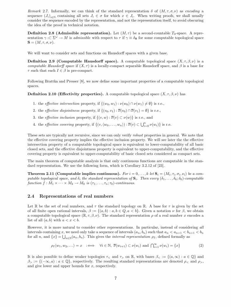
Example 1.2. We now give a simple example which illustrates the difficulties involved in computingreachable sets. Consider the maps fε : R → R given by

fε(x) := ε+ x+ x2 − 9x4, (1)

where ε is a small parameter.

q+(ε)

p−(ε)

p+(ε)

q−(ε)

q+(0)

p(0)

q−(0)

q+(ε)

q−(ε)

(c)(a) (b)

Figure 1: The map f(x) := ε+ x+ x2 − 9x4 for (a) ε < 0, (b) ε = 0 and (c) ε > 0.

For ε = 0, there are fixed points at p(0) = 0, q−(0) = −1/3 and q+(0) = +1/3, as shown in Figure 1(b).Since f ′

0(−1/3) = 5/3 and f ′0(1/3) = 1/3, the fixed points q−(0) and q+(0) are hyperbolic, and can be

continued to give families of fixed points q−(ε) and q+(ε) for some neighbourhood of ε = 0, as shown inFigure 1(a-c). The fixed point p at x = 0 can be continued to two branches of fixed points p−(ε) andp+(ε) for ε < 0, as shown in Figure 1(a), but does not exist for ε > 0, as shown in Figure 1(c).

Since f ′ε(x) = 1 + 2x − 36x3, we can show that f ′

ε(x) > 0 for x 6 5/14, and hence fε is an increasingfunction. If ε > 0 is sufficiently small, then fε(x) > x for all x ∈ (q−(ε), q+(ε)), and fε(x) > x + ε ifx ∈ [−1/3,+1/3].

Consider an initial point x0 ∈ (−1/3, 0). For ε sufficiently close to 0, we have x0 > q−(ε) and x0 < p−(ε)if ε < 0. Let xi = f i

ε(x0) for i ∈ Z+. Then the reachable set of fε starting from x0 is just the orbit{xi : i ∈ Z+}.

If ε < 0, then since q−(ε) < x0 < p−(ε), we have f(q−(ε)) < f(x0) < f(p−(ε)) by monotonicity of fε, soq−(ε) < x1 < p−(ε). Hence xi ∈ (q−(ε), p−(ε)) for all i. Further, since f(x) > x for x ∈ (q−(ε), p−(ε)),the orbit (xi) is an increasing sequence in [x0, p−(ε)]. Indeed, we can show that limi→∞ xi = p−(ε). Inparticular, Reach(fε, {x0} ⊂ [x0, p−(ε)]. Similarly, if ε = 0, we see that Reach(f0, {x0}) ⊂ [x0, 0].

If ε > 0, the situation is very different. Since fε(x) > x + ε for x ∈ (−1/3,+1/3), it must be the casethat xi > 1/3 for some i. In fact, for ε sufficiently small, we have limi→∞ xi = q+(ε). The reachable setis therefore not contained in a small neighbourhood of [x0, 0] for ε > 0, even if ε� 1, and in fact jumpsdiscontinuously at ε = 0.

Hence, to find a good approximation to the reachable set, it is necessary to determine whether ε > 0.If ε is known precisely (e.g. ε is a given rational), then Reach(fε, x0) can be approximated to arbitrary

3

precision. However, if ε is only known approximately, then it may be impossible to decide whether ε > 0,and hence find a good approximation to Reach(fε, x0).

The above example shows that computability of system properties depends on the class of systems underconsideration, and the representation of systems in that class. In the framework of computable analysis, afunction is described approximately; even for a polynomial function with real coefficients, the coefficientsare given by approximating sequences of rationals or rational intervals. In an algebraic framework, suchas polynomial systems with rational coefficients, we can describe a system exactly, and more quantitiesmay be computable. However, the class of systems we can deal with algebraically is restricted comparedwith that of computational analysis.

We could conceive of a reachability algorithm using special techniques for one-dimensional polynomialsystems, and more general techniques for other systems. Unfortunately, the question of whether a one-dimensional continuous function (described in terms of computational analysis) is a polynomial withrational coefficients is undecidable. Hence a dual-method algorithm would need to be told whether itsinput was a polynomial description or an approximate description.

2 Computable analysis and topology

Computable analysis deals with real numbers, continuous functions on real and Euclidean spaces, andsubsets of Euclidean spaces. We consider a more general computable topology dealing with continuousfunctions on Hausdorff spaces. In this section, we review the elements of the literature which we need.The material in Section 2.1 can be found in [20], and that of the other subsections in [23].

2.1 Topological spaces

We first recall the basic facts of general topology.

A topological space is a pair (M, τ) where M is a set and τ is a set of subsets of M (i.e. τ ⊂ P(M)) suchthat

1. ∅ ∈ τ and X ∈ τ ,

2. If U1, U2 ∈ τ , then U1 ∩ U2 ∈ τ , and

3. If U ⊂ τ , then⋃U ∈ τ .

The sets in τ are called open sets, and the complement of an open set is a closed set. A set B is aneighbourhood of a point x if there exists and open set U ∈ τ such that x ∈ U ⊂ B.

A topological space (M, τ) is T0 or Kolmogorov if given any two disjoint points x, x′, there is an openset U containing exactly one of x and x′. The space (M, τ) is T2 or Hausdorff if given any two disjointpoints x, x′, there are disjoint open sets U,U ′ such that x ∈ U and x′ ∈ U ′. The Hausdorff space (M, τ)is T4 or normal if given any two disjoint closed sets A,A′, there are disjoint open sets U,U ′ with A ⊂ Uand A′ ⊂ U ′.

An open cover of a set B ⊂M is a set U ⊂ τ such that B ⊂⋃U . A set C ⊂M is compact if every open

cover of C has a finite subcover. A set B ⊂ M is pre-compact if cl(B) is compact. A topological space(M, τ) is locally compact if every point has a compact neighbourhood.

An open cover U of M is locally finite if for every compact C ⊂M , {U ∈ U : U ∩C 6= ∅} is finite. We sayan open cover U2 is a refinement of a cover U1, denoted U2 ≺ U1, if for all U2 ∈ U2, there exists U1 ∈ U1

such that U2 ⊂ U1. We say a refinement U2 of U1 is a strong refinement, if for all U2 ∈ U2, there existsU1 ∈ U1 such that U2 ⊂ U1, and a proper refinement if for all U1 ∈ U1, U1 =

⋃{U2 ∈ U2 : U2 ⊂ U1}.

A subset β of a topology τ on M is a base for τ if every element of τ is a union of elements of β. If βis a base of τ , then an element U ∈ β is a basic (open) set, and cl(U) is a basic closed set. A subset σ

4

of a topology τ on M is a subbase or generator of τ if τ is the smallest topology containing σ. (i.e. τ isthe smallest subset of P(M) which contains σ and satisfies the axioms for a topology.) A base for thetopology generated by σ is given by all finite intersections of elements of σ.

A topological space is second countable if it has a countable base of open sets. In particular, if a topologyτ has a countable generating set σ, then it has a countable basis (consisting of all finite intersections ofelements of σ).

If (M, τ) is a T0 topological space and σ is a generator for τ , then for any pair x, x′ ∈ M with x 6= x′,there is an element U of σ containing exactly one of x, x′. This means that every point x can be specifiedby giving the subset {U ∈ σ : x ∈ U} of elements of σ containing x.

A sequence (xn) converges to x∞ if for every open set U containing x∞, there exists N ∈ N such thatxn ∈ U for all n > N . If (M, τ) is a Hausdorff space, then any convergent sequence has a unique limit,but otherwise limits need not be unique. (Unique limits for non-Hausdorff spaces can be defined usingconvergent nets.)

Where there is no confusion as to the topology on M , we denote the set of open subsets of a topologicalspace M by O(M), the set of closed subsets by A(M), and the set of compact subsets by K(M).

2.2 Computability and naming systems

We consider computability in terms of words and sequences on a finite alphabet Σ. For digital computers,Σ = {0, 1}, words Σ∗ can be thought of as files or data structures, and sequences Σω can be thoughtof as infinite “data streams”. The binary alphabet {0, 1} can of course be used to represent any otheralphabet, such as the ASCII character set. The alphabet Σ is frequently taken to contain a special blanksymbol , which can denote a space or the end of an input.

Computations are performed by Turing machines with n input tapes and a single output tape. Each inputtape must be specified as either containing a word or a sequence. A partial function f :⊂ Y1, . . . , Yn → Y0

with Yi ∈ {Σ∗,Σω} for i = 0, . . . , n is computable if there is some Turing machine which computesy0 = f(y1, . . . yk), where in the case Y0 = Σ∗ the computation halts with y0 on the output tape, and inthe case Y0 = Σω the computation continuous forever, writing y0 on the output tape.

The theory of computability on words and sequences is known as type-two effectivity (TTE), as opposedto type-one effectivity, which can be considered as “ordinary” computation on words.

In order to formalise computability on more general sets, we consider naming systems.

Definition 2.1 (Naming systems).

1. A notation of a set M is a surjective partial function ν :⊂ Σ∗ →M .

2. A representation of a set M is a surjective partial function δ :⊂ Σω →M .

A notation ν is effective if the set

{(u, v) ∈ Σ∗ × Σ∗ : u, v ∈ dom(ν) and ν(u) = ν(v)}

is recursively enumerable (r.e.).

Note that the domain of an effective notation is recursively enumerable. In most situations of interest,the equivalence problem ν(u) = ν(v) will be recursive (decidable), or even trivial (i.e. ν(u) = ν(v) ⇐⇒u = v.)

Remark 2.2. We could also use functions ν :⊂ N → M as notations, and functions δ : Nω → M asrepresentations.. This is more in the language of recursive function theory, whereas our naming systemsare in the language of Turing computability.

5

Definition 2.3 (Translation and equivalence). Given two naming systems γ :⊂ Y → M and γ ′ :⊂Y ′ → M ′, where Y, Y ′ ∈ {Σ∗,Σω} and M ⊂ M ′, we say a computable function f :⊂ Y → Y ′ translatesγ to γ′ if γ(y) = γ′(f(y)) for all y ∈ dom(γ). We write γ 6 γ ′ if some computable function translates γto γ′. We say γ and γ′ are equivalent, denoted γ ≡ γ ′, if γ 6 γ′ and γ′ 6 γ.

Definition 2.4 (Realisation). Given a function f : M → M ′, and naming systems γ :⊂ Y → M andγ′ :⊂ Y ′ →M ′, a function g : Y → Y ′ is a realisation of f if γ ′(g(y)) = f(γ(y)) for all y ∈ dom(γ).

Given a notation ν of a set M we may wish to give a representation of tuples M ∗ and sequences Mω.There are a number of methods for performing such a “tupling” operation:

1. If Σ contains a blank symbol which is not contained in any word in dom(ν), we can construct arepresentation δ by

δ(w0 w1 w2 · · · ) = (ν(w0), ν(w1), ν(w2), . . .) .

2. If dom(ν) ⊂ Σ∗ is prefix free, then any sequence p ∈ Σω parses uniquely into a sequence p =w0w1w2 · · · with each wi ∈ dom(ν). We can take

δ(w0w1w2 · · · ) = (ν(w0), ν(w1), ν(w2), . . .) .

3. We can construct a wrapping function ı : Σ∗ → Σ∗ such that ı(Σ∗) is prefix-free. One particularchoice for Σ = {0, 1} is

ı(a1a2 · · ·an) = 110a10a20 · · ·0an011.

A representation for Mω is then given by

δ(ı(w0)ı(w1)ı(w2) · · · ) = (ν(w0), ν(w1), ν(w2), . . .).

Regardless of which “tupling” method is chosen, will write 〈w0, w1, w2, . . .〉 for the tupling of words(w0, w1, w2, . . .), and write w � p if p = 〈w0, w1, w2, . . .〉 and w = wi for some i ∈ N. We may also tuplefinitely many words 〈w1, . . . , wk〉, a word and a sequence 〈w, p〉, finitely many sequences 〈p1, . . . , pk〉 oreven infinitely many sequences 〈p1, p2, . . .〉. The tupling of sequences may be effected by shuffling, e.g.〈p1, p2〉 = 〈w1,1, w2,1, w1,2, w2,2, w1,3, w2,3, . . .〉 where pi = 〈wi,1, wi,2, wi,3, . . .〉 for i = 1, 2.

2.3 Computable topological spaces

The essence of a computable topological space is to perform all computations on a countable generatorσ of τ . Computability properties may therefore depend on the generator chosen. To formally relatecomputability concepts to Turing computability, we need a naming system for elements of σ in terms ofsome finite alphabet Σ.

If (M, τ) is a T0-topological space, then every point is specified by the set of open sets containing it. Thisproperty also holds for a generator σ of τ , so every point is specified by {U ∈ σ : x ∈ U}. This gives us away of representing points in topological spaces in a way which respects the topology.

Definition 2.5 (Computable topological space). A computable topological space is a quadruple(M, τ, σ, ν) such that M is a non-empty set, τ ⊂ P(M) is a topology on M , σ ⊂ τ is generator of τ , andν : Σ∗ → σ is an effective notation for σ.

We denote the closures of the elements of σ by ν(w) := cl(ν(w)). We also consider all finite unions of

elements of σ, with notation ν〈w1, . . . wk〉 :=⋃k

i=1 ν(wi).

There is a canonical representation of elements of a computable topological space.

Definition 2.6 (Standard representation). The standard representation δS of a computable topo-logical space S = (M, τ, σ, ν) is the representation δS :⊂ Σω →M given by

δS(p) = x :⇐⇒ {ν(w) : w � p} = {J ∈ σ : x ∈ J}

6

Remark 2.7. Informally, we can think of the standard representation δ of (M, τ, σ, ν) as encoding asequence (Ji)i∈N

containing all sets Ji ∈ σ for which x ∈ Ji. When writing proofs, we shall usuallyconsider the sequence encoded by the representation, and not the representation itself, to avoid obscuringthe idea of the proof in technical notation.

Definition 2.8 (Admissible representation). Let (M, τ) be a second-countable T0-space. A repre-sentation γ :⊂ Σω →M is admissible with respect to τ if γ ≡ δS for some computable topological spaceS = (M, τ, σ, ν).

We will want to consider sets and functions on Hausdorff spaces with a given base.

Definition 2.9 (Computable Hausdorff space). A computable topological space (X, τ, β, ν) is acomputable Hausdorff space if (X, τ) is a locally-compact separable Hausdorff space, and β is a base forτ such that each I ∈ β is pre-compact.

Following Brattka and Presser [8], we now define some important properties of a computable topologicalspaces.

Definition 2.10 (Effectivity properties). A computable topological space (X, τ, β, ν) has

1. the effective intersection property, if {(w0, w1) : ν(w0) ∩ ν(w1) 6= ∅} is r.e.,

2. the effective disjointness property, if {(v0, v1) : ν(v0) ∩ ν(v1) = ∅} is r.e.,

3. the effective inclusion property, if {(v, w) : ν(v) ⊂ ν(w)} is r.e., and

4. the effective covering property, if {(v, 〈w0, . . . , wn〉) : ν(v) ⊂⋃n

i=0 ν(wi)} is r.e.

These sets are typically not recursive, since we can only verify robust properties in general. We note thatthe effective covering property implies the effective inclusion property. We will see later the the effectiveintersection property of a computable topological space is equivalent to lower-computability of all basicclosed sets, and the effective disjointness property is equivalent to upper-computability, and the effectivecovering property is equivalent to upper-computability of basic closed sets considered as compact sets.

The main theorem of computable analysis is that only continuous functions are computable in the stan-dard representation. We use the following form, which is Corollary 3.2.12 of [23].

Theorem 2.11 (Computable implies continuous). For i = 0, . . . , k let Si = (Mi, τi, σi, νi) be a com-putable topological space, and δi the standard representation of Si. Then every (δ1, . . . , δk; δ0)-computablefunction f : M1 × · · · ×Mk →M0 is (τ1, . . . , τn; τ0)-continuous.

2.4 Representations of real numbers

Let R be the set of real numbers, and τ the standard topology on R. A base for τ is given by the setof all finite open rational intervals, β := {(a, b) : a, b ∈ Q, a < b}. Given a notation ν for β, we obtaina computable topological space (R, τ, β, ν). The standard representation ρ of a real number x encodes alist of all (a, b) with a < x < b.

However, it is more natural to consider other representations. In particular, instead of considering allintervals containing x, we need only take a sequence of intervals (an, bn) such that an < an+1 < bn+1 < bnfor all n, and {x} =

⋃n∈N

(an, bn). This gives the interval representation ρI , defined formally as

ρI〈w1, w2, . . .〉 = x :⇐⇒ ∀i ∈ N, ν(wi+1) ⊂ ν(wi) and⋂∞

i=1 ν(wi) = {x} (2)

It is also possible to define weaker topologies τ< and τ> on R, with bases β< := {(a,∞) : a ∈ Q} andβ> := {(−∞, a) : a ∈ Q}, respectively. The resulting standard representations are denoted ρ< and ρ>,and give lower and upper bounds for x, respectively.

7

Euclidean space (Rn, τn) has a base βn consisting of all rational cubes,

βn := {(a1, b1) × · · · × (an, bn) : ai, bi ∈ Q, ai < bi for i = 1, . . . , n} (3)

and becomes a computable Hausdorff space by giving a notation νn for βn. The resulting standard repre-sentation is ρn, which encodes a list of all open cubes containing a point x. An equivalent representationis to use a decreasing sequence of cubes (Ji) such that J i+1 ⊂ Ji and {x} =

⋂∞

i=1 Ji as a name for x.

2.5 Representations of closed sets

We now consider topologies on the set of closed subsets of a second-countable locally compact Hausdorffspace (X, τ). Let β be a base for τ on M , and define

σA< :=

{{A ∈ A(X) : A ∩ J 6= ∅} : J ∈ β

}

σA> :=

{{A ∈ A(X) : A ∩ J 6= ∅} : J ∈ β

}

σA := σA< ∪ σA

> .

(4)

Let τA< , τA> and τA be the topologies generated, respectively, by σA< , σA

> and σA. We denote the topologicalspaces (A(X), τ<), (A(X), τ>) and (A(X), τ) by, respectively, A<(X), A>(X) and A=(X).

We can give representations ψ<, ψ> and ψ for the topologies which are equivalent to the standardrepresentations as follows.

ψ<(p) = A :⇐⇒ {ν(w) : w � p} = {J ∈ β : A ∩ J 6= ∅}

ψ>(p) = A :⇐⇒ {ν(w) : w � p} = {J ∈ β : A ∩ J = ∅}

ψ〈p, q〉 = A :⇐⇒ ψ<(p) = A and ψ>(q) = A.

(5)

The representation ψ< encodes a list of all basic open sets J such that A ∩ J 6= ∅, and ψ> encodes alist of all basic closed sets J such that A ∩ J = ∅. The representations are robust in the sense that ifA∩ J 6= ∅, then there exists I with I ⊂ J such that A∩ I 6= ∅, and if A∩ J = ∅, then there exists I withJ ⊂ I such that A ∩ I = ∅.

A closed subset A of X recursively enumerable if A is ψ<-computable, co-recursively enumerable if it isψ>-computable, and recursive if it is ψ-computable. Note that membership of a recursive set need notbe decidable.

The topologies τA< and τA> are T0 topologies, since given two distinct closed sets A0 and A1, there is apoint x0 of A0 \A1 (or A1 \A0). Then since (X, τ) is normal there is a basic open set J 3 x0 such thatJ ∩ A1 = ∅. Hence A0 ∈ {A ∈ A : A ∩ J 6= ∅} but A1 6∈ {A ∈ A : A ∩ J 6= ∅}. A similar argument showsthat if A0 and A1 are distinct closed sets, then there is a basic closed set J such that J intersects exactlyone of A0 and A1. The topology τA is a normal Hausdorff topology.

The following result on intersection and union operations on closed sets is Theorem 4.1.13 ofWeihrauch [23].

Theorem 2.12.

1. Union (A,B) 7→ A ∪ B on A is (ψ<, ψ<;ψ<)-computable, (ψ>, ψ>;ψ>)-computable and (ψ, ψ;ψ)-computable.

2. Intersection (A,B) 7→ A ∩ B on A is (ψ>, ψ>;ψ>)-computable.

3. The function A 7→ A ∩ {0} is not (τA; τA< )-continuous, and so intersection (A,B) 7→ A ∩ B on Ais not (τA, τA; τA< )-continuous or (ψ, ψ;ψ<)-computable.

We note that, since τA is a stronger topology than τA< , it is immediate that intersection is not(τA, τA; τA)-continuous. Similarly, intersection is not (ψ, ψ, ψ)-computable, or (ψ<, ψ<;ψ<)-computable,since ψ translates to ψ<.

8

2.6 Representations of open sets

Since an open set is the complement of a closed set, we can use the representations of closed sets to giverepresentations of open sets. We let τO< , τO> and τO be the topologies generated, respectively, by σO

< , σO>

and σO defined below:

σO< :=

{{U ∈ O(X) : (X \ U) ∩ J = ∅} : J ∈ β

}=

{{U ∈ O(X) : J ⊂ U} : J ∈ β

}

σO> :=

{{U ∈ O(X) : (X \ U) ∩ J 6= ∅} : J ∈ β

}=

{{U ∈ O(X) : J 6⊂ U} : J ∈ β

}

σO := σO< ∪ σO

> .

(6)

The topologies τO< and τO> are T0 topologies, and τO is a Hausdorff topology. We can give representationsθ<, θ> and θ for the topologies which are equivalent to the standard representations as follows.

θ<(p) = U :⇐⇒ {ν(w) : w � p} = {J ∈ β : J ⊂ U}

θ>(p) = U :⇐⇒ {ν(w) : w � p} = {J ∈ β : J 6⊂ U}

θ〈p, q〉 = U :⇐⇒ θ<(p) = U and θ>(q) = U.

(7)

The representation θ< encodes a list of all basic closed sets J such that J ⊂ U (equivalently(X \ U) ∩ J = ∅) and θ> encodes a list of all basic open sets J such that J 6⊂ U (equivalently(X \ U) ∩ J 6= ∅).

2.7 Representations of compact sets

Let K(X) be the set of compact subsets of X . A subset of a locally compact Hausdorff space is compactif it is closed and bounded. We can specify a bound for a compact C as a finite open cover of C by basicopen sets. The standard representations of compact sets are then given by

κ<〈u, p〉 = C :⇐⇒ C ⊂ ν(u) and ψ<(p) = C

κ>〈u, p〉 = C :⇐⇒ C ⊂ ν(u) and ψ>(p) = C

κ〈u, p, q〉 = C :⇐⇒ C ⊂ ν(u) and ψ〈p, q〉 = C,

(8)

where u ∈ Σ∗ and p, q ∈ Σω. Note that this differs slightly from that of [23], in which only a single basicopen set can be used as a cover. (The representation here is more general, since we do not require thatevery compact set is contained in a single basic open set.)

We can define topologies on compact sets by using generators

σK> :=

{{C ∈ K : C ⊂

⋃k

i=1 Ji} : J1, . . . Jk ∈ β}

σK := σA< ∪ σK

>,(9)

and taking τK> and τK to be the topologies generated, respectively, by σK> and σK. The resulting topo-

logical spaces are K>(X) := (K(X), τK> ) and K=(X) := (K(X), τK).

The standard representations of the computable topological spaces give representations

κcv> (p) = C :⇐⇒ {(ν(w1), . . . , ν(wk)) : 〈w1, . . . , wk〉 � p}

= {(J1, . . . , Jk) ⊂ β : C ⊂⋃k

i=1 Ji}

κcv〈p, q〉 = C :⇐⇒ ψ<(p) = C and κcv> (q) = C.

(10)

The representation κcv> encodes a list of all tuples of basic open sets (J1, . . . , Jk) such that C ⊂

⋃k

i=1 Ji.

The representation is robust, since if C ⊂⋃k

i=1 Ji, then there exists (I1, . . . , Ik) with I i ⊂ Ji for i =

1, . . . , k and C ⊂⋃k

i=1 Ii.

By Lemma 5.2.5 of [23], we have κcv> ≡ κ> and κcv ≡ κ. The equivalence of κ> and κcv

> implies thatevery open cover of C can be computed from a single open cover and a list of basic closed sets disjointfrom C.

9

The situation for lower approximations is rather more complicated. We are not aware of (and conjecturethat there does not exist) a topology on K for which κ< is an admissible representation. However, thetopology τA< |K provides a topology on K for which many operations on compact sets are continuous. Therepresentation κ< strengthens the representation ψ<|K by supplying a bound on the compact set. Hence,for lower approximations, we often consider properties of ψ< as well as κ<, since ψ< is a more naturalrepresentation.

2.8 Representations of continuous functions

The natural topology for the space of continuous functions f : X → Y is the compact-open topology, τ C .This topology is generated by the open sets

σC :={{f ∈ C (X → Y ) : f(C) ⊂ U} : C ∈ K(X), U ∈ O(Y )

}. (11)

The compact-open representation is the standard representation of this topological space, and is given by

δco(p) = f :⇐⇒ {(νX(w1), νY (w2)) : (w1, w2) � p} = {(I, J) ∈ βX × βY : f(I)⊂ J}. (12)

The representation δco encodes a list of pairs (I, J) with I ∈ βX and J ∈ βY for which f(I) ⊂ J .Equivalent to f(I) ⊂ J is I ⊂ f−1(J). The compact-open representation is robust, in the sense that if(I, J) is such that f(I) ⊂ J , then there exist (K,L) with I ⊂ K, L ⊂ J such that f(K) ⊂ L.

As discussed in [23, Chapter 6.1], there are a number of equivalent representation for the space ofcontinuous functions C (X → Y ). In particular, there is a standard representation δ→ under which theevaluation map (f, x) 7→ f(x) and the composition map (g, f) 7→ g ◦ f are computable. The equivalenceof the representation δ→ and the compact-open representation δco is shown by [23, Lemma 6.1.7].

The compact-open representation has the following properties:

Theorem 2.13.

1. The evaluation map (f, x) 7→ f(x) is (δco, ρ; ρ)-computable.

2. The composition map (g, f) 7→ g ◦ f is (δco, δco; δco)-computable.

3. The set-image map (f,A) 7→ cl(f(A)) for A ∈ A(X) is (δco, ψ<;ψ<)-computable.

4. The set-image map (f, C) 7→ f(C) for C ∈ K(X) is (δco, κ<;κ<)-computable, (δco, κ>;κ>)-computable and (δco, κ;κ)-computable.

A representation for sequences is given by the compact-open representation of functions N → X .

The graph of a map f : X → Y is the set

Graph(f) := {(x, y) ∈ X × Y : y = f(x)}.

Since the graph of a continuous function f : X → Y is closed, we can consider the representations ψ<,ψ> and ψ of this set. It turns out that the representation ψ> of A(X × Y ) gives a representation δcc ofC (X → Y ) which is equivalent to the standard representation if Y is compact.

2.9 Union and intersection of sets

We need to extend the results on unions and intersections to the case of infinite unions and intersections.For countable sequences, we use the topology of convergence on finite sequences. Countable unions andintersections have the following computability properties.

Theorem 2.14 (Countable unions and intersections).

10

1. Countable closed union (A1, A2, . . .) 7→ cl(⋃

n∈NAn) on A is (ψ<, ψ<, . . . ;ψ<)-computable.

2. Countable intersection (A1, A2, . . .) 7→⋂

n∈NAn on A is (ψ>, ψ>, . . . ;ψ>)-computable.

3. Countable intersection (C1, C2, . . .) 7→⋂

n∈NCn on K is (κ>, κ>, . . . ;κ>)-computable.

Proposition 2.15.

1. Countable closed union is neither (τA, τA, . . . ; τA> )-continuous nor (τK, τK, . . . ; τK> )-continuous.

2. Countable intersection is neither (τA, τA, . . . ; τA< )-continuous nor (τK, τK, . . . ; τK< )-continuous.

The proofs are straightforward.

3 Multivalued maps

In system theory, it is useful to consider multivalued maps F : X ⇒ Y , since these represent controlsystems f : X × U → X as F (x) = f(x, U).

We typically represent a multivalued map F : X ⇒ Y by a single-valued map X → P(Y ), but mayalso identify F with its graph, Graph(F ) := {(x, y) ∈ X × Y : y ∈ F (x)}. If A ∈ P(X), then we defineF (A) := {y ∈ Y : ∃x ∈ A, y ∈ F (x)}. Thus a multivalued map F : X ⇒ Y induces a single valued mapP(X) → P(Y ). If F : X ⇒ Y and G : Y ⇒ Z, the composition of F and G is G ◦ F : X ⇒ Z given byG ◦ F (x) := G(F (x)) = {z ∈ Z : ∃ y ∈ Y, y ∈ F (x) and z ∈ G(y)}. Note that G ◦ F (A) = G(F (A)), andcomposition is associative.

There are two natural set-valued preimages of F : X ⇒ Y , the weak preimage F−1(B) = {x ∈ X :F (x) ∩ B 6= ∅}, and the strong preimage, F⇐(B) = {x ∈ X : F (x) ⊂ B}. The graph of F−1 is the“transpose” of the graph of F ; i.e. (x, y) ∈ Graph(F ) ⇐⇒ (y, x) ∈ Graph(F−1). If F : X ⇒ X , thenan orbit of F is a sequence (xi) such that xi+1 ∈ F (xi) for all i, so the reverse of an orbit of F is an orbitof F−1.

We say F is lower-semicontinuous if F−1(U) is open whenever U is open, or equivalently, if F⇐(A)is closed whenever A is closed. F is upper-semicontinuous if F−1(A) is closed whenever A is closed,or equivalently, if F⇐(U) is open whenever U is open. A function F is weakly upper-semicontinuousif F−1(C) is closed whenever C is compact. A multivalued function is continuous if it is both lower-semicontinuous and upper-semicontinuous.

Henceforth, we restrict attention to functions with closed values, which means that F (x) is closed forall x, denoted F : X → A(Y ). We also consider functions with compact values, which means F (x) iscompact for all x, denoted or F : X → K(Y ).

A closed-valued function F : X → A(Y ) is lower-semicontinuous if, and only if, it is (τX ; τA(Y )< )-

continuous, and weakly upper-semicontinuous if, and only if, it is (τX ; τA(Y )> )-continuous. A compact-

valued function F : X → K(Y ) is upper-semicontinuous if, and only if, it is (τX ; τK(Y )> )-continuous.

If F is locally-bounded, then F is (strongly) upper-semicontinuous if F : X → K>(Y ) is continuous. Amultivalued function is continuous if it is both lower-semicontinuous and upper-semicontinuous.

We denote closed-valued lower-semicontinous functions by LSCA, closed-valued weakly upper-semicontinuous functions by USCA, and compact-valued upper semicontinous functions by USCK. Wedenote closed-valued weakly continuous functions by CA and compact-valued continuous functions byCK.

If F ∈ LSCA, then F (cl(A)) ⊂ cl(F (A)) for any set A, and therefore cl(G ◦ F (x)) = cl(G(cl(F (x)))).If F ∈ USCA, then F (C) is closed whenever C is compact, and F ∈ USCK, then F (C) is compactwhenever C is compact, but in both cases F (A) need not be closed even if A is closed. If F ∈ USC A if,and only if, Graph(F ) is closed.

11

Upper-semicontinuity with compact values is preferable to weak upper-semicontinuity with closed values,since (strong) upper-semicontinuity is preserved under composition.

For a closed-valued lower-semicontinuous function F , the image F (A) need not be closed even if A isclosed. This means that the composition (F,G) 7→ F ◦G need not be closed-valued. We therefore take aclosed-valued composition (F,G) 7→ cl(F ◦G) defined by cl(F ◦G) (x) := cl(F (G(x))).

For more information on multivalued functions, see Klein and Thompson [14].

3.1 Topology of multivalued semicontinuous functions

To define topologies on the spaces of closed-valued (semi)continuous maps, we identify LSC A(X ⇒ Y )with C (X → A<(Y )), USCA(X ⇒ Y ) with C (X → A>(Y )) and CA(X ⇒ Y ) with C (X → A(Y )),and use the compact-open topologies. Explicit generators for the topologies τMA

< on LSCA and τMA> on

LSCK are given by

σMA< :=

{{F ∈ LSCA : I ⊂ F−1(J)} : I ∈ βX , J ∈ βY

},

σMA> :=

{{F ∈ USCA : I ∩ F−1(J) = ∅} : I ∈ βX , J ∈ βY

}.

(13)

Note that I ⊂ F−1(J) ⇐⇒ ∀x ∈ I, F (x) ∩ J 6= ∅, and that I ∩ F−1(J) = ∅ ⇐⇒ F (I) ∩ J = ∅.

The lower-semicontinuous functions LSCK(X ⇒ Y ) are somewhat degenerate, and have no naturaltopology other than that induced from LSCA(X ⇒ Y ). To define topologies on the spaces of compact-valued (semi)continuous maps, we identify USCK(X ⇒ Y ) with C (X → K>(Y )) and CK(X ⇒ Y ) withC (X → K(Y )), and again use the compact-open topologies. An explicit generator for the topology τMK

>

on USCK is

σMK> :=

{{F ∈ USCK : I ⊂ F⇐(

⋃k

i=1 Ji)} : I ∈ βX , J1, . . . Jk ∈ βY

}. (14)

Note that I ⊂ F⇐(⋃k

i=1 Ji) ⇐⇒ F (I) ⊂⋃k

i=1 Ji.

3.2 Representations of multivalued semicontinuous functions

We now define representations µ< for lower-semicontinuous maps, µA> for weakly upper-semicontinuous

maps, and µK> for upper-semicontinuous compact-valued maps.

Admissible representations for τMA< , τMA

> and τMA are given by

µA<(p) = F ∈ LSCA :⇐⇒ {(νX(v), νY (w)) : 〈v, w〉 � p}

= {(I, J) ∈ βX × βY : I ⊂ F−1(J)},

µA>(p) = F ∈ USCA :⇐⇒ {(νX(v), νY (w)) : 〈v, w〉 � p}

= {(I, J) ∈ βX × βY : I ∩ F−1(J) = ∅}

µA〈p, q〉 = F ∈ CA :⇐⇒ µA<(p) = µA

>(q) = F.

(15)

Note that µA< encodes a list of all pairs (I, J) with I ∈ βX , J ∈ βY such that I ⊂ F−1(J) (equivalently,

∀x ∈ I, F (x)∩J 6= ∅), and µA> encodes a list of all pairs (I, J) with I ∈ βX , J ∈ βY such that F (I)∩J = ∅.

An admissible representation for compact-valued upper-semicontinous functions is given by

µK>(p) = F ∈ USCK :⇐⇒ {(νX(v), νY (w1), . . . , νY (wk)) : 〈v, w1, . . . , wk〉 � p}

= {(I, J1, . . . , Jk) : I ⊂ F−1(⋃k

i=1 Ji)}.(16)

Note that µK> encodes a list of all tuples (I, J1, . . . , Jk) such that F (I) ⊂

⋃k

i=1 Ji.

The following result on representations is immediate from the definitions.

Lemma 3.1.

12

1. The representations µA< of LSCA(X ⇒ Y ) and δco of C (X → A<(Y )) are equivalent.

2. The representations µA> of USCA(X ⇒ Y ), δco of C (X → A>(Y )), and ψ> of Graph(F ) are

equivalent.

3. The representations µK> of USCA(X ⇒ Y ) and δco of C (X → K>(Y )) are equivalent.

For single-valued maps, the situation is simpler.

Lemma 3.2. The representations δco, µA<, µK

>, and µK are equivalent representations for C (X → Y ).

Proof. The representations δco and µA< are trivially equivalent, since f(C) ⊂ U if, and only if, ∀x ∈ C,

f(x)∩U 6= ∅. We need then only show that µA< and µK

> are equivalent, since the other equivalences followby definition.

µA< 6 µK

>:

We need to compute a list of all (K,L1, . . . , Ll) with f(K) ⊂⋃l

j=1 Lj from a list of all (I, J) with f(I) ⊂ J .

We claim that an algorithm which outputs (K,L1, . . . , Ll) if there exists a finite set {(Ii, Ji) : i = 1 . . . k}

with F (I i) ⊂ Ji for i = 1, . . . k such that K ⊂⋃k

i=1 Ii and J i ⊂⋃l

j=1 Lj (covering) for all i = 1, . . . , kperforms the calculation.

If (K,L1, . . . , Ll) is output, then F (I i) ⊂ Ji, K ⊂⋃k

i=1 Ii and J i ⊂⋃l

j=1 Lj , so F (K) ⊂⋃l

j=1 Lj .

If F (K) ⊂⋃l

j=1 Lj , then every x ∈ K has a neighbourhood Ix such that F (Ix) ⊂ Jx with Jx ⊂⋃l

j=1 Lj .

Since K is compact, there is a finite subset {xi : i = 1, . . . , k} with K ⊂⋃k

i=1 Ixi. Hence (K,L1, . . . , Ll)

is output.

µK> 6 µA

<:We need to compute a list of all (I, J) with f(I) ⊂ J from a list of all (K,L1, . . . , Ll) such that f(K) ⊂⋃l

j=1 Lj . To do this, we simply output (I, J) = (K,L1) if F (K) ⊂⋃l

j=1 Lj with l = 1.

3.3 Counterexamples for multivalued functions

We now give some examples illustrating counterexamples for multivalued semicontinuous functions.

The following example shows that a map F : X → A>(Y ) may have F (x) compact for all x ∈ X , butnot be continuous as a map F : X → K>(Y ).

Example 3.3. Let F : R ⇒ R be given by F (x) = {0} if x 6 0, and F (x) = {0, 1/x} if x > 0. ThenF : R → A>(R) is continuous, but F−1(−1, 1) = (−∞, 0]∪(1,∞) which is not open, and F⇐[1,∞) = (0, 1]which is not closed, so is not upper-semicontinuous with compact values.

If G(x) = {0} if x < 1, and G(x) = {0, 1} for x > 1, then G is upper semicontinuous, but G ◦F (x) = {0}if x ∈ (−∞, 0] ∪ (1,∞) and G ◦ F (x) = {0, 1} if x ∈ (0, 1], so G ◦ F is not upper semicontinuous.

Rather than consider compact-valued maps, we could consider, with more generality, closed-valuedmaps. However, the composition of two closed-valued upper-semicontinuous maps need not be upper-semicontinuous, as Example 3.4 shows.

Example 3.4. Let F (x) = {0, 1/x} for x > 0, and F (0) = {0} . Let G(x) = {0, 1} if x > 1 andG(x) = {0} if x < 1. Then G ◦ F (x) = {0} if x = 0 or x > 1, and G ◦ F (x) = {0, 1} if 0 < x 6 1. HenceG ◦ F is not upper-semicontinuous.

We could also consider the representation ψ< of Graph(F ) on A(X × Y ) as a lower representation forUSC (X ⇒ Y ). It is straightforward to show that µ< 6 ψ< on USC (X ⇒ Y ). However, a ψ< is strictlyweaker than µ<, even for continuous functions, as the following example shows.

13

(a) Fn

(b) F

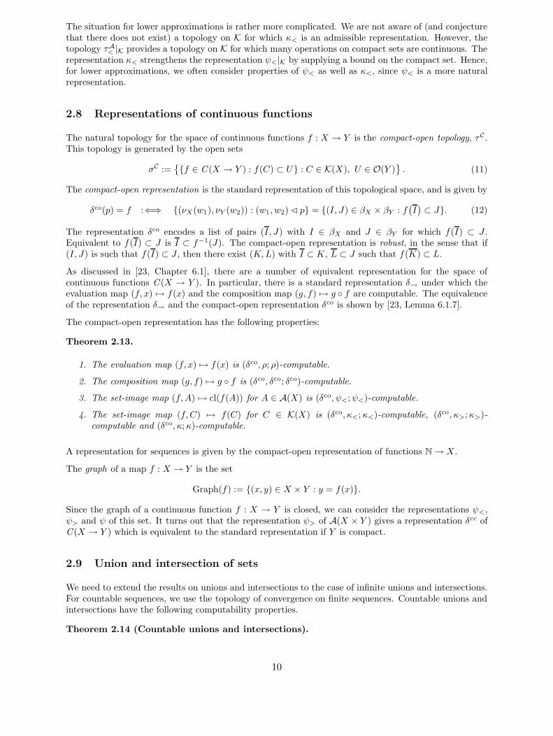
Figure 2: The limit of a continuous multivalued map may exist in the graph topology but notthe compact-open topology. (a) Fn, (b) the limit F .

Example 3.5. Let g(x) : [−1, 1] → [−1, 1] be continuous, and let Fn(x) = {g(x) sin(nx)}. Then in theτA topology on A(X × Y ), Graph(Fn) → {(x, y) : |y| 6 |g(x)|} = Graph(F ), a continuous multivaluedmap, but Fn does not converge in the compact-open topology τM< on multivalued maps, since if C iscompact and U = (0, 1), then (C,U) is a pair such that ∀x ∈ C, F (x) ∩ U 6= ∅ and U ⊂ (0, 1), then forsufficiently large n, ∃xn ∈ C with sin(nxn) < 0, and then Fn(xn) ∩ U = ∅. Hence Fn does not convergeto F .

3.4 Composition of multivalued maps

We now show that composition of multivalued maps, where continuous, is computable in the appropriaterepresentation.

Theorem 3.6.

1. The closed composition function (F,G) 7→ cl(F ◦G) is (µA<, µ

A<;µA

<)-computable.

2. The composition function (F,G) 7→ F ◦G is (µA>, µ

K>;µA

>)-computable and (µA, µK;µA)-computable.

3. The composition function (F,G) 7→ F ◦G is (µK>, µ

K>;µK

>)-computable and (µK, µK;µK)-computable.

Proof. (F,G) 7→ cl(F ◦G) is (µA<, µ

A<;µA

<)-computable:

Output (I,K) if there exists a finite set {(Ii, Ji) : i = 1 . . . k} such that I ⊂⋃k

i=1 Ii (covering), I i ⊂G−1(Ji), and J i ⊂ F−1(K).

If (I,K) is output, then ∀x ∈ I , ∃i with x ∈ Ii. Then G(x)∩Ji 6= ∅, so ∃y ∈ G(x)∩Ji, and F (y)∩K 6= ∅since y ∈ J i, so F ◦G(x) ∩K 6= ∅.

Conversely, if I ⊂ (F ◦ G)−1(K), then ∀x ∈ I , ∃y ∈ Y, z ∈ K with y ∈ G(x) and z ∈ F (y). Henceby lower-semicontinuity, ∃Jx such that y ∈ Jx and z ∈ F (Jx), so Jx ⊂ F−1(K). Similarly, ∃Ix suchthat x ∈ Ix and Ix ⊂ G−1(Jx). Since I is compact, there is a finite subset {xi : i = 1, . . . , k} with

I ⊂⋃k

i=1 Ixi. Hence (I,K) is an output.

(F,G) 7→ F ◦G is (µA>, µ

K>;µA

>)-computable:

Output (I,K) if there exists a finite set {J1, . . . , Jk} such that G(I) ⊂⋃k

i=1 Ji and F (J i) ∩K = ∅ fori = 1, . . . , k.

If (I,K) is output, then G(F (I)) ⊂ G(⋃k

i=1(Ji)) ⊂⋃k

i=1G(J i), so G ◦ F (I) ∩K = ∅.

Conversely, suppose F (G(I)) ∩K = ∅. Since F is weakly upper-semicontinuous, F−1(K) is closed, andso V = F⇐(Z \K) is open. Hence G(I) ⊂ V , and since G is compact-valued upper-semicontinuous, G(I)

is compact. Thus there exist J1, . . . , Jk such that G(I) ⊂⋃k

i=1 Ji and J i ⊂ V for i = 1, . . . , k. HenceF (J i) ∩K = ∅ for i = 1, . . . , k, and so (I,K) is output.

14

(F,G) 7→ F ◦G is (µA, µK;µA)-computable:Immediate since (F,G) 7→ F ◦G is (µA

<, µA<, µ

A<)-computable and (µA

>, µK>, µ

A>)-computable.

(F,G) 7→ F ◦G is (µK>, µ

K>;µK

>)-computable:

Output (I,K1, . . .Kk) if ∃ J1, . . . Jm such that G(I) ⊂⋃m

j=1 Jj and F (J j) ⊂⋃k

i=1 Ki for j = 1, . . . ,m.

If (I,K1, . . . ,Kk) is output, then F ◦G(I) ⊂ F (⋃m

j=1 Jj) and F (J j) ⊂⋃k

i=1 Ki for all j, so F ◦G(I) ⊂⋃k

i=1Ki.

Conversely, if F ◦G(I) ⊂⋃k

i=1 Ki, then F (y) ⊂⋃k

i=1 Ki for all y ∈ G(I). By upper-semicontinuity, for

each y ∈ G(I), there exists Jy such that F (Jy) ⊂⋃k

i=1Ki, and since G(I) is compact, there is a finite

subset {y1, . . . ym} of G(I) such that G(I) ⊂⋃m

j=1 Jyj. Then G(I) ⊂

⋃m

j=1 Jyjand F (Jyj

) ⊂⋃k

i=1Ki for

j = 1, . . .m. Hence (I,K1, . . . ,Kk) is output.

(F,G) 7→ F ◦G is (µK, µK;µK)-computable:Immediate since (F,G) 7→ F ◦G is (µA

<, µA<, µ

A<)-computable and (µK

>, µK>, µ

K>)-computable.

A closed set A can be considered as a function from a one-point space 1 to A. Then the representationsψ<, ψ> and ψ of A(X) are equivalent, respectively, to µA

<, µA> and µA of C (1 ⇒ X). Similarly, the

representations κ<, κ> and κ of K(X) are equivalent, respectively, to µK<, µK

> and µK of CK(1 ⇒ X).This gives the following

Corollary 3.7.

1. The function (F,A) 7→ cl(F (A)) is (µA<, ψ<;ψ<)-computable.

2. The function (F,C) 7→ F (C) is (µA>, κ>;ψ>)-computable and (µA, κ;ψ)-computable.

3. The function (F,C) 7→ F (C) is (µK>, κ>;κ>)-computable and (µK, κ;κ)-computable.

If F is an upper-semicontinuous map, then F (A) need not be closed even if A is closed. We can considerthe composition function (F,A) 7→ cl(F (A)) for F ∈ USCK and A ∈ A, and attempt to compute aψ>-name of cl(F (A)). However, the following result shows that this is impossible.

Theorem 3.8. The function (F,A) 7→ cl(F (A)) is not (τMK, τA; τA> )-continuous.

Proof. Let A = [0,∞), and Fa(x) = {0} if x 6∈ [a − 1, a+ 1], Fa(x) = [0, x − a + 1] if x ∈ [a− 1, a] andFa(x) = [0, a+ 1 − x] if x ∈ [a, a+ 1]. Then Fa → F given by F (x) = {0} as a → ∞, but Fa(A) = [0, 1]which does not converge to F (A) = {0}. Hence (F,A) 7→ cl(F (A)) is not (τMK, τA; τA> )-continuous.

4 Reachability problems

We now apply the material developed in Section 3 to the study of the reachability problem for semicon-tinuous systems. We first define the reachable, closed-reachable and chain-reachable sets, and give analternative formulation of the chain reachable set. We then prove some straightforward results on com-putability of countable unions and intersections, and use these to prove the main results on reachability.Finally, we discuss closure-interior systems, which have inner as well as outer approximations, and showthat the computability results extend to these systems as well.

4.1 Reachable and chain reachable sets

Definition 4.1 (Reachability). Let F : X ⇒ X be a multivalued map, and X0 ⊂ X . Then thereachable set of F from X0 is

Reach(F,X0) := {y ∈ X : ∃x0, x1, . . . xn such thatx0 ∈ X0, (xi, xi+1) ∈ F for i = 0, . . . , n− 1, and xn = y.

(17)

15

The reachable set need not be closed, so we take its closure, and define the closed reachable set as

Reach(F,X0) := cl(Reach(F,X0)). (18)

We now briefly recall the concepts of ε-chains as considered by Conley [10]. If (X, d) is a metric spaceand F : X ⇒ X is a multivalued map, then a sequence of points x0, x1, . . . , xn is an ε-chain if there existy1, . . . , yn ∈ X with yi+1 ∈ F (xi) and d(yi+1, xi+1) < ε for i = 0, . . . , n− 1. A point x is ε-reachable froma set X0 if there is an ε-chain x0, x1, . . . , xn with x0 ∈ X0 and xn = x. A point x is chain-reachable fromX0 if there is an ε-chain from X0 to x for all ε > 0.

The concept of chains can be generalised to non-metric spaces as follows:

Definition 4.2 (U-chain). Let U be an open cover, and F : X ⇒ X . A sequence x0, . . . , xn is aU-chain for F if there exist points y1, . . . , yn ∈ X and open sets U1, . . . , Un ∈ U such that yi+1 ∈ F (xi)and xi+1, yi+1 ∈ Ui+1 for i = 0, . . . , n− 1.

Equivalently, we can define the U-neighbourhood of a set B by NU(B) :=⋃{U ∈ U : B ∩ U 6= ∅}. Then

a sequence x0, . . . , xn is a U-chain for F if, and only if, xi+1 ∈ NU (F (xi)) for i = 0, . . . , n− 1.

Definition 4.3 (Chain reachability). Let F : X ⇒ X be a multivalued map, and X0 ⊂ X . Define

Reach(F,X0,U) := {x ∈ X : ∃ U-chain x0, x1, . . . , xn for F such that x0 ∈ X0 and xn = x} (19)

the set of points reachable from X0 by a U-chain. The chain reachable set of F from X0 is

ChainReach(F,X0) :=⋂

U Reach(F,X0,U), (20)

where U runs over all locally finite open covers of X .

It is straightforward to show [10] that ChainReach(F,X0) is closed for any system F and any initial setX0. An equivalent definition of the chain reachable set of an upper-semicontinuous closed-valued functioncan be given in terms of graphs.

ChainReach(F,X0) =⋂

{Reach(G,X0) : G ∈ LSCO and Graph(F ) ⊂ Graph(G)} (21)

We now give an alternative characterisation of the chain reachable set which will be useful when per-forming a computability analysis. We use the following lemma on compact chain-reachable sets.

Lemma 4.4. If ChainReach(F,C) is compact, then for any open neighbourhood U of ChainReach(F,C),there exists an open cover U such that cl(Reach(F,C,U)) ⊂ U . In particular, there exists an open coverU such that Reach(F,C,U) is pre-compact.

Proof. Suppose ChainReach(F,C) is compact, and let V be a pre-compact open neighbour-hood of ChainReach(F,C) such that cl(V ) ⊂ U . Then since F is upper-semicontinuous andF (ChainReach(F,C)) ⊂ ChainReach(F,C), we see that F⇐(V ) is an open neighbourhood ofChainReach(F,C). Hence there is an open neighbourhood W of ChainReach(F,C) such that cl(W ) ⊂ Vand F (cl(W )) ⊂ V . Choose an open cover V such that NV(F (cl(W ))) ⊂ V , and let B = cl(V ) \W , acompact set. Now if U is any refinement of V , then either Reach(F,C,U) ⊂W , or there exists a U-chainx0, x1, . . . , xn with x0 ∈ C, xi ∈ W for i < n and xn 6∈ W . Then xn ∈ NU (F (xn−1)) ⊂ NV(F (cl(W ))) ⊂V , so xn ∈ B, and hence cl(Reach(F,C,U)) ∩ B 6= ∅. Since cl(Reach(F,C,U)) decreases on taking re-finements, and converges to ChainReach(F,C,U), we must have cl(Reach(F,C,U)) ∩ B = ∅ for some U .Then cl(Reach(F,C,U)) ⊂W , so cl(Reach(F,C,U)) ⊂ U and Reach(F,C,U) is pre-compact.

Theorem 4.5 (Characterisation of the chain-reachable set). Let F ∈ USCK and C a compactset. Suppose ChainReach(F,C) is compact. Then

ChainReach(F,C) =⋂{U ∈ O(X) : C ⊂ U and F (cl(U)) ⊂ U}. (22)

16

Proof. We first show that for any neighbourhood V of ChainReach(F,C), there exists U ⊂ V with C ⊂ Uand F (cl(U)) ⊂ U . For any open cover U , we have C ⊂ Reach(F,C,U) and cl(F (Reach(F,C,U))) ⊂Reach(F,C,U). By Lemma 4.4, if V is any open neighbourhood of ChainReach(F,C), then thereis an open cover U such that cl(Reach(F,C,U)) ⊂ V . Hence there is an open set U such thatC ∪ cl(F (Reach(F,C,U))) ⊂ U and cl(U) ⊂ Reach(F,C,U). Then U ⊂ V , C ⊂ U and F (cl(U)) ⊂F (Reach(F,C,U)) ⊂ cl(F (Reach(F,C,U))) ⊂ U as required.

To complete the proof, we let U be such that C ⊂ U and F (cl(U)) ⊂ U , and need to show thatChainReach(F,C) ⊂ U . We have NU(F (cl(U))) ⊂ U for some open cover U . Defining sets Xn recursivelyby Xn+1 := NU(F (Xn)), we see by induction that Xn ⊂ U for all n, so Reach(F,C,U) ⊂ U and henceChainReach(F,C) ⊂ U .

To consider computability of the reachable and chain reachable sets, we reformulate the reachabilityconditions as operators. The closed reachability operator naturally operates on lower-semicontinuousmaps, and the chain reachability operator on upper-semicontinuous maps.

Definition 4.6 (Reachability operators).

1. The closed reachability operator is the function Reach : LSC A(X ⇒ X)×A(X) → A(X) given byReach(F,A) := cl(Reach(F,A)).

2. The chain reachability operator is the function ChainReach : USCK(X ⇒ X) × A(X) → A(X)given by ChainReach(F,A) :=

⋂U

Reach(F,A,U), where U runs over all locally-finite open covers.

The following example shows that the chain reachability operator may be badly behaved if the chain-reachable set is not compact.

−1

−1

Fa(x)

0 a+1aa−1 x

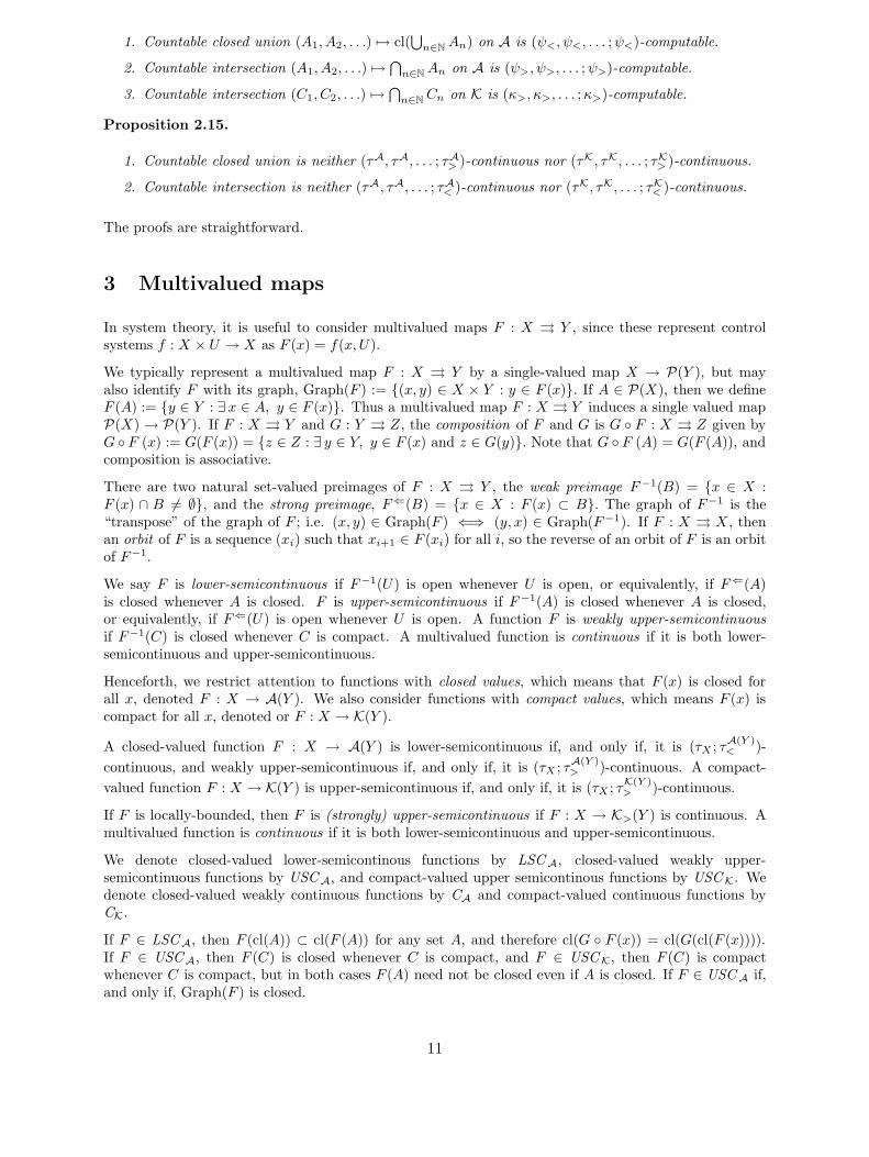
Figure 3: The map Fa of Example 4.7.

Example 4.7. Define continuous multivalued maps F : R ⇒ R and Fa : R ⇒ R by

F (x) :=

{{0} if x 6 0,

{0, x} if x > 0Fa(x) :=

F (x) ∪ {a− 1 − x} if x ∈ [a− 1, a],F (x) ∪ {x− a− 1} if x ∈ [a, a+ 1],

F (x) otherwise.(23)

The graph of Fa is shown in Figure 3. Note that Fa → F as a → ∞ in τMK, since for any compact setC, Fa|C = F |C for a sufficiently large, and that F (x) ⊂ Fa(x) for all x.

Let X0 = {0}, and consider chain reachable sets ChainReach(F,X0). We have ChainReach(F, {0}) =[0,∞), since we can reach any point in [0,∞) from 0 by an ε-chain (xi) by taking yi+1 = xi as x ∈ F (x)for all x, and xi+1 > yi. Since Fa(x) ⊃ F (x) for any x, we must have ChainReach(Fa, {0}) ⊃ChainReach(F, {0}) for any a. Hence [a − 1, a + 1] ⊂ ChainReach(Fa, {0}), and so [−1, 0] ⊂ChainReach(Fa, X0), since Fa([a − 1, a + 1]) ⊂ [−1, 0]. Thus ChainReach(Fa, {0}) = [−1,∞) for anya.

We therefore have a situation in which Fa → F in µK as a → ∞, but ChainReach(Fa, {0}) does notconverge to ChainReach(F, {0}) as a→ ∞ in τA> .

17

4.2 Computability of reachable sets

We now consider the computability of the closed reachability operator and the chain reachability operator.We find that the closed reachability operator is lower-computable in all cases, and the chain reachabilityoperator is upper-computable if the chain-reachable set is compact. Using these results, we can obtainsemi-decision algorithms for verification of system properties.

Theorem 4.8 (Computability of closed reachability).

1. The closed reachability operator for lower-semicontinuous discrete-time systems is (µA<, ψ<;ψ<)-

computable.

2. The closed reachability operator for bounded discrete-time systems is not (τMK, τK; τK> )-continuous.

Proof. 1. Since (F,A) 7→ cl(F (A)) is (µA<, ψ<, ψ<)-computable, and the function (F,A) 7→ Ai :=

cl(F i(A)) is (µA<, ψ<, ψ<)-computable for all i ∈ N. Since Reach(F,A) := cl(

⋃∞

i=0 Fi(A)) =

cl(⋃∞

i=0 Ai), and countable closed union is (ψ<, ψ<, . . . ;ψ<)-computable, the result follows.

2. Consider the system fε defined in Section 1.2. Then fε → f0 in τMK, and {q−(ε)} → {q−(0)} inτK, but Reach(fε, [q−(ε), 0]}) = [q−(ε), q+(ε)] for ε > 0, which does not converge to [q−(0), 0] =Reach(F0, [q−(0), 0]) in τK> .

We can Theorem 4.8(1) to verify system controllability. Suppose we wish to check whether it is possibleto reach an open set U starting from some initial point x. We compute a ψ<-name of Reach(F, {x}), andverify controllability if the ψ<-name contains some set J with J ⊂ U . If the set is not reachable, thenthe procedure does not terminate.

Theorem 4.9 (Computability of chain reachability).

1. If ChainReach(F,C) is compact, then (F,C) 7→ ChainReach(F,C) is (µK>, κ>;κ>)-computable.

2. The map (F,C) 7→ ChainReach(F,C) is not (τMK, τK, τA> )-continuous.

3. The map (F,C) 7→ ChainReach(F,C) is not (τMK, τK; τA< )-continuous.

Proof. 1. A κ> name of C encodes a list of all basic open covers of C. A µK>-name of F encodes

a list of all tuples (I, J1, . . . , Jk) such that F (I) ⊂⋃k

i=1 Ji For each basic open cover {I1, . . . , Ik}

of C, we let U =⋃k

j=1 Ij . Then F (cl(U)) ⊂ U if, and only if, F (I i) ⊂⋃k

j=1 Ij for all i. Hence

we can compute a list of all open U with A ⊂ U such that U =⋃k

j=1 Ij and F (cl(U)) ⊂ U . ByTheorem 4.5, the intersection of all such U equals ChainReach(F,A), hence we have computed aκ>-name of ChainReach(F,A).

2. Consider the systems Fa of Example 4.7. Then Fa → F∞ in τMK as a → ∞. However,ChainReach(Fa, {0}) = [1,∞) whereas ChainReach(F∞, {0}) = [0,∞), so ChainReach(Fa, {0})does not converge to ChainReach(F∞, {0}) in τA> . Hence (F,C) 7→ ChainReach(F,C) is not(τMK, τK, τA> )-continuous. (A similar example can be made in two-dimensions with a single-valuedcontinuous map.)

3. Consider the map fε defined in Example 1.2. Then {p−(ε)} → {0} in τκ as ε → 0. We haveChainReach(fε, {p−(ε)}) = {p−(ε)} for ε < 0, and ChainReach(f0, {0}) = [0, q+(ε)]. HenceChainReach(fε, {p−(ε)}) does not converge to ChainReach(f0, 0) in τA< . Therefore (F,C) 7→ChainReach(F,C) is not (τMK, τK; τA< )-continuous.

We can use the chain reachable set to check safety properties of a system, that is, whether it is possible toleave an open set S of safe states starting from some initial set X0. We compute a κ>-representation ofChainReach(F,X0), and verify safety if there exists some open cover {J1, . . . , Jk} of ChainReach(F,X0)

such that the set U :=⋃k

i=1 Ji with ChainReach(F,X0) ⊂ U is a subset of S.

18

We say that reachable set is robust if Reach(F,A) = ChainReach(F,A). We have seen that we cancompute inner and outer approximations to Reach(F,A) if the reachable set is robust. The followingresult shows that this condition is sharp.

Theorem 4.10 (Uncomputability of reachability). The closed reachable set is (µK, κ;κ)-computableif and only if it is robust.

Proof. We have already shown that Reach(F,A) is computable if Reach(F,A) = ChainReach(F,A).

Conversely, suppose Reach(F,A) 6= ChainReach(F,A). Let Fn be a sequence of continuous multivaluedmaps converging to F such that Graph(F ) ⊂ int(Graph(Fn)) for all n. Then ChainReach(F,A) ⊂Reach(Fn, A) for all n, and Reach(Fn, A) → ChainReach(F,A) as n→ ∞.

For any name p of F , there is a sequence pn of names of Fn such that pn → p, since any elements ina µA

<-name of F are present in a µA<-name of Fn, and for n sufficiently large, the first m elements of

p give rise to sets disjoint from Graph(F ). Any computation of the first m elements of ψ>-name ofReach(F,A) depends only on the first k elements of a ψ-name of F , and hence is equal to the first melements of a ψ>-name of Reach(Fn, A) for n sufficiently large. In particular, the first m elements of aψ>-name of Reach(F,A) are disjoint from Reach(Fn, A), and hence from ChainReach(F,A). Since thisis true for any m ∈ N, we see that it is impossible to compute a lower bound for Reach(Fn, A) smallerthan ChainReach(F,A).

4.3 Closure-interior systems

A set which is the closure of its interior may be both inner- and outer-approximated.

Definition 4.11 (Closure-interior sets). A set A is a closure-interior or clint set if A = cl(int(A)).We denote the set of all closure-interior subsets of X by CI(X).

If A ∈ CI(X), then the set U := int(A) satisfies U = int(cl(U)). Conversely, if U = int(cl(U)), thenA := cl(U) ∈ CI(X).

Unlike general closed sets which admit outer approximations but not inner approximations (we use lowerapproximations instead), clint sets admit natural outer and inner approximations. We use a representationcombining a θ<-name for int(A) (as defined in Section 2.6) and either a ψ>-name or a κ>-name for A,as appropriate.

A continuous function F such that Graph(F ) is a clint set may be specified by a ψ>-name or κ>-namefor Graph(F ), and by a θ<-name for Graph(G) where G is defined by Graph(G) = int(Graph(F )). Notethat a function G is lower-semicontinuous with open values if, and only if, Graph(G) is open, and ifG1 and G2 have open graphs, then so does G1 ◦ G2.The following theorem shows that continuous clintsystems behave nicely when operating on sets.

Theorem 4.12. If G is a continuous, open-valued function, and U is open, then cl(G(U)) = F (cl(U)),where Graph(F ) = cl(Graph(G)).

Proof. Clearly cl(G(U)) ⊂ F (cl(U)) since F (cl(U)) is closed. Suppose y 6∈ cl(G(U)). Then there existsa neighbourhood Z of y such that Z ∩ G(U) = ∅. Then G−1(Z) ∩ U = ∅, and since Z is open and Gis lower-semicontinuous, G−1(Z) ∩ cl(U) = ∅. Choose a neighbourhood W of y with cl(W ) ⊂ Z. ThenG−1(cl(W )) ∩ cl(U) = ∅, and since G is lower-semicontinuous, G−1(cl(W )) is closed. Hence there existsopen V with cl(U) ⊂ V such that G−1(cl(W ))∩V = ∅. Then W ∩G(V ) = ∅, so Graph(G)∩V ×W = ∅,and so Graph(F ) ∩ V ×W = ∅, and hence y 6∈ F (cl(U)).

If G is not continuous, then the result may not be true, as the following example shows.

Example 4.13. Let G(x) = (0, 1) if x ∈ (0, 1], F (x) = (0, 2) if x ∈ (1, 2). Then F (x) = [0, 1] ifx ∈ [0, 1), F (x) = [0, 2] if x ∈ [1, 2]. Let U = (0, 1) and A = cl(U) = [0, 1]. Then G(U) = (0, 1) butF (A) = [0, 2] 6= cl(G(U)).

19

Corollary 4.14. If F,G are continuous, closure-interior systems, then so is F ◦G.

The following result shows that the reachable set is inner-computable for closure-interior systems.

Theorem 4.15. Let G be a continuous, open-valued multivalued function, and U an open set. Then theoperator (G,U) 7→ Reach(G,U) is (µO

< , θ<; θ<)-computable.

Proof. We first show that the map (G,U) 7→ G(U) is (µO< , θ<; θ<)-computable. Output I with I ⊂ G(U)

if there exist J1, . . . Jk and K1, . . . ,Kk such that J i ⊂ U and J i ×Ki ⊂ Graph(G) for i = 1, . . . , k, and

I ⊂⋃k

i=1 Ki. It is straightforward to check that these I encode a θ<-name of G(U).

The function (G,U) 7→ Gn(U) is then (µO< , θ<; θ<)-computable for all n. It is straightforward to check

that countable union ON → O is (θ<, θ<, . . . ; θ)-computable.

The chain reachable set is (µK>, κ>;κ>)-computable as before. However, by modifying the Example 1.2,

it is straightforward to show that it is still impossible to compute a better upper approximation for thereachable set than the chain reachable set.

Thus closure-interior systems admit inner approximations to the reachable set, which may be useful inverifying certain reachability properties and in the construction of algorithms, but the reachable set maystill be uncomputable.

4.4 Continuous-time systems

Up to now, we have considered reachability for discrete-time systems. We can also consider continuous-time systems described by a differential inclusions

x(t) ∈ F (x(t)) (24)

where F is a multivalued section of the tangent bundle TX . Then Graph(F ) is a subset of TX , anddefine the differential inclusion by (x, x) ∈ Graph(F ).

The following result of Puri, Varaiya and Borkar [21] shows that computable Lipschitz differential inclu-sions may be integrated to give computable continuous multivalued maps.

Theorem 4.16 (Puri, Varaiya, Borkar). Suppose x ∈ F (x) is a Lipschitz differential inclusion.Then for any γ > 0 and any t > 0, we can compute a set R as a union of polyhedrons such thatReach(F,X0, t) ⊂ R and dH(Reach(F,X0, t), R) < γ.

We define the flow Φ of F by Φt(x) := Reach(F, {x}, t), and Φ6t(x) :=⋃

τ∈[0,t] Φτ (x). It is immediatethat

Reach(F,X0) = Φ6t(Reach(Φt, X0)) = Reach(Φ6t, X0). (25)

The following result follows from Theorem 4.16

Corollary 4.17. For any rational t, and for F a Lipschitz differential inclusion, the functions F 7→ Φt

and F 7→ Φ6t are computable.

Proof. That Φt is computable is immediate. To show that Φ6t is computable, consider the system F

with F (x) = conv (F (x) ∪ {0}) for all x. Then Φ6t(x) = Reach(F, {x}, [0, t]).

We define the chain reachable set for an upper-semicontinuous Lipschitz differential inclusion by

ChainReach(F,X0) :=⋂{Reach(G,X0) : G ⊂ O(TX) and F ⊂ G} (26)

Since ChainReach(F,X0) = Φ6t(ChainReach(Φt, X0)), we obtain the following result.

Theorem 4.18 (Reachability of Lipschitz differential inclusions).

20

1. The map (F,X0) 7→ Reach(F,X0) is (µK, ψ<;ψ<)-computable for Lipschitz F .

2. The map (F,X0) 7→ ChainReach(F,X0) is (µK, κ>;κ>)-computable for Lipschitz F .

Notice that the results presented here have only been proved for Lipschitz differential inclusions andfor the µK representation. We would expect that the map (F,X0) 7→ Reach(F,X0) to be (µA

<, ψ<;ψ<)-computable and (µK

<, κ>;κ>)-computable for appropriate classes of differential inclusion. It may be pos-sible to weaken the Lipschitz restriction slightly, but the following example shows that Holder continuityis insufficient for lower-computability.

Example 4.19. Consider the Holder-continuous differential equation

x = fε(x) :=√|x| + ε. (27)

For ε < 0, we have Reach(fε, {0}) = (−ε2, 0] and ChainReach(fε, {0}) = [−ε2, 0]. For ε > 0, we haveReach(fε, {0}) = ChainReach(fε, {0}) = [0,∞).

The interesting case is ε = 0, where x =√|x|. Here, the solutions are not unique; indeed, for any a > 0,

we have a solutionx(t) = 0 for t 6 a; x(t) = 1

4 (t− a)2 for t > a (28)

Then the time-t reachable set Reach(f0, {0}, t) is therefore [0, t2/4], and so the time-t reachable set doesnot vary continuously with ε. The reachable set Reach(f0, {0}) is therefore [0,∞), and therefore Reachis not (τMA

< , τA< ; τA< )-continuous.

Lipschitz continuity of the right-hand side is therefore a necessary condition for the time-t reachable set tobe (µA

<, ψ<;ψ<)-computable. However, we expect that the time-t chain-reachable set to be (µK>, κ>;κ>)-

computable with only a continuous F .

5 Approximation methods

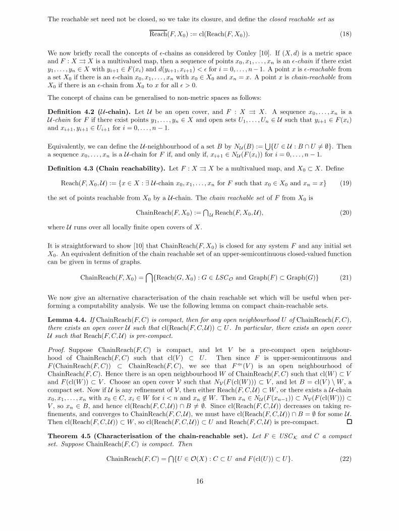
Although the representations of sets given in Section 2 are convenient for a general analysis of com-putability properties, they require an infinite amount of data. We often want to describe a set by givingan approximation using a finite amount of data. To do this, we first choose a denumerable collectionof denotable sets, which can be described exactly, and describe other sets by giving an approximatingdenotable set and an error bound. Such approximations are used in existing software for performingset-based analysis, including GAIO [11] and the ellipsoidal calculus of Kurzhanski and Valyi [15].

Figure 4: Approximations of compact sets on a grid.

A particularly important class of denotable sets in applications is that based on cuboidal grids, as shownin Figure 4. We can take a decreasing sequence of grids Gq based on the dyadic rationals Q2 := {p/2q :p ∈ Z, q ∈ N} as unions of cuboids of the form

I =[

p1

2q ,p1+12q

]×

[p2

2q ,p2+12q

]× · · · ×

[pn

2q ,pn+1

2q

](29)

21

By taking finer and finer grids, better approximations can be computed.

From a computability viewpoint, we are interested in whether it is possible to compute approximations toa set to arbitrary precision. We therefore consider approximation representations, in which we representa set by a convergent sequence of denotable sets. The advantage of approximation representations overthe standard representations is that the approximating denotable elements have the same type as theelement being represented. For real numbers, points in Euclidean space, and open and closed sets, we canfind approximation representations equivalent to the standard representations. Hence the computabilityresults for reachable and chain reachable sets in the standard representations are also valid for theapproximation representations.

We first give an outline of approximation methods in a more general setting, with the example beingthat of the real numbers and points in Euclidean space. We then consider different types of denotableclosed sets, with particular emphasis on those defined on cuboidal grids. Finally, we consider thoseapproximation representations which correspond to the standard representations ψ< of A and κ> andκ of K. The material in this section is only an introduction to the use of approximation methods; acomplete treatment is beyond the scope of this paper.

5.1 Approximation representations

We first define a general framework for considering approximations.

Definition 5.1 (Denotable element). Let (X, τ) be a second-countable Hausdorff space, and ξ :⊂Σ∗ → X be a function whose range is a dense subset of X . We say an element x ∈ X is denotable ifx = ξ(w) for some w ∈ dom(ξ). The triple (X, τ, ξ) is a denotable topological space.

Appropriate choices for denotable real numbers are the rationals Q or the dyadic rationals Q2. Appro-priate choices for denotable points in Euclidean space Rn are Qn and Qn

2 .

We can now define representations of elements of X by convergent sequences.

Definition 5.2 (Approximation representation). Let (X, τ, ξ) be a denotable topological space. Anapproximation representation of (X, τ, ξ) is a function δ :⊂ Σω → X such that

δ〈w1, w2, . . .〉 = x :⇐⇒ 〈w1, w2, . . .〉 ∈ dom(δ) and limi→∞ ξ(wi) = x. (30)

In other words, an approximation representation encodes a convergent sequence of denotable elements(xi), where xi := ξ(wi).

The main difficulty when considering approximation representations is that no finite portion of a generalconvergent sequence gives any information about its limit. The main challenge is therefore to restrict thedomain of the representation δ to sequences with appropriate properties, so that meaningful approxima-tions can be extracted. We henceforth often restrict approximation representations to (strictly) increasingor decreasing sequences, or effective Cauchy sequences with d(xi, xj) 6 εi whenever j > i, where (εi) isa strictly decreasing sequence of rationals with limi→∞ εi = 0, a typical choice being εi = 2−i

Many of the representations of real numbers R given in [23, Section 4.1] are approximation representations,most notably the Cauchy representation ρC given by

ρC〈w1, w2, . . .〉 = x :⇐⇒ |ξ(wi) − ξ(wj)| 6 2−i for i < j and x = limi→∞ ξ(wi).

The Cauchy representation is an approximation representation with domain given by

〈w1, w2, . . .〉 ∈ dom(ρC) :⇐⇒ xi := ξ(wi) satisfy |xi − xj | < 2−i for i < j.

The Cauchy representation is equivalent to the standard representation ρ. An alternative approximationrepresentation of R which is equivalent to ρ is that by alternating sequences (xi) satisfying x2i < x2i+2 <x2i+3 < x2i+1 for all i.

22

An approximation representation equivalent to the standard representation ρn of Rn is given by takingstrongly convergent sequences, where ||x − xi|| < 2−ii for all i. Here, the most natural norm to take isthe sup-norm || · ||∞.

From an approximation representation, we often wish to derive a single approximation to the representedelement. We can specify an approximation by giving an approximating denotable element, and specifyingthe type of approximation.

Definition 5.3 (Approximation). An approximation type is a function e : range(ξ) → τ . An approxi-mation to an element x ∈ X is a pair (x, e), where x is a denotable element, and e is an approximationtype, such that x ∈ e(x). We say that x is an e-approximation to x.

A lower approximation of a real number is specified by the approximation type e<(x) = (x,∞), since xis a lower approximation to x if x < x, which is equivalent to x ∈ (x,∞). An upper approximation isspecified by e>(x) = (−∞, x). An ε-approximation is specified by eε(x) = (x−ε, x+ε). ε-approximationscan be extracted from effective Cauchy sequences, since if (xi) is an effective Cauchy sequence convergingto x, then |x− xi| 6 εi for all i.

The concept of lower approximation generalises to any partially ordered topological space, and that ofε-approximation to any metric space. For general topological spaces, we can define approximations interms of an open cover. A U-approximation is specified by eU (x) =

⋃{U ∈ U : x ∈ U}, so x is a

U-approximation to x if there exists U ∈ U such that x, x ∈ U .

5.2 Approximations of sets

We now consider approximation representations of closed and compact sets. Let (X, τ, β, ν) be a com-putable Hausdorff space. Then the topological spaces (A(X), τA), (O(X), τO) and (K(X), τK) are second-countable Hausdorff spaces. An appropriate notion of a denotable set is one which can be written as afinite union of basic (open or closed) sets of X .

Definition 5.4 (Denotable set).

1. A closed set A is denotable if there are finitely many basic closed sets I1, . . . , Ik such that A =⋃k

i=1 I i. The function ν :⊂ Σ∗ → A(X) defined by

ν〈w1, . . . , wk〉 :=⋃k

i=1 ν(wi) = cl(ν〈w1, . . . , wk〉). (31)

is a notation for the denotable closed sets.

2. An open set U is denotable if there are finitely many basic open sets J1, . . . , Jk such that U =⋃k

i=1 Ji. The function ν :⊂ Σ∗ → O(X) defined by

ν〈w1, . . . , wk〉 :=⋃k

i=1 ν(wi) (32)

is a notation for the denotable open sets.

3. Since the denotable closed sets are compact, compact set C is denotable if it is a denotable closedset, C =

⋃k

i=1 I i.

There are a number of useful approximation representations of open, closed and compact sets, each basedon a type of sequence.

Definition 5.5 (Monotonic sequences). A sequence of open sets (Ui) is increasing if Ui ⊂ Uj wheneveri < j, and strictly increasing if cl(Ui) ⊂ Uj . A sequence of compact sets (Ci) is decreasing if Cj ⊂ Ci

whenever i < j, and strictly decreasing if Cj ⊂ int(Ci).

23

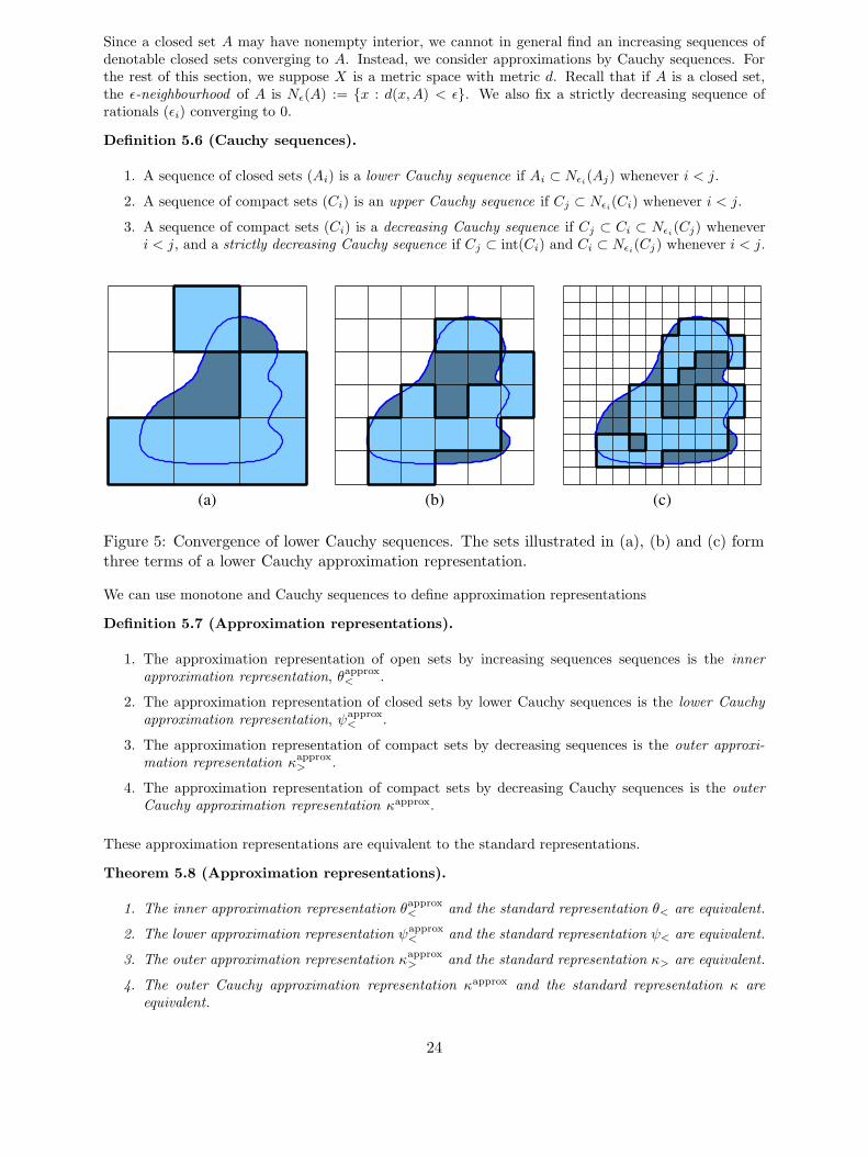
Since a closed set A may have nonempty interior, we cannot in general find an increasing sequences ofdenotable closed sets converging to A. Instead, we consider approximations by Cauchy sequences. Forthe rest of this section, we suppose X is a metric space with metric d. Recall that if A is a closed set,the ε-neighbourhood of A is Nε(A) := {x : d(x,A) < ε}. We also fix a strictly decreasing sequence ofrationals (εi) converging to 0.

Definition 5.6 (Cauchy sequences).

1. A sequence of closed sets (Ai) is a lower Cauchy sequence if Ai ⊂ Nεi(Aj) whenever i < j.

2. A sequence of compact sets (Ci) is an upper Cauchy sequence if Cj ⊂ Nεi(Ci) whenever i < j.

3. A sequence of compact sets (Ci) is a decreasing Cauchy sequence if Cj ⊂ Ci ⊂ Nεi(Cj) whenever

i < j, and a strictly decreasing Cauchy sequence if Cj ⊂ int(Ci) and Ci ⊂ Nεi(Cj) whenever i < j.

(a) (b) (c)

Figure 5: Convergence of lower Cauchy sequences. The sets illustrated in (a), (b) and (c) formthree terms of a lower Cauchy approximation representation.

We can use monotone and Cauchy sequences to define approximation representations

Definition 5.7 (Approximation representations).

1. The approximation representation of open sets by increasing sequences sequences is the innerapproximation representation, θapprox

< .

2. The approximation representation of closed sets by lower Cauchy sequences is the lower Cauchyapproximation representation, ψapprox

< .

3. The approximation representation of compact sets by decreasing sequences is the outer approxi-mation representation κapprox

> .

4. The approximation representation of compact sets by decreasing Cauchy sequences is the outerCauchy approximation representation κapprox.

These approximation representations are equivalent to the standard representations.

Theorem 5.8 (Approximation representations).

1. The inner approximation representation θapprox< and the standard representation θ< are equivalent.

2. The lower approximation representation ψapprox< and the standard representation ψ< are equivalent.

3. The outer approximation representation κapprox> and the standard representation κ> are equivalent.

4. The outer Cauchy approximation representation κapprox and the standard representation κ areequivalent.

24

(sketch).

1. Let (I1, I2, . . .) encode a θ<-name for an open set U . Then the sequence (Ui) defined by Ui :=⋃k

i=1

is an increasing sequence converging to U .

Conversely, given an increasing sequence of denotable sets (Ui) converging to U , we output I ifI ⊂ U (covering).

2. Let (J1, J2, . . .) encode a ψ<-name for a closed set A. For simplicity, we only consider the casewhere A is compact. We let Aj,k = cl(

⋃{Jm : m 6 k and diam(Jm) < εj}). We take the jth

approximation Aj = Aj,k whenever Ai,k ⊂ Nεi(Aj,k) for all i < j. The resulting sequence is a

lower Cauchy sequence converging to A.

Conversely, given a lower Cauchy sequence (Ai) converging to A, we have that Ai ⊂ cl(Nεi(A)) for

all i. Hence if J contains a basic closed set I such that I ∩ Ai 6= ∅ and cl(Nεi(I)) ⊂ J for some i,

then J ∩ A 6= ∅. If J ∩ A 6= ∅, then there exists I with I ⊂ J , and I ∩ A 6= ∅. There exists i suchthat I ∩ Ai 6= ∅ (by convergence) and cl(Nεi

(I)) ⊂ J . Hence J is output.

3. We use the representation κcv> . Given a sequence of all open covers Ui of containing C, we can take

(Ci) to be a subsequence of⋃{I : I ∈ Ui}. Given a decreasing sequence (Ci) converging to C, we

can take all open covers of the Ci to obtain all open covers of C.

4. For any i, we compute Ci such that C ⊂ int(Ci) and Ci ⊂ Nεi(C). The construction is that of [23,

page 127]. Then if i < j, we have Cj ⊂ Nεi(C) ⊂ Nεi

(Cj). By taking a subsequence if necessary,we obtain Cj ⊂ Ci for i < j.

As usual, the approximating sequences give rise to approximation concepts. A ε-lower approximation toa closed set A is a denotable closed set A such that A ⊂ Nε(A). An outer approximation to a compact

set C is a denotable compact set C such that C ⊂ C , and a strict outer approximation is a denotablecompact set C such that C ⊂ int(C). An outer ε-approximation to a compact set C is a denotable

compact set C such that C ⊂ C ⊂ Nε(C).

5.3 Approximations on grids

A natural way of approximating a compact set in Euclidean space is to construct a grid of closed cuboidswith disjoint interiors, and to take denotable sets which are a union of finitely many cuboids, as shownpreviously in Figure 4. This notion generalises to arbitrary computable Hausdorff spaces.

Definition 5.9 (Grid). A grid is a collection G of basic closed sets I such that X =⋃G and I ∩ J = ∅

whenever I, J ∈ G.

Similarly to refinements of open covers, we can consider refinements of grids. However, refinements ofgrids are more restricted, since we require that each element of the larger grid be a union of elements ofthe refinement.

Definition 5.10 (Proper refinement). A proper refinement of a grid G1 is a grid G2 such that for everyI2 ∈ G2, there exists I1 ∈ G1 such that I2 ⊂ I1, and for every I1 ∈ G1, we have I1 =

⋃{I2 ∈ G2 : I2 ⊂ I1}.

We would like to construct approximations to a compact set C as finite unions of grid elements. Clearlythe best such outer approximation on a given grid is CG :=

⋃{I ∈ G : I ∩ C 6= ∅}. Unfortunately this

concept cannot be directly effectivised, since although we can use ψ< to show I ∩C 6= ∅, and κ> to showI ∩ C = ∅, we cannot effectively decide whether C intersects the boundary of I .

To overcome this difficulty, we consider a neighbourhood N(I) for each grid element I . Assuming thatN(I) is a basic open set for every grid element I , we define a function

η :⊂ Σ∗ → Σ∗, ν(η(w)) := N(ν(w)), (33)

25

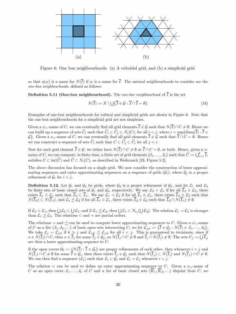
(a) (b)

Figure 6: One box neighbourhoods. (a) A cuboidal grid, and (b) a simplicial grid.

so that η(w) is a name for N(I) if w is a name for I . The natural neighbourhoods to consider are theone-box neighbourhoods, defined as follows:

Definition 5.11 (One-box neighbourhood). The one-box neighbourhood of I is the set

N(I) := X \⋃{J ∈ G : J ∩ I = ∅}. (34)

Examples of one-box neighbourhoods for cubical and simplicial grids are shown in Figure 6. Note thatthe one-box neighbourhoods for a simplicial grid are not simplexes.

Given a ψ<-name of C, we can eventually find all grid elements I ∈ G such that N(I)∩C 6= ∅. Hence we

can build up a sequence of sets Ci such that Ci ⊂ Cj ⊂ Nε(C), for all i < j, where ε = sup{diam(I) : I ∈G}. Given a κ>-name of C, we can eventually find all grid elements I ∈ G such that I ∩ C = ∅. Hence

we can construct a sequence of sets Ci such that C ⊂ Cj ⊂ Ci for all j < i.

Now for each grid element I ∈ G, we either have N(I) ∩ C 6= ∅ or I ∩ C = ∅, or both. Hence, given a κ-

name of C, we can compute, in finite time, a finite set of grid elements {I1, . . . , Ik} such that C :=⋃k

i=1 I i

satisfies C ⊂ int(C) and C ⊂ Nε(C), as described in Weihrauch [23, Figure 5.2].

The above discussion has focused on a single grid. We now consider the construction of lower approxi-mating sequences and outer approximating sequences on a sequence of grids (Gi), where Gj is a properrefinement of Gi for i < j.

Definition 5.12. Let G1 and G2 be grids, where G2 is a proper refinement of G1, and let L1 and L2

be finite sets of basic closed sets of G1 and G2, respectively. We say L2 < L1 if for all L2 ∈ L2, thereexists L1 ∈ L1 such that L2 ⊂ L1. We say L1 ≺ L2 if for all L1 ∈ L1, there exists L2 ∈ L2 such thatN(L2) ⊂ N(L1), and L1 - L2 if for all L1 ∈ L1, there exists L2 ∈ L2 such that L2 ∩N(L1) 6= ∅.

If L2 < L1, then⋃L2 ⊂

⋃L1, and if L1 - L2, then

⋃L1 ⊂ Nε1(

⋃L2). The relation L1 ≺ L2 is stronger

than L1 - L2. The relations < and ≺ are partial orders.

The relations ≺ and - can be used to compute lower approximating sequences to C. Given a ψ<-nameof C as a list (J1, J2, . . .) of basic open sets intersecting C, we let Lj,k := {I ∈ Gj : N(I) ∈ J1, . . . , Jk}.We take Lj = Lj,k if k > j and Li,k - Lj,k for all i < j. This is guaranteed to terminate, since ifx ∈ N(I i) ∩ C, then x ∈ Ij for some Ij ∈ Gj , so N(Ij ∩ C 6= ∅ and Ij ∩N(I i) 6= ∅. The sets Cj :=

⋃Lj

are then a lower approximating sequence to C.

If the open covers Ui := {N(I) : I ∈ Gi} are proper refinements of each other, then whenever i < j andN(I i) ∩ C 6= ∅ for some I ∈ Gi, then there exists Ij ∈ Gj such that N(Ij) ⊂ N(I i) and N(Ij) ∩ C 6= ∅.We can then find a sequence (Li) such that Li ⊂ Gi and Li ≺ Lj whenever i < j.

The relation < can be used to define an outer approximating sequence to C. Given a κ>-name ofC as an open cover J1, . . . , Jk of C and a list of basic closed sets (K1,K2, . . .) disjoint from C, we

26

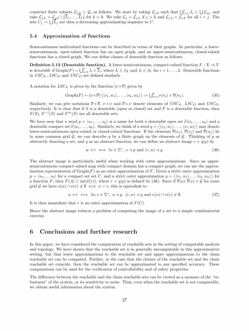
construct finite subsets Lj,k ⊂ Gj as follows. We start by taking Lj,0 such that⋃j

i=1 Ji ⊂⋃Lj0 , and

take Lj,k = Lj,0 \ {I1, . . . , Ik} for k > 0. We take Lj = Lj,k if j > k and Lj,k < Li,k for all i < j. Thesets Cj :=

⋃Lj are then a decreasing approximating sequence to C.

5.4 Approximation of functions

Semicontinuous multivalued functions can be described in terms of their graphs. In particular, a lower-semicontinuous, open-valued function has an open graph, and an upper-semicontinuous, closed-valuedfunctions has a closed graph. We can define classes of denotable function as follows.

Definition 5.13 (Denotable function). A lower-semicontinuous, compact-valued function F : X ⇒ Y

is denotable if Graph(F ) =⋃k

i=1 Ii ×J i, where Ii ∈ βX and Ji ∈ βY for i = 1, . . . , k. Denotable functionsin USCK, LSCO and USCO are defined similarly.

A notation for LSCK is given by the function (ν×ν) given by

Graph(F ) = (ν×ν)⟨〈v1, w1〉, . . . , 〈vk , wk〉

⟩:=

⋃k

i=1 ν(vi) × ν(wi). (35)

Similarly, we can give notations ν×ν, ν×ν and ν×ν denote elements of USCK, LSCO and USCO,respectively. It is clear that if S is a denotable (open or closed) set and F is a denotable function, thenF (S), F−1(S) and F⇐(S) are all denotable sets.

We have seen that a word p = 〈u1, . . . , uk〉 is a name for both a denotable open set ν〈u1, . . . , uk〉 and adenotable compact set ν〈u1, . . . , uk〉. Similarly, we think of a word q =

⟨〈v1, w1〉, . . . , 〈vl, wl〉

⟩may denote

lower-semicontinuous open-valued or closed-valued functions. If the elements ν(ui), ν(vj) and ν(wj) liein some common grid G, we can describe q by a finite graph on the elements of G. Thinking of p asabstractly denoting a set, and q as an abstract function, we can define an abstract image r = q(p) by

w � r ⇐⇒ ∃v ∈ Σ∗, v � p and 〈v, w〉 � q. (36)

The abstract image is particularly useful when working with outer approximations. Since an upper-semicontinuous compact-valued map with compact domain has a compact graph, we can use the approx-imation representation of Graph(F ) as an outer approximation of F . Given a strict outer approximationp = 〈u1, . . . ul〉 for a compact set set C, and a strict outer approximation q =

⟨〈v1, w1〉, . . . 〈vk, wk〉

⟩for

a function F , then F (A) ⊂ int(ν(r)), where r = q(p) is defined by (36). Since if ν(u), ν(v) ∈ G for somegrid G we have ν(u) ∩ ν(v) 6= ∅ ⇐⇒ u = v, this is equivalent to

w � r ⇐⇒ ∃u, v ∈ Σ∗, u� p, 〈v, w〉 � q and ν(u) ∩ ν(v) 6= ∅. (37)

It is then immediate that r is an outer approximation of F (C).

Hence the abstract image reduces a problem of computing the image of a set to a simple combinatorialexercise.

6 Conclusions and further research

In this paper, we have considered the computation of reachable sets in the setting of computable analysisand topology. We have shown that the reachable set is in generally uncomputable in this approximativesetting, but that lower approximations to the reachable set and upper approximations to the chainreachable set can be computed. Further, in the case that the closure of the reachable set and the chainreachable set coincide, then the reachable set can be approximated to any specified accuracy. Thesecomputations can be used for the verification of controllability and of safety properties.

The difference between the reachable and the chain reachable sets can be viewed as a measure of the “ro-bustness” of the system, or its sensitivity to noise. Thus, even when the reachable set is not computable,we obtain useful information about the system.

27

The type-two effectivity theory used has a number of features which we believe make it the most ap-propriate theory for the analysis of system properties. It provides a formal model of computation whichcan be realised on digital computers, and hence algorithms expressed in this theory can be practicallyrealised. There is already considerable material on the representation of open, closed and compact setsand continuous functions in this theory. The theory deals with quite general topological spaces, allowingcomputations on manifolds as well as Euclidean spaces, and also allows for the study of semicontinuousmultivalued maps and differential inclusions. As well as providing a framework for representing the stan-dard objects of topology and analysis, and for computing approximations, it also allows us to deduce thatcertain computations are not possible, simply by showing that they attempt to compute a discontinuousfunction.

Given the power of the type-two effectivity theory, the results in this paper barely scratch the surface ofwhat we believe can be achieved. We now give some possible directions for future work.

The results presented here have mostly been developed for discrete-time systems, though we have alsopresented results for continuous-time systems. We would like to extend the results further to deal withhybrid-time systems, in which evolution occurs in both continuous time (differential equations or in-clusions) and discrete time (reset maps). We expect much greater problems when considering hybridsystems, since here the evolution may be discontinuous even over finite time intervals.

We have only presented an analysis of reachability problems. Another area of study is that of viabilitytheory and invariant sets [4]. For a discrete-time multivalued system, a set A is viable if ∀x ∈ A,F (x) ∩ A 6= ∅. The viability kernel of a set A is the maximal viable subset of A. A set is invariant ifF (A) ⊂ A. The invariance kernel of a set A is the maximal invariant subset of A.

One promising tool for the study of viability problems is the Conley index [19], which computes isolatedinvariant sets. The Conley index requires the computation of homology groups related to the systemdynamics. Hence, it is important to study the formal computability properties of homology groups inthe setting of type-two effectivity.

It would also be interesting to develop these ideas further from a computational viewpoint into a “timedlogic of approximation”. In this thesis, fundamental notions of timed logic (e.g. until quantifiers) andtopological notions of approximation, closure and interior, should be combined to give a consistent frame-work for the approximative study of system properties [18]. Of particular interest is the complementationoperator, which takes closed sets to open sets and vice-versa, and timed unions and intersections (a unionover infinite times takes an open set to an open set, but need not respect closedness).

Acknowledgement. The author gratefully acknowledges the financial support of the European Com-mission through the project Control and Computation (IST-2001-33520) of the Program InformationSocieties and Technologies.

References

[1] Eugene Asarin and Ahmed Bouajjani. Perturbed Turing machines and hybrid systems. In Proceedings of the

Sixteenth Annual IEEE Symposium on Logic in Computer Science. IEEE, 2001.

[2] Eugene Asarin, Theo Dang, and Oded Maler. d/dt: A verification tool for hybrid systems. In Proceedings

of the 40th IEEE Conference on Decision and Control, New York, 2001. IEEE Press.

[3] Eugene Asarin, Oded Maler, and Amir Pnueli. Reachability analysis of dynamical systems having piecewise-constant derivatives. Theoret. Comput. Sci., 138(1):35—65, 1995.

[4] Jean-Pierre Aubin. Viability theory. Systems & Control: Foundations & Applications. Birkhauser, Boston,1991.

[5] Jean-Pierre Aubin and Helene Frankowska. Set-valued analysis. Systems & Control: Foundations & Appli-cations. Birkhauser, Boston, 1990.

[6] Errett Bishop and Douglas Bridges. Constructive analysis. Number 279 in Grundlehren der MathematischenWissenschaften [Fundamental Principles of Mathematical Sciences]. Springer-Verlag, Berlin, 1985.

[7] Vasco Brattka. Computability over topological structures. In S. Barry Cooper and Sergei S. Goncharov,editors, Computability and models, Univ. Ser. Math., page 375. Kluwer/Plenum, New York, 2003.

28

[8] Vasco Brattka and Gero Presser. Computability on subsets of metric spaces. Theoretical Comp. Sci., 305:43–76, 2003.

[9] Pierre Cardaliaguet, Marc Quincampoix, and Patrick Saint-Pierre. Set-valued numerical analysis for optimalcontrol and differential games. In Stochastic and differential games, number 4 in Ann. Internat. Soc. Dynam.Games, pages 177–247. Birkhauser, Boston, 1999.

[10] Charles Conley. Isolated Invariant Sets and the Morse Index, volume 38 of CBMS Regional Conference Series

in Mathematics. American Mathematical Society, Providence, Rhode Island, 1978.

[11] Michael Dellnitz, Gary Froyland, and Oliver Junge. The algorithms behind GAIO-set oriented numericalmethods for dynamical systems. In Bernold Fiedler, editor, Ergodic theory, analysis, and efficient simulation

of dynamical systems, pages 145–174, 805–807. Springer, Berlin, 2001.

[12] Martin Franzle. Analysis of hybrid systems: An ounce of realism can save an infinity of states. In J. Flumand M. Rodriguez-Artalejo, editors, Computer Science Logic, number 1683 in Lecture Notes in ComputerScience, Berlin Heidelberg New York, 1999. Springer-Verlag.

[13] Martin Franzle. What will be eventually true of polynomial hybrid automata. In N. Kobayashi and B. C.Pierce, editors, Theoretical Aspects of Computer Software, number 2215 in Lecture Notes in ComputerScience, pages 340–359, Berlin Heidelberg New York, 2001. Springer-Verlag.

[14] Erwin Klein and Anthony C. Thompson. Theory of correspondences. Including applications to mathematical

economics. Canadian Mathematical Society Series of Monographs and Advanced Texts. John Wiley & Sons,New York, 1984.

[15] Alexander B. Kurzhanski and Istvan Valyi. Ellipsoidal calculus for estimation and control. Systems &Control: Foundations & Applications. Birkhauser, Boston, MA, 1997.

[16] Alexander B. Kurzhanski and Pravin Varaiya. On ellipsoidal techniques for reachability analysis. I. Externalapproximations. Optim. Methods Softw., 17(2):177–206, 2002.

[17] Alexander B. Kurzhanski and Pravin Varaiya. On ellipsoidal techniques for reachability analysis. II. Internalapproximations box-valued constraints. Optim. Methods Softw., 17(2):207–237, 2002.

[18] Zohar Manna and Amir Pnueli. The temporal logic of reactive and concurrent systems. Specification. Springer-Verlag, New York, 1992.

[19] Konstantin Mischaikow and Marian Mrozek. Conley index. In Handbook of dynamical systems, volume 2,pages 393–460. North-Holland, Amsterdam, 2002.

[20] James R. Munkres. Topology: a first course. Prentice-Hall, Inc., Englewood Cliffs, N.J., 1975.

[21] Anuj Puri, Pravin Varaiya, and Vivek Borkar. Epsilon-approximation of differential inclusions. In RajeevAlur, Thomas A. Henzinger, and Eduardo D. Sontag, editors, Hybrid Systems III, volume 1066 of LNCS,pages 362–376, Berlin, 1996. Springer.

[22] Dietmar Szolnoki. Set oriented methods for computing reachable sets and control sets. Discrete Contin.

Dyn. Syst. Ser. B, 3(3):361–382, 2003.

[23] Klaus Weihrauch. Computable analysis - An introduction. Texts in Theoretical Computer Science. Springer-Verlag, Berlin, 2000.

29