Modelling agents of change in the fluvial system

Rob Thomas

Model approaches

Model approach governed by variety of factors: what we model (e.g. behaviour of today’s landscape vs.

landscape change) scale of prediction (single event vs. evolution of a drainage

network or a mountain range) why we model (exploratory or explanatory modelling

versus specific prediction), and to an unknown extent, backgrounds and tastes of

individual modellers In a river:

Spatially and/or temporally averaged properties? e.g. Reynolds-averaging, 2-D or even 1-D flow modelling, bulk sediment transport

Or movement of individual particles or fluid units Somewhere in the middle?

Model approaches

Four options for large scale modelling (Haff 1996): integrate observable, verifiable formulas for erosion and

sediment transport over large times and distances define mid-scale spatially integrated relations, or define

modified transport laws that hold over larger time and space scales

find emergent behaviour and define new relations consistent with scale of larger features and behaviour of emergent landforms

define empirical relations at necessary scale

local physics represents details of landscape, but immense information requirements limit scale of prediction

process-based relations on a coarse scale predict landscapes at very large time and space scales, making interpretation of causal mechanisms difficult

general rules focus on summarising landscape properties with goal of exploring common elements rather than suite of mechanisms that produce any particular landscape

erosion and transport laws capable of independent parameterisation and can be applied at landscape scale, such that cause and effect can be determined

Model Approaches

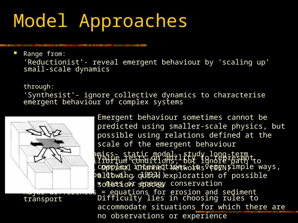
Range from:‘Reductionist’- reveal emergent behaviour by ‘scaling up’ small-scale dynamics

through:‘Synthesist’- ignore collective dynamics to characterise emergent behaviour of complex systems

to:Zero process dynamics- static model, study long-term evolution to equilibrium conditions, but ignore path to equilibrium (e.g. Optimal Channel Networks (OCN) [Rodriguez- Iturbe et al., 1992])

Common principle = mass or energy conservation Major differences = equations for erosion and sediment transport

Emergent behaviour sometimes cannot be predicted using smaller-scale physics, but possible using relations defined at the scale of the emergent behaviour

Value rests on ability to represent complex interactions in very simple ways, allowing quick exploration of possible solution spaces

Difficulty lies in choosing rules to accommodate situations for which there are no observations or experience

We generally model in the range of scales dealt with by Newtonian physics and continuum mechanics- both have bounds of application

Small-scale phenomena can be modelled from physical theory. However as scale increases physics becomes increasingly difficult to apply because: both slow- and fast-acting geomorphological processes different mechanisms dominate change at different

scales unanticipated processes unknown initial and forcing conditions governing relations generally non-linear

Issues of scale- physical models

Simulating river hydraulics: flow structures Flow in rivers is turbulent, with strongly three-dimensional flow structures

that drive deposition and erosion eddy sizes range from extremely small up to the order of the channel dimensions bedforms also occur at variety of scales

Flow structures in rivers are extremely complex Examples from 3D simulations of flow over gravels (Lane et al., in review)downstream cross-stream vectors velocity

1 0 2 0 3 0 4 0 5 0 6 0 7 0 8 0 9 0 1 0 0 1 1 0

10

20

30

40

50

60

70

80

90

100

110

120

Governing equations

Any fluid flow is described by the Navier-Stokes equations expressing

the temporal change in momentum + the spatial change in momentum = pressure gradient force + change in momentum due to frictionin the downstream, cross stream and vertical directions

And the Continuity equation expressingthe sum of change in mass (or volume) in the downstream, cross stream and vertical directions = 0

However, these equations are too complex to solve analytically (non-linear, four independent variables)

To obtain approximate numerical solutions we need simplifications and approximations

General issues..

Presently unfeasible to solve equations over spatial or temporal scale large enough to be useful for modelling rivers

Reducing dimensionality promotes reduction in effects (e.g. turbulence and secondary circulation) explicitly dealt with, and reduction in simulation time.

Additional terms, representing turbulence and secondary circulation, introduced into 2-dimensional form of equations

Potential flow representations

Convenient when velocity is constant at the fixed points Handles flow-field distortion effectively Material interfaces not easily handled Difficult to resolve sub-grid scale features Not suited to unsteady flow ‘Artificial diffusion’ as contaminants apportioned to adjacent

cells

EULERIAN approach

Flow described by velocity, acceleration and density at

points

Domain split into small cells fixed in space for which we can obtain

algebraic equations

Potential flow representations

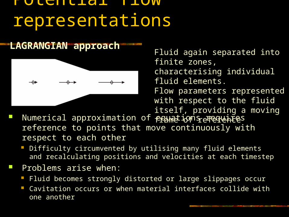
Numerical approximation of equations requires reference to points that move continuously with respect to each other Difficulty circumvented by utilising many fluid elements and

recalculating positions and velocities at each timestep

Problems arise when: Fluid becomes strongly distorted or large slippages occur Cavitation occurs or when material interfaces collide with one

another

LAGRANGIAN approachFluid again separated into finite zones, characterising individual fluid elements.Flow parameters represented with respect to the fluid itself, providing a moving frame of reference

Potential flow representations

Developed as “Particle-in-Cell” at Los Alamos in the late 1950s for use in particle physics

Adapted to fluvial hydraulics during 1980s by John Harbaugh and graduate students at Stanford

Eulerian mesh used for characterising the field variables (e.g. depth and bed elevation)

Lagrangian elements used to characterise the fluid itself (e.g. velocity and sediment load)

MARKER-IN-CELL approach

Can be considered to combine some of the best features of both Eulerian and Lagrangian approaches

Why hasn’t Marker-in-cell been used more extensively?

Advantages Disadvantages

Handles flow-field distortion Computationally demanding

Handles material interfaces Flows in which stagnations occur w.r.t Eulerian mesh are difficult to resolve

Fluid elements help resolve sub-grid scale features

Within a large region of flow there must be no small region for which detailed resolution is required

Relatively simple to deal with 2+ dimensions (fluid flow in 2-D, plus depth, logarithmic velocity profile and deposits in vertical)

It must be not be necessary to know in detail the fluid variables at Eulerian grid boundaries at any given instant of time

Potential flow rules

Flow Rules: Based on 2-D momentum equation-

Velocity = f (depth, energy slope, g, roughness)See later for sediment transport

Murray-Paola (1994, 1997)-Velocity = f (bed slope) [to some power]Sediment transport = f (bedslope · discharge)

Thomas and Nicholas (2002)-Velocity = f (bed slope, depth, g, roughness) [all raised to some power]No sediment transport

Sediment transport

Commonly, we distinguish three main transport modes:

1. dissolved load (wash load)

2. layer spanning most of water column where particles are in suspension

3. particles that roll, slide, or saltate, and are transported as bed load

Sediment transport modelling

Model approaches range from simulating: individual particles multiple size classes (split mixture into a number of

classes, each with different behaviour) single size class to ignoring it! (Sediment transport is very difficult- ask

Einstein!) Transport formulation:

suspended load bed load total load

Governing Equations

Sediment transport (in 2D) is described by the following mathematical relationship: Mass conservation of sediment by size fraction

C is depth-averaged concentration, D is particle deposition rate, E is particle entrainment rate, h is depth, t is time, U is downstream velocity, V is cross stream velocity, x is downstream distance, y is cross stream distance, s is sediment eddy diffusivity, qs is sediment inflow, and the subscript k denotes the kth size class

skkk

ks

ks

kkk qDEy

Ch

yx

Ch

xy

VhC

x

UhC

t

hC

Sediment transport modelling

Modelling of suspended load via agent-based methods largely unexplored (but wait..)

Modelling bed load more reasonable. In this case, agents would be individual particles, rolling, sliding or saltating

Rules based on: empirical functions (e.g. Laursen, Yang, Meyer-Peter and

Mueller)- some excess quantity stochastic formulations (e.g. Einstein, Shen) physical properties of particles (e.g. coefficient of restitution,

conservation of mass, momentum and energy) For example, Schmeeckle and Nelson 2003

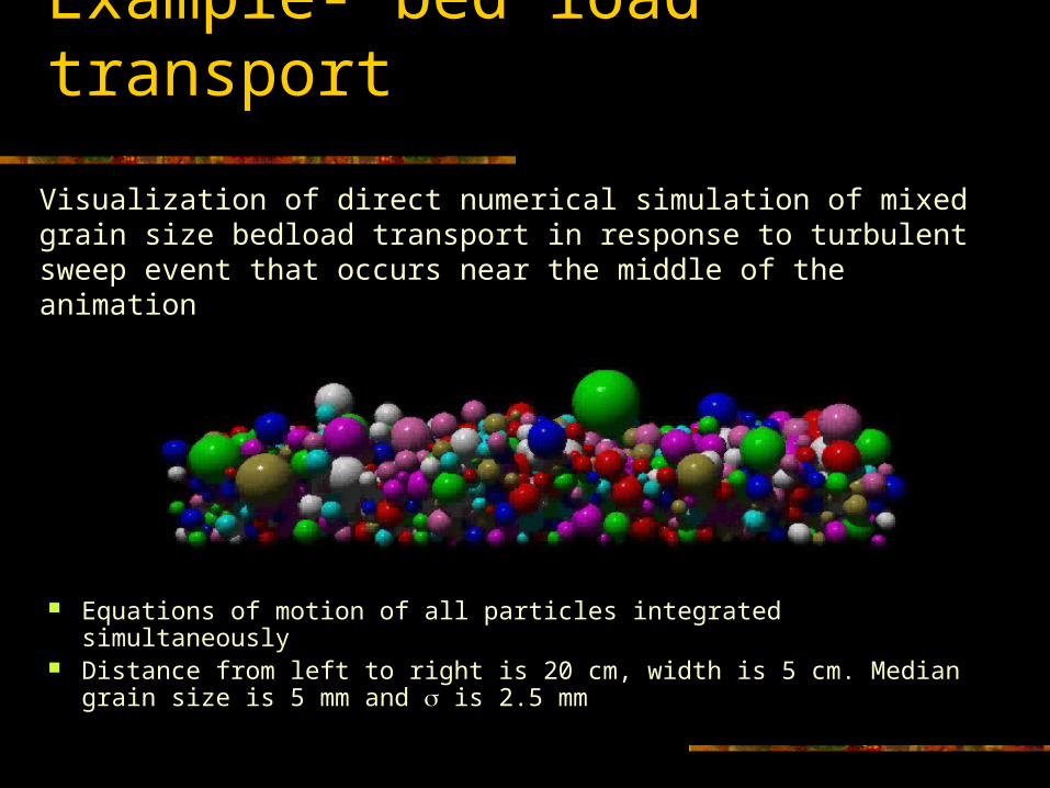
Example- bed load transport

Visualization of direct numerical simulation of mixed grain size bedload transport in response to turbulent sweep event that occurs near the middle of the animation

Equations of motion of all particles integrated simultaneously Distance from left to right is 20 cm, width is 5 cm. Median grain size is

5 mm and is 2.5 mm

SEDTRA- sediment transport capacity predictor (Garbrecht et al. 1996) Total sediment transport by

size fraction for fourteen predefined size classes with suitable transport equation for each size fraction: Wash load (particles less

than 8 m): after entrainment, not deposited

Silts and fine sands from 8 m to 0.25 mm: Laursen (1958)

Sands from 0.25 mm to 2.0 mm: Yang (1973), and

Gravels from 2.0 mm to 64.0 mm: Meyer-Peter and Mueller (1948).

Sediment transport modelling

Particles exchange between the bed- and suspended-load layers and the bed

Two options: compute sediment transport rates in each layer combine suspended and bed load layers into single total

load layer

To model sediment transport processes, three or more layers can be distinguished:•two layers through the water column, and•one or more layers covering the streambed

Summary

Range of model approaches, must be governed by application

Agents in fluvial systems- I suspect we’re already doing it, just independently

Language issues- fortran vs java Others??

Outline

Model approaches

Scale issues

Fluvial hydraulics Governing equations Difficulties Flow representations

Sediment transport Governing equations Simulation options

Issues of scale- physical models

Continuum mechanics only works well at certain scales breaks down when nonlinearity promotes localization

and “shocks,” as in breaking waves, hydraulic jumps, river channels, caves, etc.

Newtonian physics breaks down at elementary particle scale

Quantum physics- “probability functions” describing particle behaviour breaks down at even smaller scales

String theory or some yet to be invented theory

Models- What? Why?

In essence, a model is: an idealised representation of reality a description or analogy used to aid visualisation and

understanding a system of postulates, data and inferences presented as

a mathematical description of an entity or state Purposes:

organise scientific thought explore controls on landscape form and dynamics perform experiments beyond the spatial and temporal

range of observations develop understanding- “thought experiments” (cf. Kirkby)