Drug and Alcohol Information I-1183 and I-502: Updates, Impacts and Strategies for Prevention

University of Sheffield – Income group-specific impacts of alcohol minimum unit pricing in England 2014/15
1
Modelled income group-specific impacts of alcohol
minimum unit pricing in England 2014/15:
Policy appraisals using new developments to the
Sheffield Alcohol Policy Model (v2.5)
17th
July 2013
Yang Meng
Alan Brennan
John Holmes
Daniel Hill-McManus
Colin Angus
Robin Purshouse
Petra Meier
© ScHARR, University of Sheffield

University of Sheffield – Income group-specific impacts of alcohol minimum unit pricing in England 2014/15
2
Contents
Contents ............................................................................................................................................... 2
Index of Tables ................................................................................................................................... 4
Index of Figures .................................................................................................................................. 6
1 Executive summary ......................................................................................................................... 7
1.1 Main conclusions .................................................................................................................... 7
1.2 Scope of research .................................................................................................................... 7
1.3 Research Questions ................................................................................................................ 9
1.4 Summary of model findings .................................................................................................... 9
1.4.1 Patterns of drinking and expenditure ............................................................................. 9
1.4.2 Effect of minimum unit pricing on consumption and expenditure .............................. 10
1.4.3 Effects of minimum unit pricing on alcohol-related harms .......................................... 13
ACKNOWLEDGMENTS ....................................................................................................................... 17
2 Introduction .................................................................................................................................. 18
2.1 Background ........................................................................................................................... 18
2.2 Research question addressed ............................................................................................... 18
3 Methods ........................................................................................................................................ 19
3.1 New features of SAPM2.5 ..................................................................................................... 19
3.2 Overview of SAPM2.5 ........................................................................................................... 20
3.3 Modelling the link between price and consumption ............................................................ 22
3.3.1 Consumption ................................................................................................................. 23
3.3.2 Prices ............................................................................................................................. 25
3.3.3 Price elasticities of alcohol demand ............................................................................. 33
3.3.4 Price to consumption model ......................................................................................... 35
3.4 Modelling the relationship between consumption and harm .............................................. 36
3.4.1 Model structure ............................................................................................................ 36
3.4.2 Alcohol-attributable fractions and potential impact fractions ..................................... 36
3.4.3 Derivation of risk functions ........................................................................................... 38
3.5 Consumption to Health harms model ................................................................................... 41
3.5.1 Changes in SAPM2.5 model .......................................................................................... 41
3.5.2 Summary of methods unchanged since SAPM2 ........................................................... 42
3.6 Crime harms .......................................................................................................................... 48
3.6.1 Changes in SAPM2.5 model .......................................................................................... 48
3.6.2 Summary of methods unchanged since SAPM2 ........................................................... 49

University of Sheffield – Income group-specific impacts of alcohol minimum unit pricing in England 2014/15
3
3.7 Workplace harms .................................................................................................................. 50
3.7.1 Changes in SAPM2.5 model .......................................................................................... 50
3.7.2 Summary of methods unchanged since SAPM2 ........................................................... 50
3.8 Sensitivity analysis ................................................................................................................ 51
4 Results ........................................................................................................................................... 52
4.1 Summary tables for policies .................................................................................................. 52
4.2 Example policy analysis: 45p MUP (2014/15 prices) ............................................................ 63
4.3 Sensitivity analyses ............................................................................................................... 70
5 Discussion ...................................................................................................................................... 76
5.1 Comparison of results between SAPM2 and SAPM2.5 ......................................................... 76
5.2 Summary of differences between SAPM version 2.5 and previous versions. ...................... 77
5.2.1 Methodological and structural changes: ...................................................................... 77
5.2.2 Updates to underlying data: ......................................................................................... 78
5.2.3 Considerations regarding the new econometric model ............................................... 78
5.2.4 Considerations regarding the disaggregation of cider and beer .................................. 78
5.2.5 Further issues to be discussed ...................................................................................... 79
5.3 Impacts on low and higher income groups ........................................................................... 79
5.4 Impacts on revenue to retailers ............................................................................................ 80
5.5 Impacts on alcohol-related crime ......................................................................................... 81
REFERENCES ...................................................................................................................................... 82
6 Appendix ....................................................................................................................................... 85
6.1 Appendix 1: Relationship between peak daily consumption and mean daily consumption 85
6.2 Appendix 2: ONS alcohol-specific RPIs 2001 to 2011 ........................................................... 86
6.3 Appendix 3: Risk functions for health conditions ................................................................. 87
6.4 Appendix 4: Slope of relative risk functions, split by offence category and OCJS gender and
age sub-groups .................................................................................................................................. 89
6.5 Appendix 5: Slope for relative risk functions for absenteeism, split by gender and age group
90
6.6 Appendix 6: Alternative elasticity matrices used in sensitivity analyses .............................. 91
6.7 Appendix 7: Detailed results table for 45p MUP (consumption effects) for sensitivity
analyses ............................................................................................................................................. 99

University of Sheffield – Income group-specific impacts of alcohol minimum unit pricing in England 2014/15
4
Index of Tables
Table 1.1: Estimated effects on alcohol consumption .......................................................................... 11
Table 1.2: Estimated effects on consumer spending on alcohol .......................................................... 12
Table 1.3: Estimated effects on alcohol-related harms for a 45p MUP (2014/15 prices) .................... 14
Table 2.1: Matching MUP thresholds in 2014/15 prices to the model baseline year of 2011 ............. 19
Table 3.1: Summary of methodological changes .................................................................................. 20
Table 3.2: Matching of LCF/EFS product categories to modelled categories and ABV estimates. ....... 27
Table 3.3: Proportions of alcohol sold below a range of MUP thresholds ........................................... 29
Table 3.4: Proportions of LCF/EFS individuals categorised as low income ........................................... 30
Table 3.5: Comparison of average price paid and proportions of alcohol sold below 45p per unit
between two income groups ................................................................................................................ 31
Table 3.6: Comparison of average price paid and proportions of alcohol sold below 45p per unit by
moderate, hazardous and harmful drinkers (pence per unit) .............................................................. 32
Table 3.7: Estimated own- and cross-price elasticities for off- and on-trade beer, cider, wine, spirits
and RTDs in the UK ................................................................................................................................ 34
Table 3.8: Health conditions included in the model ............................................................................. 43
Table 3.9: Updated number crime volumes and costs in England ....................................................... 48
Table 4.1: Summary of estimated effects of pricing policies on alcohol consumption, spending and
sales in England ..................................................................................................................................... 53
Table 4.2: Summary of income-specific estimated effects of pricing policies on alcohol consumption,
spending and sales in England .............................................................................................................. 54
Table 4.3: Summary of male income-specific estimated effects of pricing policies on alcohol
consumption, spending and sales in England ....................................................................................... 55
Table 4.4: Summary of female income-specific estimated effects of pricing policies on alcohol
consumption, spending and sales in England ....................................................................................... 56
Table 4.5: Summary of estimated effect of pricing policies on retailer and duty/VAT revenue in
England.................................................................................................................................................. 57
Table 4.6: Summary of estimated percentage change in retailer and duty/VAT revenue in England . 57
Table 4.7: Summary of estimated effects of pricing policies on health, crime and workplace related
harm in England .................................................................................................................................... 59
Table 4.8: Summary of estimated percentage change in alcohol-attributable health, crime and
employment harms in England ............................................................................................................. 60
Table 4.9: Summary of financial valuation of impact of pricing policies on health, crime and
workplace related harm in England ...................................................................................................... 61
Table 4.10: Summary of income-specific estimated effects and financial valuation of impacts of
pricing policies on health harm related to alcohol in England ............................................................. 62
Table 4.11: Detailed results for 45p MUP (consumption and spending effects) .................................. 66
Table 4.12: Detailed income and drinker group-specific results for 45p MUP (consumption and
spending effects) ................................................................................................................................... 67
Table 4.13: Detailed male income and drinker group specific results for 45p MUP (consumption and
spending effects) ................................................................................................................................... 68
Table 4.14: Detailed female income and drinker group-specific results for 45p MUP (consumption
and spending effects) ............................................................................................................................ 69

University of Sheffield – Income group-specific impacts of alcohol minimum unit pricing in England 2014/15
5
4.15: Relative change in price for the modelled beverage types and beverage-specific impacts for
45p MUP on consumption and spending.............................................................................................. 70
Table 4.16: Probabilistic sensitivity analysis confidence interval estimates ........................................ 70
Table 4.17: Comparison of estimated impacts on alcohol consumption for a 45p MUP and a general
10% increase policy using alternative elasticities ................................................................................. 73
Table 4.18: Comparison of estimated impacts on harm reductions for a 45p MUP policy using
alternative elasticities ........................................................................................................................... 76

University of Sheffield – Income group-specific impacts of alcohol minimum unit pricing in England 2014/15
6
Index of Figures
Figure 3-1: Schematic on integrating data sources .............................................................................. 22
Figure 3-2: Distribution of mean weekly alcohol consumption among individuals in England aged 16
years old and over (GLF 2009) .............................................................................................................. 24
Figure 3-3: Distribution of peak daily intake (units drunk on heaviest drinking day in the last week)
among individuals in England aged 16 years old and over (GLF 2009) ................................................. 24
Figure 3-4: Final off-trade price distributions for beer, cider, wine, spirits and RTDs in 2011 prices .. 28
Figure 3-5: Final on-trade price distributions for beer/cider, wine, spirits and RTDs in 2011 prices ... 29
Figure 3-6: Model construction steps: creation of a new GLF and new LCF-Nielsen-CGA dataset ...... 35
Figure 3-7: Illustrative linear relative risk function for a partially attributable chronic harm (threshold
of 4 units) .............................................................................................................................................. 40
Figure 3-8: Illustrative linear absolute risk function for a wholly attributable chronic harm (threshold
of 4 units) .............................................................................................................................................. 41
Figure 3-9: Simplified mortality model structure ................................................................................. 44
Figure 3-10: Simplified structure of morbidity model .......................................................................... 46
Figure 3-11: Illustrative example of the time lag effect for chronic conditions ................................... 47
Figure 3-12: Simplified structure of crime model ................................................................................. 49
Figure 3-13: Simplified structure of workplace model ......................................................................... 51
Figure 4-1: Summary of income-specific estimated effects of MUP policies on alcohol consumption in
England.................................................................................................................................................. 57
Figure 4-2: Summary of income-specific estimated effects of MUP policies on alcohol consumption in
England.................................................................................................................................................. 58
Figure 4-3: Summary of estimated effects of MUP policies on alcohol consumption in England by
income and drinker groups ................................................................................................................... 58
Figure 4-4: Scatter plot of PSA results, showing relative change in consumption for a 45p MUP by low
income and higher income groups ....................................................................................................... 71
Figure 4-5: Scatter plot of PSA results, showing relative change in consumption for a 45p MUP by
moderate and harmful drinkers ............................................................................................................ 72
Figure 4-6: Comparison of estimated impacts on alcohol consumption of a 45p MUP policy using
alternative elasticities. .......................................................................................................................... 74
Figure 4-7: Comparison of estimated impacts on alcohol consumption of a 10% price increase policy
using alternative elasticities.................................................................................................................. 74
Figure 5-1: Comparison of estimated effects of price policies on population alcohol consumption for
different versions of SAPM. .................................................................................................................. 77

University of Sheffield – Income group-specific impacts of alcohol minimum unit pricing in England 2014/15
7
1 EXECUTIVE SUMMARY
1.1 MAIN CONCLUSIONS
Estimates from a new updated version of the Sheffield Alcohol Policy Model (version 2.5)
suggest:
1. Minimum unit pricing (MUP) policies would be effective in reducing alcohol
consumption, alcohol-related harms (including alcohol-attributable deaths,
hospitalisations, crimes and workplace absences) and the costs associated with
those harms.
2. Moderate drinkers would experience only small impacts from MUP policies.
Somewhat larger impacts would be experienced by hazardous drinkers, and the main
substantial effects would be experienced amongst harmful drinkers.
3. MUP policies would have larger impacts on low income harmful drinkers than higher
income harmful drinkers although both would be affected substantially. The impact
on low income moderate drinkers would be small in absolute terms.
1.1 BACKGROUND TO THIS REPORT
This report was produced at the request of the UK Government to inform consultation and
impact assessments around policy options for alcohol pricing arising from the publication of
The Government’s Alcohol Strategy in March 2012 [1]. Drafts of the report were provided to
the Home Office, Department of Health and HM Treasury in February and March 2013. The
substantive conclusions of the report have remained unchanged throughout this process.
An addendum to the report was produced shortly before publication in June 2013 which
provides the results of additional appraisals of the Government’s current policy of a ban on
below cost selling. Results of this analysis were also provided to the UK Government ahead
of publication.
1.2 SCOPE OF RESEARCH
This report summarises results from analyses using a new version of the Sheffield Alcohol
Policy Model (SAPM2.5) to examine the likely impact for the population of England of
introducing a minimum unit price for alcohol as proposed by the UK Government in its
Alcohol Strategy [1].
The new version builds on work previously published in 2009 using the Sheffield Alcohol
Policy Model version 2.0 (SAPM2) [2, 3]. Since 2009, the methodology that underpins SAPM

University of Sheffield – Income group-specific impacts of alcohol minimum unit pricing in England 2014/15
8
has been further developed and new data have been incorporated. The key model
developments and new data are:
How sensitive are consumers to changes in price?: New econometric modelling has
been developed to estimate price elasticities of alcohol demand using Living Cost
and Food Survey (LCF) data. In addition to using new methods for estimating price
elasticities, LCF data from 2001/2 to 2009 [4] is used (the previous model used
2001/2 to 2005/6 data). Sensitivity analyses addressing the econometric modelling
are extended and include analyses using an econometric model developed
independently by HMRC.
A specific focus on low income groups: In addition to the population being separated
into subgroups for gender, age and drinking level (moderate/hazardous/harmful1), the
population is now also categorised into low income (below the relative poverty line
defined as 60% of median equivalised household income) and higher income (i.e.
above the relative poverty line). Therefore, income-specific impacts of policy
interventions such as minimum unit pricing (MUP) can now be estimated for alcohol
consumption and alcohol-related harms to health.
The separation of cider as a distinct beverage type: cider has been separated from
beer and the 10 beverage types modelled here are off/on-trade beer, cider, wine,
spirits and ready-to-drink beverages (RTDs or alcopops).
An exclusive focus on the 16 plus age range: the revised model now focuses only on
the population aged 16 and over.
Updated to use the latest alcohol consumption data: new consumption data from the
General Lifestyle Survey (GLF) has become available for 2009 (the previous model
used 2006 data).
Updated to use the latest information on alcohol prices: The Home Office and NHS
Health Scotland have procured market research data on the overall 2011 price
distribution of off-trade and on-trade alcohol in England from The Nielsen Company
and CGA Strategy respectively. The LCF 2001/2 to 2009 data has also been used to
update model inputs on prices paid by population subgroups.
1 As in our previous analysis, we define moderate drinkers as individuals whose alcohol intake is up to
21 units per week for men or 14 units per week for women and non-drinkers are included in this group;
hazardous drinkers as between 21 and 50 units per week for men; or between 14 and 35 units for
women; and harmful drinkers as over 50 units per week for men and over 35 units for women.

University of Sheffield – Income group-specific impacts of alcohol minimum unit pricing in England 2014/15
9
Updated to use the latest information on crime: new crime volume and costs data for
2011 has been incorporated.
1.3 RESEARCH QUESTIONS
What is the estimated impact of the Government’s proposed policy of introducing a 45p
minimum price per unit of alcohol? The policy is modelled prospectively for the year 2014/15,
and 45p in 2014/15 prices is deflated back to 2011 prices for use in the model.
How would that impact vary if a lower minimum price of 40p per unit or a higher minimum
price of 50p per unit were implemented instead?
How do these impacts vary by drinker group (moderate, hazardous, harmful) and by income
group?
1.4 SUMMARY OF MODEL FINDINGS
1.4.1 Patterns of drinking and expenditure
F1. Analysis of current consumption patterns shows that harmful drinkers represent an
estimated 5.3% of the adult (16+) population of England. Specifically hazardous drinkers
make up 17.5%, moderate drinkers 61.5% and non-drinkers represent 15.7% of the
population as a whole. Non-drinkers are defined here as respondents who have not drank
alcohol in the last 12 months before the survey date. On average, moderate drinkers
consume 5.5 units per week, hazardous drinkers consume 27.2 units and harmful drinkers
consume 71.4 units.
F2. These patterns differ by income group. Just over a quarter (27.1%) of the English adult
population are classified as low income (using the definition of equivalised household
income below 60% of the population median). Non-drinking is much more common amongst
the low income group with 26.8% of those with low incomes being non-drinkers compared to
just 11.6% of those with higher incomes (p<0.001). Harmful drinking is slightly less prevalent
in the low income group (4.7% vs. 5.5%, p<0.001). Average weekly consumption is lower
among low income drinkers than higher income drinkers (12.7 vs. 14.6 units, p<0.001);
however, this pattern is not consistent across the consumption distribution. Although those
with low incomes are less likely to drink and consume less on average when they do so, low
income harmful drinkers consume more per drinker than higher income harmful drinkers. On
average, moderate drinkers with low income consume less than those with higher incomes

University of Sheffield – Income group-specific impacts of alcohol minimum unit pricing in England 2014/15
10
(4.5 vs. 5.8 units, p<0.001), hazardous drinkers consume the same in each income group
(27.2 units) but the pattern is reversed for harmful drinkers where those with low incomes
consume more on average (76.2 vs. 69.8 units, p<0.001).
F3. A MUP policy would specifically target harmful drinkers who tend to buy more of their
alcohol from the cheaper end of the price per unit distribution. Currently, moderate drinkers
purchase 12.5% of their alcohol units for less than 45p, compared to 19.5% for hazardous
drinkers and 30.5% for harmful drinkers.
F4. Low income harmful drinkers would be targeted more than higher income harmful
drinkers, although both groups would be affected. For the low income group, the proportion
of all alcohol sold below a 45p MUP threshold to moderate, hazardous and harmful drinkers
is 18.4%, 29.0% and 40.7% respectively. The equivalent figures for higher income drinkers
are 10.5%, 16.8% and 28.0%.
F5. Harmful drinkers spend a substantial amount of money on alcohol. Low income harmful
drinkers are estimated to spend £2,653 per annum and higher income harmful drinkers are
estimated to spend slightly more at £2,809 per annum. Hazardous drinkers spend less
(£1,018 for low income and £1,169 for higher income) and moderate drinkers substantially
less (£64 for low income and £302 for higher income).
F6. A substantial proportion of the alcohol sold in the off-trade (e.g. supermarkets and off-
licenses) would be affected by MUP and this differs by type of beverage. For a 45p MUP, the
proportion of off-trade sales affected for each beverage type would be 70.2% of cider, 44.8%
of beer, 38.5% of spirits, 24.9% of wine and 0.8% of RTDs. On-trade prices in bars, pubs,
clubs and restaurants would be largely unaffected, with less than 0.6% of on-trade sales
being affected.
1.4.2 Effect of minimum unit pricing on consumption and expenditure
F7. For a 45p MUP, the estimated per person reduction in alcohol consumption for the
overall population is -1.6%. In absolute terms, this equates to an annual reduction of -11.7
units per drinker per year. Increasing levels of MUP show steep increases in effectiveness in
terms of alcohol consumption reductions (40p = -1.0%, 45p = -1.6%, 50p = -2.5%).

University of Sheffield – Income group-specific impacts of alcohol minimum unit pricing in England 2014/15
11
Table 1.1: Estimated effects on alcohol consumption
Population
Low
income
Higher
income Moderate Hazardous Harmful
27.1% 72.9% 77.2% 17.5% 5.3%
15.7% 26.8% 11.6% 20.3% 0.0% 0.0%
14.1 12.7 14.6 5.5 27.2 71.4
23.2% 31.5% 20.9% 12.5% 19.5% 30.5%
MUP 40p -1.0% -2.7% -0.5% -0.3% -0.3% -2.3%
MUP 45p -1.6% -4.3% -0.9% -0.6% -0.7% -3.7%
MUP 50p -2.5% -6.2% -1.5% -1.0% -1.2% -5.4%
Price +10% -5.0% -6.0% -4.7% -4.4% -4.7% -5.8%
MUP 40p -7.2 -17.9 -3.8 -1.0 -4.8 -86.7
MUP 45p -11.7 -28.2 -6.7 -1.6 -9.5 -136.6
MUP 50p -18.2 -41.2 -11.1 -2.7 -17.3 -200.0
Price +10% -36.5 -39.9 -35.4 -12.6 -66.5 -215.1
Moderate Hazardous Harmful Moderate Hazardous Harmful
22.8% 3.1% 1.3% 54.5% 14.4% 4.0%
32.0% 0.0% 0.0% 15.5% 0.0% 0.0%
4.5 27.2 76.2 5.8 27.2 69.8
18.4% 29.0% 40.7% 10.5% 16.8% 28.0%
MUP 40p -0.9% -1.7% -4.8% -0.2% 0.0% -1.4%
MUP 45p -1.5% -2.8% -7.5% -0.3% -0.2% -2.3%
MUP 50p -2.3% -4.4% -10.6% -0.6% -0.5% -3.6%
Price +10% -5.2% -5.7% -6.9% -4.2% -4.5% -5.4%
MUP 40p -2.2 -24.1 -192.5 -0.6 -0.7 -52.8
MUP 45p -3.5 -40.0 -297.0 -1.0 -2.9 -85.2
MUP 50p -5.5 -62.4 -419.7 -1.8 -7.6 -129.7
Price +10% -12.2 -81.2 -274.8 -12.7 -63.4 -195.9
% alcohol purchased below 45p
% change per
person
Change per
drinker per year
(units)
% population
Baseline consumption (units per week per drinker)
% alcohol purchased below 45p
% non-drinkers
% population
Change per
drinker per year
(units)
% non-drinkers
% change per
person
Low income Higher income
Baseline consumption (units per week per drinker)

University of Sheffield – Income group-specific impacts of alcohol minimum unit pricing in England 2014/15
12
F8. Harmful drinkers (-3.7%) have much larger estimated consumption reductions for a 45p
MUP than hazardous (-0.7%) and moderate (-0.6%) drinkers. Low income harmful drinkers
(-7.5%) have larger consumption reductions than higher income harmful drinkers (-2.3%).
Similarly, absolute annual reductions in units consumed per drinker are much larger among
harmful drinkers (-297.0 low income, -85.2 higher income) than hazardous drinkers (-40.0
low income, -2.9 higher income) and very small for moderate drinkers (-3.5 low income, -1.0
higher income).
F9. Estimated annual reductions for other population subgroups of interest include: 16-17
year olds’ consumption falling by -0.4% (-2.5 units per year) and consumption by 18-24 year
old hazardous drinkers, falling by -1.5% (-21.4 units per year).
F10. For a 45p MUP, spending across the whole population is estimated to change by +0.4%
or +£2.60 per drinker per year. Spending increases are larger for hazardous drinkers (£9.70)
than moderate drinkers (£0.90). It is estimated that spending would slightly decrease among
harmful drinkers (-£1.70) and low income drinkers (-£1.70), but increase among higher
income drinkers (+£3.90).
Table 1.2: Estimated effects on consumer spending on alcohol
F11. For a 45p MUP, overall alcohol-related revenue to the Treasury (from duty and VAT
receipts) is estimated to change only very slightly by -£48.5m or 0.6% (-17.7m and -£30.9m
for off- and on-trade respectively). Revenue to retailers is estimated to increase by £201.1m
(+5.6%) in the off-trade and decrease by £62.2m (-0.7%) in the on-trade.
Population Low
income Higher income Moderate Hazardous Harmful
MUP 40p 0.0% -0.6% 0.2% 0.0% 0.3% -0.4% MUP 45p 0.4% -0.4% 0.6% 0.3% 0.9% -0.1% MUP 50p 1.2% 0.1% 1.4% 0.9% 1.8% 0.6% Price +10% 4.5% 3.2% 4.8% 5.4% 4.5% 3.4% MUP 40p 0.1 -2.8 1.0 0.0 3.3 -9.9 MUP 45p 2.6 -1.7 3.9 0.9 9.7 -1.7 MUP 50p 7.2 0.5 9.3 2.6 21.1 15.7 Price +10% 27.4 15.5 31.1 14.8 51.4 95.4
Moderate Hazardous Harmful Moderate Hazardous Harmful MUP 40p -0.7% -0.2% -1.2% 0.1% 0.4% -0.1% MUP 45p 0.4% 0.3% -1.4% 0.4% 1.0% 0.3% MUP 50p 2.7% 1.1% -1.5% 0.9% 2.0% 1.2% Price +10% 13.4% 3.3% 2.1% 5.6% 4.7% 3.9% MUP 40p -0.5 -2.1 -31.9 0.2 4.5 -2.9 MUP 45p 0.3 3.0 -37.4 1.1 11.2 9.7 MUP 50p 1.7 11.5 -39.9 2.8 23.2 33.5 Price +10% 8.6 33.7 55.3 16.8 55.2 108.2
% change per drinker
Change per drinker per year (£)
Higher income
% change per drinker
Change per drinker per year (£)
Low income
University of Sheffield – Income group-specific impacts of alcohol minimum unit pricing in England 2014/15
13
1.4.3 Effects of minimum unit pricing on alcohol-related harms
F12. There are substantial estimated reductions in alcohol-related harm for a 45p MUP. As a
time lag is typically observed between reductions in alcohol consumption and changes in
rates of some harms to health [5], the full impact of MUP accrues over several years. For a
45p MUP, the estimated reduction in alcohol-attributable deaths is -123 in the first year and -
624 per annum from the tenth year onwards. The majority of the reduction in alcohol-
attributable deaths is seen among harmful drinkers (554 out of 624).

University of Sheffield – Income group-specific impacts of alcohol minimum unit pricing in England 2014/15
14
Table 1.3: Estimated effects on alcohol-related harms for a 45p MUP (2014/15 prices)
Population
Low
income
Higher
income Moderate Hazardous Harmful
Deaths -123 -76 -47 -17 -21 -85
Hospital admissions ('000s) -5.7 -3.6 -2.1 -0.9 -1.0 -3.8
Deaths -624 -392 -232 -11 -60 -554
Hospital admissions ('000s) -23.7 -15.6 -8.1 -1.4 -1.8 -20.5
Total crimes ('000s) -34.2 -8.9 -10.5 -14.8
Days absent from work ('000's) -247.6 -55.8 -73.9 -117.9
Healthcare costs -417.2 -270.4 -146.9 -49.5 -58.4 -309.4
Crime costs -1,148.8 -287.9 -333.5 -527.4
Absence costs -224.8 -48.9 -64.6 -111.2
Total direct costs -1,790.8 -386.3 -456.5 -948.0
Total value of harm reduction incl. QALYs2 -3,381.9 -627.8 -683.6 -2,070.5
Cumulative
discounted
harm
reductions (£m)
(Years 1-10)
n/a1
n/a1
Year 1
Year 10: Full
effect per year
Moderate Hazardous Harmful Moderate Hazardous Harmful
Deaths -9 -16 -50 -7 -4 -35
Hospital admissions ('000s) -0.5 -0.8 -2.3 -0.4 -0.3 -1.5
Deaths -4 -68 -320 -7 8 -234
Hospital admissions ('000s) -0.9 -1.9 -12.9 -0.5 0.0 -7.7
Healthcare costs -30.5 -49.0 -190.9 -19.0 -9.3 -118.5
Total value of health harm reduction incl.
QALYs2 -182.3 -235.6 -764.5 -112.7 -56.2 -515.0
Higher income
Year 1
Year 10: Full
effect per year
Low income
Cumulative
discounted
harm
reductions (£m)
(Years 1-10)
1 Income-specific results for crime and absenteeism are not available in SAPM2.5
2 QALY: quality adjusted life years

University of Sheffield – Income group-specific impacts of alcohol minimum unit pricing in England 2014/15
15
F13. Further methodological development of the model is required to account for the extent
to which the risks associated with higher alcohol consumption are different for low income
and higher income subgroups. We have used national average risk estimates (i.e. equal
risks per unit of alcohol consumed for both income subgroups and equal baseline risks).
Therefore the estimated reductions in harms presented here for low income groups may be
under-estimated, whilst the reductions for higher income groups may be over-estimated.
With this caveat stated, larger estimated reductions in deaths per annum are seen amongst
low income drinkers (-392) compared to higher income drinkers (-232).
F14. For a 45p MUP, alcohol-attributable morbidity decreases with an estimated reduction of
-12,500 illnesses and -23,700 hospital admission per annum across all drinkers 10 years
after policy implementation.
F15. Direct costs to healthcare services are estimated to reduce with changes of -£25.3m in
year 1 and -£417.2m in total over the first ten years of the policy.
F16. Crime is estimated to fall with -34,200 fewer offences overall. Almost 43% of this
annual reduction, or 14,800 crimes, are amongst harmful drinkers and 31%, or 10,500
crimes, is amongst hazardous drinkers. Costs of crime are estimated to reduce by -£138.1m
per year.
F17. Workplace absence is estimated to fall by -247,600 days per year.
F18. For a 45p MUP, the total societal value of harm reductions for health, crime and
workplace absence is estimated at £3.4bn in total over the 10 year period modelled. In the
first year, the estimated societal value of the harm reductions is as follows: NHS direct cost
reductions (£25.3m), direct crime costs saved (£138.1m), workplace absences avoided
(£27.0m). The total discounted value of harm reductions including health quality-adjusted
life years (QALYs)2 for the first ten years of the policy is £3.4bn. The societal value of harm
reductions is distributed differentially across the drinker groups over the 10 year period with
reductions in alcohol consumption among harmful drinkers accounting for 61.2% of the total
value, hazardous drinkers 20.2% and moderate drinkers 18.6%.
F19. A range of sensitivity analyses (SA) including a probabilistic sensitivity analysis and six
alternative price elasticity estimates were performed to test the uncertainty around model
estimates. The sensitivity analyses (SA) were: SA1 and SA2 adjusted the base case
elasticity matrix; SA3 used separate elasticity matrices for low and higher income groups;
2 We valued a health QALY at £60,000 in this report to be consistent with the valuations used by the
Department of Health.

University of Sheffield – Income group-specific impacts of alcohol minimum unit pricing in England 2014/15
16
SA4 used separate elasticity matrices for moderate versus hazardous/harmful drinkers; SA5
used elasticities estimated within a time series analysis of Her Majesty’s Revenue and
Customs (HMRC) data on alcohol released for consumption or sale in the UK; SA6 used
elasticities estimated independently by Her Majesty’s Revenue and Customs (HMRC). Each
of these sensitivity analyses gives broadly similar results to the base case, which provides
marginally the lowest estimated impacts of a 45p MUP of the seven estimates made.
Population consumption reduction estimates from the sensitivity analyses range from -1.7%
to -3.1% (compared to the base case of -1.6%). Importantly, harmful drinkers are
consistently shown to be substantially more affected by a MUP than moderate drinkers and
the income group-specific effects seen in the base case are maintained across each of the
sensitivity analyses undertaken.

University of Sheffield – Income group-specific impacts of alcohol minimum unit pricing in England 2014/15
17
ACKNOWLEDGMENTS
This work was funded by the Medical Research Council and the Economic and Social
Research Council (G0000043).
The ScHARR team would like to acknowledge the following people and organisations for
advice and support during the development of this research: William Ponicki (Pacific Institute
for Research and Evaluation, US), Paul Gruenewald (Pacific Institute for Research and
Evaluation, US), Tim Stockwell (University of Victoria, Canada), Andrew Leicester (Institute
for Fiscal Studies, UK), and other members of our research team and scientific advisory
group who provided advice or other contributions during the production of this report.
The team would also like to acknowledge Home Office, Department of Health, NHS Health
Scotland and Her Majesty’s Revenue and Customs for sharing data with us for this research.
The Living Cost and Food Survey and the General Lifestyle Survey are Crown Copyright.
Neither the Office for National Statistics, Social Survey Division, nor the Data Archive,
University of Essex bears any responsibility for the analysis or interpretation of the data
described in this report.

University of Sheffield – Income group-specific impacts of alcohol minimum unit pricing in England 2014/15
18
2 INTRODUCTION
2.1 BACKGROUND
In 2009, ScHARR developed the Sheffield Alcohol Policy Model version 2.0 (SAPM2) to
appraise the potential impact of alcohol policies, including different levels of MUP, for the
population of England [2, 6]. Results from SAPM have been influential in informing the
policy debate around MUP and, in March 2012, the UK Government included a commitment
to introduce a MUP in its alcohol strategy [1, 7]. In November 2012, the Home Office
launched a public consultation addressing a range of measures proposed in the strategy
including a proposed MUP 45p per unit of alcohol (1 unit = 8g/10ml of ethanol) in 2014/15
prices [8].
Since 2009, the methodology that underpins SAPM has been further developed and new
data has become available. This research report combines the new SAPM methodology
(referred to here as SAPM2.5) with the latest data available for England to produce new
estimates of the potential effects of MUP policies in England.
2.2 RESEARCH QUESTION ADDRESSED
The set of policies analysed are MUP polices with thresholds of 40p, 45p and 50p in 2014/15
prices. We also assume that these price thresholds are held constant in real terms over the
length of the 10 year modelling period. The main research questions are concerned with the
likely effects of introducing a MUP on alcohol consumption, spending, sales, health, crime
and workplace absenteeism in England.
This analysis uses 2011 as the baseline year. Table 2.1 shows the adjusted price
thresholds, in 2011 prices for the 40p, 45p and 50p MUP thresholds in 2014/15 prices.
These estimates were provided by the Home Office by forecasting future beverage-specific
retail price indices (RPIs). Therefore, for example, when appraising the impact of a 45p MUP
policy, the actual price thresholds used as inputs to SAPM are 41.2p, 42.3p, 41.2p, 40.1p
and 41.8p for off-trade beer, cider, wine, spirits and RTDs respectively and 41.4p, 41.8p,
41.6p, 41.6p and 41.5p for on-trade beer, cider, wine, spirits and RTDs respectively.
Hereafter, references to 40p, 45p and 50p MUPs should be read as 2014/15 prices unless
otherwise specified.

University of Sheffield – Income group-specific impacts of alcohol minimum unit pricing in England 2014/15
19
Table 2.1: Matching MUP thresholds in 2014/15 prices to the model baseline year of 2011
MUP policy in 2014/15 40p MUP 45p MUP 50p MUP
2011 prices (pence)
Off-beer 36.6 41.2 45.7
Off-cider 37.6 42.3 47.0
Off-wine 36.6 41.2 45.8
Off-spirits 35.6 40.1 44.5
Off-RTDs 37.2 41.8 46.5
On-beer 36.8 41.4 46.0
On-cider 37.1 41.8 46.4
On-wine 36.9 41.6 46.2
On-spirits 36.9 41.6 46.2
On-RTDs 36.9 41.5 46.2
3 METHODS
This section outlines the methods used to appraise pricing policies within SAPM. It begins
by setting out the main changes to the structure and models parameters used in SAPM2 and
then provides a detailed description of methods used at each stage of the analysis.
3.1 NEW FEATURES OF SAPM2.5
Since the publication of results from SAPM2 in 2009, the methodology of SAPM has been
further developed. Compared with SAPM2, the revised model has the following new features:
New price elasticities of demand: A new econometric model has been developed
to estimate price elasticities of alcohol demand using a pseudo-panel analysis of the
annual Living Cost and Food Survey (LCF), previously known as the Expenditure and
Food Survey (EFS), data from 2001/2 to 2009. In addition to the methodological
change, previous analyses used pooled EFS data from 2001/2 to 2005/6.
Revised beverage categories: In the econometric model and the policy/price-to-
consumption (P2C) component of SAPM, cider is now analysed as a separate
beverage type to beer and we no longer separate high and low priced products. The
10 beverage types modelled are now off/on-trade beer, cider, wine, spirits and ready-
to-drinks (RTDs).
Income-based subgroups: In addition to the study population being separated into
subgroups of gender, age and drinking level (moderate/hazardous/harmful3), the
3 As in the previous analysis, we defined moderate drinkers as individuals whose alcohol intake is no more than
21 units per week for men or 14 units per week for women; hazardous drinkers as individuals whose alcohol intake is more than 21 but less than 50 units per week for men; more than 14 but less than 35 units for women; and harmful drinkers as individuals whose alcohol intake is more than 50 units per week for men and more than 35 units per week for women.

University of Sheffield – Income group-specific impacts of alcohol minimum unit pricing in England 2014/15
20
population is now also categorised as low income (below 60% of median equivalised
household income) or higher income. Income-category specific impacts of policy
interventions, such as MUP, can now be estimated for alcohol consumption and
alcohol-related harms4. By including two income groups, a total of 96 subgroups
(defined by gender, 8 age groups, 3 drinker groups, and 2 income groups) are
modelled in SAPM2.5.
Underage drinkers: We no longer include 11-15 year olds in SAPM2.5 due to a lack
of evidence on both consumption patterns and the relationship between consumption
and harms for this young age group. We continue to include 16 and 17 year olds as
data on these drinkers is available in the GLF.
A summary of the methodological changes is provided in Table 3.1. Within SAPM2.5, most
of the methodological developments have been to the price to consumption (P2C) model,
where the changes in alcohol consumption are estimated for price-based interventions such
as MUP. In contrast, the methodology of the consumption to harm (C2H) part of the model,
where changes in alcohol-related harms are estimated from changes in consumption, has
remained largely unchanged. For details of the original methodology of SAPM2, please refer
to our previous report [2].
Table 3.1: Summary of methodological changes
Model area Methodology change Raw data change Derived model
parameters
Model structure Yes
Prices Yes
Consumption Yes
Health harms Yes
Crime harms Yes
Absenteeism Yes
3.2 OVERVIEW OF SAPM2.5
The aim of SAPM2.5 is to appraise MUP policy options via cost-benefit analyses. We have
broken down the aims into a linked series of policy impacts to be modelled
The effect of the policy on the distribution of prices for different types of alcohol;
4 The functionality for deriving income specific impacts for alcohol-related harms has not been fully
operationalised in SAPM2.5. Although income-specific harm effects can be seen, these do not account for differential relationships between alcohol consumption and risk of harm between income groups.

University of Sheffield – Income group-specific impacts of alcohol minimum unit pricing in England 2014/15
21
The effect of changes in price distributions on patterns of both on-trade and off-trade
alcohol consumption;
The effect of changes in alcohol consumption patterns on revenue for retailers and
the exchequer;
The effect of changes in alcohol consumption patterns on consumer spending on
alcohol;
The effect of changes in alcohol consumption patterns on levels of alcohol-related
health harms;
The effect of changes in alcohol consumption patterns on levels of crime;
The effect of changes in alcohol consumption patterns on levels of workplace
absenteeism;
To estimate these effects, two connected models have been built:
1. A model of the relationship between alcohol prices and alcohol consumption which
accounts for the relationship between average weekly and peak daily consumption
and how consumption is distributed within the population. These relationships are
modelled for both the total population and for population subgroups defined by
gender, age, income and consumption level.
2. A model of the relationship between (1) average weekly and peak daily consumption
and (2) harms related to health, crime and workplace absenteeism and costs
associated with these harms.
Figure 3.1 indicates the main datasets used to provide different aspects of the picture. The
model links evidence from these datasets to enable comprehensive appraisals of the
potential impacts of a policy on a range of outcomes of interest.

University of Sheffield – Income group-specific impacts of alcohol minimum unit pricing in England 2014/15
22
Figure 3-1: Schematic on integrating data sources
3.3 MODELLING THE LINK BETWEEN PRICE AND CONSUMPTION
One major aspect in the modelling exercise was to integrate datasets on price and
consumption due to the absence of an English dataset covering both of these components.
While the GLF provides good estimates of subgroup-specific alcohol consumption patterns
in England, it does not contain information on purchasing. In particular, it provides no
information on how much was paid for alcohol consumed or whether it was purchased in the
on-trade or the off-trade. Conversely, while the LCF provides a good picture of alcohol
purchasing in England, a consumption distribution based on this dataset may not reflect
accurately patterns of consumption in England at the subgroup level, as it only covers a two
week diary period and purchasers of alcohol are not necessarily the consumers.
The link between price and consumption was thus modelled using different datasets. This
section provides an overview of the data sources on alcohol consumption and pricing which
were used, before detailing the procedures for modelling the effect of price policies on
consumption.

University of Sheffield – Income group-specific impacts of alcohol minimum unit pricing in England 2014/15
23
3.3.1 Consumption
The General Lifestyle Survey (GLF), previously known as the General Household Survey
(GHS), provides two primary measures of alcohol consumption in units for the 96 subgroups
in the model. These are typical weekly consumption over the last year (average weekly) and
consumption on the heaviest drinking day during the survey week (peak daily). Both
measures can be disaggregated into beverage types. The previous model used data from
the 2006 GHS; however data from the GLF 2009 are now available and have been used as
the new baseline data in the model.
As in previous versions of the model, the price elasticities used in SAPM 2.5 relate a change
in price to a change in mean consumption; therefore an additional step is required to
estimate the effects of a change in price on peak daily consumption. As described by
Purshouse et al,[2] this is achieved by estimating the average relationship between relative
change in mean weekly consumption and relative change in peak daily consumption at
subgroup level and using this relationship to estimate how an individual’s peak daily
consumption changes following a change in mean weekly consumption. The same
methodology is applied in this analysis and the resulting model parameters from the GLF
2009 data are shown in Appendix 1.
Figure 3.2 and 3.3 present the distributions of average weekly and peak daily alcohol
consumption for males and females in England based on the GLF 2009. Please note that
the proportion of respondents reporting zero consumption is larger for peak daily
consumption than for mean weekly consumption as it is based only on drinking in the survey
week rather than the last year.
Three consumption groups are used in SAPM 2.5; moderate drinkers who consume less
than 14 or 21 units per week for females and males respectively, hazardous drinkers who
consume 14 to 35 (females) or 21 to 50 (males) units per week and harmful drinkers who
consume more than 35 (females) or 50 (males) units per week. From the GLF 2009, 15.7%
of the adult (16+) population of England are non-drinkers, 77.2% are moderate drinkers,
17.5% are hazardous drinkers and 5.3% are harmful drinkers. On average, moderate
drinkers consume 5.5 units per week, hazardous drinkers consume 27.2 units and harmful
drinkers consume 71.4 units.

University of Sheffield – Income group-specific impacts of alcohol minimum unit pricing in England 2014/15
24
Figure 3-2: Distribution of mean weekly alcohol consumption among individuals in England aged 16 years old and over (GLF 2009)
Figure 3-3: Distribution of peak daily intake (units drunk on heaviest drinking day in the last week) among individuals in England aged 16 years old and over (GLF 2009)
0%
5%
10%
15%
20%
25%
30%
35%
40%
45%
none 0 to10
units
10 to20
units
20 to30
units
30 to40
units
40 to50
units
50 to60
units
60 to70
units
70 to80
units
80 to90
units
90 to100units
Morethan100units
Male
Female
0%
5%
10%
15%
20%
25%
30%
35%
40%
45%
50%
none 0 to 2units
2 to 4units
4 to 6units
6 to 8units
8 to10
units
10 to12
units
12 to14
units
14 to16
units
16 to18
units
18 to20
units
Morethan20
units
Male
Female

University of Sheffield – Income group-specific impacts of alcohol minimum unit pricing in England 2014/15
25
Using the income groups defined on page 30, consumption patterns vary by income groups.
Non-drinking is much more common amongst the low income group with 26.8% of those with
low incomes being non-drinkers compared to just 11.6% of those with higher incomes.
Harmful drinking is slightly less prevalent in the low income group (4.7% vs. 5.5%, p<0.001).
Average weekly consumption is lower among low income drinkers than higher income
drinkers (12.7 vs. 14.6 units, p<0.001); however, this pattern is not consistent across the
consumption distribution. Although those with low incomes are less likely to drink and
consume less on average when they do so, low income harmful drinkers consume more per
drinker than higher income harmful drinkers. On average, moderate drinkers with low income
consume less than those with higher incomes (4.5 vs. 5.8 units, p<0.001), hazardous
drinkers consume the same in each income groups (27.2 units) but the pattern is reversed
for harmful drinkers where those with low incomes consume more on average (76.2 vs. 69.8
units, p<0.001).
3.3.2 Prices
In SAPM2 [2], the separate on-trade and off-trade price distributions for beer and cider
(combined), wine, spirits and RTDs were based on English purchasing data from the EFS
2001/2 to 2005/6. These were then adjusted at the population level to match England and
Wales sales data from the Nielsen Company and England-only data from CGA Strategy[9,
10]. The methods for constructing these distributions are described below. In brief, we have
used nine years of LCF data (converted to price per unit and inflated to 2011 prices) to build
ten detailed price distributions for beer, cider, wine, spirits and RTDs in both the off- and on-
trade. We then adjusted the LCF data to align with the more aggregated (but more accurate),
sales data from Nielsen and CGA to ensure that the price distribution matches with actual
sales data at known points of the distribution. The LCF data were then interpolated between
the known Nielsen and CGA data points and the resulting combined price distributions were
disaggregated into the different gender, age, income and drinking level sub-populations (e.g.
18-24 year old, male, low income, hazardous drinkers) using the demographic data in the
LCF.
LCF/EFS data is now available from 2001/2 to 2009. As in the original model, individual-level
quantities of alcohol purchased are not available in the standard version of the dataset held
by the UK Data Archive. However, via a special data request to the Department for
Environment, Food and Rural Affairs (DEFRA), anonymised individual-level diary data on 25
categories of alcohol (e.g., off-trade beers, see Table 3.3 for a complete list) detailing both
expenditure (in pence) and quantity (in natural volume of product) were made available to

University of Sheffield – Income group-specific impacts of alcohol minimum unit pricing in England 2014/15
26
the authors. Therefore, in this analysis, England transaction data from the LCF/EFS 2001/2
to 2009 is used with a total sample size of 227,933 purchasing transactions. These
transactions were used for constructing the baseline empirical price distributions for each
modelled subgroup and each modelled beverage type (i.e. 960 empirical price distributions
in total, with an average sample size of around 220 observations per distribution).
Table 3.2 also shows the matching of the LCF/EFS categories and the 10 modelled
categories and the alcohol by volume (ABV) estimates used in the LCF 2009 for converting
the natural volume of beverages to ethanol contents.
Off-trade price distributions based on aggregated sales data were compiled by the Nielsen
Company for England and Wales in 2011 for beer, cider, wine, spirits and RTDs. These
were made available to the authors be NHS Health Scotland [11] and were used to adjust
the LCF/EFS off-trade prices using the same methodology as in the original model [2]. The
Nielsen company is unable to estimate off-trade sales by Aldi and Lidl from September 2011,
and therefore the off-trade price distributions for 2011 are based on off-trade sales excluding
these stores [11]. The impact of excluding Aldi and Lidl on off-trade price distributions in
Scotland using 2009 and 2010 data was examined and only a marginal impact on the overall
off-trade price distribution was detected [11].

University of Sheffield – Income group-specific impacts of alcohol minimum unit pricing in England 2014/15
27
Table 3.2: Matching of LCF/EFS product categories to modelled categories and ABV estimates.
LCF/EFS
off/on trade
LCF/EFS category Modelled
category
ABV
estimate
Off-trade Beers off-trade beer 3.9%
Off-trade Lagers and continental beers off-trade beer 3.9%
Off-trade Ciders and perry off-trade cider 4.8%
Off-trade Champagne, sparkling wines and wine with
mixer
off-trade wine 11.2%
Off-trade Table wine off-trade wine 12.7%
Off-trade Spirits with mixer off-trade spirits 7.3%
Off-trade Fortified wines off-trade wine 14.3%
Off-trade Spirits off-trade spirits 39.6%
Off-trade Liqueurs and cocktails off-trade spirits 33.3%
Off-trade Alcopops off-trade RTD 4.6%
On-trade Spirits on-trade spirits 41.8%
On-trade Liqueurs on-trade spirits 29.9%
On-trade Cocktails on-trade spirits 13.2%
On-trade Spirits or liqueurs with mixer on-trade spirits 7.7%
On-trade Wine (not sparkling) including unspecified 'wine' on-trade wine 11.1%
On-trade Sparkling wines and wine with mixer (e.g.
Bucks Fizz)
on-trade wine 9.5%
On-trade Fortified wine on-trade wine 17.3%
On-trade Cider or perry - half pint or bottle on-trade cider 4.8%
On-trade Cider or perry - pint or can or size not specified on-trade cider 4.8%
On-trade Alcoholic soft drinks (alcopops), and ready-
mixed bottled drinks
on-trade RTDs 4.6%
On-trade Bitter - half pint or bottle on-trade beer 4.3%
On-trade Bitter - pint or can or size not specified on-trade beer 4.3%
On-trade Lager or other beers including unspecified
'beer' - half pint or bottle
on-trade beer 5.0%
On-trade Lager or other beers including unspecified
'beer' - pint or can or size not specified
on-trade beer 5.0%
On-trade Round of drinks, alcohol not otherwise specified on-trade beer 4.8%

University of Sheffield – Income group-specific impacts of alcohol minimum unit pricing in England 2014/15
28
Updated CGA Strategy data has also become available for England and Wales in 2011 for
beer/cider, wine, spirits and RTDs and this was used to adjust the LCF/EFS on-trade prices.
The CGA data was purchased by the Home Office and, although the detailed dataset is not
publicly available, the University of Sheffield is permitted to use the data for updating SAPM.
Alcohol-specific RPIs for off- and on-trade beer and off- and on-trade wine and spirits (see
Appendix 2) were used to adjust to 2011 prices the data in the LCF/EFS 2001/2 to 2009.
The 2011 price could then be aligned with the more accurate but more aggregated sales
data from the Nielsen Company data and CGA strategy data using the same methods
employed in previous versions of SAPM [6]. All final off- and on-trade price distributions
used in SAPM2.5 are in 2011 prices and are calculated for England only. The baseline year
of 2011 is chosen for the model because the latest available Nielsen and CGA price data is
based on that year. The final England aggregate price distributions for off- and on-trade beer,
cider wine, spirits and RTDs in 2011 prices used in the model are shown in Figure 3.4,
Figure 3.5 and the proportions of each beverage category sold below different MUP
thresholds in 2014/15 prices are shown in Table 3.3.
Figure 3-4: Final off-trade price distributions for beer, cider, wine, spirits and RTDs in 2011 prices

University of Sheffield – Income group-specific impacts of alcohol minimum unit pricing in England 2014/15
29
Figure 3-5: Final on-trade price distributions for beer/cider, wine, spirits and RTDs in 2011 prices
Table 3.3: Proportions of alcohol sold below a range of MUP thresholds
Proportions sold below thresholds (2014/15 prices)
40p 45p 50p
Off-trade beer 29.4% 44.8% 59.5%
Off-trade cider 59.8% 70.2% 77.3%
Off-trade wine 10.7% 24.9% 41.2%
Off-trade spirits 13.1% 38.5% 59.8%
Off-trade RTDs 0.2% 0.8% 1.6%
On-trade beer 0.0% 0.2% 0.4%
On-trade cider 0.0% 0.0% 0.3%
On-trade wine 0.4% 0.6% 1.2%
On-trade spirits 0.1% 0.1% 0.1%
On-trade RTDs 0.0% 0.0% 0.1%
0%
20%
40%
60%
80%
100%
0.20 0.40 0.60 0.80 1.00 1.20 1.40 1.60 1.80 2.00 2.20 2.40
Price (£/unit)
On-trade price distributions (2011 prices)
On-trade beer On-trade cider On-trade wine On-trade spirits On-trade RTDs

University of Sheffield – Income group-specific impacts of alcohol minimum unit pricing in England 2014/15
30
Although SAPM works on subgroup-specific price distributions, the figures and table provide
approximations of the overall proportion of alcohol within each category that would be
directly affected by MUP policies. It is apparent that these policies have a minimal impact on
on-trade prices and mainly target off-trade prices; especially prices for off-trade cider, beer
and spirits. For example, a 45p MUP defined in 2014/15 prices would affect around 70.2% of
cider sales, 44.8% of beer, 38.5% of spirits, 24.9% of wine and 0.8% of RTDs in the off-trade
and <0.6% of on-trade sales.
In SAPM2.5, apart from gender, age group and drinker group, individuals in the LCF/EFS
are categorised as low income (below 60% of median equivalised household income) or
higher income bracket (above this threshold) to construct subgroup-specific price
distributions. The threshold used is the standard definition of relative poverty in the UK and
this definition uses equivalised household income to account for differences in levels of
disposable income based on household composition. Table 3.4 shows the proportions of
individuals categorised as low income in each LCF/EFS survey based on the equivalised
household income variables recorded in these surveys.
Table 3.4: Proportions of LCF/EFS individuals categorised as low income
Table 3.5 compares the average price per unit paid and the proportions of alcohol sold
below 45p per unit for 10 modelled beverage types and for low and higher income drinkers.
It shows that low income drinkers pay around 14.9% (ranging from 5.1% to 17.1%) less than
higher income drinkers per unit of alcohol. Compared to higher income drinkers, low income
drinkers have higher proportions of alcohol sold below modelled MUP thresholds for most
beverage types. For example, while 44.8% of off-trade beer sold is below 45p per unit for the
England population (see Table 3.3), the proportions are 50.1% and 43.1% for low- and
higher income drinkers respectively (Table 3.5). For all alcohol sold (off- and on-trade), the
proportions sold below a 45p MUP threshold are 31.5% and 20.9% for low- and higher
Year Low income (%)
2001 23.5%
2002 23.3%
2003 19.6%
2004 19.2%
2005 19.7%
2006 22.0%
2007 21.5%
2008 19.8%
2009 20.1%
Total 21.5%

University of Sheffield – Income group-specific impacts of alcohol minimum unit pricing in England 2014/15
31
income drinkers. The data indicates that low income drinkers will be more affected by MUP
polices than higher income drinkers.
Table 3.5: Comparison of average price paid and proportions of alcohol sold below 45p per unit between two income groups
Average price paid in pence per unit (2011 prices)
Proportion of purchases below 45p per unit (2014/15 prices)
Low income
Higher income
% difference Low income Higher income
Off-trade beer 42.9 45.2 5.1% 50.1% 43.1%
Off-trade cider 33.6 39.9 15.9% 78.3% 66.2%
Off-trade wine 47.8 55.3 13.5% 36.6% 22.4%
Off-trade spirits 46.0 49.9 7.8% 43.9% 36.3%
Off-trade RTDs 74.0 78.4 5.6% 0.7% 0.8%
On-trade beer 113.3 126.6 10.5% 0.2% 0.1%
On-trade cider 103.2 124.4 17.1% 0.0% 0.0%
On-trade wine 116.1 139.5 16.8% 1.6% 0.5%
On-trade spirits 221.3 248.7 11.0% 0.1% 0.1%
On-trade RTDs 164.8 184.9 10.9% 0.0% 0.0%
Total 73.1 85.9 14.9% 31.5% 20.9%
Table 3.6 compares the average price per unit paid and the proportions of alcohol sold
below 45p per unit for 10 modelled beverage types and for moderate, hazardous and
harmful drinkers. It shows that harmful drinkers pay around 23.1% less than moderate
drinkers per unit of alcohol (range from 1.4% to 27.3%). Compared to moderate drinkers,
hazardous and harmful drinkers have higher proportions of alcohol sold below modelled
MUP thresholds. For example, while 44.8% of off-trade beer sold is below 45p per unit for
the England population (Table 3.3), the proportions purchased below this threshold are
28.3%, 42.3% and 53.5% for moderate, hazardous and harmful drinkers respectively (Table
3.6). For all alcohol sold (off- and on-trade), the proportions sold below a 45p MUP threshold
are 12.5%, 19.5% and 30.5% for moderate, hazardous and harmful drinkers. The data
indicates that hazardous and harmful drinkers will be more affected by MUP policies than
moderate drinkers.

University of Sheffield – Income group-specific impacts of alcohol minimum unit pricing in England 2014/15
32
Table 3.6: Comparison of average price paid and proportions of alcohol sold below 45p per unit by moderate, hazardous and harmful drinkers (pence per unit)
Average price paid in pence per unit (2011 prices)
Proportion of purchases below 45p per unit (2014/15 prices)
Moderate Hazardous Harmful % (moderate vs. harmful)
Moderate Hazardous Harmful
Off-trade beer 49.2 45.1 41.5 15.7% 28.3% 42.3% 53.5%
Off-trade cider 45.0 39.5 33.6 25.5% 54.2% 64.8% 77.4%
Off-trade wine 56.2 53.8 52.9 5.9% 21.0% 21.3% 27.9%
Off-trade spirits 52.3 48.3 46.1 11.9% 30.0% 34.0% 41.9%
Off-trade RTDs 95.3 81.0 69.3 27.3% 0.6% 0.6% 1.2%
On-trade beer 130.7 122.8 118.3 9.5% 0.0% 0.2% 0.2%
On-trade cider 126.2 120.9 114.1 9.5% 0.0% 0.0% 0.0%
On-trade wine 139.0 134.8 137.0 1.4% 0.6% 0.4% 1.0%
On-trade spirits 254.6 236.4 222.0 12.8% 0.0% 0.2% 0.0%
On-trade RTDs 189.9 177.7 176.5 7.1% 0.0% 0.0% 0.0%
Total 96.8 80.5 74.4 23.1% 12.5% 19.5% 30.5%

University of Sheffield – Income group-specific impacts of alcohol minimum unit pricing in England 2014/15
33
3.3.3 Price elasticities of alcohol demand
A new econometric model has been developed to estimate price elasticities of demand for
alcohol. The key motivations for developing this model are: 1) estimating the price elasticity
of cider separately to beer, 2) taking advantage of a longer period of the LCF/EFS data, 3)
addressing limitations arising from the cross-sectional nature of the LCF/EFS, and 4)
addressing limitations arising from the two-week data collection period in the LCS/EFS and
the significant numbers of zero purchases this produces in the dataset.
Details of the econometric model that has been used in SAPM2.5 have been described
elsewhere (see http://www.sheffield.ac.uk/scharr/sections/heds/discussion-papers/1313-
1.283506). The paper describes the rationale, method, data, results and limitations of the
econometric analysis; and it forms an essential accompaniment to this report. Table 3.7
summaries the key result of the econometric analysis as a 10x10 elasticity matrix, with
values on the diagonal representing own-price elasticities and remaining values representing
cross-price elasticities. Elasticities are available for 10 categories of beverage – beer, cider,
wine, spirits, and RTDs, split by off-trade (e.g. supermarkets) and on-trade (e.g. pubs). For
example, the estimated own-price elasticity for off-trade beer is -0.98, indicating the demand
for off-trade beer is estimated to be reduced by 9.8% when the price of off-trade beer is
increased by 10%, all other things being equal. The estimated cross-price elasticity of
demand for on-trade wine with regard to off-trade beer price is 0.25, indicating the demand
for on-trade wine increases by 2.5% when the price for off-trade beer is increased by 10%
(i.e. a substitution effect).

University of Sheffield – Income group-specific impacts of alcohol minimum unit pricing in England 2014/15
34
Table 3.7: Estimated own- and cross-price elasticities for off- and on-trade beer, cider, wine, spirits and RTDs in the UK
Purchase
Off-beer Off-cider Off-wine Off-spirits Off-RTDs On-beer On-cider On-wine On-spirits On-RTDs
Price
Off-beer -0.980* -0.189 0.096 -0.368 -1.092 -0.016 -0.050 0.253 0.030 0.503
Off-cider 0.065 -1.268* 0.118 -0.122 -0.239 -0.053 0.093 0.067 -0.108 -0.194
Off-wine -0.040 0.736* -0.384* 0.363 0.039 -0.245 -0.155 0.043 -0.186 0.110
Off-spirits 0.113 -0.024 0.163 -0.082 -0.042 0.167 0.406 0.005 0.084 0.233
Off-RTDs -0.047 -0.159 -0.006 0.079 -0.585* -0.061 0.067 0.068 -0.179* 0.093
On-beer 0.148 -0.285 0.115 -0.028 0.803 -0.786* 0.867 1.042* 1.169* -0.117
On-cider -0.100 0.071 0.043 0.021 0.365 0.035 -0.591* 0.072 0.237* 0.241
On-wine -0.197 0.094 -0.154 -0.031 -0.093 -0.276 -0.031 -0.871* -0.021 -0.363
On-spirits 0.019 -0.117 -0.027 -0.280 -0.145 -0.002 -0.284 0.109 -0.890* 0.809*
On-RTDs 0.079 0.005 -0.085 -0.047 0.369 0.121 -0.394 -0.027 -0.071 -0.187
Remarks *: p-value <0.05

University of Sheffield – Income group-specific impacts of alcohol minimum unit pricing in England 2014/15
35
3.3.4 Price to consumption model
Data from the GLF 2009 were used to provide the baseline data for alcohol consumption in
England. The main mechanism of the model is that a change in price modifies the
consumption patterns derived from the GLF. Within the model, a new GLF is simulated for
each modelled year based on the estimated impact of the policy which is being appraised.
However, the GLF does not provide information about on- and off-trade consumption which
is a critical additional component required to model the impact of policies with differential
impacts for on- and off-trade prices. Thus the baseline GLF needs to be augmented using
the LCF so that the ‘on’ versus ‘off trade’ distinction can be properly accommodated in the
model.
The price to consumption model is therefore composed of three major steps (Figure 3.6):
1. The LCF is used to derive a new GLF containing consumption estimates for 10
beverage types; off- and on-trade beer, cider, wine, spirits, RTDs.
2. The LCF is interpolated using Nielsen and CGA data (described in Section 3.3.2).
3. The model is then used to estimate the impact of a proposed policy change in
terms of change in consumption.
Step 1 was carried out by combining the consumption distribution from the GLF with the LCF
purchasing distribution to produce a “new GLF” for the 10 elements of the matrices [2].
Figure 3-6: Model construction steps: creation of a new GLF and new LCF-Nielsen-CGA dataset
Split GLF by gender, age, income and drinking category
Compute the distribution:
-by beverage type
Split LCF by gender, age, income and drinking category
Compute the distribution:
-by beverage type-By off- and of-trade
Creation of a “new GLF” derived from the distribution for off- and on-trade from LCF
Extract distribution from Nielsen and CGA
Interpolate LCF from Nielsen and CGA data points
GLF (2009) LCF (2001/2 to 2009) NIELSEN (2011), CGA (2011)
Extract a distribution from the LCF matching with Nielsen and CGA distribution
University of Sheffield – Income group-specific impacts of alcohol minimum unit pricing in England 2014/15
36
Finally, in step 3, after a “new GLF” has been created, the impact of a price policy on mean
weekly consumption was examined for each modelled subgroup using the elasticity matrix
described in Table 3.7. The formula used to apply the elasticity matrix is shown below:
Equation 1
where %∆C is the estimated percentage change in consumption for beverage I, eii is the
own-price elasticity for beverage I, %∆pi is the percentage change in price for beverage I, eij
is the cross-price elasticities for the consumption of beverage i due to a change in the price
of beverage j and %∆pj is the percentage change in price for beverage j.
As described in Section 3.3.1, the estimated relative change in weekly consumption for each
subgroup is then used to predict the relative change in peak daily consumption for that
subgroup.
3.4 MODELLING THE RELATIONSHIP BETWEEN CONSUMPTION AND HARM
3.4.1 Model structure
An epidemiological approach is used to model the relationship between consumption and
harm, relating changes in the prevalence of alcohol consumption to changes in prevalence
of risk of experiencing harmful outcomes. Risk functions relating consumption (however
described), to level of risk are the fundamental components of the model.
The ‘consumption to harm’ model considers the impact of consumption on harms in three
domains: health (including the impact on both mortality and morbidity), crime and the
workplace. The high-level conceptual framework is shown in Figure 3.1.
3.4.2 Alcohol-attributable fractions and potential impact fractions
The methodology is similar to that used in Gunning-Scheper’s Prevent model [12], being
based on the notion of the alcohol-attributable fraction (AAF) and its more general form, the
potential impact fraction (PIF).
The AAF of a disease can be defined as the difference between the overall average risk (or
incidence rate) of the disease in the entire population (drinkers and never-drinkers) and the
average risk in those without the exposure factor under investigation (never-drinkers),
expressed as a fraction of the overall average risk. For example, the AAF for female breast
cancer is simply the risk of breast cancer in the total female population minus the risk of
breast cancer in women who have never drank alcohol, divided by the breast cancer risk for

University of Sheffield – Income group-specific impacts of alcohol minimum unit pricing in England 2014/15
37
the total female population. Thus, AAFs are used as a measure of the proportion of the
disease that is attributable to alcohol. While this approach has traditionally been used for
chronic health-related outcomes, it can in principle be applied to other harms (including
those outside of the health domain).
The AAF can be calculated using the following formula:
Equation 2
where RRi is the relative risk (RR) of exposure to alcohol at consumption state i, pi is the
proportion of the population exposed to alcohol at consumption state i and n is the number of
consumption states.
If the reference category is ‘abstention from alcohol’ then the AAF describes the proportion
of outcomes that would not have occurred if everyone in the population had abstained from
drinking. Thus the numerator is essentially the excess expected cases due to alcohol
exposure and the denominator is the total expected cases. In situations where certain levels
of alcohol consumption reduce the risk of an outcome (e.g. coronary heart disease) the AAF
can be negative and would describe the additional cases that would have occurred if
everyone was an abstainer.
Note that there are methodological difficulties with AAF studies. One problem is in defining
the non-exposed group – in one sense ‘never drinkers’ are the only correct non-exposed
group, but they are rare and usually quite different from the general population in various
respects. However, current non-drinkers include those who were heavy drinkers in the past
(and these remain a high-risk group, especially if they have given up due to alcohol-related
health problems). Several recent studies show that findings of avoided coronary heart
disease risk may be based on systematic errors in the way abstainers were defined in the
underlying studies [13].
The PIF is a generalisation of the AAF based on arbitrary changes to the prevalence of
alcohol consumption (rather than assuming all drinkers become abstainers). Note that a lag
may exist between the exposure to alcohol and the resulting change in risk. The PIF can be
calculated using the following formula:
0
0
1
n
i ii
n
i ii
p RRPIF
p RR Equation 3

University of Sheffield – Income group-specific impacts of alcohol minimum unit pricing in England 2014/15
38
where is the modified prevalence for consumption state i and state 0 corresponds to
abstention.
In the model, alcohol consumption in a population subgroup is described non-parametrically
by the associated observations from the GLF. For any harmful outcome, risk levels are
associated with consumption level for each of the observations (note that these are not
person-level risk functions). The associated prevalence for the observation is simply defined
by its sample weight from the survey. Therefore, the PIF is implemented in the model as:
0
0
1
N
i ii
N
i ii
w RRPIF
w RR Equation 4
where wi is the weight for observation i, is the modified risk for the new consumption
level and N is the number of samples.
3.4.3 Derivation of risk functions
The impact of a change in consumption on harm was examined using three categories of
risk functions:
1. Relative risk functions already available in the published literature.
2. Relative risk functions derived from the AAF for partially attributable harms.
3. Absolute risk functions for wholly attributable harms.
3.4.3.1 Risk functions already available in the published literature
The risk functions for chronic conditions that are partially attributable to alcohol are taken
from the published literature (see Appendix 4 in the original SAPM2 report [2]).
3.4.3.2 Relative risk functions derived from the AAF for partially attributable harms
For some types of harms, such as crime and acute health harms, evidence is available for
the AAF but not risk functions. The AAF evidence can be used to derive a relative risk
function assuming the relationship described in Equation 2 since the AAF is a positive
function of the prevalence of drinking and the relative risk function.
Two assumptions are necessary to compute a relative function from an AAF: assumptions
about the form of the curve (or risk function) and assumptions about the threshold below
which the relative risk is unity (i.e., harm is not associated with alcohol). Linear functions
were selected for the present analyses due to the lack of data in the literature.

University of Sheffield – Income group-specific impacts of alcohol minimum unit pricing in England 2014/15
39
The consequences of alcohol consumption tend to be distinguished in terms of those due to
average drinking levels (chronic harms) and those due to levels of intoxication (acute harms).
Different thresholds were thus used according to the link between harms and drinking
pattern:
For chronic harms – the risk was assumed to start from 3 units per day for males and
2 units per day for females. These thresholds were derived from the NHS
recommendations for moderate drinking, (i.e. drinking less than 21 units per week for
males and 14 units per week for females). Risk was not assumed to start from zero
units, since it was thought inappropriate to assume that populations drinking below
the NHS limits would be at increased risk of chronic conditions such as alcoholic liver
disease.
For acute harms – a threshold relating to the NHS definition of bingeing (more than 8
and 6 units for males and females respectively) and a threshold of zero were both
considered for use in the model. It is important to note that the available GLF data
relates to peak consumption on the heaviest drinking day in the previous 7 days and
is therefore only a proxy measure for patterns of drinking to intoxication. It does not
measure frequency or variation in binge drinking behaviour. 8/6 units was not
selected as the threshold since it was considered that a peak measurement of, for
example, 7 units in a male respondent would constitute some evidence for drinking to
intoxication over the course of a year. Zero units was not selected since it was also
considered that a peak measurement of, for example, 1 unit was insufficient evidence
of drinking to intoxication. Therefore a threshold of 4/3 units was chosen as a
compromise solution since this corresponds to the mid-way point of the bingeing
definition.
The resulting relative risk functions are therefore a function of consumption (for which a
slope is defined) and threshold as follows:
Equation 5
where c = mean consumption level, T = threshold and β=slope parameter.
An example of a linear function constructed from an AAF is shown in Figure 3.7.

University of Sheffield – Income group-specific impacts of alcohol minimum unit pricing in England 2014/15
40
Figure 3-7: Illustrative linear relative risk function for a partially attributable chronic harm (threshold of 4 units)
3.4.3.3 Absolute risk functions for wholly attributable harms
While it was possible to estimate relative risk functions for most harms, it was impossible to
derive such functions for wholly attributable harms (with an AAF of 100%) due to the
absence of a reference group.
An alternative approach was thus adopted: absolute risk functions were calculated based on
the number of harm events, the drinking prevalence, and the total population. As for relative
risk functions, assumptions were necessary about the curve form and the starting threshold.
The same assumptions as for relative risks were used for consistency.
The resulting relative risk function is therefore a function of consumption (for which a slope is
defined) and threshold as follows:
Equation 6
where AR = absolute risk, c = peak consumption level, T = threshold and β=slope parameter.
An example of a linear absolute risk function constructed from the number of deaths is
presented in Figure 3.8. When using real data, the units on the vertical axis would be deaths
or hospitalisations depending on the component of the model. The key difference of the
0
1
2
3
4
5
6
7
8
9
0 5 10 15 20 25 30 35 40
Rela
tive
ris
k
Unit per day (mean)

University of Sheffield – Income group-specific impacts of alcohol minimum unit pricing in England 2014/15
41
absolute risk function compared to RR function is that the absolute risk equals 0, rather than
1, when the peak day intake is below the threshold.
Figure 3-8: Illustrative linear absolute risk function for a wholly attributable chronic harm (threshold of 4 units)
3.5 CONSUMPTION TO HEALTH HARMS MODEL
3.5.1 Changes in SAPM2.5 model
Risk functions describe the relationship between different levels of consumption and the
risks of experiencing a given outcome. For partially attributable chronic conditions, the risk
functions from the literature continue to be used [2]. Risk functions for all acute and wholly
attributable chronic conditions have been re-estimated for SAPM2.5 using the GLF 2009 to
derive age/gender specific distributions of average weekly and peak day alcohol
consumption using the methods above. The new parameter estimates for risk functions are
provided in Appendix 3. The baseline population used for the life table, which is used to
model transitions between live and death and prevalence of alcohol-related harms, has also
been updated using the latest England population statistics in 2010 from the ONS which is
the latest available age-specific population survey in England.[14]
For wholly attributable chronic and acute conditions, the method for estimating the annual
absolute risk function has been revised. Originally, two parameters were estimated for each
absolute risk function, a constant and a slope. An absolute risk of 0 was assumed when
0.000
0.005
0.010
0.015
0.020
0.025
0.030
0.035
0.040
0 5 10 15 20 25 30 35 40
Ab
so
lute
ris
k
Unit per day (peak day)

University of Sheffield – Income group-specific impacts of alcohol minimum unit pricing in England 2014/15
42
peak day consumption is below consumption thresholds adapted from NHS consumption
guidelines (4 units for males and 3 units for females). The absolute risk for a given level of
consumption is determined by the constant parameter at the threshold levels and the fixed
rate of increase in risk given by the slope parameter. In this analysis, the previously
estimated constant is fixed at value 0 and only a slope is estimated to avoid a sudden
change in risk from 0 to a positive absolute risk when consumption levels pass through the
thresholds given above (see Section 3.4.3 for details).
Baseline levels of mortality and morbidity have not been updated and previous model inputs
were used [2]. The costs of hospital admissions were adjusted to 2011 prices using annual
RPIs from the ONS.
3.5.2 Summary of methods unchanged since SAPM2
3.5.2.1 Health model structure
The model aims to capture policy impacts for the large number of health conditions for which
evidence suggests alcohol plays a contributory role. The actual set of conditions used is
taken from The North West Public Health Observatory’s (NWPHO) 2008 report on alcohol-
attributable mortality and hospital admissions in England [15]. Foetal alcohol syndrome and
other health conditions relating to the secondary consequential impact of alcohol on the
unborn foetus were not included in the model.
NWPHO classified harms into four categories of attribution:
1. Wholly attributable (AAF=100%) chronic – meaning that the harm cannot occur in
the absence of alcohol consumption, and risk of occurrence changes with chronic
exposure to alcohol (e.g. alcoholic liver disease, ICD10 code = K70)
2. Wholly attributable acute – meaning that the harm cannot occur without alcohol
as its cause, and risk of occurrence changes with acute exposure to alcohol
including intoxication (e.g. accidental poisoning by and exposure to alcohol,
ICD10 code = X45)
3. Partially attributable chronic – meaning that the harm can occur without alcohol
but the risk of occurrence changes with chronic exposure to alcohol (e.g.
malignant neoplasm (cancer) of the oesophagus, ICD10 code = C15)
4. Partially attributable acute – meaning that the harm can occur without alcohol but
the risk of occurrence changes with acute exposure to alcohol (e.g. falls, ICD10
code = W00-W19, or assault, ICD10 = X85-Y09).

University of Sheffield – Income group-specific impacts of alcohol minimum unit pricing in England 2014/15
43
The same set of conditions is assessed in the modelling, with one exception: heart failure
was excluded from the analysis due to the very small AAF reported in the NWPHO study.
The list of 47 conditions is presented in Table 3.8.
Table 3.8: Health conditions included in the model
Condition ICD-10 code Con. type
Source of AAF or risk function
Wh
oll
y a
ttri
buta
ble
ch
ron
ic
con
dit
ion
s
Alcohol-induced pseudo-Cushing's syndrome E24.4 Mean 100% attributable
Degeneration of the nervous system G31.2 Mean
Alcoholic polyneuropathy G62.1 Mean
Alcoholic myopathy G72.1 Mean
Alcoholic cardiomyopathy I42.6 Mean
Alcoholic gastritis K29.2 Mean
Alcoholic liver disease K70 Mean
Chronic pancreatitis K86.0 Mean
Wh
oll
y a
ttr.
acu
te c
on
dit
ion
s Mental and behavioural disorders due to use of alc. F10 Peak 100% attributable
Ethanol poisoning T51.0 Peak
Methanol poisoning T51.1 Peak
Toxic effect of alcohol, unspecified T51.9 Peak
Accidental poisoning by exposure to alcohol X45 Peak
Par
tial
ly a
ttri
bu
tab
le c
hro
nic
con
dit
ion
s
Malignant neoplasm of lip, oral cavity and pharynx C00-C14 Mean [16]
Malignant neoplasm of oesophagus C15 Mean
Malignant neoplasm of colon C18 Mean
Malignant neoplasm of rectum C20 Mean
Malig. neoplasm of liver and intrahepatic bile ducts C22 Mean
Malignant neoplasm of larynx C32 Mean
Malignant neoplasm of breast C50 Mean [17]
Diabetes mellitus (type II) E11 Mean [18]
Epilepsy and status epilepticus G40-G41 Mean [19]
Hypertensive diseases I10-I15 Mean [16]
Ischaemic heart disease I20-I25 Mean [20]
Cardiac arrhythmias I47-I48 Mean [18]
Haemorrhagic stroke I60-I62, I69.0-I69.2 Mean [16]
Ischaemic stroke I66-I66,I69.3, I69.4 Mean
Oesophageal varices I85 Mean
Gastro-oesophageal laceration-haemorrhage synd. K22.6 Mean [21]
Unspecified liver disease K73, K74 Mean [16]
Cholelithiasis K80 Mean [18]
Acute and chronic pancreatitis K85, K86.1 Mean [16]
Psoriasis L40 excludes L40.5 Mean [18]
Spontaneous abortion O03 Mean
Par
tial
ly a
ttri
buta
ble
acute
co
ndit
ion
s
Road traffic accidents - non pedestrian V (various) Peak [22]
Pedestrian traffic accidents V (various) Peak
Water transport accidents V90-V94 Peak [21]
Air/space transport accidents V95-V97 Peak
Fall injuries W00-W19 Peak [22]
Work/machine injuries W24-W31 Peak [21]

University of Sheffield – Income group-specific impacts of alcohol minimum unit pricing in England 2014/15
44
Condition ICD-10 code Con. type
Source of AAF or risk function
Firearm injuries W32-W34 Peak [21]
Drowning W65-W74 Peak [21]
Inhalation of gastric contents W78 Peak [21]
Fire injuries X00-X09 Peak
Accidental excessive cold X31 Peak
Intentional self-harm X60-X84 Peak [21]
Assault X85-Y09 Peak [21]
3.5.2.2 Mortality model structure
A simplified version of the model structure for mortality is presented in Figure 3.9. The model
is developed to represent the population of England in a life table. Separate life tables have
been implemented for males and females.
Figure 3-9: Simplified mortality model structure
The life table is implemented as a linked set of simple Markov models with individuals of age
a transitioning between two states – alive and dead – at model time step t. Those of age a
still alive after the transition then form the initial population for age a+1 at time t+1 and the
sequence repeats.
The transition probabilities from the alive to dead state are broken down by condition and are
individually modified via potential impact fractions over time t, where the PIF essentially
varies with consumption (mean for chronic conditions and maximum daily for acute
conditions) over time:
Consumption t=0 Consumption t=t1
PIF estimate t=t1
Modified mortality
rate t=t1
Relative risk
function
Baseline mortality
rate t=0
Alive t=t1
Life table
Dead t=t1
Transition
probability

University of Sheffield – Income group-specific impacts of alcohol minimum unit pricing in England 2014/15
45
Equation 7
where PIFt is the potential impact fraction relating to consumption at time t, i = GLF sample
number, N = number of samples in subgroup i, ri,t is the risk relating to the consumption of
GLF sample i at time t, ri,0 is the risk at baseline, and wi is the weight of sample i.
Note that the PIF can be decomposed to enable different population groups at baseline – for
example, moderate, hazardous and harmful drinkers – to be followed separately over the
course of the model.
The model computes mortality results for two separate scenarios (a baseline – implemented
as ‘no change to consumption’ in the analysis herein – and an intervention). The effect of the
intervention is then calculated as the difference between the life tables of two scenarios:
enabling the change in the total expected deaths attributable to alcohol due to the policy to
be estimated.
Outcomes from the mortality modelling are expressed in terms of life years saved. Morbidity
valuation is the purpose of a second model described below.
3.5.2.3 Morbidity model structure
A simplified schematic of the morbidity model is shown in Figure 3.10. The model focuses on
the expected disease prevalence for population cohorts and as such is quite simple. Note
that if an incidence-based approach were used instead, then much more detailed modelling
of survival time, cure rates, death rates and possibly disease progression for each disease
for each population subgroup would be needed.
i
N
i
i
N
i
iti
t
wr
wr
PIF
1
0,
1
,

University of Sheffield – Income group-specific impacts of alcohol minimum unit pricing in England 2014/15
46
Figure 3-10: Simplified structure of morbidity model
The morbidity model works by partitioning the alive population at time t, rather than using a
transition approach between states as previously described for the mortality model. Alive
individuals are partitioned between all 47 alcohol-related conditions (and a 48th condition
representing overall population health, not attributable to alcohol) derived using person-
specific disease prevalence rates calculated from the NWPHO work.
As in the mortality model, the PIF is calculated based on the consumption distribution at time
0 and t and risk functions. The PIF is then used to modify the partition rate (i.e., the
distribution of the 47 conditions for alive individuals) to produce person-specific sickness
volumes. These volumes then form the basis for estimating both health service costs and
health-related quality of life.
Quality Adjusted Life Years (QALYs) are examined using the difference in health-related
quality of life (utility) in individuals with alcohol health harms and the quality of life measured
in the general population (or “normal health”). Utility scores usually range between 1 (perfect
health) and 0 (a state equivalent to death), though it is possible for some extreme conditions
to be valued as worse than death. The utility scores are an expression of societal preference
for health states with several different methods available to estimate them. Note that
because a life table approach has been adopted, the method to estimate QALY change for
morbidity also encompasses the mortality valuation.
Consumption t=0 Consumption t=t1
PIF estimate t=t1
Modified
morbidity rate t=t1
Relative risk
function
Baseline morbidity
rate t=0
Alive t=t1
Life table
Partition
probability
QALY impactQALY estimate
t=t1
Sick t=t1
Cost estimate t=t1
Unit
costs
Admissions
estimate t=t1
Person-specific
multiplier

University of Sheffield – Income group-specific impacts of alcohol minimum unit pricing in England 2014/15
47
3.5.2.4 Time lag effects for chronic harms
When modelling the link between consumption and harm, one important input is the
assumption surrounding the ‘time lag’ – the time needed to achieve the full benefit (reduction
in harms) associated with a reduction of consumption. Such data is necessary for chronic
conditions where the development of disease often occurs over many years.
A mean lag of 10 years was assumed for all chronic conditions. While such a lag may under-
or over-estimate the true mean time lag for some conditions, given the lack of consensus it is
considered to be a plausible estimate. The time lag for acute conditions was assumed to be
zero since benefits associated with a reduction of acute harms occur instantaneously [23].
One potential limitation is the assumption that the time lag is similar for both morbidity and
mortality which is unlikely to be true for many conditions. However in the absence of data
and consensus, such an assumption had to be made.
The time lag effect was considered in our model assuming a linear progression. This is
supported by Norström and Skog, who fitted a geometric function with λ=0.8 to estimate the
effect of the lag, which is very close to a linear effect.
Thus, for a 10 year time lag, benefits associated with a reduction in consumption at year 1
will be associated with one tenth of the expected full benefits. One tenth of full benefits will
be achieved each year up to year 10. An illustration is shown in Figure 3.11.
Figure 3-11: Illustrative example of the time lag effect for chronic conditions
0
100
200
300
400
500
600
700
800
900
1000
Basel
ine
Expec
ted
Full B
enef
its
Basel
ine
1st y
ear
2nd
year
3rd
year
4th
year
5th
year
6th
year
7th
year
8th
year
9th
year
10th
yea
r
Year
Even
ts
Full effect
after 10
years
Progressive effect for 10 years

University of Sheffield – Income group-specific impacts of alcohol minimum unit pricing in England 2014/15
48
3.6 CRIME HARMS
3.6.1 Changes in SAPM2.5 model
Baseline levels of crime volumes have been updated using the latest police recorded crime
data for England and Wales [24] and the latest estimates of crime multipliers which account
for under-reporting of crimes within the recorded crime data [25] (see Table 3.9). The costs
of crime were also updated using the latest estimates [25] (see Table 3.9). One change to
the methodology for calculating costs of crime is that the loss of QALYs for crime victims is
now embedded within the total cost of crime and not calculated separately. England-specific
crime volume data was not available at the level of modelled crime categories and therefore
was estimated by apportioning England and Wales total crime volumes using high level
crime volume information for England and Wales.
Table 3.9: Updated number of crime volumes and costs in England
Crime categories Recorded volumes Multipliers
Total volumes Costs (£)
Causing death by dangerous driving under the influence, driving after having consumed excess alcohol 23 1.0 23 1,774,681
More serious wounding 17,260 1.5 25,889 25,747
Less serious wounding 299,072 1.5 448,608 9,790
Assault on a constable 14,777 7.9 116,738 1,750
Assault without injury 191,082 7.9 1,509,544 1,750
Criminal damage 589,136 5.9 3,475,905 1,053
Theft from the person 93,746 4.6 431,232 763
Robbery 66,556 4.8 319,468 8,810
Robbery (Business) 6,634 4.8 31,844 9,372
Burglary in a dwelling 233,771 2.8 654,558 3,925
Burglary not in a dwelling 243,701 1.9 463,033 4,608
Theft of a pedal cycle 108,018 3.6 388,866 763
Theft from vehicle 285,367 3.5 998,784 1,034
Aggravated vehicle taking 5,941 1.3 7,723 4,970
Theft of vehicle 81,514 1.3 105,968 4,970
Other theft 458,124 2.7 1,236,935 763
Theft from shops 287,350 16.1 4,626,340 124
Violent disorder 648 1.5 972 12,632
Total sexual offences 50,402 13.6 685,461 36,952
Homicide 517 1.0 517 1,774,681

University of Sheffield – Income group-specific impacts of alcohol minimum unit pricing in England 2014/15
49
The risk functions for all crime categories were re-estimated using the GLF 2009 to derive
age/gender-specific distributions for peak daily alcohol consumption. The new parameter
estimates are provided in Appendix 4.
3.6.2 Summary of methods unchanged since SAPM2
The modelling of crime-related harms adapts original work by the Cabinet Office which has
been recently updated by UK Government analysts [26]. The latest analysis examined 20
alcohol-related crimes and all of these are included in the model (see Table 3.9). Note that
low-level anti-social behaviour is not currently included in the modelling.
A simplified schematic of the crime model is shown in Figure 3.12. As for the health model,
the main mechanism is the PIF, which is calculated based on the consumption distribution at
time 0 and time t and an estimated risk function. The PIF is then applied directly to the
baseline number of offences to give a new volume of crime for time t. The model uses the
consumption distribution for the intake in the heaviest drinking day in the past week (peak
consumption) since crime was assumed to be a consequence of acute drinking rather than
average drinking (and so there is no time delay between change in exposure to alcohol and
subsequent change in risk of committing a crime).
Figure 3-12: Simplified structure of crime model
Outcomes are presented in terms of the number of offences and the associated cost of
crime. The outcomes from ‘do nothing’ and the policy scenario are then compared to
estimate the incremental effect of the implementation of the policy.
Consumption t=0 Consumption t=t1
PIF estimate t=t1
Modified crime
volume t=t1
Relative risk
function
Baseline crime
volume t=0
QALY impactQALY estimate
t=t1Cost estimate t=t1 Unit costs

University of Sheffield – Income group-specific impacts of alcohol minimum unit pricing in England 2014/15
50
3.7 WORKPLACE HARMS
3.7.1 Changes in SAPM2.5 model
The original model included two types of alcohol-related workplace harms: absenteeism and
unemployment. Due to concerns regarding the robustness of the evidence detailing the
relationship between unemployment and alcohol consumption, we decided to exclude
unemployment from SAPM2.5. Note that the exclusion of unemployment does not mean we
now believe alcohol consumption, especially at harmful levels, will not affect unemployment.
Instead, following discussions with stakeholders regarding our previous reports, we have
concluded that the evidence available may not be of sufficient quality to provide robust
estimates of the impact of changes in alcohol consumption on rates of unemployment.
Further, our previous analyses assumed full employment which may no longer tenable in the
current macroeconomic climate.
For modelling absenteeism, the only change is the re-estimation of risk functions using the
GLF 2009 to derive age/gender specific distributions of average and peak day alcohol
consumption. The new parameters for the risk functions are shown in Appendix 5.
Baseline levels of absenteeism rates have not been updated. The costs of absenteeism
were adjusted to 2011 prices using annual RPIs from the ONS.
3.7.2 Summary of methods unchanged since SAPM2
A 2003 Cabinet Office report examined three separate effects of alcohol on workplace-
related issues [27]. The three components in these studies are:
• Absence from work
• Unemployment
• Lost outputs due to early death.
In SAPM2, loss of outputs due to premature mortality were excluded to avoid double-
counting the social value of life years lost already estimated in the health and crime models.
Unemployment is also excluded in SAPM2.5 (see Section 3.8.1).
A simplified schematic of the workplace model is shown in Figure 3.13. Based on baseline
consumption, consumption at time t and risk functions derived above, a PIF is calculated and
applied to the absence rate. Absenteeism is assumed to be related to acute drinking and so
maximum daily intake is applied as the consumption measure and it is assumed that there is
no time delay between change in exposure to alcohol and subsequent change in risk of
absenteeism.

University of Sheffield – Income group-specific impacts of alcohol minimum unit pricing in England 2014/15
51
Using the Labour Force Survey[28], the number of days absent from work is then calculated
based on the absence rate, the mean number of days worked and the number of working
individuals in each age/sex subgroup. Days absent from work are then valued using
individuals’ daily gross income.
Outcomes for two scenarios – do nothing and policy implementation – are computed
separately. The difference is then taken to estimate the incremental effect of the policy.
Figure 3-13: Simplified structure of workplace model
3.8 SENSITIVITY ANALYSIS
Best practice for policy modelling suggests reporting a single base case estimate, supported
by a range of sensitivity analysis to reveal the effect of key uncertainties in the evidence
base [29]. We have focused the sensitivity analyses on uncertainties around the elasticities
estimated for the base case because elasticities are the active ingredients of MUP appraisal.
These are also where the most substantial changes to the model have occurred between
SAPM2 and SAPM2.5. As the elasticities are subject to both structural and parameter
uncertainty, the sensitivity analyses use probabilistic sensitivity analysis (PSA) (see the
previous report [2] for the details of the sampling method) and alternative price elasticity
estimates. The alternative elasticity estimates tested are:
1. Assuming all cross-price elasticities to be zero (i.e. assuming no cross-price effect) in
the elasticity matrix estimated for the base case (SA1);
Consumption t=0 Consumption t=t1
PIF estimate t=t1
Relative risk function
Modified absence rate t=t
1
Baseline absence rate t=0
Absent t=t1
Cost estimate t=t
1

University of Sheffield – Income group-specific impacts of alcohol minimum unit pricing in England 2014/15
52
2. Excluding non-significant elasticities (p-value greater than 0.05) in the elasticity matrix
estimated for the base case (SA2);
3. Separate low income and higher income-specific elasticity matrices were estimated
using the pseudo-panel approach (SA3);
4. Separate moderate and hazardous/harmful-specific elasticity matrices were estimated
using the pseudo-panel approach (SA4);
5. Elasticities were estimated using a time series analysis[30] of national aggregate data
on alcohol cleared for consumption or sale from 1964 to 2011 (SA5);
6. Latest elasticities estimated by Her Majesty’s Revenue and Customs (HMRC) in 2012.
The elasticities used for the sensitivity analyses are described in Appendix 6.
4 RESULTS
This section contains model results for a general price increase of 10% on all alcohol
products in both off- and on-trade sectors and for MUPs of 40p, 45p and 50p per unit in
2014/15 prices. Results are reported for England as a whole and separately for different
genders, income groups and drinker groups where appropriate5.
4.1 SUMMARY TABLES FOR POLICIES
The impacts on consumption and consumer spending across all policies are shown for the
total population and population subgroups of England in Tables 4.1 to 4.4 and Figures 4.1 to
4.3. Tables 4.5 and 4.6 show effects on revenue to the exchequer and to the retailer based
on projected changes in duty and VAT charges. Harm impacts and projected cost savings
from harms avoided are shown in Tables 4.7 to 4.10. For the first time, income-specific
estimates of policy impact from SAPM are presented. Full income-specific estimates are
presented for the effects of policies on consumption and spending. Income-specific
estimates are provided for impacts on health harms; however, as in SAPM2, it is assumed
that the risk functions for these harms are identical for low income and higher income
population subgroups. Please note that income-specific estimates are not available for crime
and workplace harms because of the structural restrictions within the C2H part of SAPM2.
Longer-term work to remove these structural restrictions is on-going.
5 As in our previous analyses, we report results for underage drinkers and for 18-24 year-old hazardous
drinkers with the latter being used as a proxy for young binge drinking adults.

University of Sheffield – Income group-specific impacts of alcohol minimum unit pricing in England 2014/15
53
Table 4.1: Summary of estimated effects of pricing policies on alcohol consumption, spending and sales in England
Population Low income Higher income Moderate Hazardous Harmful 16-17 18-24
Hazardous
General price +10% -5.0% -6.0% -4.7% -4.4% -4.7% -5.8% -1.1% -4.8% MUP 40p -1.0% -2.7% -0.5% -0.3% -0.3% -2.3% -0.3% -0.9% MUP 45p -1.6% -4.3% -0.9% -0.6% -0.7% -3.7% -0.4% -1.5%
MUP 50p -2.5% -6.2% -1.5% -1.0% -1.2% -5.4% -0.6% -2.2%
Population Low income Higher income Moderate Hazardous Harmful 16-17 18-24
Hazardous
General price +10% -36.5 -39.9 -35.4 -12.6 -66.5 -215.1 -6.2 -69.6
MUP 40p -7.2 -17.9 -3.8 -1.0 -4.8 -86.7 -1.5 -13.2 MUP 45p -11.7 -28.2 -6.7 -1.6 -9.5 -136.6 -2.5 -21.4 MUP 50p -18.2 -41.2 -11.1 -2.7 -17.3 -200.0 -3.6 -31.3
Population Low income Higher income Moderate Hazardous Harmful 16-17 18-24
Hazardous
General price +10% 4.5% 3.2% 4.8% 5.4% 4.5% 3.4% 10.1% 6.1%
MUP 40p 0.0% -0.6% 0.2% 0.0% 0.3% -0.4% 0.2% -0.6% MUP 45p 0.4% -0.4% 0.6% 0.3% 0.9% -0.1% 0.4% -0.5% MUP 50p 1.2% 0.1% 1.4% 0.9% 1.8% 0.6% 0.7% -0.1%
Population Low income Higher income Moderate Hazardous Harmful 16-17 18-24
Hazardous
General price +10% 27.44 15.53 31.10 14.77 51.39 95.35 56.47 102.22
MUP 40p 0.10 -2.76 0.98 0.05 3.35 -9.92 1.08 -9.37 MUP 45p 2.59 -1.74 3.92 0.93 9.75 -1.70 2.23 -7.83 MUP 50p 7.23 0.53 9.30 2.55 21.13 15.69 3.94 -2.42
Change in spending per drinker per year (£)
% change in consumption per person
Change in consumption per drinker per year (units)
% change in spending per drinker

University of Sheffield – Income group-specific impacts of alcohol minimum unit pricing in England 2014/15
54
Table 4.2: Summary of income-specific estimated effects of pricing policies on alcohol consumption, spending and sales in England
Moderate Hazardous Harmful Moderate Hazardous Harmful
General price +10% -5.2% -5.7% -6.9% -4.2% -4.5% -5.4%
MUP 40p -0.9% -1.7% -4.8% -0.2% 0.0% -1.4%
MUP 45p -1.5% -2.8% -7.5% -0.3% -0.2% -2.3%
MUP 50p -2.3% -4.4% -10.6% -0.6% -0.5% -3.6%
Moderate Hazardous Harmful Moderate Hazardous Harmful
General price +10% -12.2 -81.2 -274.8 -12.7 -63.4 -195.9
MUP 40p -2.2 -24.1 -192.5 -0.6 -0.7 -52.8
MUP 45p -3.5 -40.0 -297.0 -1.0 -2.9 -85.2
MUP 50p -5.5 -62.4 -419.7 -1.8 -7.6 -129.7
Moderate Hazardous Harmful Moderate Hazardous Harmful
General price +10% 13.4% 3.3% 2.1% 5.6% 4.7% 3.9%
MUP 40p -0.7% -0.2% -1.2% 0.1% 0.4% -0.1%
MUP 45p 0.4% 0.3% -1.4% 0.4% 1.0% 0.3%
MUP 50p 2.7% 1.1% -1.5% 0.9% 2.0% 1.2%
Moderate Hazardous Harmful Moderate Hazardous Harmful
General price +10% 8.60 33.74 55.33 16.85 55.16 108.18
MUP 40p -0.47 -2.07 -31.88 0.22 4.50 -2.89
MUP 45p 0.28 3.03 -37.42 1.15 11.18 9.75
MUP 50p 1.70 11.54 -39.91 2.84 23.18 33.50
Low income Higher income
Change in spending per drinker per year (£)
Low income Higher income
% change in spending per drinker
Low income Higher income
Low income Higher income
% change in consumption per person
Change in consumption per drinker per year (units)

University of Sheffield – Income group-specific impacts of alcohol minimum unit pricing in England 2014/15
55
Table 4.3: Summary of male income-specific estimated effects of pricing policies on alcohol consumption, spending and sales in England
Moderate Hazardous Harmful Moderate Hazardous Harmful
General price +10% -7.1% -7.2% -8.0% -6.0% -6.1% -6.9%
MUP 40p -1.2% -1.9% -5.7% -0.4% -0.3% -2.0%
MUP 45p -1.9% -3.2% -8.5% -0.6% -0.6% -3.2%
MUP 50p -2.9% -4.8% -11.9% -1.1% -1.1% -4.6%
Moderate Hazardous Harmful Moderate Hazardous Harmful
General price +10% -23.3 -120.5 -368.6 -23.6 -99.4 -281.2
MUP 40p -4.0 -32.7 -260.0 -1.5 -4.9 -83.0
MUP 45p -6.3 -53.1 -392.5 -2.5 -10.1 -128.6
MUP 50p -9.5 -81.4 -545.2 -4.1 -18.3 -187.5
Moderate Hazardous Harmful Moderate Hazardous Harmful
General price +10% 6.6% 1.5% 0.8% 3.3% 2.8% 2.1%
MUP 40p -2.1% -0.6% -1.6% -0.1% 0.2% -0.6%
MUP 45p -2.0% -0.5% -2.1% 0.0% 0.5% -0.4%
MUP 50p -1.0% -0.4% -2.6% 0.3% 1.2% 0.0%
Moderate Hazardous Harmful Moderate Hazardous Harmful
General price +10% 5.81 20.60 26.21 13.89 41.31 71.26
MUP 40p -1.86 -8.27 -51.01 -0.57 2.68 -19.90
MUP 45p -1.75 -7.35 -68.28 -0.04 7.79 -14.13
MUP 50p -0.92 -4.90 -85.90 1.17 17.07 0.22
Low income Higher income
Low income Higher income
% change in spending per drinker
Change in spending per drinker per year (£)
Low income Higher income
% change in consumption per person
Low income Higher income
Change in consumption per drinker per year (units)

University of Sheffield – Income group-specific impacts of alcohol minimum unit pricing in England 2014/15
56
Table 4.4: Summary of female income-specific estimated effects of pricing policies on alcohol consumption, spending and sales in England
Moderate Hazardous Harmful Moderate Hazardous Harmful
General price +10% -2.4% -3.4% -4.1% -1.4% -1.6% -2.3%
MUP 40p -0.5% -1.3% -2.8% 0.1% 0.4% -0.3%
MUP 45p -0.9% -2.3% -4.8% 0.2% 0.5% -0.7%
MUP 50p -1.5% -3.7% -7.3% 0.1% 0.5% -1.5%
Moderate Hazardous Harmful Moderate Hazardous Harmful
General price +10% -4.0 -38.1 -122.5 -3.0 -17.6 -69.6
MUP 40p -0.8 -14.6 -82.9 0.3 4.7 -8.0
MUP 45p -1.4 -25.6 -141.9 0.4 6.1 -20.9
MUP 50p -2.6 -41.5 -215.8 0.2 5.9 -43.9
Moderate Hazardous Harmful Moderate Hazardous Harmful
General price +10% 23.1% 7.2% 6.2% 9.7% 9.3% 8.6%
MUP 40p 1.2% 0.7% 0.0% 0.5% 0.9% 1.2%
MUP 45p 3.8% 2.2% 0.8% 1.1% 2.0% 2.4%
MUP 50p 7.9% 4.4% 2.1% 2.2% 3.9% 4.4%
Moderate Hazardous Harmful Moderate Hazardous Harmful
General price +10% 10.66 48.12 102.62 19.48 72.71 162.86
MUP 40p 0.55 4.71 -0.82 0.93 6.81 22.31
MUP 45p 1.78 14.40 12.71 2.20 15.48 45.11
MUP 50p 3.63 29.53 34.80 4.33 30.92 82.81
Change in spending per drinker per year (£)
Low income Higher income
% change in consumption per person
% change in spending per drinker
Low income Higher income
Low income Higher income
Change in consumption per drinker per year (units)
Low income Higher income
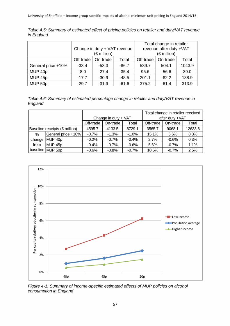
University of Sheffield – Income group-specific impacts of alcohol minimum unit pricing in England 2014/15
57
Table 4.5: Summary of estimated effect of pricing policies on retailer and duty/VAT revenue in England
Change in duty + VAT revenue
(£ million)
Total change in retailer revenue after duty +VAT
(£ million)
Off-trade On-trade Total Off-trade On-trade Total
General price +10% -33.4 -53.3 -86.7 539.7 504.1 1043.9
MUP 40p -8.0 -27.4 -35.4 95.6 -56.6 39.0
MUP 45p -17.7 -30.9 -48.5 201.1 -62.2 138.9
MUP 50p -29.7 -31.9 -61.6 375.2 -61.4 313.9
Table 4.6: Summary of estimated percentage change in retailer and duty/VAT revenue in England
Figure 4-1: Summary of income-specific estimated effects of MUP policies on alcohol consumption in England
Off-trade On-trade Total Off-trade On-trade Total
4595.7 4133.5 8729.1 3565.7 9068.1 12633.8
General price +10% -0.7% -1.3% -1.0% 15.1% 5.6% 8.3%
MUP 40p -0.2% -0.7% -0.4% 2.7% -0.6% 0.3%
MUP 45p -0.4% -0.7% -0.6% 5.6% -0.7% 1.1%
MUP 50p -0.6% -0.8% -0.7% 10.5% -0.7% 2.5%
Change in duty + VAT
Total change in retailer received
after duty +VAT
Baseline receipts (£ million)
%
change
from
baseline
0%
2%
4%
6%
8%
10%
12%
40p 45p 50p
Per
cap
ita
rela
tive
red
uct
ion
in c
on
sum
pti
on
Low income
Population average
Higher income

University of Sheffield – Income group-specific impacts of alcohol minimum unit pricing in England 2014/15
58
Figure 4-2: Summary of income-specific estimated effects of MUP policies on alcohol consumption in England
Figure 4-3: Summary of estimated effects of MUP policies on alcohol consumption in England by income and drinker groups
0%
2%
4%
6%
8%
10%
12%
40p 45p 50p
Per
cap
ita
rela
tive
red
uct
ion
in c
on
sum
pti
on
Harmful
Population average
Hazardous
Moderate
0%
2%
4%
6%
8%
10%
12%
40p 45p 50p
Per
cap
ita
rela
tive
red
uct
ion
in c
on
sum
ptio
n
Low income harmful
Low income hazardous
Higher income harmful
Low income moderate
Higher income moderate
Higher income hazardous

University of Sheffield – Income group-specific impacts of alcohol minimum unit pricing in England 2014/15
59
Table 4.7: Summary of estimated effects of pricing policies on health, crime and workplace related harm in England
Workplace per
annum
Deaths
Illness
('000s)
Hospital
Admissions
('000s)
QALYs
Saved
('000s) Deaths
Illness
('000s)
Hospital
Admissions
('000s)
10 Year
Cumul
Discounted
QALYs
('000s)
Violent
Crimes
('000s)
Criminal
Damage
('000s)
Robbery
Theft Other
('000s)
Total
Crimes
('000s)
Days Absence
('000s)
England population General price +10% -431 -14.8 -19.0 -4.7 -1781 -35.7 -61.1 -77.5 -27.6 -79.3 -14.1 -121.0 -867.3
MUP 40p -74 -2.4 -3.5 -0.8 -379 -7.8 -15.0 -14.8 -4.9 -14.4 -2.5 -21.8 -154.6
MUP 45p -123 -4.0 -5.7 -1.2 -624 -12.5 -23.7 -24.2 -7.8 -22.5 -3.9 -34.2 -247.6
MUP 50p -192 -6.2 -8.7 -1.9 -960 -18.7 -35.1 -37.1 -11.6 -33.2 -5.9 -50.7 -376.6
Low income General price +10% -132 -4.6 -6.3 -1.3 -551 -12.4 -22.6 -24.5
MUP 40p -48 -1.6 -2.3 -0.5 -254 -5.3 -10.3 -9.7
MUP 45p -76 -2.5 -3.6 -0.7 -392 -8.2 -15.6 -15.2
MUP 50p -111 -3.7 -5.2 -1.1 -557 -11.5 -21.8 -21.9
Higher income General price +10% -300 -10.2 -12.8 -3.3 -1,231 -23.2 -38.5 -53.0
MUP 40p -26 -0.8 -1.2 -0.3 -125 -2.5 -4.8 -5.0
MUP 45p -47 -1.5 -2.1 -0.5 -232 -4.3 -8.1 -9.0
MUP 50p -81 -2.6 -3.5 -0.8 -404 -7.2 -13.3 -15.2
Moderate General price +10% -121 -5.3 -6.3 -1.7 -133 -8.1 -11.5 -23.5 -11.4 -32.9 -5.9 -50.3 -353.0
MUP 40p -10 -0.4 -0.5 -0.2 -7 -0.6 -0.8 -2.5 -1.3 -4.0 -0.6 -5.9 -36.3
MUP 45p -17 -0.7 -0.9 -0.2 -11 -1.0 -1.4 -4.1 -1.9 -6.0 -1.0 -8.9 -55.8
MUP 50p -27 -1.2 -1.4 -0.4 -19 -1.7 -2.4 -6.6 -2.9 -8.9 -1.5 -13.3 -87.7
Hazardous General price +10% -161 -5.4 -6.6 -1.8 -695 -11.5 -18.1 -27.1 -10.6 -31.2 -5.4 -47.2 -335.1
MUP 40p -10 -0.4 -0.5 -0.2 -23 -0.5 -0.8 -2.0 -1.3 -4.0 -0.7 -6.1 -42.6
MUP 45p -21 -0.8 -1.0 -0.3 -60 -1.2 -1.8 -3.9 -2.3 -7.0 -1.2 -10.5 -73.9
MUP 50p -39 -1.5 -1.8 -0.5 -129 -2.5 -3.8 -7.1 -3.7 -11.0 -2.0 -16.7 -119.1
Harmful General price +10% -150 -4.1 -6.2 -1.2 -953 -16.0 -31.5 -26.8 -5.5 -15.2 -2.7 -23.5 -179.1
MUP 40p -53 -1.6 -2.4 -0.4 -349 -6.7 -13.4 -10.3 -2.3 -6.4 -1.1 -9.8 -75.8
MUP 45p -85 -2.5 -3.8 -0.7 -554 -10.3 -20.5 -16.2 -3.5 -9.5 -1.7 -14.8 -117.9
MUP 50p -125 -3.6 -5.4 -1.0 -812 -14.5 -29.0 -23.4 -5.0 -13.3 -2.4 -20.7 -169.8
16-17 General price +10% -2 -0.1 -0.2 -0.1 -2 -0.1 -0.2 -0.4 -0.2 -2.6 -0.3 -3.1 -16.1
MUP 40p 0 0.0 0.0 0.0 0 0.0 0.0 -0.1 -0.1 -0.4 0.0 -0.5 -2.7
MUP 45p -1 0.0 -0.1 0.0 0 0.0 -0.1 -0.2 -0.1 -0.7 -0.1 -0.9 -5.3
MUP 50p -1 -0.1 -0.1 0.0 -1 -0.1 -0.1 -0.2 -0.2 -1.1 -0.1 -1.4 -7.9
18-24 Hazardous General price +10% -12 -0.6 -0.8 -0.2 -11 -0.5 -0.7 -1.9 -3.4 -13.1 -1.8 -18.3 -91.4
MUP 40p -2 -0.1 -0.1 0.0 -2 -0.1 -0.1 -0.3 -0.5 -1.7 -0.2 -2.5 -15.5
MUP 45p -3 -0.2 -0.2 -0.1 -3 -0.2 -0.2 -0.5 -0.8 -3.1 -0.4 -4.3 -25.5
MUP 50p -5 -0.2 -0.3 -0.1 -4 -0.2 -0.3 -0.8 -1.3 -4.7 -0.7 -6.6 -38.0
n/a
n/a
n/a
n/a
Population/subgroups Policies
Year 1 Health Harm Full Effect Health Harm in Year 10 per annum Crime per annum
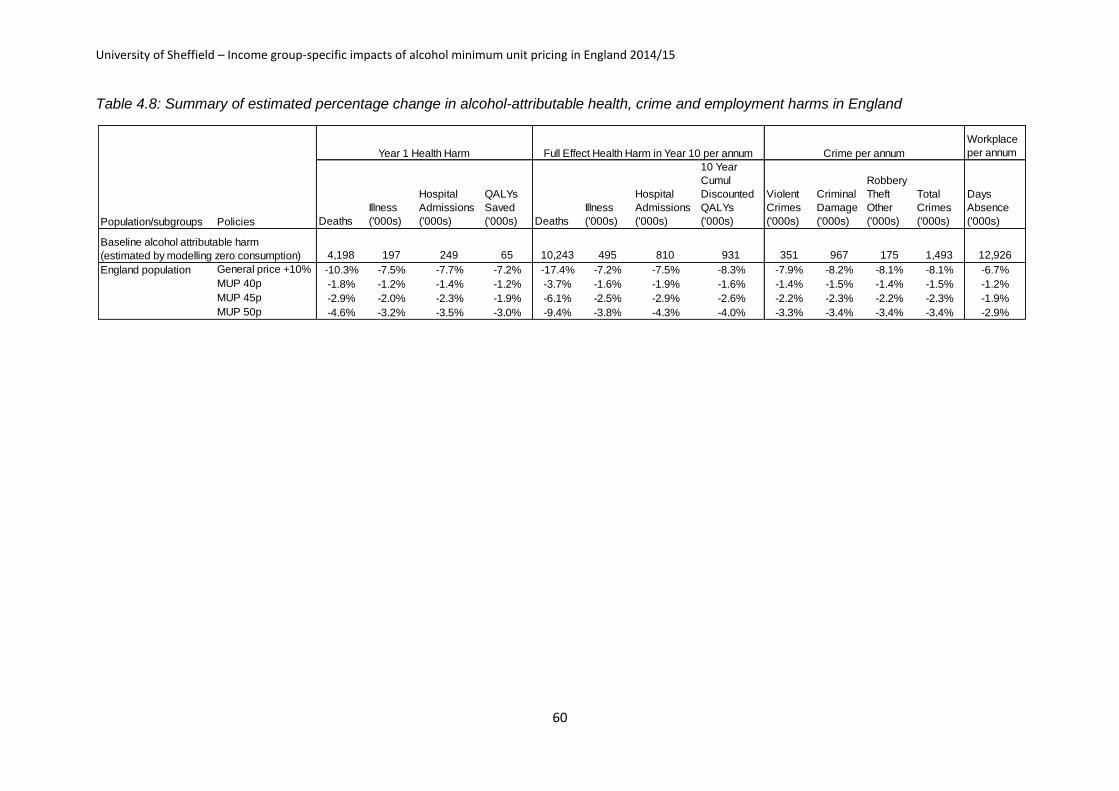
University of Sheffield – Income group-specific impacts of alcohol minimum unit pricing in England 2014/15
60
Table 4.8: Summary of estimated percentage change in alcohol-attributable health, crime and employment harms in England
Workplace
per annum
Deaths
Illness
('000s)
Hospital
Admissions
('000s)
QALYs
Saved
('000s) Deaths
Illness
('000s)
Hospital
Admissions
('000s)
10 Year
Cumul
Discounted
QALYs
('000s)
Violent
Crimes
('000s)
Criminal
Damage
('000s)
Robbery
Theft
Other
('000s)
Total
Crimes
('000s)
Days
Absence
('000s)
4,198 197 249 65 10,243 495 810 931 351 967 175 1,493 12,926
England population General price +10% -10.3% -7.5% -7.7% -7.2% -17.4% -7.2% -7.5% -8.3% -7.9% -8.2% -8.1% -8.1% -6.7%
MUP 40p -1.8% -1.2% -1.4% -1.2% -3.7% -1.6% -1.9% -1.6% -1.4% -1.5% -1.4% -1.5% -1.2%
MUP 45p -2.9% -2.0% -2.3% -1.9% -6.1% -2.5% -2.9% -2.6% -2.2% -2.3% -2.2% -2.3% -1.9%
MUP 50p -4.6% -3.2% -3.5% -3.0% -9.4% -3.8% -4.3% -4.0% -3.3% -3.4% -3.4% -3.4% -2.9%
Population/subgroups Policies
Year 1 Health Harm Full Effect Health Harm in Year 10 per annum Crime per annum
Baseline alcohol attributable harm
(estimated by modelling zero consumption)

University of Sheffield – Income group-specific impacts of alcohol minimum unit pricing in England 2014/15
61
Table 4.9: Summary of financial valuation of impact of pricing policies on health, crime and workplace related harm in England
Healthcare
Costs
Crime
Costs
Absence
Costs
Total
Direct
Costs
Total Value
of Harm
Reduction
incl QALYs
Healthcare
Costs
Crime
Costs
Absence
Costs
Total
Direct
Costs
Total Value of
Harm
Reduction incl
QALYs
England population General price +10% -93.5 -498.1 -97.8 -689.5 -970.8 -1,306.4 -4,142.8 -813.2 -6,262.3 -11,080.6
MUP 40p -15.4 -87.7 -16.7 -119.8 -164.7 -257.5 -729.8 -138.9 -1,126.2 -2,107.6
MUP 45p -25.3 -138.1 -27.0 -190.5 -264.5 -417.2 -1,148.8 -224.8 -1,790.8 -3,381.9
MUP 50p -39.4 -205.9 -41.5 -286.8 -402.5 -634.2 -1,712.6 -345.2 -2,692.1 -5,105.2
Low income General price +10% -28.4 -447.6
MUP 40p -9.8 -173.7
MUP 45p -15.5 -270.4
MUP 50p -22.8 -387.5
Higher income General price +10% -65.1 -858.8
MUP 40p -5.6 -83.8
MUP 45p -9.8 -146.9
MUP 50p -16.6 -246.7
Moderate General price +10% -33.9 -205.7 -40.4 -279.9 -383.2 -364.0 -1,710.5 -336.0 -2,410.5 -3,815.1
MUP 40p -2.9 -22.8 -3.7 -29.5 -38.0 -30.3 -189.8 -30.9 -251.0 -399.2
MUP 45p -4.8 -34.6 -5.9 -45.3 -59.1 -49.5 -287.9 -48.9 -386.3 -627.8
MUP 50p -7.8 -52.5 -9.5 -69.8 -92.7 -82.0 -436.6 -78.9 -597.6 -985.8
Hazardous General price +10% -34.5 -192.0 -37.1 -263.6 -368.9 -443.5 -1,596.9 -308.7 -2,349.1 -3,960.9
MUP 40p -2.8 -23.0 -4.4 -30.2 -38.5 -28.2 -191.1 -36.8 -256.1 -369.9
MUP 45p -5.4 -40.1 -7.8 -53.3 -69.4 -58.4 -333.5 -64.6 -456.5 -683.6
MUP 50p -9.7 -64.0 -12.7 -86.4 -115.3 -110.4 -532.5 -105.5 -748.4 -1,166.1
Harmful General price +10% -25.2 -100.4 -20.3 -145.9 -218.7 -498.8 -835.4 -168.5 -1,502.7 -3,304.6
MUP 40p -9.6 -41.9 -8.6 -60.1 -88.1 -199.0 -348.8 -71.2 -619.0 -1,338.5
MUP 45p -15.1 -63.4 -13.4 -91.9 -136.0 -309.4 -527.4 -111.2 -948.0 -2,070.5
MUP 50p -21.9 -89.4 -19.3 -130.6 -194.5 -441.8 -743.5 -160.8 -1,346.1 -2,953.3
16-17 General price +10% -1.0 -8.3 -0.6 -9.9 -13.2 -8.3 -68.8 -5.2 -82.3 -108.8
MUP 40p -0.2 -1.1 -0.1 -1.4 -2.0 -1.4 -9.5 -0.8 -11.7 -16.7
MUP 45p -0.3 -2.3 -0.2 -2.8 -4.0 -2.7 -18.9 -1.6 -23.2 -32.7
MUP 50p -0.5 -3.5 -0.3 -4.3 -6.0 -4.0 -28.9 -2.4 -35.3 -49.4
18-24 Hazardous General price +10% -3.9 -58.3 -6.3 -68.5 -81.2 -32.3 -484.8 -52.5 -569.6 -685.6
MUP 40p -0.6 -7.7 -1.0 -9.3 -11.6 -5.2 -63.8 -8.7 -77.7 -97.6
MUP 45p -1.1 -13.5 -1.7 -16.3 -19.9 -8.7 -112.5 -14.4 -135.7 -168.3
MUP 50p -1.6 -20.8 -2.6 -25.0 -30.3 -13.1 -172.8 -21.6 -207.5 -256.0
Population/subgroups Policies
Value of Harm Reduction in Year 1 (£millions)
Value of Harm Reduction cumulative over 10 years discounted
(£millions)
n/a n/a
n/a n/a

University of Sheffield – Income group-specific impacts of alcohol minimum unit pricing in England 2014/15
62
Table 4.10: Summary of income-specific estimated effects and financial valuation of impacts of pricing policies on health harm related to alcohol in England
Deaths
Illness
('000s)
Hospital
Admissions
('000s)
QALYs
Saved
('000s) Deaths
Illness
('000s)
Hospital
Admissions
('000s)
10 Year
Cumul
Discounted
QALYs
('000s)
Healthcar
e Costs
Health
QALYs
Value
Total Value
of Health
Harm
Reduction
incl QALYs
Healthcare
Costs
Health
QALYs
Value
Total Value of
Health Harm
Reduction incl
QALYs
Low income moderate General price +10% -34 -1.6 -1.8 -0.5 -29 -2.5 -3.5 -7.1 -10.1 -30.0 -40.0 -112.0 -423.4 -535.4
MUP 40p -6 -0.3 -0.3 -0.1 -3 -0.4 -0.5 -1.6 -1.8 -5.4 -7.2 -18.5 -95.2 -113.7
MUP 45p -9 -0.4 -0.5 -0.1 -4 -0.6 -0.9 -2.5 -2.8 -8.6 -11.4 -30.5 -151.8 -182.3
MUP 50p -14 -0.7 -0.8 -0.2 -7 -1.0 -1.4 -3.8 -4.4 -13.4 -17.8 -48.4 -230.8 -279.3
Low income hazardous General price +10% -38 -1.3 -1.6 -0.4 -162 -2.7 -4.1 -6.4 -8.2 -25.0 -33.1 -105.7 -383.7 -489.4
MUP 40p -10 -0.4 -0.5 -0.1 -40 -0.7 -1.1 -1.9 -2.4 -7.6 -10.0 -29.4 -113.0 -142.4
MUP 45p -16 -0.6 -0.8 -0.2 -68 -1.2 -1.9 -3.1 -3.9 -12.6 -16.5 -49.0 -186.6 -235.6
MUP 50p -26 -1.0 -1.2 -0.3 -108 -1.9 -2.9 -4.8 -6.1 -19.6 -25.7 -76.8 -289.2 -366.0
Low income harmful General price +10% -61 -1.7 -2.9 -0.4 -360 -7.3 -15.0 -11.0 -10.2 -26.0 -36.2 -229.8 -662.2 -892.0
MUP 40p -33 -0.9 -1.5 -0.3 -212 -4.2 -8.6 -6.3 -5.7 -15.3 -20.9 -125.7 -376.7 -502.4
MUP 45p -50 -1.5 -2.3 -0.4 -320 -6.3 -12.9 -9.6 -8.8 -23.7 -32.5 -190.9 -573.7 -764.5
MUP 50p -71 -2.0 -3.2 -0.6 -442 -8.6 -17.4 -13.2 -12.3 -33.4 -45.6 -262.3 -793.4 -1,055.7
Higher income moderateGeneral price +10% -87 -3.7 -4.4 -1.3 -104 -5.6 -8.0 -16.5 -23.8 -75.0 -98.8 -252.0 -988.8 -1,240.8
MUP 40p -4 -0.2 -0.2 -0.1 -4 -0.2 -0.3 -0.9 -1.2 -3.6 -4.8 -11.8 -55.6 -67.4
MUP 45p -7 -0.3 -0.4 -0.1 -7 -0.4 -0.5 -1.6 -2.0 -6.1 -8.0 -19.0 -93.7 -112.7
MUP 50p -13 -0.5 -0.6 -0.2 -12 -0.7 -0.9 -2.7 -3.4 -10.8 -14.2 -33.6 -163.8 -197.5
Higher income hazardousGeneral price +10% -123 -4.1 -5.0 -1.3 -533 -8.9 -14.0 -20.7 -26.3 -80.8 -107.2 -337.8 -1,244.3 -1,582.0
MUP 40p -1 -0.1 -0.1 0.0 17 0.2 0.4 -0.1 -0.5 -1.7 -2.2 1.2 -5.5 -4.3
MUP 45p -4 -0.2 -0.3 -0.1 8 0.0 0.0 -0.8 -1.5 -5.0 -6.5 -9.3 -46.8 -56.2
MUP 50p -13 -0.5 -0.7 -0.2 -21 -0.6 -0.8 -2.3 -3.6 -11.4 -15.0 -33.6 -137.3 -170.9
Higher income harmful General price +10% -89 -2.4 -3.3 -0.7 -593 -8.7 -16.5 -15.8 -15.0 -44.0 -59.0 -269.0 -945.5 -1,214.5
MUP 40p -21 -0.6 -0.9 -0.2 -138 -2.4 -4.8 -4.0 -4.0 -11.7 -15.6 -73.3 -241.6 -314.9
MUP 45p -35 -1.0 -1.5 -0.3 -234 -3.9 -7.7 -6.6 -6.4 -18.7 -25.1 -118.5 -396.5 -515.0
MUP 50p -55 -1.5 -2.2 -0.5 -370 -5.9 -11.5 -10.2 -9.6 -28.3 -37.9 -179.5 -610.0 -789.5
Value of Harm Reduction in Year
1 (£millions)
Value of Harm Reduction cumulative
discounted (£millions)Year 1 Health Harm Full Effect Health Harm in Year 10 per annum
Population/subgroups Policies

University of Sheffield – Income group-specific impacts of alcohol minimum unit pricing in England 2014/15
63
4.2 EXAMPLE POLICY ANALYSIS: 45P MUP (2014/15 PRICES)
The estimated impacts of a 45p MUP policy in 2014/15 prices are described in detail in this
section. We assume that the threshold is updated annually in line with inflation.
In addition to the results shown in Tables 4.1 to 4.10, Tables 4.11 to 4.14 show further
detailed results for consumption changes, consumer spending and sales for a 45p MUP
policy. Table 4.15 shows the estimated relative change in price for the 10 modelled
beverage types and beverage-specific changes in consumption and spending for a 45p MUP
policy. Detailed results for other modelled policies are not presented here but are available
from the authors.
Across the whole population, 23.2% of alcohol units purchased would be affected.
The proportion and absolute number of purchased units per week affected for harmful
drinkers (30.5% or 21.8 units) is substantially greater than for hazardous (19.5% or 5.3 units)
or moderate drinkers (12.5% or 0.7 units). The proportion and number of purchased units
per week affected is also greater for low income vs. higher income drinkers in each of the
moderate (18.4% vs. 10.5% or 0.8 vs. 0.6 units), hazardous (29.0% vs. 16.8% or 7.9 vs. 4.6
units) and harmful (40.7% vs. 28.0% or 31.0 vs. 19.6 units) drinker groups.
Across the whole population, weekly consumption changes by -1.6% on average.
Consumption is estimated to reduce by 0.19 units per person or 0.23 units per drinker per
week. Weekly consumption reductions are larger for harmful drinkers (-3.7% or -2.62 units)
than moderate drinkers (-0.6% or -0.03 units) and for those with low incomes (-4.3% or -0.54
units) compared to those with higher incomes (-0.9% or -0.13 units).
In both the low and higher income groups, consumption reductions are small for
moderate drinkers and larger for harmful drinkers. Estimated consumption reductions for
low income moderate drinkers are -1.5% or -0.07 units compared to -7.5% or -5.70 units for
low income harmful drinkers. The corresponding figures for higher income moderate and
harmful drinkers are -0.3% or -0.02 units and -2.3% or -1.63 units.
The small impact on moderate drinkers reflects the small amount of alcohol purchased for
less than 45p per unit by moderate drinkers in either income group. In contrast, the larger
impacts on harmful drinkers, and particularly harmful drinkers with low incomes, reflects the
larger quantities of alcohol purchased below the MUP threshold by these groups.
Across the whole population, spending increases by 0.4% or £2.60 per drinker per
year. The cost impact of the policy on consumer spending also varies substantially between
drinker and income subgroups. Annual spending increases are larger for hazardous drinkers

University of Sheffield – Income group-specific impacts of alcohol minimum unit pricing in England 2014/15
64
(£9.70) than moderate drinkers (£0.90) and it is estimated that spending slightly decreases
for harmful drinkers (-£1.70). Unlike the consumption results, the impacts on annual
spending are estimated to be greater for higher income drinkers (£3.90), while low income
drinkers are estimated to slightly decrease their spending (-£1.70). For higher income groups,
increases in spending are larger for harmful drinkers (£9.70) than moderate drinkers (£1.10).
However, for low income groups, we see a significant reduction in estimated spending
changes for harmful drinkers (-£37.40), mainly driven by reductions in spending on off-trade
cider, and a small increase for moderate drinkers (£0.30). Within each drinker category,
higher income drinkers see larger increases in their annual alcohol spending than low
income drinkers. This difference is a result of the different price elasticities of the beverages
which greater or lesser proportions of each subgroup’s alcohol purchases.
Overall revenue to the Treasury (from duty and VAT receipts) changes by -£48.5m
(-17.7m and -£30.9m for off- and on-trade).
Revenue to off- retailers is estimated to increase by £201.1m in the off-trade and
decrease by £62.2m in the on-trade.
As with previous results from SAPM, the estimated impacts on revenue to the Treasury are
broadly neutral as falling duty receipts due to lower sales are largely matched by increased
VAT receipts due to the higher value of the remaining sales.
Effects on health are estimated to be substantial with alcohol-attributable deaths
estimated to reduce by approximately 123 per annum in the first year following
implementation and by 624 per annum from the tenth year, by which time the model
assumes the full effects of the policy will be seen. Annual reductions in deaths from year 10
are distributed differentially across the drinker groups, with approximately 11 saved amongst
moderate drinkers, 60 amongst hazardous drinkers and 554 amongst harmful drinkers.
Larger reductions in deaths per annum from year 10 are also seen amongst low income
drinkers (-392) than higher income drinkers (-232).
Alcohol-attributable morbidity also decreases with an estimated reduction of 12,500 illnesses
and 23,700 hospital admission per annum across all drinkers from year 10. Direct healthcare
service costs are estimated to reduce by £25.3m in year 1 and by £417.2m in total over the
first ten years of the policy.
Crime is estimated to fall by 34,200 offences per year overall. Almost 43% of this annual
reduction, or 14,800 crimes, are attributable to harmful drinkers who account for around 5%
of the population. A further 31% or 10,500 fewer crimes are attributable to hazardous

University of Sheffield – Income group-specific impacts of alcohol minimum unit pricing in England 2014/15
65
drinkers who account for around 18% of the population. Costs of crime are estimated to
reduce by £138.1m per year.
Workplace absence is estimated to be reduced by 247,600 days per year. This is
estimated to lead to savings of £27m per year.
The total societal value of these harm reductions to health, crime and workplace
absence is estimated at £3.4bn in total over the 10 year period modelled. This includes
both direct costs and gains in QALYs. In the first year, the estimated societal value of the
harm reductions is as follows: NHS direct cost reductions (£25.3m), crime costs saved
(£138.1m), workplace absences avoided (£27.0m), and the total year 1 value of harm
reduction including health QALYs is £264.5m. The societal value of the £3.4bn of harm
reductions over the 10 year period is distributed differentially across the drinker groups, with
reductions in alcohol consumption among harmful drinkers accounting for 61.2% of the total
value, hazardous drinkers 20.2% and moderate drinkers 18.6%.

University of Sheffield – Income group-specific impacts of alcohol minimum unit pricing in England 2014/15
66
Table 4.11: Detailed results for 45p MUP (consumption and spending effects)
Population Moderate Hazardous Harmful Low income
Higher
income 16-17
18-24
Hazardous
Baseline statistics
Baseline Consumption (units per week) 11.9 4.3 27.2 71.4 9.3 12.9 7.8 27.6
Population 41,393,296 31,964,234 7,232,457 2,196,605 11,224,815 30,168,481 1,041,951 655,712
Baseline Consumption (drinker) 14.1 5.5 27.2 71.4 12.7 14.6 11.0 27.6
Drinker population 34,889,490 25,460,428 7,232,457 2,196,605 8,213,926 26,675,564 738,841 655,712
% drinkers 84.3% 79.7% 100.0% 100.0% 73.2% 88.4% 70.9% 100.0%
% binge (>8 male, >6 female) 21.7% 11.4% 49.4% 79.4% 14.8% 24.2% 16.3% 70.8%
Mean binge if binge occurs 12.1 10.2 12.4 15.1 12.7 12.0 12.5 14.6
Sales/Consumption volume, units per drinker per year
Off-beer 96.8 29.6 169.6 636.0 113.5 91.6 40.0 128.1
Off-cider 18.9 4.8 24.8 162.6 33.4 14.4 24.9 17.1
Off-wine 264.5 92.1 584.2 1,210.0 175.1 292.0 86.1 184.6
Off-spirits 71.1 27.2 128.1 392.3 93.3 64.3 23.6 157.9
Off-RTDs 7.8 2.1 8.7 71.7 10.1 7.2 16.4 18.7
On-beer 199.4 80.2 371.4 1,014.7 187.7 203.0 163.2 555.0
On-cider 7.7 3.2 13.2 42.5 6.6 8.1 11.0 34.7
On-wine 37.9 26.8 68.0 68.3 15.5 44.8 27.0 57.8
On-spirits 19.8 14.2 31.6 46.0 14.9 21.3 62.8 160.3
On-RTDs 12.3 4.5 19.6 78.0 11.5 12.5 118.9 124.7
Total 736.2 284.5 1,419.3 3,722.1 661.6 759.1 573.9 1,438.9
Spending, per drinker per year (£)
Off-beer 43.08 14.54 76.51 263.83 48.64 41.37 12.33 56.01
Off-cider 7.03 2.14 9.81 54.58 11.23 5.74 10.88 7.11
Off-wine 143.16 51.74 314.08 639.95 83.73 161.46 4.49 97.34
Off-spirits 34.60 14.23 61.86 180.91 42.90 32.04 2.50 74.69
Off-RTDs 6.05 1.99 7.07 49.67 7.46 5.61 2.36 19.92
On-beer 246.57 104.80 455.97 1,200.37 212.72 257.00 179.67 698.52
On-cider 9.27 3.98 15.98 48.53 6.80 10.04 5.60 41.23
On-wine 52.04 37.19 91.73 93.57 17.93 62.54 24.06 77.08
On-spirits 48.34 36.23 74.68 102.05 33.04 53.05 128.78 368.00
On-RTDs 22.15 8.58 34.87 137.60 18.93 23.14 188.48 226.85
Total 612.30 275.43 1,142.56 2,771.06 483.38 652.00 559.15 1,666.74
After intervention / Change from baseline
Changes in consumption (units per week) -0.19 -0.02 -0.18 -2.62 -0.40 -0.11 -0.03 -0.41
Changes in consumption (drinker) -0.23 -0.03 -0.18 -2.62 -0.54 -0.13 -0.05 -0.41
Changes in consumption (%) -1.6% -0.6% -0.7% -3.7% -4.3% -0.9% -0.4% -1.5%
Final Consumption (drinker) 13.9 5.4 27.0 68.8 12.1 14.4 11.0 27.2
Absolute change in sales/Consumption volume, units per drinker per year
Off-beer -5.7 -0.8 -8.8 -52.9 -7.2 -5.3 -1.9 -7.8
Off-cider -7.2 -1.0 -8.2 -75.8 -16.4 -4.3 -0.6 -3.6
Off-wine 8.0 1.6 18.1 49.3 5.3 8.8 0.2 4.4
Off-spirits -3.7 -0.8 -6.6 -27.8 -5.2 -3.2 -0.6 -6.0
Off-RTDs -1.1 -0.1 -1.2 -12.0 -1.7 -0.9 -0.3 -2.3
On-beer -3.1 -0.9 -5.0 -22.1 -3.7 -2.9 -0.5 -5.8
On-cider 0.2 0.1 0.3 1.4 0.2 0.2 0.0 0.7
On-wine 1.1 0.6 2.3 3.3 0.5 1.3 0.2 1.8
On-spirits -0.4 -0.2 -0.6 -1.5 -0.4 -0.4 0.0 -3.4
On-RTDs 0.1 0.0 0.2 1.6 0.3 0.1 1.1 0.7
Total -11.7 -1.6 -9.5 -136.6 -28.2 -6.7 -2.5 -21.4
Absolute change in spending, per drinker per year (£)
Off-beer 0.59 0.16 1.09 3.85 0.88 0.49 -0.05 0.52
Off-cider -1.36 -0.16 -1.55 -14.67 -3.22 -0.79 0.82 -0.55
Off-wine 7.72 2.01 16.22 45.99 6.37 8.14 0.09 5.44
Off-spirits -0.74 -0.07 -1.46 -6.20 -0.72 -0.75 0.02 -0.10
Off-RTDs -0.95 -0.14 -0.94 -10.32 -1.37 -0.82 -0.04 -2.48
On-beer -3.71 -1.14 -5.95 -26.12 -4.15 -3.57 -0.49 -7.19
On-cider 0.24 0.08 0.42 1.63 0.26 0.24 0.00 0.82
On-wine 1.51 0.78 3.09 4.69 0.65 1.77 0.20 2.42
On-spirits -0.97 -0.61 -1.48 -3.47 -0.91 -0.98 -0.08 -7.91
On-RTDs 0.25 0.01 0.29 2.91 0.48 0.19 1.74 1.19
Total 2.59 0.93 9.75 -1.70 -1.74 3.92 2.23 -7.83
Relative change in spending 0.4% 0.3% 0.9% -0.1% -0.4% 0.6% 0.4% -0.5%

University of Sheffield – Income group-specific impacts of alcohol minimum unit pricing in England 2014/15
67
Table 4.12: Detailed income and drinker group-specific results for 45p MUP (consumption and spending effects)
Low income
moderate
Low income
hazardous
Low income
harmful
Higher income
moderate
Higher income
hazardous
Higher income
harmful
Baseline statistics
Baseline Consumption (units per week) 3.1 27.2 76.2 4.9 27.2 69.8
Population 9,418,385 1,273,410 533,020 22,545,849 5,959,047 1,663,585
Baseline Consumption (drinker) 4.5 27.2 76.2 5.8 27.2 69.8
Drinker population 6,407,497 1,273,410 533,020 19,052,931 5,959,047 1,663,585
% drinkers 68.0% 100.0% 100.0% 84.5% 100.0% 100.0%
% binge (>8 male, >6 female) 7.0% 47.3% 74.9% 13.3% 49.8% 80.8%
Mean binge if binge occurs 9.9 13.2 16.0 10.3 12.2 14.8
Sales/Consumption volume, units per drinker per year
Off-beer 31.7 233.9 808.8 28.8 155.9 580.7
Off-cider 5.2 48.2 337.0 4.6 19.8 106.8
Off-wine 70.4 442.7 794.7 99.3 614.4 1,343.1
Off-spirits 33.5 186.2 591.0 25.1 115.7 328.6
Off-RTDs 2.7 18.0 80.4 1.9 6.7 68.9
On-beer 64.0 390.5 1,190.2 85.6 367.3 958.5
On-cider 1.9 17.6 36.6 3.6 12.3 44.4
On-wine 10.8 31.8 32.9 32.1 75.8 79.6
On-spirits 11.0 22.4 44.0 15.3 33.6 46.6
On-RTDs 4.4 27.3 58.8 4.6 18.0 84.1
Total 235.6 1,418.6 3,974.5 300.9 1,419.5 3,641.3
Spending, per drinker per year (£)
Off-beer 4.80 100.76 328.55 14.39 71.33 243.09
Off-cider 0.73 16.70 106.36 2.11 8.34 37.99
Off-wine 11.90 209.88 372.04 57.48 336.35 725.79
Off-spirits 5.73 83.07 258.10 13.30 57.33 156.18
Off-RTDs 0.82 13.36 53.83 1.84 5.73 48.34
On-beer 23.81 446.46 1,288.72 114.23 458.00 1,172.06
On-cider 0.72 19.09 31.80 4.56 15.32 53.89
On-wine 4.32 36.25 35.77 45.38 103.58 112.09
On-spirits 8.58 46.59 91.50 39.84 80.68 105.43
On-RTDs 2.72 46.14 86.31 8.80 32.47 154.03
Total 64.14 1,018.29 2,652.99 301.94 1,169.12 2,808.89
After intervention / Change from baseline
Changes in consumption (units per week) -0.05 -0.77 -5.70 -0.02 -0.06 -1.63
Changes in consumption (drinker) -0.07 -0.77 -5.70 -0.02 -0.06 -1.63
Changes in consumption (%) -1.5% -2.8% -7.5% -0.3% -0.2% -2.3%
Final Consumption (drinker) 4.5 26.4 70.5 5.8 27.2 68.2
Absolute change in sales/Consumption volume, units per drinker per year
Off-beer -1.1 -14.0 -64.4 -0.7 -7.7 -49.2
Off-cider -1.3 -21.5 -185.8 -0.9 -5.4 -40.6
Off-wine 0.9 15.4 34.4 1.8 18.7 54.1
Off-spirits -0.9 -10.7 -43.3 -0.7 -5.7 -22.8
Off-RTDs -0.2 -2.9 -16.2 -0.1 -0.8 -10.6
On-beer -0.9 -8.0 -26.2 -0.9 -4.3 -20.8
On-cider 0.1 0.7 1.4 0.1 0.3 1.4
On-wine 0.3 1.3 1.9 0.7 2.5 3.7
On-spirits -0.3 -0.7 -1.7 -0.2 -0.6 -1.5
On-RTDs 0.0 0.4 2.9 0.0 0.1 1.2
Total -3.5 -40.0 -297.0 -1.0 -2.9 -85.2
Absolute change in spending, per drinker per year (£)
Off-beer 0.20 2.00 6.41 0.15 0.90 3.03
Off-cider -0.21 -4.22 -37.04 -0.14 -0.98 -7.50
Off-wine 1.82 16.12 37.84 2.07 16.24 48.61
Off-spirits -0.04 -1.31 -7.59 -0.08 -1.49 -5.76
Off-RTDs -0.22 -2.20 -13.13 -0.11 -0.68 -9.42
On-beer -1.12 -9.12 -28.73 -1.14 -5.27 -25.28
On-cider 0.06 0.76 1.44 0.08 0.35 1.70
On-wine 0.34 1.60 2.12 0.93 3.41 5.52
On-spirits -0.58 -1.34 -3.88 -0.62 -1.50 -3.34
On-RTDs 0.04 0.74 5.14 0.01 0.20 2.19
Total 0.28 3.03 -37.42 1.15 11.18 9.75
Relative change in spending 0.4% 0.3% -1.4% 0.4% 1.0% 0.3%

University of Sheffield – Income group-specific impacts of alcohol minimum unit pricing in England 2014/15
68
Table 4.13: Detailed male income and drinker group specific results for 45p MUP (consumption and spending effects)
Low
income
male
moderate
Low
income
male
hazardous
Low
income
male
harmful
Higher
income
male
moderate
Higher
income
male
hazardous
Higher
income
male
harmful
Baseline statistics
Baseline Consumption (units per week) 4.6 32.3 88.0 6.5 31.5 77.8
Population 3,729,369 665,358 329,900 10,310,984 3,331,242 993,115
Baseline Consumption (drinker) 6.3 32.3 88.0 7.5 31.5 77.8
Drinker population 2,719,609 665,358 329,900 8,975,155 3,331,242 993,115
% drinkers 72.9% 100.0% 100.0% 87.0% 100.0% 100.0%
% binge (>8 male, >6 female) 9.4% 43.8% 77.1% 15.0% 49.4% 81.4%
Mean binge if binge occurs 11.0 13.9 17.3 12.1 13.7 16.7
Sales/Consumption volume, units per drinker per year
Off-beer 54.4 299.4 1,058.4 45.1 218.9 754.0
Off-cider 7.9 57.6 429.9 6.3 25.7 130.9
Off-wine 58.9 354.7 556.1 88.2 509.7 1,008.7
Off-spirits 38.3 179.5 558.6 25.6 113.3 373.3
Off-RTDs 2.7 7.9 22.2 0.9 3.9 15.5
On-beer 133.9 677.0 1,800.0 164.3 620.3 1,522.3
On-cider 3.4 27.5 48.0 6.4 19.2 66.8
On-wine 11.5 37.2 29.1 37.2 87.2 71.6
On-spirits 12.4 24.4 38.2 14.9 32.1 51.7
On-RTDs 3.7 17.1 50.2 2.7 11.7 64.1
Total 327.1 1,682.2 4,590.7 391.7 1,642.0 4,059.0
Spending, per drinker per year (£)
Off-beer 7.84 130.74 431.25 22.46 100.50 316.34
Off-cider 0.97 19.00 124.95 2.89 10.72 46.08
Off-wine 8.97 174.77 273.98 52.05 288.60 589.11
Off-spirits 5.65 80.76 247.59 13.44 55.90 179.11
Off-RTDs 0.76 8.56 0.04 0.85 2.46 14.47
On-beer 48.49 771.74 1,968.24 218.47 773.04 1,858.17
On-cider 1.23 29.67 39.85 8.16 23.96 80.71
On-wine 4.20 42.73 33.63 53.84 120.05 106.83
On-spirits 8.45 48.44 75.02 37.87 75.69 118.83
On-RTDs 1.98 31.06 69.13 5.25 22.06 117.40
Total 88.53 1,337.47 3,263.68 415.28 1,472.98 3,427.07
After intervention / Change from baseline
Changes in consumption (units per week) -0.09 -1.02 -7.53 -0.04 -0.19 -2.47
Changes in consumption (drinker) -0.12 -1.02 -7.53 -0.05 -0.19 -2.47
Changes in consumption (%) -1.9% -3.2% -8.5% -0.6% -0.6% -3.2%
Final Consumption (drinker) 6.2 31.2 80.5 7.5 31.3 75.4
Absolute change in sales/Consumption volume, units per drinker per year
Off-beer -1.7 -14.2 -79.8 -1.1 -10.3 -62.1
Off-cider -2.3 -29.9 -262.6 -1.2 -7.3 -50.4
Off-wine 1.0 15.8 28.0 1.7 18.3 42.9
Off-spirits -1.1 -11.2 -42.4 -0.8 -6.1 -25.9
Off-RTDs -0.3 -1.3 -0.8 -0.1 -0.5 -3.0
On-beer -1.9 -14.2 -39.4 -1.7 -7.3 -33.6
On-cider 0.1 1.1 1.8 0.1 0.4 2.1
On-wine 0.3 1.6 1.7 0.8 3.0 3.4
On-spirits -0.4 -0.9 -1.5 -0.3 -0.5 -2.2
On-RTDs -0.1 0.1 2.6 0.0 0.3 0.4
Total -6.3 -53.1 -392.5 -2.5 -10.1 -128.6
Absolute change in spending, per drinker per year (£)
Off-beer 0.38 3.14 8.97 0.22 1.32 4.14
Off-cider -0.40 -6.13 -54.81 -0.20 -1.37 -9.32
Off-wine 1.42 13.50 25.94 1.83 14.82 38.38
Off-spirits -0.13 -2.16 -10.04 -0.16 -1.73 -7.20
Off-RTDs -0.26 -1.40 -0.01 -0.06 -0.25 -2.78
On-beer -2.35 -16.05 -43.64 -2.23 -8.90 -40.80
On-cider 0.12 1.22 1.87 0.15 0.54 2.53
On-wine 0.38 1.89 2.02 1.21 4.09 5.20
On-spirits -0.82 -1.70 -3.69 -0.75 -1.20 -4.91
On-RTDs -0.08 0.34 5.11 -0.04 0.48 0.64
Total -1.75 -7.35 -68.28 -0.04 7.79 -14.13
Relative change in spending -2.0% -0.5% -2.1% 0.0% 0.5% -0.4%
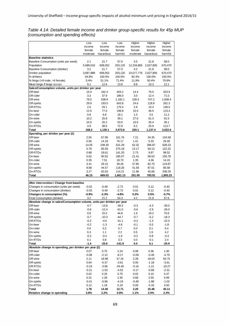
University of Sheffield – Income group-specific impacts of alcohol minimum unit pricing in England 2014/15
69
Table 4.14: Detailed female income and drinker group-specific results for 45p MUP (consumption and spending effects)
Low
income
female
moderate
Low
income
female
hazardous
Low
income
female
harmful
Higher
income
female
moderate
Higher
income
female
hazardous
Higher
income
female
harmful
Baseline statistics
Baseline Consumption (units per week) 2.1 21.7 57.0 3.5 21.8 58.0
Population 5,689,016 608,052 203,120 12,234,865 2,627,805 670,470
Baseline Consumption (drinker) 3.2 21.7 57.0 4.2 21.8 58.0
Drinker population 3,687,888 608,052 203,120 10,077,776 2,627,805 670,470
% drinkers 64.8% 100.0% 100.0% 82.4% 100.0% 100.0%
% binge (>8 male, >6 female) 5.4% 51.1% 71.4% 11.9% 50.4% 79.9%
Mean binge if binge occurs 9.1 12.6 13.8 8.8 10.3 12.1
Sales/Consumption volume, units per drinker per year
Off-beer 15.0 162.3 403.2 14.4 76.0 323.9
Off-cider 3.3 37.9 186.0 3.0 12.4 71.0
Off-wine 79.0 538.9 1,182.1 109.3 747.2 1,838.4
Off-spirits 29.9 193.5 643.8 24.6 118.8 262.3
Off-RTDs 2.6 29.1 175.0 2.8 10.4 148.0
On-beer 12.5 77.0 199.8 15.5 46.5 123.4
On-cider 0.8 6.8 18.1 1.0 3.5 11.2
On-wine 10.2 25.8 39.1 27.6 61.3 91.5
On-spirits 10.0 20.2 53.5 15.6 35.4 39.1
On-RTDs 4.9 38.6 72.9 6.2 25.9 113.7
Total 168.2 1,130.1 2,973.6 220.1 1,137.4 3,022.6
Spending, per drinker per year (£)
Off-beer 2.55 67.96 161.76 7.21 34.35 134.58
Off-cider 0.56 14.18 76.17 1.41 5.33 26.00
Off-wine 14.05 248.30 531.29 62.32 396.87 928.23
Off-spirits 5.78 85.59 275.18 13.17 59.13 122.22
Off-RTDs 0.88 18.61 141.20 2.73 9.87 98.52
On-beer 5.62 90.52 185.07 21.41 58.63 155.78
On-cider 0.35 7.51 18.73 1.35 4.36 14.15
On-wine 4.41 29.15 39.26 37.85 82.70 119.87
On-spirits 8.68 44.57 118.26 41.59 87.01 85.58
On-RTDs 3.27 62.63 114.21 11.96 45.66 208.29
Total 46.15 669.03 1,661.13 201.00 783.91 1,893.23
After intervention / Change from baseline
Changes in consumption (units per week) -0.02 -0.49 -2.72 0.01 0.12 -0.40
Changes in consumption (drinker) -0.03 -0.49 -2.72 0.01 0.12 -0.40
Changes in consumption (%) -0.9% -2.3% -4.8% 0.2% 0.5% -0.7%
Final Consumption (drinker) 3.2 21.2 54.3 4.2 21.9 57.6
Absolute change in sales/Consumption volume, units per drinker per year
Off-beer -0.7 -13.8 -39.3 -0.3 -4.3 -30.0
Off-cider -0.6 -12.4 -61.0 -0.6 -2.9 -26.0
Off-wine 0.8 15.0 44.8 1.9 19.2 70.6
Off-spirits -0.7 -10.3 -44.7 -0.7 -5.2 -18.3
Off-RTDs -0.2 -4.6 -41.1 -0.2 -1.3 -22.0
On-beer -0.2 -1.3 -4.8 -0.1 -0.5 -1.8
On-cider 0.0 0.2 0.7 0.0 0.1 0.4
On-wine 0.3 1.1 2.2 0.5 1.9 4.2
On-spirits -0.2 -0.4 -1.9 -0.2 -0.8 -0.4
On-RTDs 0.1 0.8 3.3 0.0 -0.1 2.4
Total -1.4 -25.6 -141.9 0.4 6.1 -20.9
Absolute change in spending, per drinker per year (£)
Off-beer 0.07 0.75 2.24 0.08 0.36 1.40
Off-cider -0.08 -2.12 -8.17 -0.09 -0.49 -4.79
Off-wine 2.11 18.98 57.16 2.28 18.04 63.75
Off-spirits 0.04 -0.37 -3.61 0.00 -1.18 -3.61
Off-RTDs -0.19 -3.06 -34.45 -0.16 -1.21 -19.27
On-beer -0.21 -1.53 -4.52 -0.17 -0.66 -2.31
On-cider 0.02 0.25 0.75 0.02 0.10 0.47
On-wine 0.31 1.28 2.30 0.68 2.55 5.99
On-spirits -0.41 -0.96 -4.19 -0.49 -1.88 -1.02
On-RTDs 0.12 1.18 5.19 0.05 -0.16 4.50
Total 1.78 14.40 12.71 2.20 15.48 45.11
Relative change in spending 3.8% 2.2% 0.8% 1.1% 2.0% 2.4%

University of Sheffield – Income group-specific impacts of alcohol minimum unit pricing in England 2014/15
70
4.15: Relative change in price for the modelled beverage types and beverage-specific impacts for 45p MUP on consumption and spending
% change in price
Change in consumption
Change in spending
Off-trade beer 8.1% -5.9% 1.4%
Off-trade cider 27.4% -38.1% -19.4%
Off-trade wine 2.4% 3.0% 5.4%
Off-trade spirits 3.3% -5.2% -2.1%
Off-trade RTDs 0.1% -14.1% -15.6%
Subtotal: Off-trade 4.6% -2.1% 2.2%
On-trade beer 0.0% -1.5% -1.5%
On-trade cider 0.0% 2.6% 2.6%
On-trade wine 0.0% 2.9% 2.9%
On-trade spirits 0.0% -2.0% -2.0%
On-trade RTDs 0.0% 1.2% 1.2%
Subtotal: On-trade 0.0% -0.7% -0.7%
Subtotal: beer -3.0% -1.1%
Subtotal: cider -26.3% -6.8%
Subtotal: wine 3.0% 4.7%
Subtotal: spirits -4.5% -2.1%
Subtotal: RTDs -4.8% -2.5%
Total 2.0% -1.6% 0.4%
4.3 SENSITIVITY ANALYSES
A probabilistic sensitivity analysis (PSA) to reflect uncertainty in the estimated elasticities
used for the base case econometric model has been generated for a 45p MUP using 30
samples from the underlying variance-covariance matrices (derived from the econometric
model). Estimated 95% confidence intervals for the change in mean consumption for the
English population and selected subgroups are shown in Table 4.16.
Table 4.16: Probabilistic sensitivity analysis confidence interval estimates
Drink type Central estimate Lower 95% CI Upper 95% CI
All -1.6% -0.3% -3.2%
Low income -4.3% -2.5% -6.4%
Higher income -0.9% 0.4% -2.4%
Moderate -0.6% 0.2% -1.4%
Hazardous -0.7% 0.8% -2.3%
Harmful -3.7% -1.9% -6.2%

University of Sheffield – Income group-specific impacts of alcohol minimum unit pricing in England 2014/15
71
This uncertainty analysis has also examined the relative impact on low versus higher income
groups and moderate versus harmful drinkers. Scatter plots are shown in Figures 4.4 and
4.5. Each point shown is an individual PSA result. A line of equal effect is plotted for each
figure: estimates below and to the right of the line indicate that the low income group (or
harmful drinkers) are affected more in relative terms by the policy than higher income group
(or moderate drinkers). As is apparent from the plots, both low income group and harmful
drinkers are estimated with a high degree of confidence to be more affected by a 45p MUP
than higher income group or moderate drinkers respectively.
Figure 4-4: Scatter plot of PSA results, showing relative change in consumption for a 45p MUP by low income and higher income groups
-10%
-8%
-6%
-4%
-2%
0%
2%
-10% -5% 0%
Ch
ange
in lo
w in
com
e m
ean
co
nsu
mp
tio
n
Change in higher income mean consumption
45p MUP Line of equal effect
Low income drinkers more affected
Higher income drinkers more affected

University of Sheffield – Income group-specific impacts of alcohol minimum unit pricing in England 2014/15
72
Figure 4-5: Scatter plot of PSA results, showing relative change in consumption for a 45p MUP by moderate and harmful drinkers
Table 4.17 and Figures 4.6 and 4.7 compare the estimated impacts on alcohol consumption
of a 45p MUP and a general 10% price increase policy using alternative elasticities as
described in Section 3.8.
-10%
-8%
-6%
-4%
-2%
0%
2%
-10% -5% 0%C
han
ge in
har
mfu
l me
an c
on
sum
pti
on
Change in moderate mean consumption
45p MUP Line of equal effect
Moderate drinkers more affected
Harmful drinkers more affected

University of Sheffield – Income group-specific impacts of alcohol minimum unit pricing in England 2014/15
73
Table 4.17: Comparison of estimated impacts on alcohol consumption for a 45p MUP and a general 10% increase policy using alternative elasticities
45p MUP: Alternative elasticities
Base case
SA1: No cross-
price
SA2: No non-
significant
SA3: Income-specific
SA4: Consumption level-specific
SA5: Time series
SA6: HMRC
Population -1.6% -2.4% -2.3% -1.7% -3.1% -1.9% -2.8%
Low income -4.3% -4.5% -4.4% -8.6% -5.3% -2.9% -5.1%
Higher income -0.9% -1.8% -1.7% 0.1% -2.5% -1.6% -2.1%
Moderate -0.6% -1.0% -1.0% -0.7% -0.4% -0.5% -1.3%
Hazardous -0.7% -1.7% -1.7% -0.5% -2.8% -1.6% -2.1%
Harmful -3.7% -4.3% -4.2% -4.2% -5.8% -3.4% -4.9%
10% price increase: Alternative elasticities
Base case
SA1: No cross-
price
SA2: No non-
significant
SA3: Income-specific
SA4: Consumption level-specific
SA5: Time series
SA6: HMRC
Population -5.0% -6.0% -4.8% -5.0% -5.1% -7.4% -4.3%
Low income -6.0% -6.2% -5.1% -4.8% -6.5% -7.1% -5.1%
Higher income -4.7% -5.9% -4.7% -5.0% -4.7% -7.5% -4.1%
Moderate -4.4% -6.1% -4.4% -4.5% -3.4% -7.9% -4.3%
Hazardous -4.7% -5.8% -4.8% -4.7% -5.1% -7.5% -4.0%
Harmful -5.8% -6.1% -5.2% -5.7% -6.6% -6.9% -4.7%
Remarks: SA1: assuming all cross-price elasticities to be zero (i.e. assuming no substitution effects)
in the elasticity matrix estimated for the base case. SA2: excluding non-significant elasticities (p-value
greater than 0.05) in the elasticity matrix estimated for the base case, SA3: separate low income and
higher income specific-elasticity matrices were estimated using the pseudo-panel approach, SA4:
separate moderate and hazardous/harmful-specific elasticity matrices were estimated using the
pseudo-panel approach, SA5: elasticities were estimated using a time series analysis [30] of national
aggregate data on alcohol released for consumption or sale in the UK from 1964 to 2011. SA6: latest
elasticities estimated by HMRC in 2012.

University of Sheffield – Income group-specific impacts of alcohol minimum unit pricing in England 2014/15
74
Figure 4-6: Comparison of estimated impacts on alcohol consumption of a 45p MUP policy using alternative elasticities.
Figure 4-7: Comparison of estimated impacts on alcohol consumption of a 10% price increase policy using alternative elasticities
-2%
0%
2%
4%
6%
8%
10%
12%
Population Low income Higher income Moderate Hazardous Harmful
Base case SA1 SA2 SA3 SA4 SA5 SA6
-2%
0%
2%
4%
6%
8%
10%
12%
Population Low income Higher income Moderate Hazardous Harmful
Base case SA1 SA2 SA3 SA4 SA5 SA6
% r
edu
ctio
n in
co
nsu
mp
tio
n
% r
edu
ctio
n in
co
nsu
mp
tio
n

University of Sheffield – Income group-specific impacts of alcohol minimum unit pricing in England 2014/15
75
The results for a 45p MUP suggest that the base case model is the most conservative in
terms of estimated scale of impact for the overall population when compared against the
other five sensitivity analyses. For example the base case has a reduction in estimated
consumption of -1.6% whilst the equivalent estimates for the sensitivity analyses range from
-1.7% to -3.1%. The effects of the different sensitivity analyses are not uniform across
subgroups. For example SA3 shows larger effects in low income drinkers, while SA4 shows
greater impact in hazardous and harmful drinkers. Detailed tables showing estimated
impacts of a 45p MUP on consumption and spending for each of the sensitivity analyses are
provided in Appendix 7. Table 4.18 compares the estimated impacts on harm reductions of a
45p MUP policy using the alternative elasticities.

University of Sheffield – Income group-specific impacts of alcohol minimum unit pricing in England 2014/15
76
Table 4.18: Comparison of estimated impacts on harm reductions for a 45p MUP policy using alternative elasticities
Year 1 Year 10: Full Effect per year
Deaths
Hospital admissions ('000s) Deaths
Hospital admissions ('000s)
Total Crimes ('000s)
Days Absence ('000's)
Base case -123 -5.7 -624 -23.7 -34.2 -247.6
SA1: No cross-price -181 -8.0 -936 -31.2 -33.8 -300.7
SA2: No non-significant -177 -7.8 -917 -30.5 -32.9 -291.6
SA3: Income-specific -133 -6.4 -625 -25.5 -34.9 -262.2
SA4: Consumption level-specific -243 -10.2 -1322 -41.4 -48.2 -380.0
SA5: Time series -131 -5.6 -790 -25.3 -10.3 -165.8
SA6: HMRC -213 -9.7 -1058 -36.2 -50.4 -406.2
5 DISCUSSION
The above analyses provide policy appraisals of MUP using version 2.5 of SAPM. Here we
present discussion of key differences between the results of these appraisals and those
performed using earlier versions of SAPM including discussion of analyses not possible with
earlier version of SAPM.
5.1 COMPARISON OF RESULTS BETWEEN SAPM2 AND SAPM2.5
Figure 5.1 presents a comparison of the estimated impacts of different MUP thresholds and
a general 10% price increases on alcohol consumption in the general population for versions
2.0 and 2.5 of SAPM. SAPM version 2.0 estimated MUP impacts in 2008 prices [2] whilst
version 2.5 uses 2014/15 prices. Therefore, it is expected that each MUP threshold
examined has a smaller impact over time as price inflation lifts a greater proportion of
products above the price threshold; this demonstrates the importance of ensuring any
minimum price set is increased in line with inflation to maintain policy effectiveness.
However, as detailed below, further substantial changes to the structure of SAPM for version
2.5 mean more detailed results (e.g. for specific beverages or harmful outcomes) cannot be
directly compared and any differences in findings cannot simply be attributed to trends in the
underlying price, consumption and harm data.

University of Sheffield – Income group-specific impacts of alcohol minimum unit pricing in England 2014/15
77
Figure 5-1: Comparison of estimated effects of price policies on population alcohol consumption for different versions of SAPM.
5.2 SUMMARY OF DIFFERENCES BETWEEN SAPM VERSION 2.5 AND PREVIOUS
VERSIONS.
Two types of changes have been made to SAPM since version 2.0; these are changes to the
methodology or structure of SAPM and updates to the underlying data.
5.2.1 Methodological and structural changes:
A new econometric model, using a pseudo-panel approach, has been developed to
estimate price elasticities of alcohol demand using the LCF data from 2001/2 to 2009.
For the beverage categories considered in the econometric model and the P2C part
of SAPM, cider has been separated from beer. The ten beverage types modelled are
now off/on-trade beer, cider, wine, spirits and RTDs. We no longer separate high and
low priced products.
Regarding population subgroups; apart from gender, age and drinking level
(moderate/hazardous/harmful), the population is also categorised as low income
(below the relative poverty line defined as 60% of median equivalised household
income) and higher income. Therefore, income-specific impacts of policy
interventions such as MUP can be estimated for alcohol consumption and alcohol-
related harms. The model now only focuses on the population aged 16 and over.
5.0%
1.0%
1.6%
2.5%
4.2%
2.4%
4.3%
6.7%
0%
1%
2%
3%
4%
5%
6%
7%
8%
General price +10% MUP 40p MUP 45p MUP 50p
Pe
r ca
pit
a re
lati
ve r
ed
uct
ion
in c
on
sum
pti
on
SAPM2.5 (2014/15 prices) SAPM2 (NICE report, 2008 prices)

University of Sheffield – Income group-specific impacts of alcohol minimum unit pricing in England 2014/15
78
5.2.2 Updates to underlying data:
The LCF data used to provide price model inputs now covers 2001/2 to 2009,
whereas it previously ended in 2005/6.
New consumption data from the GLF 2009 has become available and replaces
previous data from 2006.
The Home Office and NHS Health Scotland have procured market research data on
the 2011 price distributions of off-trade and on-trade alcohol in England from The
Nielsen Company and CGA Strategy.
New crime volume and costs data are available for 2011.
5.2.3 Considerations regarding the new econometric model
A key difference between the new econometric model and the one used in SAPM2 is that
the cross-price elasticities in the new econometric model are larger and many change from
being positive to negative signs. This includes the cross-price elasticities describing the
relationship between changes in off-trade prices and on-trade consumption; an important
consideration as it means the increases in off-trade prices which would result from a MUP
have a greater impact on consumption in the on-trade than in our previous analyses.
However, caution is required when interpreting findings substantially influenced by these
cross-price elasticities as, although the econometric model as a whole is statistically
significant, Table 4.2 shows that few of the cross-price elasticities are individually significant.
Therefore, greater confidence can be placed on our estimates of aggregated effects on total
alcohol consumption, but there is considerable uncertainty regarding shifts in consumption
between individual beverages and between the on-trade and off-trade.
Although the new econometric model has limitations (report available for download from:
http://www.sheffield.ac.uk/scharr/sections/heds/discussion-papers/1313-1.283506), notably
the continuing lack of individual-level UK panel data on alcohol purchasing, it addresses
several of the limitations identified with the previous model (e.g. using a pseudo-panel to
analyse the data longitudinally and by better addressing non-purchasers). Therefore, we
consider the new model to provide a more accurate and robust estimate of consumers’ price
responsiveness across multiple beverage categories in England.
5.2.4 Considerations regarding the disaggregation of cider and beer
The disaggregation of cider from beer in SAPM 2.5 recognises that, due to the large
differences in alcohol duty levied on these products, cider can be sold at substantially lower
prices and higher strengths than beer. Off-trade cider is also disproportionately purchased
by harmful, low income and male consumers relative to the total population. Given these

University of Sheffield – Income group-specific impacts of alcohol minimum unit pricing in England 2014/15
79
points, it is unsurprising that Tables 4.11-4.14 show off-trade cider accounts for a substantial
proportion of the consumption reduction seen amongst many of the groups most affected by
MUPs. Further, as off-trade cider accounts for a sufficiently large proportion of the alcohol
spend by ‘low-income male harmful drinkers’, the high elasticity of this beverage type leads
to these consumers’ overall spending on alcohol falling under a 45p MUP.
5.2.5 Further issues to be discussed
These above changes to SAPM have led to both new findings and changes to previous
findings. In particular, we are able to provide estimates of the impacts of MUP by income
group. We also see significant differences in estimated MUP impacts on crimes and on
retailer revenues. These three areas are discussed in turn below before briefly describing
further work to be carried out.
5.3 IMPACTS ON LOW AND HIGHER INCOME GROUPS
The above analyses present the first income-specific results from SAPM and five main
findings should be highlighted. First, when interpreting these results, it should be borne in
mind that 26.8% of those with low incomes are non-drinkers compared to 11.6% of those
with higher incomes and, amongst moderate drinkers, those with low incomes consume 4.5
units per week compared to 5.8 units for those with higher incomes. Therefore, the low
income population contains disproportionate numbers of people who will be wholly or largely
unaffected by the direct impacts of MUP due to their abstinence or relatively low
consumption.
Second, MUP impacts on the consumption of both low and higher income groups; however,
it has a greater relative impact on the consumption of low income drinkers. As we assume
low and higher income drinkers are equally responsive to price changes when they have the
same consumption patterns, this difference in policy impact is due to 1) lower income
drinkers tending to buy more products from the cheaper end of the spectrum, and 2) the
larger price elasticities of the products favoured by low income drinkers, particularly beer and
cider purchased in the off-trade.
Third, the impact of a 45p MUP on some groups is very small in absolute terms.
Consumption amongst low income and higher income moderate drinkers respectively would
fall by just 3.5 and 1.0 units per year. This compares with 297.0 units for low income harmful
drinkers and 85.2 units for higher income harmful drinkers.
University of Sheffield – Income group-specific impacts of alcohol minimum unit pricing in England 2014/15
80
Fourth, the impact of a MUP on low income drinkers’ spending is smaller overall and within
each consumption group than the impact on higher income drinkers’ spending. This is
because the products favoured by higher income drinkers have smaller price elasticities and
thus, although higher income drinkers do reduce their consumption, they are also more likely
to increase their spending in response to price increases.
Finally, the greater fall in consumption amongst low income drinkers also leads to greater
reductions in alcohol-related health harms within this group. SAPM2.5, as in SAPM2,
assumes that the risk functions are identical for low income and higher income population
subgroups. This assumption may be relaxed in future versions of the model as we
incorporate evidence on differential risks of harm by socioeconomic and income groups [31].
As this evidence tends to show greater risks of harm per unit consumed for lower income or
socioeconomic groups, it is likely that current estimates of impacts on health harm
underestimate potential reductions in harm for low income groups and overestimate
reductions within higher income groups.
In summary, the income-specific analysis of the potential impacts of a 45p MUP suggests
that MUP will impact on both low and higher income drinkers and that, within each income
group, the impacts on harmful drinkers will be substantial and greater than the impacts on
moderate drinkers. A key policy concern is whether low income moderate drinkers are
‘penalised’ by MUP. Policy impacts on low income moderate drinkers are small in absolute
terms, amounting to a consumption reduction of just 3.5 units per year and a spending
increase of just £0.30 per year. As moderate consumers make up 83.9% of the low income
population and 26.8% of these are abstainers and thus not directly affected by the policy, our
estimates suggest only a small minority of those with low incomes will be substantially
impacted by MUP and these individuals will tend to consume at hazardous or harmful levels.
5.4 IMPACTS ON REVENUE TO RETAILERS
A key difference in our estimates of policy impact compared to SAPM2 is seen in the
estimates of changes in revenue (after VAT and duty) to retailers. SAPM2 found revenue to
both off-trade and on-trade retailers would increase by £433m and £316m respectively under
a 40p MUP. In SAPM2.5 a 45p MUP (which is the nearest equivalent policy estimated here)
is estimated to lead to an increase in revenue for off-trade retailers of £201m (+5.6%) but a
decline in revenue to on-trade retailers of £62m (-0.7%).
University of Sheffield – Income group-specific impacts of alcohol minimum unit pricing in England 2014/15
81
These changes may seem paradoxical for a policy which almost exclusively affects prices of
off-trade products; however, it is the result of two findings embedded within the new
econometric analysis described in section 3.2 of this report. First, the relative inelasticity of
alcohol means that the average consumer response to alcohol price increases includes
paying more as well as buying less, so revenue increases even though consumption falls.
Second, the cross-price elasticities in Table 4.2 of this report suggest that when the prices of
some off-trade beverages increase, consumption of both on-trade and off-trade beverages
decreases. In other words, on-trade and off-trade products are complements between some
beverage types rather than substitutes for each other and when off-trade consumption falls,
on-trade consumption may also fall.
Caution is required regarding these results due to the lack of statistical significance for many
of the cross-price elasticities. The PSA shows that there is a 36.7% chance (11 out of 30
PSA runs) that revenue to on-trade retailers will actually increase under a 45p MUP and the
estimated 95% non-parametric confidence interval is -183m to 196m.
It should also be noted that, as with all our estimates, considerable uncertainty exists
regarding retailers’ responses to the introduction of a MUP. SAPM assumes the only change
in pricing that will occur is for all prices of products below the MUP threshold to be raised up
to that threshold. In reality, retailers and producers may make a range of additional changes
to both prices and products which may impact on resulting revenue changes and other
modelled outcomes.
5.5 IMPACTS ON ALCOHOL-RELATED CRIME
SAPM2.5 estimates a 45p MUP would lead to 34,200 fewer crimes per year. This is
substantially higher than the equivalent estimate of 10,100 fewer crimes from SAPM2.
Identification of the main reasons for this require further analysis, however, they are likely to
relate to the changes in the econometric model which mean the alcohol consumed by high
risk groups (e.g. young males), is subject to greater impacts from the policy via the cross-
price elasticities.

University of Sheffield – Income group-specific impacts of alcohol minimum unit pricing in England 2014/15
82
REFERENCES
1. HM Government. The government's alcohol strategy. 2012.
2. Purshouse RC, Brennan A, Latimer N, Meng Y, Rafia R, Jackson R, et al. Modelling to assess the effectiveness and cost-effectiveness of public health related strategies and interventions to reduce alcohol attributable harm in England using the Sheffield Alcohol Policy Model version 2.0: Report to the NICE Public Health Programme Development Group. 2009. Sheffield: University of Sheffield. http://www.nice.org.uk/nicemedia/pdf/AlcoholEconomicModellingReport.pdf
3. Purshouse R.C., Meier P.S., Brennan A., Taylor K.B., Rafia R. Estimated effect of alcohol pricing policies on health and health economic outcomes in England: an epidemiological model. Lancet 2010; 375: 1355-64
4. University of Essex.Institute for Social and Economic Research and National Centre for Social Research. Living Cost and Food Survey (formaly known as Expenditure and Food Survey). 2011. Colchester, Essex: UK Data Archive
5. Holmes J., Meier P.S., Booth A., Guo Y., Brennan A. The temporal relationship between per capita alcohol consumption and harm: A systematic review of time lag specifications in aggregate time series analyses. Drug & Alcohol Dependency; 123: 7-14
6. Brennan A, Purshouse RC, Taylor K, Rafia R, Meier PS, Booth A, et al. Independent reviewof the effects of alcohol pricing and promotion: part B. Results from the Sheffield Alcohol Policy Model. 2008. Sheffield: University of Sheffield. http://www.dh.gov.uk/prod_consum_dh/groups/dh_digitalassets/documents/digitalasset/dh_091364.pdf
7. Health Committee HoC. Government's Alcohol Strategy: Third Report of Session 2012–13. 2012. http://www.publications.parliament.uk/pa/cm201213/cmselect/cmhealth/132/132.pdf
8. Home Office. A consultation on delivering the Government's policies to cut alcohol fuelled crime and anit-social behaviour. 2012. http://www.homeoffice.gov.uk/publications/about-us/consultations/alcohol-consultation/alcohol-consultation-document?view=Binary
9. Nielsen. Data deliverables for 'Requirement specification for price and promotion distribution of alcohol sales in the off-trade.'. 2008. Nielsen
10. CGA Strategy. Data deliverables for 'Requirement specification for price and promotion distribution of alcohol sales in the on-trade'. 2009. CGA Strategy
11. NHS Health Scotland. Monitoring and Evaluating Scotland's Alcohol Strategy: An update of alcohol sales and price band analyses. 2012. http://www.healthscotland.com/documents/6019.aspx
12. Gunning-Schepers L. The Health Benefits of Prevention - A Simulation Approach. Health Policy 1989; 12: 1-255
13. Fillmore K.M., Kerr W.C., Stockwell T., Chikritzhs T., Bostrom A. Moderate alcohol use and reduced mortality risk: Systematic error in prospective studies. Addiction Research & Theory 2006; 14: 101-32

University of Sheffield – Income group-specific impacts of alcohol minimum unit pricing in England 2014/15
83
14. Office for National Statistics. Population Estimates for England and Wales, Mid-2002 to Mid-2010 Revised (National). 2012. http://www.ons.gov.uk/ons/rel/pop-estimate/population-estimates-for-england-and-wales/mid-2002-to-mid-2010-revised--national-/stb---mid-2002-to-mid-2010-revised-population-estimates-for-england-and-wales.html
15. Jones LBADDSH, Tocque K. Alcohol attributable fractions for England, alcohol attributable mortality and hospital admissions. 2008. Liverpool: Centre for Public Health, Liverpool John Moores University
16. Corrao G., Bagnardi V., Zambon A., La Vecchia C. A meta-analysis of alcohol consumption and the risk of 15 diseases. Preventive Medicine 2004; 38: 613-9
17. Hamajima N., Hirose K., Tajima K., et al. Alcohol, tobacco and breast cancer--collaborative reanalysis of individual data from 53 epidemiological studies, including 58,515 women with breast cancer and 95,067 women without the disease. Br J Cancer 2002; 87: 1234-45
18. Gutjahr E., Gmel G., Rehm J. Relation between average alcohol consumption and disease: An overview. European Addiction Research 2001; 7: 117-27
19. Rehm J, Room R, Moneiro M, Gmel G, Graham K. Alcohol. In: Ezzati M, et al., editors. In: Comparative quantification of health risks: global and regional burden of disease due to selected major tisk factors.Geneva: World Health Organisation; 2004.
20. Corrao G., Rubbiati L., Bagnardi V., Zambon A., Poikolainen K. Alcohol and coronary heart disease: a meta-analysis. Addiction 2000; 95: 1505-23
21. Single E, Robson L, Xie X, Rehm J. The cost of substance abuse in Canada. 1996. Ottawa: Canadian Centre on Substane Abuse
22. Ridolfo B, Stevenson C. The quantification of drug-caused mortality and morbidity in Australia 1998.Canberra: Australian Institute of Health and Welfare; 2001.
23. Norstrom T., Skog O.J. Alcohol and mortality: methodological and analytical issues in aggregate analyses. Addiction 2001; 96: S5-S17
24. Office for National Statistics. Crime in England and Wales, year ending September 2012 -
Statistical Bulletin. 2013.
25. Home Office. Revisions made to the multipliers and unit costs of crime used in the Integrated Offender
Management Value for Money Toolkit. 2011.
26. Department of Health. Safe, Sensible, Social - Consultation on further action. Impact
Assessments. Department of Health 2008.
27. Cabinet Office/Strategy Unit. Alcohol misuse: how much does it cost? 2003. London
28. University of Essex.Institute for Social and Economic Research and National Centre for Social Research. Labour Force Survey. 2007. Colchester, Essex: UK Data Archive
29. HM Treasury. The green book: appraisal and evaluation in central government. London: The Stationary Office; 2003.

University of Sheffield – Income group-specific impacts of alcohol minimum unit pricing in England 2014/15
84
30. Huang CD. Econometric Models of Alcohol Demand in the United Kingdom. 2003. Government Economic Service Working Paper No. 140
31. Makela P., Paljarvi T. Do consequences of a given pattern of drinking vary by socioeconomic status? A mortality and hospitalisation follow-up for alcohol-related causes of the Finnish Drinking Habits Surveys. Journal of Epidemiology and Community Health 2008; 62: 728-33.

University of Sheffield – Income group-specific impacts of alcohol minimum unit pricing in England 2014/15
85
6 APPENDIX
6.1 APPENDIX 1: RELATIONSHIP BETWEEN PEAK DAILY CONSUMPTION AND
MEAN DAILY CONSUMPTION
Table 6.1(i) Statistical regression model: relationship between peak daily consumption and mean daily consumption
Independent
variables Moderate Hazardous Harmful
Slope 2.403 0.923 0.435
male aged 18 – 24 1.202 3.909 5.057
male aged 25 – 34 1.772 5.493 0.574
male aged 35 – 44 0.898 3.178 0.914
male aged 45 – 54 0.946 2.448 -0.640
male aged 55 – 64 0.466 0.839 -1.486
male aged 65 – 74 -0.122 -0.736 -3.087
male aged 75 + -0.637 -1.233 -5.418
female aged 16 – 17 1.174 2.174 5.654
female aged 18 – 24 0.824 4.483 1.889
female aged 25 – 34 1.009 2.815 0.925
female aged 35 – 44 0.705 2.625 -3.159
female aged 45 – 54 0.373 0.893 -3.407
female aged 55 – 64 0.237 -0.140 -4.853
female aged 65 – 74 -0.073 -0.629 -7.382
female aged 75 + -0.261 -1.646 -8.835
Constant 0.239 2.226 9.088
Adjusted R-squared 0.309 0.150 0.192
Root MSE 2.939 5.381 7.473

University of Sheffield – Income group-specific impacts of alcohol minimum unit pricing in England 2014/15
86
6.2 APPENDIX 2: ONS ALCOHOL-SPECIFIC RPIS 2001 TO 2011
Year
Beer on-trade
Beer off-trade
Wine & spirits on-
trade
Wine & spirits off-
trade
2001 215.6 161.6 203.3 152.3
2002 221.7 160.7 210.6 153.3
2003 228.3 157.8 217.5 153.7
2004 234.9 153.5 223.0 155.0
2005 242.8 148.3 228.5 155.6
2006 251.1 147.8 235.4 156.5
2007 261.0 148.9 243.3 158.4
2008 272.4 149.0 253.1 165.2
2009 281.4 153.6 261.9 173.2
2010 291.8 155.4 271.5 180.4
2011 307.8 163.9 287.2 191.8
Source: Office for National Statistics (2001 to 2011)

University of Sheffield – Income group-specific impacts of alcohol minimum unit pricing in England 2014/15
87
6.3 APPENDIX 3: RISK FUNCTIONS FOR HEALTH CONDITIONS
Table 6.3(i): Slope of the linear absolute risk function for mortality for wholly attributable conditions
Table 6.3(ii): Slope of the linear absolute risk function for morbidity for wholly attributable conditions
Conditions M F M F M F M F M F M F M F M F M F
Alcohol-induced pseudo-Cushing's syndrome
Mental and behavioural disorders due to use of alcohol 1.7E-07 9.6E-07 2.7E-07 1.7E-06 6.3E-07 6.4E-06 4.6E-06 8.0E-06 9.8E-06 1.4E-05 1.7E-05 1.7E-05 1.0E-05 2.8E-05 2.7E-05
degeneration 4.8E-07 8.7E-07 5.6E-07 5.8E-06
Alcoholic polyneuropathy 4.8E-07
Alcoholic myopathy 4.8E-07 8.7E-07
Alcoholic cardiomyopathy 6.2E-07 7.4E-07 3.4E-06 5.0E-06 2.3E-06 6.7E-06 2.0E-06 8.9E-06 1.6E-06 1.9E-06 3.2E-06
Alcoholic gastritis 7.4E-07 2.4E-07 2.9E-07 5.6E-07
Alcoholic liver disease 1.1E-06 1.3E-06 2.8E-05 3.5E-05 1.3E-04 1.2E-04 2.2E-04 2.7E-04 2.6E-04 3.0E-04 2.4E-04 3.4E-04 2.7E-04 2.5E-04
Chronic pancreatitis 9.3E-07 7.4E-07 1.0E-06 4.4E-07 3.4E-06 1.7E-06 2.6E-06 1.3E-06 1.7E-06 1.6E-06 3.9E-06
Ethanol poisoning 9.6E-08 1.3E-07 7.1E-07 2.6E-07 3.5E-07 3.9E-07 5.4E-07 3.1E-07 3.5E-07
Methanol poisoning 7.9E-08 8.7E-08
Toxic effect of alcohol, unspecified 4.4E-08 2.5E-07 1.9E-07 1.7E-07 9.3E-07 3.8E-07 1.7E-06 2.0E-06 3.0E-06 2.7E-06 1.7E-06 3.4E-06 2.8E-06 3.4E-06 1.3E-06
Accidental poisoning by exposure to alcohol 4.4E-08 2.5E-07 2.9E-07 1.7E-07 8.0E-07 6.3E-07 2.3E-06 2.3E-06 3.2E-06 3.1E-06 2.2E-06 3.7E-06 2.8E-06 2.6E-06 1.3E-06
55 - 64 years 65 - 74 years 75 + years11 – 15 years 16 - 17 years 18 - 24 years 25 - 34 years 35 - 44 years 45 - 54 years
Conditions M F M F M F M F M F M F M F M F M F
Alcohol-induced pseudo-Cushing's syndrome
Mental and behavioural disorders due to use of alcohol 4.4E-04 2.9E-04 2.0E-03 4.8E-04 5.7E-04 3.3E-04 6.7E-04 4.7E-04 1.3E-03 8.2E-04 1.3E-03 1.2E-03 1.7E-03 1.3E-03 2.4E-03 1.8E-03 4.6E-03 4.7E-03
degeneration 3.2E-07 7.7E-07 8.3E-06 7.0E-06 1.8E-05 1.8E-05 2.0E-05 1.9E-05 2.5E-05 1.9E-05 5.0E-05 3.4E-05
Alcoholic polyneuropathy 1.9E-06 3.1E-06 2.5E-06 1.9E-06 6.3E-06 9.2E-06 1.0E-05 5.7E-06 1.2E-05 8.7E-06 2.3E-05 2.1E-05
Alcoholic myopathy 5.5E-07 4.7E-07 2.0E-06 6.1E-07 3.1E-06 7.2E-07 3.0E-06 1.7E-06 8.3E-06 3.4E-06
Alcoholic cardiomyopathy 2.3E-06 1.3E-05 2.8E-06 3.0E-05 5.5E-06 4.9E-05 7.9E-06 6.1E-05 5.2E-06 7.7E-05 3.1E-05
Alcoholic gastritis 5.5E-05 1.8E-05 1.9E-05 1.6E-05 2.9E-05 1.5E-05 3.5E-05 1.8E-05 2.5E-05 1.7E-05 1.7E-05 1.2E-05 1.8E-05 1.6E-05 2.9E-05 1.0E-05
Alcoholic liver disease 1.5E-05 6.0E-06 5.2E-06 5.2E-06 7.6E-05 1.3E-04 3.4E-04 3.2E-04 5.9E-04 7.0E-04 8.0E-04 7.8E-04 8.7E-04 1.1E-03 1.1E-03 9.2E-04
Chronic pancreatitis 3.3E-05 7.2E-06 1.1E-05 6.3E-06 5.0E-05 2.5E-05 9.1E-05 3.8E-05 6.6E-05 4.4E-05 4.5E-05 2.1E-05 3.1E-05 2.9E-05 3.7E-05 1.0E-05
Ethanol poisoning 2.2E-04 2.7E-04 4.4E-04 3.6E-04 1.2E-04 2.5E-04 1.2E-04 2.6E-04 1.4E-04 3.1E-04 7.7E-05 2.6E-04 4.9E-05 1.3E-04 3.6E-05 9.5E-05 6.2E-05 1.2E-04
Methanol poisoning 2.8E-07 4.4E-07 7.9E-08 3.1E-07 2.1E-07 1.3E-07 1.7E-07 5.4E-07 3.7E-07 6.2E-07 1.4E-07 1.3E-06 5.7E-06
Toxic effect of alcohol, unspecified 1.5E-05 1.2E-05 4.3E-06 8.2E-06 3.7E-06 8.3E-06 6.6E-06 1.0E-05 3.3E-06 8.3E-06 1.9E-06 6.6E-06 1.1E-06 4.5E-06 2.7E-06 2.9E-06
Accidental poisoning by exposure to alcohol 2.2E-05 1.1E-05 6.3E-06 7.9E-06 3.9E-06 6.3E-06 4.4E-06 7.3E-06 3.1E-06 6.0E-06 1.9E-06 4.3E-06 3.3E-06 1.8E-06 6.7E-06 2.0E-05
65 - 74 years 75 + years11 – 15 years 16 - 17 years 18 - 24 years 25 - 34 years 35 - 44 years 45 - 54 years 55 - 64 years

University of Sheffield – Income group-specific impacts of alcohol minimum unit pricing in England 2014/15
88
Table 6.3(iii): Slope of the linear risk function for acute conditions partially attributable to alcohol
M F M F M F M F M F M F M F
Road traffic accidents - non pediastrian 0.17564 0.07094 0.13789 0.09680 0.18937 0.11580 0.17514 0.14981 0.04146 0.00000 0.07252 0.00000 0.20074 0.00000
Pedestrian traffic accidents 0.66565 0.32315 0.32422 0.12438 0.33560 0.38199 0.31038 0.49419 0.07985 0.06347 0.13968 0.12672 0.38662 0.44045
Water transport accidents 0.07477 0.08079 0.05869 0.11025 0.08061 0.13188 0.07455 0.17061 0.10480 0.24858 0.18333 0.49634 0.50743 1.72511
Air/space transport accidents 0.05696 0.06155 0.04472 0.08400 0.06142 0.10048 0.05680 0.12999 0.07985 0.18940 0.13968 0.37816 0.38662 1.31437
Fall injuries 0.08435 0.05261 0.06622 0.07179 0.09095 0.08587 0.08411 0.11110 0.11823 0.16187 0.10000 0.08272 0.27678 0.28752
Work/machine injuries 0.02251 0.02432 0.01767 0.03319 0.02427 0.03971 0.02245 0.05137 0.03155 0.07484 0.05520 0.14943 0.15278 0.51939
Firearm injuries 0.09969 0.10772 0.07826 0.14700 0.10748 0.17584 0.09940 0.22748 0.13973 0.33144 0.24444 0.66178 0.67658 2.30015
Drowning 0.15406 0.16647 0.12095 0.22718 0.16611 0.27175 0.15362 0.35156 0.21594 0.51223 0.37776 1.02275 1.04562 3.55478
Inhalation of gastric contents 0.09969 0.10772 0.07826 0.14700 0.10748 0.17584 0.09940 0.22748 0.13973 0.33144 0.24444 0.66178 0.67658 2.30015
Fire injuries 0.18330 0.19806 0.14390 0.27028 0.19763 0.32331 0.18277 0.41827 0.25692 0.60943 0.44945 1.21682 1.24403 4.22931
Accidental excessive cold 0.09969 0.10772 0.07826 0.14700 0.10748 0.17584 0.09940 0.22748 0.13973 0.33144 0.24444 0.66178 0.67658 2.30015
Intentional self-harm 0.15406 0.17400 0.12095 0.21720 0.17362 0.27175 0.17514 0.35156 0.23579 0.46792 0.32946 0.66178 0.75072 1.72511
Assault 0.11061 0.11952 0.08684 0.16311 0.11926 0.19511 0.11030 0.25241 0.15504 0.36777 0.27122 0.73430 0.75072 2.55222
75 + years16 - 24 years 25 - 34 years 35 - 44 years 45 - 54 years 55 - 64 years 65 - 74 years

University of Sheffield – Income group-specific impacts of alcohol minimum unit pricing in England 2014/15
89
6.4 APPENDIX 4: SLOPE OF RELATIVE RISK FUNCTIONS, SPLIT BY OFFENCE CATEGORY AND OCJS GENDER AND AGE SUB-
GROUPS
O ffences AAF used Under 16 years
old
16 years and
over
Under 16 years
old
16 years and
over
More serious wounding Assault with Injury 0 0.038099084 0.009594672 0.127546864
Less serious wounding Assault with Injury 0 0.038099084 0.009594672 0.127546864
Assault on a constable Assault without Injury 0 0.065647526 0.006935395 0.055689177
Assault without injury Assault without Injury 0 0.065647526 0.006935395 0.055689177
Criminal damage Criminal damage 0.019417005 0.134989795 0.108638568 0.167213547
Theft from the person Other theft 0.028534668 0.004246302 0.016387841 0.004256265
Robbery Other theft 0.028534668 0.004246302 0.016387841 0.004256265
Robbery (Business) Other theft 0.028534668 0.004246302 0.016387841 0.004256265
Burglary in a dwelling Other theft 0.028534668 0.004246302 0.016387841 0.004256265
Burglary not in a dwelling Other theft 0.028534668 0.004246302 0.016387841 0.004256265
Theft of a pedal cycle Other theft 0.028534668 0.004246302 0.016387841 0.004256265
Theft from vehicle Vehicle related thefts 0 0.016737308 0.637131033 0.341766515
Aggravated vehicle taking Vehicle related thefts 0 0.016737308 0.637131033 0.341766515
Theft of vehicle Vehicle related thefts 0 0.016737308 0.637131033 0.341766515
Other theft Other theft 0.028534668 0.004246302 0.016387841 0.004256265
Theft from shops Other theft 0.028534668 0.004246302 0.016387841 0.004256265
Violent disorder All violent offences 0 0.050717939 0.008260967 0.086938499
Total sexual offence All violent offences 0 0.050717939 0.008260967 0.086938499
Homicide All violent offences 0 0.050717939 0.008260967 0.086938499
Male Female

University of Sheffield – Income group-specific impacts of alcohol minimum unit pricing in England 2014/15
90
6.5 APPENDIX 5: SLOPE FOR RELATIVE RISK FUNCTIONS FOR ABSENTEEISM, SPLIT BY GENDER AND AGE GROUP
Male Female
16 – 17 0.104835 0.067310
18 – 24 0.041767 0.035391
25 – 34 0.035704 0.032175
35 – 44 0.029607 0.022266
45 – 54 0.019271 0.015566
55 – 64 0.014889 0.001793
AbsenteeismAge (years)

University of Sheffield – Income group-specific impacts of alcohol minimum unit pricing in England 2014/15
91
6.6 APPENDIX 6: ALTERNATIVE ELASTICITY MATRICES USED IN SENSITIVITY ANALYSES
Table 6.6(i): Estimated own- and cross-price elasticities of off- and –on trade beer, cider, wine, spirits and RTDs in the UK (excluding cross-price elasticities)
Purchase
Off-beer Off-cider Off-wine Off-spirits Off-RTDs On-beer On-cider On-wine On-spirits On-RTDs
Price
Off-beer -0.980* Off-cider
-1.268*
Off-wine
-0.384* Off-spirits
-0.082
Off-RTDs
-0.585* On-beer
-0.786*
On-cider
-0.591* On-wine
-0.871*
On-spirits
-0.890* On-RTDs
-0.187
Remarks *: p-value <0.05

University of Sheffield – Income group-specific impacts of alcohol minimum unit pricing in England 2014/15
92
Table 6.6(ii): Estimated own- and cross-price elasticities of off- and –on trade beer, cider, wine, spirits and RTDs in the UK (excluding non-significant elasticities)
Purchase
Off-beer Off-cider Off-wine Off-spirits Off-RTDs On-beer On-cider On-wine On-spirits On-RTDs
Price
Off-beer -0.980* Off-cider
-1.268*
Off-wine
0.736* -0.384* Off-spirits
Off-RTDs
-0.585*
-0.179* On-beer
-0.786*
1.042* 1.169*
On-cider
-0.591*
0.237* On-wine
-0.871*
On-spirits
-0.890* 0.809*
On-RTDs Remarks *: p-value <0.05

University of Sheffield – Income group-specific impacts of alcohol minimum unit pricing in England 2014/15
93
Table 6.6(iii): Estimated own- and cross-price elasticities of off- and –on trade beer, cider, wine, spirits and RTDs in the UK for moderate drinkers
Purchase
Off-beer Off-cider Off-wine Off-spirits Off-RTDs On-beer On-cider On-wine On-spirits On-RTDs
Price
Off-beer -0.439* -0.353 0.324 -0.133 -0.611 -0.153 -0.493 0.290 -0.452 0.165
Off-cider -0.015 -0.677* 0.092 -0.066 -0.296 -0.036 0.126 0.132 -0.187 0.031
Off-wine -0.093 0.208 -0.418* -0.455 0.270 -0.066 -0.217 -0.063 -0.051 0.327
Off-spirits -0.013 -0.193 0.066 -0.296* 0.416* 0.041 0.014 -0.010 0.014 0.084
Off-RTDs -0.099 -0.110 -0.080 0.421* -0.355* -0.131* 0.368* -0.064 -0.048 -0.056
On-beer 0.364 -0.933 -0.080 0.100 0.006 -0.380 -0.388 0.108 0.660 -0.214
On-cider -0.205 -0.408* -0.176 -0.104 0.399 0.001 -0.484* -0.176 -0.008 -0.093
On-wine 0.133 0.043 0.315* 0.202 0.347 -0.073 0.053 -0.213 -0.162 -0.341
On-spirits -0.242 0.164 -0.046 0.268 0.116 -0.020 -0.030 0.309* -0.183 0.154
On-RTDs -0.125 0.064 0.046 -0.330 0.654* 0.145 0.004 0.063 -0.163 0.229
Remarks *: p-value <0.05

University of Sheffield – Income group-specific impacts of alcohol minimum unit pricing in England 2014/15
94
Table 6.6(iv): Estimated own- and cross-price elasticities of off- and –on trade beer, cider, wine, spirits and RTDs in the UK for hazardous and harmful drinkers
Purchase
Off-beer Off-cider Off-wine Off-spirits Off-RTDs On-beer On-cider On-wine On-spirits On-RTDs
Price
Off-beer -1.094* -0.120 -0.141 -0.085 -0.409 -0.058 1.638 0.164 0.818* 0.313
Off-cider 0.006 -1.222* -0.038 0.033 -0.131 -0.139 -0.382 0.047 -0.339 0.237
Off-wine 0.443* 0.907 0.358 -0.128 1.508* -0.272 0.463 0.273 -0.801 -0.523
Off-spirits -0.075 -0.165 -0.028 0.048 0.533 0.046 0.304 -0.134 0.127 -0.269
Off-RTDs -0.056 -0.180 0.043 0.030 -0.889* 0.064 0.033 0.035 -0.019 0.369
On-beer 0.045 -0.621 -0.063 -0.246 0.321 -0.833* 1.049 0.263 0.816 -1.405
On-cider -0.054 0.268 -0.034 -0.121 0.078 0.019 -0.462 -0.031 0.384* 0.232
On-wine -0.102 0.243 0.048 -0.038 -1.055* -0.067 0.321 0.052 0.539* 0.510
On-spirits -0.169 -0.540 -0.010 -0.199 -0.247 -0.385* -0.479 0.009 -1.102* 0.563*
On-RTDs 0.072 -0.155 -0.101 0.069 -0.366 -0.047 -0.395 0.049 -0.128 -0.800*
Remarks *: p-value <0.05

University of Sheffield – Income group-specific impacts of alcohol minimum unit pricing in England 2014/15
95
Table 6.6(v): Estimated own- and cross-price elasticities of off- and –on trade beer, cider, wine, spirits and RTDs in the UK for low income population
Purchase
Off-beer Off-cider Off-wine Off-spirits Off-RTDs On-beer On-cider On-wine On-spirits On-RTDs
Price
Off-beer -0.883* -0.443 -0.350 -0.186 -2.677* -0.306 -1.011 -0.820* -1.245* 0.594
Off-cider 0.191 -1.751* 0.024 -0.361 -0.588 -0.050 0.085 -0.117 -0.290 -0.523*
Off-wine -0.094 0.483 -0.472 -0.111 0.449 0.037 -0.851 0.436* -0.778 0.210
Off-spirits -0.024 0.480 0.335 -0.256 0.868 0.307* 1.057* 0.079 0.310 -0.093
Off-RTDs -0.032 -0.416* 0.009 -0.062 0.204 -0.081 0.293 0.021 -0.133 -0.036
On-beer 0.041 -0.311 0.865* -0.703 1.456 -0.504 3.785* 0.903 1.698* -3.893*
On-cider -0.169 0.311 0.008 0.223 -0.625 0.242 0.611 -0.208 0.057 0.058
On-wine -0.311 -0.427 0.080 -0.405 0.773 0.006 -1.129 -0.664* 1.021 0.088
On-spirits 0.111 0.295 0.029 -0.152 1.176 0.166 0.063 0.324 -1.108* 1.126*
On-RTDs 0.223 0.241 -0.014 -0.305 -0.532 0.187 -0.081 0.373* 0.382 0.543
Remarks *: p-value <0.05

University of Sheffield – Income group-specific impacts of alcohol minimum unit pricing in England 2014/15
96
Table 6.6(vi): Estimated own- and cross-price elasticities of off- and –on trade beer, cider, wine, spirits and RTDs in the UK for higher income population
Purchase
Off-beer Off-cider Off-wine Off-spirits Off-RTDs On-beer On-cider On-wine On-spirits On-RTDs
Price
Off-beer -0.914* -0.033 0.194 -0.448 -0.923 0.044 0.110 0.419 0.311 0.673
Off-cider 0.046 -1.217* 0.170 -0.079 -0.159 -0.060 0.085 0.093 -0.140 -0.178
Off-wine -0.017 0.775 -0.417* 0.359 -0.138 -0.331 -0.020 -0.097 -0.085 0.019
Off-spirits 0.129 -0.046 0.133 0.098 -0.077 0.142 0.312 0.096 0.061 0.341
Off-RTDs -0.024 -0.110 0.004 0.086 -0.730* -0.058 -0.018 0.058 -0.202 0.180
On-beer 0.157 -0.317 0.024 0.050 0.694 -0.897* 0.563 0.908* 1.079* 0.297
On-cider -0.117 0.041 0.045 -0.001 0.367 0.031 -0.797* 0.091 0.232 0.245
On-wine -0.188 0.183 -0.203 -0.021 -0.045 -0.275 0.053 -0.858* -0.105 -0.288
On-spirits 0.025 -0.212 -0.036 -0.347 -0.386 -0.039 -0.499 0.057 -0.783* 0.898*
On-RTDs 0.033 -0.104 -0.113 0.021 0.429 0.094 -0.510 -0.073 -0.172 -0.236
Remarks *: p-value <0.05

University of Sheffield – Income group-specific impacts of alcohol minimum unit pricing in England 2014/15
97
Table 6.6(vii): Estimated own- and cross-price elasticities of off- and –on trade beer, wine and spirits in the UK using time series data from 1964 to 2011
Purchase
Beer-On Beer-Off Spirits-On Spirits-Off Wine-On Wine-Off
Price
Beer-On -0.28 0.31* -1.98** -0.39 -0.13 -0.08
Beer-Off 0.06 -0.93** 0.79** -0.28 0.80* -0.07
Spirits-On -0.59** -0.58** -1.20** 0.05 -2.07** -0.28**
Spirits-Off 0.81** -0.43** -0.54 -0.91** -0.05 -1.04**
Wine-On 0.00 0.08 0.40** -0.21 -0.30 0.00
Wine-Off -0.09 0.76** 0.33 0.73 0.99 0.64**
Remarks *: p-value <0.05; **: p-value<0.01. Time series data is not available for cider and RTDs, therefore elasticities were only estimated for beer, wine and
spirits.
Table 6.6(viii): Own- and cross-price elasticities of off- and –on trade beer, cider, wine, spirits and RTDs used in SAPM2.5 based on elasticities estimated in Table A4.5
Purchase
Off-beer Off-cider Off-wine Off-spirits Off-RTDs On-beer On-cider On-wine On-spirits On-RTDs
Price
Off-beer -0.93 0.00 -0.08 -0.28 0.00 0.06 0.00 -0.13 0.79 0.00
Off-cider 0.00 -0.93 0.00 0.00 0.00 0.00 0.00 0.00 0.00 0.00
Off-wine 0.76 0.00 0.64 0.73 0.00 -0.09 0.00 0.99 0.33 0.00
Off-spirit -0.43 0.00 -1.04 -0.91 0.00 0.81 0.00 -0.05 -0.54 0.00
Off-RTDs 0.00 0.00 0.00 0.00 -0.91 0.00 0.00 0.00 0.00 0.00
On-beer 0.31 0.00 -0.08 -0.39 0.00 -0.28 0.00 -0.13 -1.98 0.00
On-cider 0.00 0.00 0.00 0.00 0.00 0.00 -0.28 0.00 0.00 0.00
On-wine 0.08 0.00 0.00 -0.21 0.00 0.00 0.00 -0.30 0.40 0.00
On-spirit -0.58 0.00 -0.28 0.05 0.00 -0.59 0.00 -2.07 -1.20 0.00
On-RTDs 0.00 0.00 0.00 0.00 0.00 0.00 0.00 0.00 0.00 -1.20

University of Sheffield – Income group-specific impacts of alcohol minimum unit pricing in England 2014/15
98
Table 6.6(ix): Own- and cross-price elasticities of off- and –on trade beer, cider, wine, spirits and RTDs used in SAPM2.5 based on elasticities estimated by HMRC in 2012
Purchase
Off-beer Off-cider Off-wine Off-spirits Off-RTDs On-beer On-cider On-wine On-spirits On-RTDs
Price
Off-beer -1.07 -0.08 -0.02 0.02 -0.03 -0.17 0.03 -0.08 -0.07 -0.01
Off-cider -0.01 -1.13 0.02 -0.03 0.02 -0.01 -0.20 0.08 -0.10 -0.19
Off-wine 0.05 0.14 -0.22 -0.01 0.18 -0.01 -0.02 0.08 -0.08 0.04
Off-spirit -0.02 -0.01 0.02 -0.41 0.01 -0.06 -0.10 0.01 -0.08 -0.01
Off-RTDs 0.01 0.01 0.02 0.02 -0.57 0.01 0.05 0.07 0.03 0.17
On-beer 0.07 0.06 0.09 0.04 -0.02 -0.44 0.00 0.09 0.37 0.06
On-cider 0.04 -0.07 0.00 0.04 0.13 0.02 -0.28 -0.06 -0.10 -0.04
On-wine 0.03 0.06 0.03 0.04 0.08 -0.02 -0.08 -0.24 0.09 -0.02
On-spirit -0.03 -0.01 0.06 0.00 -0.02 -0.13 -0.01 0.01 -1.01 -0.01
On-RTDs -0.05 -0.08 0.02 0.01 0.23 -0.09 0.05 0.20 -0.12 -0.18

University of Sheffield – Income group-specific impacts of alcohol minimum unit pricing in England 2014/15
99
6.7 APPENDIX 7: DETAILED RESULTS TABLE FOR 45P MUP (CONSUMPTION
EFFECTS) FOR SENSITIVITY ANALYSES
Table 6.7(i): Detailed results table for 45p MUP (consumption effects) – exclusion of cross-price elasticities (SA1)
Population Moderate Hazardous Harmful Low income
Higher
income 16-17
18-24
Hazardous
Baseline statistics
Baseline Consumption (units per week) 11.9 4.3 27.2 71.4 9.3 12.9 7.8 27.6
Population 41,393,296 31,964,234 7,232,457 2,196,605 11,224,815 30,168,481 1,041,951 655,712
Baseline Consumption (drinker) 14.1 5.5 27.2 71.4 12.7 14.6 11.0 27.6
Drinker population 34,889,490 25,460,428 7,232,457 2,196,605 8,213,926 26,675,564 738,841 655,712
% drinkers 84.3% 79.7% 100.0% 100.0% 73.2% 88.4% 70.9% 100.0%
% binge (>8 male, >6 female) 21.7% 11.4% 49.4% 79.4% 14.8% 24.2% 16.3% 70.8%
Mean binge if binge occurs 12.1 10.2 12.4 15.1 12.7 12.0 12.5 14.6
Sales/Consumption volume, units per drinker per year
Off-beer 96.8 29.6 169.6 636.0 113.5 91.6 40.0 128.1
Off-cider 18.9 4.8 24.8 162.6 33.4 14.4 24.9 17.1
Off-wine 264.5 92.1 584.2 1,210.0 175.1 292.0 86.1 184.6
Off-spirits 71.1 27.2 128.1 392.3 93.3 64.3 23.6 157.9
Off-RTDs 7.8 2.1 8.7 71.7 10.1 7.2 16.4 18.7
On-beer 199.4 80.2 371.4 1,014.7 187.7 203.0 163.2 555.0
On-cider 7.7 3.2 13.2 42.5 6.6 8.1 11.0 34.7
On-wine 37.9 26.8 68.0 68.3 15.5 44.8 27.0 57.8
On-spirits 19.8 14.2 31.6 46.0 14.9 21.3 62.8 160.3
On-RTDs 12.3 4.5 19.6 78.0 11.5 12.5 118.9 124.7
Total 736.2 284.5 1,419.3 3,722.1 661.6 759.1 573.9 1,438.9
Spending, per drinker per year (£)
Off-beer 43.08 14.54 76.51 263.83 48.64 41.37 12.33 56.01
Off-cider 7.03 2.14 9.81 54.58 11.23 5.74 10.88 7.11
Off-wine 143.16 51.74 314.08 639.95 83.73 161.46 4.49 97.34
Off-spirits 34.60 14.23 61.86 180.91 42.90 32.04 2.50 74.69
Off-RTDs 6.05 1.99 7.07 49.67 7.46 5.61 2.36 19.92
On-beer 246.57 104.80 455.97 1,200.37 212.72 257.00 179.67 698.52
On-cider 9.27 3.98 15.98 48.53 6.80 10.04 5.60 41.23
On-wine 52.04 37.19 91.73 93.57 17.93 62.54 24.06 77.08
On-spirits 48.34 36.23 74.68 102.05 33.04 53.05 128.78 368.00
On-RTDs 22.15 8.58 34.87 137.60 18.93 23.14 188.48 226.85
Total 612.30 275.43 1,142.56 2,771.06 483.38 652.00 559.15 1,666.74
After intervention / Change from baseline
Changes in consumption (units per week) -0.28 -0.05 -0.48 -3.05 -0.42 -0.23 -0.07 -0.31
Changes in consumption (drinker) -0.33 -0.06 -0.48 -3.05 -0.57 -0.26 -0.09 -0.31
Changes in consumption (%) -2.4% -1.0% -1.7% -4.3% -4.5% -1.8% -0.8% -1.1%
Final Consumption (drinker) 13.8 5.4 26.7 68.3 12.1 14.3 10.9 27.3
Absolute change in sales/Consumption volume, units per drinker per year
Off-beer -7.4 -1.1 -11.7 -66.7 -9.8 -6.7 -2.0 -9.3
Off-cider -7.3 -1.0 -8.2 -76.8 -16.8 -4.3 -2.6 -3.7
Off-wine -2.4 -0.8 -4.5 -14.1 -3.0 -2.2 -0.1 -2.3
Off-spirits -0.2 -0.1 -0.3 -1.3 -0.3 -0.1 0.0 -0.5
Off-RTDs 0.0 0.0 0.0 0.0 0.0 0.0 0.0 0.0
On-beer 0.0 0.0 0.0 -0.1 0.0 0.0 0.0 -0.1
On-cider 0.0 0.0 0.0 0.0 0.0 0.0 0.0 0.0
On-wine 0.0 0.0 0.0 0.0 0.0 0.0 0.0 0.0
On-spirits 0.0 0.0 0.0 0.0 0.0 0.0 0.0 0.0
On-RTDs 0.0 0.0 0.0 0.0 0.0 0.0 0.0 0.0
Total -17.3 -3.0 -24.8 -159.0 -30.0 -13.4 -4.8 -16.0
Absolute change in spending, per drinker per year (£)
Off-beer -0.23 -0.01 -0.28 -2.52 -0.32 -0.20 -0.07 -0.23
Off-cider -1.41 -0.17 -1.56 -15.22 -3.44 -0.78 -0.47 -0.60
Off-wine 1.98 0.66 3.77 11.27 2.20 1.91 0.08 1.80
Off-spirits 0.99 0.32 1.67 6.52 1.57 0.81 0.05 2.67
Off-RTDs 0.00 0.00 0.00 0.01 0.00 0.00 0.00 0.00
On-beer 0.00 0.00 0.01 0.02 0.01 0.00 0.01 0.02
On-cider 0.00 0.00 0.00 0.00 0.00 0.00 0.00 0.00
On-wine 0.00 0.00 0.00 0.01 0.00 0.00 0.00 0.00
On-spirits 0.00 0.00 0.00 0.00 0.00 0.00 0.00 0.00
On-RTDs 0.00 0.00 0.00 0.00 0.00 0.00 0.00 0.00
Total 1.33 0.79 3.60 0.08 0.02 1.74 -0.40 3.68
Relative change in spending 0.2% 0.3% 0.3% 0.0% 0.0% 0.3% -0.1% 0.2%

University of Sheffield – Income group-specific impacts of alcohol minimum unit pricing in England 2014/15
100
Table 6.7(ii): Detailed results table for 45p MUP (consumption effects) – exclusion of non-significant elasticities (SA2)
Population Moderate Hazardous Harmful Low income
Higher
income 16-17
18-24
Hazardous
Baseline statistics
Baseline Consumption (units per week) 11.9 4.3 27.2 71.4 9.3 12.9 7.8 27.6
Population 41,393,296 31,964,234 7,232,457 2,196,605 11,224,815 30,168,481 1,041,951 655,712
Baseline Consumption (drinker) 14.1 5.5 27.2 71.4 12.7 14.6 11.0 27.6
Drinker population 34,889,490 25,460,428 7,232,457 2,196,605 8,213,926 26,675,564 738,841 655,712
% drinkers 84.3% 79.7% 100.0% 100.0% 73.2% 88.4% 70.9% 100.0%
% binge (>8 male, >6 female) 21.7% 11.4% 49.4% 79.4% 14.8% 24.2% 16.3% 70.8%
Mean binge if binge occurs 12.1 10.2 12.4 15.1 12.7 12.0 12.5 14.6
Sales/Consumption volume, units per drinker per year
Off-beer 96.8 29.6 169.6 636.0 113.5 91.6 40.0 128.1
Off-cider 18.9 4.8 24.8 162.6 33.4 14.4 24.9 17.1
Off-wine 264.5 92.1 584.2 1,210.0 175.1 292.0 86.1 184.6
Off-spirits 71.1 27.2 128.1 392.3 93.3 64.3 23.6 157.9
Off-RTDs 7.8 2.1 8.7 71.7 10.1 7.2 16.4 18.7
On-beer 199.4 80.2 371.4 1,014.7 187.7 203.0 163.2 555.0
On-cider 7.7 3.2 13.2 42.5 6.6 8.1 11.0 34.7
On-wine 37.9 26.8 68.0 68.3 15.5 44.8 27.0 57.8
On-spirits 19.8 14.2 31.6 46.0 14.9 21.3 62.8 160.3
On-RTDs 12.3 4.5 19.6 78.0 11.5 12.5 118.9 124.7
Total 736.2 284.5 1,419.3 3,722.1 661.6 759.1 573.9 1,438.9
Spending, per drinker per year (£)
Off-beer 43.08 14.54 76.51 263.83 48.64 41.37 12.33 56.01
Off-cider 7.03 2.14 9.81 54.58 11.23 5.74 10.88 7.11
Off-wine 143.16 51.74 314.08 639.95 83.73 161.46 4.49 97.34
Off-spirits 34.60 14.23 61.86 180.91 42.90 32.04 2.50 74.69
Off-RTDs 6.05 1.99 7.07 49.67 7.46 5.61 2.36 19.92
On-beer 246.57 104.80 455.97 1,200.37 212.72 257.00 179.67 698.52
On-cider 9.27 3.98 15.98 48.53 6.80 10.04 5.60 41.23
On-wine 52.04 37.19 91.73 93.57 17.93 62.54 24.06 77.08
On-spirits 48.34 36.23 74.68 102.05 33.04 53.05 128.78 368.00
On-RTDs 22.15 8.58 34.87 137.60 18.93 23.14 188.48 226.85
Total 612.30 275.43 1,142.56 2,771.06 483.38 652.00 559.15 1,666.74
After intervention / Change from baseline
Changes in consumption (units per week) -0.27 -0.04 -0.46 -2.97 -0.41 -0.22 -0.04 -0.29
Changes in consumption (drinker) -0.32 -0.05 -0.46 -2.97 -0.56 -0.25 -0.05 -0.29
Changes in consumption (%) -2.3% -1.0% -1.7% -4.2% -4.4% -1.7% -0.5% -1.1%
Final Consumption (drinker) 13.8 5.4 26.8 68.4 12.1 14.3 11.0 27.3
Absolute change in sales/Consumption volume, units per drinker per year
Off-beer -7.4 -1.1 -11.7 -66.7 -9.8 -6.7 -2.0 -9.3
Off-cider -7.0 -0.9 -8.0 -74.1 -16.1 -4.2 -0.5 -3.4
Off-wine -2.4 -0.8 -4.5 -14.1 -3.0 -2.2 -0.1 -2.3
Off-spirits 0.0 0.0 0.0 0.0 0.0 0.0 0.0 0.0
Off-RTDs 0.0 0.0 0.0 0.0 0.0 0.0 0.0 0.0
On-beer 0.0 0.0 0.0 -0.1 0.0 0.0 0.0 -0.1
On-cider 0.0 0.0 0.0 0.0 0.0 0.0 0.0 0.0
On-wine 0.0 0.0 0.0 0.0 0.0 0.0 0.0 0.0
On-spirits 0.0 0.0 0.0 0.0 0.0 0.0 0.0 0.0
On-RTDs 0.0 0.0 0.0 0.0 0.0 0.0 0.0 0.0
Total -16.9 -2.9 -24.2 -155.0 -29.0 -13.1 -2.7 -15.1
Absolute change in spending, per drinker per year (£)
Off-beer -0.23 -0.01 -0.28 -2.52 -0.32 -0.20 -0.07 -0.23
Off-cider -1.28 -0.14 -1.43 -13.88 -3.10 -0.71 0.87 -0.45
Off-wine 1.98 0.66 3.77 11.27 2.20 1.91 0.08 1.80
Off-spirits 1.08 0.34 1.82 7.13 1.72 0.88 0.06 2.93
Off-RTDs 0.00 0.00 0.00 0.01 0.00 0.00 0.00 0.00
On-beer 0.00 0.00 0.01 0.02 0.01 0.00 0.01 0.02
On-cider 0.00 0.00 0.00 0.00 0.00 0.00 0.00 0.00
On-wine 0.00 0.00 0.01 0.01 0.00 0.00 0.00 0.00
On-spirits 0.00 -0.01 0.01 0.00 0.00 -0.01 0.00 0.04
On-RTDs 0.00 0.00 0.00 0.00 0.00 0.00 0.00 0.01
Total 1.55 0.84 3.90 2.04 0.51 1.87 0.94 4.13
Relative change in spending 0.3% 0.3% 0.3% 0.1% 0.1% 0.3% 0.2% 0.2%

University of Sheffield – Income group-specific impacts of alcohol minimum unit pricing in England 2014/15
101
Table 6.7(iii): Detailed results table for 45p MUP (consumption effects) – separate elasticities for low and higher income groups (SA3)
Population Moderate Hazardous Harmful Low income
Higher
income 16-17
18-24
Hazardous
Baseline statistics
Baseline Consumption (units per week) 11.9 4.3 27.2 71.4 9.3 12.9 7.8 27.6
Population 41,393,296 31,964,234 7,232,457 2,196,605 11,224,815 30,168,481 1,041,951 655,712
Baseline Consumption (drinker) 14.1 5.5 27.2 71.4 12.7 14.6 11.0 27.6
Drinker population 34,889,490 25,460,428 7,232,457 2,196,605 8,213,926 26,675,564 738,841 655,712
% drinkers 84.3% 79.7% 100.0% 100.0% 73.2% 88.4% 70.9% 100.0%
% binge (>8 male, >6 female) 21.7% 11.4% 49.4% 79.4% 14.8% 24.2% 16.3% 70.8%
Mean binge if binge occurs 12.1 10.2 12.4 15.1 12.7 12.0 12.5 14.6
Sales/Consumption volume, units per drinker per year
Off-beer 96.8 29.6 169.6 636.0 113.5 91.6 40.0 128.1
Off-cider 18.9 4.8 24.8 162.6 33.4 14.4 24.9 17.1
Off-wine 264.5 92.1 584.2 1,210.0 175.1 292.0 86.1 184.6
Off-spirits 71.1 27.2 128.1 392.3 93.3 64.3 23.6 157.9
Off-RTDs 7.8 2.1 8.7 71.7 10.1 7.2 16.4 18.7
On-beer 199.4 80.2 371.4 1,014.7 187.7 203.0 163.2 555.0
On-cider 7.7 3.2 13.2 42.5 6.6 8.1 11.0 34.7
On-wine 37.9 26.8 68.0 68.3 15.5 44.8 27.0 57.8
On-spirits 19.8 14.2 31.6 46.0 14.9 21.3 62.8 160.3
On-RTDs 12.3 4.5 19.6 78.0 11.5 12.5 118.9 124.7
Total 736.2 284.5 1,419.3 3,722.1 661.6 759.1 573.9 1,438.9
Spending, per drinker per year (£)
Off-beer 43.08 14.54 76.51 263.83 48.64 41.37 12.33 56.01
Off-cider 7.03 2.14 9.81 54.58 11.23 5.74 10.88 7.11
Off-wine 143.16 51.74 314.08 639.95 83.73 161.46 4.49 97.34
Off-spirits 34.60 14.23 61.86 180.91 42.90 32.04 2.50 74.69
Off-RTDs 6.05 1.99 7.07 49.67 7.46 5.61 2.36 19.92
On-beer 246.57 104.80 455.97 1,200.37 212.72 257.00 179.67 698.52
On-cider 9.27 3.98 15.98 48.53 6.80 10.04 5.60 41.23
On-wine 52.04 37.19 91.73 93.57 17.93 62.54 24.06 77.08
On-spirits 48.34 36.23 74.68 102.05 33.04 53.05 128.78 368.00
On-RTDs 22.15 8.58 34.87 137.60 18.93 23.14 188.48 226.85
Total 612.30 275.43 1,142.56 2,771.06 483.38 652.00 559.15 1,666.74
After intervention / Change from baseline
Changes in consumption (units per week) -0.21 -0.03 -0.15 -2.97 -0.80 0.01 -0.03 -0.48
Changes in consumption (drinker) -0.25 -0.04 -0.15 -2.97 -1.09 0.01 -0.04 -0.48
Changes in consumption (%) -1.7% -0.7% -0.5% -4.2% -8.6% 0.1% -0.3% -1.7%
Final Consumption (drinker) 13.9 5.4 27.1 68.4 11.6 14.6 11.0 27.1
Absolute change in sales/Consumption volume, units per drinker per year
Off-beer -4.5 -0.6 -6.9 -42.2 -2.7 -5.1 -1.8 -6.7
Off-cider -8.5 -1.1 -9.4 -91.8 -23.0 -4.1 -1.1 -4.1
Off-wine 9.3 1.7 21.7 56.4 -5.6 13.8 0.3 5.1
Off-spirits -5.1 -1.0 -8.4 -40.8 -12.8 -2.7 -0.8 -8.2
Off-RTDs -1.4 -0.2 -1.6 -14.9 -3.5 -0.8 0.2 -2.7
On-beer -3.4 -0.9 -5.3 -25.6 -5.0 -2.9 -0.3 -6.4
On-cider 0.2 0.0 0.2 1.3 -0.2 0.3 0.0 0.0
On-wine 1.2 0.6 2.7 3.4 -1.0 1.9 0.1 2.2
On-spirits -0.7 -0.5 -0.9 -2.9 -2.5 -0.2 0.2 -4.5
On-RTDs 0.1 0.0 0.1 2.0 -0.4 0.3 1.4 0.4
Total -12.9 -2.0 -7.8 -155.1 -56.7 0.6 -1.9 -24.9
Absolute change in spending, per drinker per year (£)
Off-beer 1.14 0.25 1.96 8.76 2.99 0.57 0.02 1.00
Off-cider -1.95 -0.21 -2.09 -21.71 -6.19 -0.65 0.46 -0.79
Off-wine 8.59 2.11 18.51 51.07 0.92 10.96 0.09 5.88
Off-spirits -1.37 -0.20 -2.23 -12.15 -4.34 -0.46 0.01 -0.97
Off-RTDs -1.18 -0.17 -1.24 -12.72 -2.86 -0.67 -0.10 -3.20
On-beer -4.07 -1.21 -6.25 -29.97 -5.61 -3.60 -0.40 -7.77
On-cider 0.20 0.06 0.28 1.59 -0.24 0.34 -0.03 0.12
On-wine 1.75 0.88 3.73 5.29 -1.19 2.65 0.26 2.99
On-spirits -1.66 -1.14 -1.95 -6.71 -5.64 -0.44 0.15 -9.69
On-RTDs 0.22 -0.05 0.12 3.71 -0.68 0.50 2.14 0.64
Total 1.67 0.32 10.84 -12.84 -22.83 9.22 2.60 -11.81
Relative change in spending 0.00 0.00 0.01 0.00 -0.05 0.01 0.00 -0.01

University of Sheffield – Income group-specific impacts of alcohol minimum unit pricing in England 2014/15
102
Table 6.7(iv): Detailed results table for 45p MUP (consumption effects) – separate elasticities for moderate and hazardous/harmful drinkers (SA4)
Population Moderate Hazardous Harmful Low income
Higher
income 16-17
18-24
Hazardous
Baseline statistics
Baseline Consumption (units per week) 11.9 4.3 27.2 71.4 9.3 12.9 7.8 27.6
Population 41,393,296 31,964,234 7,232,457 2,196,605 11,224,815 30,168,481 1,041,951 655,712
Baseline Consumption (drinker) 14.1 5.5 27.2 71.4 12.7 14.6 11.0 27.6
Drinker population 34,889,490 25,460,428 7,232,457 2,196,605 8,213,926 26,675,564 738,841 655,712
% drinkers 84.3% 79.7% 100.0% 100.0% 73.2% 88.4% 70.9% 100.0%
% binge (>8 male, >6 female) 21.7% 11.4% 49.4% 79.4% 14.8% 24.2% 16.3% 70.8%
Mean binge if binge occurs 12.1 10.2 12.4 15.1 12.7 12.0 12.5 14.6
Sales/Consumption volume, units per drinker per year
Off-beer 96.8 29.6 169.6 636.0 113.5 91.6 40.0 128.1
Off-cider 18.9 4.8 24.8 162.6 33.4 14.4 24.9 17.1
Off-wine 264.5 92.1 584.2 1,210.0 175.1 292.0 86.1 184.6
Off-spirits 71.1 27.2 128.1 392.3 93.3 64.3 23.6 157.9
Off-RTDs 7.8 2.1 8.7 71.7 10.1 7.2 16.4 18.7
On-beer 199.4 80.2 371.4 1,014.7 187.7 203.0 163.2 555.0
On-cider 7.7 3.2 13.2 42.5 6.6 8.1 11.0 34.7
On-wine 37.9 26.8 68.0 68.3 15.5 44.8 27.0 57.8
On-spirits 19.8 14.2 31.6 46.0 14.9 21.3 62.8 160.3
On-RTDs 12.3 4.5 19.6 78.0 11.5 12.5 118.9 124.7
Total 736.2 284.5 1,419.3 3,722.1 661.6 759.1 573.9 1,438.9
Spending, per drinker per year (£)
Off-beer 43.08 14.54 76.51 263.83 48.64 41.37 12.33 56.01
Off-cider 7.03 2.14 9.81 54.58 11.23 5.74 10.88 7.11
Off-wine 143.16 51.74 314.08 639.95 83.73 161.46 4.49 97.34
Off-spirits 34.60 14.23 61.86 180.91 42.90 32.04 2.50 74.69
Off-RTDs 6.05 1.99 7.07 49.67 7.46 5.61 2.36 19.92
On-beer 246.57 104.80 455.97 1,200.37 212.72 257.00 179.67 698.52
On-cider 9.27 3.98 15.98 48.53 6.80 10.04 5.60 41.23
On-wine 52.04 37.19 91.73 93.57 17.93 62.54 24.06 77.08
On-spirits 48.34 36.23 74.68 102.05 33.04 53.05 128.78 368.00
On-RTDs 22.15 8.58 34.87 137.60 18.93 23.14 188.48 226.85
Total 612.30 275.43 1,142.56 2,771.06 483.38 652.00 559.15 1,666.74
After intervention / Change from baseline
Changes in consumption (units per week) -0.37 -0.02 -0.77 -4.10 -0.49 -0.32 -0.01 -0.50
Changes in consumption (drinker) -0.43 -0.02 -0.77 -4.10 -0.67 -0.36 -0.01 -0.50
Changes in consumption (%) -3.1% -0.4% -2.8% -5.8% -5.3% -2.5% -0.1% -1.8%
Final Consumption (drinker) 13.7 5.4 26.5 67.3 12.0 14.2 11.0 27.1
Absolute change in sales/Consumption volume, units per drinker per year
Off-beer -7.1 -0.7 -11.8 -66.8 -8.9 -6.6 -1.6 -9.3
Off-cider -6.6 -0.6 -7.8 -72.2 -15.3 -3.9 -0.3 -3.4
Off-wine -1.6 1.8 -7.5 -21.0 -0.5 -1.9 -0.2 -1.2
Off-spirits -0.7 -0.9 0.0 -0.4 -1.2 -0.5 -0.2 -0.3
Off-RTDs 0.0 -0.1 0.0 0.4 0.1 -0.1 0.9 0.4
On-beer -7.7 -1.0 -15.0 -61.1 -9.5 -7.2 -1.2 -17.2
On-cider 0.4 0.0 0.6 3.7 0.3 0.4 0.2 2.7
On-wine 1.1 0.8 1.6 2.3 0.5 1.2 0.1 1.3
On-spirits -0.7 -0.6 -0.7 -2.3 -0.9 -0.7 1.0 -4.7
On-RTDs 0.4 0.1 0.8 3.4 0.3 0.5 0.6 5.6
Total -22.6 -1.2 -39.9 -214.0 -35.1 -18.8 -0.7 -26.1
Absolute change in spending, per drinker per year (£)
Off-beer -0.07 0.23 -0.34 -2.62 0.09 -0.12 0.09 -0.21
Off-cider -1.08 0.03 -1.37 -13.03 -2.71 -0.58 1.02 -0.45
Off-wine 2.43 2.13 2.07 7.14 3.42 2.13 0.12 2.31
Off-spirits 0.72 -0.14 1.82 6.95 1.12 0.59 0.05 2.78
Off-RTDs -0.08 -0.09 0.01 -0.36 -0.02 -0.10 -0.01 0.42
On-beer -9.27 -1.33 -18.13 -72.07 -10.64 -8.85 -1.20 -21.42
On-cider 0.42 0.00 0.71 4.30 0.28 0.46 0.25 3.17
On-wine 1.48 1.12 2.15 3.48 0.65 1.74 0.19 1.76
On-spirits -1.83 -1.57 -1.72 -5.29 -1.98 -1.79 1.70 -11.09
On-RTDs 0.78 0.14 1.39 6.12 0.56 0.84 1.04 10.36
Total -6.51 0.53 -13.41 -65.39 -9.23 -5.67 3.24 -12.37
Relative change in spending -1.1% 0.2% -1.2% -2.4% -1.9% -0.9% 0.6% -0.7%

University of Sheffield – Income group-specific impacts of alcohol minimum unit pricing in England 2014/15
103
Table 6.7(v): Detailed results table for 45p MUP (consumption effects) – elasticities estimated using national time-series data (SA5)
Population Moderate Hazardous Harmful Low income
Higher
income 16-17
18-24
Hazardous
Baseline statistics
Baseline Consumption (units per week) 11.9 4.3 27.2 71.4 9.3 12.9 7.8 27.6
Population 41,393,296 31,964,234 7,232,457 2,196,605 11,224,815 30,168,481 1,041,951 655,712
Baseline Consumption (drinker) 14.1 5.5 27.2 71.4 12.7 14.6 11.0 27.6
Drinker population 34,889,490 25,460,428 7,232,457 2,196,605 8,213,926 26,675,564 738,841 655,712
% drinkers 84.3% 79.7% 100.0% 100.0% 73.2% 88.4% 70.9% 100.0%
% binge (>8 male, >6 female) 21.7% 11.4% 49.4% 79.4% 14.8% 24.2% 16.3% 70.8%
Mean binge if binge occurs 12.1 10.2 12.4 15.1 12.7 12.0 12.5 14.6
Sales/Consumption volume, units per drinker per year
Off-beer 96.8 29.6 169.6 636.0 113.5 91.6 40.0 128.1
Off-cider 18.9 4.8 24.8 162.6 33.4 14.4 24.9 17.1
Off-wine 264.5 92.1 584.2 1,210.0 175.1 292.0 86.1 184.6
Off-spirits 71.1 27.2 128.1 392.3 93.3 64.3 23.6 157.9
Off-RTDs 7.8 2.1 8.7 71.7 10.1 7.2 16.4 18.7
On-beer 199.4 80.2 371.4 1,014.7 187.7 203.0 163.2 555.0
On-cider 7.7 3.2 13.2 42.5 6.6 8.1 11.0 34.7
On-wine 37.9 26.8 68.0 68.3 15.5 44.8 27.0 57.8
On-spirits 19.8 14.2 31.6 46.0 14.9 21.3 62.8 160.3
On-RTDs 12.3 4.5 19.6 78.0 11.5 12.5 118.9 124.7
Total 736.2 284.5 1,419.3 3,722.1 661.6 759.1 573.9 1,438.9
Spending, per drinker per year (£)
Off-beer 43.08 14.54 76.51 263.83 48.64 41.37 12.33 56.01
Off-cider 7.03 2.14 9.81 54.58 11.23 5.74 10.88 7.11
Off-wine 143.16 51.74 314.08 639.95 83.73 161.46 4.49 97.34
Off-spirits 34.60 14.23 61.86 180.91 42.90 32.04 2.50 74.69
Off-RTDs 6.05 1.99 7.07 49.67 7.46 5.61 2.36 19.92
On-beer 246.57 104.80 455.97 1,200.37 212.72 257.00 179.67 698.52
On-cider 9.27 3.98 15.98 48.53 6.80 10.04 5.60 41.23
On-wine 52.04 37.19 91.73 93.57 17.93 62.54 24.06 77.08
On-spirits 48.34 36.23 74.68 102.05 33.04 53.05 128.78 368.00
On-RTDs 22.15 8.58 34.87 137.60 18.93 23.14 188.48 226.85
Total 612.30 275.43 1,142.56 2,771.06 483.38 652.00 559.15 1,666.74
After intervention / Change from baseline
Changes in consumption (units per week) -0.22 -0.02 -0.43 -2.44 -0.27 -0.21 -0.02 -0.02
Changes in consumption (drinker) -0.26 -0.03 -0.43 -2.44 -0.37 -0.23 -0.03 -0.02
Changes in consumption (%) -1.9% -0.5% -1.6% -3.4% -2.9% -1.6% -0.3% -0.1%
Final Consumption (drinker) 13.9 5.4 26.8 68.9 12.3 14.3 11.0 27.6
Absolute change in sales/Consumption volume, units per drinker per year
Off-beer -6.6 -0.9 -10.7 -58.3 -8.1 -6.1 -1.9 -8.2
Off-cider -5.3 -0.7 -6.0 -56.3 -12.3 -3.2 -1.9 -2.7
Off-wine -5.9 -1.4 -12.8 -36.1 -3.8 -6.6 -0.5 -5.0
Off-spirits -2.1 -0.5 -4.0 -15.2 -2.8 -1.9 -0.6 -5.0
Off-RTDs 0.0 0.0 0.0 0.0 0.0 0.0 0.0 0.0
On-beer 5.1 1.4 9.1 34.4 6.8 4.6 1.5 12.0
On-cider 0.0 0.0 0.0 0.0 0.0 0.0 0.0 0.0
On-wine 0.4 0.3 0.5 1.0 0.4 0.4 0.1 0.9
On-spirits 0.7 0.3 1.4 3.3 0.6 0.8 1.4 6.8
On-RTDs 0.0 0.0 0.0 0.0 0.0 0.0 0.0 0.0
Total -13.8 -1.4 -22.7 -127.2 -19.1 -12.1 -1.8 -1.2
Absolute change in spending, per drinker per year (£)
Off-beer 0.18 0.10 0.15 1.31 0.46 0.10 -0.05 0.33
Off-cider -0.51 -0.04 -0.50 -5.97 -1.41 -0.23 -0.03 -0.12
Off-wine -0.03 0.29 -0.83 -1.10 1.80 -0.59 0.16 0.37
Off-spirits 0.03 0.09 -0.15 -0.09 0.44 -0.10 -0.01 0.49
Off-RTDs 0.00 0.00 0.00 0.00 0.00 0.00 0.00 0.00
On-beer 6.20 1.86 11.15 40.22 7.74 5.73 1.44 15.11
On-cider 0.00 0.00 0.00 0.00 0.00 0.00 0.00 0.00
On-wine 0.59 0.46 0.66 1.79 0.51 0.61 0.12 1.17
On-spirits 1.74 0.83 3.19 7.40 1.45 1.82 2.72 15.56
On-RTDs 0.00 0.00 0.00 0.00 0.00 0.00 0.00 0.00
Total 8.20 3.59 13.67 43.55 10.99 7.34 4.35 32.90
Relative change in spending 1.3% 1.3% 1.2% 1.6% 2.3% 1.1% 0.8% 2.0%
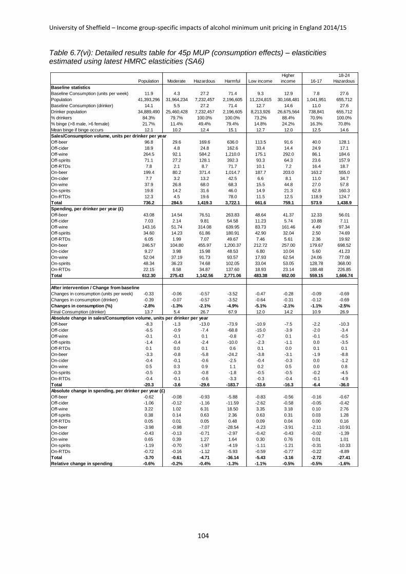
University of Sheffield – Income group-specific impacts of alcohol minimum unit pricing in England 2014/15
104
Table 6.7(vi): Detailed results table for 45p MUP (consumption effects) – elasticities estimated using latest HMRC elasticities (SA6)
Population Moderate Hazardous Harmful Low income
Higher
income 16-17
18-24
Hazardous
Baseline statistics
Baseline Consumption (units per week) 11.9 4.3 27.2 71.4 9.3 12.9 7.8 27.6
Population 41,393,296 31,964,234 7,232,457 2,196,605 11,224,815 30,168,481 1,041,951 655,712
Baseline Consumption (drinker) 14.1 5.5 27.2 71.4 12.7 14.6 11.0 27.6
Drinker population 34,889,490 25,460,428 7,232,457 2,196,605 8,213,926 26,675,564 738,841 655,712
% drinkers 84.3% 79.7% 100.0% 100.0% 73.2% 88.4% 70.9% 100.0%
% binge (>8 male, >6 female) 21.7% 11.4% 49.4% 79.4% 14.8% 24.2% 16.3% 70.8%
Mean binge if binge occurs 12.1 10.2 12.4 15.1 12.7 12.0 12.5 14.6
Sales/Consumption volume, units per drinker per year
Off-beer 96.8 29.6 169.6 636.0 113.5 91.6 40.0 128.1
Off-cider 18.9 4.8 24.8 162.6 33.4 14.4 24.9 17.1
Off-wine 264.5 92.1 584.2 1,210.0 175.1 292.0 86.1 184.6
Off-spirits 71.1 27.2 128.1 392.3 93.3 64.3 23.6 157.9
Off-RTDs 7.8 2.1 8.7 71.7 10.1 7.2 16.4 18.7
On-beer 199.4 80.2 371.4 1,014.7 187.7 203.0 163.2 555.0
On-cider 7.7 3.2 13.2 42.5 6.6 8.1 11.0 34.7
On-wine 37.9 26.8 68.0 68.3 15.5 44.8 27.0 57.8
On-spirits 19.8 14.2 31.6 46.0 14.9 21.3 62.8 160.3
On-RTDs 12.3 4.5 19.6 78.0 11.5 12.5 118.9 124.7
Total 736.2 284.5 1,419.3 3,722.1 661.6 759.1 573.9 1,438.9
Spending, per drinker per year (£)
Off-beer 43.08 14.54 76.51 263.83 48.64 41.37 12.33 56.01
Off-cider 7.03 2.14 9.81 54.58 11.23 5.74 10.88 7.11
Off-wine 143.16 51.74 314.08 639.95 83.73 161.46 4.49 97.34
Off-spirits 34.60 14.23 61.86 180.91 42.90 32.04 2.50 74.69
Off-RTDs 6.05 1.99 7.07 49.67 7.46 5.61 2.36 19.92
On-beer 246.57 104.80 455.97 1,200.37 212.72 257.00 179.67 698.52
On-cider 9.27 3.98 15.98 48.53 6.80 10.04 5.60 41.23
On-wine 52.04 37.19 91.73 93.57 17.93 62.54 24.06 77.08
On-spirits 48.34 36.23 74.68 102.05 33.04 53.05 128.78 368.00
On-RTDs 22.15 8.58 34.87 137.60 18.93 23.14 188.48 226.85
Total 612.30 275.43 1,142.56 2,771.06 483.38 652.00 559.15 1,666.74
After intervention / Change from baseline
Changes in consumption (units per week) -0.33 -0.06 -0.57 -3.52 -0.47 -0.28 -0.09 -0.69
Changes in consumption (drinker) -0.39 -0.07 -0.57 -3.52 -0.64 -0.31 -0.12 -0.69
Changes in consumption (%) -2.8% -1.3% -2.1% -4.9% -5.1% -2.1% -1.1% -2.5%
Final Consumption (drinker) 13.7 5.4 26.7 67.9 12.0 14.2 10.9 26.9
Absolute change in sales/Consumption volume, units per drinker per year
Off-beer -8.3 -1.3 -13.0 -73.9 -10.9 -7.5 -2.2 -10.3
Off-cider -6.5 -0.9 -7.4 -68.8 -15.0 -3.9 -2.0 -3.4
Off-wine -0.1 -0.1 0.1 -0.8 -0.7 0.1 -0.1 -0.5
Off-spirits -1.4 -0.4 -2.4 -10.0 -2.3 -1.1 0.0 -3.5
Off-RTDs 0.1 0.0 0.1 0.6 0.1 0.0 0.1 0.1
On-beer -3.3 -0.8 -5.8 -24.2 -3.8 -3.1 -1.9 -8.8
On-cider -0.4 -0.1 -0.6 -2.5 -0.4 -0.3 0.0 -1.2
On-wine 0.5 0.3 0.9 1.1 0.2 0.5 0.0 0.8
On-spirits -0.5 -0.3 -0.8 -1.8 -0.5 -0.5 -0.2 -4.5
On-RTDs -0.4 -0.1 -0.6 -3.3 -0.3 -0.4 -0.1 -4.9
Total -20.3 -3.6 -29.6 -183.7 -33.6 -16.3 -6.4 -36.0
Absolute change in spending, per drinker per year (£)
Off-beer -0.62 -0.08 -0.93 -5.88 -0.83 -0.56 -0.16 -0.67
Off-cider -1.06 -0.12 -1.16 -11.59 -2.62 -0.58 -0.05 -0.42
Off-wine 3.22 1.02 6.31 18.50 3.35 3.18 0.10 2.76
Off-spirits 0.38 0.14 0.63 2.36 0.63 0.31 0.03 1.28
Off-RTDs 0.05 0.01 0.05 0.48 0.09 0.04 0.00 0.16
On-beer -3.98 -0.98 -7.07 -28.54 -4.23 -3.91 -2.11 -10.91
On-cider -0.43 -0.13 -0.71 -2.97 -0.42 -0.43 -0.02 -1.39
On-wine 0.65 0.39 1.27 1.64 0.30 0.76 0.01 1.01
On-spirits -1.19 -0.70 -1.97 -4.19 -1.11 -1.21 -0.31 -10.33
On-RTDs -0.72 -0.16 -1.12 -5.93 -0.59 -0.77 -0.22 -8.89
Total -3.70 -0.61 -4.71 -36.14 -5.43 -3.16 -2.72 -27.41
Relative change in spending -0.6% -0.2% -0.4% -1.3% -1.1% -0.5% -0.5% -1.6%


![Adolescent Alcohol Exposure Persistently Impacts …pharmrev.aspetjournals.org/.../pharmrev/68/4/1074.full.pdfAA019767, AA11605, AA007573, and AA021040], Neurobiology of Adolescent](https://static.fdocuments.in/doc/165x107/5f0f015d7e708231d4420425/adolescent-alcohol-exposure-persistently-impacts-aa019767-aa11605-aa007573-and.jpg)