ModelingBasketball FreeThrowsfaculty.ccri.edu/joallen/M2910/Modeling Basketball Free Throws.pdf ·...
24
SIAM REVIEW c 2005 Society for Industrial and Applied Mathematics Vol. 47, No. 4, pp. 775–798 Modeling Basketball Free Throws ∗ Joerg M. Gablonsky † Andrew S. I. D. Lang ‡ Abstract. This paper presents a mathematical model for basketball free throws. It is intended to be a supplement to an existing calculus course and could easily be used as a basis for a calculus project. Students will learn how to apply calculus to model an interesting real-world problem, from problem identification all the way through to interpretation and verification. Along the way we will introduce topics such as optimization (univariate and multiobjective), numerical methods, and differential equations. Key words. basketball, mathematical modeling, calculus projects AMS subject classifications. 00-01, 00A71, 26A06 DOI. 10.1137/S0036144598339555 1. Introduction. In these days of superstar basketball players, you would think that shooting free throws should be as much a formality, and just as exciting, as the extra point in professional football. Not so. Take for example Shaquille O’Neal, the subject of our first model, who as of the end of the 2004–2005 regular season had a career free throw percentage of 53.1%. His troubles seemed to increase during the playoffs, where he shot around 45% from the line. Shaquille is not alone in his free throw shooting troubles. In fact nearly one-third of all NBA players shoot less than 70% from the foul line. When a basketball player steps up to shoot a free throw he does not usually think (unless he also happens to be a mathematician), “I wonder if my free throw shooting percentage would improve if I changed my initial shooting angle,” or “I wonder how air resistance affects the trajectory of my shot,” or even “Should I be aiming for the back rim, front rim, or the middle of the basket?” We present here a calculus-based model for basketball free throws to show that they should address some of these musings. We begin by conjecturing that some players shoot poorly from the line because they are shooting the ball at the wrong angle. Therefore, the focus of our model will be the release angle, a simple place to start, and we will extend it later. Some of the more interesting facts that we’ll discover by refining and interpreting our model are: 1. The best way to shoot free throws depends upon the person shooting. The two most important factors are their height and ∗ Received by the editors May 22, 1998; accepted for publication (in revised form) July 20, 2005; published electronically October 31, 2005. http://www.siam.org/journals/sirev/47-4/33955.html † The Boeing Company, Mathematics and Engineering Analysis, P.O. Box 3707, MC 7L-21, Seat- tle, WA 98124-2207 ([email protected]). ‡ Department of Computer Science and Mathematics, Oral Roberts University, 7777 South Lewis Ave., Tulsa, OK 74171 ([email protected]). 775
Transcript of ModelingBasketball FreeThrowsfaculty.ccri.edu/joallen/M2910/Modeling Basketball Free Throws.pdf ·...
SIAM REVIEW c© 2005 Society for Industrial and Applied MathematicsVol. 47, No. 4, pp. 775–798
Modeling BasketballFree Throws∗
Joerg M. Gablonsky†
Andrew S. I. D. Lang‡
Abstract. This paper presents a mathematical model for basketball free throws. It is intended tobe a supplement to an existing calculus course and could easily be used as a basis fora calculus project. Students will learn how to apply calculus to model an interestingreal-world problem, from problem identification all the way through to interpretation andverification. Along the way we will introduce topics such as optimization (univariate andmultiobjective), numerical methods, and differential equations.
Key words. basketball, mathematical modeling, calculus projects
AMS subject classifications. 00-01, 00A71, 26A06
DOI. 10.1137/S0036144598339555
1. Introduction. In these days of superstar basketball players, you would thinkthat shooting free throws should be as much a formality, and just as exciting, as theextra point in professional football. Not so. Take for example Shaquille O’Neal, thesubject of our first model, who as of the end of the 2004–2005 regular season had acareer free throw percentage of 53.1%. His troubles seemed to increase during theplayoffs, where he shot around 45% from the line. Shaquille is not alone in his freethrow shooting troubles. In fact nearly one-third of all NBA players shoot less than70% from the foul line.
When a basketball player steps up to shoot a free throw he does not usually think(unless he also happens to be a mathematician), “I wonder if my free throw shootingpercentage would improve if I changed my initial shooting angle,” or “I wonder how airresistance affects the trajectory of my shot,” or even “Should I be aiming for the backrim, front rim, or the middle of the basket?” We present here a calculus-based modelfor basketball free throws to show that they should address some of these musings.We begin by conjecturing that some players shoot poorly from the line because theyare shooting the ball at the wrong angle. Therefore, the focus of our model will bethe release angle, a simple place to start, and we will extend it later. Some of themore interesting facts that we’ll discover by refining and interpreting our model are:
1. The best way to shoot free throws depends upon the personshooting. The two most important factors are their height and
∗Received by the editors May 22, 1998; accepted for publication (in revised form) July 20, 2005;published electronically October 31, 2005.
http://www.siam.org/journals/sirev/47-4/33955.html†The Boeing Company, Mathematics and Engineering Analysis, P.O. Box 3707, MC 7L-21, Seat-
tle, WA 98124-2207 ([email protected]).‡Department of Computer Science and Mathematics, Oral Roberts University, 7777 South Lewis
Ave., Tulsa, OK 74171 ([email protected]).
775
776 JOERG M. GABLONSKY AND ANDREW S. I. D. LANG
how consistent they are in controlling both the release angle andthe release velocity.
2. In general, the taller you are, the lower your release angle shouldbe. We’ll actually see that taller players are allowed more errorin both their release angles and release velocities and thus theyshould have an easier time shooting free throws than shorter players.
3. It is much more important to consistently use the right releasevelocity than the right release angle.
4. The best shot does not pass through the center of the hoop. The besttrajectories pass through the hoop somewhere between the centerand the back rim. Taller players should shoot closer to the centerwhile shorter players should aim more towards the back rim.
2. Mathematical Modeling. Before we jump into modeling a basketball freethrow, it would help for us to tell you exactly what we mean by mathematical mod-eling:
Mathematical modeling is the process of formulatingreal world situations in mathematical terms.
Less formally, mathematical modeling takes observed real-world behaviors or phe-nomena and describes them using mathematical formulae or equations. All the formu-lae you see in your physics, chemistry, and biology classes are mathematical models.Mathematical models can be found everywhere, not only in science, but also in thesocial sciences and even in business. For instance, there are people who get paid verywell to model the stock market. By constructing mathematical models, we can oftenexplain real-world behavior, predict how sensitive real-world situations are to certainchanges, and even predict future behavior (very useful for the people who model thestock market). The following is a summary of the standard steps for constructing amathematical model:
1. Identify the problem. What do you want to find out?2. Derive the model. Identify the constants and variables involved.
Make assumptions about which variables to include in the model.Determine the interrelationships between the variables.
3. Solve the equations and interpret the model.4. Verify the model. Does it answer the original problem? Does it
match up to real-world data?5. Refine the model. If the model is not satisfactory, refine it by
removing some of your earlier assumptions.
We’ll discuss these steps in greater detail as we use them to model basketball freethrows.
3. Our First Model: The Best Angle. It is true for most models, including ours,that trying to include every possible physical effect immediately is rather ambitious,especially if you want to be able to solve the model. The modeling process typicallybegins with the construction of very simple models which are easy to solve. Modelsare then refined to make them more realistic, which in turn requires the introductionof more powerful mathematics in order to solve them. In the end the model should
MODELING BASKETBALL FREE THROWS 777
Table 3.1 The physical constants of the problem.
Physical constant Symbol Value
Rim diameter Dr 1.5 ft
Ball diameter Db 0.8 ft
Horizontal distance traversed l 13 ft 6.5 in
Vertical distance traversed h 1 ft 1 34 in
Acceleration due to gravity g −32 ft s−2
be refined enough to describe reality as closely as possible while still being solvable.You’ll see this refinement process in action as we go through the modeling procedure.
3.1. Problem Definition. When watching basketball players shoot free throwswe notice that sometimes they make small errors and still make the basket. It seemsreasonable that the amount of error that the player can make and still have the shotgo in depends on the initial angle that the ball was thrown. We’ll therefore begin bydefining the problem as follows:
Given a basketball player of a certain height,what is the best angle for him to shoot a free throw.
3.2. Deriving Our First Model: Identify the Constants and Variables. Thephysical constants (the diameter of the rim, etc.) that we shall use to derive the equa-tions of motion that govern the flight of the ball can be obtained from various sources,including the Internet, books [14, 17], and actual (tape measure) measurements. Thediameter of the rim, Dr, is 1.5 ft. The diameter of the ball, Db, is taken to be 0.8 ft.1
It has been observed [7] that free throws are shot from a few inches in front ofthe free throw line. We thus take the horizontal distance traversed, l, to be 13’6.5”rather than the total distance, 14’, from the free throw line to the center of the hoop.It has also been observed [4, 8, 19] that shooters release the ball, on average, from aheight of approximately 1.25 times the shooter’s own height. For example, a 7’1” tallplayer releases the ball, on average, at a height of approximately 8’101
4”. Thus, fora 7’1” tall player, we would take the net vertical distance traversed, h, to be 1’1 3
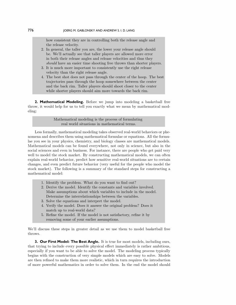
4”.See Table 3.1 and Figure 3.1.
3.3. Deriving Our First Model: Simplifying Assumptions. We make the fol-lowing simplifying assumptions for our first model:
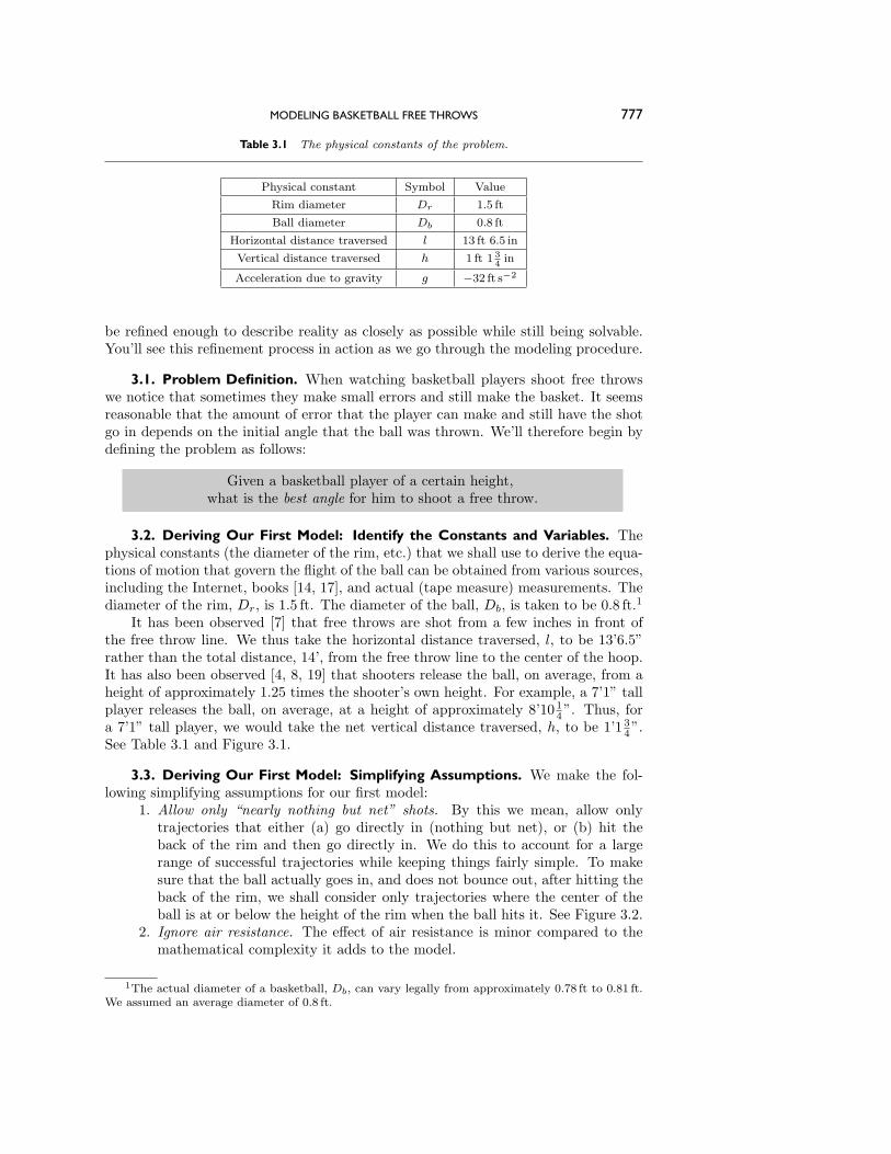
1. Allow only “nearly nothing but net” shots. By this we mean, allow onlytrajectories that either (a) go directly in (nothing but net), or (b) hit theback of the rim and then go directly in. We do this to account for a largerange of successful trajectories while keeping things fairly simple. To makesure that the ball actually goes in, and does not bounce out, after hitting theback of the rim, we shall consider only trajectories where the center of theball is at or below the height of the rim when the ball hits it. See Figure 3.2.
2. Ignore air resistance. The effect of air resistance is minor compared to themathematical complexity it adds to the model.
1The actual diameter of a basketball, Db, can vary legally from approximately 0.78 ft to 0.81 ft.We assumed an average diameter of 0.8 ft.
778 JOERG M. GABLONSKY AND ANDREW S. I. D. LANG
Fig. 3.1 The conceptualization of the free throw.
Fig. 3.2 Ball going in off the back of the rim.
3. Ignore any spin the ball may have. Spin becomes important if we allow theball to bounce before it goes in. Since we are only allowing nearly nothingbut net shots, and ignoring air resistance, we’ll also ignore spin.
4. There is no sideways error in the trajectory. If you want to be a good freethrow shooter, you really ought to shoot straight. The benefit we get fromassuming the shooter always shoots straight is that the model will be two-dimensional (constrained to a plane). If transverse error were to be included,the model would be a more realistic, but harder to solve, three-dimensionalone.
5. There is no error in the initial shooting velocity. We are assuming thatsome basketball players have problems shooting free throws because they areshooting at the wrong angle. Therefore, our first model concentrates on errorsin the release angle only.
6. The best shot is one that goes through the center of the hoop. That is, themodel will be one in which the initial velocity is the velocity that would dropthe center of the ball through the center of the hoop. Some coaches encouragethis by placing an insert into the ring that makes the aperture smaller.
7. The shooter is 7’1” tall. After we find the best angle for Shaq, we will quicklyremove this assumption and find the best angle for people of a more diminutivestature.
MODELING BASKETBALL FREE THROWS 779
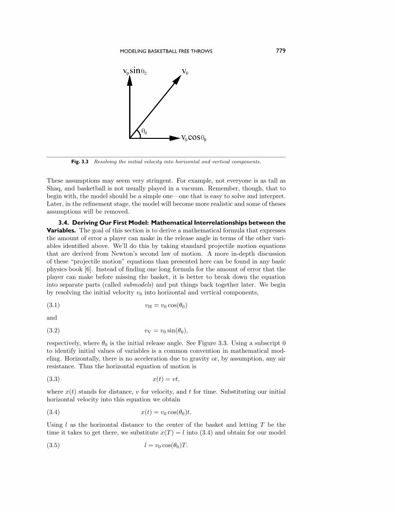
Fig. 3.3 Resolving the initial velocity into horizontal and vertical components.
These assumptions may seem very stringent. For example, not everyone is as tall asShaq, and basketball is not usually played in a vacuum. Remember, though, that tobegin with, the model should be a simple one—one that is easy to solve and interpret.Later, in the refinement stage, the model will become more realistic and some of thesesassumptions will be removed.
3.4. Deriving Our First Model: Mathematical Interrelationships between theVariables. The goal of this section is to derive a mathematical formula that expressesthe amount of error a player can make in the release angle in terms of the other vari-ables identified above. We’ll do this by taking standard projectile motion equationsthat are derived from Newton’s second law of motion. A more in-depth discussionof these “projectile motion” equations than presented here can be found in any basicphysics book [6]. Instead of finding one long formula for the amount of error that theplayer can make before missing the basket, it is better to break down the equationinto separate parts (called submodels) and put things back together later. We beginby resolving the initial velocity v0 into horizontal and vertical components,
vH = v0 cos(θ0)(3.1)
and
vV = v0 sin(θ0),(3.2)
respectively, where θ0 is the initial release angle. See Figure 3.3. Using a subscript 0to identify initial values of variables is a common convention in mathematical mod-eling. Horizontally, there is no acceleration due to gravity or, by assumption, any airresistance. Thus the horizontal equation of motion is
x(t) = vt,(3.3)
where x(t) stands for distance, v for velocity, and t for time. Substituting our initialhorizontal velocity into this equation we obtain
x(t) = v0 cos(θ0)t.(3.4)
Using l as the horizontal distance to the center of the basket and letting T be thetime it takes to get there, we substitute x(T ) = l into (3.4) and obtain for our model
l = v0 cos(θ0)T.(3.5)
780 JOERG M. GABLONSKY AND ANDREW S. I. D. LANG
Similarly, the vertical equation of motion is given by
y(t) = vt+12gt2 = v0 sin(θ0)t+
12gt2,(3.6)
where g = −32 ft s−2(−9.8 m s−2) is the acceleration due to gravity. Substitutingy(T ) = h, the vertical distance to the center of the basket, into the above equation,we obtain for our model
h = v0 sin(θ0)T +12gT 2,(3.7)
where h is the vertical distance to the center of the basket. Solving (3.5) for T ,
T =l
cos(θ0)v0,(3.8)
and substituting it into (3.7), we find the initial velocity v0 needed, for a given initialangle θ0, so that the basketball goes through the middle of the hoop:
v0 =l
cos θ0
√−g
2 (l tan (θ0)− h).(3.9)
We note that this formula gives us sensible answers only for a limited range of θ0.Not only does it physically make sense to restrict initial angles to ones that resultin forward motion, i.e., 0 < θ0 < 90◦, but also notice that the formula gives realvalues only for l tan(θ0)− h > 0 (remember g is negative). Physically this inequalitycorresponds to the ball having a sufficiently high initial release angle to reach theheight of the rim. Thus we take the range of initial release angles to be tan−1
(hl
)<
θ0 < 90◦.
In modeling, it is always good practice to note the range that yourparameters can take. Otherwise you may unwittingly attain
solutions which turn out to be nonphysical.
We make special note of the physical range of θ0 here, because it is important forthe numerical methods used to find solutions later in this paper. Furthermore, notethat we assume that the ball will not hit the front of the rim on trajectories wherethe ball passes through the center of the hoop. We will show later that this mightnot be true, especially for shorter players.
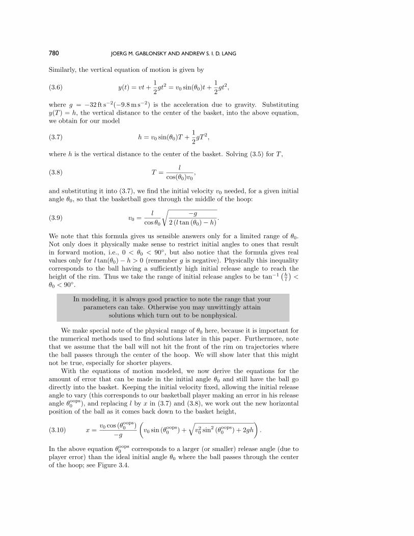
With the equations of motion modeled, we now derive the equations for theamount of error that can be made in the initial angle θ0 and still have the ball godirectly into the basket. Keeping the initial velocity fixed, allowing the initial releaseangle to vary (this corresponds to our basketball player making an error in his releaseangle θoops
0 ), and replacing l by x in (3.7) and (3.8), we work out the new horizontalposition of the ball as it comes back down to the basket height,
x =v0 cos (θoops
0 )−g
(v0 sin (θoops
0 ) +√v2
0 sin2 (θoops0 ) + 2gh
).(3.10)
In the above equation θoops0 corresponds to a larger (or smaller) release angle (due to
player error) than the ideal initial angle θ0 where the ball passes through the centerof the hoop; see Figure 3.4.
MODELING BASKETBALL FREE THROWS 781
Fig. 3.4 Comparison of the ideal trajectory that passes through the center on the hoop (v0, θ0) (red)and the trajectory with an error in the release angle (v0, θ
oops0 ) (blue).
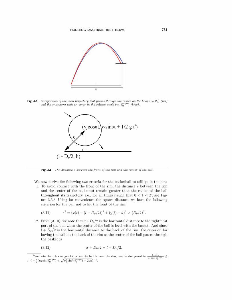
Fig. 3.5 The distance s between the front of the rim and the center of the ball.
We now derive the following two criteria for the basketball to still go in the net:1. To avoid contact with the front of the rim, the distance s between the rim
and the center of the ball must remain greater than the radius of the ballthroughout its trajectory, i.e., for all times t such that 0 < t < T ; see Fig-ure 3.5.2 Using for convenience the square distance, we have the followingcriterion for the ball not to hit the front of the rim:
s2 = (x(t)− (l −Dr/2))2 + (y(t)− h)2 > (Db/2)2.(3.11)
2. From (3.10), we note that x+Db/2 is the horizontal distance to the rightmostpart of the ball when the center of the ball is level with the basket. And sincel + Dr/2 is the horizontal distance to the back of the rim, the criterion forhaving the ball hit the back of the rim as the center of the ball passes throughthe basket is
x+Db/2 = l +Dr/2.(3.12)
2We note that this range of t, when the ball is near the rim, can be sharpened to l−Drv0 cos(θoops
0 )≤
t ≤ − 1g(v0 sin(θ
oops0 ) +
√v20 sin
2(θoops0 ) + 2gh)−1.
782 JOERG M. GABLONSKY AND ANDREW S. I. D. LANG
3.5. Solving the Equations. To find the error allowed for a given initial angleθ0, we keep v0 fixed and solve numerically for the unique release angles θlow < θ0 andθhigh > θ0, which are, respectively, the solutions to the following equations:
s2 − (Db/2)2 = 0,(3.13)
the ball is released at an angle lower than θ0 and just misses the front of the rim asit goes in, and
x− l +Db −Dr
2= 0,(3.14)
the ball is released at a angle higher than θ0 and hits the back of the rim and goesin. We note here that increasing the initial angle may increase xh, the distance tothe center of the ball as it passes through the center of the hoop, but after a certainpoint xh will start to decrease. This can happen before the ball hits the back of therim. So for certain trajectories, there is no solution to (3.14) and both θlow and θhighare solutions to (3.13). This behavior will be made more apparent in the next fewsections. After solving for θlow and θhigh, we find the minimum deviation from θ0,
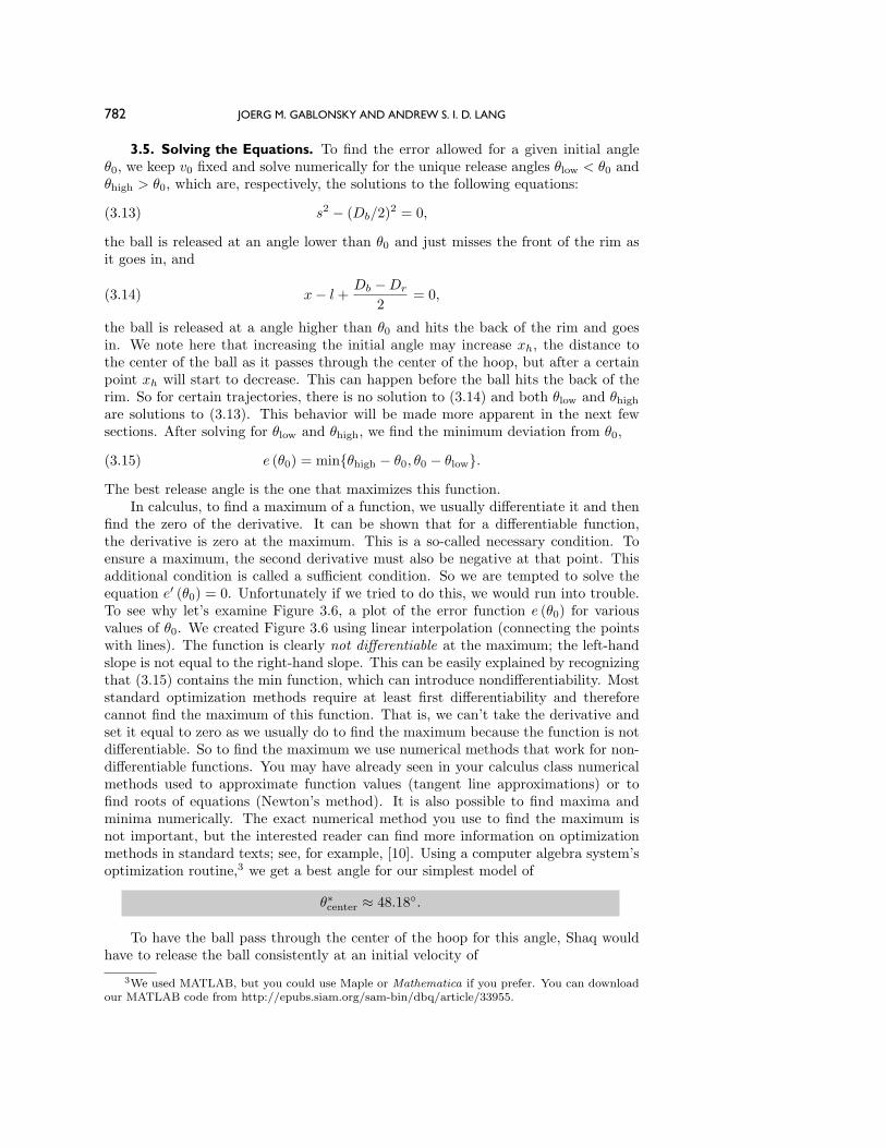
e (θ0) = min{θhigh − θ0, θ0 − θlow}.(3.15)
The best release angle is the one that maximizes this function.In calculus, to find a maximum of a function, we usually differentiate it and then
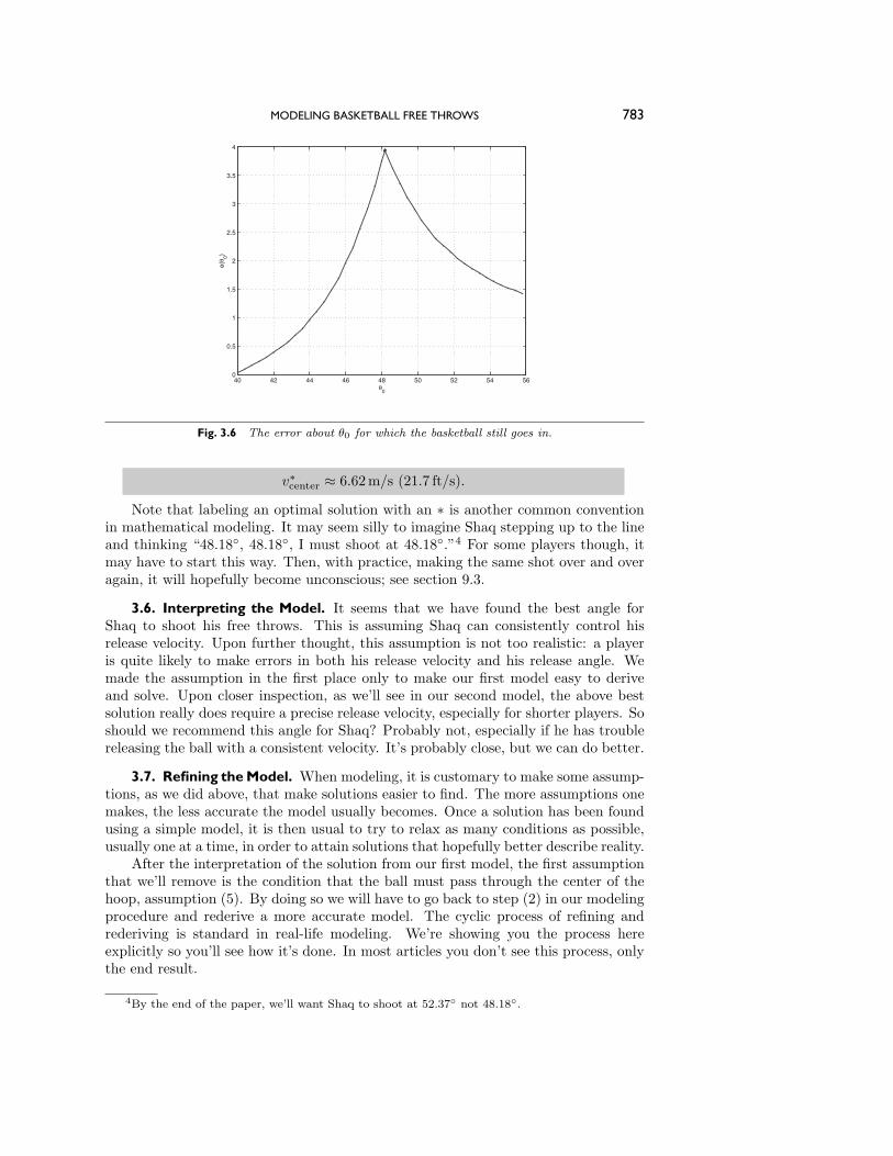
find the zero of the derivative. It can be shown that for a differentiable function,the derivative is zero at the maximum. This is a so-called necessary condition. Toensure a maximum, the second derivative must also be negative at that point. Thisadditional condition is called a sufficient condition. So we are tempted to solve theequation e′ (θ0) = 0. Unfortunately if we tried to do this, we would run into trouble.To see why let’s examine Figure 3.6, a plot of the error function e (θ0) for variousvalues of θ0. We created Figure 3.6 using linear interpolation (connecting the pointswith lines). The function is clearly not differentiable at the maximum; the left-handslope is not equal to the right-hand slope. This can be easily explained by recognizingthat (3.15) contains the min function, which can introduce nondifferentiability. Moststandard optimization methods require at least first differentiability and thereforecannot find the maximum of this function. That is, we can’t take the derivative andset it equal to zero as we usually do to find the maximum because the function is notdifferentiable. So to find the maximum we use numerical methods that work for non-differentiable functions. You may have already seen in your calculus class numericalmethods used to approximate function values (tangent line approximations) or tofind roots of equations (Newton’s method). It is also possible to find maxima andminima numerically. The exact numerical method you use to find the maximum isnot important, but the interested reader can find more information on optimizationmethods in standard texts; see, for example, [10]. Using a computer algebra system’soptimization routine,3 we get a best angle for our simplest model of
θ∗center ≈ 48.18◦.
To have the ball pass through the center of the hoop for this angle, Shaq wouldhave to release the ball consistently at an initial velocity of
3We used MATLAB, but you could use Maple or Mathematica if you prefer. You can downloadour MATLAB code from http://epubs.siam.org/sam-bin/dbq/article/33955.
MODELING BASKETBALL FREE THROWS 783
40 42 44 46 48 50 52 54 560
0.5
1
1.5
2
2.5
3
3.5
4
e(θ 0)
θ0
Fig. 3.6 The error about θ0 for which the basketball still goes in.
v∗center ≈ 6.62 m/s (21.7 ft/s).
Note that labeling an optimal solution with an ∗ is another common conventionin mathematical modeling. It may seem silly to imagine Shaq stepping up to the lineand thinking “48.18◦, 48.18◦, I must shoot at 48.18◦.”4 For some players though, itmay have to start this way. Then, with practice, making the same shot over and overagain, it will hopefully become unconscious; see section 9.3.
3.6. Interpreting the Model. It seems that we have found the best angle forShaq to shoot his free throws. This is assuming Shaq can consistently control hisrelease velocity. Upon further thought, this assumption is not too realistic: a playeris quite likely to make errors in both his release velocity and his release angle. Wemade the assumption in the first place only to make our first model easy to deriveand solve. Upon closer inspection, as we’ll see in our second model, the above bestsolution really does require a precise release velocity, especially for shorter players. Soshould we recommend this angle for Shaq? Probably not, especially if he has troublereleasing the ball with a consistent velocity. It’s probably close, but we can do better.
3.7. Refining theModel. When modeling, it is customary to make some assump-tions, as we did above, that make solutions easier to find. The more assumptions onemakes, the less accurate the model usually becomes. Once a solution has been foundusing a simple model, it is then usual to try to relax as many conditions as possible,usually one at a time, in order to attain solutions that hopefully better describe reality.
After the interpretation of the solution from our first model, the first assumptionthat we’ll remove is the condition that the ball must pass through the center of thehoop, assumption (5). By doing so we will have to go back to step (2) in our modelingprocedure and rederive a more accurate model. The cyclic process of refining andrederiving is standard in real-life modeling. We’re showing you the process hereexplicitly so you’ll see how it’s done. In most articles you don’t see this process, onlythe end result.
4By the end of the paper, we’ll want Shaq to shoot at 52.37◦ not 48.18◦.
784 JOERG M. GABLONSKY AND ANDREW S. I. D. LANG
4. Our Second Model. The Best Trajectory. Let’s improve our model by re-moving the assumption that the best shot is one where the ball goes through thecenter of the hoop. Still keeping the same equations of motion, and sticking with our7’1” basketball player, we now let both the initial velocity v0 and the initial angleθ0 vary independently and at the same time. Each pair (v0, θ0) will give the ball atrajectory that results in either a made basket or a missed basket.
4.1. Is There a Better Target Than the Center? Constructing a FeasibleRegion. Again, the model function is not differentiable, so simple calculus fails ushere, and a numerical investigation is needed:
The feasible region of trajectories is theset of all pairs (v0, θ0) that result in a successful free throw
(using the assumptions on allowable trajectories).
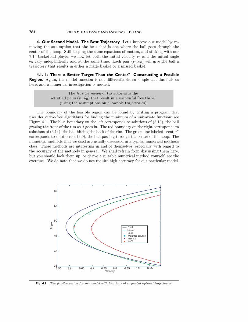
The boundary of the feasible region can be found by writing a program thatuses derivative-free algorithms for finding the minimum of a univariate function; seeFigure 4.1. The blue boundary on the left corresponds to solutions of (3.13), the ballgrazing the front of the rim as it goes in. The red boundary on the right corresponds tosolutions of (3.14), the ball hitting the back of the rim. The green line labeled “center”corresponds to solutions of (3.9), the ball passing through the center of the hoop. Thenumerical methods that we used are usually discussed in a typical numerical methodsclass. These methods are interesting in and of themselves, especially with regard tothe accuracy of the methods in general. We shall refrain from discussing them here,but you should look them up, or derive a suitable numerical method yourself; see theexercises. We do note that we do not require high accuracy for our particular model.
60
55
50
45
40
356.55 6.6 6.65 6.7 6.75 6.8 6.85 6.9 6.95
Velocity
Ang
le
FrontCenterBackWeighted solutionMax
0 0
Fig. 4.1 The feasible region for our model with locations of suggested optimal trajectories.
MODELING BASKETBALL FREE THROWS 785
Looking at the previous solution location in the feasible region, the red × onFigure 4.1, we see that requiring the ball to pass through the center of the hoopmay not be best. There is much more room to overshoot than to undershoot. Thistrajectory would be good for a person who, when they missed, missed by consistentlyovershooting, but for someone who consistently undershoots when they miss thistrajectory is definitely not best. What we have discovered here is that
What we should consider best depends uponthe individual and the way they shoot.
What pairs (v0, θ0) allow for the largest error in angle? If we let the ball gothrough the hoop at any position and maximize the allowed error in initial angle, weobtain the point marked with a dot on Figure 4.1. We see that this candidate optimaltrajectory corresponds to a maximum allowable error in θ0 but no allowable error inv0; see also [2]. The combination that maximizes the amount of allowable error inthe velocity is not as easy to find. It turns out that increasing the release angle alsoincreases the allowable error in velocity. This continues until the release angle to hitthe front and back of the rim for a given velocity are equal; i.e., this rainbow shothas no allowable error in the release angle; see Figure 4.2. Such a high angle, highvelocity shot may not be physically possible to shoot. We may not be strong enoughor we may hit the ceiling! The third point marked with a blue + on Figure 4.1 willbe discussed later.
As we pointed out earlier, formula (3.9) is valid only in a certain range. Figure 4.1shows that at a low release angle (i.e., an angle below the intersection point of thegreen and blue curves), the velocity given by (3.9) would lead to trajectories where theball would pass through the rim before reaching the center of the hoop. This means
If you have a shallow shot, don’t aim for the center of the basketbecause you’ll hit the front rim and probably miss.
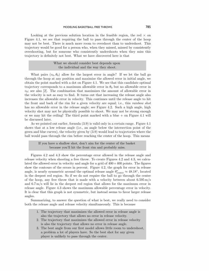
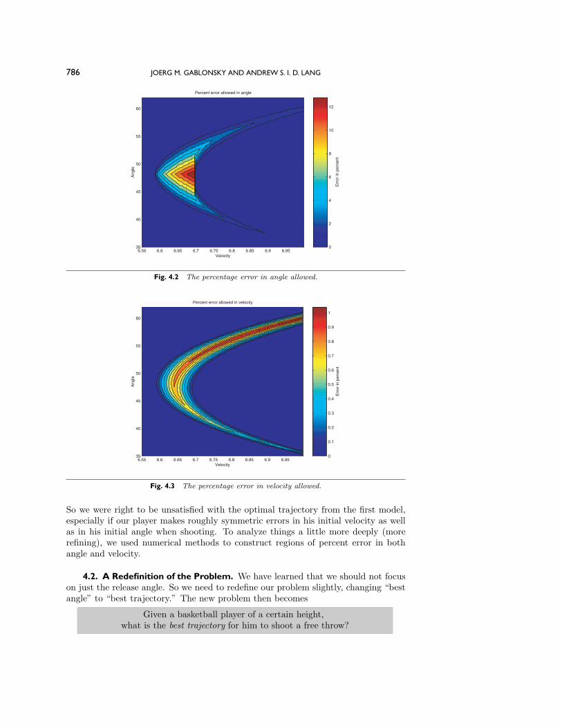
Figures 4.2 and 4.3 show the percentage error allowed in the release angle andrelease velocity when shooting a free throw. To create Figures 4.2 and 4.3, we calcu-lated the allowed error in velocity and angle for a grid of 400×400 points. The figuresshow the contours of the errors in percent. Figure 4.2, the graph for error in releaseangle, is nearly symmetric around the optimal release angle θ∗center ≈ 48.18◦, locatedin the deepest red region. So if we do not require the ball to go through the centerof the hoop, any free throw that is made with a velocity between about 6.595 m/sand 6.7 m/s will lie in the deepest red region that allows for the maximum error inrelease angle. Figure 4.3 shows the maximum allowable percentage error in velocity.It is clear that this graph is not symmetric, but instead seems to favor larger releaseangles.
Summarizing, to answer the question of what is best, we really need to considerboth the release angle and release velocity simultaneously. This is because
1. The trajectory that maximizes the allowed error in release angle isalso the trajectory that allows no error in release velocity.
2. The trajectory that maximizes the allowed error in release velocityis also the trajectory that allows no error in release angle.
3. The best angle from our first model allows little room to undershoot,a problem a lot of players have. So the best shot for any givenplayer is unlikely to pass through the center.
786 JOERG M. GABLONSKY AND ANDREW S. I. D. LANG
6.55 6.6 6.65 6.7 6.75 6.8 6.85 6.9 6.9535
40
45
50
55
60
Percent error allowed in angle
Velocity
Ang
le
Err
or in
per
cent
0
2
4
6
8
10
12
Fig. 4.2 The percentage error in angle allowed.
6.55 6.6 6.65 6.7 6.75 6.8 6.85 6.9 6.9535
40
45
50
55
60
Percent error allowed in velocity
Velocity
Ang
le
Err
or in
per
cent
0
0.1
0.2
0.3
0.4
0.5
0.6
0.7
0.8
0.9
1
Fig. 4.3 The percentage error in velocity allowed.
So we were right to be unsatisfied with the optimal trajectory from the first model,especially if our player makes roughly symmetric errors in his initial velocity as wellas in his initial angle when shooting. To analyze things a little more deeply (morerefining), we used numerical methods to construct regions of percent error in bothangle and velocity.
4.2. A Redefinition of the Problem. We have learned that we should not focuson just the release angle. So we need to redefine our problem slightly, changing “bestangle” to “best trajectory.” The new problem then becomes
Given a basketball player of a certain height,what is the best trajectory for him to shoot a free throw?
MODELING BASKETBALL FREE THROWS 787
Since the units of degrees and feet per second (or meters per second) are notdirectly relatable, the question of what we mean by “best trajectory” must also beclarified. One way to allow a comparison between the two different errors is by lookingat the percentage error. That is, relative to the velocity and angle with which theplayer wants to throw the ball, how much error can he make percentagewise and stillmake the free throw? Figures 4.2 and 4.3 already show the error in this measure.From this it is obvious that the percent error in angle can be much larger than thepercent error in velocity. Another conclusion we can therefore make is that
It is much more important to use the right velocityas compared to the right angle.
How do we find the optimal solution when we have two different measures wewant to minimize, and the two of them oppose each other? Problems of this kindare called multiobjective optimization problems, and there are many different waysto solve them.5
One way to solve the multiobjective problem is by fixing the angle that allowsthe largest error for many velocities and then maximizing the error in velocity. Thisresults in the point marked with a dot in Figure 4.1. Note again that this workedonly because we could decouple the two optimizations.
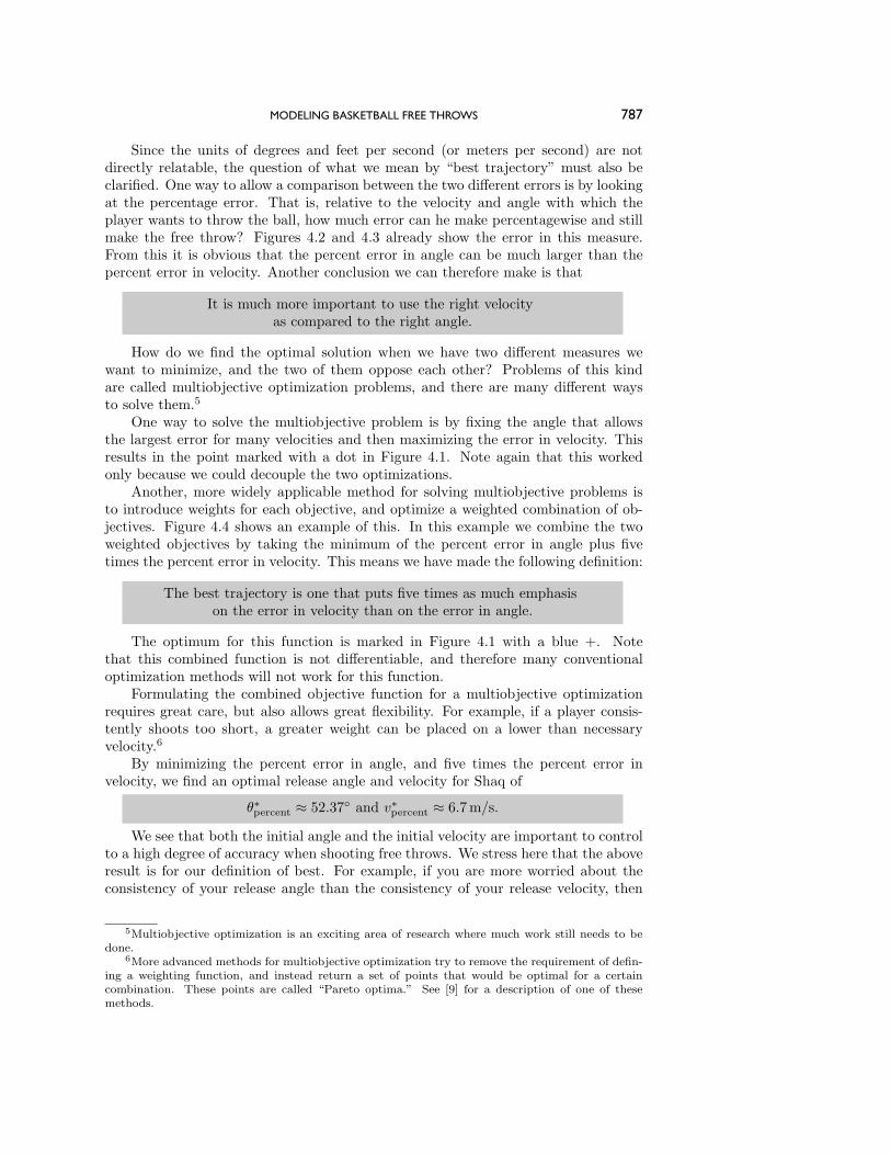
Another, more widely applicable method for solving multiobjective problems isto introduce weights for each objective, and optimize a weighted combination of ob-jectives. Figure 4.4 shows an example of this. In this example we combine the twoweighted objectives by taking the minimum of the percent error in angle plus fivetimes the percent error in velocity. This means we have made the following definition:
The best trajectory is one that puts five times as much emphasison the error in velocity than on the error in angle.
The optimum for this function is marked in Figure 4.1 with a blue +. Notethat this combined function is not differentiable, and therefore many conventionaloptimization methods will not work for this function.
Formulating the combined objective function for a multiobjective optimizationrequires great care, but also allows great flexibility. For example, if a player consis-tently shoots too short, a greater weight can be placed on a lower than necessaryvelocity.6
By minimizing the percent error in angle, and five times the percent error invelocity, we find an optimal release angle and velocity for Shaq of
θ∗percent ≈ 52.37◦ and v∗percent ≈ 6.7 m/s.
We see that both the initial angle and the initial velocity are important to controlto a high degree of accuracy when shooting free throws. We stress here that the aboveresult is for our definition of best. For example, if you are more worried about theconsistency of your release angle than the consistency of your release velocity, then
5Multiobjective optimization is an exciting area of research where much work still needs to bedone.
6More advanced methods for multiobjective optimization try to remove the requirement of defin-ing a weighting function, and instead return a set of points that would be optimal for a certaincombination. These points are called “Pareto optima.” See [9] for a description of one of thesemethods.
788 JOERG M. GABLONSKY AND ANDREW S. I. D. LANG
6.55 6.6 6.65 6.7 6.75 6.8 6.85 6.9 6.9535
40
45
50
55
60
Weighted error
Velocity
Ang
le
Wei
ghte
d er
ror
0
0.5
1
1.5
2
2.5
3
3.5
4
Fig. 4.4 The weighted error.
less weight should be placed on error in velocity as compared to error in angle. Thiswould result in a slightly lower θ∗percent (by a degree or two). Similarly someone whohas serious trouble shooting with a consistent release velocity should release the ballat a slightly higher angle than the average shooter.
In fact it is clearly evident that the optimal trajectory should be decided player byplayer according to whether the player consistently has more trouble controlling hisinitial velocity or his initial angle. Even players who, when they miss, miss consistentlyby shooting too short (like Shaq) can be accounted for.7
5. Our Third Model: Including Air Resistance. So far our model has excludedair resistance. This is because free throws have relatively low velocities and shorttravel times. It is also hard to do. The effect of air resistance, though, still needsto be considered in any full treatment. Hamilton and Reinschmidt [7] qualitativelydiscussed the inclusion of air resistance and suggested that any derived optimal releaseangles would be lower by about 2◦. This turns out to be an overestimate, as we’llsoon see.
5.1. Air Resistance. Motion with air resistance is usually discussed extensivelyin an introductory differential equations class. For a particularly good module see [3].
As the basketball travels through the air as it heads towards the basket, a force(viscous drag) that opposes the direction of motion arises due to air resistance. Thisforce is proportional to the velocity of the ball at each instant:
Fviscous = kv = 3πµDbv,(5.1)
where µ = 1.2165 ∗ 10−5 lb/(ft s) is the viscosity of air at 20◦C and 1 atm, and Db =0.8 ft is the diameter of the basketball. This gives a value of k = 9.172 ∗ 10−5 lb/sfor our model. We are making assumptions here about temperature, pressure, andhumidity. If we find out that air resistance is very important, we will have to be moreprecise here in order to better match reality. Think Denver Nuggets.
7In our opinion Shaq misses because he shoots at too low a release angle and has erratic velocitycontrol; see the last exercise.
MODELING BASKETBALL FREE THROWS 789
5.2. Our Third Model: Revised Equations of Motion. We now go back to step(2) in our modeling procedure and rederive the equations of motion. Assuming theball is released with initial velocity v0 and release angle θ0, we use Newton’s secondlaw, F = ma, to derive the equations of motion in both the horizontal,
mdvH
dt= −kvH,(5.2)
and vertical,
mdvV
dt= mg − kvV,(5.3)
directions, where kvH and kvV are viscous drag terms; see (5.1). These differentialequations are both separable. This means we can rearrange (separate) the equationswith one variable on the left and the other variable of the right and then integrateboth sides to find the solution (see the appendix for details).
Upon separating and integrating we find the horizontal equation of motion,
x(t) =mv0
kcos(θ0)
(1− e− k
m t).(5.4)
Similarly the vertical equation of motion is given by
y(t) =mg
kt− m
k
(v0 sin(θ0)− mg
k
)e−
km t +
m
k
(v0 sin(θ0)− mg
k
).(5.5)
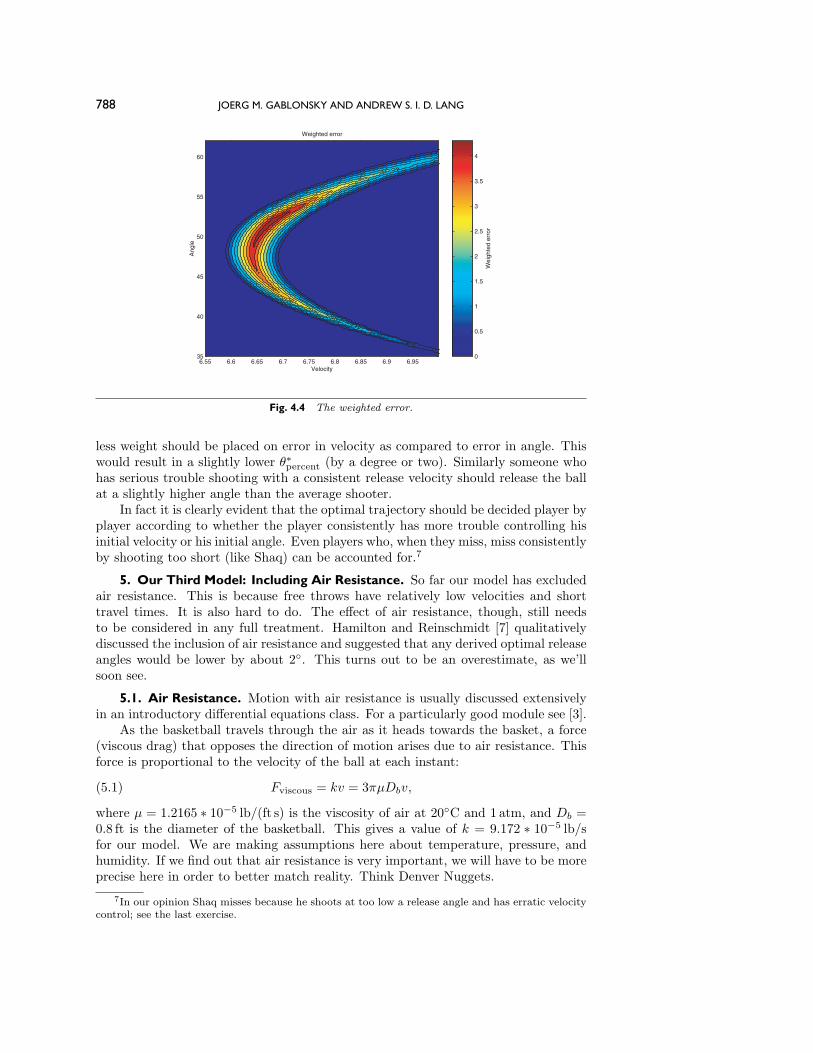
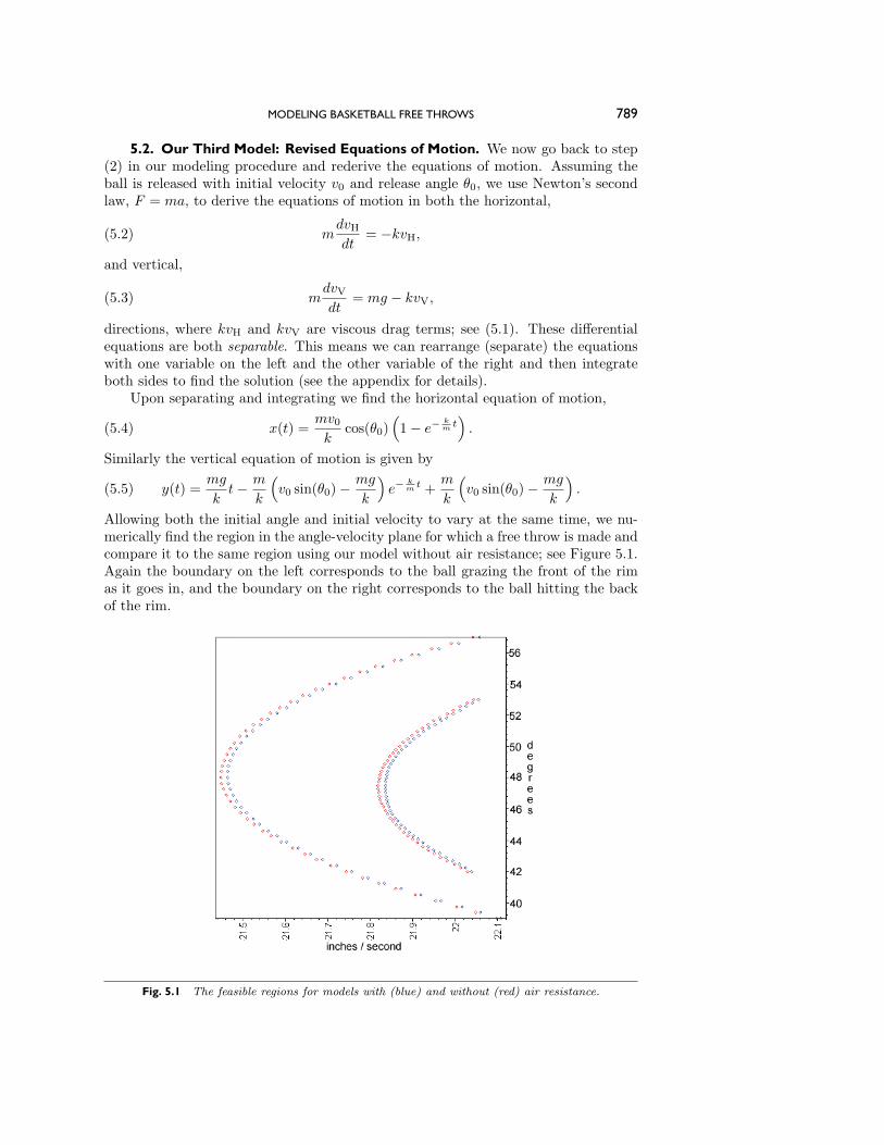
Allowing both the initial angle and initial velocity to vary at the same time, we nu-merically find the region in the angle-velocity plane for which a free throw is made andcompare it to the same region using our model without air resistance; see Figure 5.1.Again the boundary on the left corresponds to the ball grazing the front of the rimas it goes in, and the boundary on the right corresponds to the ball hitting the backof the rim.
Fig. 5.1 The feasible regions for models with (blue) and without (red) air resistance.
790 JOERG M. GABLONSKY AND ANDREW S. I. D. LANG
5.3. Interpreting the Model. As we can clearly see from Figure 5.1, air resis-tance plays a very small part in the trajectory of a free throw. Specifically, includ-ing air resistance increases the optimal trajectory’s initial velocity by approximately0.0381 cm/s for our 7’1” player.
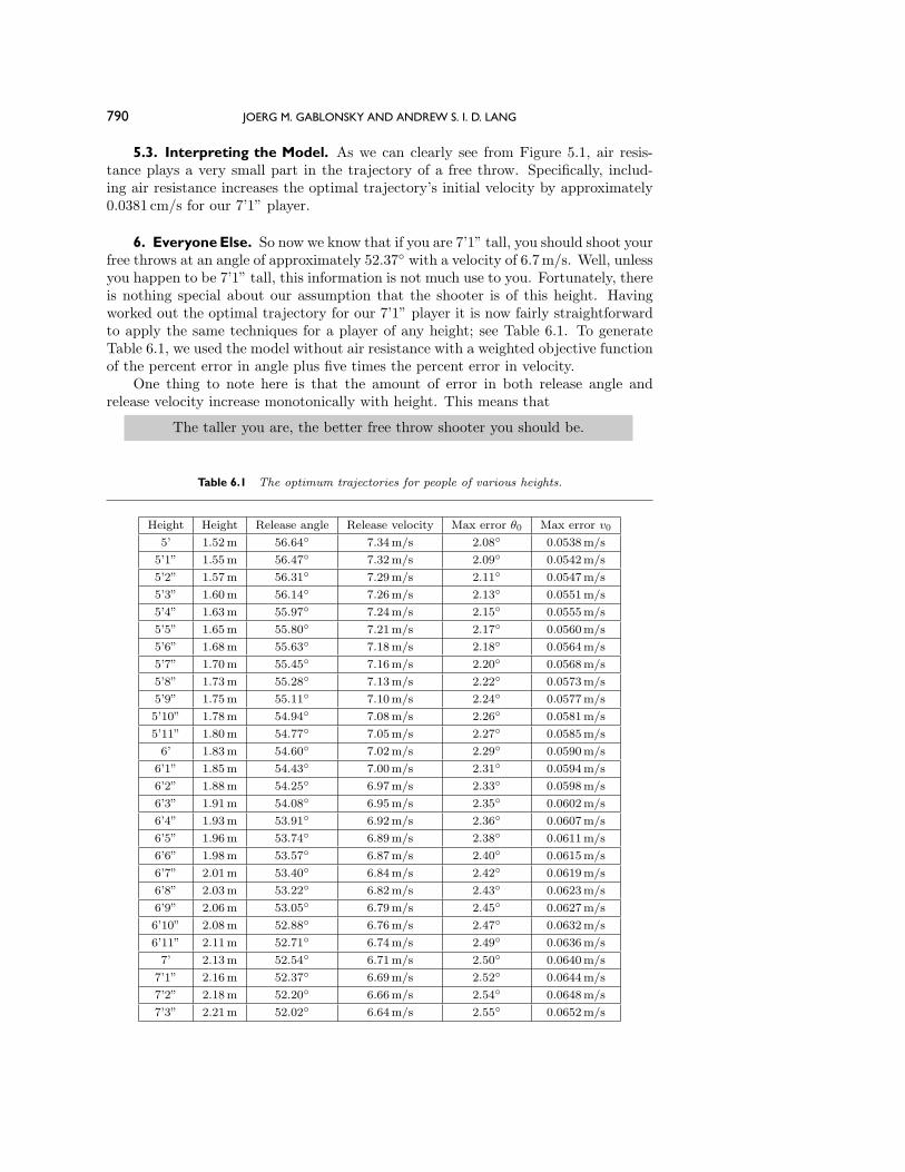
6. EveryoneElse. So now we know that if you are 7’1” tall, you should shoot yourfree throws at an angle of approximately 52.37◦ with a velocity of 6.7 m/s. Well, unlessyou happen to be 7’1” tall, this information is not much use to you. Fortunately, thereis nothing special about our assumption that the shooter is of this height. Havingworked out the optimal trajectory for our 7’1” player it is now fairly straightforwardto apply the same techniques for a player of any height; see Table 6.1. To generateTable 6.1, we used the model without air resistance with a weighted objective functionof the percent error in angle plus five times the percent error in velocity.
One thing to note here is that the amount of error in both release angle andrelease velocity increase monotonically with height. This means that
The taller you are, the better free throw shooter you should be.
Table 6.1 The optimum trajectories for people of various heights.
Height Height Release angle Release velocity Max error θ0 Max error v0
5’ 1.52m 56.64◦ 7.34m/s 2.08◦ 0.0538m/s5’1” 1.55m 56.47◦ 7.32m/s 2.09◦ 0.0542m/s5’2” 1.57m 56.31◦ 7.29m/s 2.11◦ 0.0547m/s5’3” 1.60m 56.14◦ 7.26m/s 2.13◦ 0.0551m/s5’4” 1.63m 55.97◦ 7.24m/s 2.15◦ 0.0555m/s5’5” 1.65m 55.80◦ 7.21m/s 2.17◦ 0.0560m/s5’6” 1.68m 55.63◦ 7.18m/s 2.18◦ 0.0564m/s5’7” 1.70m 55.45◦ 7.16m/s 2.20◦ 0.0568m/s5’8” 1.73m 55.28◦ 7.13m/s 2.22◦ 0.0573m/s5’9” 1.75m 55.11◦ 7.10m/s 2.24◦ 0.0577m/s5’10” 1.78m 54.94◦ 7.08m/s 2.26◦ 0.0581m/s5’11” 1.80m 54.77◦ 7.05m/s 2.27◦ 0.0585m/s6’ 1.83m 54.60◦ 7.02m/s 2.29◦ 0.0590m/s6’1” 1.85m 54.43◦ 7.00m/s 2.31◦ 0.0594m/s6’2” 1.88m 54.25◦ 6.97m/s 2.33◦ 0.0598m/s6’3” 1.91m 54.08◦ 6.95m/s 2.35◦ 0.0602m/s6’4” 1.93m 53.91◦ 6.92m/s 2.36◦ 0.0607m/s6’5” 1.96m 53.74◦ 6.89m/s 2.38◦ 0.0611m/s6’6” 1.98m 53.57◦ 6.87m/s 2.40◦ 0.0615m/s6’7” 2.01m 53.40◦ 6.84m/s 2.42◦ 0.0619m/s6’8” 2.03m 53.22◦ 6.82m/s 2.43◦ 0.0623m/s6’9” 2.06m 53.05◦ 6.79m/s 2.45◦ 0.0627m/s6’10” 2.08m 52.88◦ 6.76m/s 2.47◦ 0.0632m/s6’11” 2.11m 52.71◦ 6.74m/s 2.49◦ 0.0636m/s7’ 2.13m 52.54◦ 6.71m/s 2.50◦ 0.0640m/s7’1” 2.16m 52.37◦ 6.69m/s 2.52◦ 0.0644m/s7’2” 2.18m 52.20◦ 6.66m/s 2.54◦ 0.0648m/s7’3” 2.21m 52.02◦ 6.64m/s 2.55◦ 0.0652m/s
MODELING BASKETBALL FREE THROWS 791
7.2 7.4 7.6 7.8 8 8.2 8.4 8.6 8.8 930
35
40
45
50
55
60
65Height 5.1
Velocity
Ang
le
FrontCenterBackSolution
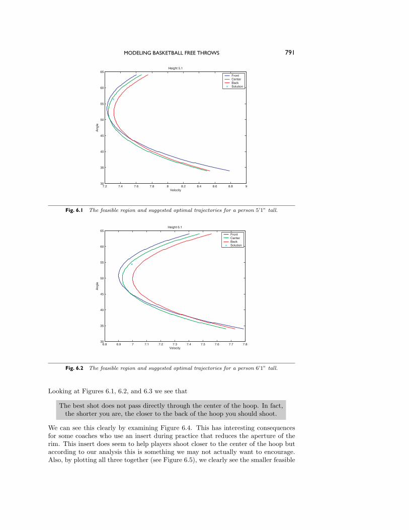
Fig. 6.1 The feasible region and suggested optimal trajectories for a person 5’1” tall.
6.8 6.9 7 7.1 7.2 7.3 7.4 7.5 7.6 7.7 7.830
35
40
45
50
55
60
65Height 6.1
Velocity
Ang
le
FrontCenterBackSolution
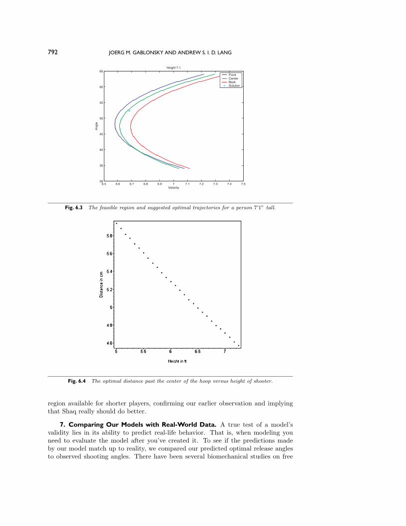
Fig. 6.2 The feasible region and suggested optimal trajectories for a person 6’1” tall.
Looking at Figures 6.1, 6.2, and 6.3 we see that
The best shot does not pass directly through the center of the hoop. In fact,the shorter you are, the closer to the back of the hoop you should shoot.
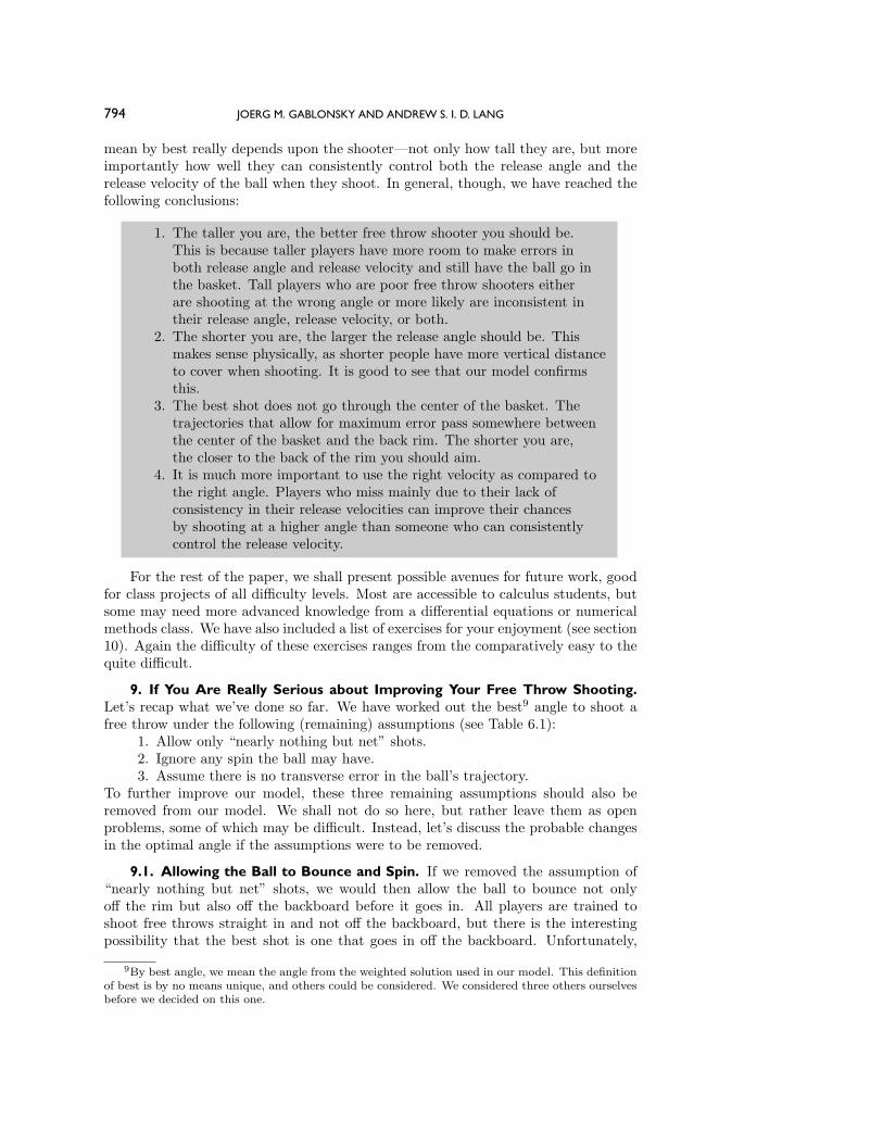
We can see this clearly by examining Figure 6.4. This has interesting consequencesfor some coaches who use an insert during practice that reduces the aperture of therim. This insert does seem to help players shoot closer to the center of the hoop butaccording to our analysis this is something we may not actually want to encourage.Also, by plotting all three together (see Figure 6.5), we clearly see the smaller feasible
792 JOERG M. GABLONSKY AND ANDREW S. I. D. LANG
6.5 6.6 6.7 6.8 6.9 7 7.1 7.2 7.3 7.4 7.530
35
40
45
50
55
60
65Height 7.1
Velocity
Ang
le
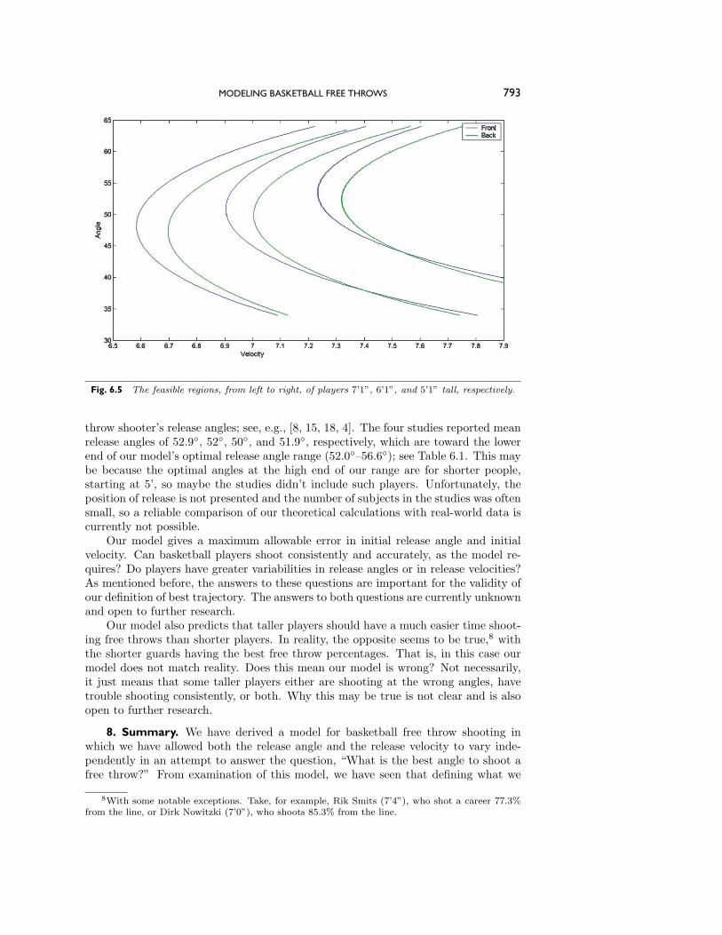
FrontCenterBackSolution
Fig. 6.3 The feasible region and suggested optimal trajectories for a person 7’1” tall.
Fig. 6.4 The optimal distance past the center of the hoop versus height of shooter.
region available for shorter players, confirming our earlier observation and implyingthat Shaq really should do better.
7. Comparing Our Models with Real-World Data. A true test of a model’svalidity lies in its ability to predict real-life behavior. That is, when modeling youneed to evaluate the model after you’ve created it. To see if the predictions madeby our model match up to reality, we compared our predicted optimal release anglesto observed shooting angles. There have been several biomechanical studies on free
MODELING BASKETBALL FREE THROWS 793
Fig. 6.5 The feasible regions, from left to right, of players 7’1”, 6’1”, and 5’1” tall, respectively.
throw shooter’s release angles; see, e.g., [8, 15, 18, 4]. The four studies reported meanrelease angles of 52.9◦, 52◦, 50◦, and 51.9◦, respectively, which are toward the lowerend of our model’s optimal release angle range (52.0◦–56.6◦); see Table 6.1. This maybe because the optimal angles at the high end of our range are for shorter people,starting at 5’, so maybe the studies didn’t include such players. Unfortunately, theposition of release is not presented and the number of subjects in the studies was oftensmall, so a reliable comparison of our theoretical calculations with real-world data iscurrently not possible.
Our model gives a maximum allowable error in initial release angle and initialvelocity. Can basketball players shoot consistently and accurately, as the model re-quires? Do players have greater variabilities in release angles or in release velocities?As mentioned before, the answers to these questions are important for the validity ofour definition of best trajectory. The answers to both questions are currently unknownand open to further research.
Our model also predicts that taller players should have a much easier time shoot-ing free throws than shorter players. In reality, the opposite seems to be true,8 withthe shorter guards having the best free throw percentages. That is, in this case ourmodel does not match reality. Does this mean our model is wrong? Not necessarily,it just means that some taller players either are shooting at the wrong angles, havetrouble shooting consistently, or both. Why this may be true is not clear and is alsoopen to further research.
8. Summary. We have derived a model for basketball free throw shooting inwhich we have allowed both the release angle and the release velocity to vary inde-pendently in an attempt to answer the question, “What is the best angle to shoot afree throw?” From examination of this model, we have seen that defining what we
8With some notable exceptions. Take, for example, Rik Smits (7’4”), who shot a career 77.3%from the line, or Dirk Nowitzki (7’0”), who shoots 85.3% from the line.
794 JOERG M. GABLONSKY AND ANDREW S. I. D. LANG
mean by best really depends upon the shooter—not only how tall they are, but moreimportantly how well they can consistently control both the release angle and therelease velocity of the ball when they shoot. In general, though, we have reached thefollowing conclusions:
1. The taller you are, the better free throw shooter you should be.This is because taller players have more room to make errors inboth release angle and release velocity and still have the ball go inthe basket. Tall players who are poor free throw shooters eitherare shooting at the wrong angle or more likely are inconsistent intheir release angle, release velocity, or both.
2. The shorter you are, the larger the release angle should be. Thismakes sense physically, as shorter people have more vertical distanceto cover when shooting. It is good to see that our model confirmsthis.
3. The best shot does not go through the center of the basket. Thetrajectories that allow for maximum error pass somewhere betweenthe center of the basket and the back rim. The shorter you are,the closer to the back of the rim you should aim.
4. It is much more important to use the right velocity as compared tothe right angle. Players who miss mainly due to their lack ofconsistency in their release velocities can improve their chancesby shooting at a higher angle than someone who can consistentlycontrol the release velocity.
For the rest of the paper, we shall present possible avenues for future work, goodfor class projects of all difficulty levels. Most are accessible to calculus students, butsome may need more advanced knowledge from a differential equations or numericalmethods class. We have also included a list of exercises for your enjoyment (see section10). Again the difficulty of these exercises ranges from the comparatively easy to thequite difficult.
9. If You Are Really Serious about Improving Your Free Throw Shooting.Let’s recap what we’ve done so far. We have worked out the best9 angle to shoot afree throw under the following (remaining) assumptions (see Table 6.1):
1. Allow only “nearly nothing but net” shots.2. Ignore any spin the ball may have.3. Assume there is no transverse error in the ball’s trajectory.
To further improve our model, these three remaining assumptions should also beremoved from our model. We shall not do so here, but rather leave them as openproblems, some of which may be difficult. Instead, let’s discuss the probable changesin the optimal angle if the assumptions were to be removed.
9.1. Allowing the Ball to Bounce and Spin. If we removed the assumption of“nearly nothing but net” shots, we would then allow the ball to bounce not onlyoff the rim but also off the backboard before it goes in. All players are trained toshoot free throws straight in and not off the backboard, but there is the interestingpossibility that the best shot is one that goes in off the backboard. Unfortunately,
9By best angle, we mean the angle from the weighted solution used in our model. This definitionof best is by no means unique, and others could be considered. We considered three others ourselvesbefore we decided on this one.
MODELING BASKETBALL FREE THROWS 795
the model would become significantly more complicated if this assumption were to beremoved.
The way the ball bounces depends on something called the coefficient of restitutionof the ball. This is a measure of how “bouncy” the ball is. An official ball droppedfrom a height of 1.8m (measured from the bottom of the ball) must return to a heightof 1.2–1.4m (measured from the top of the ball); see [13]. This is rather a big rangeof “bounciness,” which would need careful consideration in any new model.
Other things to consider when letting the ball bounce are the softness (or stiffness)of the rim and the spin of the ball. In particular, the optimal trajectory would nowbe one with optimal release angle, release velocity, and release spin, and in reality, aplayer does have to concentrate on all three of these variables when shooting a freethrow. With all these considerations in mind, it is unlikely that the best shot is onewhere you aim to bounce the ball off something before having it go in. Even so, someserious researchers, based upon qualitative investigations, have suggested the optimaltrajectory is a backboard shot; see, e.g., [16].
What does need to be included in any new model (at least as a first step) aretrajectories for which the ball hits the backboard and then either (a) goes directlydown and in or (b) goes in after hitting the front of the rim. For these trajectoriesspin is important. Shooting the ball with backspin should broaden the allowed errorrange e(θ0), though this really needs to be investigated quantitatively.
9.2. Including a Sideways Error. Assuming that there is no transverse error inthe trajectory seems to us to make good sense. Shooting straight is the first thingyou should try to get right when shooting free throws, especially if you want to bea professional. It would be interesting to find out exactly how allowing transverseerror would affect the optimal release angle. With the inclusion of transverse error, toavoid contact with the rim, the distance between any part of the rim and the centerof the ball must remain greater than the radius of the ball throughout its trajectory.Mathematically this problem becomes very interesting and difficult, but the sameideas apply. Additionally we would also be faced with choosing a new definition ofbest. We would have to deal with two initial angles, vertical and horizontal, as wellas the initial velocity and possibly spin. Challenging, but definitely an area wherefuture research needs to be done.
9.3. The Psychology of Free Throw Shooting. We conclude by discussing somenonmathematical considerations for improving basketball free throw shooting.10
Sport psychology has become a serious business. Scores of scientists are out theretrying to invent techniques that will enhance sport performance. Popular techniquesthat seem to work include mental practice, self-affirmation, stress management, andbiofeedback. For example, take mental practice, known to sport psychologists asvisuo-motor behavior rehearsal. Recent studies [12, 11] claim to show that mentalpractice enhances free throw shooting performance.
Another technique that seems to help free throw shooting is having a preshotroutine [5]. A preshot routine is a set pattern of actions and thoughts performedbefore every free throw. Indeed, many professional basketball players have preshotroutines, some of which are unusual [1]. In short, free throw shooting can be as mucha mental task as a physical one. And I thought I was just a bad shot!
10Are there really areas where mathematics doesn’t apply? Of course not; the mathematics usedto do research in the areas discussed in this section we call statistics.
796 JOERG M. GABLONSKY AND ANDREW S. I. D. LANG
10. Exercises. Here are some problems the reader may wish to consider:1. In our first simplifying assumption we allow only nearly nothing but net shots,
whereby the ball is allowed to hit the back rim, but only if the center of theball is at or below the basket height when it does so. How would you redefine“nearly nothing but net” to allow for all trajectories that hit the back rimand then go in (without hitting the backboard)? Using this new definition of“nearly nothing but net,” would you expect the optimal angle to be higher,lower, or the same as before? Why?
2. Discuss the effect of spin on the definition of “nearly nothing but net.” Seeexercise 1.
3. Use trigonometry to explain Figure 3.3.4. Use (3.7) and (3.8) to derive (3.9).5. Derive (3.10). From your derivation, explain why the ball is moving down,
and not up, as it passes through the hoop.6. Following the beginning of section 3.5, use a computer algebra system to plote(θ0) for someone of your own height. Compare your graph with Figure 3.5.
7. We noted in section 3.5 that for certain (v0, θ0) pairs that result in the bas-ketball passing through the center of the hoop, changing the release angle θ0(but keeping v0 fixed) will never cause the ball to hit the back rim. Locateand describe the region where this happens in Figure 4.1. Physically what ishappening here?
8. Use numerical methods to construct your own feasible regions for Shaq andfor yourself, i.e., for someone of your height. Use numerical integration orsome other technique to approximate the areas of the two regions. Are theydifferent? What can you conclude?
9. In section 4.2, we claim that it is “obvious” that it is more important to usethe right velocity as compared to the right angle. Give details explaining whyour claim makes sense for our model?
10. Derive (5.5) by using the technique of separation of variables to solve (5.3).Hint: Look in the appendix.
11. In Figures 6.1–6.3, the feasible regions for players 5’1”, 6’1”, and 7’1” tall, theleft and right boundaries intersect. Estimate the location where this occursfor Shaq. What does this correspond to physically?
12. At the end of section 7, we mentioned that some taller players have poor freethrow shooting percentages. Make several conjectures about why this maybe true. How would you test your conjectures?
13. From a purely mathematical point of view it is interesting to imagine the ballbeing a shape other than round. Spin now becomes important. Why?
14. Suppose you have been hired by Shaq to help him with his free throws. Dis-cuss in detail how you would accomplish this.
Appendix. Separation of Variables. Separation of variables is a mathemati-cal technique used to solve first order separable differential equations. A first orderdifferential equation can be written in the form
dy
dx= f(x, y).(A.1)
If the function f(x, y) can be written as f(x, y) = g(x)h(y), the equation is calledseparable and can be solved using separation of variables. If your equation is notseparable, you have to use more powerful techniques to solve it. These techniques are
MODELING BASKETBALL FREE THROWS 797
discussed in a standard differential equations course. Assuming that our equation isseparable, we solve it as follows:
1. Separate. Rewrite the equation as
dy
dx= g(x)h(y)(A.2)
and separate (move all the x’s on one side and all the y’s on the other side),to obtain
1h(y)
dy = g(x)dx.(A.3)
2. Integrate. Now that we have just one variable on each side, we can integrate(antidifferentiate) both sides to obtain a solution:
∫1
h(y)dy =
∫g(x)dx.(A.4)
A.1. Example. We shall use separation of variables to solve (5.2), the first dif-ferential equation of the air resistance section. We’ll leave the solution of the otherdifferential equation as an exercise. Recall the differential equation for the horizontalmotion:
mdvh
dt= −kvh,(A.5)
where m and k are constants. Separating, we obtain
1vhdvh = − k
mdt.(A.6)
Integrating both sides,∫
1vhdvh = − k
m
∫1dt,(A.7)
we obtain
ln vh = − kmt+ c,(A.8)
where c is the constant of integration. Exponentiating both side to remove the loga-rithm, and using the initial condition vh(0) = v0 cos (θ0) to find c, we obtain
vh =dx
dt= v0 cos (θ0) e−
km t.(A.9)
This equation, in x and t, is also separable. Separating, we obtain
dx = v0 cos (θ0) e−km tdt.(A.10)
Integrating both sides,∫
1dx = v0 cos (θ0)∫e−
km tdt,(A.11)
798 JOERG M. GABLONSKY AND ANDREW S. I. D. LANG
we obtain
x = −mv0
kcos (θ0) e−
km t + c,(A.12)
where c is again a constant of integration. Using the initial condition x(0) = 0 to findc, we obtain (cf. (5.4))
x(t) =mv0
kcos(θ0)
(1− e− k
m t).(A.13)
Acknowledgment. The authors thank Yves Nievergelt and John Lewis for theirmany helpful suggestions.
REFERENCES
[1] M. Bamberger, Everything you always wanted to know about free throws, Sports Illustrated,88 (1998), pp. 15–21.
[2] P. Brancazio, Physics of basketball, Amer. J. Phys., 49 (1981), pp. 356–365.[3] H. E. Donley, The drag force on a sphere, UMAP J., 12 (1991), pp. 47–80.[4] M. R. Eddings, Effect of Manipulating Angle of Projection on Height of Release and Accuracy
in the Basketball Free Throw: A Biomechanical Study, Master’s thesis, California StateUniversity, 1996.
[5] W. F. Gayton, K. L. Cielinski, W. J. Francis-Kensington, and J. F. Hearns, Effects ofpreshot routine on free-throw shooting, Perceptual and Motor Skills, 68 (1989), pp. 317–318.
[6] D. Halladay, R. Resnick, and J. Walker, Fundamentals of Physics, John Wiley & Sons,New York, 1997.
[7] G. R. Hamilton and C. Reinschmidt, Optimal trajectory for the basketball free throw, J.Sports Sci., 15 (1997), pp. 491–504.
[8] J. Hudson, A biomechanical analysis by skill level of free throw shooting in basketball, inBiomechanics in Sports, Academic Publishers, Del Mar, CA, 1982, pp. 95–102.
[9] D. Indraneel and J. E. Dennis, Normal-Boundary Intersection (NBI), is a new technique forsolving nonlinear multicriteria optimization problems., SIAM J. Optim., 8 (1998), pp. 631–657.
[10] C. T. Kelley, Iterative Methods for Optimization, Frontiers Appl. Math. 18, SIAM, Philadel-phia, 1999.
[11] B. J. Kolonay, Visual Motor Behavior Rehearsal, or VMBR, Master’s thesis, Hunter College,New York, 1977.
[12] D. M. Onestak, The effects of progressive relaxation, mental practice, and hypnosis on athleticperformance, J. Sports Behav., 14 (1997), pp. 247–282.
[13] T. Pocock, Official Rules of Sports & Games, Kingswood Press, 1992.[14] P. C. Reddy, Physics of Sports (Basketball), Ashish Publishing House, New Delhi, India, 1992.[15] M. N. Satern, Comparison of adult male and female performance on the basketball free throw
to that of adolescent boys, Biomech. Sports, 6 (1988), pp. 465–468.[16] K. Shibukawa, Velocity conditions of basketball shooting, Bull. Instit. Sport Sci., 13 (1975),
pp. 59–64.[17] G. Thomas and R. Finney, Calculus and Analytic Geometry, Addison-Wesley, Reading, MA,
1996.[18] E. Tsarouchas, K. Kalamaras, A. Giavroglou, and S. Prassas, Biomechanical analysis
of free throw shooting in basketball, Biomech. Sports, 6 (1988), pp. 551–560.[19] R. E. Vaughn and B. Kozar, Intra-individual variability for basketball free throws, Biomech.
Sports, 11 (1993), pp. 305–308.