Modeling the Macroeconomic Effects of a Universal...

Modeling the Macroeconomic

Effects of a Universal Basic

Income

Report by Michalis Nikiforos, Marshall Steinbaum, and Gennaro Zezza

AUGUST 2017

2 CREATIVE COMMONS COPYRIGHT 2017 | ROOSEVELTINSTITUTE .ORG

Acknowledgments The authors are grateful to Narayana Kocherlakota for his feedback and comments. Roosevelt staff Nell Abernathy,

Rakeen Mabud, Marybeth Seitz-Brown, Alex Tucciarone, and Devin Duffy provided help throughout the project. The

Roosevelt Institute is grateful to the Economic Security Project, the Nathan Cummings Foundation, and the Joyce

Foundation for their support.

About the Authors

Michalis Nikiforos is a Levy Institute research scholar working in the State of the US and World Economies

program. He works on the Institute’s stock-flow consistent macroeconomic model for the US economy and

contributed to the recent construction of a similar model for Greece. He has coauthored several policy reports

on the prospects of the US and European economies. His research interests include macroeconomic theory

and policy, distribution of income, the theory of economic fluctuations, political economy, and economics of

monetary union. He has published several papers in peer-reviewed journals, while various other papers have

appeared in the Levy Economics Institute Working Paper Series. Nikiforos holds a BA in economics and an

M.Sc. in economic theory from the Athens University of Economics and Business, and an M.Phil. and a

Ph.D. in economics from The New School for Social Research.

Marshall Steinbaum is Research Director and Fellow at the Roosevelt Institute, where he researches

inequality, tax policy, the (poor) functioning of the labor market, antitrust and competition policy, and

student debt and higher education policy. He is an editor of the forthcoming After Piketty: the Agenda for

Economics and Inequality (Harvard University Press, 2017), and his work has appeared in the Industrial and

Labor Relations Review, Democracy, Boston Review, American Prospect, and The New Republic.

Gennaro Zezza is Associate Professor in Economics at Dipartimento di Economia e Giurisprudenza,

Università di Cassino e del Lazio meridionale, Italy, and Research Scholar at the Levy Economics Institute

of Bard College, US. His main area of research is in post-Keynesian stock-flow-consistent modeling: he

helped develop this approach working with the late Wynne Godley in the United Kingdom, Denmark, as

well as at the Levy Institute. He contributed to most Levy Institute Strategic Analysis of the U.S. economy

and Greece. In 2016 he worked with FAO on models for long-term projections, and with the government of

Ecuador for developing a model for policy analysis. His most recent publication is ‘Stock-flow-consistent

macroeconomic models: A survey’ (joint with M.Nikiforos), forthcoming in Journal of Economic Surveys.

About the Roosevelt Institute

Until economic and social rules work for all, they’re not working. Inspired by the legacy of Franklin and

Eleanor, the Roosevelt Institute reimagines America as it should be: a place where hard work is rewarded,

everyone participates, and everyone enjoys a fair share of our collective prosperity. We believe that when

the rules work against this vision, it’s our responsibility to recreate them.

We bring together thousands of thinkers and doers—from a new generation of leaders in every state to Nobel

laureate economists—working to redefine the rules that guide our social and economic realities. We rethink

and reshape everything from local policy to federal legislation, orienting toward a new economic and

political system: one built by many for the good of all.


Executive Summary

How would a massive federal spending program like a universal basic income (UBI) affect the

macroeconomy? We use the Levy Institute macroeconometric model to estimate the impact of three versions of

such an unconditional cash assistance program over an eight-year time horizon. Overall, we find that the

economy can not only withstand large increases in federal spending, but could also grow thanks to the

stimulative effects of cash transfers on the economy.

We examine three versions of unconditional cash transfers: $1,000 a month to all adults, $500 a month to all

adults, and a $250 a month child allowance. For each of the three versions, we model the macroeconomic

effects of these transfers using two different financing plans - increasing the federal debt, or fully funding the

increased spending with increased taxes on households - and compare the effects to the Levy model’s baseline

growth rate forecast. Our findings include the following:

For all three designs, enacting a UBI and paying for it by increasing the federal debt would grow the

economy. Under the smallest spending scenario, $250 per month for each child, GDP is 0.79% larger

than under the baseline forecast after eight years. According to the Levy Model, the largest cash

program - $1,000 for all adults annually - expands the economy by 12.56% over the baseline after eight

years. After eight years of enactment, the stimulative effects of the program dissipate and GDP growth

returns to the baseline forecast, but the level of output remains permanently higher.

When paying for the policy by increasing taxes on households, the Levy model forecasts no effect on the

economy. In effect, it gives to households with one hand what it is takes away with the other.

However, when the model is adapted to include distributional effects, the economy grows, even in the

tax-financed scenarios. This occurs because the distributional model incorporates the idea that an extra

dollar in the hands of lower income households leads to higher spending. In other words, the

households that pay more in taxes than they receive in cash assistance have a low propensity to

consume, and those that receive more in assistance than they pay in taxes have a high propensity to

consume. Thus, even when the policy is tax- rather than debt-financed, there is an increase in output,

employment, prices, and wages.

Levy’s Keynesian model incorporates a series of assumptions based on rigorous empirical studies of the micro

and macro effects of unconditional cash transfers, taxation and government net spending and borrowing (see

Marinescu (2017), Mason (2017), Coibion et al (2017), and Konczal and Steinbaum (2016)). Fundamentally,

the larger the size of the UBI, the larger the increase in aggregate demand and thus the larger the resulting

economy is. The individual macroeconomic indicators are (qualitatively) what one would predict given an

increase in aggregate demand: in addition to the increase in output, employment, labor force participation,

prices, and wages all go up as well. Even in a deficit-financed policy, an increase in the government’s

liabilities is mitigated by the increase in aggregate demand.

Specifically, the Levy model assumes that the economy is not currently operating near potential output (Mason

2017) and makes two related microeconomic assumptions: (1) unconditional cash transfers do not reduce

household labor supply; and (2) increasing government revenue by increasing taxes levied on households does

not change household behavior. Other macroeconomic models would make different, likely less optimistic

forecasts, because they would disagree with these assumptions.

Estimating the macroeconomic effects of UBI is a critical component of any policy evaluation, because what

would appear to be a zero-sum transfer in static terms (money is simply transferred from some households to

others) turns out to be positive sum in the macro simulation, thanks to the increase in aggregate demand and

therefore in the size of the economy.


Introduction

A policy of universal, unconditional cash assistance (Universal Basic Income, or “UBI” in general terms)

would substantially alleviate extreme poverty, which has been on the rise during an era in which existing

unconditional transfer policies have been scaled back and repurposed, while the labor market is proving less

reliable as a source of support than it once was, especially for low-wage workers.i But what would the impact

of such a policy be on the macroeconomy?

To answer that question, we used the Levy Institute Macro-Econometric Model to estimate the impact of three

versions of unconditional cash assistance over an eight-year horizon. The Levy Institute model is particularly

well suited to answer this question, because of the emphasis it places on household balance sheets as a driver

of macroeconomic outcomes. The whole aim of the policy is to render households more financially secure,

therefore a model that incorporates the financial security of households into macroeconomic outcomes is

critical to answering the question about how a UBI would affect the macroeconomy.

The Levy Institute has been constructing and updating its model for many years in order to provide factual

predictions about the macroeconomy by comparing its forecasts with realized outcomes. The approach taken in

this paper uses the Levy model to forecast the macroeconomy eight years into the future, holding current

policies constant. This is the “baseline” forecast, for our purposes. We then perform a series of policy

counterfactuals related to enacting a UBI of different sizes and target populations, and compare the eight-year

prediction for the macroeconomy given the policy counterfactuals to the baseline forecast. We report the

difference in key macroeconomic and labor market indicators between these counterfactuals and the baseline

as the “effect” of UBI.

The Levy model is a purely macro model: it contains aggregate economic actors and treats them as individuals.

For example, the “household sector” is one large household, the “corporate sector” is one large firm, and the

“government” is one unitary organization that conducts both fiscal and monetary policy. This is standard in the

macroeconomics literature but is not necessarily well suited to study the effect of a UBI on the macroeconomy,

because a UBI inherently affects the distribution of income among households. If the distribution of income

matters for macroeconomic outcomes—and there is reason to think that it does—then a policy like UBI that

alters the distribution of income among households needs to be interpreted in light of a distributional model in

order to forecast its macroeconomic effect. We thus modify the basic model with adjustments for heterogeneity

in income taxes paid and in propensity to consume across households, both of which (we show) are relevant to

forecasting the macroeconomic impact of UBI.

Our results are very clear: enacting a UBI and paying for it by increasing the federal debt would be

expansionary, because it would increase aggregate demand. When the policy is first enacted, economic growth

is higher than in the baseline as the economy converges to a larger size. Within eight years of enactment,

growth returns to the same rate as in the baseline, with output at a permanently higher level.

The larger the size of the UBI, the larger the increase in aggregate demand and thus the larger the resulting

economy is. The individual macroeconomic indicators are (qualitatively) what one would predict given an

increase in aggregate demand: in addition to the increase in output, employment, labor force participation,

prices, and wages all go up, as well. Since the policy is deficit financed, it increases the government’s

liabilities, but because of the stimulative effect of the policy, that increase in debt is less than it would be if the

policy did not increase aggregate demand.

i There is a large literature on these trends. See Edin and Shaefer (2015) and Rogers (2017) for excellent introductions.


When paying for the policy by increasing taxes on households rather than paying for the policy with debt, the

policy is not expansionary. In effect, it is giving to households with one hand what it is taking away with the

other. There is no net effect.

When distributional implications are taken into account, the stimulative effect of the policy increases, because

households that gain on net have a high propensity to consume relative to those that lose. Thus, even when the

policy is tax- rather than debt-financed, there is an increase in output, employment, prices, and wages, because

the households that pay more in taxes than they receive in cash assistance have a low propensity to consume,

and those that receive more in assistance than they pay in taxes have a high propensity to consume. This

exercise shows that estimating the macroeconomic impact of UBI is a critical component of any policy

evaluation, because what would appear to be a zero-sum transfer in static terms (money is simply transferred

from some households to others) turns out to be positive sum in the macro simulation due to the increase in

aggregate demand and therefore in the size of the economy.

There are, of course, many macroeconomic models to use, and one that emphasizes the financial status of

households, as Levy’s does, will unavoidably discount other factors. The factor that other models emphasize

which is not present in the Levy Model is “potential output”—that the size of the macroeconomy is

theoretically limited by supply constraints, and that once these bind, the effect of further expansion in

aggregate demand is primarily to increase inflation. We judge that the economy has been operating below

potential for a long time now, certainly since the beginning of the financial crisis in 2007 and arguably even

before that. There is an active debate over whether that underperformance has in turn caused a decline in the

level of potential output, such that an attempt to achieve the level of potential output predicted for 2017–2020

pre-recession would create inflation before the economy reached that level. Given the apparent absence of

inflationary pressures to date and other evidence that the economy is not supply-constrained, we take the view

that it would not, or at least that there is no empirical evidence that it would.ii Other macroeconomic models

would disagree.

There are two crucial and immediately relevant microeconomic assumptions underlying the more general

contention that the economy is not currently operating near potential output. Those micro assumptions are:

1. Unconditional cash transfers do not reduce household labor supply.

2. Increasing government revenue by increasing taxes levied on households does not change household

behavior.

In the discussion below, we motivate these assumptions in the empirical literature on micro and macro effects

of unconditional cash transfers, taxation, and government net spending and borrowing.

This paper is organized as follows: Section 2 gives a brief overview of the Levy Macro-Econometric model,

and section 3 explains how it works. Section 4 discusses how we add a distributional element to the underlying

aggregate model. Section 5 presents the alternative unconditional cash scenarios. Section 6 explains how the

policy is implemented over time within the model. Section 7 presents the results, and section 8 concludes with

a discussion of their significance and context.

ii See Mason (2017) and Coibion et al (2017) for a discussion of whether potential output responds to cyclical fluctuations in

aggregate demand. See Konczal and Steinbaum (2016) for evidence that the labor market is underperforming thanks to a “structural”

lack of demand.


2. The Levy Macro-Economic Model

The Levy Macro-Economic model is used to examine the medium-run prospects of the U.S. economy and to

simulate the effects of alternative policy options. It is Keynesian because the macroeconomic performance of

the economy is driven by aggregate demand both in the short- and medium-run. Moreover, it follows the so-

called Stock-Flow Consistent macroeconomic methodology, which allows for an integrated treatment of the

real and financial sides of the economy; factors that do not have any role in more conventional applied macro

models, like household or corporate sector debt, take center stage in our analysis.iii By contrast, the Levy

model contains no aggregate production function, so it has no way of decomposing the causes of macro

dynamics into the effect of increased factor utilization versus the effect of increased factor productivity.

The model was created in the late 1990s by Wynne Godley and was used in subsequent years to argue that the

U.S. economy was on an unsustainable path and that crisis was imminent due to the increasing indebtedness of

the private sector (Godley 1999). A relatively recent description of the Levy model can be found in Zezza

(2009).

In the last few years—after the crisis of 2007–09—analyses based on the Levy model have argued that

conventional projections for the U.S. economy (for example, those produced by the CBO or the IMF) have

consistently been overoptimistic. Based on the model simulations, the strong rebound in economic growth that

these projections were envisioning would require another round of increasing indebtedness on behalf of the

private sector, especially for households. Something like this is not plausible, but even if it happened, it would

end the same way it ended in previous crises.iv

The same reports have also demonstrated that the extreme inequality in income distribution was one of the

main causes of the economic crisis, and is now one of the main reasons why the US economy faces the

prospect of secular stagnation. Moreover, they argued in favor of a large public infrastructure program and

have examined the potential impact of a sharp drop in the (currently overvalued) stock market.

3. The structure of the model

The Keynesian nature of the model means that the main driver of economic activity is aggregate demand.

Demand is further decomposed into private expenditure (consumption and investment), government

expenditure, and net exports.

All of these components of demand, except government expenditure, are econometrically estimated. The main

drivers of consumption are the disposable income and the net wealth of the households. Generally, investment

is determined by the level of economic activity. Exports are mainly a function of the GDP of the trading

partners of the U.S., the relative prices between the US economy and its trading partners, and the nominal

exchange rate. Finally, imports are a function of the US GDP, relative prices, and the nominal exchange rate.

The index for the GDP and inflation of the US trading partners is derived using the total trade weights

published by the Federal Reserve Board, and information on each individual country from international or

national databases.v For a discussion of the process, see Dos Santos, Shaikh, and Zezza (2003).

iii For a recent discussion of the Stock-flow consistent approach to macroeconomic analysis see Nikiforos and Zezza (2017). iv Recent analyses of the United States economy based on the Levy model include Papadimitriou, Hannsgen and Nikiforos (2013),

Papadimitriou et al (2014, 2015), Papadimitriou, Nikiforos and Zezza (2016) and Nikiforos and Zezza (2017). v The trade weights of the FRB are available at https://www.federalreserve.gov/releases/h10/Weights/

https://www.federalreserve.gov/releases/h10/Weights/


The behavior of the government is endogenously determined based on the level of economic activity and a

series of (exogenous) policy instruments, related to the various components of government expenditure

(government purchases and transfers) and revenues (tax rates, social security contributions of firms and

households, etc.).

The model also includes a labor market, in which labor force participation and employment rates are a positive

function of the level of economic activity. The nominal wage increases with the level of capacity utilization,

which is pro-cyclical. Finally, the price level is a positive function of the unit labor cost and the price level of

imported goods.

The Levy model is computed as a simultaneous nonlinear system in EViews.

4. Capturing distributional effects

The Levy model is an aggregate model and the household sector is treated as a whole. However, the

introduction of a policy like a universal basic income has important distributional dimensions that need to be

taken into account in our simulations if distribution affects macroeconomic dynamics. In the Levy model, it

does.

For example, among the scenarios we simulate is a fiscally neutral variation of the UBI program. In an

aggregate model, such a program has negligible effects because the increase in the income of the households

(in aggregate) achieved through the introduction of the UBI is fully compensated by the increase in taxation of

households in aggregate. This leaves their disposable income, and therefore the level of economic activity,

unchanged. In reality, however, a program like this—to the extent that it is financed by the increase in the taxes

of households in high-income brackets—implies a more egalitarian distribution of income. From a

macroeconomic point of view, that means income gains for households with a higher propensity to consume

and income losses for households with a lower propensity to consume. Therefore—and to the extent that this

redistribution of income does not have other negative effects on other components of aggregate demand—even

a fiscally neutral UBI has a positive effect on consumption and the level of economic activity.

To evaluate these effects, we supplement our simulations with calculations that take into account the

differential propensities to consume and effective tax rates of households in different income brackets. We use

information from The Distribution of Household Income and Federal Taxes database of the Congressional

Budget Office (CBO 2016) on the distribution of income and the implicit average tax rate by income bracket.

An important piece of information that we need is the marginal propensity to consume of the households in the

various income brackets. The overall marginal propensity to consume produced by the econometric results of

our model is 0.7. However, a casual look at the data (e.g., the Consumer Expenditure Survey of the Bureau of

Labor Statistics [BLS 2017]), alongside careful empirical studies, shows that the propensity to consume is

lower for households at higher income brackets.vi

vi Dynan et al. (2004) estimate the saving rates for households in different income brackets. Carroll et al. (2017) estimate the relation

between wealth distribution and the marginal propensity to consume and provide a review of the recent related literature.


Nevertheless, the estimates in the related literature are not suitable for direct use in our calculations, either

because they have different income brackets or because they refer to the marginal propensity to consume out of

wealth rather than income, or because they refer to consumption of a certain kind of goods (e.g. durables and

non-durables). Moreover, the Consumer Expenditure Survey of the BLS provides information for the average

but not the marginal propensity to consume as a function of income.

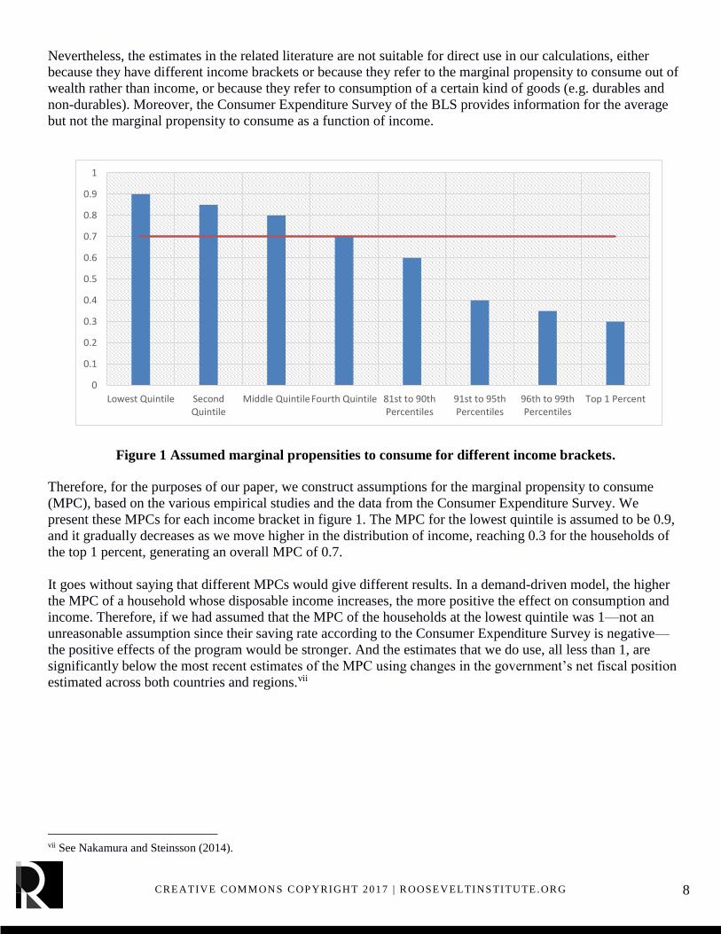
Therefore, for the purposes of our paper, we construct assumptions for the marginal propensity to consume

(MPC), based on the various empirical studies and the data from the Consumer Expenditure Survey. We

present these MPCs for each income bracket in figure 1. The MPC for the lowest quintile is assumed to be 0.9,

and it gradually decreases as we move higher in the distribution of income, reaching 0.3 for the households of

the top 1 percent, generating an overall MPC of 0.7.

It goes without saying that different MPCs would give different results. In a demand-driven model, the higher

the MPC of a household whose disposable income increases, the more positive the effect on consumption and

income. Therefore, if we had assumed that the MPC of the households at the lowest quintile was 1—not an

unreasonable assumption since their saving rate according to the Consumer Expenditure Survey is negative—

the positive effects of the program would be stronger. And the estimates that we do use, all less than 1, are

significantly below the most recent estimates of the MPC using changes in the government’s net fiscal position

estimated across both countries and regions.vii

vii See Nakamura and Steinsson (2014).

0

0.1

0.2

0.3

0.4

0.5

0.6

0.7

0.8

0.9

1

Lowest Quintile SecondQuintile

Middle Quintile Fourth Quintile 81st to 90thPercentiles

91st to 95thPercentiles

96th to 99thPercentiles

Top 1 Percent

Figure 1 Assumed marginal propensities to consume for different income brackets.


5. Three UBI proposals

We will examine three alternative proposals for the introduction of a universal basic income in the United

States, namely:

1. A “child allowance” of $250/month per child under 16

2. A “base” income of $500/month for all adults

3. A “basic” income of $1000/month for all adults

As of July, 2016, the US Census Bureau estimates the total US population to be at 323 million, with the

percentage of persons under 18 years at 22.9 percent.viii We use the civilian non-institutional population 16 and

over from the BLS to obtain the number of children under 16, which is around 69.5 million.ix Proposal 1 would

therefore have an annual cost of $208 billion. The size of this proposal is close to 1% of GDP (it is 1.1% of

GDP) and can therefore also serve as a reference point.

Moreover, the above figures imply that the number of adults involved in policies 2 and 3 will be roughly 249

million, with an annual cost for proposal 2 at $1,495 billion. The cost of proposal 3 would be twice this

amount, around $2,990 billion.

For each of these policies we will consider two alternative options for financing them. First, a pure government

deficit-financing option, where the increase in the government transfers for the UBI leads to an

equiproportional increase in the government’s deficit, save for the change in the spending due to the changes in

the level economy activity caused by the introduction of the program. Second, a fiscally-neutral option, where

the increase in the spending is matched by an ex ante equal increase in the taxes paid by the households.

Moreover, for each of these six scenarios (the three deficit-financed designs and the three fiscally-neutral

designs) we provide a separate simulation that takes into account the distributional effects, as they were

explained in the previous section.x

viii The population statistics of the US Census Bureau can be found at https://www.census.gov/topics/population.html ix The data from the BLS can be found at https://www.bls.gov/lau/rdscnp16.htm x We should note that we do not attempt to model the allocation of the child benefit across households by whether they have children.

If the distribution of children across households differs from the distribution of income across households, which is quite likely

(children are less unequally distributed than income but more unequally distributed than an equal universal transfer), that would have

an effect on the realized macroeconomic impact of a child allowance that is different than the one we forecast here.

https://www.census.gov/topics/population.html

https://www.bls.gov/lau/rdscnp16.htm


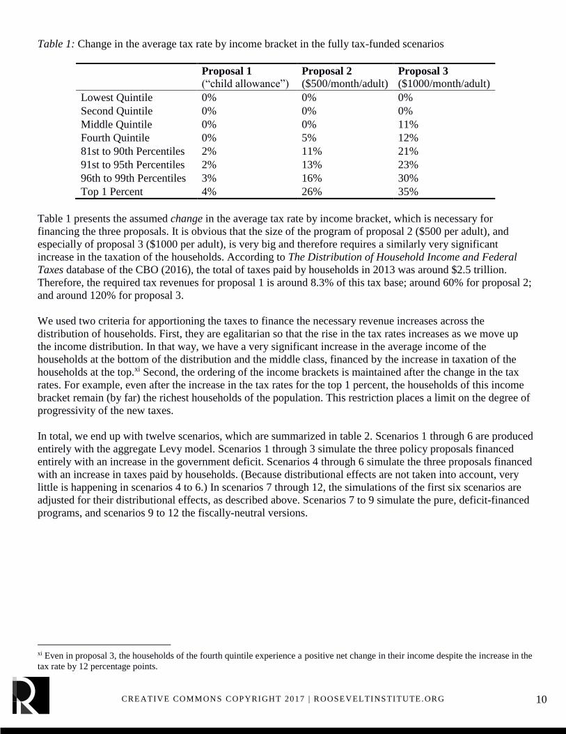
Table 1: Change in the average tax rate by income bracket in the fully tax-funded scenarios

Proposal 1 (“child allowance”)

Proposal 2 ($500/month/adult)


Lowest Quintile 0% 0% 0%

Second Quintile 0% 0% 0%

Middle Quintile 0% 0% 11%

Fourth Quintile 0% 5% 12%

81st to 90th Percentiles 2% 11% 21%

91st to 95th Percentiles 2% 13% 23%

96th to 99th Percentiles 3% 16% 30%

Top 1 Percent 4% 26% 35%

Table 1 presents the assumed change in the average tax rate by income bracket, which is necessary for

financing the three proposals. It is obvious that the size of the program of proposal 2 ($500 per adult), and

especially of proposal 3 ($1000 per adult), is very big and therefore requires a similarly very significant

increase in the taxation of the households. According to The Distribution of Household Income and Federal

Taxes database of the CBO (2016), the total of taxes paid by households in 2013 was around $2.5 trillion.

Therefore, the required tax revenues for proposal 1 is around 8.3% of this tax base; around 60% for proposal 2;

and around 120% for proposal 3.

We used two criteria for apportioning the taxes to finance the necessary revenue increases across the

distribution of households. First, they are egalitarian so that the rise in the tax rates increases as we move up

the income distribution. In that way, we have a very significant increase in the average income of the

households at the bottom of the distribution and the middle class, financed by the increase in taxation of the

households at the top.xi Second, the ordering of the income brackets is maintained after the change in the tax

rates. For example, even after the increase in the tax rates for the top 1 percent, the households of this income

bracket remain (by far) the richest households of the population. This restriction places a limit on the degree of

progressivity of the new taxes.

In total, we end up with twelve scenarios, which are summarized in table 2. Scenarios 1 through 6 are produced

entirely with the aggregate Levy model. Scenarios 1 through 3 simulate the three policy proposals financed

entirely with an increase in the government deficit. Scenarios 4 through 6 simulate the three proposals financed

with an increase in taxes paid by households. (Because distributional effects are not taken into account, very

little is happening in scenarios 4 to 6.) In scenarios 7 through 12, the simulations of the first six scenarios are

adjusted for their distributional effects, as described above. Scenarios 7 to 9 simulate the pure, deficit-financed

programs, and scenarios 9 to 12 the fiscally-neutral versions.

xi Even in proposal 3, the households of the fourth quintile experience a positive net change in their income despite the increase in the

tax rate by 12 percentage points.


Table 2: Summary of the 12 simulated scenarios

Deficit

Spending

Fully Tax-

funded

Deficit

Spending

+Distribution

Fully tax-funded

+Distribution

Proposal 1 ("child allowance")

Sc. 1 Sc. 4 Sc. 7 Sc. 10


Sc. 2 Sc. 5 Sc. 8 Sc. 11


Sc. 3 Sc. 6 Sc. 9 Sc. 12

The two sets of scenarios (deficit-financed and fully tax-funded) provide a benchmark. An actual proposal for

unconditional cash income could be funded by some mix of the two, whose effects would lie somewhere in

between the results we report here.

6. Implementation of simulations

In our simulations, we assume that the UBI proposals are gradually implemented over a period of four years,

starting in the first quarter of 2017. Overall, the projection period of the simulations is eight years, 2017 to

2024, which gives enough time for potential lagged effects.

The twelve scenarios are simulated on top of a baseline scenario, which is constructed with reference to the

latest Budget and Economic Outlook of the CBO (2017). The baseline simulations take CBO projections of the

growth rate and fiscal stance of the government as given and identify the behavior in the private sector that is

needed to produce those projections. The details on the baseline simulations can be found in Nikiforos and

Zezza (2017a). For the purposes of this paper, we are not interested in the baseline simulations per se but in the

difference of each of the twelve scenarios with the baseline, which will allow us to evaluate the impact of the

implementation of the program in its various forms.

7. Results

The results of our simulations are summarized in table 3 and figure 2. As we mentioned above, in our

simulations we assume that the program is gradually implemented over a four-year period, 2017–2020. Figure

3 shows that it then takes another one to three years for the lagged effects to materialize.

Second, it is clear in figure 3 that the implementation of the program has level but not growth effects on real

GDP. In other words, the introduction of the program in the way described above changes the growth rate of

the economy only temporarily. In the medium run (defined here as an eight-year period) the growth rate returns

to its baseline value.

Third, as one would expect, the overall effect of the program increases with its size. Proposal 1 and its

variations have the smallest effect (measured at the end of the eight-year modeling period), since the size of

this program is the smallest, followed by proposal 2 and finally proposal 3.


Table 3: Differences of main macroeconomic variables compared from the baseline

Note: The numbers on Real GDP, Prices, and Nominal Wages express the percentage difference of each variable from its value in

the baseline scenario. The numbers on Government Deficit express the difference in government deficit as a percentage of GDP and

the employment rate from their value in the baseline scenario. Labor force is in millions of workers. Unemployment rate (U3) is by

definition one (or 100%) minus the employment rate, so the difference of the unemployment rate compared to the baseline scenario is

simply the negative of the figures reported in the employment rate row.

Fourth, also as one would expect, scenarios 4 to 6 have a negligible impact. The reason for this is that in the

aggregate version of our simulations, the positive impact of the increase in government transfers on the

disposable income of the households is completely cancelled out by the increase in taxation to fund the

program.

Fifth, the deficit scenarios have a larger positive impact. Nonetheless, our simulations show that when we

consider income distribution, even the deficit-neutral plans have a substantial effect.

Sixth, the difference between the aggregate scenarios (scenarios 1 to 6) with the respective scenarios which

take into account distributional effect (scenarios 7 to 12) is higher for the deficit-neutral scenarios (scenarios 4

to 6 vis–à–vis scenarios 10 to 12) compared to the deficit-funded scenarios (scenarios 1 to 3 vis–à–vis

scenarios 7 to 9). The reason for that is that when it comes to the deficit-funded proposals, the effect of the

aggregate version is based on an estimated marginal propensity to consume equal to 0.7. In these proposals

when we consider the distributional effects, the difference comes from the changing MPC of the various

income brackets. So, the assumed MPC of 0.9 of the first quintile tends to increase the impact of scenarios 7 to

9 compared to scenarios 1 through 3, because it is higher than the 0.7 of the aggregate model. However, the

MPC of 0.3 of the top 1 percent tends to decrease it because it is lower than 0.7. Overall, and with reference to

the assumed MPC presented in figure 1, we can see that the difference between scenarios 1 through 3 and their

counterparts 7 through 10 comes from the first three quintiles whose MPC is higher than 0.7. The difference is

reduced by the MPC of the income brackets of the top quintile which are lower than 0.7.


Figure 2: Real GDP, difference from baseline scenario (2009 $bn)

(a) Child Allowance

(b) $500 per month per adult

(a) $1,000 per month per adult

-40

0

40

80

120

160

200

2016 2017 2018 2019 2020 2021 2022 2023 2024

Scenario 1 Scenario 4


-200

0

200

400

600

800

1,000

1,200

1,400

2016 2017 2018 2019 2020 2021 2022 2023 2024



-500

0

500

1,000

1,500

2,000

2,500

3,000

2016 2017 2018 2019 2020 2021 2022 2023 2024




On the other hand, the significant difference in the tax-funded proposals is: i) that the aggregate scenarios

produce a zero net-effect and ii) that the households with the lower propensity to consume are those whose tax

rates increase the most.

As we can see in table 3, at the end of the projection period real GDP in scenarios 1 to 3, the results are 0.79%,

6.5%, and 12.56% higher compared to their value in the baseline scenario. They are slightly higher in scenarios

7 to 10. The tax-funded version of the proposals in scenarios 10 to 12 has a considerably lower, but still

significant effect on real GDP.

In the years after the Great Recession, actual GDP has been deviating further and further from its pre-crisis

trend (Coibion et al. 2017). Figure 3 shows that GDP in 2016 was 14% lower compared to what the CBO was

forecasting ten years ago. This implies that at the moment, the US economy does not face any significant

capacity constraint (Mason 2017). Our results suggest that a large-scale UBI program can help push real GDP

closer to its pre-crisis trend.

Figure 3: GDP relative to 2006 forecasts (Source Mason [2017])

The increase in the GDP is accompanied—or caused, to be more precise—by an increase in the government

deficit, which in the case of deficit-financed proposals 2 and 3 is quite substantial: around 4.5% for proposal 2

and 9.1% for proposal 3. It is also worth mentioning that in scenarios 10 to 12 there is a decrease in the deficit.

The reason for this is that we keep the same changes in the overall tax rate as in scenarios 4 to 6, and we then

superimpose the distributional effects which lead to higher output and lower deficit from the resulting increase

in tax revenues.

The increase in GDP is also accompanied by respectively higher nominal wage and price inflation. As we

mentioned above, the US economy is well below its potential and therefore the degree of inflation is moderate.

For example, in scenario 9, with the highest growth of real GDP (13.1% higher compared to the baseline), the

price level is 3.77% higher than its baseline value at the end of our projection period. In other words, if in the

baseline scenario the GDP deflator were 100, in scenario 9 it would be 103.77. This implies an annual increase

in the rate of inflation of less than half a percentage point. We assume that this increase will not induce any

further changes in the monetary policy of the Federal Reserve. (Under the baseline scenario, it is assumed that

the FED slowly increases its base rate in the first two years of the projection period—because it has more-or-

less said that that is what it is going to do.) It is also noteworthy that in all scenarios, nominal wages increase

0.86

0.88

0.9

0.92

0.94

0.96

0.98

1

2006 2007 2008 2009 2010 2011 2012 2013 2014 2015 2016


faster than prices.

Moreover, the increases in output result in a significant increase in the labor force. Under proposal 3, the labor

force is around 2.5 million workers higher compared to the baseline, while in proposal 3 this number is close to

4.7 million. Even in the deficit neutral variation of the proposals in scenarios 10 to 12 there is a substantial

increase in the labor force, of 194,000, 690,000 and 1.1 million workers, respectively.

Finally, the acceleration of the growth rate increases the employment rate, as well. At the end of our projection

period, the employment rate is around 1.1 percent higher under the deficit-funded variations of proposal 2 and

is roughly double this figure (2.1 percent) under the same variations of proposal 3. In the deficit-neutral

version, the employment rate inches up by 0.2 to 0.3 percent. It is worth mentioning that because the

employment rate depends mainly on the growth rate of output, the differences in the employment rate of the

scenarios compared to the baseline are higher in the first six years of the simulations and then slightly fade as

the growth rates converge to the growth rates of the baseline.

The fact that employment rises and wages increase faster than prices implies that increasing aggregate demand

would also increase labor’s share of national income, which has been trending downward since at least 2000.

This is an unsurprising conclusion, but it is also at odds with many common theories about why the labor share

shrank in the aftermath of the financial crisis, namely that it is due to a ‘skills gap,’ geographical mismatch of

workers with available jobs or over-regulation of the labor or housing markets. Our simulation results point the

finger at deficient aggregate demand as the root cause of the labor market’s problems.

8. Concluding discussion

The reason why unconditional cash transfers to households have such an expansionary impact in the Levy

model is that it assumes the size of the economy is constrained by aggregate demand (and will be for the

foreseeable future) and that aggregate demand is low in large part because household income is low. The

policy being modeled in this case is extremely well targeted to address the constraint that currently binds the

economy. We consider this assumption to be empirically grounded, and, given the Levy model’s track record

of factual macroeconomic forecasts, believe it serves as a useful tool for testing the impact of policy

alternatives such as unconditional cash grants to households.

Furthermore, the distributional elements of the model, heterogeneity in marginal propensity to consume and in

effective tax rates across households, are both well grounded in the literature. If anything, the heterogeneity in

marginal propensity to consume that we assume here is low relative to estimates from quasi-experimental

variation rather than the more econometrically crude method we employ in this paper. We do assume that

additional marginal taxes have no behavioral impact on labor supply, which differs from many macro models

(especially those aimed at estimating the dynamic impact of changes to tax policy), but given that large

changes in effective marginal tax rates seen over the last several decades have little discernible impact on labor

supply, we consider this an empirically-grounded assumption.

We also assume that receiving an unconditional cash grant does not impact the labor supply decisions of

households, which are not specifically modeled in our approach but would impact the level and trend of

potential output if that were a binding constraint. In support of this assumption, we rely on a recent survey of


the literature estimating the microeconomic behavioral impact of unconditional cash transfer programs of

various sizes and experimental designs (Marinescu 2017). It is true that the size of the programs contemplated

here, up to $12,000 per adult per year, is larger than anything comparable seen to date. Thus, it is reasonable to

question whether the finding of zero labor supply effect in the literature Marinescu surveys would continue to

hold out-of-sample. But this ties back to the assumption underlying this entire exercise: that the economy is

operating far from potential output due to slack demand, and our results would look quite different were we to

relax that assumption—including by assuming that increasing household income would cause households to

reduce their labor supply.

This paper is not intended to be the last word on the macroeconomic impact of unconditional cash transfers to

households. There are many other ways in which the policy itself could be permuted, in which its financing

mechanism could be permuted, and in which the larger macroeconomy could be modeled. What we have done

is taken a valued model that has done a reasonably good job of explaining macroeconomic outcomes seen to

date—as a result of structural advantages that supersede other options in the form of factual assumptions about

the impact of household balance sheets on the macroeconomy—and utilized it to perform a set of policy

counterfactuals. Those counterfactuals deliver intuitive results. If the macroeconomy behaves in a way that’s

consistent with how it has in the recent past—and there’s every reason to believe that’s the best place to start—

then enacting an unconditional cash transfer certainly wouldn’t harm it, and would probably do substantial

good.


Bibliography

BLS (Bureau of Labor Statistics). 2017. “Consumer Expenditure Survey.” Accessed June 28.

https://www.bls.gov/cex/.

Carroll, Christopher D., Jiri Slacalek, Kiichi Tokuoka, and Matthew N. White. 2017. “The Distribution o

Wealth and the Marginal Propensity to Consume.” Quantitative Economics, forthcoming. Available at:

http://www.econ2.jhu.edu/people/ccarroll/papers/cstwMPC.pdf

CBO (Congressional Budget Office). 2016. “The Distribution of Household Income and Federal Taxes,

2013.” Congressional Budget Office. June 8.

CBO (Congressional Budget Office). 2017a. “The Budget and Economic Outlook: 2017 to 2027.”

Washington, D.C.: CBO. January.

Coibion, Olivier, Yuriy Gorodnichenko, and Mauricio Ulate. 2017. “The Cyclical Sensitivity in Estimates of

Potential Output.” NBER Working Paper 23580.

Dynan, Karen E., Jonathan S. Skinner, and Zeldes, Stephen P. 2004. “Do the Rich Save More?” Journal of

Political Economy 112 (2): 397–444.

Dos Santos, Claudio H., Anwar M. Shaikh, and Gennaro Zezza. 2003. “Measures of the Real GDP of US

Trading Partners,” Levy Institute Working Paper No. 387.

Edin, Kathryn J. and H. Luke Schaefer. 2015. $2.00 a Day: Living on Almost Nothing in America. New York:

Houghton Mifflin Harcourt.

Godley, Wynne. 1999. “Seven Unsustainable Processes: Medium-Term Prospects and Policies for the United

States and the World.” Levy Economics Institute.

Konczal, Mike and Marshall Steinbaum. 2016. “Declining Entrepreneurship, Labor Market Mobility, and

Business Dynamism: A Demand-Side Approach.” New York, NY: Roosevelt Institute.

rooseveltinstitute.org/declining-entrepreneurship-labor-mobility-and-business-dynamism/ (Accessed

July 22, 2017).

Marinescu, Ioana. 2017. “No Strings Attached: The Behavioral Effects of U.S. Unconditional Cash Transfer

Programs.” New York, NY: Roosevelt Institute. rooseveltinstitute.org/no-strings-attached/ (Accessed

July 22, 2017).

Mason, J.W. 2017. “What Recovery? The Case for Continued Expansionary Policy at the Fed.” New York,

NY: Roosevelt Institute. rooseveltinstitute.org/what-recovery/ (Accessed July 25, 2017).

Nakamura, Emi and Jon Steinsson. 2014. “Fiscal Stimulus in a Monetary Union: Evidence from US Regions.”

American Economic Review 104 (3): 753-792.

Nikiforos, Michalis, and Gennaro Zezza. 2017a. “The Trump Effect: Is This Time Different?” Levy Institute

Strategic Analysis, April. Annandale-on-Hudson, NY: Levy Economics Institute of Bard College.

Nikiforos, Michalis, and Gennaro Zezza. 2017b. “Stock-Flow Consistent Macroeconomic Models: A Survey.”

http://www.levyinstitute.org/pubs/wp_891.pdf.

Papadimitriou, Dimitri B., Greg Hannsgen, and Michalis Nikiforos. 2013. “Is the Link between Output and

Jobs Broken?” Levy Institute Strategic Analysis, March. Annandale-on-Hudson, NY: Levy Economics


Institute of Bard College.

Papadimitriou, Dimitri B., Greg Hannsgen, Michalis Nikiforos, and Gennaro Zezza. 2015. “Fiscal Austerity,

Dollar Appreciation, and Maldistribution Will Derail the US Economy.” Levy Institute Strategic

Analysis, May. Annandale-on-Hudson, NY: Levy Economics Institute of Bard College.

Papadimitriou, Dimitri B., Michalis Nikiforos, and Gennaro Zezza. “Destabilizing an Unstable Economy”

Levy Institute Strategic Analysis, March. Annandale-on-Hudson, NY: Levy Economics Institute of

Bard College.

Papadimitriou, Dimitri B., Michalis Nikiforos, Gennaro Zezza, and Greg Hannsgen. 2014. “Is Rising

Inequality a Hindrance to the US Economic Recovery?” Levy Institute Strategic Analysis, April.

Annandale-on-Hudson, NY: Levy Economics Institute of Bard College.

Rogers, Brishen. 2017. “Basic Income in a Just Society.” Boston Review.

http://bostonreview.net/forum/brishen-rogers-basic-income-just-society

Zezza, Gennaro. 2009. “Fiscal Policy and the Economics of Financial Balances.” Intervention. European

Journal of Economics and Economic Policies 6 (2):

Modeling the Macroeconomic Effects of a Universal...

Documents

Transcript of Modeling the Macroeconomic Effects of a Universal...