Modeling the gas and aqueous phase chemistry of the marine ...

Modeling the gas and aqueous phasechemistry of the marine boundary layer

Dissertationzur Erlangung des Grades

,,Doktor der Naturwissenschaften”

am Fachbereich Physik derJohannes Gutenberg-Universitat

in Mainz

Roland von Glasow

geboren in Essen

Mainz, 2000

2

Tag der mundlichen Prufung: 25.01.2001

Contents

Zusammenfassung 5

Abstract 6

1 Introduction 7

2 Halogen chemistry in the MBL: An overview 11

2.1 Laboratory and modeling studies . . . . . . . . . . . . . . . . . . 11

2.2 Field measurements . . . . . . . . . . . . . . . . . . . . . . . . . . 14

3 Description of the MBL model 16

3.1 Meteorology, microphysics and thermodynamics . . . . . . . . . . 16

3.2 Chemistry . . . . . . . . . . . . . . . . . . . . . . . . . . . . . . . 19

3.3 Model resolution and integration scheme . . . . . . . . . . . . . . 25

4 Chemistry of the cloud-free MBL 26

4.1 Overview of the runs . . . . . . . . . . . . . . . . . . . . . . . . . 26

4.2 Halogen activation . . . . . . . . . . . . . . . . . . . . . . . . . . 29

4.3 Diurnal variation of BrO . . . . . . . . . . . . . . . . . . . . . . . 34

4.4 Active recycling of Brx by the sulfate aerosol . . . . . . . . . . . . 35

4.5 Nighttime fluxes of bromine . . . . . . . . . . . . . . . . . . . . . 37

4.6 Effect on O3 . . . . . . . . . . . . . . . . . . . . . . . . . . . . . . 39

4.7 Winter run . . . . . . . . . . . . . . . . . . . . . . . . . . . . . . 42

4.8 Influence of NOx . . . . . . . . . . . . . . . . . . . . . . . . . . . 46

4.9 Cl chemistry . . . . . . . . . . . . . . . . . . . . . . . . . . . . . . 48

4.10 Variation of sea salt aerosol pH and BrO with height . . . . . . . 49

4.11 S(IV) oxidation . . . . . . . . . . . . . . . . . . . . . . . . . . . . 52

4.12 DMS chemistry . . . . . . . . . . . . . . . . . . . . . . . . . . . . 55

4.13 Iodine chemistry . . . . . . . . . . . . . . . . . . . . . . . . . . . 59

5 Chemistry of the cloudy MBL 64

5.1 Gas phase chemistry . . . . . . . . . . . . . . . . . . . . . . . . . 66

5.2 Aqueous phase chemistry . . . . . . . . . . . . . . . . . . . . . . . 71

6 The effect of ocean-going ships on the MBL: An introduction 77

3

4 CONTENTS

7 Model description and modifications 817.1 Mixing of background and plume air . . . . . . . . . . . . . . . . 817.2 Emission rate estimates . . . . . . . . . . . . . . . . . . . . . . . . 84

8 Box model ship plume studies 878.1 Background NOx and O3 . . . . . . . . . . . . . . . . . . . . . . . 878.2 Influence of mixing . . . . . . . . . . . . . . . . . . . . . . . . . . 908.3 Effects of heterogeneous chemistry . . . . . . . . . . . . . . . . . . 938.4 Effects of multiple ship emissions . . . . . . . . . . . . . . . . . . 968.5 Comparison with results from global models . . . . . . . . . . . . 100

9 1D model ship plume studies 1069.1 Major features of a ship plume in the cloud-free MBL . . . . . . . 1069.2 Aerosol chemistry in the ship plume . . . . . . . . . . . . . . . . . 1129.3 Major features of a ship plume in the cloudy MBL . . . . . . . . . 1179.4 Cloud development . . . . . . . . . . . . . . . . . . . . . . . . . . 120

10 Summary and conclusions 123

A Treatment of turbulent transport 128

B Calculation of the aqueous fraction 130

C Variation of pH with relative humidity: An analytical solution 132

D Tables of reaction rates 137

E List of symbols 154

F Photolysis rates 157

G Major reaction cycles 161

Bibliography 161

Zusammenfassung

Ein eindimensionales numerisches Modell der maritimen Grenzschicht (MBL)wurde erweitert, um chemische Reaktionen in der Gasphase, von Aerosolpartikelnund Wolkentropfen zu beschreiben. Ein Schwerpunkt war dabei die Betrachtungder Reaktionszyklen von Halogenen. Soweit Ergebnisse von Meßkampagnen zurVerfugung standen, wurden diese zur Validierung des Modells benutzt.

Die Ergebnisse von fruheren Boxmodellstudien konnten bestatigt werden.Diese zeigten die saurekatalysierte Aktivierung von Brom aus Seesalzaerosolen,die Bedeutung von Halogenradikalen fur die Zerstorung von O3, die potentielleRolle von BrO bei der Oxidation von DMS und die von HOBr und HOCl in derOxidation von S(IV).

Es wurde gezeigt, daß die Berucksichtigung der Vertikalprofile von meteorol-ogischen und chemischen Großen von großer Bedeutung ist. Dies spiegelt sichdarin wider, daß Maxima des Sauregehaltes von Seesalzaerosolen und von reak-tiven Halogenen am Oberrand der MBL gefunden wurden. Daruber hinaus wurdedie Bedeutung von Sulfataerosolen bei dem aktiven Recyceln von weniger aktivenzu photolysierbaren Bromspezies gezeigt.

Wolken haben große Auswirkungen auf die Evolution und den Tagesgang derHalogene. Dies ist nicht auf Wolkenschichten beschrankt. Der Tagesgang dermeisten Halogene ist aufgrund einer erhohten Aufnahme der chemischen Sub-stanzen in die Flussigphase verandert. Diese Ergebnisse betonen die Wichtigkeitder genauen Dokumentation der meteorologischen Bedingungen bei Meßkampag-nen (besonders Wolkenbedeckungsgrad und Flussigwassergehalt), um die Ergeb-nisse richtig interpretieren und mit Modellresultaten vergleichen zu konnen.

Dieses eindimensionale Modell wurde zusammen mit einem Boxmodell derMBL verwendet, um die Auswirkungen von Schiffemissionen auf die MBL abzu-schatzen, wobei die Verdunnung der Abgasfahne parameterisiert wurde. DieAuswirkungen der Emissionen sind am starksten, wenn sie in sauberen Gebi-eten stattfinden, die Hohe der MBL gering ist und das Einmischen von Hinter-grundluft schwach ist. Chemische Reaktionen auf Hintergrundaerosolen spielennur eine geringe Rolle. In Ozeangebieten mit schwachem Schiffsverkehr sind dieAuswirkungen auf die Chemie der MBL beschrankt. In starker befahrenen Gebi-eten uberlappen sich die Abgasfahnen mehrerer Schiffe und sorgen fur deutlicheAuswirkungen. Diese Abschatzung wurde mit Simulationen verglichen, bei de-nen die Emissionen als kontinuierliche Quellen behandelt wurden, wie das inglobalen Chemiemodellen der Fall ist. Wenn die Entwicklung der Abgasfahneberucksichtigt wird, sind die Auswirkungen deutlich geringer da die Lebenszeitder Abgase in der ersten Phase nach Emission deutlich reduziert ist.

5

Abstract

A numerical one-dimensional model of the marine boundary layer (MBL) wasextended with a module that describes chemical reactions of the gas phase, aerosolparticles and cloud droplets. A special focus was the study of the reaction cyclesof halogen compounds. Where measurements are available they were used forvalidation of the model results.

Results of earlier box model studies could be confirmed. They showed theacid catalyzed activation of bromine from sea salt aerosol, the role of halogenradicals in the destruction of O3, the potential role of BrO in the oxidation ofDMS and that of HOBr and HOCl in the oxidation of S(IV).

The importance of the consideration of vertical variations of the meteorologicaland chemical properties in the MBL was shown. They are manifested in maximaof sea salt acidity and reactive halogen species at the top of the MBL. Theimportance of sulfate aerosol particles in the active recycling of less reactivebromine species to photolyzable species was shown.

The effects of clouds on the evolution and diurnal cycle of halogen species arewidespread; they are not restricted to cloud layers. The diurnal variation of mosthalogen species near the surface is changed due to a different partitioning of thechemical species between the gas and aqueous phase. These findings point to theimportance of an exact description of the meteorological circumstances of fieldmeasurements (esp. cloud cover, liquid water content) to be able to interpretthem correctly and to compare them with model results.

The same model and a box-model of the MBL were applied to the study ofthe effects of emissions of ocean-going ships on the MBL. The dilution of the airin the plume was parameterized. It could be shown that the effect of emissionsare strongest when they take place in clean regions, when the height of the MBLis smallest and when dilution of the plume by backgrond air is weak. Chemicalreactions on background aerosol particles play only a minor role. In ocean regionsthat are distant from the main traffic regions the effect on the chemistry of theMBL is only small. The effect of the overlap of the plumes of several ships in moreheavily traversed regions was investigated showing significant impacts there. Thesimulation of overlapping ship plumes was compared with simulations where theship emissions are treated as continuous sources as it is done in global chemistrymodels. The impacts of ship emissions are significantly smaller when the plumeevolution is accounted for due to strongly reduced chemical lifetimes of pollutantsin early plume stages.

6

Chapter 1

Introduction

The subject of this thesis is the chemistry and physics of the marine bound-ary layer (MBL). Over large regions of the remote oceans the boundary layeris affected only to a small extent by anthropogenic emissions. The emissions ofocean-going ships, however, can pollute these regions of the MBL significantly.Both of these extremes are studied in this thesis. A special emphasis in the ex-amination of the clean MBL is on the chemistry of halogen compounds. Thebasic properties of the MBL and the origin of halogens in the MBL are explainedbriefly. Then the role of halogen reactions in other parts of the atmosphere ismentioned where they were first discovered to be of importance.

The MBL is the lowest part of the troposphere that is in direct contact withthe sea surface. It is separated from the free troposphere by a temperature andhumidity inversion and is generally well mixed. As a consequence, the absolutehumidity is constant with height in a cloud-free MBL. In the MBL the temper-ature decreases with height and therefore the relative humidity increases withheight (see e.g. Stull (1988)). Below the inversion stratiform clouds occur fre-quently. Figure 1.1 shows schematically the structure of the MBL with typicalvertical profiles of the relative humidity, temperature and potential temperature.When the potential temperature is constant with height, this indicates a wellmixed MBL. For the cloudy MBL also a typical profile of liquid water content ofthe cloud is shown. In the cloud the potential temperature increases with heightdue to the release of latent energy during condensation.

Approximately 70 % of the earth’s surface is covered by oceans, making pro-cesses in the MBL potentially significant for the whole troposphere and atmo-sphere, as trace gases and aerosol can be exchanged between the MBL and thefree troposphere. The net radiative forcing of stratiform clouds in the MBL isnegative, which is important for the total radiation budget of the atmosphere(e.g. Albrecht (1989)). Lelieveld et al. (1989) provided values for the latitudinallyaveraged cloud coverage for different types of clouds, which show that in the lat-itude bands of the southern hemisphere where the fraction of land is below 4 %the coverage by stratiform clouds is in all seasons greater than 20 % and oftengreater than 40 %. But even when no clouds are present in the MBL the relativehumidity is usually high enough to allow aerosol particles to be deliquescent and

7

8 CHAPTER 1. INTRODUCTION

LWC

FT

inversion

cloud-free marine boundary layer cloudy marine boundary layer

temperature

inversion

temperaturepot.

temperaturepot.

rel hum. rel hum.temperature

FT

MBL MBL

Figure 1.1: Schematic depiction of the vertical profiles of relative humidity, tem-perature, potential temperature (Θ) and liquid water content (LWC) in the cloud-free and cloudy MBL, FT stands for free troposphere. The LWC is only shownwhere a cloud is present.

therefore active aqueous chemistry to occur.Chemical reactions on and inside atmospheric particles (e.g. aerosol particles

and cloud droplets) can have a significant influence on the chemistry of the gasphase (see Jacob (2000) for a review). The aerosol particles in the unpollutedMBL are usually particles with sulfate as a main component as well as aerosolparticles derived from the sea surface, the so-called sea salt aerosols. Duringepisodes of strong influence of continental air, e.g. dust outbreak from desertsor biomass burning, these particles can significantly contribute to the aerosolloading. Usually the number of aerosols in the MBL is dominated by sulfateparticles, whereas the mass is dominated by the sea salt fraction.

Sea salt aerosols are produced at the sea surface by the bursting of air bub-bles that had been entrained from the atmosphere at wave crests. This processproduces small droplets from the film of the air bubbles and large jet droplets(see Figure 1.2). Even larger droplets are produced by strong winds blowing overwind crests and producing spray droplets (Pruppacher and Klett (1997)). Whenthese droplets remain airborne they evaporate partly to form sea salt aerosolparticles. Sea salt aerosol consists mainly of sea water, sometimes an organicfilm is present on the sea surface which might be incorporated into the particles.The major component of sea salt aerosol is NaCl, but other components are alsoincluded (see Table 1.1), e.g. the halogen bromine which is very reactive once itis liberated from the sea salt aerosol. The composition of the major ions in seawater is very constant due to the long residence times of the ions in the oceans(104 to 108 years, Andrews et al. (1996), p. 121).

Sea salt aerosol is important on a global scale because it contributes about2/3 of the total natural sources of aerosol particles (by mass), if gas-to-particleconversion is included as particle source it still contributes more than 40 % - 60 %(different estimates) to the total naturally produced aerosol mass (Pruppacherand Klett (1997)).

Apart from the halogens chlorine and bromine, the halogen iodine is also

9

Figure 1.2: Four stages in the production of sea salt aerosol by the bubble-burstmechanism. (a) Film cap protrudes from the ocean surface and begins to thin.(b) Flow down the sides of the cavity thins the film which eventually rupturesinto many small fragments. (c) Unstable jet breaks into few drops. (d) Tiny saltparticles remain as drops evaporate; new bubble is formed. From Pruppacher andKlett (1997).

Table 1.1: Composition of sea water.

ion Cl− Na+ Mg2+ SO2−4 K+ Ca2+ HCO−3 Br−

conc. [mmol/l] 550 470 53 28 10 10 2 0.85 1

The data is after Andrews et al. (1996), p. 121, except for 1 which is calculated after Jaenicke(1988).

present in the MBL. It is mainly emitted in the form of biogenic alkyl iodidesthat are rapidly photolysed in the MBL.

Reactions of halogens in the atmosphere received most attention in the studyof the “ozone hole” that occurs in the Antarctic stratosphere during spring. Thisvery strong O3 destruction could be explained by fast, catalytic reactions involv-ing halogen (mainly chlorine and bromine) radicals. The importance of interac-tions between the gas and the particulate phase was shown to be of particularimportance (see e.g. Brasseur et al. (1999) for an overview).

The reaction mechanisms involved in the destruction of O3 in the stratosphereare not restricted to the stratosphere as shown by the occurence of sudden O3

destructions during spring (“polar sunrise”) in the Arctic boundary layer. ThereBrO was found to be very important in O3 destruction e.g. by the cycle:

Br + O3 −→ BrOBrO + HO2 −→ HOBrHOBr + hν −→ Br + OH

net : O3 + HO2 −→ O2 + OH

Other reaction cycles as well as the uptake of HOBr on particles were alsofound to be of importance. This cycle stands as an example for quick catalyticO3 destruction and that radicals that are present at very small concentrations(the BrO to O3 ratio is about 1:1000) can have a large impact. The source for

10 CHAPTER 1. INTRODUCTION

bromine during these episodic events are probably deposits on the snow pack (seee.g. Barrie et al. (1988), Bottenheim et al. (1990), Barrie et al. (1994), Barrieand Platt (1997)).

As halogen compounds as well as particles are present in the MBL, the ques-tion arose, if similar reaction cycles with influence on O3 or other species can beimportant in the MBL as well. Destruction of O3 in the troposphere would changethe oxidative capacity of the atmosphere which determines e.g. the lifetime ofshort- and longlived trace gases.

In the first part of this thesis (chapters 2 to 5), the gas phase and aqueousphase chemistry of the cloud-free and cloudy MBL with a focus on halogen re-actions is studied in detail with a numerical model. In the text “aqueous phasechemistry” is understood as a generic term for all reactions involving aqueousparticles. Aqueous particles in this context are deliquescent aerosols or clouddroplets. The reactions involving aqueous particles are uptake from the gas phase,reactions on the surface of particles, chemical reactions and equilibria within theparticles.

In chapter 2 the literature is briefly reviewed, listing the studies that weremade in the laboratory, in the field and with models to understand chemicalprocesses involving halogens in the MBL.

To further elucidate the role of halogens in the MBL, I extended the one-dimensional boundary layer model MISTRA to include chemical reactions in thegas phase as well as in and on aerosol (sea salt and sulfate particles) and cloudparticles that grew on each type of aerosol. The new model is designed for detailedprocess studies, it is explained in chapter 3. In chapter 4 the results of sensitivitystudies are shown for cloud-free situations, whereas the cloudy MBL is studiedin chapter 5.

Where available, data from measurement campaigns were used to discuss themodel results. My findings might also help to design future field campaigns orlaboratory studies.

The second part of this thesis (chapters 6 to 9) deals with the anthropogenicinfluence of ocean-going ships on the MBL. Contrary to the intermittent advectionof anthropogenic emissions from the continents to the sea, the emissions by theglobal ship fleet along the most important ship routes is more continuous. Anoverview of the relevant literature and a more in-depth discussion of the problemis given in chapter 6.

To assess the effects of ship emissions on the MBL, the box model MOCCA wasmodified. These modifications as well as changes in the one-dimensional modelMISTRA to account for ship emissions are explained in chapter 7. In chapter 8the evolution of the ship exhaust plumes is studied using the modified box model,whereas in chapter 9 results from model runs with the one-dimensional model arediscussed.

In chapter 10 a summary of the major results of this thesis is given. Theappendix contains a list of all reaction rates and coefficients used in the model,the discussion of specific topics that would distract in the main text, a list of thesymbols used, and a depiction of the major reaction cycles.

Chapter 2

Halogen chemistry in the MBL:An overview

Sea salt aerosol particles contain Cl− and Br−, but in order to get reactive gasphase halogen compounds these substances have to be liberated from the sea saltaerosol.

2.1 Laboratory and modeling studies

Fan and Jacob (1992) proposed that the following acid catalyzed reaction plays arole in the rapid cycling of bromine in the Arctic in atmospheric sulfate particles:

HOBraq + H+ + Br− −→ Br2,aq. (2.1)

They assumed that HOBr and HBr (which they considered to be the source ofBr−) would be produced by gas phase reactions. Mozurkewich (1995) proposeda reaction involving Caro’s acid (HSO−5 ) that can release bromide from the seasalt aerosol by transforming it into the reactive HOBraq:

HSO−5 + Br− −→ SO2−4 + HOBraq (2.2)

The hypobromous acid, HOBr, which is formed in this reaction can reactfurther to species that degas from the aerosol. Mozurkewich (1995) also proposedan auto-catalytic cycle, that would be active after starter reactions like reaction(2.2) converted Br− into reactive species in the aqueous phase (Br2). Sanderand Crutzen (1996) showed the importance of these cycles also at midlatitudesand Vogt et al. (1996) proposed reaction cycles that couple bromine and chlorinechemistry. Br2 and BrCl can degas from the particles, be photolyzed in the gasphase and destroy O3 in a catalytic cycle. HOBr, which is produced during thiscycle can be taken up by the aerosol particles, thereby closing the reaction cycles:

11

12 CHAPTER 2. HALOGEN CHEMISTRY IN THE MBL: AN OVERVIEW

Br2 + hν −→ 2Br (2.3)

2(Br + O3) −→ 2(BrO + O2) (2.4)

2(BrO + HO2) −→ 2HOBr (2.5)

2HOBr −→ 2HOBraq (2.6)

2(HOBraq + H+ + Br−) −→ 2Br2,aq (2.7)

2Br2,aq −→ 2Br2 (2.8)

and

BrCl + hν −→ Br + Cl (2.9)

Br + O3 −→ BrO + O2 (2.10)

BrO + HO2 −→ HOBr (2.11)

HOBraq + H+ + Cl− −→ BrClaq (2.12)

BrClaq −→ BrCl (2.13)

The reaction cycles will be discussed in more detail in sections 4.2 and 4.5and are depicted in Figure G.1.

In different laboratory studies the release of Br2 and BrCl from sea salt so-lutions and the importance of HOBr could be shown. Abbatt and Waschewsky(1998) studied the kinetics of the uptake of HOBr, HNO3, O3, and NO2 on del-iquescent NaCl aerosols using an aerosol kinetics flow tube technique, showingquick uptake of HOBr that is needed in order to maintain the autocatalytic re-action cycle proposed by Vogt et al. (1996) (see reactions (2.6), (2.7), (2.8)).

Mochida et al. (1998a) studied the uptake of HOBr on solid NaCl and KBrcrystals observing Br2 and BrCl (only for NaCl) as the main products. Br2 waseven formed for HOBr interacting on solid NaNO3, a non-halogen containingsubstrate.

Hirokawa et al. (1998) showed in a reaction chamber experiment that reactivebromine species can be released from sea salt particles in the absence of nitrogenoxides again pointing to the importance of HOBr, possibly involving reactions ofO3 as an intermediate step in the formation of HOBr in the aqueous phase. Inanother study using a Knudsen cell reactor Mochida et al. (2000) measured theuptake coefficients of O3 on synthetic and natural sea salt, which were about 3orders of magnitude greater than those known from bulk bromide solutions.

Fickert et al. (1999) showed the production of Br2 and BrCl from the uptakeof HOBr onto aqueous salt solutions in a wetted-wall flow tube reactor. The yieldof Br2 and BrCl was found to depend on the Cl− to Br− ratio, with more than90 % yield of Br2 when [Cl−]/[Br−] (in mol/l) was less than 1000. With increasing[Cl−]/[Br−] BrCl was the main product. They also found a pH dependency ofthe outgassing of Br2 and BrCl with greater release rates for lower pH.

The results of Disselkamp et al. (1999), who examined the chemistry in NaBr/NaCl/HNO3/O3 solutions support the HOBr mediated Cl− oxidation process pro-

2.1. LABORATORY AND MODELING STUDIES 13

posed by Vogt et al. (1996) because they are consistent with the reaction sequenceO3 + H+ + Br− −→ O2 + HOBr and HOBr + Cl− + H+ −→ BrCl + H2O.

The experiments of Behnke et al. (1999) in a smog chamber verified the abovelisted chain reaction (2.3) to (2.12). They also studied the reduction of Br2 byoxalic acid.

Reactions of NOy compounds with sea salt were studied e.g. by Behnke et al.(1993, 1994), who showed the production of BrNO2, Br2 and ClNO2 from thereaction of N2O5 with sea salt aerosol. Seisel et al. (1997) studied the reactionof NO3 with solid halogen salts.

Further studies regarding sea salt aerosols that were undertaken in the frame-work of European projects have been summarized by Crowley et al. (1998) andZetzsch et al. (1998).

All these studies that were made with very different techniques show basi-cally the same behaviour of the reaction system. For an overview of the variousexperimental techniques see Finlayson-Pitts and Jr (1999).

Numerous studies dealt with reactions involving chlorine. A major reactionfor the main halogen compound of sea salt, Cl−, is the release of HCl from seasalt aerosol by acid displacement (e.g. Brasseur et al. (1999), p. 314):

HNO3,g + NaClaq −→ HClg + NaNO3,aq (2.14)

H2SO4,g + 2NaClaq −→ HClg + Na2SO4,aq (2.15)

Other acids that displace Cl− from the sea salt aerosol are methanosulfonicacid (MSA) and oxalic acid (Kerminen et al. (1998)).

The search for possible mechanisms for the release of reactive chlorine fromsea salt aerosol was the motivation of many laboratory studies (e. g. Zetzsch et al.(1988), Finlayson-Pitts et al. (1989), Zetzsch and Behnke (1992) for reactions ofNOy with NaCl).

Fickert et al. (1998) studied the uptake of ClNO2 on aqueous bromide so-lutions and found Br2 and BrNO2 to be the major products and BrCl a minorproduct. Br2 is produced by secondary reactions in the aqueous phase.

Mochida et al. (1998b) studied reactions of Cl2 on synthetic and natural seasalt aerosol in a Knudsen cell reactor finding that uptake of Cl2 leads to theproduction of Br2.

Very recently the phenomen of surface segregation of halide ions in sea saltaerosol has been shown theoretically by Knipping et al. (2000) (for Cl−) andexperimentally by Ghosal et al. (2000) (for Br−).

A link between sulfur and halogen chemistry was suggested by Toumi (1994),who proposed that the reaction of DMS with BrO could be important for theproduction of DMSO by the reaction :

BrO + DMS −→ Br + DMSOBr + O3 −→ BrO + O2

net: DMS + O3 −→ DMSO + O2.

14 CHAPTER 2. HALOGEN CHEMISTRY IN THE MBL: AN OVERVIEW

As shown in the net reaction, this is no sink for BrO which is reformed inthe reaction with O3, but rather a sink for O3. Ingham et al. (1999) presentedupdated kinetic data and a model study of the importance of this reactions.

Another link between sulfur and halogen chemistry was proposed by Vogtet al. (1996). They studied the potential importance of HOCl and HOBr in theproduction of sulfate in sea salt aerosol.

Numerical studies of halogen chemistry in the MBL, that incorporated datafrom kinetic studies in box models, could show the activation of reactive brominein the MBL (Sander and Crutzen (1996), Vogt et al. (1996), Sander et al. (1999),Dickerson et al. (1999)) and the dependence of bromine activation mechanismon pH (Keene et al. (1998)). Using a general circulation model based approach,Erickson et al. (1999) showed the release of HCl and ClNO2 from sea salt aerosolunder different ambient conditions.

2.2 Field measurements

Field measurements of sea salt aerosol composition in the MBL have been madefor a long time. They often show a decrease of the Br−/Na+ ratio of aged seasalt aerosol compared to sea water (e.g. Duce et al. (1965), Moyers and Duce(1972), Kritz and Rancher (1980), Duce et al. (1983), Ayers et al. (1999)). Thiscan only be explained by a release of bromine from the sea salt aerosol.

The total gas phase bromine concentrations in the measurements of Moyersand Duce (1972) were 4 to 10 times higher than the particulate concentrations. Incontrast to this, most samples of Kritz and Rancher (1980) showed comparablegas and aqueous phase concentrations of bromine. Moyers and Duce (1972)noted also that the lifetime of gaseous bromine would be approximately 7 timesthat of particulate bromine. Ayers et al. (1999) presented measurements fromCape Grim, Tasmania that showed bromine deficits of 30 % to 50 % on an annualaverage and maximum monthly mean values of more than 80 % and that Br− andCl− deficits were linked to the availability of strong sulfur acidity in the aerosol,pointing to the importance of acid catalysis in the dehalogenation process asshown by Fickert et al. (1999) in the laboratory.

Pszenny et al. (1993) presented evidence for the existence of inorganic chlorinegases other than HCl in the MBL. Spicer et al. (1998) found very high mixingratios of Cl2 (up to 150 pmol/mol) at a coastal site in Long Island, New York.Graedel and Keene (1995) discuss in great detail measurements and possible reac-tion mechanisms of different reactive chlorine compounds in the gas and aqueousphase. Indirect determination of Cl radicals in the MBL ranged from upper lim-its of 103 atoms/cm3 (Jobson et al. (1998)) to 720 atoms/cm3 (Wingenter et al.(1999)) and up to 105 atoms/cm3 (Singh et al. (1996a), Wingenter et al. (1996)).Rudolph et al. (1996, 1997) estimated tropospheric average Cl concentrations onthe order of 103 atoms/cm3 and stated as well as Singh et al. (1996b) that on aglobal scale mean Cl concentrations would be too small to compete with OH ininfluencing the oxidizing capacity of the troposphere.

2.2. FIELD MEASUREMENTS 15

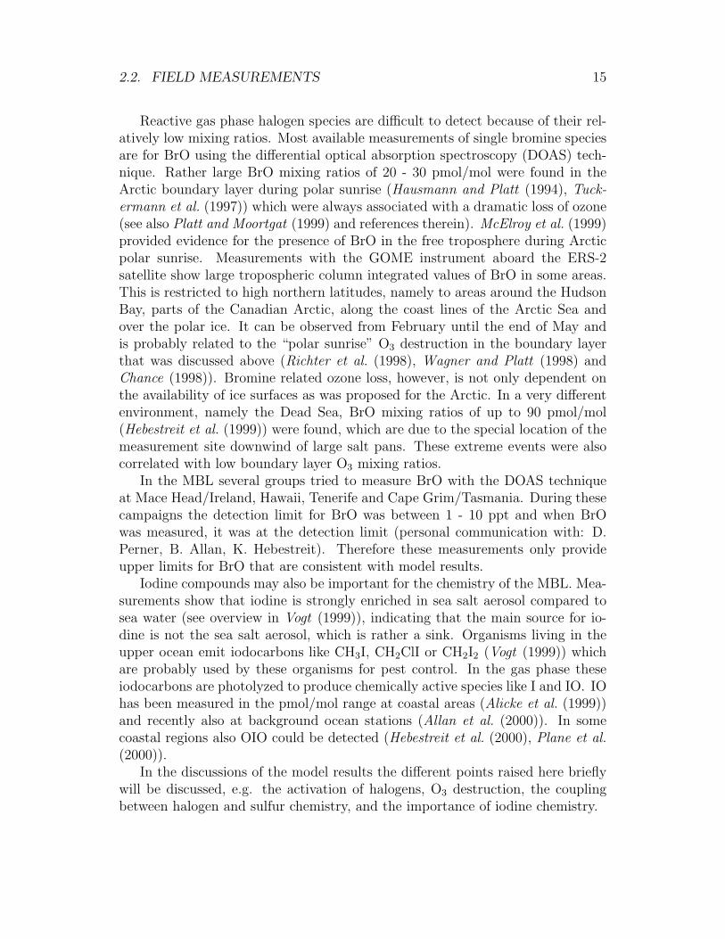
Reactive gas phase halogen species are difficult to detect because of their rel-atively low mixing ratios. Most available measurements of single bromine speciesare for BrO using the differential optical absorption spectroscopy (DOAS) tech-nique. Rather large BrO mixing ratios of 20 - 30 pmol/mol were found in theArctic boundary layer during polar sunrise (Hausmann and Platt (1994), Tuck-ermann et al. (1997)) which were always associated with a dramatic loss of ozone(see also Platt and Moortgat (1999) and references therein). McElroy et al. (1999)provided evidence for the presence of BrO in the free troposphere during Arcticpolar sunrise. Measurements with the GOME instrument aboard the ERS-2satellite show large tropospheric column integrated values of BrO in some areas.This is restricted to high northern latitudes, namely to areas around the HudsonBay, parts of the Canadian Arctic, along the coast lines of the Arctic Sea andover the polar ice. It can be observed from February until the end of May andis probably related to the “polar sunrise” O3 destruction in the boundary layerthat was discussed above (Richter et al. (1998), Wagner and Platt (1998) andChance (1998)). Bromine related ozone loss, however, is not only dependent onthe availability of ice surfaces as was proposed for the Arctic. In a very differentenvironment, namely the Dead Sea, BrO mixing ratios of up to 90 pmol/mol(Hebestreit et al. (1999)) were found, which are due to the special location of themeasurement site downwind of large salt pans. These extreme events were alsocorrelated with low boundary layer O3 mixing ratios.

In the MBL several groups tried to measure BrO with the DOAS techniqueat Mace Head/Ireland, Hawaii, Tenerife and Cape Grim/Tasmania. During thesecampaigns the detection limit for BrO was between 1 - 10 ppt and when BrOwas measured, it was at the detection limit (personal communication with: D.Perner, B. Allan, K. Hebestreit). Therefore these measurements only provideupper limits for BrO that are consistent with model results.

Iodine compounds may also be important for the chemistry of the MBL. Mea-surements show that iodine is strongly enriched in sea salt aerosol compared tosea water (see overview in Vogt (1999)), indicating that the main source for io-dine is not the sea salt aerosol, which is rather a sink. Organisms living in theupper ocean emit iodocarbons like CH3I, CH2ClI or CH2I2 (Vogt (1999)) whichare probably used by these organisms for pest control. In the gas phase theseiodocarbons are photolyzed to produce chemically active species like I and IO. IOhas been measured in the pmol/mol range at coastal areas (Alicke et al. (1999))and recently also at background ocean stations (Allan et al. (2000)). In somecoastal regions also OIO could be detected (Hebestreit et al. (2000), Plane et al.(2000)).

In the discussions of the model results the different points raised here brieflywill be discussed, e.g. the activation of halogens, O3 destruction, the couplingbetween halogen and sulfur chemistry, and the importance of iodine chemistry.

Chapter 3

Description of the MBL model

3.1 Meteorology, microphysics and thermody-

namics

For this modeling study a one-dimensional model is used. The meteorologicaland microphysical part is the boundary layer model MISTRA described in detailby Bott et al. (1996) and Bott (1997). Apart from dynamics and thermodynam-ics it includes a detailed microphysical module that calculates particle growthexplicitly and treats feedbacks between radiation and particles. Figure 3.1 showsschematically the most important processes that are included in the model for acloudy MBL. Gas phase chemistry is active in all model layers, aerosol chemistryonly in layers where the relative humidity (of which a typical vertical profile isshown) is greater than the deliquescence / crystallization humidity (see discus-sion on page 21). When a cloud forms, cloud droplet chemistry is also active.Fluxes of sea salt aerosol and gases from the ocean are included and the mainmeteorological processes (turbulence, radiation) are also shown.

The set of prognostic variables comprises the horizontal components of thewind speed u, v, the specific humidity q, and the potential temperature Θ:

∂u

∂t= −w∂u

∂z+

∂

∂z

(Km

∂u

∂z

)+ f(v − vg) (3.1)

∂v

∂t= −w∂v

∂z+

∂

∂z

(Km

∂v

∂z

)− f(u− ug) (3.2)

∂q

∂t= −w∂q

∂z+

∂

∂z

(Kh

∂q

∂z

)+C

ρ(3.3)

∂Θ

∂t= −w∂Θ

∂z+

∂

∂z

(Kh

∂Θ

∂z

)−(p0

p

)R/cp 1

cpρ

(∂En∂z

+ LC

)(3.4)

where f is the Coriolis parameter, ug and vg are the geostrophic wind components,Km and Kh are the turbulent exchange coefficients for momentum and heat, Lis the latent heat of condensation, C the condensation rate, ρ the air density, p

16

3.1. METEOROLOGY, MICROPHYSICS AND THERMODYNAMICS 17

deli/crys point < RH < 100%

cloudy

sea salt aerosol emissions (DMS, NH3)

chemistry

aerosol

chemistrycloud dropletaerosol and

---> gas phase chemistry in all model domains

subsidence

large scale

radiation

turbulence

turbulence

RH 100%

RH

inversion

ocean

cloud free MBL

FT

Figure 3.1: Schematic depiction of the most important processes included in theone-dimensional boundary layer model MISTRA. The free troposphere is denotedas FT, relative humidity as RH.

the air pressure, p0 the air pressure at the surface, R the gas constant for dry air,cp the specific heat of dry air at constant pressure, and En the net radiative fluxdensity, respectively. The first term on the right of each equation is the large scalesubsidence. Strictly in a one-dimensional framework the vertical velocity w = 0everywhere. To correctly model the evolution of stratiform clouds this termis essential as pointed out by several authors (e.g. Driedonks and Duynkerke(1989)). Mass balance, however, is violated if subsidence is included. In runswhere only aerosol chemistry is studied, i.e. in runs without clouds, the verticalvelocity is set to zero (w = 0) to avoid this problem, for the cloud runs subsidenceis included.

Turbulence is treated with the level 2.5 model of Mellor and Yamada (1982)with the modifications described in Bott et al. (1996). The turbulent exchangecoefficients Km and Kh are calculated via stability functions Sm/h and Gm/h. Theprognostic equation for the turbulence kinetic energy e is:

∂e

∂t= −w∂e

∂z+

∂

∂z

(Ke

∂e

∂z

)+

(2e)3/2

l

(SmGm + ShGh −

1

16.6

)(3.5)

assuming a constant dissipation ratio (last term on the right). For more detailsand an explanation of the calculation of the mixing length l, the exchange coef-

18 CHAPTER 3. DESCRIPTION OF THE MBL MODEL

II

I III

IV

Figure 3.2: The two-dimensional particle spectrum as function of the dry aerosolradius a and the total particle radius r. Added are the chemical bins. I: sulfateaerosol bin, II: sea salt aerosol bin, III: sulfate cloud droplet bin, IV: sea saltdroplet bin. For simplicity a 35 x 35 bin grid is plotted, in the model 70 x 70bins are used.

ficient Ke for the turbulent kinetic energy, and the functions Sm/h and Gm/h seeMellor and Yamada (1982) and Bott et al. (1996).

The microphysics is treated using a joint two-dimensional particle size distri-bution function f(a, r) with the total particle radius r and the dry aerosol radiusa the particles would have, when no water were present in the particles. Thetwo-dimensional particle grid (see Figure 3.2) is divided into 70 logarithmicallyequidistant spaced dry aerosol classes, with the minimum aerosol radius being0.01 µm and the maximum radius 15 µm. Chosing these values allows to accountfor all accumulation mode particles and most of the coarse particles.

Each of the 70 dry aerosol classes is associated with 70 total particle radiusclasses, ranging from the actual dry aerosol radius up to 60 µm (150 µm in cloudruns). The prognostic equation for f(a, r) is:

∂f(a, r)

∂t=

−w∂f(a, r)

∂z+

∂

∂z

(Khρ

∂f(a, r)/ρ

∂z

)− ∂

∂z

(wtf(a, r)

)− ∂

∂r

(rf(a, r)

).

(3.6)

Again, subsidence is the first term on the right, followed by turbulent mixing,particle sedimentation (wt is the sedimentation velocity) and changes in f due toparticle growth (r = dr/dt). Upon model initialization the particles are initializedwith a water coating according to the equilibrium radius of the dry nucleus at theambient relative humidity. During the integration, particle growth is calculated

3.2. CHEMISTRY 19

explicitly for each bin of the 2D particle spectrum using the growth equation afterDavies (1985) (see also Bott et al. (1996)):

rd r

d t=

1

C1

[C2

(S∞Sr− 1

)− Fd(a, r)−mw(a, r)cwdT/dt

4πr

](3.7)

with the ambient supersaturation S∞ and the supersaturation at the droplet’ssurface Sr according to the Kohler equation:

Sr = exp

[A

r− Ba3

r3 − a3

]. (3.8)

The change in particle radius is not determined by changes in water vapor satu-ration alone, but also by the net radiative flux at the particle’s surface Fd(a, r).The constants C1 and C2 in eq. (3.7) are:

C1 = ρwL+ρwC2

D′vSrρsC2 = k′T

[L

RvT− 1

]−1

, (3.9)

mw(a, r) is the liquid water mass of the particle, cw and ρw are the specific heatand density of water, ρs is the saturation vapor density and Rv the specific gasconstant for water vapor. The thermal conductivity k′ of moist air and thediffusivity of water vapor D′v have been corrected for gas kinetic effects followingPruppacher and Klett (1997). The condensation rate C in eq. (3.4) is determineddiagnostically from the partical growth equation.

Collision-coalescence processes are not included in the model because thisleads to great difficulties for describing the redistribution of the chemical speciesin the particles. However a version of MISTRA including collision-coalescencewithout considering chemistry does exist (Bott (2000)).

For the calculation of the radiative fluxes a δ-two stream approach is used(Zdunkowski et al. (1982), Loughlin et al. (1997)). The radiative fluxes are usedfor calculating heating rates and the effect of radiation on particle growth. Theradiation field is calculated with the aerosol/cloud particle data from the micro-physical part of the model, so feedbacks between radiation and particle growthare fully implemented.

3.2 Chemistry

The multiphase chemistry module comprises chemical reactions in the gas phaseas well as in aerosol and cloud particles. Transfer between gas and aqueous phaseand surface reactions on particles are also included. Tables D.1 to D.5 show acomplete listing of the reactions. The reaction set is an updated version of Sanderand Crutzen (1996) (see also http://www.mpch-mainz.mpg.de/˜sander/mocca)plus some organic reactions from Lurmann et al. (1986). In the following the term


aqueous phase is used as generic term for sub-cloud aerosol, interstitial aerosol,and cloud particles.

The prognostic equation for the concentration of a gas phase chemical speciescg (in mol/m3

air) including subsidence, turbulent exchange, deposition on theocean surface, chemical production and destruction, emission and exchange withthe aqueous phases is:

∂cg∂t

= −w∂cg∂z

+∂

∂z

(Khρ

∂cg/ρ

∂z

)− ∂

∂t(vdryg cg)

+P −Dcg + E −nkc∑i=1

[kt,i

(wl,icg −

ca,ikccH

)].

(3.10)

Again subsidence is included only in runs with clouds. P and D are chemicalproduction and destruction terms, respectively, kccH is the dimensionless Henryconstant obtained by kccH = kHRT , where kH is in mol/(m3Pa), wl,i is the di-mensionless liquid water content (m3

aq/m3air) of bin i (see explanation on p. 21).

The emission flux E as well as dry deposition (third term in eq. (3.10)) are ef-fective only in the lowermost model layer. The calculation of the dry depositionvelocity vdryg is explained at the end of this section. The last term in eq. (3.10)describes the transport from the gas phase into the aqueous phases according tothe formulation by Schwartz (1986) (see also Sander (1999)), nkc is the numberof the aqueous classes as explained below. For a single particle, the mass transfercoefficient kt is defined as

kt =

(r2

3Dg

+4r

3vα

)−1

(3.11)

with the particle radius r, the mean molecular speed v =√

8RT/(Mπ) (M is themolar mass), the accommodation coefficient α (see Table D.5), and the gas phasediffusion coefficient Dg. Dg is approximated as Dg = λv/3 (Gombosi (1994), p.125) using the mean free path length λ.

Chameides (1984) points out that the time needed to establish equilibriumbetween the gas and aqueous phase differs greatly for individual species andthat soluble species never reach equilibrium in cloud droplets, emphasizing theimportance of describing phase transfer in the kinetic form that is used here.

Ambient particle populations are never monodisperse, i.e. one has to accountfor particle with different radii. The mean transfer coefficient kt for a particlepopulation is given by the integral:

kt =4π

3wl

logrmax∫logrmin

(r2

3Dg

+4r

3vα

)−1

r3 ∂N

∂logrdlogr. (3.12)

Aqueous chemistry is calculated in four bins (see Figure 3.2): deliquescentaerosol particles with a dry radius less than 0.5 µm are included in the “sulfate

3.2. CHEMISTRY 21

aerosol” bin, whereas deliquescent particles with a dry aerosol radius greater than0.5 µm are in the “sea salt aerosol” bin. Although the composition of the particleschanges over time the terms “sulfate” and “sea salt” aerosol are used to describethe origin of the particles. The particles get internally mixed by exchange with thegas phase but, as mentioned earlier, not by particle collisions. For the descriptionof the initial composition of the aerosol bins see section 4.1.

When the total particle radius exceeds the dry particle radius by a factorof 10, i.e. when the total particle volume is 1000 times greater than the dryaerosol volume, the particle and its associated chemical species are moved tothe corresponding sea salt or sulfate derived cloud particle class. This thresholdroughly coincides with the critical radius derived from the Kohler equation. Whenparticles shrink they are redistributed from the droplet to the aerosol bins.

Therefore in a cloud-free layer there are 2 (nkc = 2) aqueous chemistry classes(sulfate and sea salt aerosol) and in a cloudy layer 2 cloud droplet (sulfate and seasalt derived) and 2 interstitial aerosol (sulfate and sea salt) classes, giving a totalof 4 (nkc = 4) aqueous chemistry classes. In each of these classes the followingprognostic equation is solved for each chemical species ca,i (in mol/m3

air), wherethe index i stands for the i-th aqueous class:

∂ca,i∂t

= −w∂ca,i∂z

+∂

∂z

(Khρ

∂ca,i/ρ

∂z

)− ∂

∂t(vdrya,i ca,i)

+P −Dca,i + E + Ppc + kt,i

(wl,icg −

ca,ikccH

) (3.13)

The individual terms have similar meanings as in eq. (3.10). The calculationof the sedimentation velocity vdrya,i is explained at the end of this section. Theadditional term Ppc accounts for the transport of chemical species from the aerosolto the cloud droplet regimes and vice versa. If only phase transfer is considered,this equation reduces in steady state conditions (∂ca,i/∂t = 0) to the Henryequilibrium ca,i = wl,icgk

ccH .

The concentration of H+ ions is calculated like any other species, i.e. nofurther assumptions are made. The charge balance (sometimes used to derive thepH) is satisfied implicitly.

Cloud-processing, i.e. the change of aerosol mass due to uptake of gases, isincluded in the model based on Bott (1999).

It is assumed that water is associated with sea salt aerosol particles abovetheir crystallization point rather than their deliquescence point because they areproduced as droplets at the sea surface. Therefore the hysteresis effect ensuresthat, upon drying, the particles remain in a metastable highly concentrated solu-tion state above their crystallization point, which is about 45 % relative humidityfor NaCl (Shaw and Rood (1990), Tang (1997), Pruppacher and Klett (1997), andLee and Hsu (2000)). As long as the relative humidity in the MBL is well abovethe crystallization point, sea salt aerosol is not present in crystalline form.

The crystallization humidity for many mixed aerosol particles containing sul-fate or nitrate is below 40 % relative humidity (Seinfeld and Pandis (1998) and


references therein), implying that aerosol particles that already had been involvedin cloud cycles will also be in an aqueous metastable state. Therefore many sol-uble aerosol particles will be present in the atmosphere as metastable aqueousparticles below their deliquescence humidity. A relative humidity of 60 % is usedas threshold for sulfate particles to be in aqueous form. With the above discus-sion in mind, this might lead to an underestimation of aqueous sulfate particles,but, at least in the model runs presented here, the ambient relative humidity isalways above 60 %, so all aerosol particles are assumed to be present in aqueousform. The only exception from this is the “high BL” run as discussed in section4.4.

Aerosols are usually highly concentrated solutions. Laboratory measurementsshow that NaCl molalities can be in excess of 10 mol/kg (Tang (1997)) implyingalso very high ionic strengths. Therefore it is necessary to account for deviationsfrom ideal behaviour, i.e. to include activity coefficients. The Pitzer formal-ism (Pitzer (1991)) is used to calculate the activity coefficients for the actualcomposition of each aqueous size bin.

In the atmosphere each aerosol or cloud particle is a closed “reaction chamber”with its own pH and concentrations of the species. In models the particles have tobe lumped in bins where the individual properties of the particles vanish. In themodel freshly emitted, alkaline sea salt particles are put into the same chemistrybin as aged acidic particles leading to mean conditions and reaction paths thatcan be distinctly different from what is happening in the atmosphere. Especiallyin the case of high wind, when sea salt aerosol production and therefore alsosea salt aerosol loadings are high, the pH might be overestimated and reactionsinvolving acidity might be underestimated because the buffer capacity of thefew large particles would dominate the smaller, more acidic particles. In futureversions of this model a finer resolution for the aqueous chemistry bins will beachieved.

Photolysis is calculated online using the method of Landgraf and Crutzen(1998). The photolysis rate (or photo dissociation coefficient) JX for a gas X canbe calculated from the spectral actinic flux F (λ) via the integral:

JX =

∫I

σX(λ)φX(λ)F (λ)dλ (3.14)

where λ is the wavelength, σX the absorption cross section, φX the quantum yieldand I the photochemically active spectral interval. If the integral in eq. (3.14)would be approximated with a sum, the number of wavelength bins needed for anaccurate approximation of the integral would be in the order of 100 which wouldlead to excessive computing times. Landgraf and Crutzen (1998) suggested amethod using only 8 spectral bins (see Table 3.1) approximating (3.14) by:

JX ≈8∑i=1

Jai,X · δi (3.15)

3.2. CHEMISTRY 23

Table 3.1: Subdivision of the spectral range of the photolysis module.

interval 1 2 3 4 5 6 7 8λa [nm] 178.6 202.0 241.0 289.9 305.5 313.5 337.5 422.5λb [nm] 202.0 241.0 289.9 305.5 313.5 337.5 422.5 752.5λi [nm] see LC98 205.1 287.9 302.0 309.0 320.0 370.0 580.0

The spectral range 178.6 nm ≤ λ ≤ 752.5 nm is subdivided into eight intervals, λa andλb are the initial and the final, and λi the fixed wavelength in interval Ii (after Landgraf andCrutzen (1998)). The intervals 1 and 2 are important only for the stratosphere, as only light withwavelengths greater than about 290 nm reaches the troposphere.

where Jai,X is the photolysis rate for a purely absorbing atmosphere. The factorδi:

δi :=F (λi)

F a(λi)(3.16)

describes the effect of scattering by air molecules, aerosol and cloud particles,which is significant in the spectral range 202.0 nm ≤ λ ≤ 752.5 nm. F a(λi) is theactinic flux of a purely absorbing atmosphere. For the Schumann-Runge band(spectral range 178.9 nm ≤ λ ≤ 202.0 nm), scattering effects can be neglectedbecause of the strong absorption by O2 (δ1 = 1). The factor δi is calculated onlinefor one wavelength for each interval (see λi in Table 3.1).

The Jai,X are precalculated with a fine spectral resolution and are approximatedduring runtime from lookup tables or by using polynomials. The advantage ofthis procedure is that the fine absorption structures that are present in σX andφX are considered and only Rayleigh and cloud scattering, included in F (λi), aretreated with a coarse spectral resolution which is justified.

For the calculation of the actinic fluxes a four stream radiation code is usedin addition to the two stream radiation code used for the determination of thenet radiative flux density En because different spectral resolutions and accuraciesare needed for these different purposes. Based on the findings of Ruggaber et al.(1997) a factor 2 is applied to photolysis rates inside aqueous particles to accountfor the actinic flux enhancement inside the particles due to multiple scattering.

All chemical reactions in gas and aqueous phases, equilibria and phase transferreactions are calculated as one coupled system using the kinetic preprocessor KPP(Damian-Iordache (1996)) which allows rapid change of the chemical mechanismwithout major changes in the source code.

Constant emission fluxes for the gases DMS and NH3 from the sea surface areapplied with 2×109 molec/(cm2s) (Quinn et al. (1990)) and 4×108 molec/(cm2s)(Quinn et al. (1990), scaled to model their measured gas phase mixing ratios of19 noml/mol in clean air masses), respectively.

Sea salt particles are emitted by bursting bubbles at the sea surface (e.g.Woodcock et al. (1953), Pruppacher and Klett (1997)). The parameterization ofMonahan et al. (1986) is used that estimates the flux F of particles with radius


r at a relative humidity of 80 % per unit area of sea surface, per increment ofdroplet radius and time (in particles m−2 s−1 µm−1):

dF

dr= 1.373u3.41

10 r−3(1 + 0.057r1.05)× 101.19exp(−B2) (3.17)

where B = (0.380−log r)/0.65 and u10 is the windspeed at 10 m height. Monahanet al. (1986) also parameterize the emission for particles with radii larger thanr=10 µm by additional terms, but only the bubble burst mechanism and notthe spume production terms are included because as pointed out by e.g. Wu(1993), Gong et al. (1997) and Andreas (1998) these additional terms lead to anoverestimation of the particle flux compared to measurements.

Large sea spray droplets (r=10 – 300 µm) can contribute to the transport ofheat and moisture between ocean and atmosphere. According to Andreas et al.(1995) this is important for high windspeeds above about 15 m/s. As the modelstudies are mainly for moderate wind speeds where only very small amounts ofparticles of that size are produced this process is neglected.

For each dry aerosol radius bin of the 2D microphysical spectrum the equi-librium radius for the actual relative humidity is calculated and the appropriatenumber of particles according to eq. (3.17) is added in the lowermost model layer.The Monahan et al. (1986) estimate of the sea salt aerosol flux based on windtunnel experiments is believed to yield good results for small particles (Andreas(1998)). For higher wind speeds the resulting mass flux of sea salt particles isless realistic, so for the model runs with high wind speed the parameterization ofSmith et al. (1993) that is based on measurements off the Scottish coast is used.

The dry deposition velocity for gases vdryg at the sea surface is calculated usingthe resistance model described by Wesely (1989):

vdryg =1

ra + rb + rc. (3.18)

The aerodynamic resistance ra is calculated using:

ra =1

κu∗

[ln

(z

z0

)+Φs(z, L)

], (3.19)

with the friction velocity u∗, the von Karman constant κ = 0.4, and the stabilityfunction Φs which depends on the Monin-Obukhov length L, the roughness lengthz0 and a reference height z. The quasi-laminar layer resistance rb is parameterizedas:

rb =1

u∗(Sc−2/3 + 10−3/St). (3.20)

The Stokes number St can be written as St = wtu2∗/(gν) and the Schmidt number

as Sc = ν/D with the dynamic viscosity of air ν and the aerosol diffusivity D.

3.3. MODEL RESOLUTION AND INTEGRATION SCHEME 25

The surface resistance rc is calculated using the formula by Seinfeld and Pandis(1998) (their equation (19.30)):

rc =2.54 ∗ 104

H∗Tu∗, (3.21)

with the effective Henry constant H∗.The dry deposition velocity of particles vdrya,i is calculated after Seinfeld and Pandis(1998):

vdrya,i =

{1

ra+rb+rarbwt+ wt lowest model layer

wt rest of model domain. (3.22)

The particle sedimentation velocity wt is calculated in the microphysical moduleassuming Stokes flow and taking into account the Cunningham slip flow correctionfor particles with r < 10µm and after Beard for larger particles (see Pruppacherand Klett (1997)).

3.3 Model resolution and integration scheme

The atmosphere between the sea surface and 2000 m is divided into 150 layers.The lowest 100 layers have a constant grid height of 10 m, the layers above 1000 mare spaced logarithmically. For the “high boundary layer” run the grid height inthe lowest 100 layers was increased to 20 m and the model domain was extendedto 3500 m.

The dynamical timestep is 10 s and the chemical timestep is chosen to dif-fer between 1 ms for layers with low LWC associated to the particles or layersincluding freshly formed particles and 60 s for gas phase only layers.

The very stiff chemical differential equation system is solved with a secondorder Rosenbrock method (ROS2 by Verwer et al. (1997)).

Chapter 4

Chemistry of the cloud-free MBL

4.1 Overview of the runs

With the base run for the study of aerosol chemistry (i.e. without clouds) it wasnot intended to mimic a situation that has been observed in a field campaign, itis rather intended to demonstrate the evolution of the gas and aerosol chemistryunder idealized conditions. The latitude chosen for this run is ϕ = 30◦ at the endof July. The boundary layer height is roughly 700 m, moisture and heat fluxesfrom the sea surface are adjusted to yield a stable boundary layer. The relativehumidity at the sea surface is roughly 65 %, increasing to around 90 % below theinversion that caps the MBL. As a result of the prescribed heat fluxes from thesea surface, the potential temperature in the well mixed MBL is slowly decreasingfrom Θ = 14.5◦C to 13.5 ◦C. The relative humidity in the different layers staysconstant apart from a minor diurnal variation (±3%). After a spin-up of thedynamical part of the model for 2 days the complete model was integrated for 3days.

Many different sensitivity studies were performed and some of them and thedifferences between them are described here. See Table 4.3 for an overview of theruns.

First the halogen chemistry was turned off in the run “halogen off” and inanother run both, halogen and aerosol chemistry (“aerosol off”) were switchedoff. In the run “low O3 low SO2” low initial values for these gases were chosenin the initialization of the run to see the effects of very clean air. The contrarywas simulated at with the “continental influence” run where high initial values ofNOx, SO2, O3 and other pollutants were chosen. To see the influence of the seasona “winter” and a “spring” run were performed. The implications of differentheights of the MBL were the object of the “high BL” run. In the run “strongwind” the wind speed and the parameterization of the sea salt aerosol productionwere changed to study the effects of the production of more and larger particlesat higher wind speeds. Higher mean wind speeds over the ocean could be aconsequence of global change with impacts on chemistry and microphysics in theMBL as already mentioned by Pszenny et al. (1998). The strength of the DMSflux was varied in the “high DMS” run and iodine chemistry was included in the

26

4.1. OVERVIEW OF THE RUNS 27

Table 4.1: Initial mixing ratios of gas phase species (in nmol/mol).

species remote (MBL) remote (FT) cont. influen. (MBL) cont. influen. (FT)CO 70.0 150.0NO2 0.02 0.03 0.5HNO3 0.01 0.05 0.1NH3 0.08 0.2SO2 0.09 1.0O3 20.0 50.0 50.0 70.0CH4 1800.0 1800.0C2H6 0.5 5.0HCHO 0.3 0.3H2O2 0.6 0.8PAN 0.01 0.1 0.1 1.0HCL 0.04 0.04DMS 0.06 0.06CH3I 0.002C3H7I 0.001

Values are for the 2 scenarios “remote” and “continentally influenced”. A value for thefree troposphere (FT) is given only when it is different from the MBL value. CH3I and C3H7Iare accounted for only in the “iodine” run.

Table 4.2: Initial size distribution of the aerosol.

mode Ntot,i

(1/cm3)RN,i (µm) σi

1 100 0.027 1.7782 120 0.105 1.2943 6 0.12 2.818

The data is after Hoppel and Frick (1990). The particle size distribution is calculated

according to dN(r)dlgr =

∑3i=1

Ntot,ilgσi√

2π× exp

(− (lgr−lgRN,i)2

2(lgσi)2

).

“iodine” run.

Tables 4.1 and 4.2 list the initial gas phase mixing ratios and parameters forthe initial lognormal aerosol size distribution. Aerosol particles with dry radii lessthan r=0.5 µm are assumed to be a mixture of 32 % (NH4)2SO4, 64 % NH4HSO4

and 4 % NH4NO3 (Kim et al. (1995)).

The resulting pH of the sulfate aerosols is between 0.5 and 1 (and even lowerfor the “continentally influenced” run) which is in the range estimated by Fridlindand Jacobson (2000) for sulfate aerosol sampled during the ACE-1 campaign. Arun where the initial composition of the sulfate aerosol was assumed to be pure(NH4)2SO4 showed a pH between 2.5 at model start and 1 after 3 days due tothe uptake of acids the gas phase. Consequences for the gas phase were verysmall, NH3 increased because of reduced uptake by the sulfate aerosol whereasHCl decreased due to uptake by the sulfate aerosol.

28 CHAPTER 4. CHEMISTRY OF THE CLOUD-FREE MBL

Tab

le4.

3:O

verv

iew

ofth

ese

nsi

tivit

yru

ns

for

the

clou

d-f

ree

MB

L.

nam

ega

sph

ase

init

ializ

atio

n(s

eeT

able

4.1)

MB

Lhe

ight

SST

Diff

eren

ces

from

base

run

Mai

nre

sult

s

base

run

rem

ote

700m

15◦ C

-B

rOve

rtic

alpr

ofile

/diu

rnal

vari

-at

ion,

vert

ical

profi

leof

sea

salt

pH,

recy

clin

gof

HB

ran

dH

OB

rby

sulfa

te,

“ove

rall”

effec

tsof

halo

gen

chem

istr

yha

loge

noff

rem

ote

700m

15◦ C

halo

gen

chem

istr

ysw

itch

edoff

over

all

impo

rtan

ceof

halo

gen

chem

istr

ysh

own

aero

sol

offre

mot

e70

0m15◦ C

halo

gen

and

aero

solc

hem

istr

ysw

itch

edoff

over

all

impo

rtan

ceof

aero

sol

chem

istr

ysh

own

low

O3

low

SO2

rem

ote,

but

O3

=12

nmol

/mol

,SO

2=

20pm

ol/m

ol

700m

15◦ C

gas

phas

ein

itia

lizat

ion

low

O3

redu

ces

Br

acti

vati

on,i

ni-

tial

mix

ing

rati

osof

SO2

unim

-po

rtan

tfo

rst

eady

stat

eco

ndi-

tion

slo

wO

3lo

wSO

2la

rge

sulfa

tesu

rfac

esa

me

as“l

owO

3lo

wSO

2”

700m

15◦ C

sulfa

teae

roso

lmod

era

dius

in-

crea

sed

byfa

ctor

1.5

recy

clin

gof

HB

r,H

OB

rby

sulfa

teae

roso

lis

impo

rtan

tco

ntin

enta

lin

fluen

ceco

ntin

enta

llyin

fluen

ced

700m

15◦ C

gas

phas

ein

itia

lizat

ion

quic

ker

Br

acti

vati

onw

inte

rre

mot

e75

0m5◦ C

sola

rde

clin

atio

n-2

0◦

inst

ead

of20◦

high

erB

rOm

ixin

gra

tios

than

insu

mm

ersp

ring

rem

ote

700m

10◦ C

sola

rde

clin

atio

n0◦

inst

ead

of20◦

sim

ilar

tow

inte

r

high

BL

rem

ote

1300

m15◦ C

inve

rsio

nat

1300

min

stea

dof

750m

,ve

rtic

alre

solu

tion

20m

impo

rtan

ceof

recy

clin

gby

sulfa

teae

roso

l,le

ssst

rong

Br x

acti

vati

onst

rong

win

dre

mot

e70

0m15◦ C

u 10≈

9m

/s(i

nste

adof

6m

/s),

sea

salt

aero

solfl

uxpa

ram

.by

Smit

het

al.

(199

3)

stro

ngin

crea

sein

S(IV

)ox

idat

ion

inse

asa

ltpa

rtic

les

carb

onat

ere

mot

e70

0m15◦ C

carb

onat

ebu

ffer

inse

asa

ltin

crea

sed

by50

%(S

ieve

ring

etal

.(1

999)

)

chan

ges

inim

port

ance

ofS(

IV)

oxid

atio

npa

ths

iodi

nere

mot

e70

0m15◦ C

iodi

nech

emis

try

incl

uded

quic

ker

Br

acti

vati

onan

dgr

eate

rO

3lo

ss

SST

isth

ese

asu

rfac

ete

mpe

ratu

re.

Furt

her

deta

ilson

the

char

acte

rist

ics

ofth

eba

seru

nar

egi

ven

inse

ctio

n(4

.1).

4.2. HALOGEN ACTIVATION 29

Particles larger than r=0.5 µm are assumed to be sea salt particles. Thecomposition of sea salt aerosol in the model differs somewhat from the sea watercomposition in Table 1.1, because in the model only Na+ is considered as cationbecause the cations are chemically unreactive in the atmospheric aerosol. Theanions considered are Cl−, Br−, HCO−3 and for the iodine run also I− and IO−3 .Sulfate is not considered as initial component of sea salt aerosol as it is alsoassumed to be chemically unreactive. Therefore all sulfate that is present in seasalt aerosol in the model runs stems from uptake from the gas phase and canbe labelled “non-sea salt sulfate”. According to these assumptions, the molarratio of Br− to Na+ (used as the sum of cations in sea water) is about 1 : 640and HCO−3 : Na+ = 1 : 235 (see also Sander and Crutzen (1996)). Upon modelinitialization “fresh” sea salt with a pH of about 8 is present everywhere in theMBL. Uptake of acidic gases like HNO3 from the gas phase rapidly acidifies thesea salt aerosol particles. When fresh sea salt aerosols are emitted from the seasurface they also have a pH around 8.

4.2 Halogen activation

The model runs start at midnight. Figure 4.1 shows the evolution with time ofmajor gas phase species for the base run, the “continental influence” run andthe “low O3 low SO2” run. Shortly after model start the sea salt aerosol isacidified due to rapid uptake of acids from the gas phase (see Figure 4.2) with pHvalues ranging between 6 at the surface and less than 3.5 at the top of the MBL(see Figure 4.9 for a depiction and section 4.10 for a discussion of the verticalprofile of the sea salt aerosol pH). At the surface fresh alkaline sea salt aerosolis continuously emitted which is added to the pre-existing sea salt particles inthe lowest model layer resulting in a mixture of old acidified and fresh alkalineparticles. The acidification of the sea salt particles is an important step in thereaction cycles, because many of them are acid catalyzed.

The halogen chemistry is started by reactions that transform Br− into speciesthat can degas from the aerosol and initiate quick reaction cycles in the gas phase.These starter reactions are reactions of Br− with OH, HSO−5 and NO3 (reactionsA49, A107, A50).

The reaction cycles responsible in the model for the degassing of the reactivebromine species (Br2 and BrCl) involve the following steps as discussed in Sanderand Crutzen (1996) and Vogt et al. (1996) (see also Figure G.1 for an overviewof the most important bromine reactions):

HOBr ←→ HOBraq (I.1)

HOBraq + Cl− +H+ ←→ BrClaq +H2O (I.2)

Depending on the concentrations of the species involved in aqueous phase equi-libria BrClaq either degasses (when significant Br− depletion has occured) and isthen photolysed:


BrCl + hν −→ Br + Cl λ < 560nm (I.3)

or takes part in the following autocatalytic cycles (when sufficient Br− is available)leading to the production of Br2:

BrClaq +Br− ←→ Br2Cl− (I.4)

Br2Cl− ←→ Br2aq + Cl− (I.5)

Br2aq ←→ Br2 (I.6)

Br2 + hν −→ 2Br λ < 600nm (I.7)

2(Br +O3) −→ 2(BrO +O2) (I.8)

2(BrO +HO2) −→ 2(HOBr +O2) (I.9)

Or instead of equilibria (I.2), (I.4) and (I.5):

HOBraq +Br− +H+ ←→ Br2aq +H2O (I.10)

leading in both cases to the following net reaction:

2HO2 +H+ + 2O3 +Br− + hνHOBr,Cl−−→ HOBr + 4O2 +H2O (I.11)

This autocatalytic bromine activation cycle consumes H+ ions which implies theneed for acidification of the sea salt aerosol as shown by Fickert et al. (1999) inlaboratory experiments.

Keene et al. (1998) studied the influence of the pH on halogen activation. Theyshowed that significant sea salt dehalogenation is limited to acidified aerosol butthat differences between a pH of 5.5 and 3 are not significant.

Sander et al. (1999) showed that when sufficient NOx is available, reactionson the surface of aerosols can also lead to the production of Br2 and BrCl withoutthe need for acid catalysis:

BrO +NO2M−→ BrNO3 (II.1)

BrNO3H2O−→ HNO3aq +HOBraq (II.2)

BrNO3Cl−−→ NO−3 +BrClaq (II.3)

BrNO3Br−−→ NO−3 +Br2aq (II.4)

The uptake of BrNO3 is followed by conversion of HOBr as shown in cycle (I)and the degassing of Br2 and BrCl.


Figure 4.1: Evolution with time of the main gas phase species for the base run(solid line), the “continental influence” run (dotted line) and the “low O3 lowSO2” run (dashed line) (in 50 m). Clx (Brx) is the sum of all gas phase chlorine(bromine) species except HCl (HBr).


Figure 4.1: Continued.


Figure 4.2: Evolution with time of some aqueous phase species as well as liquidwater content (LWC) and pH for the base run (solid line), the “continental in-fluence” run (dotted line) and the “low O3 low SO2” run (dashed line) in 415 mheight in the sulfate and sea salt aerosol. LWC is the liquid water content, unitsare mol/m3

air.

These reaction cycles lead to gradual build-up of total reactive bromine Brx

(the sum of all gas phase bromine species except HBr) in the gas phase withmaximum values between 8 and 10 pmol/mol in the model runs. During daylightthe main Br species are HOBr, HBr and BrO, during night this is shifted towardsBr2 and BrCl that are photolyzed readily during daylight (see Figure 4.1). Modelcalculated bromide deficits are between 70 and 85 % in 50m height, rising to 90- 99 % in higher model layers due to the lower sea salt aerosol pH in that layers(see section 4.10).


The gas phase mixing ratio of O3 is important for these cycles because theproduction of BrO and therefore also the O3 destruction is catalyzed by O3 (re-action (I.8). If O3 mixing ratios are small, halogen activation is slowed down (seerun “low O3 low SO2”).

The order of magnitude of total inorganic gas phase bromine (Brt = Brx +HBr) in the model is in the range of the measurements of total inorganic gasphase bromine by Rancher and Kritz (1980) that were made during a cruise offthe equatorial African coast. The measured daytime gas phase concentrations areabout twice the night time values whereas daytime concentrations of particulatebromine were about half the nighttime values. They suggested that there mightbe a reversible day-night exchange between particulate and gas phase. In themodel this diurnal variation cannot be found, total inorganic gas phase brominepeaks at sunrise and has a minimum before sunset. The difference between dayand night mixing ratios is only on the order of 20 % close to the surface and afew percent in higher layers of the MBL. It is caused by photolysis shifting thegas phase species from Br2 and BrCl towards HOBr, BrNO3 and HBr which aretaken up by the aqueous phases.

As mentioned by Rancher and Kritz (1980) the cloud cover during their cruisewas between 0 and 0.5. In model runs that include clouds the model predictsdiurnal variation of Brt that are distinctively different from the ones in runswithout clouds. See section 5 for a discussion of this point and note that othermeasurements did not show a diurnal variation of Brx (Moyers and Duce (1972)).

4.3 Diurnal variation of BrO

The model predicts a distinct diurnal variation of BrO, BrNO3, ClO, and ClNO3

showing a minimum around noon and maxima in the morning and evening (seeFigure 4.1). This feature can be explained by differences in the photolysis spectraof O3 and Br2 and BrCl. The wavelength dependence of O3 photolysis is differentfrom that of Br2 and BrCl that are more rapidly photolysed than O3 due toabsorption at longer wavelengths.

At sunrise (high solar zenith angle) the solar spectrum in the lower troposphereis shifted to longer wavelengths resulting in a delay of O3 photolysis relative toBr2 and BrCl (see Figure 4.3). This causes a delay in the photolytically initiatedproduction of OH and HO2 relative to the production of Br. With low HO2 themain sink for BrO (reaction (I.9)) apart from photolysis is slow, leading to anincrease in BrO mixing ratios (producing the morning peak). Later during theday HO2 mixing ratios are sufficiently high to reduce BrO mixing ratios leading tothe noon minimum. During the afternoon a similar mechanism as in the morningleads to the evening peak of BrO.

If the same wavelength dependence for the photolysis of O3 and Br2 are as-sumed, there is no noon minimum produced by the model but rather a diurnalcycle of BrO that is similar to e.g. OH, showing that the wavelength dependenceof the photolysis of the different species is the cause for the noon minimum in BrO

4.4. ACTIVE RECYCLING OF BRX BY THE SULFATE AEROSOL 35

O

Br

3

2

Figure 4.3: Diurnal variation of the photolysis frequencies for O3 and Br2 (notethe different units). The difference in the shape of the diurnal variation is thecause for the noon minimum in BrO mixing ratios (see text).

and the other affected species. The diurnal variation of BrO is accompanied byan early morning peak in O3 destruction by XO + YO and XO + NO2 reactions(X,Y = Br,Cl).

Nagao et al. (1999) found a “sunrise ozone destruction” (SOD) in the diurnalvariation of O3 based on measurements over a 3-year period on an island in thesub-tropical Northwestern Pacific. This SOD could not be explained by photo-chemistry that neglects halogens. They speculated that bromine spieces mightplay a role in SOD. A similar feature was found by Galbally et al. (2000) in a timeseries of 13 years of O3 observations at Cape Grim, Tasmania. They also founda decrease in O3 concentrations in the first hours after sunrise and speculatedabout the importance of halogens in this additional O3 destruction process.

4.4 Active recycling of Brx by the sulfate aerosol

The presence of sulfate aerosol particles is important for the halogen activationcycle. The large surface area of the sulfate aerosol of 40 to 60 µm2/cm3, comparedto the sea salt surface area of 25 to 45 µm2/cm3, is the reason that HBr, HOBrand BrNO3 are also scavenged to a significant amount by the sulfate aerosol andare involved in reactions on and in sulfate particles. Due to the low pH of thesulfate aerosol the acid catalyzed cycle (I) quickly transforms Br− and Cl− (fromthe dissociation of HBr and HCl) and HOBr to BrCl and Br2 which rapidly degas.As can be seen from Figure 4.4 the magnitude of recycling of bromine species ishigher than in the sea salt aerosol by roughly a factor of 5 to 10. Due to thisrecycling process the sulfate aerosol is not a significant sink for gas phase bromine;some bromine, however, will always be found in the sulfate aerosol.

Particle composition measurements (e.g. Moyers and Duce (1972), Duce et al.(1983)) sometimes (but not always) showed an increase of the bromine to sodium


Figure 4.4: Net exchange of Brx and HBr between sea salt and sulfate aerosoland gas phase (in 215 m). A negative sign implies loss for the aerosol. The solidline is the net flux of Br atoms.

ratio in small particles compared to sea water. Depending on the measurementtechnique some measurements show the ratio of the ions Br−/Na+ whereas oth-

4.5. NIGHTTIME FLUXES OF BROMINE 37

ers show the elemental ratio. The interpretation of this data is difficult becausefor some samples the chemical state of bromine in the particles is unclear. Fur-ther, sodium in the aerosol samples could be a consequence of the sampling ofan external mixture of sulfate and sea salt particles or of internally mixed par-ticles that originate from collision-coalescence or cloud processes (or both). Theenriched bromine could be in the form of stable bromine containing ions or or-ganic molecules. Known reactions (Haag and Hoigne (1983)) for the productionof stable ions like BrO−3 in the aqueous phase are too slow to lead to significantproduction in the aerosol. See also section 5 for a discussion of this topic for thecloud runs.

To further highlight the importance of the sulfate aerosol as active recyclersthe “low O3 low SO2” run was repeated (called “low O3 low SO2 sulf”), with anincrease the particles mode radius of the initial sulfate aerosol by 50 % therebyincreasing the total (dry) sulfate aerosol surface by a factor of 2.25. This led toa strong increase in the recycling of bromine through sulfate aerosol compared tothe base run. After 43 hours Brx was the same as in the base run whereas in the“low O3 low SO2” (with smaller sulfate aerosol particles) this is never achieved.The bromine fluxes of HOBr and HBr to and of Br2 and BrCl from the sulfateaerosol were 3.4 times greater on the second model day compared to the “low O3

low SO2” run and 2 times greater on the third model day.

In the “high BL” run the MBL has a depth of 1250 m, relative humidity atthe sea surface is 50 % increasing to 90 % below the inversion. This implies thatsulfate aerosol chemistry is not active in the lowest 400 m where relative humidityis too small (see page 22). During the day the gas phase mixing ratios of Br2 andBrCl are mainly determined by the flux from the aerosols and loss by photolysis,mixing is much slower than these processes. Br2 and BrCl increase roughly bya factor of ten from the layers without sulfate aerosol chemistry to higher layerswhere it is active. BrNO3 and HOBr decrease by the same absolute amount butthe relative change is smaller due to higher mixing ratios. This points again tothe importance of the sulfate aerosol in recycling these species. Furthermore dueto the low relativ humidity and a stronger vertical dilution the sea salt aerosol pHis quite high, decreasing from 8 near the surface to 6 in 500 m and 4 in 1000 m.This allows rapid bromine release only in the highest layers of the MBL.

4.5 Nighttime fluxes of bromine

During daylight, photolysis is the driving force for the net transport of brominefrom the aqueous to the gas phase as formation of HOBr is dependent on photol-ysis. During night Br2 also degasses as evident from Figure 4.4. This is causedby a sudden rise in BrCl mixing ratios after sunset due to absent photolyticalloss. Thus the gas-aqueous partitioning of these species is perturbed leading tothe reaction sequence:


BrCl −→ BrClaq (III.1)

BrClaq +Br− −→ Br2Cl− (III.2)

Br2Cl− −→ Cl− +Br2aq (III.3)

Br2aq −→ Br2 (III.4)

where in equilibria the net direction is indicated. This cycle results in net transferof Br from the aqueous to the gas phase:

BrCl +Br− −→ Cl− +Br2.

If the bromide depletion in the sea salt aerosol is close to complete, another se-quence gains in importance (in agreement with laboratory experiments of Fickertet al. (1999)):

Br2 −→ Br2aq (IV.1)

Br2aq + Cl− −→ Br2Cl− (IV.2)

Br2Cl− −→ Br− +BrClaq (IV.3)

BrClaq −→ BrCl (IV.4)

The Br− produced in step (IV.3) can then take part in the following reactionsequence:

Cl2 −→ Cl2aq (V.1)

Cl2aq +Br− −→ BrCl−2 (V.2)

BrCl−2 −→ BrClaq + Cl− (V.3)

BrClaq −→ BrCl (V.4)

(V.4)

or in :

HOCl −→ HOClaq (VI.1)

HOCl +Br− +H+ −→ BrClaq +H2O (VI.2)

BrClaq −→ BrCl. (VI.3)

Cycles (IV) and (V) combined give:

Br2 + Cl2 −→ 2BrCl

cycles (IV) and 2 · (VI) combined give:

4.6. EFFECT ON O3 39

Br2 + 2HOCl −→ 2BrCl

i.e. these cycles are no net sink for total gas phase bromine, they just shift gasphase bromine from Br2 to BrCl which is what is observed both in the modelfor the strongly depleted (e.g. “continental influence run”) cases and in thelaboratory (Fickert et al. (1999)).

4.6 Effect on O3

In the remote MBL O3 mixing ratios are believed to be mainly determined bythe mixing ratios of HOx and NOx and by dynamics, i.e. downmixing of O3-richair from the free troposphere (e. g. Monks et al. (2000)). Photochemistry in theremote MBL usually leads to a net photochemical destruction of O3. Here it isshown that halogen radicals can significantly contribute to O3 loss in the MBL.

To properly asses the effect of chemical reactions on O3, the odd oxygen familyOx has been defined (based on Crutzen and Schmailzl (1983)): Ox = O3 + O+ O(1D) + NO2 + 2 · NO3 + 3 · N2O5 + HNO4 + ClO + 2 · Cl2O2 + 2 ·OClO + BrO + IO + 2 · I2O2 (OIO is not included because it is assumed tobe photolytically stable in contrary to OClO). Species in this family are readilytransfered to O3 (e.g. NO2 which photolyses forming O which recombines withO2 to O3). Only if there a reaction leads to a change in the mixing ratio of theodd oxygen family (∆Ox 6= 0) an effective O3 destruction or production tookplace.

Chemical Ox production in the MBL is primarily by reaction of NO withHO2 and CH3OO, both of which form NO2. In the base run it sums up to 1.9nmol/(mol day).

Figure 4.5 shows accumulated rates for the major Ox loss reactions for thebase run, the “continental influence” run, and the “low O3 low SO2” run. Themost important Ox loss reaction is O(1D) + H2O which accounts for 52 % of netO3 destruction followed by O3 + HO2 with 13 %. The main step in brominerelated photochemical O3 destruction is the production of BrO in reaction (I.8)followed by reactions of BrO with HO2, CH3OO, XO (X = Br, Cl) radicals, andNO2. In the base run the halogen related O3 destruction reactions account forroughly 30 % of net O3 destruction.

The most important bromine reaction (BrO + HO2) causes 12 % loss. Chlo-rine related O3 destruction is less important than the bromine reactions, theyaccount together for roughly 4 %.

Most of the reactions depicted in Figure 4.5 show the highest rate for the“continental influence” run and smallest rates for the “low O3 low SO2” run.The relative importance of reactions involving reactions of XO with YO (X, Y= Cl,Br), however, is highest in the base run because there the loss of XO byreaction with NO2 is lower than in the “continental influence” run. This alsoincreases the importance of the BrO + DMS reaction.


Figure 4.5: Accumulated Ox (see definition in section (4.6)) related reaction rates inmol/mol for the base run (solid line), the “continental influence” run (dotted line) andthe “low O3 low SO2” run (dashed line) (in 415 m). Note: for the net plots change inOx is plotted, whereas for the individual reactions the accumulated reaction rates areplotted, i.e. to get ∆Ox from the BrO + BrO reactions multiply with 2.

4.6. EFFECT ON O3 41

Tab

le4.

4:O

3des

truct

ion

rate

s.

run

O(1

D)

+H

2O

O3

+H

O2

O3

+O

HC

lO+

HO

2/

NO

2/

CH

3O

O

BrO

+H

O2

BrO

+C

lOB

rO+

BrO

BrO

+C

H3O

OD

MS

+B

rOne

tO

x

dest

ruc-

tion

net

Ox

dest

ruc-

tion

byha

lo-

gens

%%

%%

%%

%%

%ba

seru

n52

.012

.65.

33.

712

.42.

71.

36.

62.

51.

90.

6ha

loge

noff

70.1

20.8

7.9

0.7

aero

sol

off70

.021

.07.

90.

7lo

wO

3lo

wSO

256

.414

.04.

71.

711

.00.

90.

84.

03.

20.

60.

3lo

wO

3lo

wSO

2su

lf49

.111

.13.

83.

315

.03.

12.

07.

04.

01.

00.

5co

nt.

influ

ence

47.4

15.9

8.7

5.4

8.3

2.6

0.7

4.1

0.7

3.7

1.2

win

ter

18.0

10.5

2.9

7.3

20.0

18.0

7.1

10.0

10.2

0.8

0.6

spri

ng39

.214

.55.

04.

816

.05.

02.

37.

14.

91.

10.

5hi

ghB

L(i

n13

0m

)67

.013

.47.

21.

75.

40.

40.

33.

40.

52.

90.

4st

rong

win

d49

.312

.45.

51.

914

.71.

82.

67.

82.

62.

00.

8ca

rbon

ate

52.1

12.7

5.4

3.7

12.3

2.6

1.3

6.5

2.5

1.9

0.6

high

DM

S50

.612

.74.

42.

19.

51.

20.

85.

211

.41.

80.

7io

dine

40.2

9.0

4.2

4.7

11.0

4.1

1.4

7.3

2.1

2.4

1.1

Net

Ox

dest

ruct

ion

and

net

Ox

dest

ruct

ion

invo

lvin

gha

loge

nsar

egi

ven

innm

ol/(

mol

day)

,th

eco

ntri

buti

onof

the

diffe

rent

reac

tion

sto

the

tota

lO

3de

stru

ctio

nis

expr

esse

din

%.

For

each

reac

tion

the

appr

opri

ate

∆O

xha

sbe

enus

edas

afa

ctor

toev

alua

teth

eco

ntri

buti

on.

The

mos

tim

port

ant

Ox

dest

ruct

ion

path

sin

volv

ing

iodi

nesp

ecie

sar

eIO

+H

O2:

9.6

%an

dIO

+B

rO:

5.5

%in

the

“iod

ine”

run.

The

data

are

give

nas

aver

ages

ofth

e2n

dan

d3rd

in65

mhe

ight

.O

nly

inth

e“h

igh

BL

”ru

nfo

rte

chni

cal

reas

ons

ahe

ight

of13

0m

was

chos

en.


Figure 4.5 shows furthermore the quicker activation of halogens in the “con-tinental influence” run, which was also apparent from Figure 4.1.

Compared with the “halogen off” run, halogen chemistry causes 1.2 nmol/(molday) additional O3 destruction in the base run.

For some runs Ox production and destruction rates have been summarized inTable 4.4. Very interesting is the high relative contribution of halogen chemistryto O3 destruction in the winter run. The reason for this will be discussed in thenext section.

4.7 Winter run

For the winter run temperature and solar zenith angle are chosen to model theconditions at the end of January instead of end of July as in the base run (seeFigures 4.6 and 4.7, when looking at the vertical profiles please note that theheight of the MBL in slightly different in the base and winter runs). This impliesthat the solar spectrum is shifted to greater wavelengths reducing the photolysisrates for O3 −→ O(1D) by 66 % leading to a decreased formation of OH and HO2

compared to summer conditions. The reduction in the photolysis rates of Br2

and BrCl are only 7.5 and 15 %, respectively, because they absorb at greaterwavelengths (see also Figure 4.3 and discussion in section 4.3).

With a strong reduction of the main sink (XO + HO2, X = Cl,Br) due to thereduction in O3 photolysis and therefore of HO2 production and only a weakreduction in the production of Br and Cl radicals the mixing ratios of BrO andClO are higher in the winter than in the summer run.

In the “winter” run net O3 destruction is only 32 % of the destruction inthe base run because of the smaller solar radiation intensity reducing OH to athird and HO2 to 50 % of the summer values. The absolute number of halogenrelated O3 loss is approximately as high as in the base run enhancing the halogencontribution to 67 %. This is mainly due to an increase in the BrO and ClOmixing ratios, leading to an increased importance of the XO-YO (X,Y=Br, Cl)reactions, which have a ∆Ox = −2 (see Figure 4.8).

The morning peak in the BrO mixing ratios calculated by the model hasincreased by approximately 20 %, whereas the noon values increased by morethan 90 %. Activation of bromine from the aqueous phase is faster and totalreactive bromine (Brx) increased by 12 to 25 % compared to the base (summer)run at the expense pf HBr which decreased by 1 pmol/mol (roughly 50 %). AlsoClx (the sum of all gas phase chlorine species except HCl) increased by up to30 % (see Figure 4.6).

Oxidation of DMS by OH is reduced by approximately two thirds, whereasoxidation by BrO is roughly doubled increasing the relative importance of BrO inDMS oxidation from roughly 44 % in the base run to approximately 75 % in the“winter” run. A corresponding increase in the production of DMSO is observedin the model results (see section 4.12 for a more detailed discussion of the DMSchemistry).

4.7. WINTER RUN 43

Figure 4.6: Evolution with time of the main gas phase species for the base run(solid line) and for the winter run (dotted line) (in 50 m).


Figure 4.7: Vertical profile of the main gas phase species for the base run (solidline) and for the winter run (dotted line) (at noon of third day). Note that theheight of the MBL is slightly different in the two runs.

4.7. WINTER RUN 45

Figure 4.8: Accumulated Ox related reaction rates in mol/mol for the base run(solid line) and the winter run (dotted line) (in 415 m). Note: for the net plotschange in Ox is plotted, whereas for the individual reactions the accumulatedreaction rates are plotted, .i.e to get ∆Ox from the BrO + BrO reactions multiplywith 2.


Clx (especially Cl2) mixing ratios increased significantly compared to the sum-mer run due to greater fluxes from the sea salt aerosol.

Due to lower temperatures compared to the summer case, the solubility ofthe gases increases. A reduction in the temperature from 15 ◦C to 0 ◦C increasesthe solubility of SO2 by a factor of 1.8, HNO3 by a factor of 3.8, and HCl by afactor of 4. Enhanced uptake of acidic gases leads to a lower sea salt aerosol pH.Caused by the lower pH bromine activation is more rapid and bromine depletioneven stronger than in the base run. Comparison with the measurements of Ayerset al. (1999) shows a difference in the seasonality as they found a minimum inthe Br− deficit in winter. During winter the availability of acids (mainly due toreduced microbial activity which causes a smaller DMS flux) is reduced at theirmeasurement site whereas sea salt loadings are increased due to higher windspeeds in winter (Ayers et al. (1999)). In the model run the wind speed (flux ofsea salt aerosol), gas phase acid mixing ratios or the DMS flux were not changedto concentrate on differences in radiation and temperature only, therefore thesedifferences between measurements and model results were to be expected.

To test the model under the conditions described by Ayers et al. (1999) an-other run for winter conditions was peformed, where the geostrophic wind speedwas increased from 7 to 12 m/s yielding a higher sea salt flux. Further the fluxesof DMS and NH3 were decreased by a factor of 4 to get typical mixing ratios of20 pmol/mol for DMS and less than 5 pmol/mol for SO2 (Ayers et al. (1997a)).Other chemical initial values and the meteorology were adjusted to the conditionsat Cape Grim (Ayers et al. (1997b)). Very little bromine activation was found,the depletion was about 10 % which is even less than in the measurements ofAyers et al. (1999) probably pointing to a source of acidity that was not con-sidered in the model. Due to the reduction of the DMS flux and the resultingdecrease of SO2 mixing ratios, the major source for aqueous phase acidity wasstrongly reduced, whereas the aqueous phase buffer capacity was increased bythe increase in sea salt particle mass (roughly a factor of 3). This lead to seasalt aerosol pH values greater than 8 (the value for sea water). When initial gasphase concentrations and fluxes were chosen for summer conditions at Cape Grim(Ayers et al. (1997a,b, 1999)), strong bromine occured as in the other runs thatwere presented here.

The features for the “spring” run (not shown) are the same as for the “winterrun” but the reduction in total net O3 destruction to 58 % of the value in thebase run is not as strong as in the “winter” run.

4.8 Influence of NOx

Nitrogen oxides play a very important role in atmospheric chemistry by actingas catalyst in the photochemical production of O3. When NO2 reacts with OH,nitric acid (HNO3) is formed which is rapidly taken up by aerosol (mainly seasalt aerosol), providing acidity to the aerosol. If halogens are present NOx mixingratios are further reduced by reactions of NO2 with ClO and BrO yielding XNO3

4.8. INFLUENCE OF NOX 47

(X=Cl,Br). XNO3 can either be photolysed, decomposed or taken up by theaerosol leading to a loss of NOx from the gas phase and to an increase of NO−3in the particles and further activation of bromine (Sander et al. (1999)). Thescavening of XNO3 by particles is a significant NOx loss process, so a NOx sourcewas introduced in the model to avoid unrealistically small NOx mixing ratios ofless than 0.1 pmol/mol (the source strength is 10 pmol/(mol day) in the MBLwhich is equivalent to 2.025 ·108 molec/(cm2 s) as surface flux). Monks et al.(1998) report typical mixing ratios of 2 to 6 pmol/mol for NOx for clean maritimebackground conditions (Cape Grim) which are achieved in the model with theNOx source.

This additional NOx could be a photolysis product from alkylnitrates that areemitted from the ocean (see e.g. Blake et al. (1999) for latitudinal and verticalprofiles during the ACE 1 campaign and references therein). Another possibilitycould be the direct emission of NO from the oceans (formed by photolysis ofNO−2 ) as suggested by Zafiriou et al. (1980) on the basis of NO measurements insurface waters of the central equatorial Pacific.

Schultz et al. (1999) pointed to the importance of downward transport ofPAN from the free troposphere and the subsequent thermolysis in the MBL. Thisprocess is included in the model but exchange between the MBL and the freetroposphere is weak as long as no clouds are present that strongly increase thisexchange.

On the other hand the need to include a NOx source for runs includingaerosol/halogen chemistry might point to the fact, that processes exist that con-vert aqueous HNO3/NO−3 back to NOx, that are not included in the model. Theimportance of the photolysis of NO−3 in aerosol particles was also studied (War-neck and Wurzinger (1988), Zellner et al. (1990), Burley and Johnston (1992)):

NO−3 + hνH2O−→ NO2 +OH +OH−, (4.1)

Although this reaction was found to be negligible as a source of NO2, OH con-centrations increased significantly speeding up the activation of bromine from thesea salt aerosol because OH is involved in one of the starter reactions (see also p.29). The resulting differences in the gas phase where only apparent on the firstmodel day.

As already discussed in Sander et al. (1999), the BrNO3 uptake rate has beenmeasured only for sulfate particles. They made the assumption that the uptakeon sea salt aerosol would be the same. To see the effect of a reduced uptakecoefficient, a run was performed (not shown) where its value was changed fromγ = 0.8 to γ = 0.01. As expected this results in slower activation of Brx and lesspronounced morning peaks of BrO (due to higher NOx) and less Clx. The overallfeatures are unaffected by this variation.

The influence of NOx on halogen chemistry can be shown when comparingthe base with the “continentally influenced” run. If NOx mixing ratios are small(base run) the morning peak of BrO is quite large (up to 4.5 pmol/mol in 50 mheight) because destruction of BrO by reaction with HO2 or NO2 is not efficient.


In polluted air there is enough NOx to make the reaction of BrO with NO2

important, thereby reducing the morning and afternoon peak of BrO. From thediscussion in section 4.3 an evening peak in BrO can be anticipated which ispresent in all runs except for the first evening of the “continentally influenced”run (see Figure 4.1). In this run it is missing on the first day due to high NOx

mixing ratios that are considerably greater than on the following days. In thecontinentally influenced run the initially high mixing ratios of NO2 speed up thebromine activation via reaction cycle (II) and lower sea salt aerosol pH throughthe uptake of HNO3. This causes a very quick depletion of bromide from the seasalt aerosol favoring the production of BrCl in the sea salt aerosol instead of Br2

which leads to a change in the speciation of gas phase Brx (Br2 mixing ratios arereduced and BrCl enhanced, see discussion above in section 4.5).

4.9 Cl chemistry

Many field studies found a significant reduction in the ratio of Cl−/Na+ in seasalt aerosols compared to the sea water ratio for semi-polluted or polluted cases(Kritz and Rancher (1980), Keene et al. (1990), Volpe et al. (1998), and Ayerset al. (1999)). In the model runs a significant chlorine depletion can also befound when enough gas phase acidity is available. Several researchers proposedmechanisms in addition to the acid displacement for the release of chlorine fromthe sea salt aerosol like reaction of N2O5 with sea salt aerosol (Finlayson-Pittset al. (1989), Zetzsch and Behnke (1992)), O3 (Keene et al. (1990)) but untilnow none could be identified as the most important for the MBL. A recent studyby Knipping et al. (2000) emphasized the role of surface reactions on sea saltaerosols, because their results showed that Cl− ions are not equally distributedin sea salt particles but more likely to be found at the particle surface. Maybe amechanism involving other surfaces like sulfate aerosol is also important as couldbe shown here for the release of bromine.

Like bromine radicals chlorine radicals too can contribute to the oxidativecapacity of the MBL, especially for nonmethane hydrocarbons and to a smallextent for DMS. Chlorine radical concentrations have indirectly been determinedin the MBL by several groups. These estimates ranged from upper limits of 103

atoms/cm3 (Jobson et al. (1998)) to 720 atoms/cm3 (Wingenter et al. (1999))and up to 105 atoms/cm3 (Singh et al. (1996a), Wingenter et al. (1996)).

Measurements of inorganic chlorine species during night by Pszenny et al.(1993) showed mixing ratios between <26 to 254 pmol/mol Cl?2 (Cl2 and a fractionof HOCl). Spicer et al. (1998) found <10 to 150 pmol/mol Cl2. These high mixingratios of chlorine reservoir species would result in high concentrations of chlorineradicals after sunrise that could have a significant effect on the chemistry in theMBL.

The nighttime mixing ratios of Cl2 in the model are mostly below 1 pmol/mol;only in the “continental influence” run they are around 9 pmol/mol (Figure 4.1).Total reactive chlorine (the sum of all gas phase chlorine species except HCl) are

4.10. VARIATION OF SEA SALT AEROSOL PH AND BRO WITH HEIGHT49

shown as Clx in the plots and reach values around 10 pmol/mol for the base runand around 30 pmol/mol for the “continental influence” run. Clx is elevated inthe “continental influence” run because the sea salt aerosol is more acidic thanin the base run and therefore acid displacement releases a significant amountof HCl to the gas phase which is partly recycled by the sulfate aerosol to Cl2.Furthermore the elevated NOx levels lead to higher ClNO3 mixing ratios via thereaction ClO + NO2. ClNO3 is assumed to react heterogeneously with the aerosolvia reactions equivalent to the ones discussed above for BrNO3 yielding Cl2.

Maximum concentrations of Cl are around 1 · 104 atoms/cm3 in the baserun and 1.5 · 104 atoms/cm3 in the continentally influenced run. These valuesare in the range reported by the indirect measurements. Maximum values of105 atoms/cm3 or the very high mixing ratios of reactive chlorine during nightprobably imply release processes of chlorine from the sea salt aerosol that aredifferent from the ones that are included in the model.

A recent paper by Oum et al. (1998) on the photolytically induced formationof Cl2 from sea salt particles received considerable attention. However, the as-sumptions that were made to extrapolate the measurements to the atmosphereare questionable as pointed out by Jacob (2000). The proposed mechanism isroughly by a factor of 1000 too slow to be of atmospheric importance (see dis-cussion http://dionysos.mpch-mainz.mpg.de/sander/res/oumetal.html).

4.10 Variation of sea salt aerosol pH and BrO

with height

The calculated pH in the sea salt aerosol bin is highest at the sea surface wherealkaline particles are emitted and it decreases towards the top of the MBL (seeFigure 4.9). The vertical decrease in aerosol pH is associated with increasingrelative humidity and aerosol water content. This finding might seem counter-intuitive in the first moment because the particles get more diluted when theaerosol water content increases and one would therefore expect the pH to getcloser to 7. This increase cannot be explained by vertical gradients in acids, asthe concentrations of acids like HCl and HNO3 do not show a vertical gradientneither in the gas nor in the aqueous phase.

The experimental determination of aerosol pH is difficult because aerosol watercontents are usually too small for direct pH measurements. To my knowledge nodirect measurements of aerosol pH have been reported in the literature.

Indirect determinations of aerosol pH do exist and some studies either im-plicitly or explicitly show the phenomenon that has been observed in the model.Fridlind and Jacobson (2000) give an overview of estimates of marine aerosol pH.Most studies show acidified aerosol particles (note: in their Table 1 they incor-rectly cited the work by Winkler (1986) as “observations”. The numbers givenby Winkler (1986) refer to the pH of diluted samples and not to the pH of aerosolparticles. He only provided “acid fractions” as information about aerosol pH).

Chameides and Stelson (1992) calculated a decrease in sea salt aerosol pH


with increasing relative humidity in their box model. Their explanation for thisbehaviour, however, is based on effects of activity coefficients which was found tobe insufficient (see below).

Calculations of the pH of sea salt aerosol from simultaneous measurementsof gas phase HCl and HNO3 and aerosol Cl− and NO−3 have been performed byKeene and Savoie (1998) and Keene and Savoie (1999). According to their datathe pH in sea salt aerosol can decrease with rising relative humidity. In their tablethe samples on 23 April and 3 May were associated with roughly similar gas phaseHCl (180 and 133 pptv, respectively) and particulate Cl− (98 and 99 nmol/m3,respectively). The relative humidity on 23 April was 79% and the calculated pHwas 4.43 whereas relative humidity on 3 May was 93% with a calculated pH of4.11.

Fridlind and Jacobson (2000) used the equilibrium model EQUISOLV II foranalysis of the pH of sea salt aerosol from data obtained from the Aerosol Char-acterization Experiment (ACE 1) campaign. Their results also show a decreaseof sea salt aerosol pH with increasing relative humidity. They found that ‘rela-tive humidity controlled the influence of HCl on the modeled sea salt pH morethan either enrichment by secondary acids or the ambient concentration of HCl’.However, they did not provide an explanation for it.

To find the cause for this effect simulations with a box model of the MBL(based on MOCCA, Sander and Crutzen (1996)) were made that showed thesame feature as the one-dimensional model, i.e. a decrease of pH with increasingaerosol water content. Setting activity coefficients to unity did not suppressthe phenomenon which makes the explanation of Chameides and Stelson (1992)insufficient. Repeated reduction of the reaction mechanism in the model showedthat even in the very simple system that included only HClg, HClaq and Cl− andthe corresponding Henry and dissociation equilibria the above described featurewas still present. This indicated the importance of the high concentration of Cl−

in sea salt particles and the gas phase as reservoir for acidity in the form of HCl.Upon initialization of this idealized system only Cl− was present, all gas phaseHCl was a consequence of degassing from the aqueous phase in order to reachequilibrium between the aqueous and gas phase. It should be pointed out thatthe actual source of gas phase HCl plays no role. In the MBL, gas phase HClresults from reactions in the gas phase or from acid displacement reactions. Thusfreshly produced sea salt particles are immediately exposed to gas phase HCl thate.g. degassed from older, already acidified sea salt particles.

The combination of high concentrations of Cl− in the sea salt aerosol with thegas phase that acts as a reservoir for acidity mainly in the form of HCl causesthis effect. A brief explanation follows.

At low liquid water contents, most HCl is in the gas phase. When the liquidwater content changes, it does not affect the gas phase significantly. Relativechanges in gas phase HCl (partial pressure p(HCl)) are negligible. Henry’s lawand the dissociation equilibrium for HCl can be combined to:

4.10. VARIATION OF SEA SALT AEROSOL PH AND BRO WITH HEIGHT51

[H+]× [Cl−] = k′H × p(HCl), (4.2)

where square brackets denote aqueous concentrations in mol/l and k′H = kAkH isthe product of the acidity constant (kA) and Henry constant (kH ). The product[H+] × [Cl−] remains almost constant because p(HCl) does not change much andk′H is a constant anyway. In contrast to the gas phase, a change in liquid watercontent does affect the liquid phase. When the liquid water content increases,[Cl−] decreases because of the dilution effect. When [Cl−] decreases, [H+] mustincrease to keep the product constant. Therefore the pH decreases.

The extra acidity that is needed to decrease the pH comes from the gas phasevia HCl. This implies thatthe total amount of both Cl− and H+ in the aqueousphase increase (in units of mol/m3

air) but the relative increase of Cl− is negligible,whereas the same increase in H+ has a large effect. This is simply a consequenceof the fact that Cl− � H+ in sea salt aerosol.

Charge balance during uptake of HCl is guaranteed as the same amount ofanions (Cl−) as cations (H+) are produced.

As shown the effect does not depend on particle size but only on the highfraction of salt in the particles.

In the MBL this effect is slightly enhanced by the vertical temperature gradi-ent. Temperature decreases with height and solubility increases with decreasingtemperature. This leads to a further uptake of HCl and thereby a further decreaseof the aerosol pH.

Appendix C shows an analytical solution for the very simple system HCl -Cl− - H+.

An implication of the vertical gradient of the sea salt particle pH is that acidcatalyzed bromine activation is more efficient in higher layers of the MBL. Thevertical profiles of both Brx and BrO show a maximum directly below the tem-perature inversion that caps the MBL (see Figure 4.7). In layers close to the seasurface with lower sea salt aerosol water content and high sea salt pH this leadsto smaller BrO mixing ratios. The higher mixing ratios of e.g. BrO at the top ofthe MBL might explain difficulties to detect BrO in surface measurements in theMBL. Based on this finding it would be desirable to modify measurement instru-ments for the detection of halogen radicals such that information on the verticaldistribution in the MBL can be obtained. As a consequence of the maximumin BrO mixing ratios at the top of the MBL, O3 destruction rates by bromineradicals increase with height in the MBL. If significant detrainment of MBL airinto the free troposphere occurs this could lead to enhanced BrO and Br mixingratios in this region.


Figure 4.9: Vertical profile of some aqueous phase species as well as liquid watercontent (LWC) and pH for base run (solid line), the “continental influence” run(dotted line) and the “low O3 low SO2” run (dashed line) on the third modelday at noon. LWC is the liquid water content, units are mol/m3

air. The strongerdecline of pH above 650 m is caused by the entrainment of acids from the freetroposphere. This localized effect acts in addition to the one discussed in thetext.

4.11 S(IV) oxidation

The production of S(VI) (H2SO4 + HSO−4 + SO2−4 ) has been of interest in many

studies in the past, experimental as well as model studies. When sulfate is pro-duced in or taken up by particles it changes the microphysical and optical prop-erties of the particles. Oxidation of S(IV) (SO2 + HSO−3 + SO2−

3 ) to S(VI) isstrongest in clouds, in the model runs including cloud chemistry 80 - 90 % of thetotal S(VI) production occurs in cloud droplets (see section 5). In the absenceof clouds the mean S(VI) production is reduced to approximately 10 % with thegas phase production of H2SO4 by the reaction SO2 + OH being a significantcontributor to total sulfate production (55 % of the mean rate in the base run).Important oxidants in the aqueous phase are H2O2 for low pH and O3 for higherpH. Vogt et al. (1996) proposed the importance of halogens (HOCl and HOBr)in the oxidation of sulfur in sea salt aerosol as will be further studied here. Tran-sition metal catalyzed sulfur oxidation was assumed to play a minor role in themarine cases studied here and was therefore neglected.

Oxidation by HOCl in the sea salt aerosol contributes 30 % to the total meanS(IV) oxidation rate (inluding gas phase oxidation of SO2 by OH) in the baserun and between 4 and 45 % in the other runs. 60 % of the non-sea-salt sulfate(nss-sulfate, 18 - 71 % in the other runs) is produced by HOCl. The contributionof HOBr is less as discussed in section 5.2.

4.11. S(IV) OXIDATION 53

Chameides and Stelson (1992) proposed that due to the high alkalinity offresh sea salt particles O3 would be the main oxidant for S(IV) in sea salt aerosol.Keene and Savoie (1998) and Keene and Savoie (1999) obtained sea salt aerosolpH values of 3.5 to 4.5 from measurements in moderately polluted conditionsat the Bermudas. Fridlind and Jacobson (2000) calculated pH values between2 and 5 from data collected in the remote MBL during the ACE 1 campaignin the Southern Ocean (40◦ - 55◦ S, 135◦ - 160◦ E). These measurement basedcalculations support model estimates of pH and suggest a minor role for thestrongly pH dependent sulfur oxidation by O3. In the base run O3 contributesroughly 6 % and in the other runs between 0 % and 63 % to the mean S(VI)production in the MBL (Table 4.5). O3 contributes between 25.1 % and 73.2 %to the nss-sulfate in the sea salt aerosol (Table 4.6, again integrated over theMBL).

Sievering et al. (1999) suggested that the carbonate buffer of the sea saltaerosol collected during the ACE-1 experiment could have been 50 % higher thanin seawater due to biogenic carbonate in the ocean’s surface microlayer that couldhave been included in sea salt particles. Sulfate production by reaction with O3

is proportional to the available alkalinity because it can proceed only as long asthe aerosol pH is above 6 and such high pH values can only be sustained while thebuffer by HCO−3 is not exhausted. In the “carbonate” run this higher alkalinitywas included and a significant increase in the importance of O3 oxidation wasfound. HOCl, however, was still dominating the production of S(VI) (Tables 4.5and 4.6).

The sea salt aerosol pH in the “strong wind” run is 1 (upper MBL) to 3 (lowerMBL) pH units greater than in the base run ensuring that O3 plays an importantrole for S(VI) production also after the initial acidification of the aerosol. Theimportance of O3 oxidation increased significantly but still approximately 30 % ofthe nss-sulfate was produced by HOCl and HOBr. This, however, might point toa weakness of the model: all sea salt aerosol particles are lumped together in onechemical “bucket”, including small (more acidic) and large (more alkaline) as wellas fresh (more alkaline) and aged (more acidic) particles together. In the “strongwind” run sea salt aerosol mass is dominated by very large and fresh particleswhich results probably in too high pH values and therefore in an overpredictionof the importance of the O3 path in S(VI) production.

Inclusion of halogen chemistry resulted in a 25 % increase of the mean S(IV)oxidation rate (compare the tabulated values of the “halogen off” and base runs).

In Table 4.5 conversion times are given for the gas and aqueous phase. Ac-cording to these numbers the lifetime of SO2 against oxidation by OH is of theorder of 107 s (= 115 days) in the gas phase. The lifetime of S(IV) in the aqueousphase is significantly shorter (0.02 s - 15 min). It is important to mention thatuptake by the aerosols is rate limiting with conversion times of the order of 10 -1000 days.

The availability of SO2 is a prerequisite for the production of S(VI). In themodel a constant flux of DMS was used as the only source for SO2 (via reactionsdiscussed in the next section). The flux of DMS determines the mixing ratio of


Tab

le4.

5:S(I

V)

oxid

atio

nra

tes

for

the

clou

d-f

ree

runs.

run

S(IV

)ox

ida-

tion

rate

conv

ersi

onti

me

(s)

rela

tive

cont

ribu

tion

toto

talo

xida

tion

rate

(%)

sulfa

tese

asa

lt(m

ol/(

m3

d))

gas

phas

esu

lfate

sea

salt

SO2+

OH

O3

H2O

2O

3H

2O

2H

OC

lH

OB

rba

seru

n5.

39·1

0−10

1.4·1

072.

0·1

0−2

0.9·1

0355

.40.

00.

85.

77.

029

.61.

5ha

loge

noff

4.29·1

0−10

1.4·1

071.

6·1

0−2

2.7·1

0371

.20.

01.

316

.610

.5-

-ae

roso

loff

2.99·1

0−10

1.5·1

07-

-10

0-

--

--

-lo

wO

3lo

wSO

23.

38·1

0−10

1.3·1

071.

8·1

0−2

1.9·1

0356

.60.

01.

215

.99.

215

.71.

4co

nt.

influ

ence

18.6

0·1

0−10

1.6·1

072.

7·1

0−2

9.4

85.5

0.0

0.6

0.0

9.8

4.0

0.0

win

ter

2.73·1

0−10

6.7·1

073.

4·1

0−2

1.5·1

0319

.50.

00.

921

.09.

345

.63.

5sp

ring

3.76·1

0−10

2.3·1

073.

6·1

0−2

1.4·1

0344

.70.

00.

511

.04.

237

.42.

1hi

ghB

L5.

62·1

0−10

1.3·1

072.

6·1

0−2

1.1·1

0371

.60.

00.

31.

73.

518

.24.

7st

rong

win

d19

.45·1

0−10

2.1·1

074.

7·1

0−3

0.7·1

037.

60.

30.

062

.51.

116

.911

.5ca

rbon

ate

6.18·1

0−10

1.4·1

071.

9·1

0−2

1.2·1

0347

.30.

00.

717

.46.

027

.21.

4io

dine

5.91·1

0−10

1.4·1

079.

1·1

0−3

6.9·1

0350

.31.

00.

63.

95.

237

.51.

5hi

ghD

MS

10.9

6·1

0−10

1.2·1

072.

0·1

0−2

6.2·1

0374

.80.

50.

90.

612

.610

.40.

0

The

num

bers

are

mea

nsov

erth

eM

BL

over

the

2nd

and

3rdm

odel

day.

The

cont

ribu

tion

ofth

ein

divi

dual

path

isgi

ven

asre

lati

veco

ntri

buti

onto

the

tota

lox

idat

ion

rate

.Fo

rth

ega

san

daq

ueou

sph

ases

am

ean

conv

ersi

onti

me

isgi

ven.

Not

eth

atth

eco

nver

sion

tim

efo

rth

eaq

ueou

sph

ases

incl

udes

only

reac

tion

wit

hin

the

part

icle

s.T

heco

nver

sion

tim

efo

rup

take

ison

the

orde

rof

1000

days

for

sulfa

tepa

rtic

les

and

10da

ysfo

rse

asa

ltpa

rtic

les,

resp

ecti

vely

,im

lpyi

ngth

atup

take

isth

era

telim

itin

gst

ep.

4.12. DMS CHEMISTRY 55

Table 4.6: Comparison of oxidation pathways for the cloud-free runs.

run O3 H2O2 HOCl HOBr uptakefromgasphase

base run sulfate - 1.6 % - - 98.4 %sea salt 11.7 % 14.4 % 61.0 % 3.0 % 3.8 %

halogen off sulfate - 1.9% - - 98.1 %sea salt 49.4 % 31.3% - - 18.2%

low O3 low SO2 sulfate - 2.2 % - - 97.8%sea salt 33.5 % 19.6% 33.1 % 2.9 % 10.7 %

cont. influence sulfate - 0.7 % - - 99.3 %sea salt - 47.7 % 19.6 % - 32.6%

winter sulfate - 5.3 % 0.2 % - 94.5 %sea salt 25.6 % 11.4 % 55.6 % 4.3 % 2.9 %

spring sulfate - 1.3 % - - 98.7 %sea salt 18.7 % 7.2 % 63.6 % 3.6 % 6.9 %

high BL sulfate - 0.6 % - - 99.4 %sea salt 4.4 % 9.3 % 48.9 % 12.5 % 24.8 %

strong wind sulfate 4.2 % 0.9 % - - 94.9 %sea salt 67.4 % 1.2 % 18.2 % 12.4 % 0.9%

carbonate sulfate - 1.6 % - - 98.4 %sea salt 31.1 % 10.7 % 48.5 % 2.5 % 7.2%

iodine sulfate 2.0% 1.2 % - - 97.0 %sea salt 7.4 % 10.0 % 71.3 % 3.0 % 8.3%

high DMS sulfate 0.8 % 1.3 % - - 97.9%sea salt 1.8 % 41.5 % 34.4 % 0.3 % 21.9 %

Relative importance of uptake from the gas phase and the different reaction pathways forthe production of nss-sulfate in the aerosol (mean over the MBL over the 2nd and 3rd modelday).

SO2 as can be seen from Figure 4.1 where the initially low SO2 mixing ratio inthe run “low O3 low SO2” was rapidly increased by the prescribed DMS flux tothe same levels as in the base run. In the “high DMS” run the flux of DMS wasincreased from 2 ·109 to 10 ·109 molec/(cm2 s) resulting in a significant increase ofS(IV) oxidation. The steady state mixing ratio of SO2 adjusted to the higher fluxwould roughly be 500 pmol/mol which is not reached during the 3 model daystaken as basis for the rates tabulated, the actual implication of the increasedDMS flux would therefore be higher.

4.12 DMS chemistry

Charlson et al. (1987) proposed that DMS and its oxidation products play a majorrole for the production of cloud condensation nuclei in the MBL and thereby inthe regulation of climate. DMS is produced by phytoplancton in the oceans andthen degasses to the atmosphere.


Using a photochemical box model and laboratory measurements of the reac-tion of BrO with DMS Toumi (1994) postulated that BrO could be an importantsink for DMS in the marine atmosphere. Ingham et al. (1999) presented newkinetic data for this reaction and stated that the presence of BrO in the atmo-sphere could be detected by measurements of the ratio of DMSO/DMS whichthey calculated to be ≤ 0.01 in the absence of BrO and ≥ 0.1 in the presence of 1pmol/mol BrO. Under the conditions present in the base run, oxidation of DMSby BrO contributes roughly 44 % to the oxidation of DMS. OH is responsiblefor another 52 % whereas the reaction DMS + NO3, which is the only chemicalloss for DMS during night, contributes only about 4 %, due to the small NO3

concentrations in the model runs. This implies that oxidation rates of DMS couldhave been significantly underestimated by models that neglect the chemistry ofbromine. In the “low O3, low SO2” run, oxidation of DMS increased SO2 frominitially 20 pmol/mol to the steady state levels of SO2 of the base run (around80 pmol/mol, see Figure 4.1).

The product of DMS + BrO is DMSO, which is also partially produced inthe reaction of OH with DMS (reaction G118 in Table D.1). Apart from uptakeon particles reaction with OH is the only sink for DMSO. Therefore a steadystate concentration of DMSO is reached, which shows a diurnal variation (seeFigure 4.10). In the absence of BrO the DMSO concentration is rather small. Itis significantly enhanced by the inclusion of the production of DMSO by BrO.In a model run without the inclusion of halogen chemistry the ratio DMSO /DMS is roughly between 0.008 at sunrise and 0.02 at local noon. Includinghalogen chemistry this ratio rises to about 0.1 just before sunrise (0.02 before thehalogen chemistry is completely developed) and roughly 0.3 shortly later whenBrO reaches its maximum. At local noon the ratio has decreased again to about0.1.

A recent study by Falbe-Hansen et al. (2000) shows that reaction of DMSOwith Cl and NO3 might be important as well, but typical mixing ratios andthe rate constants by Falbe-Hansen et al. (2000) indicate that reaction with OHshould be at least 2 orders of magnitude faster than with NO3 or Cl.

The diurnal variation of DMSO (Figure 4.10) shows a similar behaviour asBrO (Figure 4.1) with a peak in the morning and the afternoon and a minimumaround noon. For an explanation of the diurnal variation of BrO see section 4.3.

Chen et al. (2000) presented a comparison of field data (Bandy et al. (1996))with model results indicating that the reactions included in their model lead to anunderestimation of DMSO mixing ratios (10 to 50 pmol/mol, mean 25 pmol/mol)by roughly a factor of 50. They, however, did not consider the production ofDMSO by BrO. In my model runs the influence of bromine chemistry leads to afactor of 2 to 25 difference in DMSO between the base run and the run withouthalogen chemistry (Figure 4.10).

Chen et al. (2000) discussed the potential role of Cl in the oxidation of DMS.They include a constant Cl2 source into their model that produced a strong Clpeak due to photolysis in the morning which enhances the agreement betweenmodel and observation in the morning where observations show an earlier de-

4.12. DMS CHEMISTRY 57

Figure 4.10: Evolution with time of the main gas phase species for the base run(solid line), the run without halogen chemistry (dotted line) and the run withoutaerosol chemistry (dashed line) (in 50 m). In some plots the dotted and dashedlines lie on top of each other.

crease of DMS than their model without Cl. They show, however, another plot(their Figure 4) where both in the early morning and late afternoon agreement


Table 4.7: Ratio of MSA to nss-sulfate (from uptake from the gas phase andproduction in the particles) in the aerosol.

sulfate sea salt

base run 0 - 0.13 0 - 0.5hal off 0 - 0.075 0 - 0.42low O3 low SO2 0 - 0.105 0 - 0.7cont. influence 0 - 0.11 0 - 0.45winter 0 - 0.16 0 - 0.65high BL 0 - 0.05 0 - 0.28strong wind 0 - 0.1 0 - 0.3carbonate 0 - 0.16 0 - 0.65iodine 0 - 0.13 0 - 0.47

between their model and observations is less good. In my model runs with halogenchemistry the decrease of DMS mixing ratios starts earlier in the morning thanwithout inclusion of halogen or aerosol chemistry (Figure 4.10). This is due toreaction of DMS with BrO. This reaction could also explain an increased destruc-tion of DMS in the evening when the second peak of BrO leads to higher rates ofthis reaction than during the day. Reaction rates of Cl + DMS in the model areonly 10 % of BrO + DMS, indicating that the importance of chlorine was over-estimated by Chen et al. (2000) who did not consider the reaction BrO + DMS−→ Br + DMSO.

Ayers and Gillett (2000) compared the diurnal variation of DMS from mea-surements with model results that do not include halogen chemistry. In themeasurements they showed the DMS loss starts earlier than in their model (theirFigure 6) which might again point to the involvement of early morning DMSdestruction by BrO.

Methanosulfonic acid (CH3SO3H, MSA) is an end product of the DMS oxida-tion which can be found in the particulate phase due to its high solubility. In thesimplified DMS oxidation scheme that is used here, MSA is formed in the reactionof DMSO with OH (Pham et al. (1995)) and in CH3SO3 with HO2. The ratio ofMSA to nss-sulfate in the aerosol particles is shown in Table 4.7. Measurements(e.g. Sciare et al. (2000)) show a strong temperature dependence of this ratiowith low values at high temperatures and higher values at lower temperatures.Values determined by field measurements are between 0.02 and 0.5 (e.g. Capaldoand Pandis (1997), Ayers et al. (1999), Sciare et al. (2000)). The model derivedvalues are in this range, indicating that the major features of the chemistry areincluded in the simple reaction scheme employed for MSA.

4.13. IODINE CHEMISTRY 59

4.13 Iodine chemistry

The chemistry of iodine in the MBL has been the subject of some studies inthe last decades (see Vogt et al. (1999) for an overview) but in recent years itreceived considerably more attention due to the detection of IO in the MBL(Alicke et al. (1999) and Allan et al. (2000)). Maximum mixing ratios measuredby Alicke et al. (1999) were 6 pmol/mol at Mace Head, Ireland. Allan et al.(2000) measured IO at Tenerife and Cape Grim, Tasmania with a mean mixingratio of about 1 pmol/mol. These data suggest a rather widespread presence ofIO although it could not be measured on all days of the measurement campaigns.McFiggans et al. (2000) used a box model that was constrained with data frommeasurements and could show the importance of the cycling of iodine species onaerosol particles for the Mace Head and Tenerife measurements. They used asimplified version of the mechanism suggested by Vogt et al. (1999).

In recent field campaigns also OIO was detected in the MBL at Mace Head(Hebestreit et al. (2000)) and Tasmania (Plane et al. (2000)). OIO is known to beformed in the self reaction of IO and in the reaction of IO with BrO (Bedjanianet al. (1998), Misra and Marshall (1998)). Further reactions of OIO are highlyuncertain. Ingham et al. (2000) studied the photolysis of OIO and found thatOIO is photochemically very stable as already calculated by Misra and Marshall(1998). Cox et al. (1999) proposed that OIO could be an intermediate in theformation of particulate iodate.

Particulate iodine is found in marine aerosol samples 100 - 1000 times enrichedabove the sea water ratio (see e.g. Vogt (1999) for a review) but it is not clearin which chemical state the iodine is present. Some studies reported it to beIO−3 but in others no IO−3 was found (see references and discussion in McFigganset al. (2000)). Based on measurements of aerosol composition, Baker et al. (2000)state that “iodine is present in aerosol in varying proportions as soluble inorganiciodine, soluble organic iodine and insoluble, or unextractable, iodine.”

In contrast to gas phase chlorine and bromine that is mainly released by seasalt particles, iodine compounds originate from biogenic alkyl iodides releasedby various types of macroalgae and phytoplankton in the sea. Photodissociationthen produces I radicals that mainly react with O3 to IO. The same oceanicemission rates of alkyl iodides as in Vogt et al. (1999) were assumed here: CH2I2,CH2ClI, CH3I, and iC3H7I of 3.0 · 107cm−2s−1, 2.0 · 107cm−2s−1, 0.6 · 107cm−2s−1,and 1.0 · 107cm−2s−1, respectively.

The chemical mechanism that is used here is based on Vogt et al. (1999), seeTables D.1 - D.3 for a listing of the reactions used in the model. The chemistryof OIO has been added. HOI and INO3, which are formed in the reaction of IOwith HO2 and NO2, respectively, can be taken up by the aqueous phase whereconversion to the much less soluble species ICl, IBr, I2 takes place. These speciesdegas from the aqueous phase and are photolyzed producing halogen radicalspointing again to the importance of cycling of chemical species between gas andaqueous phase.

The reactions of OIO in the model include production in the self reaction of


IO and in the reaction IO + BrO and sinks by reaction with OH and NO andheterogeneous reaction on aerosol surfaces. The rate constant for OIO + OHwas estimated to be the same as for OClO (DeMore et al. (1997)) as no otherinformation on OXO + OH is available. For the reaction of OIO with NO therate constant was assumed to be 5 times faster than the reaction of OBrO withNO (Li and Tao (1999)), because the OBrO reaction is also 5 times faster thanthe OClO reaction (DeMore et al. (1997)).

No further reactions of OIO were assumed because too little information isavailable. Possible reactions of OIO during the night could include reaction withO3 and NO3, but for OClO reaction with O3 is known to be slow (DeMore et al.(1997)) and no evidence for a homogeneous reaction between OClO and NO3

could be found (Boyd et al. (1996)). There is clearly a need for more kinetic dataon iodine chemistry especially iodine radical and aqueous chemistry.

The uptake coefficient for OIO on aerosol surfaces was assumed to be γ = 0.01with the products IO−2 (10 %) and HOI (90 %). These speculative assumptionswere made to reproduce typical mixing ratios of the order of 1 pmol/mol forIO and a decline of OIO during the night with an associated accumulation ofparticulate iodine in the aerosol. Reaction paths for iodine in the aqueous phaseare highly uncertain, so the production of IO−2 which is assumed to further reactto IO−3 should be understood as one possible way for producing stable iodinecompounds in the aqueous phase via OIO as suggested by Cox et al. (1999).In the model IO−3 is the only final stable aqueous phase species but further yetunidentified stable iodine species could exist in the atmosphere. If iodic acid(HIO3) is a product of OH + OIO, uptake of HIO3 into the aqueous phase anddissociation could be another possible path of IO−3 formation.

The amount of particulate iodine formed in the model (4.8 pmol/mol in sulfateand 1.6 pmol/mol in sea salt particles after 3 days) is in the range of measurementsreported by Vogt (1999).

As already discussed by Vogt et al. (1999) the activation of chlorine andbromine chemistry is accelerated by iodine chemistry due to the reaction of HOIin the aqueous phase with Cl− and Br− producing ICl and IBr which escape tothe gas phase, photolyze and produce halogen radicals that continue the reactioncycles discussed above. Figure 4.11 shows the increases in the mixing ratios ofgas phase chlorine and bromine species. Total inorganic iodine consists mainlyof OIO during day and of ICl during night. Maxima of ICl and IBr mixing ratiosare below the inversion at the top of the MBL. The inclusion of iodine chemistryhas a greater effect on gas phase chlorine (Clx) than on bromine (Brx). This iscaused by stronger fluxes of ICl from the sea salt aerosol to the gas phase thanthat of IBr, due to differences in the rate constants of the IX production reactionsAi2 - 5 (keep in mind, that [Cl−] � [Br−]).

The maximum mixing ratios of IO in the model are between 0.7 and 1.0pmol/mol. Inclusion of iodine chemistry increases chemical net O3 destructionby up to 20 % compared to the base run; the total contribution of halogenswas 39 %. Destruction of O3 in the IO + HO2 cycle is more important than byO3 + HO2; only photolysis of O3 followed by the production of OH is more im-


Figure 4.11: Evolution with time of the main gas phase species for the base run(solid line) and for the iodine run (dotted line) (in 50 m).


portant than IO + HO2. IO decreases with height (because the organic precursorgases are emitted at the surface) but the reaction IO + HO2 stays more impor-tant than O3 + HO2. O3 destruction by bromine and chlorine also increased as aconsequence of the increased mixing ratios of these species. These results are inagreement with the findings of Vogt et al. (1999).

In the model, the reaction of IO with BrO is the major source for OIO. OIOis already produced at sunrise but maximum mixing ratios are calculated for thelate afternoon, when loss of OIO by reaction with NO and OH is already slowbut sufficient BrO is still available to produce OIO. This delay of the appearanceof the maximum OIO mixing ratios with regard to IO was observed in the field(Hebestreit et al. (2000), Plane et al. (2000)). The reaction cycle as included inthe model would imply the presence of BrO at these sites, although it could notbe measured above the detection limit of roughly 3 pmol/mol (B. Allan, pers.comm.). Again it should be said that the results of the OIO chemistry rely onthe assumptions that were made.

The diurnal variation of IO does not show the same behaviour as that of ClOand BrO, whereas in the model runs conducted by Vogt et al. (1999) a double peakin the diurnal variation of IO appeared. The difference is due to the change of theproduct of the reaction IO + BrO. In Vogt et al. (1999) Br and I were assumed tobe the products of this reaction. Here OIO is formed which is supported by recentlaboratory experiments (Bedjanian et al. (1998)). Br and I react rapidly with O3

to produce BrO or IO but the assumed reactions of OIO are slower, preventingrapid recycling of IO. This makes the reaction IO + BrO an important sink forIO especially at high solar zenith angles. The peak of IO at sunrise is caused byrapid photolysis of mainly ICl to I and Cl followed by reaction of I with O3.

Chapter 5

Chemistry of the cloudy MBL

To study the influence of clouds on the cycles of halogen species that were dis-cussed above and to see the effects of halogens on the oxidation of sulfur inclouds, several model runs were performed where the initial and boundary con-ditions were chosen such that a stratiform cloud develops in the model. Resultsfrom 2 runs with different wind velocities are discussed.

In the standard cloud run the cloud top is stable at 750 m and the cloud depthvaries between 200 m during the day and 450 m during the night. Maximum liquidwater content (LWC) is roughly 0.75 g/m3 before sunrise and 0.45 g/m3 in theafternoon.

In the “strong wind” run the geostrophic windspeed was increased resultingin surface windspeeds of roughly 11 m/s compared to 6 m/s in the base cloudrun. The resulting increase in emissions of sea salt aerosol particles and exchangeof heat and moisture between ocean and atmosphere lead to a higher maximumcloud LWC (0.95 g/m3), higher maximum cloud depths (up to 600 m now), in-creased temperatures (0.5 to 1 K), increased absolute and relative humidity, anda very slow growth of the MBL height (ca. 25 m in 3 days). Turbulent kineticenergy increased two- to threefold in the sub-cloud layer.

The difference of cloud depth during day and night is a consequence of thedynamical decoupling of cloud and sub-cloud layer during day which results ina smaller supply of humidity from the sea surface to the cloud layer during day.Furthermore the entrainment of dry and warm air from the free troposphere isconfined to the cloud layer only, resulting in smaller LWC. The main cause for thisdecoupling are vertical differences in the short- and longwave radiative heatingrates. Solar heating of the cloud during daylight hours is effective over the wholecloud depth, whereas the longwave radiative cooling of the cloud is effective onlyin the uppermost layers of the cloud. Furthermore, droplet evaporation (andtherefore cooling of the air) is reduced at the cloud base when solar heating isactive during the day. This leads to a temperature increase at the cloud baseand a stabilization of the sub-cloud air and therefore to the decoupling (see e.g.Duynkerke (1989), Driedonks and Duynkerke (1989) and Bott et al. (1996)) whichis for instant apparent as a minimum in the turbulent kinetic energy at cloud base(see Figures in Bott et al. (1996)).

64

65

Figure 5.1: Contour plot of the LWC (in g/m3) as a function of time and heightof the standard cloudy run (top panel) and the “strong wind” cloud run (lowerpanel). Contour levels are 0.001, 0.01, 0.1, 0.2, 0.3, 0.4, 0.5, 0.6, 0.7, 0.8, 0.9g/m3.

Figure 5.1 shows a contour plot of the LWC where the diurnal variation incloud base height can clearly be seen.

In the cloud runs soluble species like NH3 or SO2 are rapidly taken up by thecloud and are also depleted below cloud base during the first night. This is aconsequence of the well mixed MBL during night that ensures a rapid exchangeof cloud and sub-cloud air. The dynamical decoupling of cloud and sub-cloudlayers during day is reflected in the vertical gradient of the insoluble DMS. DMS

66 CHAPTER 5. CHEMISTRY OF THE CLOUDY MBL

is emitted from the sea surface at the same rate during day and night but isaccumulated below the cloud only during day, even though the chemical sinks forDMS are stronger than during the night. At noon DMS is roughly 55 pmol/molbelow cloud and less than 40 pmol/mol within the cloud, whereas at midnight themixing ratio is around 45 pmol/mol throughout the MBL, showing no verticalgradient below and within the cloud. DMS starts to rise shortly after noon inthe “strong wind” cloud run (see Figure 5.2) but drops significantly shortly after.In this run the sub-cloud layer is less deep than in the base cloud run, so DMSemissions are confined to a smaller column of air leading to a greater increase.The drop is caused by the re-coupling of cloud and sub-cloud air followed byvertical equilibration of DMS mixing ratios in the MBL.

5.1 Gas phase chemistry

The most striking difference in the gas phase halogen species between aerosolonly and cloud model runs are the diurnal cycles of Clx and Brx (see Figure 5.2vs. Figure 4.1) which show maxima during daylight and very small mixing ratiosduring night in the cloudy runs. These differences occur also close to the surfaceand not only in cloudy layers. Furthermore, in the cloud runs, total gas phasebromine and chlorine is less than in the cloud-free runs, but the activation isquicker due to a lower pH and a higher LWC of the sea salt aerosol. Sub-cloudhalogen mixing ratios of halogens are a lot higher than in the cloud due to thehigh LWC of the cloud and the associated high aqueous fractions.

During day the gas phase halogen mixing ratios are a lot higher in the sub-cloud layers than inside the cloud as can be seen from comparison of Figures5.2 and 5.3. The soluble species like HOBr are mainly partitioned to the clouddroplets but BrO mixing ratios are comparable to sub-cloud layers.

In the cloud-free runs Br2, BrCl and Cl2 accumulate during the night result-ing in highest Clx and Brx mixing ratios (see above). Degassing of Brx fromsub-cloud aerosol particles is weak during night and most of it is immediatelytaken up by cloud droplets at higher levels. Br− remains in the sea salt and theacidic sulfate aerosol particles during night because HOBr, which is needed forthe acid-catalyzed activation mechanism (equilibria I.2 and I.10) is almost exclu-sively partitioned to the cloud droplets during night. In the cloud droplets thenet direction of the equilibria I.2 and I.10 is towards Br− and Cl− because the for-ward rates are third order and therefore a lot slower in the diluted cloud droplets,whereas the backward reactions are first order and therefore not as strongly in-fluenced by dilution. Uptake of gas phase Brx during afternoon and night bythe cloud droplets is further enhanced by the growth of the cloud depth and thestronger mixing and re-coupling of cloud and sub-cloud layers. The scavengingof bromine and chlorine is so efficient that hardly any halogens can be found inthe gas phase during the night over the whole depth of the MBL.

The accumulation of photolyzable bromine in the cloud-free runs during thenight in the gas phase leads to the above described rapid increases in BrO during

5.1. GAS PHASE CHEMISTRY 67

Figure 5.2: Evolution with time of the main gas phase species for the cloud baserun (solid line) and the cloud “strong wind” run (dotted line) (in 50m).


Figure 5.3: Evolution with time of the main gas phase species for the cloud baserun (solid line) and the cloud “strong wind” run (dotted line) (in 650m, i.e. withinthe cloud).

5.1. GAS PHASE CHEMISTRY 69

sunrise. In the cloud runs production of BrO is delayed because no photolyzablebromine is present in the gas phase at sunrise. In the cloud runs every morningthe halogen chemistry has to be restarted by the reaction cycles explained indetail in previous sections. This, however, takes place quite rapidly because itis supported by the evaporation of cloud droplets with a rather high halogenloading to highly concentrated aerosol particles. Cloud particles (grown on eithersea salt or sulfate aerosol particles) with high bromine loadings sediment fromnear the cloud top, where the LWC is highest, to layers where shrinking andtherefore degassing takes place. Thus also sulfate particles provide a source forgas phase bromine. This is shown in Figure 5.4 that depicts the exchange of Brspecies between gas and aerosol phase in 315 m height. The sulfate aerosol is onlyaround noon when the liquid water content is less than 0.001 g/m3 (see Figure5.1) no net source for Br. During the daylight hours when the cloud extends intothis layer cloud droplets grown on sulfate particles that took up bromine shrinkto aerosol particles that liberate Br2 and BrCl. Br2 degasses in the early morningand afternoon when shrinking of cloud droplets takes place, while during theday, when Br− decreased in the sulfate particles, BrCl escapes from the sulfateaerosol in agreement with the activation cycles discussed in section 4.5. Thediurnal variation of Br− is similar for all aqueous phases with a maximum duringnight and minimum during day, which is the opposite from cloud-free model runs.The dynamical decoupling of the cloud and sub-cloud layer reduces the loss of gasphase halogens from sub-cloud layers to the cloud droplets during day leading toa strong vertical gradient of the bromine species.

These model results might help explain findings from field measurementswhere an enrichment of bromine in small particles was found. These particlescould have been cloud-processed by the above described mechanism and there-fore been enriched in bromine. Also the observations of Rancher and Kritz (1980)that show a strong diurnal cycle in gas and aqueous phase bromine (see also dis-cussion in section 4.2) could be explained with these model results. In the modela strong diurnal cycle is simulated in the presence of clouds which is not confinedto the cloud layers. In the cloud runs the partitioning between gas and aqueousphase is almost exclusively to the aqueous phase (near the surface to both thesulfate and the sea salt aerosol) during night and, at least for the sub-cloud lay-ers, to the gas phase during day. In the data of Rancher and Kritz (1980) suchan exclusive partitioning was not seen, but one should not overemphasize thesedifferences because the model runs were not adjusted to the conditions during themeasurement period of Rancher and Kritz (1980). Furthermore a fractional cloudcover cannot be simulated in the present model version so an exact comparisonbetween their data at reported cloud fractions of 0 to 0.5 cannot be made.

In the run with increased wind velocity larger sea salt particles are emittedleading to a higher pH of the sea salt aerosol. The total gas phase bromine is,unlike in the cloud-free runs with different wind speeds, roughly the same in bothruns. This is caused by greater sinks for Clx and Brx (uptake by cloud droplets)in the “strong wind” run due to a decreased height of the sub-cloud layer and theincreased deposition velocity due to the higher wind speed.


Figure 5.4: Net exchange of Brx between sea salt and sulfate aerosol and gasphase in the base cloud run. A negative sign implies loss for the aerosol (in 315m). The solid line is the net flux of Br atoms.

The diurnal variation of active halogen species show some differences withmore pronounced morning and evening peaks in the “strong wind” run than in

5.2. AQUEOUS PHASE CHEMISTRY 71

the base cloud run (see Figure 5.2). The cause for this lies again in the diurnalcycle of the photolysis of O3. The LWC of the cloud and therefore also theattenuation of solar radiation is greater in the “strong wind” run than in thestandard cloud run. This results in smaller early morning photolysis rates of O3

and smaller HO2 mixing ratios in the “strong wind” run. Thus the sink for BrOis weaker and early morning and late afternoon peaks in BrO as in the aerosolonly runs can be observed.

Maxima in OH and HO2 appear later in the “strong wind” run than in thebase run, because the minimum in the cloud water column and therefore themaximum in O3 photolysis are delayed.

Photolysis of O3 produces O(1D) which reacts with H2O to OH. The verticalprofile of O(1D) shows an enhancement above the cloud and in higher cloud layers(Figure 5.5) compared to the base cloud-free run. Only below 550 m O(1D) issmaller in the cloudy run than in the cloud-free run. The cause for this is theincrease of the actinic flux in the higher layers of the cloud and above the cloud dueto multiple scattering of photons by the cloud droplets (for a detailed explanationsee Landgraf (1998) and Trautmann et al. (1999)). The effect is an enhancementof OH concentrations in a cloudy atmosphere. In the model OH is greater in alllevels in the cloudy run than in the cloud-free run and not only where O(1D) isgreater, because water vapour is more abundant than in the cloud-free run.

Figure 5.5: Vertical profile of OH and O(1D) at noon on the second model dayfor the base cloudy run (solid line) and the base cloud-free run (dotted line).

5.2 Aqueous phase chemistry

The in-cloud interstitial aerosol grew substantially compared to the aerosol inthe cloud-free runs in similar heights due to the higher relative humidity. Thisresults in higher pH values for the interstitial aerosol particles. Sea salt particlesgrew enough to make dilution more important than the pH decreasing processdiscussed in section 4.10 and in von Glasow and Sander (2001). Below the cloud,however, the pH was significantly smaller for sea salt aerosol particles (1 - 2 pHunits) and unchanged for the sulfate particles compared to the same height incloud-free runs. This can be seen in Figure 5.6 where the evolution of the aerosolphases is depicted in 315 m height. Especially the “strong wind” run shows largevariations in liquid water content and pH. High liquid water content and pH


correspond to the time when the cloud extends down to this layer (i.e. stronggrowth of aerosol particles) and low values correspind to the cloud-free times.

Clouds play a very important role in the oxidation of S(IV) (see e.g. Seinfeldand Pandis (1998) for an overview). The rates are several times higher than inthe gas phase or in aerosol particles. Table 5.1 gives an overview of the meannss-sulfate production rates and of the paths for sulfur oxidation in the cloud runscompared to the standard cloud-free run. Mean sulfur oxidation rates increasedby 250 % in the base cloud run and by 275 % in the “strong wind” cloud run.Mean oxidation rates are now roughly 2 ·10−9 mol/(m3 day) (averaged over thedepth of the MBL). Most oxidation occurs in the cloud droplets with 80 - 90 %of the total. Oxidation in the gas phase accounts now only for roughly 2 %and in the sea salt aerosol for 1 - 17 % of the total column sulfate production.The absolute values of the gas phase sulfur oxidation also changed significantlycompared to the standard cloud-free run showing reductions of 83 % and 94 %in the standard and the “strong wind” cloud runs, respectively.

When comparing the rates for cloud-free and cloudy model runs one shouldalways be aware of the large variability in sulfur oxidation for different conditionsas was shown for the different aerosol only runs.

The relative importance of the different pathways of sulfur oxidation in theaqueous phases is listed in Table 5.2.

In the cloud droplets grown on sulfate aerosol particles oxidation by H2O2 isdominating followed by oxidation by HOBr. In both droplet classes oxidationof S(IV) by HOBr is more important than by HOCl. This changed behaviourcompared to the aerosol particles is caused by the dilution in cloud droplets. Themain sink for HOBr in the concentrated sea salt aerosols is the acid catalyzed re-action with Cl−, producing BrCl, making HOBr less available for S(IV) oxidation.In the diluted cloud droplets (note that the concentration of Cl− in mol/l, whichis strongly dependent on the LWC, is determining the rate) this reaction pathis weaker making the S(IV) oxidation by HOBr more important than by HOClbecause the higher rate coefficient for HOBr + S(IV) more than compensates thesmaller concentrations of HOBr compared with HOCl (see Figure 5.6 and 5.7).

Chameides and Davis (1982) and Jacob (1986) proposed the importance ofthe reaction S(IV) + OH. In the cloud runs between 3 and 10 % of S(IV) inthe droplet bins were produced by this reaction. In droplets grown on sulfateaerosol particles oxidation by O3 is not important, whereas the higher pH in thecloud droplets grown on sea salt aerosol particles makes oxidation by O3 moreimportant here, especially in the “strong wind” run.

Uptake of H2SO4 from the gas phase to the aqueous phases (bins I - IV) inthe cloud runs mainly happens at cloud top where entrainment from the freetroposphere takes place. This might be overestimated because no loss processesfor H2SO4 like new particle formation or condensation on solid aerosol particlesare considered in the free troposphere.

Many published field measurements in the MBL were made only near thesea surface and did not provide vertical profiles of meterorological and chemicalparameters. As shown here and in previous sections, it is very important to


Tab

le5.

1:S(I

V)

oxid

atio

nra

tes

for

the

clou

dy

runs.

run

tota

lco

lum

nS(

VI)

gas

phas

esu

lfate

aero

sol

sea

salt

aero

sol

sulfa

tedr

ople

tsse

asa

ltdr

ople

ts

mol

/(m

3d)

%s

%s

%s

%s

%s

base

clou

d-fr

eeru

n5.

39·1

0−10

55.4

%1.

4·1

070.

8%0.

0243

.8%

0.9·1

03-

--

base

clou

dru

n1.

91·1

0−9

2.6

%0.

9·1

070.

6%0.

311.

0%

1.0·1

0393

.0%

22.7

2.8

%28

.3“s

tron

gw

ind”

clou

dru

n2.

02·1

0−9

0.9

%3.

1·1

070.

5%0.

9517

.1%

1.2·1

0374

.0%

35.0

7.5

%32

.6

The

num

bers

are

mea

nsov

erth

eM

BL

over

the

2nd

and

3rdm

odel

day.

The

cont

ribu

tion

ofth

ein

divi

dual

path

isgi

ven

asre

lati

veco

ntri

buti

onto

the

tota

lox

idat

ion

rate

.Fo

rth

ega

san

daq

ueou

sph

ases

am

ean

conv

ersi

onti

me

isgi

ven.

Not

eth

atth

eco

nver

sion

tim

efo

rth

eaq

ueou

sph

ases

incl

udes

only

reac

tion

wit

hin

the

part

icle

s.T

heco

nver

sion

tim

efo

rup

take

ison

the

orde

rof

days

for

the

aero

sols

and

onth

eor

der

of10

min

tose

vera

lho

urs

for

the

drop

lets

,re

spec

tive

ly,

imlp

ying

that

upta

keis

the

rate

limit

ing

step

but

atsi

gnifi

cant

lyre

duce

dti

mes

scal

efo

rdr

ople

ts.


Figure 5.6: Evolution with time of the main aerosol phase species for the cloudbase run (solid line) and the cloud “strong wind” run (dotted line) in 315 m.Concentrations are in mol/l. This level is cloud-free during day and in cloudduring the night. In the “strong wind” run it is longer part of the cloud.


Figure 5.7: Evolution with time of the main droplet phase species for the cloudbase run (solid line) and the cloud “strong wind” run (dotted line) in 615 m.Concentrations are in mol/l.


Tab

le5.

2:C

ompar

ison

ofox

idat

ion

pat

hw

ays

for

the

clou

dy

runs.

S(IV

)ox

idat

ion

path

clou

d-fr

eeba

seru

ncl

oud

base

run

“str

ong

win

d”cl

oud

run

sulf.

aer.

O3

-2.

2%

3.9

%H

2O

21.

6%

1.0

%0.

9%

HO

Cl

--

-H

OB

r-

--

upta

ke98

.4%

96.8

%95

.2%

mea

nra

te4.

47·1

0−12

mol

/(m

3d)

1.15·1

0−11

mol

/(m

3d)

1.04·1

0−11

mol

/(m

3d)

sea

salt

aer.

O3

11.7

%1.

7%

44.1

%H

2O

214

.4%

36.8

%1.

6%

HO

Cl

61.0

%23

.1%

28.3

%H

OB

r3.

0%

1.4

%24

.7%

upta

ke9.

8%

36.9

%1.

1%

mea

nra

te2.

36·1

0−10

mol

/(m

3d)

2.00·1

0−11

mol

/(m

3d)

3.46·1

0−10

mol

/(m

3d)

sulf.

drop

O3

-2.

5%

5.5

%H

2O

2-

54.9

%33

.2%

OH

-8.

2%

14.7

%H

OC

l-

9.0

%6.

0%

HO

Br

-24

.2%

38.9

%up

take

-1.

0%

1.6

%m

ean

rate

-1.

78·1

0−9

mol

/(m

3d)

1.50·1

0−9

mol

/(m

3d)

sea

salt

drop

O3

-6.

5%

48.9

%H

2O

2-

43.2

%5.

2%

OH

-6.

0%

2.7

%H

OC

l-

6.3

%1.

8%

HO

Br

-37

.6%

41.1

%up

take

-0.

2%

-m

ean

rate

-5.

33·1

0−11

mol

/(m

3d)

1.50·1

0−10

mol

/(m

3d)

Rel

ativ

eim

port

ance

ofth

eup

take

from

the

gas

phas

ean

ddi

ffere

ntre

acti

onpa

thw

ays

for

the

prod

ucti

onof

nss-

sulfa

tein

the

part

icle

s(m

ean

over

the

MB

Lov

erth

e2n

dan

d3rd

mod

elda

y).

differentiate measurements that were made under clear-sky conditions from thosethat were done in a cloud-topped MBL as the effects of clouds are also stronglyinfluencing the conditions near the surface of the ocean. It this therefore veryimportant that information about the cloud cover and the vertical structure of theMBL like height of the MBL, cloud depth, or liquid water content are providedwhen surface measurements are reported.

77

Chapter 6

The effect of ocean-going shipson the MBL: An introduction

The marine boundary layer is influenced by anthropogenic emissions that areadvected from land but also from the exhaust of ocean-going ships. Conover(1966) was the first to describe “anomalous cloud lines” that were detected fromsatellite pictures and assumed to be caused by ships. Later these anomalouscloud lines have been called ship tracks. Ship tracks are regions of increasedcloud albedo and modified microphysics that can easily be distinguished fromthe surrounding clouds (see Figure 6.1) and that are caused by more and smallercloud droplets. The particles on which the additional cloud droplets grow areeither directly emitted by ships or formed from gas-to-particle formation in theplume of the ship. Sometimes ship tracks evolve where no clouds have been beforebut usually they form in pre-existing low stratiform MBL clouds.

An increasing number of observational and modeling studies were made in thelast decades on the formation, evolution and consequences of ship tracks becausethey can be viewed as an experiment of the influence of anthropogenic particleemissions on clouds and can therefore be used to study the indirect aerosol effect.In June 1994 the Monterey Area Ship Track Experiment (MAST) was conductedto investigate the processes behind anthropogenic modifications of cloud albedo(Durkee et al. (2000b) and references therein). A lot of information about theconditions at which ship tracks form was gained.

Based on data from MAST, Liu et al. (2000) studied conditions under whichship tracks develop in stratocumulus clouds using a LES model. They foundthat in a well mixed MBL, where the sub-cloud and the cloud layers are dy-namically coupled usually a ship track developed, whereas in decoupled cases theappearance of a ship track depended on the stratification in the MBL and theavailability of surface heat fluxes to produce buoyancy to lift the aerosol particlesfrom the ship plume into the cloud layers (see also section 5 for a discussion ofcoupling and decoupling effects in the cloud-topped MBL). The source for theseheat fluxes could either be a change in sea surface temperature or heat from theship’s exhaust.

Coakley et al. (2000) observed an “on-off behaviour” of ship tracks during

78 CHAPTER 6. THE EFFECT OF OCEAN-GOING SHIPS ON THE MBL

Figure 6.1: Ship tracks off California and Baja California (NOAA-15 AVHRR 1km resolution 11. May 1999 16:02 UTC, courtesy of U.S. National Oceanic andAtmospheric Administration).

MAST, i.e. either many ship tracks in a certain area or the absence of ship tracksin a large region. This would suggest that the appearance of ship tracks is notonly determined by small-scale cloud physics but subject to large-scale forcings.They found a correlation between cloud height and the appearance or absenceof ship tracks based on satellite observations. They state that clouds have to beclose to the sea surface for ship tracks to form. If coupling of cloud and sub-cloudlayer determines whether or not a ship track is formed, than cloud height couldbe indicative of the coupling.

According to Hobbs et al. (2000) heat fluxes from ships are negligible. Theyargue that under the same meteorological conditions ships emitting particles ofsmaller sizes will less likely form a ship track than ships producing larger particles.They hypothesize that the type of fuel burnt determines the size of the emittedparticles rather than engine type.

Comparing two cases forming and not-forming a ship track under similarconditions in moderately polluted air Noone et al. (2000) also found the size ofthe emitted particles to be the most important difference between the two cases.

Contrary to the impact of ship exhaust on cloud albedo and microphysics the

79

effect on MBL chemistry received attention only recently. Streets et al. (1997)published estimates of SO2 emissions from international shipping in Asian wa-ters and of the contribution of ship emissions to the deposition on land aroundthe Asian waters. The first global compilation of NOx and SO2 emissions fromocean-going ships was presented by Corbett and Fischbeck (1997) and Corbettet al. (1999). They estimated global annual emissions of NOx to be 10.12 ter-agram (Tg) per year (3.08 Tg N/year) and 8.48 Tg of SO2 per year (4.24 TgS/year). The sulfur emitted by ships corresponds to roughly 20 % of the bio-genic dimethylsulfide (DMS) emissions from the oceans. In some regions of theNorthern Hemisphere ship emissions can be of the same order of magnitude asmodel estimates of the flux of DMS whereas they are much smaller than DMSemissions in the Southern Hemisphere. Streets et al. (2000) published updatedvalues for the sulfur emissions in and sulfur deposition around Asian waters. Theemission numbers are about 13 % smaller than the values by Corbett et al. (1999)which may be due to the fact that Streets et al. (2000) neglected non-transportedvessels (military, fishing) that were included in Corbett et al. (1999).

Based on the emission inventories by Corbett and Fischbeck (1997) and Corbettet al. (1999), Capaldo et al. (1999) used a global chemical transport model tostudy the global effects of ship emissions on the sulfur cycle and the effect onradiative forcing. They found that ship emissions can be a dominant contributorto SO2 concentrations over much of the world’s ocean and in several coastalregions. Furthermore a substantial fraction of the anthropogenic perturbationof the Earth’s radiation budget might be due to ship derived particles (indirectradiative forcing) and a significant contribution to non-sea salt sulfate might becaused by ship emissions.

In another study with a different global chemical transport model Lawrenceand Crutzen (1999) investigated the effects of NOx emissions on the budget of O3

and OH and found that in heavily traversed ocean regions the OH burden waspredicted to increase up to fivefold. This would reduce the atmospheric lifetimesof reactive trace gases and could have an effect on aerosol particle production andcloud properties as OH is an important oxidant for DMS. O3 concentrations wereestimated to increase by a factor of more than 2 over the central North Atlanticand Pacific.

Using an updated emission inventory Kasibhatla et al. (2000) confirmed theeffects predicted by Lawrence and Crutzen (1999) but, due to a different geo-graphic distribution of the emissions, the effects were more widespread and peakenhancements not as large. Comparing the model predictions with results frommeasurement campaigns they found a difference in NOx of about a factor of 10,therefore showing no support for the model predicted enhancements of NOx. Theyconclude that the parameterized description of plume dynamics and or missingknowledge of the plume chemistry could be the cause for an overestimation of theeffects of ship emissions. Nevertheless it would be very helpful to do comparisonswith a greater observational dataset than the one they used.

To estimate the effects of detailed gas phase and aerosol chemistry as well asthat of plume expansion and mixing with clean background air a box model and

80 CHAPTER 6. THE EFFECT OF OCEAN-GOING SHIPS ON THE MBL

a modified version of the one-dimensional MBL model described in section 3 wereused. The models will be described in the next section, followed by a discussionof the results of the box model and one-dimensional model studies.

All modeling studies of the chemical effects of ship emissions that were pub-lished so far were made using global chemistry transport models (CTM), so thedetailed approach that was undertaken here is the first attempt to do so.

Chapter 7

Model description andmodifications

The box model that was used to estimate the effects of ship exhausts is basedon the box model of Sander and Crutzen (1996) and Vogt et al. (1996), whichhas been updated (http://www.mpch-mainz.mpg.de/˜sander/mocca). In theirmodel the evolution of gas and aqueous phase chemistry as well as interactionsbetween the phases are modeled similarly as in MISTRA (see section 3.2). Theparticulate phase is divided into a sea salt and a sulfate aerosol bin.

For the study of ship exhaust, the chemical evolution of gas and aqueousphase species in the background and plume air is calculated separately and mixingbetween background and plume air is applied as discussed in the next section.

7.1 Mixing of background and plume air

The approach that is used for the mixing of plume and background air has beenadopted from studies of the evolution of aircraft exhaust (e.g. Karcher (1999)).The plume expansion in these parameterizations is described with an expansioncoefficient that has to be determined empirically. In the description of pointsources on the surface (e.g. power plant plumes) often Gaussian plume expan-sion is assumed (see e.g. Seinfeld and Pandis (1998)). The parameters neededfor the latter approach can be determined from atmospheric stability data withfurther assumptions on boundary conditions. In the frame of the models thatwere used here the largest restriction is the inability to deal with inhomogeneitiesof the plume evolution. This restriction can only be overcome with the use ofthree-dimensional models (e.g. LES). As only limited information on ship plumeexpansion is available from the literature it was most feasible to use the approachfrom aircraft exhaust studies that needs only one parameter for the descriptionof the plume evolution.

For the box model two reservoirs of air are considered: the plume and thebackground reservoir. Both are assumed to be well-mixed. Dilution of the plumetakes place by expansion of the plume and associated entrainment of background

81

82 CHAPTER 7. MODEL DESCRIPTION AND MODIFICATIONS

air. The expansion of the plume is in the vertical and in the horizontal acrossthe ship’s course (see Figure 7.1). It can be formulated as:

wpl(t) = w0

(t

t0

)α(7.1)

hpl(t) = h0

(t

t0

)β(7.2)

where wpl and hpl are the width and height, respectively, of the plume at time t,t0 is a reference time, here chosen to be 1 second after plume release and w0 andh0 are reference dimension of the plume at time t0. They were estimated to be10 m and 5.5 m, respectively, and correspond approximately to the cross-sectionalarea of a plume after 1 second. α and β are the plume expansion rates in thehorizontal and vertical, respectively.

h < z

ship plume

view from above

view from the side

ship plume

inversion

w

pl

pl

MBL

zMBL

entrainment ofbackground air

Figure 7.1: Schematic of the assumed plume expansion in the box as well as 1Dmodel. The bold horizontal line indicates the inversion that caps the MBL. Thedashed lines show the extent of the ship plume.

Mixing along the ship course does not affect the concentrations significantlyas the gradient in this direction is small. The change in concentration in theplume cpl through mixing can be written as:

dcpldt

∣∣∣∣mix

= (cbg − cpl)1

Apl

dApldt

(7.3)

with the background concentration cbg and the cross section of the plume Apl.The expansion of the plume is only considered across the ship course and in the

7.1. MIXING OF BACKGROUND AND PLUME AIR 83

vertical. The plume cross section is given as Apl = wplhpl. Using this definitionfor Apl one gets:

1

Apl

dApldt

=1

w0

tα0

h0

tβ0tα+β

w0

tα0

h0

tβ0(α + β)tα+β−1

=α + β

t

(7.4)

The top of the MBL is assumed to be impenetrable by the plume, thereforethe expansion of the plume is only horizontally when hpl reaches zMBL, here zMBL

is the height of the MBL. Equation 7.3 can now be written as:

dcpldt

∣∣∣∣mix

=

{α+βt

(cbg − cpl) hpl(t) < zMBLαt(cbg − cpl) hpl(t) = zMBL

. (7.5)

Values for α and β were estimated from the expansion of ship tracks as re-ported in the literature. The plume evolution is strongly dependent on atmo-spheric conditions like wind speed, wind shear, etc. It is therefore impossible togive numbers for α and β that are valid for all atmospheric conditions. Table 7.1lists the estimates of plume expansion derived from data found in the literature.“Best values” for α and β were estimated and sensitivity studies performed to seethe importance of the choice of these values. In Figure 7.2 the evolution of wpl(t)with time for different values of α is shown. Based on Durkee et al. (2000a) theaverage time lag for appearance of the ship track after emission from a ship is25 min in a MBL with an average height of 500 m. Therefore my “best guess” forβ is 0.55 (see Figure 7.2). This estimate assumes coupling between the sub-cloudand cloud layers or, in the cloud-free case, a well mixed MBL.

Using the “best guess” values for α and β, the plume width after 1 hour is4.6 km and the plume height about 900 m (if the height of the MBL is greaterthan this number). The plume cross section increased from 55 m2 at t0 to 4.1·106 m2 which corresponds to a dilution factor of nearly 105.

A similar approach was used for the one-dimensional model, but here onlydilution in the horizontal was parameterized as transport of chemical species andtracers in the vertical is a resolved process. The same values for α were used.At t0 emissions are spread to the depth of the model layer (dz = 10 m) centeredaround 35 m (assumed to be the height of the funnel).

An implicit assumption of the described implementation of mixing is that theplume is immediately well mixed and that the input of background air has animmediate influence on the chemistry of the complete plume. In reality one wouldexpect higher concentrations of pollutants in the center of the plume cross-sectionand lower values to the edges where clean air is mixed in.

The mass of the emitted compounds is conserved during the mixing processas the dilution of the plume air is only by entrainment of background air into theexpanding plume and not by detrainment of plume air.


Table 7.1: Estimates of values for α

source ship trackwidth

distancefrom ship

time sinceemission

derived α

Durkee et al. (2000a),ship moves into wind, A

3100 m 40000 m 3390 s1 0.72

Durkee et al. (2000a),ship moves into wind, B

3800 m 40000 m 1710 s1 0.83

Durkee et al. (2000a),ship moves with wind, C

10500 m 40000 m 7690 s1 0.8

Durkee et al. (2000a),ship moves with wind, D

6100 m 40000 m 9300 s1 0.7

Ferek et al. (1998)2 7500 m 20000 s 0.65“best guess” 0.75

1 Calculated based on relative windspeeds as given in Durkee et al. (2000a). 2 Roughestimate from Figure 2 in Ferek et al. (1998); α is calculated with equation 7.1. The letters A- D indicate the cases discussed in Durkee et al. (2000a).

Figure 7.2: Horizontal plume expansion as a function of time for different valuesof α (see equation 7.1), w0 = 10 m, t0 = 1 s.

7.2 Emission rate estimates

Corbett et al. (1999) provided global estimates for the emissions of SO2 andNO. Their inventory is based on data and estimates of the global ship fleetand transport routes, fuel consumption, and emission per consumed fuel. Theyassumed average NOx emission factors of 57 g/kgfuel for medium-speed dieselengines and 87 g/kgfuel for slow-speed engines. These numbers are similar to thenumbers provided by EPA (2000). According to EPA (2000) allmost all NOx

is emitted as NO, so here only NO was assumed to be emitted by ships. The

7.2. EMISSION RATE ESTIMATES 85

Table 7.2: Emissions strength of gases.

NO CO SO2 HCHOemission (g/kWh) 101 11

emission factor (g/kgfuel) 502 52 403

exhaust mixing ratio(µmol/mol)

10001 1001 3604 55

1 From EPA (2000) for a typical engine load of 80 %. 2 Calculated using a typical fuelconsumption of 200 gfuel/kWh (EPA (2000)). 3 Calculated using a fuel sulfur content of 2 % andSO2 (in g(SO2)/kgfuel) = 20 × fuel sulfur content (in %) (Corbett et al. (1999)). 4 Calculatedfrom the data given previously, yielding a molar ratio of 0.36 between the mixing ratios of SO2

and NO in the exhaust. 5 0.05 × CO (EPA (1972)), used as surrogate for aldehydes.

values calculated from measurements during the MAST campaign yield lowervalues between 2 and 25 g/kgfuel (Hobbs et al. (2000)). The reason why theemission estimates of Hobbs et al. (2000) are smaller than the other values fromthe literature (Corbett et al. (1999), EPA (2000), Streets et al. (2000)) is notresolved yet. In the model runs estimates for the mixing ratios of NO and CO inship exhaust plumes by EPA (2000) were used, because they are consistent withtwo other emission inventory studies that were all conducted indepently and theyare consistent to the emission data used by previous model studies. Values forSO2 and HCHO as a surrogate for aldehyde emissions were estimated based onEPA (1972), Corbett et al. (1999) and EPA (2000) (see Table 7.2).

Particle emissions for the one-dimensional model were estimated based on thedata of Hobbs et al. (2000). A lognormal size distribution was used with a moderadiusRN = 0.04 µm, a standard deviation of σ = 1.5 andNtot = 1·106 1/cm3 (seeexplanation of Table 4.2 for the calculaion of the corresponding size distribution)for the ship particle mode of the dry plume aerosol at t0.

Hobbs et al. (2000) found that the particles in ship tracks are mainly composedof organic material with high boiling points, possibly combined with sulfuric acidparticles that were produced in the gas phase in the high SO2 regime of theplume. They found the typical water-soluble fraction of the particles to be 10 %.In the model all particles of the same size are assumed to have the same physicalproperties. As the background particles with small sizes are soluble in the model,the emitted particles have to be treated as soluble as well. To account for this, thenumber of emitted particles has been reduced. They are assumed to be composedof H2SO4. Using the average particle emission flux of 1016 part/s given by Hobbset al. (2000), this would result in 720 part/cm3 additional to the backgroundvalues after one hour for a ship speed of 10 m/s and in a MBL with a height of300 m. This estimate is confirmed by their figures. the emission estimate that isused here results in the model in about 40 part/cm3 additional to the backgroundvalues over a MBL depth of 700 m consistent with the soluble fraction of the plumeexhaust.

The measurements of Hobbs et al. (2000) did not show significant elevations


of the mass concentrations of ions in bulk aerosol samples compared to the back-ground. This is probably due to the small sizes and masses of the emitted par-ticles. Under the high SO2 concentrations in plumes and the quite large surfacearea of the combustion particles, scavenging of SO2 from the gas phase couldproduce mixed particles that could be activated easier to cloud droplets thanunmodified particles.

Chapter 8

Box model ship plume studies

The box model was used to study the effects of different initial values for thebackground NOx and O3 concentrations, of different plume expansion rates (dif-ferent values for α), and of aerosol chemistry (sections 8.1 to 8.3). In sections 8.4and 8.5 the effects of multiple ship passages are examined. All box model runswere made for cloud-free conditions.

8.1 Background NOx and O3

In Figure 8.1 the evolution with time of the major gas phase species for boxmodel runs without the inclusion of aerosol chemistry is shown. The ship plumeis emitted at 12:00 on the first model day. Shown are the mixing ratios and con-centrations in undisturbed background runs (e.g. O3), in runs with the emissionof a ship plume (e.g. p O3) and the difference (e. g. O3 diff (pl− bg)). The con-centrations of the background run are used in the entrainment routine (equation7.5).

In the runs with high initial background concentrations of NOx these highvalues were artificially sustained by corresponding NOx sources to see the effectof ship emissions in high NOx regimes, e.g. coastal regions. The accumulatedodd oxygen (Ox, see definition in section 4.6) production rates (“acc Ox bg” inthe figure heading) show a net chemical production of Ox for the runs with initialNOx mixing ratios greater than 50 pmol/mol. For the other runs net chemicalOx destruction takes place.

For all cases the overall evolution of the plume air is similar: O3 is destroyedimmediately after plume release by reaction with NO (note that the accumulatedOx rates in the plots do not show this because the produced NO2 is part of theOx family), whereas later O3 is produced by NOx catalyzed reactions. Differencesbetween background and plume concentrations of more than 10 % are present forOH only on the first day and for SO2, NOx and HNO3 on the first and secondday after plume release. As can be seen from Figure 8.1 increases in O3 in theplume air compared to the background air are small, on the order of 1 nmol/mol,i.e. 5 %. Increases in OH are on the order of 100 % on the first day after plumeemission and around 5 % on the second day.

87

88 CHAPTER 8. BOX MODEL SHIP PLUME STUDIES

Figure 8.1: Evolution with time for the major gas phase species and accumulated O3

production rates for emission of a ship plume at 12:00 on the first day (=Julian day 80).The lines show runs with different background NOx mixing ratios: black, solid line: 5pmol/mol; red, dotted: 20 pmol/mol; green, dashed: 50 pmol/mol; blue, dash-dotted:100 pmol/mol; orange, dash-dot-dot-dotted: 200 pmol/mol; pink, long-dashed: 500pmol/mol. The left column shows the undisturbed background air, the middle columnthe conditions of the plume air and the right column the difference between both.

8.1. BACKGROUND NOX AND O3 89

Figure 8.2: Same as Figure 8.1, but for runs with different initital O3 mixingratios: black, solid line: 10 nmol/mol; red, dotted: 20 nmol/mol; green, dashed:50 nmol/mol.


Two days after plume release when the plume width reached an extensionof 85 km the difference between background and plume air is below 5 % for allspecies.

The increase in SO2 with time in some runs with background air is due tooxidation of DMS that is emitted from the ocean.

The impact and lifetime of ship emissions are largest for the run with thesmallest NOx background mixing ratios. In the runs with more than 100 pmol/molNOx in the background air the difference in HNO3 between plume and backgroundshows a small peak even on the second day after plume release. This is caused byhigh OH concentrationsin the background. Because OH is the most importantsink for NOx and SO2, the low background concentrations of OH result in highestconcentrations in the runs with smallest initial NOx mixing ratios .

Further model runs were made to study the effects of different initial O3 mixingratios. For these runs initial NO2 was set to 20 pmol/mol. Figure 8.2 shows theevolution with time for initial O3 mixing ratios of 10, 20 and 50 nmol/mol. In the50 nmol/mol case strong O3 destruction occurs in the background air. HigherOH mixing ratios lead to a decrease in NOx and an increase in HNO3 in thisrun, whereas the opposite is true for the 10 nmol/mol run. When comparing thedifferences between plume and background air it is obvious from Figure 8.2, thatthe impact of ship emissions are strongest and most persistent for low O3 regimes.

8.2 Influence of mixing

To show the influence of dilution on the evolution of the plume runs with differentvalues for α, the horizontal plume expansion rate, were done. Values of α = 0.62(plume width after 4.5 days = 29 km), α = 0.75 (156 km, “best guess”), α = 0.87(729 km), and α = 1.0 (3888 km) were used. Results from these model runs areshown in Figure 8.3.

In the case of α = 1.0 mixing is very quick and 2 days after plume emissionbackground and plume air cannot be distinguished anymore.

For α = 0.62 the opposite is the case, mixing is very slow and in all speciesdifferences between background and plume air are visible on the fourth day afterplume release. The conversion of O3 to NO2 on the first day after plume releaseis very strong, production of O3 is still occuring on the second day after plumerelease. OH increases are large with up to 65 % compared to the background onthe second day.

In the runs with intermediate values for α the features are as expected fromthese two extreme values. The accumulated Ox production rates show a strongdependence on α, with highest Ox production in the run with smallest α (=slowest plume expansion rate).

As can be seen from the Figures and from the area influenced by the plumeas shown in Figure 7.2 mixing is important mainly in the first 5 to 6 hours afteremission of the plume. After this time the volume of the plume is already quitelarge, so that the entrainment of background air is a rather slow process now.

8.2. INFLUENCE OF MIXING 91

Figure 8.3: Same as Figure 8.1, but for runs with different plume expansion rates:black, solid line: α = 0.62, red, dotted: α = 0.75, green, dashed: α = 0.87; blue,dash-dotted: α = 1.


Figure 8.4: Same as Figure 8.1, but for runs with different MBL heights: black,solid line: zMBL = 1000 m, red, dotted: zMBL = 600 m, green, dashed: zMBL =1400 m.

8.3. EFFECTS OF HETEROGENEOUS CHEMISTRY 93

A consequence of this is that processes that sustain high concentrations of thepollutants in the first hours of plume evolution lead to higher levels of pollutantsin the plume later on. The height of the MBL defines the maximum height towhich the pollutants can rise without extra buoyancy, because the inversion atthe top of the MBL provides a barrier for the vertical transport of pollutants. Ashallow MBL means that the pollutants are confined to a smaller volume of airand therefore the concentrations are higher. As relative changes in concentrationsdue to entrainment of background air are strongest in the first hours after plumerelease, a shallower MBL has the same net effect as small values of α for thehorizontal mixing. This is shown in Figure 8.4, where the differences betweenbackground and plume air are apparent for the different MBL heights. Whencomparing the different runs in Figure 8.4 one has to keep in mind that drydeposition to the sea surface is more important in the cases with a shallow MBLthan in cases with a high MBL.

8.3 Effects of heterogeneous chemistry

A correct treatment of the emission and subsequent mixing of aerosol betweenplume and background air is not possible for technical reasons with the box modelused in the previous sections. This section is therefore restricted to a short com-parison of the effets of heterogeneous chemistry on background aerosol (sulfateand sea salt) neglecting the emission of particles. Effects from the emission ofparticles will be studied with the one-dimensional model in chapter 9.

To allow for a spin-up of the aqueous phase chemistry in these runs the shipexhaust is emitted at noon of the third model day.

Figure 8.5 shows plots with different initial mixing ratios of NOx and O3, arun with reduced mixing velocity and a run without heterogeneous chemistry.The trends are similar as in the runs without inclusion of aerosol chemistry. Thedecline in HNO3 is more rapid than without inclusion of aerosol chemistry becauseit is taken up by the particles, mainly by the sea salt aerosols. H2SO4 that isproduced from gas phase oxidation of SO2 by OH is also taken up by the particles.This results in a drop of sea salt aerosol pH from roughly 5.7 to about 4.7 (similarfor all runs). As a consequence HCl degasses.

Through surface reactions (see Table D.3) and reactions in the gas phase, Cl2is formed in the plume air, where mixing ratios are up to twice as high as in thebackground air. The high NO mixing ratios result in a strong decrease in BrOdue to the reaction

NO + BrO −→ NO2 + Br.

This reaction has no net effect on Ox but reduces BrO strongly.As discussed in section 4.2, BrNO3 is formed by the reaction of BrO with

NO2. Subsequent reactions in the aerosol can lead to the liberation of Br2 andBrCl from the particles.


Figure 8.5: Same as Figure 8.1, but for runs including aerosol chemistry: black,solid line: no aerosol chemistry; red, dotted: init NOx = 5 pmol/mol; green,dashed: init NOx = 20 pmol/mol; blue, dash-dotted: init O3 = 10 nmol/mol;orange, dash-dot-dot-dotted: α = 0.62.

8.3. EFFECTS OF HETEROGENEOUS CHEMISTRY 95

Figure 8.5: Continued. Brx is the sum of all gas phase bromine species exceptHBr.


This bromine activation cycle cannot balance the decline in HOBr produc-tion by BrO + HO2, as both, BrO and HO2, are strongly reduced in the highlyconcentrated plume. The production of HBr in the plume leads to a decrease inBrx on the first day after plume emission. Only later when NO mixing ratios arealready small due to dilution, an increase in Brx in the plume compared to thebackground can be seen in all runs except for the one with slow plume evolution,This is caused by reactions involving BrNO3.

Production of DMSO is reduced in the run with aerosol chemistry comparedto the undisturbed background because of the reduction in BrO mixing ratios.The increase in OH leads to a small increase in DMSO by the reaction DMS + OHbut this increase is too small to compensate for the decline in the BrO relatedDMSO production (see also section 4.12). Additionally the loss of DMSO by thereaction DMSO + OH increases strongly, thereby enhancing the decline of DMSOmixing ratios.

8.4 Effects of multiple ship emissions

Until now the emission of only one ship has been studied. To get a more realisticpicture the effects of the emissions of several ships have to be discussed. For thispurpose a method of averaging the plume air of several ships with backgroundair in a certain area is presented.

From the emission inventory of Corbett et al. (1999) annual mean emissionfluxes in mass (nitrogen, sulfur) per area and time can be extracted. Giventhe emission of one ship per second, the number of ships per area that areneeded to produce the listed emissions can also be calculated. For the mostfrequently crossed regions (North-Atlantic and North-Pacific) values from Cor-bett et al. (1999) are about 10−9 g(N)/(m2 s) for a fleet that emits on average74.5 g(NOx)/kgfuel. Hobbs et al. (2000) list the fuel consumption for ships studiedduring the MAST campaign with a mean of 0.84 kgfuel/s. The fuel consumptionwas estimated from the nominal engine power as listed in ship registries and theobserved ship speed. The numbers they estimated for NO emission on a massper fuel base are significantly smaller than the numbers in Corbett et al. (1999)so use of the numbers of emission per ship from Hobbs et al. (2000) together withthe numbers for large scale emissions from Corbett et al. (1999) would lead toinconsistencies (see also discussion in section 8.5). The use of the fuel consump-tion of Hobbs et al. (2000) is uncritical because the estimate of emissions doesnot influence the fuel consumption rate.

Based on these data and assuming all that NOx is emitted as NO, an “averageship” emits 29.6 g(N)/s. This leads to 3.39 ·10−11 ships/m2 that have to bepresent all year round in the more frequently crossed regions to produce theemissions that were estimated by Corbett et al. (1999). Taking the uncertaintyof this estimate into account, sensitivity studies are made using values from 1 to10 ·10−11 ships/m2.

To estimate the impact of several ships in an area of a certain size the following

8.4. EFFECTS OF MULTIPLE SHIP EMISSIONS 97

assumptions are made: i) All ships are homogeneously distributed over this areabecause the ocean regions considered are quite large and different destinationslead to different ship routes. ii) As most traffic in the more frequently traveledoceans crosses these regions from Asia to North-America and from North-Americato Europe (or in the opposite direction) all routes are parallel.

In more frequented areas ships might emit their exhaust in air that has beenpolluted by a previous ship. To assess the probability of this, the lifetime of aship plume during which it can clearly be distinguished from background air isestimated to be 2 days, based on the model runs discussed in previous sections.If mixing of plume with background air is assumed to be quicker (e.g. α = 0.87)a plume lifetime of 1 day would result (see section 8.2). The mean lifetime of shiptracks during the MAST study was 7.3 h (Durkee et al. (2000a)). This lifetimewas estimated from the effects of ship emissions on cloud albedo as measuredfrom satellites. The definition for plume lifetime that is used here is differentfrom their concept, as it is chosen to be the time that elapses until differences inthe concentrations of the main gas phase species (O3, SO2, NOx) between plumeand background air are less than 5 to 10 %.

For convenience the following calculations are based on the emissions of shipsin a certain area. The size of this “grid box” is determined by the distance thata ship travels during the chemical lifetime of its plume. From section 8.1 thechemical lifetime of a plume is known to be about 2 days. During 2 days a shipthat has a speed of 10 m/s travels 1730 km. In the chosen grid box area of1730 km by 1730 km between about 30 and 300 ships are cruising at any pointin time based on the “ship density” given above. Two days after plume emissionthe plume width is wpl = 85 km using α = 0.75 (see equation 7.1). Thereforethe area that is influenced by one ship in 2 days is 7.4 ·1010 m2 (0.5 × 85 km ×1730 km) or 2.5 % of the grid box area. When 300 ships are present in the gridbox the plumes would overlap.

Based on these estimates seven mixing scenarios will be discussed: 30, 101and 300 ships per grid box of 1730 km by 1730 km, each case with plume emissionin background and prepolluted air and one with 101 ships, emission in plume air,but with a reduced plume lifetime.

If all ships are homogeneously distributed over the grid box their total plumeover the estimated lifetime of two days has to be accounted for, because, in thesame way as the plume of ships that are close to a border of the grid box wouldinfluence the neighboring box, the box under consideration is also influenced byneighboring boxes (see Figure 8.6).

For the cases of entrainment of background air the plumes are divided intodifferent phases of plume development and a corresponding fractional plume vol-ume is calculated for each phase (see Figure 8.7). The concentration in the plumein each phase is weighted with the respective fractional volume and number ofships. Using the remainder of the box volume as weight for the background air amean mixing ratio can be calculated.


Figure 8.6: Influence of neighboring boxes on the mean mixing ratio.

n1

Vpl

plume

background

entrainment

Figure 8.7: 1 to n are the differ-ent phases of plume development andVpl is the corresponding fractionalplume volume which is weighted bythe number of ships in the grid box.

Figure 8.8: Schematic of the calcu-lation of the maximum ship numberin a grid box. Shown are the plumesof ships going e.g. from weast-to-eastand of others going from east-to-west.

For the case of entrainment of prepolluted air further assumptions have to bemade. Depending on the time that elapsed since plume emission of a first ship,the next ship would emit in air which is polluted to various degrees, which hasimplications for the gradient of pollutants between the airmasses that determines

8.4. EFFECTS OF MULTIPLE SHIP EMISSIONS 99

the dilution rate (see equation 7.3).

Assuming half of the ships to travel from west-to-east and the other half togo in the opposite direction and assuming the distance between two ships thattravel parallel to be the plume width at the end of its lifetime, one can calculatethe maximum number of non-overlaping ship plumes for a certain area per gridbox. If this number is smaller than the number of ships per grid box calculatedfrom the ship density, then overlap of plumes has to occur. For a grid box of1730 km by 1730 km the maximum number of ships going in parallel is 40 (20west-to-east and 20 east-to-west, see Figure 8.8). In the case of 300 ships thisimplies that 7.5 plumes (=300/40) overlap, resulting in a mean time between 2ships of 6.5 h (=48 h/7.5). In the case of 101 ships 2.5 plumes would overlap,leading to a mean time between 2 successive ships of 19 h. For 30 ships per gridbox no overlap would have to occur, but since it is likely to occur statistically anestimate for this case is also given. The number of ships traveling parallel wasreduced to 20 and the time for the encounter of an old plume was set to 24 h.It is assumed, that the air that is mixed into the new plume has been influencedby a previous ship traveling 6.5, 19 or 24 h, respectively, earlier. For the meanconcentrations for these scenarios runs with plume emissions at different localtimes have been averaged to account for differences in the plume chemistry whenphotochemistry is involved (during day) and when it is not (during night).

This averaging approach is only one of several possibilities, but all of themare associated with large uncertainties that are difficult to assess. One problemcertainly is the degree of pollution in the air that is entrained into an expand-ing plume. For heavily traveled ocean regions the approach that is used here isclearly an underestimation because the pollutants of only one preceeding ship areaccounted for, whereas in the atmosphere most likely several plumes of variousplume ages would overlap. Then no “background” air can be defined any longer,which is used in the approach that is applied here for the dilution of the prede-cessor plume. It would be very desirable to be able to include effects of morerealistically overlaping plumes but this would have to be done with a mesoscalethree-dimensional model where different plumes can be resolved.

The resulting mean mixing ratios are listed in Table 8.1. The “30 ships, clean”case can be seen as most relevant for less heavily traveled regions and the “101ships, poll” case as most relevant for the North-Atlantic and North-Pacific. Forcoastal regions the “300 ships, poll” case might apply. According to these datathe lower limit of 30 ships cruising in an area of 1730 km by 1730 km and emittinginto background air would be nearly indistinguishable from the background air.A fleet of 300 ships emitting into background air would increase OH by 3 %, NOx

by 57 % and SO2 by 2 % compared to a case without ship emissions.

The effects of emission into prepolluted air are more apparent, especially forthe fleet of 300 ships. Here O3 is predicted to increase by 4 % compared tobackground air, OH would increase by 67 %. NOx would increase by a factor of13.6 and SO2 by 64 %.

In the more realistic case of 101 ships in an area of 1730 km by 1730 km, O3

would increase by 3 %, OH by 13 %, SO2 by 33 % and NOx would increase by a


factor of 5.While the increase in NOx and SO2 are quite large, the consequences for e.g.

O3 would be limited. As already discussed above, the “30 ships, clean” casefrom Table 8.1 would be representative for most ocean regions except for theNorth-Atlantic and North-Pacific and coastal regions. This estimate shows, thatglobally only minor effects of ship emissions on the mixing ratios of O3, OH, NOx,and SO2 would be expected, even if the plumes of several ships would overlap.

The run with enhanced entrainment of air into the plume (marked with 1 inTable 8.1, for conditions in the North-Atlantic and North-Pacific) shows a mod-erate decrease of the effect of ship emissions on O3 and OH (compared to the“101 ships, poll” case with a mixing time of 2 days). Increases in NOx, HNO3,and SO2 would still be significant.

For more discussion and comparison with results from runs with continuousemissions, global model results, and measurements see section 8.5.

Table 8.1: Mean mixing ratios for multiple ships.

case O3 OH NOx HNO3 SO2

[nmol/mol] [molec/cm3] [pmol/mol] [pmol/mol] [pmol/mol]background 20.4 6.0 ·105 6.8 1.6 88.130 ships, clean 20.5 6.1 ·105 7.2 1.6 88.2101 ships, clean 20.5 6.1 ·105 8.1 1.7 88.7300 ships, clean 20.5 6.2 ·105 10.7 1.8 89.830 ships, poll 20.9 6.7 ·105 15.7 3.4 103.4101 ships, poll 21.2 7.4 ·105 33.8 6.3 117.4300 ships, poll 21.2 10.0 ·105 92.9 15.3 144.4101 ships, poll 1 20.6 6.1 ·105 30.7 5.5 106.8cont. gas 2 26.4 14.1 ·105 109.6 82.0 246.5cont. aerosol 2 24.6 11.9 ·105 81.6 16.4 232.9

Mean mixing ratios in a grid box of 1730 km by 1730 km. 30 ships in this area correspondto an emission of 2.7 ·10−10 g(N)/(m2 s), 101 ships correspond to 1 ·10−9 g(N)/(m2 s) and300 ships to 2.7 ·10−9 g(N)/(m2 s), respectively. In the “clean” cases background air is mixedinto the plume, whereas in the “poll” cases air that has been influenced by a previous ship ismixed into the plume. For a description of the “poll” cases see text. In the “background” caseno ship emissions are considered. In all runs background aerosol chemistry (sulfate and seasalt) was included and a constant source of O3 (from the free troposphere) was applied to yieldconstant O3 mixing ratios over the averaging time for the “background” run. Plume lifetimefor these runs was 2 days. 1 α = 0.87, β = 0.65, plume lifetime was reduced to 1 day and thearea of the grid box used for averaging was adjusted. 2 Average values from the runs discussedin section 8.5. The O3 values are even higher in steady state, 30 nmol/mol for the run withaerosol chemistry (“cont. aerosol”) and 40 nmol/mol for the run without aerosol chemistry(“cont. gas”).

8.5 Comparison with results from global models

Kasibhatla et al. (2000) and Davis et al. (2000) suggested that the impact of ship

8.5. COMPARISON WITH RESULTS FROM GLOBAL MODELS 101

emissions on NOx concentrations in the MBL might by overestimated by globalmodels compared to measurements. To check this and to be able to compare theresults from the box model with the results from global models (Lawrence andCrutzen (1999), Kasibhatla et al. (2000)) model runs were perfomred where theemissions were treated like in a global chemistry transport model by assuminga continuous source. In the left column of Figure 8.9 a run with backgroundconditions is shown whereas continuous emissions are used in another run shownas “ship” in the middle column of Figure 8.9.

The estimates for the emissions are typical values for the North-Atlantic fromCorbett et al. (1999). According to these data, emission of NO is about 10−9

g(N)/(m2 s) which translates to 4.3 · 109 molec(NO)/(cm2 s). Emission of SO2 isroughly 1.3 · 10−9 g(S)/(m2 s) or 2.45 · 109 molec(SO2)/(cm2 s). Using a similarscaling approach as for the data in Table 7.2 emissions for CO were estimatedto be 4 · 108 molec/(cm2 s) and 2 · 107 molec/(cm2 s) for HCHO. Two runs arepresented, one neglecting aerosol chemistry as in most CTMs and a second oneincluding aerosol chemistry. Due to the resctrictions discussed above here againno particles are emitted in the run with aerosol chemistry.

These runs (see Figure 8.9) show significant production of O3. A steady statefor O3 would be reached after 15 days at levels around 30 and 40 nmol/molincluding a continuous source for the runs with and without aerosol chemistry,respectively, and at levels of 20 and 24 nmol/mol for background air. The mixingratios of OH are roughly doubled.

NOx levels increased to 100 - 120 pmol/mol in the run without aerosol chem-istry and to 70 - 100 pmol/mol in the run including aerosol chemistry. Thedifference in steady state between these 2 runs of about 20 - 25 pmol/mol impliesan additional sink of roughly 20 - 25 pmol/(mol day) in the run including aerosolchemistry. The heterogeneous reactions responsible for this difference are uptakeof NO3, N2O5, and XNO3 (X = Cl, Br) on the aerosol. In the model the mostimportant path is uptake of BrNO3 on the sulfate aerosol (for a discussion of thisprocess see section 4.2 and Sander et al. (1999)) accounting for roughly two-thirdsof the total loss of NOx. For a discussion of the importance of uptake on clouddroplets see section 9.3.

The effects of heterogeneous chemistry on chlorine and bromine in the plumeare very similar to the ones discussed in section 8.3. The diurnal variation in thedifference in Brx between the background and the polluted air is caused by anincrease in the production of HBr through reactions of Br with HCHO. HBr issubsequently recycled by the aerosol (see also section 4.4).

The results for NOx, OH and O3 from these runs are comparable to butsomewhat smaller than that from global models (Lawrence and Crutzen (1999),Kasibhatla et al. (2000)). Chemistry on aerosol particles appears to explain onlypart of the great differences between measurements of NOx and global modelresults (again it has to be added that only background aerosol was used here).

When the results from the runs with a continuous source of ship emissionsare compared with the averaged values from the study of overlaping plumes fromsection 8.4 that add up to the same emission flux (case “101 ships, poll”, see


Table 8.1) differences of about a factor of 3 in NOx, a factor of 2 on OH, SO2

and HNO3 are apparent. As already mentioned on page 83 the dilution of plumeair does not affect the mass balance of the emitted species because dilution inthe model is only by entrainment of background air and not by detrainment ofplume air.

These differences are related to the extremely high NOx mixing ratios and veryrapid dilution in plume air compared to constantly high NOx values in the airaffected by a continuous source. The differences are a result of different lifetimesof NOx in air with high NOx and OH concentrations (plume air, see Figure 8.5)and in air with moderate increases in these 2 species (continuous emissions, seeFigure 8.9).

The lifetime of NOx in the plume is strongly reduced compared to backgroundsituations. Peak concentrations of OH in the plume are about OH=1.1 ·107

molec/cm3 (see Figure 8.5). Using a rate coefficient of k = 9.1 ·10−12 cm3/(molecs) (Sander et al. (2000) at p=1013.25 hPa, T=298 K), the NOx e-folding lifetimedue to the reaction NO2 + OH −→ HNO3 would be about 2.76 h compared to14.7 h in the background air (based on a OH concentration of about 2 · 106

molec/cm3, see Figure 8.5). The mean lifetime of NO2 in the first 6 hours afterplume emission (which occured at 12:00) is about 7.5 h in plume air compared to26.9 h in undisturbed air, i.e. NO2 is lost 3.6 times as fast as in the backgroundair. Comparing this with data for the runs with continuous emissions, one findspeak OH concentrations of OH=5 · 106 molec/cm3 (see Figure 8.9) leading to alifetime of about 6.1 h, i.e. the loss of NO2 is more than twice as fast in the casewhere the very high plume concentrations are considered than in the run withcontinuous emissions from ships.

The mean lifetime of NO2 in the runs with continuous emissions between12:00 and 18:00 (i.e. the same time span as given above) is 12.7 h, i.e. 1.7 timeslonger than in the run with description of plume chemistry. NO2 loss is strongestin the first hours after plume emission, so the large differences in NO2 lifetimeduring this period are most relevant for a comparison between the two discussedemission scenarios. From these estimates it is obvious that the correct treatmentof plume evolution is critical in assessing the effects of ship emissions. HNO3,the product of NO2 + OH, is taken up by particles that eventually sediment or isdirectly deposited to the ocean surface and thereby lost from the atmosphere.

For completeness the 24 h mean values for the lifetime of NO2 are given,but, as just explained they are not the relevant property to look at to assess theeffects of ship emissions. The 24 hours mean lifetimes are 55.5 h for backgroundair, 23.2 h for plume emission at the beginning of the 24 h averaging period and24.7 h for the continuous case. Kasibhatla et al. (2000) used prescribed OH -fields in their CTM resulting in a NO2 lifetime of 0.75 – 1 days. They alreadypointed to the possibility that NOx destruction could be faster on spatial scalesnot resolved by their model.

The NOx mixing ratios determined with the averaging of overlaping plumesare still higher than the measured values reported by Kasibhatla et al. (2000) andDavis et al. (2000).


Figure 8.9: Same as Figure 8.1, but for continuous emission of ship exhaust. Runwithout aerosol chemistry (black, solid line) and run including aerosol chemistry (red,dotted line). The left column shows mixing ratios in undisturbed air, the middlecolumn mixing ratios in air disturbed by a continuous source of ship exhaust and theright column the differences. A constant O3 source was applied to yield constant O3

values for the undisturbed run including aerosol chemistry.



Explanations for this contradiction in the results could be one or more ofthe following: The averaging approach for plume air could still overestimate


NOx mixing ratios. Important chemical processes might not be accounted for.Furthermore problems could exist in the emission inventory that was used.

The emission of NOx per ship in units of g(NO)/kgfuel as given by Corbettet al. (1999) would give an average of 74.5 g(NO)/kgfuel, the data from EPA(2000) would approximately yield 50 g(NO)/kgfuel, whereas the data by Hobbset al. (2000) are less than 20 g(NO)/kgfuel, which is a factor of 3 - 4 lower thanthe data of Corbett et al. (1999) that were used in this study.

If ship emissions were overestimated by Corbett et al. (1999) by this factorand if the difference in the treatment of ship emissions as continuous emissionsversus plume emissions is correctly estimated to be a factor of 3 then it would notbe surprising to see that ship emissions would not lead to detectable differencesin NOx over the oceans.

Therefore there is clearly a need for more data on global ship emissions, formeasurements over the more heavily traversed ocean regions and for more infor-mation on possible chemical reactions on combustion particles.

In coastal regions or e.g. in the oceans off Asia where highest growth rates inship traffic are expected (Corbett et al. (1999)) ship emissions definitely play arole for air quality, now and in the future. Between 1988 and 1995 emission fromships in Asian waters are estimated to have grown by 5.9 % per year (Streetset al. (2000)). The effect of sulfur emissions will be discussed in chapter 9.

Chapter 9

1D model ship plume studies

The one-dimensional MBL model that was presented in chapter 3 and modifiedas discussed in chapter 7 to include entrainment of background air and emissionsfrom ships was also used for ship plume studies. In this chapter the results ofsimulations of the chemical and physical evolution of a ship plume using thismodified model are discussed. Emission of the ship exhaust is at a height of35 m at 9:00 on the second model day to allow for some spin-up of the aerosolchemistry.

In sections 9.1 and 9.2 the effects of ship plumes in a cloud-free MBL areconsidered, sections 9.3 and 9.4 deal with the effects in a cloudy MBL.

9.1 Major features of a ship plume in the cloud-

free MBL

First a comparison of model results with measurements in early plume stages ismade. Frick and Hoppel (2000) used an airship to measure gases and particlesin ship plumes. They provide data for a plume of an “unidentified ship” withan age of about 8 min at a height of 90 m before the plume encountered anysignificant cloud cover. SO2 increased from background values of 0.1 nmol/molto 10 nmol/mol, whereas O3 dropped from 40 to 25 nmol/mol. Condensationnuclei (CN) concentrations were about 3 - 4 ·104 cm−3.

On another occasion they transected a plume of the Sea Pearl with an age ofapproximately 2 to 3 min. In this case O3 decreased by about 10 nmol/mol andSO2 increased up to 50 nmol/mol and CN concentrations sometimes exceeded1 ·105 cm−3.

Russell et al. (1999) list “track” conditions for the Star Livorno in clean back-ground air, where SO2 rose to 3.7 nmol/mol. O3 dropped from 26 to 21 nmol/mol.The NO mixing ratio was 0.3 nmol/mol and the NO/NO2 ratio, that is usuallyless than 1 when NO and NO2 are in a photochemical steady state, was 6 indi-cating fresh plume air where no (confirmed by Lynn Russell, pers. comm., 2000).The total particle number was 1.8 ·104 cm−3.

Using the emission estimates from section 7.2, the modeled numbers in the

106

9.1. MAJOR FEATURES OF A SHIP PLUME IN THE CLOUD-FREE MBL107

lower MBL after 8 min were 2.5 nmol/mol for SO2, O3 decreased from 24 nmol/molto 20 nmol/mol. The total particle number in the model is 4 ·103 cm−3 whichis about 10 % of the measured values and is therefore in agreement with thedownscaled emission of particles.

After 3 min the SO2 mixing ratio in the model is around 10 nmol/mol, O3

decreased by 12 nmol/mol. Total particle number concentration is greater than1 ·104 cm−3.

The modeled concentrations in the early plume stage are in the correct orderof magnitude. They are smaller than the values measured by the airship (Frickand Hoppel (2000)) but close to the numbers of Russell et al. (1999). Differencesin MBL height between the model (700 m) and in the field (300 m for the SeaPearl case and 450 m for the Star Livorno) might be responsible for part ofthe differences, because vertical dilution is less strong in a shallower MBL. Inanother model run with a shallow MBL of about 300 m (not shown), the surfacemixing ratio of SO2 15 min after plume emission was 75 % greater than in the runwith a MBL height of 700 m. This indicates that even in the first minutes afterplume emission vertical mixing is important. The assumption of homogeneousmixing ratios throughout the modeled plume (see p. 83) might have lead to anoverestimation of dilution in the minutes after plume release when the plumemight still be quite confined in the atmosphere. Unfortunately no data weresampled by the airship more than 10 km (or 30 min) away from the ships (GlendonFrick, pers. comm., 2000).

In general the plume evolution in the one-dimensional model is similar to theones discussed for the box model in the previous chapter, so I will concentrateon the additional information from the one-dimensional model, i.e. the verticalevolution and the importance of particle emissions. Furthermore, influence of theemissions on the sulfur cycle, emission during night, and the possible formationof reservoir species will be discussed.

Figure 9.1 shows vertical profiles of major gas phase constituents 15, 30 and45 minutes after plume release. After 15 min the ship emissions are still mainlyin the lower half of the MBL. The extreme high concentrations that occurred inthe first minutes after plume release are already strongly relaxed by dilution. Thegases that are directly emitted show a strong reduction and upmixing during thetimespan of 30 min that is shown in Figure 9.1. The gases that are influencedindirectly mostly show an increase of the perturbation during this time. O3 hasa two-fold behaviour. In the first minutes of the plume emission it is titratedby NO, but roughly one hour after plume release production by catalytic cyclesinvolving NO2 is strong enough to raise the O3 concentrations above backgroundvalues.

The reaction of NO with BrO in the layers below 300 m results in the strongreduction of BrO there (for an undisturbed vertical profile of BrO see Figure 4.7).BrO starts recovering in the lower layers already when the destruction in higherlayers is still increasing. Above about 400 m Br (not shown) is not producedsignificantly from reactions with BrO because NO mixing ratios are a lot smallerthere than during the early plume stages in lower layers. Furthermore, the ratio

108 CHAPTER 9. 1D MODEL SHIP PLUME STUDIES

Figure 9.1: Vertical profile of the main gas phase species for the cloud-free casewith ship emission at 9:00 on the second model day. Solid line: 15 min, dottedline: 30 min, dashed line: 45 min after plume release.

of NO/NO2 decreased from about 1 to less than 0.8 during the transport of NOx

to higher layers. Together this makes the reaction BrO + NO2 −→ BrNO3 a lotmore important than BrO + NO −→ Br + NO2.

OH increases steadily at all heights during the 30 min shown in Figure 9.1 butit has a very obvious maximum around 300 m. This is caused by two competingprocesses: production of OH mainly by reaction of NO with HO2 and destruction


of OH by reaction with CO. Both NO and CO are emitted by ships, but inthe first minutes after plume emission the production of OH by reaction of HO2

with NO (or of O(1D) with H2O) is reduced due to low HO2 (O3/O(1D)) mixingratios in the lowest model layers. NO was transported to higher layers by verticalmixing making NO + HO2 more important for the production of OH there thanO(1D) with H2O. In lower layers not only the production of OH is reduced butthe destruction is increased due to the emission of CO. Around 300 m the netOH producing effects have a maximum. The layers above roughly 300 m haveyet only moderately been influenced by ship emissions, so OH increases relativeto background conditions are smaller there. Two hours after plume release themaximum in the vertical profile of OH disappeared (not shown).

Figure 9.2 depicts the evolution of the plume air in 450 m compared to thebase run that was dicussed in chapter 4. The plot starts 3 hours after plumeemission. Perturbations in NOx, HNO3, BrNO3, and BrO disappeared about oneday after plume release. The difference in SO2 is strongly decreasing, whereasthe perturbations in O3, Cl2, and HCl have a longer lifetime. The lifetime ofthe perturbations is longer than in most of the box model runs discussed in theprevious chapter where the height of the MBL was 1000 m compared to the 700 mused in the one-dimensional runs. As explained in section 8.2 (see also Figure8.4), a shallower MBL slows down dilution.

Perturbations in longlived species that are present after the end of the initialmixing phase with strong entrainment of background air are maintained, becausefor these species dilution by entrainment had temporarily been the most impor-tant loss process which is then missing. This phase lasts about 6 hours as canbe seen from the behaviour of a longlived tracer that was present only in thebackground air with steadily rising concentrations. In the plume air the tracerconcentration approaches background values soon after plume emission (which isalso the start of entrainment) but does not rise as in the background after about6 hours (see Figure 9.3) indicating that entrainment is only of limited importancelater on. After 6 hours the width of a plume that expands with an α = 0.75 isabout 18 km, corresponding to a dilution ratio of 1:1800.

In this context not only O3 but also the sum of all gas and aqueous phasechlorine (except for sea salt Cl−) can be regarded as longlived. Chlorine is rapidlycycled between the different species and the gas and the aqueous phases. Reac-tions of hydrocarbons with e.g. Cl in the plume would yield HCl as productwhich can be taken up by the aerosol and recycled in similar steps as describedin section 4.4 for bromine. Dry deposition leads only to a moderate loss of Cl2and HCl in the model as can be seen from Figure 9.2.

Dry deposition is not very important for these species so the relatively highchlorine values are “self-sustained” by cycling between the different reservoirs.A similar behaviour could be expected for the bromine species that have similarreaction paths. The difference is that bromine was already largely partioned tothe gas phase, so no significant amounts of additional bromine could be releasedfrom the sea salt. Only a redistribution among the different bromine speciesoccurred. The formation rates and therefore also the mixing ratio of BrNO3


Figure 9.2: Evolution with time of the main gas phase species for a cloud-freerun with ship emission at 9:00 on the second model day (solid line) and the basecase from chapter 4 without ship emissions (dotted line) in 450 m height.


Figure 9.3: Evolution with time of a passive tracer that is present only in thebackground air (arbitrary units). The concentrations of the tracer in the plumeair is shown as solid line, whereas it is shown as dotted line for the background.

decreases on the second day after plume emission due to lower NO2 levels. If in adifferent airmass the bromine acivation from the sea salt aerosol would have beenless complete before the emission of ship exhaust, additional bromine would havebeen released. Then the behaviour of chlorine and bromine would be the same.

Emission of SO2 by ships have several consequences for the MBL as discussede.g. by Capaldo et al. (1999) and Durkee et al. (2000b) and as already men-tioned briefly above. SO2 can condense on existing particles making them morehydrophilic and more likely to be activated as CCN, it can be taken up by clouddroplets and, if the droplets do not rain out, be incorporated in the aerosol upondroplet evaporation, or it can form new aerosol particles by gas-to-particle conver-sion. As most of these processes have an impact on droplet number concentration,droplet radius and cloud lifetime they are of importance for the radiative balanceof the earth. Of the processes just mentioned, only new particle formation is notincluded in the model.

Three hours after plume release the SO2 concentration in the plume air isabout twice as high as in the background and 39 hours after plume emission itis roughly 15 % higher. The increase in S(VI) in the sulfate aerosol is about 4 %and due to the long lifetime of the particles the surplus above the backgroundvalues is decreasing only slowly. In the shorter lived sea salt aerosols the S(VI)increase is about 100 % 3 hours after plume emission and reduced to roughly 4 %at the end of the model run.

DMS is reduced by the high OH concentrations, mainly producing SO2. Thedecrease in DMSO due to ship emissions has already been explained in section8.3. If DMSO is destroyed by OH SO2 is produced. Taking all DMS reactionpaths together, the conversion of DMS to SO2 is increased in the ship plume fromabout 0.25 nmol/(mol day) in the background to roughly 0.5 nmol/(mol day) inthe first hours after plume emissions before the rates decrease to backgroundvalues. This is not much compared with the direct emission of SO2 by ships but,especially in heavily traveled ocean regions, the lifetime of DMS is considerablyreduced by the high OH concentrations.

According to Pham et al. (1995) methenosulfonic acid (MSA) is assumed tobe a product of the reaction of DMSO with OH. Due to high OH concentrationsin the plume its production is higher than in the background air as long as


DMSO + OH is high. After a few hours, however, when DMSO decreased in theplume air MSA concentrations are smaller than in the background air.

In the reaction of NO2 with CH3C(O)O2 peroxyacetylenitrate (PAN) is formed,which decomposes thermally. Due to the rather high temperatures in the pre-sented model runs, PAN that is formed in the plume rapidly decomposes. Butwhen it is cooler, e.g. at high latitudes or in winter, the formation of PAN wouldact as a reservoir for NO2 and could be transported to regions that were previouslyunaffected by ship exhaust.

A similar process was discussed by van Dingenen et al. (1994), namely theformation of a PAN-like peroxynitrate intermediate species in the reaction of DMSwith NO3 which van Dingenen et al. (1994) called MSPN (CH3S(O)2O2NO2).MSPN is stable at low temperatures and would be a reservoir for sulfur as wellas for nitrogen. Formation of MSPN might be important when NO3 mixingratios during night are still high after emission of a ship plume during daylightor especially from emissions during night. Like in the case for PAN, MSPN couldbe transported to the free troposphere or more remote areas and be a source ofnitrogen and sulfur there. Due to large uncertainties with the overall reactionscheme of DMS the intermediate formation of MSPN has not been included inthe model.

Figure 9.4 shows a comparison between a run with ship emissions at midnightand emissions at 9:00. NO3 mixing ratios exceed 1 pmol/mol in the run withemissions at midnight, 15 times higher than in the undisturbed run. If emissionstake place at 9:00 NO3 is still substantially higher in the following night thanin the background air (roughly 5 times) but it does not reach the levels of thecase with emission during night. If the ship exhaust is emitted during nightthe reaction of NO3 with DMS becomes important, it produces the decrease inDMS that is visible in Figure 9.4. The formation of ClNO2 and BrNO2 in surfacereactions of N2O5 at the aerosol particles in the “midnight” run which are rapidlyphotolyzed leads to a strong increase of BrNO3 after sunrise. This does not leadto an increase in BrO because the reaction of BrO with NO is still the mostimportant loss process for BrO. The behaviour for chlorine is similar to that ofbromine.

The longer term evolution of ship exhaust with emission during night and dayis quite similar.

9.2 Aerosol chemistry in the ship plume

As already explained in section 7.2 only the emission of soluble particles by theship is included in the model runs with the one-dimensional model.

Reactions on carbonaceous combustion aerosol particles might play a role inthe early stages of plume development when the concentrations of combustionparticles have not yet been diminished to a significant extent by dilution. Jacob(2000) and Ravishankara (1997) state that reactions on the surfaces of combustionaerosols will only be of importance in the atmosphere as long as the surface

9.2. AEROSOL CHEMISTRY IN THE SHIP PLUME 113

Figure 9.4: Same as Figure 9.2 but for a cloud-free run with ship emission (solidline) at 0:00 on the second day and a run with emissions at 9:00 on the secondday (dotted line) and an undisturbed run (dashed line) (in 450 m).


remains in an active state. In a ship plume, however, uptake of SO2 on thesurface and therefore a change in the surface characteristics is likely.

Under the conditions in the early plume stage with very high NO and lowO3 concentrations, reactions of NO2 on combustion aerosol surfaces could beimportant as a source of NO (Kalberer et al. (1996)) or HONO (Gerecke et al.(1998), Ammann et al. (1998)). HONO photolyzes rapidly thereby producing OHand NO. The production of OH in this reaction could compensate for a reducedproduction of OH from O3 photolysis (O3 concentrations are low in the earlyplume stages). Kirchner et al. (2000) studied the reaction of NO2 and HNO3 ondifferent types of combustion aerosols. They found that reactions on the surfacesof aerosol particles prodced by diesel passenger cars are slower than on soot thatwas produced from a spark generator and is frequently used in other kineticstudies of uptake on combustion aerosol. De Santis and Allegrini (1992) showedthat sulfate production can be enhanced in the presence of NO2 on combustionaerosol surfaces.

Because of the large uncertainties in the reaction products and rates and apossible de-activation of combustion aerosol surfaces, no reactions on combustionaerosols were included at this stage of the work but they should be considered infuture studies when more information is available.

The effect of soluble particle emissions (with the restrictions stated above)on the gas phase chemistry in a ship’s plume are negligible as can be seen fromFigure 9.5, where major gas phase species are plotted for a run with particleemissions, a run with a five-fold increase in the number of particles emitted anda run without the emission of particles. Only Cl2 shows an increase of 10 % inthe run with high particle emissions.

The perturbations in S(VI) and NO−3 show large differences in the sulfate andsea salt aerosol (see Figure 9.6). Although the lifetime of the sea salt aerosoldue to sedimentation is shorter than for the sulfate aerosol and the differences inS(VI) and NO−3 between the aerosol particles of the plume and the background airshould disappear quicker in the sea salt aerosols this is only reflected by S(VI).Increased levels of NO−3 (compared to the background) are maintained in theshortlived sea salt aerosols whereas they are reduced quickly to background lev-els in the longlived sulfate aerosols. aerosol bin. The reason for this is twofold.HNO3 increases strongly after plume emission, so it is taken up by the aerosols tomaintain Henry and dissociation equilibria which results in high NO−3 concentra-tions in the aerosol. The decrease in NO−3 in the sulfate aerosol which is caused bydegassing of HNO3 reflects the decrease of HNO3 in the gas phase. This happensbecause the aqueous fraction (see Appendix B) for HNO3 is less than unity forsolutions with a pH smaller than 3 (see Seinfeld and Pandis (1998), p. 356) whichis the case for the sulfate aerosol. The aqueous fraction of HNO3 with respectto the sea salt aerosol is close to unity, therefore sea salt aerosol always takes upHNO3. NO−3 is not reduced in the sea salt aerosol even on the second model dayafter plume release, because the production of HNO3 by reaction of NO2 withOH is still 67 % higher one day after plume emission than in the undisturbedrun. Apart from dry deposition, the only sink for HNO3 is uptake by the aerosol.

9.2. AEROSOL CHEMISTRY IN THE SHIP PLUME 115

Figure 9.5: Same as Figure 9.2 but for a run with ship emission (solid line), a runwith five-fold particle emissions (dotted line) and a run without particle emissions(dashed line) (in 450 m).

S(VI) concentrations in the sulfate aerosol are only slightly (about 5 %) ele-vated above background values. In the sea salt aerosol S(VI) is about 70 % higherthan in the background and this surplus decreases rapidly as expected from thelifetime of the sea salt aerosol.

The consequence of uptake of HNO3 by the sea salt aerosol is displacementof HCl to the gas phase. The decrease of 2.5 % in Cl− is enough to produce a


Figure 9.6: Evolution with time of the main aerosol phase species for a cloud-freerun with ship emission at 9:00 on the second model day (solid line) and the basecase from chapter 4 without ship emissions (dotted line) in 450 m height.

rather strong increase in gas phase HCl of 40 - 60 pmol/mol, as shown in Figures9.1 and 9.2. Acidification decreases the sea salt aerosol pH by 0.5 pH units. Therather strong relative decrease in Br− has little consequences for the gas phasebecause the concentrations in the gas phase are large compared with Br− in seasalt.

The bulk aerosol samples of Hobbs et al. (2000) show similar chemical aerosol

9.3. MAJOR FEATURES OF A SHIP PLUME IN THE CLOUDY MBL 117

compositions (in µg/m3) in- and outside of the ship plume which confirms themodel results. Note that for “bulk” samples the sea salt and sulfate aerosols arecombined, the perturbations in S(VI) that are apparent in the sea salt aerosol inFigure 9.6 would therefore be “disguised” by the high mass of the backgroundsulfate aerosol. Of the main constituents only NO−3 is elevated slightly aboveambient levels in the measurements. Enhancements in sulfate were found in theplume of only one ship. Organic compounds that are typical for emissions ofdiesel engines were found but they did not contribute much to aerosol mass.Hobbs et al. (2000) assume that this finding is due to the fact, that the emittedparticles are very small and therefore do not significantly contribute to the totalaerosol mass.

Six hours after plume emission about 53 % of the excess sulfur is in the gasphase as SO2, 24 % is in the sulfate aerosol in the form of S(VI) and 7 % is inthe sea salt aerosol. Roughly 16 % has already been deposited to the sea surface.

9.3 Major features of a ship plume in the cloudy

MBL

Spin-up of aqueous chemistry is quicker in a cloud-topped than in a cloud-freeMBL (see chapter 5), so the ship plume was emitted already on the first day forthe cloud-topped MBL.

Three runs are compared, one without emission of a plume (the base run fromchapter 5), one with emission at 7:00 when the cloud- and sub-cloud layers arestill coupled (called “7:00 run”) and one with emission at 9:00 when the couplingis already weak (called “9:00 run”) (for a short discussion on dynamical couplingeffects in the MBL see page 64).

In the first 3 to 5 hours after plume emission there are large differences betweenthe 7:00 and the 9:00 run, because more of the pollutants have been transportedinto the cloud layers in the “7:00 run”. Figure 9.7 shows the vertical profile of thebase run, the “7:00 run” and the “9:00 run” at 12:00, i.e. 5 h and 3 h, respectively,after plume release. The (gas phase) mixing ratio in the cloud layers of the quiteinsoluble NOx is higher in the “7:00 run” than in the “9:00 run” although theemissions were 2 h earlier and dilution acted 2 h longer. The cause for this is thestronger coupling of cloud and sub-cloud layers and therefore stronger verticaltransport in the “7:00” run. In the “9:00 run” there is a strong vertical gradienton the first day between pollutants in the cloud- and sub-cloud layers. Solublegases like HNO3 and SO2 are lower in the “7:00 run” than in the “9:00 run”when the runs are compared after the same time elapse after plume emission.This can be seen from Figure 9.8 that depicts the evolution with time for themain gas phase species in 250 m (i.e. below the cloud base) for these runs. Themodel results of Liu et al. (2000) confirm these findings as they showed similardifferences in tracer transport depending on the coupling of cloud and sub-cloudlayers.


Figure 9.7: Vertical profile of the main gas phase species at 12:00 on the firstmodel day for the cloudy runs with ship emission at 7:00 (solid line) and at9:00 (dotted line) and for the background run (dashed line). The peak of OHat cloud top stems from the photolysis of HONO that degassed from detrained,evaporating cloud droplets.

The decrease of HNO3 in the “7:00” and background runs between 12:00 and13:00 is caused by an increase in the depth of the sub-cloud layer leading to astronger dilution of freshly produced HNO3. Later on the cloud base sinks again(see Figure 5.1) and HNO3 production takes place in a shallower sub-cloud regionresulting in higher mixing ratios there. The re-coupling of cloud- and sub-cloud

9.3. MAJOR FEATURES OF A SHIP PLUME IN THE CLOUDY MBL 119

Figure 9.8: Evolution with time for the main gas phase species in 250 m for thecloudy runs with ship emission at 7:00 (solid line) and at 9:00 (dotted line) andfor the background run (dashed line).

layers in the evening leads again to a stronger decrease in e.g. HNO3 and SO2.

On the afternoon of the second day most differences between the disturbedruns and the base run have disappeared. Differences in O3 between the threeruns are maintained with the highest values in the “7:00 run” (see explanation insection 9.1). Chlorine and bromine show the same behaviour as in the cloud-freeruns (see section 9.1). Except for O3, the differences between the “7:00 run”


and “9:00 run” disappear after re-coupling of cloud- and sub-cloud layer in theevening of the first day.

The ratio NO/NO2 is greater in clouds than in cloud-free air and it increaseswith increasing liquid water content (see Figure 9.7). This is mainly caused by anincrease with height in the photolysis rates of NO2 that are greater due to multiplescattering higher up in the cloud (see also discussion on page 71). NO/NO2 isfurther enhanced by photolysis of HONO which is produced in the aqueous phase(mainly in droplets grown on sulfate aerosol) and degasses.

The lifetime of excess NO−3 in the droplets is shorter than that of excess S(VI)(not shown) because upon evaporation of droplets at cloud base HNO3 is liberatedfrom the droplets grown on sulfate aerosols. Excess sulfate stays in the particlesupon droplet evaporation. After plume emission the pH of the cloud dropletsdecreases from 4.7 to 4.3 in the droplets grown on sulfate aerosol and from 5.0 to4.6 in the droplets grown on sea salt aerosol.

The lifetime of soluble pollutants in the cloudy MBL is shorter than in thecloud-free MBL and that of insoluble species is roughly of the same order.

A word of caution has to be added. As already discussed on page 114 addi-tional effects or changes in the chemistry discussed in this section might occur, ifthe chemistry in the particulate phase would be influenced by particle emissionsthat are not included in the model (i.e. direct combustion residues).

9.4 Cloud development

The development of cloud dynamics and microphysics in ship tracks have beenstudied intensively. A parameter that is frequently measured is the effectiveradius re, which can be retrieved from in situ and remote sensing platforms; re isa measure of the volume to surface ratio of the cloud droplets. It is defined as:

re =

∫n(r)r3dr∫n(r)r2dr

, (9.1)

where r is the droplet radius and n(r)dr the number of droplets with radii betweenr and r+dr. In ship tracks re usually decreases compared to undisturbed clouds,whereas increases are found in the number concentration of cloud droplets, Nd,as well as interstitial particles, Ni. Sometimes the cloud top increases and theliquid water content (LWC) and column integrated liquid water content, the socalled liquid water path, are often greater than background values (Taylor andAckerman (1999), Frick and Hoppel (2000), Russell et al. (1999), Hindman andBodowski (1996), Hobbs et al. (2000)).

Taylor and Ackerman (1999) utilized a similar one-dimensional model to theone used here to model the evolution of ship tracks in stratiform clouds. To obtainthe correct number of cloud droplets they made several assumptions. First theyused an aerosol particle source strength of 3 ·1016 s−1 for soluble particles, a factorof 30 compared to the data given in Hobbs et al. (2000). Second their particle

9.4. CLOUD DEVELOPMENT 121

Figure 9.9: Evolution with time of the effective radius re, the LWC, the dropletsconcentration Nd and the concentration of the interstitial aerosol Ni, for the runwith plume injection at 7:00 (solid line), the run with plume injection at 9:00(dotted line), and the undisturbed background run (dashed line) in 600 m height.

spectrum was a lot broader than the measured spectra by Hobbs et al. (2000)(Taylor and Ackerman (1999), Andy Ackerman, pers. comm., 2000; note that inthe paper they incorrectly state to use measured size distributions). They justifythis enhancement with a “likely under activation of CCN by the model (due tounder-predicted peak-supersaturations)”. Their objective was not to predict thenumber of CN or CCN correctly but to get the measured amount of cloud dropletsin the ship track.

Apart from the large enhancement in particle source strength in the modelof Taylor and Ackerman (1999), the particles were emitted into air with verysmall background aerosol and cloud droplet number concentrations. They didnot consider dilution of the plume by entrainment of background air but assumedthe plume emissions to be spread out immediately over a width of 5 km.

In the model runs of Taylor and Ackerman (1999) the increase in the numberof cloud droplets in the ship track is overestimated compared to the measurementsbut the decrease of re is predicted correctly. The liquid water path increases intheir model runs, though the increase is delayed by several hours compared tothe observations.

Keeping the differences in the model set-up between Taylor and Ackerman(1999) and my model in mind, it is not surprising to see differences in the evolutionof the ship track in their and my model runs. The main effect of ship exhaustparticles on cloud evolution, however, is correctly simulated here. Figure 9.9shows differences between the cloud parameters in the undisturbed run, the runwith emission of a ship plume at 7:00 and a run with emission at 9:00.

In the first hours after plume emission, the differences between the cloud prop-erties in the ship tracks and in the undisturbed run show the expected behaviour


in the model: The effective radius re drops and interstitial aerosol as well as clouddroplet number concentrations rise. The cloud height (not shown) increases by10 m in the ship track. The LWC drops compared to the undisturbed run. Thisis caused by a stronger decoupling of cloud and sub-cloud layers in the ship trackrun, leading to a reduced moisture supply from the sea surface. This effect hasalready been discussed by Ackerman et al. (1995). Here it is mainly caused bya decrease of droplet sedimentation due to smaller particles which leads to anupward shift of the layer in which droplets evaporate most efficiently. Thereforeevaporational cooling of cloud base is weaker and decoupling occurs more rapidly.

The increase in cloud droplet number concentration (Nd) is only shortlived inthe model runs. This might be explained by the weak particle source, especiallywhen one keeps in mind the changes that were made by Taylor and Ackerman(1999) to obtain measured enhancements in Nd.

Chapter 10

Summary and conclusions

There is strong observational evidence for active chemistry of bromine in sea saltaerosol particles both by laboratory (production of Br2 and BrCl from sea saltsolutions) and field studies (bromine deficit).

Using a one-dimensional model of the MBL, results from earlier box modelstudies for cloud-free conditions could be confirmed. These are the activationof bromine from sea salt aerosol by an acid catalyzed mechanism that followsstarter reactions in the sea salt aerosol. These transform the rather unreactiveBr− to reactive substances like HOBraq and Braq. The importance of catalyticgas phase reaction cycles that involve bromine for the destruction of O3 wasalso confirmed. Roughly 30 % of the total O3 destruction in the model wasdue to halogen reactions. The potential role of BrO in the oxidation of DMS andproduction of DMSO was supported. This points to possibly underestimated totaloxidation rates of DMS in studies that do not incorporate halogen chemistry. Therole of HOBr and HOCl in the oxidation of S(IV) in aerosol is also in agreementwith previous box model results. Furthermore the importance of iodine chemistryin the MBL for the activation of Br and Cl from the sea salt aerosol and in thedestruction of O3 was confirmed and speculations on processes involving the OIOradical which has recently been detected in the MBL were made.

Additionally it could be shown that under low NOx situations that prevail inthe remote MBL the diurnal variation of BrO and ClO show a maximum in theearly morning and late afternoon and a local minimum around noon. This diur-nal variation was also found in species that are produced from XO (e.g. DMSO,XNO3). The reason for this behaviour is the different wavelength dependenceof the photolytic source of the precursors of BrO and its most important reac-tion partner HO2. HO2 production is initiated by O3 photolysis at rather shortwavelengths, whereas BrO production by photolysis of Br2 and BrCl followed byreaction with O3 occurs at longer wavelengths. During dawn and dusk the radi-ation spectrum in the troposphere is shifted towards longer wavelengths causingproduction of BrO but not of HO2. The early morning BrO peaks could be thereason for “sunrise ozone destruction” that has been observed in field measure-ments.

The model further showed a distinct vertical profile of BrO with maxima

123

124 CHAPTER 10. SUMMARY AND CONCLUSIONS

below the inversion that caps the MBL. This is linked to the vertical profile ofsea salt aerosol pH which has its minimum below the inversion where relativehumidity is highest. The reason for this astonishing behaviour was found to bethe high Cl− loading of the sea salt particles and the exchange of HCl via Henryand dissociation equilibria with the gas phase that acts as a supply for acidityfor the aerosol.

In the simulations the presence of sulfate aerosol particles was important forthe recycling of less reactive bromine species like HBr and HOBr to more reactivespecies like Br2 and BrCl. As this cycling is quick the sulfate aerosol was notfound to be an important reservoir for bromine.

If the availability of acids is restricted, bromine activation is reduced in themodel. Bromine activation is also slowed down in low O3 regions, because thereaction of Br with O3 is an important step in the bromine activation mechanism.On the other hand bromine activation can be accelerated in more polluted regions.

As a consequence of the shift in the tropospheric radiation spectrum at highsolar zenith angles the mixing ratios of BrO and ClO were predicted to be higherin winter than in summer and the relative importance of halogen reactions inO3 destruction and DMS oxidation increased significantly. This is true only forcomparable availability of gas phase acidity and similar sea salt aerosol fluxes.

The influence of the presence of stratiform clouds on halogen and aerosolchemistry was also subject of this thesis. Significant differences in the diurnalvariation of many species as well as in the phase partitioning of bromine comparedto cloud-free runs were found. Even in sub-cloud layers the effects were strong e.g.Clx and Brx are mainly partitioned to the aqueous phase during night which isnot the case in the cloud-free runs. The turbulent state of the MBL is importantfor the vertical transport of substances. In the cloud-free MBL usually the wholeMBL is well mixed whereas in the cloudy MBL this is mainly true only duringthe night. During day the cloud and sub-cloud layers are decoupled resulting inreduced vertical exchange.

Apart from H2O2, HOCl and HOBr are important oxidants of S(IV) in cloudparticles. The relative importance of the latter two species changed compared tooxidation in aerosol particles due to dilution effects.

At higher wind speeds and resulting higher fluxes of sea salt aerosol to theatmosphere, total S(IV) production increases significantly in cloud-free situa-tions, whereas in cloudy situations there is mainly a shift from oxidation in clouddroplets towards sea salt aerosol particles.

Comparisons of results from field campaigns with models that do not includecloud processes may be very misleading in the light of the fundamental differencesthat were found between cloudy and cloud-free model runs. Many measurementsin the MBL are made near the sea surface but this part of the MBL is alsoinfluenced by clouds in higher layers. Information about cloud cover, verticalextent of the cloud, etc. from field campaigns would be very helpful to adequatelydescribe the circumstances under which the measurements were made and to beable to interpret the results correctly. Furthermore, in the light of the distinctvertical profiles that were found for many compounds, one should be careful with

125

the extrapolation of surface measurements to the entire MBL.The discussion of the effects of ship emissions on the MBL lead to very inter-

esting new insights.From the studies of the exhaust plume of single ships the chemical lifetime

(defined as time when differences between plume and background air are reducedto 5 % or less) was estimated to be 2 days.

Dilution of the ship plume via entrainment of background air was treated asin studies of aircraft emission. It is a very important process that significantlyalters model results. Dilution has the strongest effects during roughly the first 6hours after plume release. The height of the MBL is important for the lifetimeof pollutants. The concentrations are higher in a shallower MBL, because thetemperature inversion at the top of the MBL is an effective barrier for upwardtransport of pollutants. For longlived species the differences that are present afterthe “strong mixing period” (first 6 hours) are conserved.

Strongest effects of ship emissions and largest plume lifetimes were found forthe cleanest conditions that were studied.

Increased concentrations of NOx in the plume air lead to higher catalyticalphotochemical production rates of O3 and therefore also of OH. Due to increasedOH concentrations in the plume, the lifetime of DMS is reduced in plume air.Reservoir species for nitrogen and sulfur can be formed in plume air during nightor in cold regions. These have the potential to be transported to regions thathave previously been unaffected by ship emissions.

The effects of overlapping plumes in heavily traversed ocean regions was alsoinvestigated. Caused by a strongly reduced lifetime of e.g. NOx in the earlystages of a ship plume, it was found that the parameterization of ship emissionsin global chemistry models as a constant source at the sea surface leads to anoverestimation of the effects of ship emissions.

The chemistry of background aerosols has only little effect on gas phase chem-istry in a ship plume. Only the mixing ratios of chlorine are significantly enlargedin plume air. In the discussed model runs most bromine was partitioned to thegas phase so in the plume no additional bromine (compared to the background)was released from the sea salt aerosol which would be the case for less depletedsea salt aerosol. In the early plume stages BrO reacts rapidly with NO therebystrongly reducing BrO mixing ratios but without a net effect on the Ox familyas NO2 is produced in this reaction. Later on bromine is redistributed mainlytowards BrNO3 in plume air.

The modeled evolution of the pollutants in the plume was compared to mea-surements and found to be realistically described. No significant increase inaerosol mass was found in the ship plume which is also in agreement with mea-surements.

When the ship plume was emitted in a model run with a cloud-topped MBLthe effective radius of the cloud droplets dropped and the number of intersti-tial aerosols and cloud droplets increased which is known from measurements tohappen in the MBL.

The importance of the coupling of the cloud and sub-cloud layers was shown.

126 CHAPTER 10. SUMMARY AND CONCLUSIONS

If pollutants are emitted into a coupled MBL, rapid transport to the cloud takesplace. This is the case only to a smaller extent for the decoupled MBL. On theother hand, emissions of ship particles and the corresponding decrease in effectivedroplet radius speeds up the decoupling of the MBL in the morning.

Results from field campaigns with simultaneous measurements of both gasand particulate phase chemical composition are becoming more and more avail-able. More comparisons with these results should be made in the future. Theavailability of faster computers will make the introduction of more size bins forthe description of aqueous phase chemistry possible.

Appendix A

Treatment of turbulent transport

The exact description of turbulence remains one of the unsolved problems ofclassical physics. This is due to the non-linear characteristic of turbulence. Stull(1988) desribes in detail the different concepts and equations that are brieflydiscussed here.

Turbulent fluxes appear in the prognostic equations of fluids. They can bederived by the so-called Reynold’s averaging of the conservation equations, e.g.Newton’s second law for the conservation of momentum. A fundamental problemin the description of turbulent flows is known as “the closure problem”. As thenumber of unknowns in the set of equations for turbulent flow is larger than thenumber of equations, the set of equations is not closed. Therefore parameteri-zations have to be made that maintain the fundamental properties of turbulentflow, e.g. that gradients of the conserved variables disappear when the fluid iswell-mixed. A property that is invariant for individual fluid elements is said tobe conserved. Applied to the atmosphere this means that no gradients exist ina well mixed part of it (e.g. the MBL) for the absolute humidity or the massmixing ratios or molar fraction of chemical species or particles.

The frequently used gradient transport theory parameterizes the turbulentfluxes with the help of a turbulent exchange coefficient that is abbreviated as K(this is the reason for the often used term “K - theory”). The turbulent flux isparameterized as (here only written for the vertical turbulent flux):

w′Φ′ = −K∂Φ

∂z, (A.1)

w′ is the turbulent fluctuation of the vertical velocity w and Φ′ is the turbulentfluctuation for a variable Φ. The prognostic variables for particle concentrations(f(a, r)) and chemical species (cg and ca,i) as they are used in the model are noconserved variables because they are not independent on the density of air. Thisis due to the choice to define them in particles per volume of air and in mol ofa substance per volume of air, respectively. As only mass mixing ratios or molarfractions would be conserved variables that have no gradient in a well mixed fluidthe mean density of the air, ρ, has to be used as a factor. Therefore the turbulentfluxes are parameterized in the model as:

128

129

w′f(a, r)′ = −K ρ

m(a, r)

∂f(a, r)m(a, r)/ρ

∂z(A.2)

w′c′ = −Kρ∂c/ρ∂z

. (A.3)

where c stands for gas phase as well as aqueous phase species and m(a, r) is themass of one particle with dry radius a and total radius r. Now the turbulent fluxesare proportional to the gradients of the conserved variables f(a, r)m(a, r)/ρ andc/ρ and they are therefore in agreement with the gradient transport theory. Totransform the conserved variables back to the prognostic variables that are usedin the model, they have to multiplied again with ρ. This ensures also that theunit of the turbulent flux w′Φ′ is correct.

In the prognostic equations (equation 3.1 to 3.6, 3.10 and 3.13) changes dueto turbulent movements are by the divergence of the turbulent fluxes, so therethe derivation of the turbulent fluxes with respect to height appears. In equation3.6 the mass of a single particle m(a, r) is omitted because it is a constant andcancels out.

Appendix B

Calculation of the aqueousfraction

The distribution ratio of a species between gas and aqueous phase is defined asthe ratio of gas phase concentration and aqueous concentration (see e.g. Seinfeldand Pandis (1998), chapter 6.2.1):

fA =cacg, (B.1)

where both cg and ca are given in mol/m3air. If Henry’s equilibrium is assumed,

equation B.1 can be written as

fA = kcc∗H wl (B.2)

with the effective Henry’s constant kcc∗H that takes dissociation effects in the aque-ous phase into account. The aqueous fraction is defined as the ratio of the con-centration in the aqueous phase and the total concentration:

Xaq =ca

ca + cg=

fA1 + fA

=kcc∗H wl

1 + kcc∗H wl. (B.3)

Figure B.1 shows the aqueous fraction for different liqud water contents as afunction of the effective Henry’s constant. As unit for the Henry’s constant themost commonly used one was taken: mol/(l atm) = M/atm.

The Figure shows that for typical cloud liquid water contents (0.1 to 1 g/m3)an effective Henry’s constant of 107 M/atm is sufficient to have an aqueous frac-tion of nearly unity. This is the case for e.g. HNO3. The Henry’s constant forNO2 is only 4 ·10−3 M/atm, so it is nearly completed partitioned towards the gasphase.

130

131

Figure B.1: Aqueous fraction as function of the Henry’s constant for differentliquid water contents. Long-dashed line: wl = 1 g/m3, dash-dot-dot-dotted line:wl = 0.1 g/m3, dash-dotted line: wl = 0.01 g/m3, dashed line: wl = 10−3 g/m3,dotted line: wl = 10−4 g/m3, solid line: wl = 10−5 g/m3

Appendix C

Variation of pH with relativehumidity: An analytical solution

This section is part of von Glasow and Sander (2001) and gives an analyticalsolution for the variation of sea salt aerosol pH with relative humidty. As it waswritten in collaboration with Rolf Sander it was not included in the main text butis shown here for completeness.

In order to better understand this surprising phenomenon of falling pH withrising relative humidity, we have analyzed the system in a very simplified formanalytically. We only consider the main components of acidified sea-salt aerosol:Cl− and H+. We implicitly assume the system to be in thermodynamic equilib-rium according to Henry’s law which is justified as the timescale for gas phasediffusion as well as for transfer between gas and aqueous phase is on the order ofa few seconds (Jacob (2000)).

For a strong acid, Henry’s law can be written as:

[H+]× [Cl−] = k′H × cg(HCl) (C.1)

where [H+] and [Cl−] are the aqueous phase concentrations of H+ and Cl−, re-spectively. To simplify the following calculations, we strictly use SI units here,which means that the unit of [H+] and [Cl−] is mol/m3

aq. cg(HCl) is the gas phaseconcentration of HCl in mol/m3

air. k′H is the Henry’s law constant (kH) of HClmultiplied with the equilibrium constant for the dissociation of HCl (kA):

k′H = kHkA = 5× 1010(mol/m3

aq)2

mol/m3air

(2× 106 M2/atm

)(C.2)

The mass balance equations for H+ and Cl− are:

[H+]× L+ cg(HCl) = A (C.3)

[Cl−]× L+ cg(HCl) = S (C.4)

where L is the dimensionless liquid water content (in m3aq/m3

air). A and S are thetotal concentrations of acid and salt, respectively. To ensure they are independent

132

133

of the liquid water content, they are expressed in mol/m3air. Charge balance is

implicitly guaranteed since Na+ is given by :

[Na+] + [H+] = [Cl−] ⇐⇒ [Na+] =S − AL

. (C.5)

As Na+ is chemically unreactive it need not be considered explicitly in the fol-lowing calculations.

The unknown variables cg(HCl) and [Cl−] are eliminated by combining equa-tions (C.1), (C.3), and (C.4) which yields:

[H+]2 +

(S − AL

+ Lk′H

)[H+]− Ak′H = 0 (C.6)

This quadratic equation can be solved unequivocally (there is also another solu-tion but is has no physical significance):

[H+] = − 1

2

(S − AL

+ Lk′H

)+

√1

4

(S − AL

+ Lk′H

)2

+ Ak′H (C.7)

In Figures C.1 and C.2 we show for several selected values of S and A how [H+]changes with L. The bold line in both plots represents the base case for typical,slightly acidified sea-salt aerosol. Here, S = 0.1 µmol/m3

air (i.e. 3.6 µg/m3air of

Cl−). The total acid is A = 1 nmol/m3air which corresponds to a mixing ratio of

24 pmol/mol if it were all in the gas phase. Under these conditions the aerosolpH decreases with increasing liquid water content up to about L = 10−9 m3

aq/m3air

(10−5 g/m3). When L increases further, the dilution effect takes over and the pHrises again.

In addition to the base case, it is instructive to look at other regimes. First,we define an abbreviation:

Y ≡ 1

2

(S − AL

+ Lk′H

)(C.8)

Equation (C.7) becomes:

[H+] = −Y +√Y 2 + Ak′H

= −Y + Y

√1 +

Ak′HY 2

(C.9)

For large L and for an excess of salt in the particles (S � A, which is the case forsea salt aerosol) this can be simplified because Y 2 � Ak′H and the approximation√

1 + ε ≈ 1 + ε/2 is used:

[H+] = −Y + Y

(1 +

Ak′H2Y 2

)=

Ak′H2Y

=ALk′H

S − A+ L2k′H(C.10)

134 APPENDIX C. VARIATION OF PH WITH RELATIVE HUMIDITY

Figure C.1: Variation of sea salt aerosol pH as a function of the dimensionlessliquid water content (LWC, in m3

aq/m3air). The total amount of acid (A) is kept

constant and the amount of salt (S) is varied between 10−10 to 10−6 mol/m3air.

Dotted line: S = 10−6mol/m3air, bold line: S = 10−7mol/m3

air (typical case forthe MBL), dashed line: S = 10−8mol/m3

air, dash-dotted line: S = 10−9mol/m3air.

S = 10−10mol/m3air is hidden in the diagonal line where the salt is well diluted

and the pH increases monotonically with increasing LWC. This is the case formost other types of atmospheric aerosol particles. Sea salt aerosol LWC is in therange of 10−11 to 10−9 m3

aq/m3air and in clouds the LWC content is usually greater

than 10−7 m3aq/m3

air.

135

Figure C.2: Variation of sea salt aerosol pH as a function of the dimensionlessliquid water content (LWC, in m3

aq/m3air). The total amount of salt (S) is kept

constant and the amount of acid (A) is varied between 10−10 to 10−6 mol/m3air.

Dotted line: A = 10−10 mol/m3air, bold line: A = 10−9 mol/m3

air (typical casefor the MBL), dashed line: A = 10−8 mol/m3

air, dash-dotted line: A = 10−7

mol/m3air, dash-dot-dot-dot-line: A = 10−6 mol/m3

air. Sea salt aerosol LWC is inthe range of 10−11 to 10−9 m3

aq/m3air and in clouds the LWC content is usually

greater than 10−7 m3aq/m3

air.

136 APPENDIX C. VARIATION OF PH WITH RELATIVE HUMIDITY

This equation can be used to calculate the ratio between HCl in the gas phaseand [H+]:

cg(HCl)

[H+]L=A− [H+]L

[H+]L=S − AL2k′H

(C.11)

This ratio equals 1 at L =√

(S − A)/k′H. It is interesting to note that at thisvalue of L the concentration [H+] (in equation (C.10)) has a maximum:

d[H+]

dL= 0⇔ L =

√S − Ak′H

(C.12)

Thus the lowest pH occurs at a liquid water content when HCl is distributedevenly between the phases.

Another interesting regime is at S = A, i.e. when the aerosol concentrationsof H+ and Cl− are equal. It can be seen in Figures C.1 and C.2 that this marksa turning point in the correlation between aerosol pH and L. At low L thedissolution of some HCl does not affect the gas phase concentration significantly.In this case equation (C.7) reduces to [H+] =

√Ak′H, which means that the

aerosol acidity is independent of L.The solubility of a gas decreases with increasing salt concentration (e.g. Sander

(1999)). We did sensitivity studies where we decreased the Henry’s constant by afactor of 10 and 100, respectively. The shape of the lines in Figures C.1 and C.2remains the same, they are only shifted to higher pH values for reduced solubil-ity. As equation (C.12) implies, the minimum in pH is at a higher liquid watercontent for reduced solubility.

Appendix D

Tables of reaction rates

This chapter comprises a complete listing of all gas phase (Table D.1, page 138)and aqueous phase (Table D.2, page 144) reaction rates used, as well as ratesfor the heterogeneous (particle surface) reactions (Table D.3, page 150), aqueousphase equilibrium constants (Table D.4, page 151), Henry constants and accomo-dations coefficients (Table D.5, page 152).

137

138 APPENDIX D. TABLES OF REACTION RATES

Tab

leD

.1:

Gas

phas

ere

acti

ons.

nore

acti

onn

A[(

cm−

3)1−ns−

1]−Ea

/R

[K]

refe

renc

eG

1N

O2

+hν−→

NO

+O

31

1D

eMor

eet

al.

(199

7)G

2N

O+

O3−→

NO

2+

O2

23.

0×

10−

12

-150

0Sa

nder

etal

.(2

000)

G3

NO

2+

O3−→

NO

3+

O2

21.

2×

10−

13

-245

0D

eMor

eet

al.

(199

7)G

4N

O+

NO

3−→

2NO

22

1.5×

10−

11

170

DeM

ore

etal

.(1

997)

G5

NO

2+

NO

3M −→

N2O

53

2Sa

nder

etal

.(2

000)

G6

N2O

5M −→

NO

2+

NO

31

2Sa

nder

etal

.(2

000)

G7

NO

3+hν−→

NO

+O

21

1W

ayne

etal

.(1

991)

G8

NO

3+hν−→

NO

2+

O3

11

Way

neet

al.

(199

1)G

9N

O3

+H

O2−→

HN

O3

+O

22

3.50×

10−

12

DeM

ore

etal

.(1

997)

G10

O3

+hν−→

O2

+O

1D

11

DeM

ore

etal

.(1

997)

G11

O1D

+O

2−→

O3

23.

2×

10−

11

70D

eMor

eet

al.

(199

7)G

12O

1D

+N

2−→

O3

21.

8×

10−

11

110

DeM

ore

etal

.(1

997)

G13

O1D

+H

2O−→

2O

H2

2.2×

10−

10

DeM

ore

etal

.(1

997)

G14

NO

+O

HM −→

HO

NO

22

DeM

ore

etal

.(1

997)

G15

HO

NO

+hν−→

NO

+O

H1

1D

eMor

eet

al.

(199

7)G

16N

O2

+O

HM −→

HN

O3

22

Sand

eret

al.

(200

0)G

17H

NO

3+hν−→

NO

2+

OH

11

DeM

ore

etal

.(1

997)

G18

HN

O3

+O

H−→

NO

3+

H2O

22

Atk

inso

net

al.

(199

7)G

19N

2O

5+

H2O−→

2HN

O3

22.

6×

10−

22

Men

tel

etal

.(1

996)

G20

N2O

5+hν−→

NO

2+

NO

31

1D

eMor

eet

al.

(199

7)G

21H

ON

O+

OH−→

NO

22

1.8×

10−

11

-390

DeM

ore

etal

.(1

997)

G22

CO

+O

HO

2−→

HO

2+

CO

22

2D

eMor

eet

al.

(199

7)G

23O

3+

OH−→

HO

2+

O2

21.

5×

10−

12

-880

Sand

eret

al.

(200

0)G

24N

O+

HO

2−→

NO

2+

OH

23.

5×

10−

12

250

DeM

ore

etal

.(1

997)

G25

NO

2+

HO

2M −→

HN

O4

22

Atk

inso

net

al.

(199

7)G

26H

NO

4M −→

NO

2+

HO

21

2A

tkin

son

etal

.(1

997)

G27

O3

+H

O2−→

OH

+2O

22

2.0×

10−

14

-680

Sand

eret

al.

(200

0)G

28H

O2

+H

O2−→

H2O

2+

O2

22

DeM

ore

etal

.(1

997)

G29

HO

2+

OH−→

H2O

+O

22

4.8×

10−

11

250

DeM

ore

etal

.(1

997)

139

Tab

leD

.1:

Con

tinued

.

nore

acti

onn

A[(

cm−

3)1−ns−

1]−Ea

/R

[K]

refe

renc

eG

30H

2O

2+hν−→

2OH

11

DeM

ore

etal

.(1

997)

G31

H2O

2+

OH−→

HO

2+

H2O

22.

9×

10−

12

-160

DeM

ore

etal

.(1

997)

G32

HN

O4

+hν−→

NO

2+

HO

21

1D

eMor

eet

al.

(199

7)G

33H

NO

4+hν−→

OH

+N

O3

11

DeM

ore

etal

.(1

997)

G34

HN

O4

+O

H−→

NO

2+

H2O

+O

22

1.3×

10−

12

380

DeM

ore

etal

.(1

997)

G35

SO2

+O

H−→

SO4

+H

O2

22

Lur

man

net

al.

(198

6)G

36H

CH

O+hν−→

2HO

2+

CO

11

DeM

ore

etal

.(1

997)

G37

HC

HO

+hν−→

CO

+H

21

1D

eMor

eet

al.

(199

7)G

38H

CH

O+

OH

O2−→

HO

2+

CO

+H

2O

21.

00×

10−

11

DeM

ore

etal

.(1

997)

G39

HC

HO

+H

O2−→

HO

CH

2O

22

6.7×

10−

15

600

DeM

ore

etal

.(1

997)

G40

HO

CH

2O

2+

NO−→

HC

OO

H+

HO

2+

NO

22

4.2×

10−

12

180

Lur

man

net

al.

(198

6)G

41H

OC

H2O

2+

HO

2−→

HC

OO

H+

H2O

+O

22

2.00×

10−

12

Lur

man

net

al.

(198

6)G

422

HO

CH

2O

2−→

2HC

OO

H+

2HO

2+

2O2

21.

00×

10−

13

Lur

man

net

al.

(198

6)G

43H

CO

OH

+O

HO

2−→

HO

2+

H2O

+C

O2

24.

0×

10−

13

DeM

ore

etal

.(1

997)

G44

HC

HO

+N

O3

O2−→

HN

O3

+H

O2

+C

O2

5.8×

10−

16

DeM

ore

etal

.(1

997)

G45

AL

D+

OH−→

CH

3C

O3

+H

2O

26.

9×

10−

12

250

Lur

man

net

al.

(198

6)G

46A

LD

+N

O3−→

HN

O3

+C

H3C

O3

21.

40×

10−

15

DeM

ore

etal

.(1

997)

G47

AL

D+hν−→

CH

3O

O+

HO

2+

CO

11

Lur

man

net

al.

(198

6)G

48A

LD

+hν−→

CH

4+

CO

11

Lur

man

net

al.

(198

6)G

49C

H3C

O3

+N

O2−→

PAN

24.

70×

10−

12

Lur

man

net

al.

(198

6)G

50PA

N−→

CH

3C

O3

+N

O2

11.

9×

1016

-135

43D

eMor

eet

al.

(199

7)G

51C

H3C

O3

+N

O−→

CH

3O

O+

NO

2+

CO

22

4.2×

10−

12

180

Lur

man

net

al.

(198

6)G

52C

H3O

O+

NO

O2−→

HC

HO

+N

O2

+H

O2

23.

0×

10−

12

280

DeM

ore

etal

.(1

997)

G53

CH

4+

OH

O2−→

CH

3O

O+

H2O

22.

4×

10−

12

-171

0L

urm

ann

etal

.(1

986)

G54

C2H

6+

OH−→

C2H

5O

2+

H2O

21.

7×

10−

11

-123

2L

urm

ann

etal

.(1

986)

G55

C2H

5O

2+

NO−→

AL

D+

HO

2+

NO

22

4.2×

10−

12

180

Lur

man

net

al.

(198

6)G

56C

H3O

O+

CH

3O

O−→

1.4H

CH

O+

0.8H

O2

+O

22

1.5×

10−

13

220

Lur

man

net

al.

(198

6)G

572C

2H

5O

2−→

1.6A

LD

+1.

2HO

22

5.00×

10−

14

Lur

man

net

al.

(198

6)G

58H

O2

+C

H3O

O−→

RO

OH

+O

22

3.8×

10−

13

800

DeM

ore

etal

.(1

997)


Tab

leD

.1:

Con

tinued

.

nore

acti

onn

A[(

cm−

3)1−ns−

1]−Ea

/R

[K]

refe

renc

eG

59H

O2

+C

2H

5O

2−→

RO

OH

+O

22

7.5×

10−

13

700

DeM

ore

etal

.(1

997)

G60

HO

2+

CH

3C

O3−→

RO

OH

+O

22

4.5×

10−

13

1000

DeM

ore

etal

.(1

997)

G61

C2H

4+

OH−→

EO

22

1.66×

10−

12

474

Lur

man

net

al.

(198

6)G

62E

O2

+N

O−→

NO

2+

2.0H

CH

O+

HO

22

4.2×

10−

12

180

Lur

man

net

al.

(198

6)G

63C

2H

4+

O3−→

HC

HO

+0.

4CH

O2

+0.

12H

O2

+0.

42C

O+

0.06

CH

4

21.

2×

10−

14

-263

3L

urm

ann

etal

.(1

986)

G64

EO

2+

EO

2−→

2.4H

CH

O+

1.2H

O2

+0.

4AL

D2

5.00×

10−

14

Lur

man

net

al.

(198

6)G

65H

O2

+E

O2−→

RO

OH

+O

22

3.00×

10−

12

Lur

man

net

al.

(198

6)G

66R

OO

H+

OH−→

0.7

CH

3O

O+

0.3

HC

HO

+0.

3O

H2

3.8×

10−

12

200

DeM

ore

etal

.(1

997)

,se

eno

teG

67R

OO

H+hν−→

HC

HO

+O

H+

HO

21

1D

eMor

eet

al.

(199

7),

see

note

G68

HC

l+

OH−→

H2O

+C

l2

2.6×

10−

12

-350

DeM

ore

etal

.(1

997)

G69

Cl

+O

3−→

ClO

+O

22

2.3×

10−

11

-200

Sand

eret

al.

(200

0)G

70C

l+

CH

4O

2−→

HC

l+

CH

3O

O2

9.6×

10−

12

-136

0Sa

nder

etal

.(2

000)

G71

Cl

+C

2H

6O

2−→

HC

l+

C2H

5O

22

7.7×

10−

11

-90

DeM

ore

etal

.(1

997)

G72

Cl

+C

2H

4O

2−→

HC

l+

C2H

5O

22

1.×

10−

10

see

note

G73

Cl

+H

CH

OO

2−→

HC

l+

HO

2+

CO

28.

1×

10−

11

-30

DeM

ore

etal

.(1

997)

G74

ClO

+H

O2−→

HO

Cl

+O

22

4.8×

10−

13

700

DeM

ore

etal

.(1

997)

G75

ClO

+N

O−→

Cl

+N

O2

26.

4×

10−

12

290

DeM

ore

etal

.(1

997)

G76

ClO

+N

O2

M −→C

lNO

32

2Sa

nder

etal

.(2

000)

G77

ClO

+C

H3O

O−→

Cl

+H

CH

O+

HO

22

3.3×

10−

12

-115

DeM

ore

etal

.(1

997)

G78

ClO

+C

lO−→

Cl 2

O2

22

Sand

eret

al.

(200

0)G

79C

l 2O

2−→

ClO

+C

lO1

2Sa

nder

etal

.(2

000)

G80

Cl

+H

2O

2−→

HC

l+

HO

22

1.1×

10−

11

-980

DeM

ore

etal

.(1

997)

G81

RO

OH

+C

l−→

CH

3O

O+

HC

l2

5.7×

10−

11

Wal

lingt

onet

al.

(199

0),

see

note

G82

ClN

O3−→

ClO

+N

O2

12

And

erso

nan

dFa

hey

(199

0)G

83C

l+

ClN

O3−→

Cl 2

+N

O3

29.

6×

10−

12

140

Yok

elso

net

al.

(199

5)G

84H

OC

l+hν−→

Cl

+O

H1

1D

eMor

eet

al.

(199

7)G

85C

lNO

2+hν−→

Cl

+N

O2

11

DeM

ore

etal

.(1

997)

G86

ClN

O3

+hν−→

Cl

+N

O3

11

DeM

ore

etal

.(1

997)

G87

Cl 2

+hν−→

2C

l1

1D

eMor

eet

al.

(199

7)

141

Tab

leD

.1:

Con

tinued

.

nore

acti

onn

A[(

cm−

3)1−ns−

1]−Ea

/R

[K]

refe

renc

eG

88C

l 2O

2+hν−→

Cl

+C

l+

O2

11

DeM

ore

etal

.(1

997)

G89

OC

lO+hν

O2,O

3−→

O3

+C

lO1

1D

eMor

eet

al.

(199

7)G

90H

Br

+O

H−→

Br

+H

2O

21.

1×

10−

11

DeM

ore

etal

.(1

997)

G91

Br

+O

3−→

BrO

+O

22

1.7×

10−

11

-800

DeM

ore

etal

.(1

997)

G92

Br

+H

O2−→

HB

r+

O2

21.

5×

10−

11

-600

DeM

ore

etal

.(1

997)

G93

Br

+C

2H

4O

2−→

HB

r+

C2H

5O

22

5.×

10−

14

see

note

G94

Br

+H

CH

OO

2−→

HB

r+

CO

+H

O2

21.

7×

10−

11

-800

DeM

ore

etal

.(1

997)

G95

Br 2

+C

l−→

BrC

l+

Br

21.

2×

10−

10

Mal

lard

etal

.(1

993)

G96

BrC

l+

Br−→

Br 2

+C

l2

3.3×

10−

15

Mal

lard

etal

.(1

993)

G97

Br

+C

l 2−→

BrC

l+

Cl

21.

1×

10−

15

Mal

lard

etal

.(1

993)

G98

BrC

l+

Cl−→

Br

+C

l 22

1.5×

10−

11

Mal

lard

etal

.(1

993)

G99

BrO

+H

O2−→

HO

Br

+O

22

3.4×

10−

12

540

DeM

ore

etal

.(1

997)

G10

0B

rO+

NO−→

Br

+N

O2

28.

8×

10−

12

260

DeM

ore

etal

.(1

997)

G10

1B

rO+

NO

2M −→

BrN

O3

22

Sand

eret

al.

(200

0)G

102

BrO

+C

lO−→

Br

+O

ClO

29.

5×

10−

13

550

Sand

eret

al.

(200

0)G

103

BrO

+C

lO−→

Br

+C

l+

O2

22.

3×

10−

12

260

Sand

eret

al.

(200

0)G

104

BrO

+C

lO−→

BrC

l+

O2

24.

1×

10−

13

290

Sand

eret

al.

(200

0)G

105

BrO

+B

rO−→

2B

r+

O2

22.

36×

10−

12

40D

eMor

eet

al.

(199

7)G

106

BrO

+B

rO−→

Br 2

+O

22

2.79×

10−

14

860

DeM

ore

etal

.(1

997)

G10

7B

rO+

CH

3O

O−→

HO

Br

+H

CH

O2

4.1×

10−

12

Ara

nda

etal

.(1

997)

G10

8B

rO+

CH

3O

O−→

Br

+H

CH

O+

HO

22

1.6×

10−

12

Ara

nda

etal

.(1

997)

G10

9R

OO

H+

Br−→

CH

3O

O+

HB

r2

2.66×

10−

12

-161

0M

alla

rdet

al.

(199

3),

see

note

G11

0B

rNO

3−→

BrO

+N

O2

12

Orl

ando

and

Tyn

dall

(199

6)G

111

Br

+B

rNO

3−→

Br 2

+N

O3

24.

9×

10−

11

Orl

ando

and

Tyn

dall

(199

6)G

112

HO

Br

+hν−→

Br

+O

H1

1In

gham

etal

.(1

999)

G11

3B

rNO

2+hν−→

Br

+N

O2

11

Sche

ffler

etal

.(1

997)

G11

4B

rNO

3+hν−→

Br

+N

O3

11

DeM

ore

etal

.(1

997)

G11

5B

r 2+hν−→

2B

r1

1H

ubin

ger

and

Nee

(199

5)G

116

BrC

l+hν−→

Br

+C

l1

1D

eMor

eet

al.

(199

7)G

117

BrO

+hν

O2−→

Br

+O

31

1D

eMor

eet

al.

(199

7)


Tab

leD

.1:

Con

tinued

.

nore

acti

onn

A[(

cm−

3)1−ns−

1]−Ea

/R

[K]

refe

renc

e

G11

8C

H3SC

H3

+O

HO

2−→

CH

3SO

CH

3+

HO

22

2A

tkin

son

etal

.(1

997)

G11

9C

H3SC

H3

+O

H−→

SO2

+2

CH

3O

O2

2A

tkin

son

etal

.(1

997)

G12

0C

H3SC

H3

+N

O3

O2,O

3−→

CH

3SO

2+

HN

O3

+H

CH

O2

1.9×

10−

13

520

Atk

inso

net

al.

(199

9)

G12

1C

H3SC

H3

+C

lN

O,2

O3

−→C

H3SO

2+

HC

l+

HC

HO

+N

O2

23.

3×

10−

10

Atk

inso

net

al.

(199

9)

G12

2C

H3SC

H3

+B

rN

O,2

O3

−→C

H3SO

2+

HB

r+

HC

HO

+N

O2

29.

0×

10−

11

-238

6Je

ffer

son

etal

.(1

994)

G12

3C

H3SC

H3

+B

rO−→

CH

3SO

CH

3+

Br

22.

54×

10−

14

850

Ingh

amet

al.

(199

9)G

124

CH

3SO

CH

3+

OH−→

0.6

SO2

+H

CH

O+

0.6

CH

3O

O+

0.4

HO

2+

0.4

CH

3SO

3H

21.

0×

10−

10

Hyn

esan

dW

ine

(199

6)3

G12

5C

H3SC

H3

+O

HN

O,2

O3

−→C

H3SO

2+

HC

HO

+N

O2

21.

12×

10−

11

-253

Atk

inso

net

al.

(199

9)G

126

CH

3SO

2−→

SO2

+C

H3O

O1

1.9×

1013

-866

1B

aron

eet

al.

(199

5)G

127

CH

3SO

2+

O3−→

CH

3SO

32

3.×

10−

13

Bar

one

etal

.(1

995)

G12

8C

H3SO

3+

HO

2−→

CH

3SO

3H

25.×

10−

11

Bar

one

etal

.(1

995)

Gi1

I+

O3−→

IO+

O2

22.

3×

10−

11

-870

DeM

ore

etal

.(1

997)

Gi2

I+

HO

2−→

HI

+O

22

1.5×

10−

11

-109

0D

eMor

eet

al.

(199

7)G

i3I

+B

rO−→

IO+

Br

21.

2×

10−

11

DeM

ore

etal

.(1

997)

Gi4

I+

NO

2M −→

INO

22

2D

eMor

eet

al.

(199

7)G

i5I

+N

O3−→

IO+

NO

22

4.5×

10−

10

Cha

mbe

rset

al.

(199

2)G

i6H

I+

OH−→

I+

H2O

23.

0×

10−

11

Cam

puza

no-J

ost

and

Cro

wle

y(1

999)

Gi7

IO+

HO

2−→

HO

I+

O2

28.

4×

10−

11

DeM

ore

etal

.(1

997)

Gi8

IO+

NO−→

I+

NO

22

9.1×

10−

12

240

DeM

ore

etal

.(1

997)

Gi9

IO+

NO

2M −→

INO

32

2D

eMor

eet

al.

(199

7)G

i10

IO+

IO−→

I 2O

22

0.5

x1.

5×

10−

11

500

DeM

ore

etal

.(1

997)

Gi1

1IO

+IO−→

2I

+O

22

0.12

x1.

5×

10−

11

500

DeM

ore

etal

.(1

997)

Gi1

2IO

+IO−→

OIO

+I

20.

38x

1.5×

10−

11

500

DeM

ore

etal

.(1

997)

Gi1

3IO

+C

lO−→

I+

Cl

+O

22

5.1×

10−

12

280

DeM

ore

etal

.(1

997)

Gi1

4IO

+B

rO−→

OIO

+B

r2

8.5×

10−

11

Bed

jani

anet

al.

(199

8)G

i15

INO

2−→

I+

NO

21

2.4

esti

mat

edfr

omda

tain

Jenk

inet

al.

(198

5)G

i16

INO

3−→

IO+

NO

21

5.×

10−

3B

arne

set

al.

(199

1)

143

Tab

leD

.1:

Con

tinued

.

nore

acti

onn

A[(

cm−

3)1−ns−

1]−Ea

/R

[K]

refe

renc

e

Gi1

7IO

+hν

O2−→

I+

O3

11

Lasz

loet

al.

(199

5)G

i18

HO

I+hν−→

I+

OH

11

Bau

eret

al.

(199

8)G

i19

I 2+hν−→

2I

11

Wes

ely

(198

9)G

i20

I 2O

2+hν−→

2I

+O

21

1es

tim

ated

byD

avis

etal

.(1

996)

,9×

G79

Gi2

1IC

l+hν−→

I+

Cl

11

Seer

yan

dB

ritt

on(1

964)

Gi2

2IB

r+hν−→

I+

Br

11

Seer

yan

dB

ritt

on(1

964)

Gi2

3IN

O2

+hν−→

I+

NO

21

1B

rosk

ean

dZ

abel

(199

8),

R.

Bro

ske,

pers

.co

mm

.G

i24

INO

3+hν−→

I+

NO

31

1sa

me

asG

114,

but

reds

hift

edby

50nm

Gi2

5C

H3I

+hν−→

I+

CH

3O

O1

1R

oehl

etal

.(1

997)

Gi2

6C

3H

7I

+hν−→

I+

RO

OH

11

Roe

hlet

al.

(199

7)G

i27

CH

2C

lI+hν−→

I+

Cl

+2

HO

2+

CO

11

Roe

hlet

al.

(199

7)G

i28

CH

2I 2

+hν−→

2I

+2

HO

2+

CO

11

Roe

hlet

al.

(199

7)G

i29

C3H

7I

+O

H−→

CH

3O

O+

I2

1.2×

10−

12

J.C

row

ley,

pers

.co

mm

.G

i30

I 2O

2−→

2IO

131

.0as

sum

ed(t

herm

olys

isof

Cl 2

O2

at20◦ C

)G

i31

OIO

+O

H−→

HO

I2

7.0×

10−

12

assu

med

,se

ese

ctio

n(4

.13)

Gi3

2O

IO+

NO−→

NO

2+

IO2

8.5×

10−

12

assu

med

,se

ese

ctio

n(4

.13)

Gi3

3C

H3SC

H3

+IO−→

CH

3SO

CH

3+

I2

1.2×

10−

14

DeM

ore

etal

.(1

997)

nis

the

orde

rof

the

reac

tion

.1

phot

olys

isra

tes

calc

ulat

edon

line,

2sp

ecia

lra

tefu

ncti

ons

(pre

ssur

ede

pend

ent

and/

orhu

mid

ity

depe

nden

t),

3pr

oduc

tsaf

ter

Pha

met

al.(

1995

).N

otes

:A

LD

isa

gene

ric

alde

hyde

(see

Lur

man

net

al.(

1986

)),t

hera

tes

for

RO

OH

wer

eas

sum

edas

that

ofC

H3O

OH

.The

reac

tion

sG

i1-

Gi3

3ar

ein

clud

edon

lyin

the

sens

itiv

ity

runs

incl

udin

gio

dine

reac

tion

s.T

hera

teco

effici

ents

are

calc

ulat

edw

ithk

=A×

exp(−Ea

RT

).


Tab

leD

.2:

Aqueo

us

phas

ere

acti

ons.

nore

acti

onn

k0

[(M

1−n)s−

1]−Ea

/R

[K]

refe

renc

eA

1O

3+

OH−→

HO

22

1.1×

108

Sehe

sted

etal

.(1

984)

A2

OH

+O

H−→

H2O

22

5.5×

109

Bux

ton

etal

.(1

988)

A3

OH

+H

O2−→

H2O

27.

1×

109

Sehe

sted

etal

.(1

968)

A4

OH

+O− 2−→

OH−

21.

0×

1010

Sehe

sted

etal

.(1

968)

A5

H2O

2+

OH−→

HO

22

2.7×

107

-168

4C

hris

tens

enet

al.

(198

2)A

6H

O2

+H

O2−→

H2O

22

9.7×

105

-250

0C

hris

tens

enan

dSe

hest

ed(1

988)

A7

HO

2+

O− 2

H+

−→H

2O

2+

O2

21.

0×

108

-900

Chr

iste

nsen

and

Sehe

sted

(198

8)A

8O

3+

O− 2

H2O−→

OH

+O

H−

+2

O2

21.

5×

109

Sehe

sted

etal

.(1

983)

A9

NO

3+

OH−

H+

−→N

O− 3

+O

H+

H+

28.

2×

107

-270

0E

xner

etal

.(1

992)

A10

HO

NO

+H

2O

2−→

HN

O3

24.

6×

103

-680

0D

amsc

hen

and

Mar

tin

(198

3)A

11N

O− 2

+O

3−→

NO− 3

+O

22

5.0×

105

-695

0D

amsc

hen

and

Mar

tin

(198

3)A

12N

O2

+N

O2−→

HN

O3

+H

ON

O2

1.0×

108

Lee

and

Schw

artz

(198

1)A

13N

O− 4−→

NO− 2

+O

21

8.0×

10−

1W

arne

ck(1

999)

A14

NO− 2

+O

H−→

NO

2+

OH−

21.

0×

1010

Bar

ker

etal

.(1

970)

A15

HO

NO

+O

H−→

NO

22

1.0×

1010

assu

med

(=A

14)

A16

HO

2+

NO

2−→

HN

O4

21.

8×

109

War

neck

(199

9)A

17C

H3O

H+

OH

O2−→

HC

HO

+H

O2

+H

2O

29.

7×

108

Bux

ton

etal

.(1

988)

A18

CH

3O

O+

HO

2−→

CH

3O

OH

24.

3×

105

esti

mat

edby

Jaco

b(1

986)

A19

CH

3O

O+

O− 2

H2O−→

CH

3O

OH

+O

H−

+O

22

5.0×

107

esti

mat

edby

Jaco

b(1

986)

A20

CH

3O

OH

+O

H−→

CH

3O

O2

2.7×

107

-171

5es

tim

ated

byJa

cob

(198

6)A

21C

H3O

OH

+O

H−→

HC

HO

+O

H2

1.1×

107

-171

5es

tim

ated

byJa

cob

(198

6)A

22H

CH

O+

OH

O2−→

HC

OO

H+

HO

22

7.7×

108

-102

0C

hin

and

Win

e(1

994)

A23

HC

OO

H+

OH

O2−→

HO

2+

CO

2+

H2O

21.

1×

108

-991

Chi

nan

dW

ine

(199

4)A

24H

CO

O−

+O

HO

2−→

OH−

+H

O2

+C

O2

23.

1×

109

-124

0C

hin

and

Win

e(1

994)

A25

HC

O− 3

+O

H−→

CO− 3

+H

2O

28.

5×

106

Ros

set

al.

(199

2)A

26C

O− 3

+O− 2

H2O−→

HC

O− 3

+O

H−

+O

22

6.5×

108

Ros

set

al.

(199

2)A

27C

O− 3

+H

2O

2−→

HC

O− 3

+H

O2

24.

3×

105

Ros

set

al.

(199

2)

145

Tab

leD

.2:

Con

tinued

.

nore

acti

onn

k0

[(M

1−n)s−

1]−Ea

/R

[K]

refe

renc

e

A28

CO− 3

+H

CO

O−

H2O,O

2−→

HC

O− 3

+H

CO− 3

+H

O2

21.

5×

105

Ros

set

al.

(199

2)A

29C

l−+

OH−→

ClO

H−

24.

3×

109

Jays

onet

al.

(197

3)A

30N

O3

+C

l−−→

NO− 3

+C

l2

3.4×

108

Bux

ton

etal

.(1

999b

)A

31C

l−+

HO

Cl

+H

+−→

Cl 2

+H

2O

32.

2×

104

-350

8W

ang

and

Mar

geru

m(1

994)

A32

Cl 2

H2O−→

Cl−

+H

OC

l+

H+

12.

2×

101

-801

2W

ang

and

Mar

geru

m(1

994)

A33

Cl

+H

2O−→

H+

+C

lOH−

21.

3×

103

Jays

onet

al.

(197

3)A

34C

l− 2+

HO

2−→

2C

l−+

H+

+O

22

4.5×

109

Ros

set

al.

(199

2)A

35C

l− 2+

O− 2−→

2C

l−+

O2

21.

0×

109

Lelie

veld

and

Cru

tzen

(199

1)A

36C

lOH−−→

Cl−

+O

H1

6.1×

109

Jays

onet

al.

(197

3)A

37H

++

ClO

H−−→

Cl

+H

2O

22.

1×

1010

Jays

onet

al.

(197

3)A

38C

l+

Cl−→

Cl 2

28.

8×

107

Wu

etal

.(1

980)

A39

Cl− 2

+C

l− 2−→

Cl 2

+2C

l−2

1.8×

109

Jaco

biet

al.

(199

9)A

40H

O2

+H

OC

l−→

Cl

+O

2+

H2O

27.

5×

106

assu

med

(=A

41)

A41

O− 2

+H

OC

l−→

Cl

+O

H−

+O

22

7.5×

106

Long

and

Bie

lski

(198

0)A

42H

O2

+C

l 2−→

Cl− 2

+H

++

O2

21.

0×

109

Bje

rgba

kke

etal

.(1

981)

A43

O− 2

+C

l 2−→

Cl− 2

+O

22

1.0×

109

assu

med

(=A

42)

A44

O3

+C

l−−→

ClO−

+O

22

3.0×

10−

3H

oign

eet

al.

(198

5)A

45N

O− 3

+C

l−→

NO

3+

Cl−

21.

0×

108

Bux

ton

etal

.(1

999b

)A

46C

l− 2+

CH

3O

OH−→

2C

l−+

H+

+C

H3O

O2

5.0×

104

esti

mat

eby

J.E

.W

illia

ms

(per

s.co

mm

.)A

47N

O− 2

+C

l− 2−→

2C

l−+

NO

22

6.0×

107

Jaco

bi(1

996)

A48

H2O

2+

Cl−→

HO

2+

Cl−

+H

+2

2.7×

107

-168

4as

sum

ed(=

A5)

A49

Br−

+O

H−→

BrO

H−

21.

1×

1010

Kla

ning

and

Wol

ff(1

985)

A50

Br−

+N

O3−→

Br

+N

O− 3

24.

0×

109

Net

aan

dH

uie

(198

6)A

51B

r−+

HO

Cl

+H

+−→

BrC

l+

H2O

31.

3×

106

Kum

aran

dM

arge

rum

(198

7)A

52C

l−+

HO

Br

+H

+−→

BrC

l+

H2O

35.

6×

109

Wan

get

al.

(199

4)A

53B

rCl

H2O−→

Cl−

+H

OB

r+

H+

11.

0×

105

Wan

get

al.

(199

4)A

54B

r−+

HO

Br

+H

+−→

Br 2

+H

2O

31.

6×

1010

Bec

kwit

het

al.

(199

6)A

55B

r 2H

2O−→

Br−

+H

OB

r+

H+

19.

7×

101

Bec

kwit

het

al.

(199

6)A

56B

r−+

SO− 4−→

Br

+SO

2−

42

3.5×

109

Ros

set

al.

(199

2)


Tab

leD

.2:

Con

tinued

.

nore

acti

onn

k0

[(M

1−n)s−

1]

−Ea

/R

[K]

refe

renc

eA

57B

r− 2+

HO

2−→

2B

r−+

H+

+O

22

1.0×

108

Wag

ner

and

Stre

hlow

(198

7)A

58B

r− 2+

O− 2−→

2B

r−+

O2

21.

7×

108

Wag

ner

and

Stre

hlow

(198

7)A

59B

r− 2+

H2O

2−→

2B

r−+

H+

+H

O2

25.

0×

102

Cha

mei

des

and

Stel

son

(199

2)A

60B

r− 2+

Br− 2−→

2B

r−+

Br 2

21.

9×

109

Ros

set

al.

(199

2)A

61B

r− 2+

HSO− 3−→

Br−

+B

r−+

H+

+SO− 3

25.

0×

107

Jaco

bi(1

996)

A62

Br− 2

+SO

2−

3−→

Br−

+B

r−+

SO− 3

23.

3×

107

Jaco

bi(1

996)

A63

BrO

H−−→

Br−

+O

H1

3.3×

107

Kla

ning

and

Wol

ff(1

985)

A64

BrO

H−−→

Br

+O

H−

14.

2×

106

Kla

ning

and

Wol

ff(1

985)

A65

BrO

H−

+H

+−→

Br

24.

4×

1010

Kla

ning

and

Wol

ff(1

985)

A66

Br−

+C

lO−

+H

+−→

BrC

l+

OH−

33.

7×

1010

Kum

aran

dM

arge

rum

(198

7)A

67B

r−+

O3−→

BrO−

22.

1×

102

-445

0H

aag

and

Hoi

gne

(198

3)A

68H

O2

+H

OB

r−→

Br

+O

22

1.0×

109

Her

rman

net

al.

(199

9)A

69O− 2

+H

OB

r−→

Br

+O

H−

+O

22

3.5×

109

Schw

arz

and

Bie

lski

(198

6)A

70H

O2

+B

r 2−→

Br− 2

+H

++

O2

21.

1×

108

Sutt

onan

dD

owne

s(1

972)

A71

O− 2

+B

r 2−→

Br− 2

+O

22

5.6×

109

Sutt

onan

dD

owne

s(1

972)

A72

Cl 2

+B

r−−→

BrC

l− 22

7.7×

109

Losn

oet

al.

(199

8)A

73B

r− 2+

CH

3O

OH−→

2B

r−+

H+

+C

H3O

O2

1.0×

105

esti

mat

eby

J.E

.W

illia

ms

(per

s.co

mm

.)A

74N

O− 2

+B

r− 2−→

2B

r−+

NO

22

1.7×

107

-172

0Sh

oute

etal

.(1

991)

A75

Br− 2

+H

O2

H+

−→B

r 2+

H2O

22

9.1×

107

Wag

ner

and

Stre

hlow

(198

7)A

76H

OB

r+

H2O

2−→

Br−

+H

++

O2

21.

2×

106

von

Gun

ten

and

Oliv

eras

(199

8)A

77H

SO− 3

+O

3−→

SO2−

4+

H+

+O

22

3.7×

105

-550

0H

offm

ann

(198

6)A

78SO

2−

3+

O3−→

SO2−

4+

O2

21.

5×

109

-530

0H

offm

ann

(198

6)A

79H

SO− 3

+O

H−→

SO− 3

+H

2O

24.

5×

109

Bux

ton

etal

.(1

988)

A80

SO2−

3+

OH−→

SO− 3

+O

H−

25.

5×

109

Bux

ton

etal

.(1

988)

A81

HSO− 3

+H

O2−→

SO2−

4+

OH

+H

+2

3.0×

103

uppe

rlim

it(D

.Se

dlak

,pe

rs.

com

m.)

A82

HSO− 3

+O− 2−→

SO2−

4+

OH

23.

0×

103

uppe

rlim

it(D

.Se

dlak

,pe

rs.

com

m.)

A83

HSO− 3

+H

2O

2−→

SO2−

4+

H+

+H

2O

25.

2×

106×

[H+

][H

+]+

0.1

M-3

650

Mar

tin

and

Dam

sche

n(1

981)

A84

HSO− 3

+N

O3−→

SO− 3

+N

O− 3

+H

+2

1.4×

109

-200

0E

xner

etal

.(1

992)

147

Tab

leD

.2:

Con

tinued

.

nore

acti

onn

k0

[(M

1−n)s−

1]−Ea

/R

[K]

refe

renc

eA

85H

SO− 3

+C

H3O

OH

+H

+−→

SO2−

4+

2H

++

CH

3O

H3

1.6×

107

-380

0L

ind

etal

.(1

987)

A86

SO2−

3+

CH

3O

OH

+H

+−→

SO2−

4+

CH

3O

H+

H+

31.

6×

107

-380

0L

ind

etal

.(1

987)

A87

HSO− 3

+C

l− 2−→

SO− 3

+2

Cl−

+H

+2

1.7×

108

Jaco

biet

al.

(199

6)A

88SO

2−

3+

Cl− 2−→

SO− 3

+2

Cl−

26.

2×

107

Jaco

biet

al.

(199

6)A

89H

SO− 3

+H

SO− 5

+H

+−→

2SO

2−

4+

3H

+3

7.1×

106

2B

ette

rton

and

Hoff

man

n(1

988)

A90

HSO− 3

+SO− 4−→

SO− 3

+SO

2−

4+

H+

28.

0×

108

Hui

ean

dN

eta

(198

7)A

91SO

2−

3+

SO− 4−→

SO− 3

+SO

2−

42

4.6×

108

Hui

ean

dN

eta

(198

7)A

92H

SO− 3

+SO− 5−→

SO− 4

+SO

2−

4+

H+

27.

5×

104

Hui

ean

dN

eta

(198

7)A

93SO

2−

3+

SO− 5−→

SO− 4

+SO

2−

42

9.4×

106

Hui

ean

dN

eta

(198

7)A

94H

SO− 3

+SO− 5−→

SO− 3

+H

SO− 5

22.

5×

104

Hui

ean

dN

eta

(198

7),

Dei

ster

and

War

neck

(199

0)

A95

SO2−

3+

SO− 5

H+

−→SO− 3

+H

SO− 5

23.

6×

106

Hui

ean

dN

eta

(198

7),

Dei

ster

and

War

neck

(199

0)A

96H

SO− 3

+H

NO

4−→

HSO− 4

+N

O− 3

+H

+2

3.1×

105

War

neck

(199

9)A

97SO− 3

+O

2−→

SO− 5

21.

5×

109

Hui

ean

dN

eta

(198

4)A

98SO− 4

+N

O− 3−→

SO2−

4+

NO

32

5.0×

104

Exn

eret

al.

(199

2)A

99SO− 4

+C

l−−→

SO2−

4+

Cl

22.

5×

108

Bux

ton

etal

.(1

999a

)

A10

0SO− 5

+O− 2

H+

−→H

SO− 5

+O

22

2.3×

108

Bux

ton

etal

.(1

996)

A10

1SO− 5

+SO− 5−→

prod

ucts

21.

0×

108

Ros

set

al.

(199

2)A

102

BrO−

+SO

2−

3−→

Br−

+SO

2−

42

1.0×

108

Tro

yan

dM

arge

rum

(199

1)A

103

HO

Br

+SO

2−

3−→

Br−

+H

SO− 4

25.

0×

109

Tro

yan

dM

arge

rum

(199

1)A

104

HO

Br

+H

SO− 3−→

Br−

+H

SO− 4

+H

+2

5.0×

109

assu

med

(=A

103)

A10

5H

OC

l+

SO2−

3−→

Cl−

+H

SO− 4

27.

6×

108

Foge

lman

etal

.(1

989)

A10

6H

OC

l+

HSO− 3−→

Cl−

+H

SO− 4

+H

+2

7.6×

108

assu

med

(=A

105)

A10

7H

SO− 5

+B

r−−→

HO

Br

+SO

2−

42

1.0

-533

8Fo

rtnu

met

al.

(196

0)A

108

HSO− 5

+C

l−−→

HO

Cl

+SO

2−

42

1.8×

10−

3-7

352

Fort

num

etal

.(1

960)

A10

9H

SO− 3

+H

CH

O−→

CH

2O

HSO− 3

24.

3×

10−

1B

oyce

and

Hoff

man

n(1

984)

A11

0SO

2−

3+

HC

HO

H+

−→C

H2O

HSO− 3

21.

4×

104

Boy

cean

dH

offm

ann

(198

4)A

111

CH

2O

HSO− 3

+O

H−−→

SO2−

3+

HC

HO

23.

6×

103

Sein

feld

and

Pan

dis

(199

8)


Tab

leD

.2:

Con

tinued

.

nore

acti

onn

k0

[(M

1−n)s−

1]−Ea

/R

[K]

refe

renc

eA

112

SO2−

4+

Cl−→

SO− 4

+C

l−2

2.1×

108

Bux

ton

etal

.(1

999a

)A

113

NO

3+

SO2−

4−→

NO− 3

+SO− 4

21.

0×

105

Loga

ger

etal

.(1

993)

A11

4SO− 4

+H

2O−→

SO2−

4+

H+

+O

H2

1.1×

101

-111

0H

errm

ann

etal

.(1

995)

A11

5SO− 4

+H

2O

2−→

SO2−

4+

H+

+H

O2

21.

2×

107

Win

eet

al.

(198

9)A

116

OH

+SO− 4−→

HSO− 5

21.

0×

109

Jian

get

al.

(199

2)A

117

SO− 4

+H

O2−→

SO2−

4+

H+

23.

5×

109

Jian

get

al.

(199

2)A

118

SO− 4

+O− 2−→

SO2−

42

3.5×

109

assu

med

(=A

117)

A11

9O

3+hν−→

OH

+O

H+

O2

1as

sum

ed:

2×

G10

A12

0H

2O

2+hν−→

OH

+O

H1

assu

med

:2×

G30

A12

1H

OC

l+hν−→

OH

+C

l1

assu

med

:2×

G84

A12

2C

l 2+hν−→

Cl

+C

l1

assu

med

:2×

G87

A12

3H

OB

r+hν−→

OH

+B

r1

assu

med

:2×

G11

2A

124

Br 2

+hν−→

Br

+B

r1

assu

med

:2×

G11

5A

125

BrC

l+hν−→

Cl

+B

r1

assu

med

:2×

G11

6

A12

6N

O− 2

+hν

H+

−→N

O+

OH

1Z

elln

eret

al.

(199

0)

A12

7N

O− 3

+hν

H+

−→N

O2

+O

H1

only

inse

nsit

ivit

yru

nZ

elln

eret

al.

(199

0),

Bur

ley

and

John

ston

(199

2)A

i1H

OI

+I−

+H

+−→

I 23

4.4×

1012

Eig

enan

dK

usti

n(1

962)

Ai2

HO

I+

Cl−

+H

+−→

ICl

32.

9×

1010

Wan

get

al.

(198

9)A

i3IC

l−→

HO

I+

Cl−

+H

+1

2.4×

106

Wan

get

al.

(198

9)A

i4H

OI

+B

r−+

H+−→

IBr

33.

3×

1012

Tro

yet

al.

(199

1)A

i5IB

r−→

HO

I+

H+

+B

r−1

8.0×

105

Tro

yet

al.

(199

1)A

i6H

OC

l+

I−+

H+−→

ICl

33.

5×

1011

Nag

yet

al.

(198

8)A

i7H

OB

r+

I−−→

IBr

+O

H−

25.

0×

109

Tro

yan

dM

arge

rum

(199

1)

Ai8

IO+

O− 2

H+

−→H

OI

+O

22

0.se

eno

teA

i9IO− 2

+H

2O

2−→

IO− 3

26.

0×

101

Furr

ow(1

987)

149

Tab

leD

.2:

Con

tinued

.

nore

acti

onn

k0

[(M

1−n)s−

1]−Ea

/R

[K]

refe

renc

eA

i10

IO+

IO−→

HO

I+

IO− 2

+H

+2

1.5×

109

Bux

ton

etal

.(1

986)

Ai1

1I−

+O

3H

+

−→H

OI

24.

2×

109

-931

1M

agi

etal

.(1

997)

Ai1

2C

l 2+

HO

I−→

IO− 2

+2C

l−+

3H+

21.

0×

106

Leng

yel

etal

.(1

996)

Ai1

3H

OI

+H

OC

l−→

IO− 2

+C

l−+

2H

+2

5.0×

105

Cit

rian

dE

pste

in(1

988)

Ai1

4H

OI

+H

OB

r−→

IO− 2

+B

r−+

2H

+2

1.0×

106

Chi

nake

and

Sim

oyi

(199

6)A

i15

IO− 2

+H

OC

l−→

IO− 3

+C

l−+

H+

21.

5×

103

Leng

yel

etal

.(1

996)

Ai1

6IO− 2

+H

OB

r−→

IO− 3

+B

r−+

H+

21.

0×

106

Chi

nake

and

Sim

oyi

(199

6)A

i17

IO− 2

+H

OI−→

IO− 3

+I−

+H

+2

6.0×

102

Chi

nake

and

Sim

oyi

(199

6)A

i18

I 2+

HSO− 3−→

2I−

+H

SO− 4

+2

H+

21.

0×

106

Ols

enan

dE

pste

in(1

991)

nis

the

orde

rof

the

reac

tion

.1

phot

olys

isra

tes

calc

ulat

edon

line.

The

reac

tion

sA

i1-

Ai1

8ar

ein

clud

edon

lyin

the

sens

itiv

ity

runs

incl

udin

gio

dine

reac

tion

s.T

hete

mpe

ratu

rede

pend

ence

isk

=k

0×

exp(−Ea

R(1 T−

1 T0))

,T

0=

298

K.


Tab

leD

.3:

Het

erog

eneo

us

reac

tion

s.

nore

acti

onk

refe

renc

e

H1

N2O

5H

2O−→

HN

O3aq

+H

NO

3aq

kt(N

2O

5)w

l,i[

H2O

]/H

etT

Beh

nke

etal

.(1

994)

,B

ehnk

eet

al.

(199

7)

H2

N2O

5C

l− −→C

lNO

2+

NO− 3

kt(N

2O

5)w

l,if

(Cl−

)[C

l−]/

HetT

Beh

nke

etal

.(1

994)

,B

ehnk

eet

al.

(199

7)

H3

N2O

5B

r− −→B

rNO

2+

NO− 3

kt(N

2O

5)w

l,if

(Br−

)[B

r−]/

HetT

Beh

nke

etal

.(1

994)

,B

ehnk

eet

al.

(199

7)H

4C

lNO

3H

2O−→

HO

Cl aq

+H

NO

3aq

kt(C

lNO

3)w

l,i[

H2O

]/H

etT

see

note

H5

ClN

O3

Cl− −→

Cl 2aq

+N

O− 3

kt(C

lNO

3)w

l,if

(Cl−

)[C

l−]/

HetT

see

note

H6

ClN

O3

Br− −→

BrC

l aq

+N

O− 3

kt(C

lNO

3)w

l,if

(Br−

)[B

r−]/

HetT

see

note

H7

BrN

O3

H2O−→

HO

Br aq

+H

NO

3aq

kt(B

rNO

3)w

l,i[

H2O

]/H

etT

see

note

H8

BrN

O3

Cl− −→

BrC

l aq

+N

O− 3

kt(B

rNO

3)w

l,if

(Cl−

)[C

l−]/

HetT

see

note

H9

BrN

O3

Br− −→

Br 2aq

+N

O− 3

kt(B

rNO

3)w

l,if

(Br−

)[B

r−]/

HetT

see

note

H10

CH

3SO

3H

H2O−→

CH

3SO− 3

+H

+kt(C

H3SO

3H

)wl,i

Hi1

INO

3H

2O−→

HO

I aq

+H

NO

3aq

kt(I

NO

3)w

l,i

Hi2

HI

H2O−→

H+

+I−

kt(H

I)wl,i

Hi3

I 2O

2H

2O−→

HO

I aq

+H

++

IO− 2

kt(I

2O

2)w

l,i

Hi4

INO

2H

2O−→

HO

I aq

+H

ON

Oaq

kt(I

NO

2)w

l,i

Hi5

OIO

H2O−→

IO− 2

+H

++

OHaq

0.1×kt(O

IO)w

l,i

assu

med

,se

ese

ctio

n(4

.13)

Hi6

OIO

H2O−→

HO

I aq

+H

O2aq

0.9×kt(O

IO)w

l,i

assu

med

,se

ese

ctio

n(4

.13)

The

reac

tion

sH

i1-

Hi6

are

incl

uded

only

inth

ese

nsit

ivit

yru

nsin

clud

ing

iodi

nere

acti

ons.

For

ade

finit

ion

ofkt

andwl,i

see

sect

ion

3.H

etT

=[H

2O

+f

(Cl−

)[C

l−]+

f(B

r−)[

Br−

],w

ithf

(Cl−

)=

5.0×

102

andf

(Br−

)=

3.0×

105.

H4

-H

9:th

eto

talr

ate

isde

term

ined

bykt,

the

dist

ribu

tion

amon

gth

edi

ffere

ntre

acti

onpa

ths

was

assu

med

tobe

the

sam

eas

for

reac

tion

sH

1-

H3.

151

Tab

leD

.4:

Aqueo

us

phas

eeq

uilib

rium

const

ants

.

nore

acti

onm

nK

0[M

n−m

]-∆H/R

[K]

refe

renc

eE

Q1

CO

2aq←→

H+

+H

CO− 3

12

4.3×

10−

7-9

13C

ham

eide

s(1

984)

EQ

2N

H3aq←→

OH−

+N

H+ 4

12

1.7×

10−

5-4

325

Cha

mei

des

(198

4)E

Q3

H2Oaq←→

H+

+O

H−

12

1.0×

10−

14

-671

6C

ham

eide

s(1

984)

EQ

4H

CO

OHaq←→

H+

+H

CO

O−

12

1.8×

10−

4W

east

(198

0)E

Q5

HSO− 3←→

H+

+SO

2−

31

26.

0×

10−

811

20C

ham

eide

s(1

984)

EQ

6H

2SO

4aq←→

H+

+H

SO− 4

12

1.0×

103

Sein

feld

and

Pan

dis

(199

8)E

Q7

HSO− 4←→

H+

+SO

2−

41

21.

2×

10−

211

20W

east

(198

0)E

Q8

HO

2aq←→

O− 2

+H

+1

21.

6×

10−

5W

eins

tein

-Llo

ydan

dSc

hwar

tz(1

991)

EQ

9SO

2aq←→

H+

+H

SO− 3

12

1.7×

10−

220

90C

ham

eide

s(1

984)

EQ

10C

l− 2←→

Cl aq

+C

l−1

25.

2×

10−

6Ja

yson

etal

.(1

973)

EQ

11H

OC

l aq←→

H+

+C

lO−

12

3.2×

10−

8La

x(1

969)

EQ

12H

Br aq←→

H+

+B

r−1

21.

0×

109

Lax

(196

9)E

Q13

Br− 2←→

Br aq

+B

r−1

29.

1×

10−

6M

amou

etal

.(1

977)

EQ

14H

OB

r aq←→

H+

+B

rO−

12

2.3×

10−

9-3

091

Kel

ley

and

Tar

tar

(195

6)E

Q15

BrC

l aq

+C

l−←→

BrC

l− 22

13.

811

43W

ang

etal

.(1

994)

EQ

16B

rCl aq

+B

r−←→

Br 2

Cl−

21

1.8×

104

Wan

get

al.

(199

4)E

Q17

Br 2aq

+C

l−←→

Br 2

Cl−

21

1.3

Wan

get

al.

(199

4)E

Q18

HN

O3aq←→

H+

+N

O− 3

12

1.5×

101

Dav

isan

dde

Bru

in(1

964)

EQ

19H

Cl aq←→

H+

+C

l−1

21.

7×

106

Mar

shan

dM

cElr

oy(1

985)

EQ

20H

ON

Oaq←→

H+

+N

O− 2

12

5.1×

10−

4-1

260

Schw

artz

and

Whi

te(1

981)

EQ

21H

NO

4aq←→

NO− 4

+H

+1

21.

0×

10−

587

00W

arne

ck(1

999)

EQ

i1IC

l aq

+C

l−←→

ICl− 2

21

7.7×

101

Wan

get

al.

(198

9)E

Qi2

IBr aq

+B

r−←→

IBr− 2

21

2.9×

102

Tro

yet

al.

(199

1)

The

equi

libri

aE

Qi1

-EQ

i2ar

ein

clud

edon

lyin

the

sens

itiv

ity

runs

incl

udin

gio

dine

reac

tion

s.T

hete

mpe

ratu

rede

pend

ence

isK

=K

0×

exp(−

∆H

R(1 T−

1 T0))

,T

0=

298

K.


Tab

leD

.5:

Hen

ryco

nst

ants

and

acco

modat

ion

coeffi

cien

ts.

spec

ieK

0 H[M

/atm

]−

∆solnH/R

[K]

refe

renc

eα

0−

∆obsH/R

[K]

refe

renc

e

O3

1.2×

10−

225

60C

ham

eide

s(1

984)

0.00

2(a

t29

2K

)D

eMor

eet

al.

(199

7)O

21.

3×

10−

315

00W

ilhel

met

al.

(197

7)0.

0120

00es

tim

ated

OH

3.0×

101

4300

Han

son

etal

.(1

992)

0.01

(at

293

K)

Tak

ami

etal

.(1

998)

HO

23.

9×

103

5900

Han

son

etal

.(1

992)

0.2

(at

293

K)

DeM

ore

etal

.(1

997)

H2O

21.

0×

105

6338

Lin

dan

dK

ok(1

994)

0.07

727

69W

orsn

opet

al.

(198

9)N

O2

6.4×

10−

325

00Le

lieve

ldan

dC

rutz

en(1

991)

0.00

15(a

t29

8K

)P

onch

eet

al.

(199

3)N

O3

2.0

2000

Tho

mas

etal

.(1

993)

0.04

(at

273?

K)

Rud

ich

etal

.(1

996)

N2O

5∞

—0.

1(a

t19

5-30

0K

)D

eMor

eet

al.

(199

7)H

ON

O4.

9×

101

4780

Schw

artz

and

Whi

te(1

981)

0.04

(at

247-

297

K)

DeM

ore

etal

.(1

997)

HN

O3

1.7×

105

8694

Lelie

veld

and

Cru

tzen

(199

1)0.

5(a

tR

T)

Abb

att

and

Was

chew

sky

(199

8)H

NO

41.

2×

104

6900

Reg

imba

lan

dM

ozur

kew

ich

(199

7)0.

1(a

t20

0K

)D

eMor

eet

al.

(199

7)N

H3

5.8×

101

4085

Cha

mei

des

(198

4)0.

06(a

t29

5K

)D

eMor

eet

al.

(199

7)C

H3O

O6.

0=

HO

2P

andi

san

dSe

infe

ld(1

989)

0.01

2000

esti

mat

edR

OO

H3.

0×

102

5322

Lin

dan

dK

ok(1

994)

0.00

4632

73M

agi

etal

.(1

997)

HC

HO

7.0×

103

6425

Cha

mei

des

(198

4)0.

04(a

t26

0-27

0K

)D

eMor

eet

al.

(199

7)H

CO

OH

3.7×

103

5700

Cha

mei

des

(198

4)0.

014

3978

DeM

ore

etal

.(1

997)

CO

23.

1×

10−

224

23C

ham

eide

s(1

984)

0.01

2000

esti

mat

edH

Cl

1.2

9001

Bri

mbl

ecom

bean

dC

legg

(198

9)0.

074

3072

Schw

eitz

eret

al.

(200

0)H

OC

l6.

7×

102

5862

Hut

hwel

ker

etal

.(1

995)

=H

OB

r=

HO

Br

esti

mat

edC

lNO

3∞

—0.

1(a

tR

T)

Koc

han

dR

ossi

(199

8)C

l 29.

1×

10−

225

00W

ilhel

met

al.

(197

7)0.

038

6546

Hu

etal

.(1

995)

HB

r1.

310

239

Bri

mbl

ecom

bean

dC

legg

(198

9)0.

031

3940

Schw

eitz

eret

al.

(200

0)H

OB

r9.

3×

101

=H

OC

lV

ogt

etal

.(1

996)

0.5

(at

RT

)A

bbat

tan

dW

asch

ewsk

y(1

998)

BrN

O3

∞—

0.8

0H

anso

net

al.

(199

6)B

r 27.

6×

10−

140

94D

ean

(199

2)0.

038

6546

Hu

etal

.(1

995)

BrC

l9.

4×

10−

156

00B

artle

ttan

dM

arge

rum

(199

9)=

Cl 2

=C

l 2es

tim

ated

DM

SO5.

0×

104

=H

CH

OD

eB

ruyn

etal

.(1

994)

0.04

825

78D

eB

ruyn

etal

.(1

994)

SO2

1.2

3120

Cha

mei

des

(198

4)0.

110

DeM

ore

etal

.(1

997)

H2SO

4∞

—0.

65(a

t30

3K

)P

osch

let

al.

(199

8)C

H3SO

3H

∞—

0.07

617

62D

eB

ruyn

etal

.(1

994)

153

Tab

leD

.5:

Con

tinued

.

spec

iek

0 H[M

/atm

]−

∆solnH/R

[K]

refe

renc

eα

0−

∆solnH/R

[K]

refe

renc

e

HI

∞—

0.03

641

30Sc

hwei

tzer

etal

.(2

000)

IO4.

5×

102

=H

OI

see

note

0.5

2000

esti

mat

edH

OI

4.5×

102

=H

OC

lC

hatfi

eld

and

Cru

tzen

(199

0)=

HO

Br

=H

OB

res

tim

ated

INO

2∞

—0.

120

00es

tim

ated

INO

3∞

—0.

120

00es

tim

ated

I 23.

044

31P

alm

eret

al.

(198

5)0.

0120

00es

tim

ated

ICl

1.1×

102

=B

rCl

see

note

0.01

2000

esti

mat

edIB

r2.

4×

101

=B

rCl

see

note

0.01

2000

esti

mat

edI 2

O2

∞—

0.1

2000

esti

mat

ed

For

RO

OH

the

valu

esof

CH

3O

OH

have

been

assu

med

.T

hete

mpe

ratu

rede

pend

ence

isfo

rth

eH

enry

cons

tant

sisKH

=K

0 H×

exp(−

∆solnH

R(1 T−

1 T0))

,T

0=

298

Kan

dfo

rth

eac

com

odat

ion

coeffi

cien

tsdln

(α

1−α

)/d(1 T

)=−

∆obsH

R.

Appendix E

List of symbols

variable description unit

Apl cross section of the ship plume m2

a dry aerosol radius mv mean molecular speed m/sC condensation rate kg/(m3s)ca,i concentration of aqueous phase species in bin i mol/m3

air

cbg background concentration mol/m3air

cg concentration of gas phase species mol/m3air

cp specific heat of dry air at constant pressure J/(kg K)cw specific heat of water J/(kg K)D aerosol diffusivity m2/sD chemical destruction 1/sDg gas phase diffusion coefficient m2/sD′v diffusivity of water vapor m2/sE surface gas phase emission flux mol/(m2 s)En net radiative flux density W/m2

e turbulent kinetic energy 1/(m2 s)F flux of sea salt particles from the ocean 1/(m2 s)Fd(a, r) net radiative flux at the particle’s surface WF (λ) spectral actinic flux W/(m2 m)f(a, r) two-dimensional particle size distribution function 1/m3

f Coriolis parameter 1/sh0 reference height of the ship plume mH∗ effective Henry constant mol/(m3 Pa)hpl height of the ship plume mJX photolysis rate (or photo dissociation coefficient) 1/sJai,X photolysis rate for a purely absorbing atmosphere 1/sKe exchange coefficient for e m2/sKh turbulent exchange coefficients for heat m2/sKm turbulent exchange coefficients for momentum m2/skccH dimensionless Henry constant 1

154

155


kH Henry constant mol/(m3 Pa)k′ thermal conductivity of moist air W/(m K)kt mass transfer coefficient m3

air/(m3aq s)

kt,i mass transfer coefficient for aqueous bin i m3air/(m3

aq s)

kt mean transfer coefficient for a particle population m3air/(m3

aq s)l mixing length mL latent heat of condensation J/kgL Monin-Obukhov length mM molar mass g/molmw(a, r) liquid water mass of the particle kgnkc number of the aqueous classes 1p0 air pressure at the surface Pap air pressure PaP chemical production mol/(m3 s)Ppc transport of chemical species from the aerosol to the

cloud droplet regimesmol/(m3 s)

q specific humidity kg/kgra aerodynamic resistance s/mrb quasi-laminar layer resistance s/mrc surface resistance s/mR gas constant for dry air J/(mol K)Rv specific gas constant for water vapor J/(kg K)r total particle radius mSc Schmidt number 1S∞ ambient supersaturation 1Sr supersaturation at the droplet’s surface 1St Stokes number 1T temperature Kt time su wind speed in x-direction m/su10 wind speed in 10 m height m/su∗ friction velocity m/sug geostrophic wind m/sv wind speed in y-direction m/s

vdrya,i dry deposition velocity of particles m/svdryg dry deposition velocity of gases m/svg geostrophic wind m/sv mean molecular speed m/sw vertical/subsidence velocity m/sw0 reference width of the ship plume mwl,i liquid water content of aqueous bin i kg/m3

wpl width of the ship plume mwt particle sedimentation velocity m/sz0 roughness length m

156 APPENDIX E. LIST OF SYMBOLS


α accommodation coefficient 1α horizontal plume expansion rate 1β vertical plume expansion rate 1δi describes the effect of scattering by air molecules, aerosol

and cloud particles1

κ von Karman constant 1λ mean free path length mλ wavelength mν dynamic viscosity of air kg/(m s)Φ generic meteorological variable -Φs stability function 1φX quantum yield 1ρ air density kg/m3

ρs saturation vapor density kg/m3

ρw density of water kg/m3

σX absorption cross section m2

Θ potential temperature K

Appendix F

Photolysis rates

Figure F.1 shows photolysis rates for a cloudy and non-cloudy model run nearthe surface (in 50 m height) and at 750 m, which is below the top of the cloudfor the cloudy run. The asymmetry of the photolysis rates with respect to localnoon in the cloudy MBL is a consequence of the column integrated liquid watercontent, the so-called liquid water path. It has a minimum after noon, see Figure5.1. The increase of photolysis rates below cloud top is due to multiple scatteringof photons, see page 71.

157

158 APPENDIX F. PHOTOLYSIS RATES

Figure F.1: Photolysis rates for a cloudy and a cloud-free MBL. 50 m cloud-free:black, solid line, 50 m cloudy: green, dashed line; 750 m cloud-free: red, dottedline, 750 m cloudy: blue, dash-dotted line.

159

Figure F.1: Continued.

160 APPENDIX F. PHOTOLYSIS RATES

Figure F.1: Continued.

Appendix G

Major reaction cycles

2ClNO

23

H O

OOH, Cl

Br, NO

DMS

H O

BrO, OH

hv

O

hv

hv

2

HO

2

HCHOOH

O3NO hv

hv

Br-

Cl- H

+

Cl-

Br-

Cl

H ONO

2

N O2 5

2 HNOBrNO

3Br

Cl

-

-

hv

hvhv

hvHCl

ClNO

HO

NO2

Cl

ClNO

BrNO2

3

2

2

2

H O2

2

BrCl

--

alkanesDMS

HCHO

alkanes

,+

Br-

-

S(IV) S(VI)DMS3

HOCl

H-+, Cl

ClO

3

Cl

HOCl

2

3

SO

BrNO

2

HBr

HOBr

BrCl

gas phase aqueous phase

Br

Br ClBrCl

BrO

Br

HOBr

Br 2 2

2-

2

DMSO DMSO

H

Figure G.1: Schematic diagram of the major bromine, chlorine, and sulfur relatedreactions in the gas and aqueous phase.

161

Bibliography

Abbatt, J. P. D. and G. C. G. Waschewsky. Heterogeneous interactions of HOBr,HNO3, O3 and NO2 with deliquescent NaCl aerosols at room temperature. J. Phys.Chem. A, 102 , 3719 – 3725, 1998.

Ackerman, A. S., O. B. Toon, and P. V. Hobbs. Numerical modeling of ship tracksproduced by injections of cloud condensation nuclei into marine stratiform clouds.J. Geophys. Res., 100 , 7121 – 7133, 1995.

Albrecht, B. A. Aerosols, Cloud Microphysics, and Fractional Cloudiness. Science,245 , 1227 – 1230, 1989.

Alicke, B., K. Hebestreit, J. Stutz, and U. Platt. Iodine oxide in the marine boundarylayer. Nature, 397 , 572 – 573, 1999.

Allan, B. J., G. McFiggans, J. M. C. Plane, and H. Coe. Observation of Iodine Oxidein the Remote Marine Boundary Layer. J. Geophys. Res., 105 , 14 363 – 14 370, 2000.

Ammann, M., M. Kalberer, D. T. Jost, L. Tobler, E. Rossler, D. Piguet, H. W. Gaggeler,and U. Baltensperger. Heterogeneous production of nitrous acid on soot in pollutedair masses. Nature, 395 , 157 – 160, 1998.

Anderson, L. C. and D. W. Fahey. Studies with ClONO2: Thermal dissociation rateand catalytic conversion to NO using an NO/O3 chemiluminescence detector. J.Phys. Chem., 94 , 644 – 652, 1990.

Andreas, E. L. A New Sea Spray Generation Function for Wind Speeds up to 32 ms−1. J. Phys. Oceanogr., 28 , 2175 – 2184, 1998.

Andreas, E. L., J. B. Edson, E. C. Monahan, M. P. Rouault, and S. D. Smith. Thespray contribution to net evaporation from the sea: A review of recent progress.Bound. Lay. Met., 72 , 3 – 52, 1995.

Andrews, J. E., P. Brimblecombe, T. D. Jickells, and P. S. Liss. An Introduction toEnvironmental Chemistry . Blackwell Science, 1996.

Aranda, A., G. Le Bras, G. La Verdet, and G. Poulet. The BrO + CH3O2 reaction:Kinetics and role in the atmospheric ozone budget. Geophys. Res. Letters, 24 , 2745– 2748, 1997.

Atkinson, A., D. L. Baulch, R. A. Cox, R. F. Hampson, Jr., J. A. Kerr, M. J. Rossi,and J. Troe. Evaluated kinetic and photochemical data for atmospheric chemistry:Supplement VI. J. Phys. Chem. Ref. Data, 26 , 1329 – 1499, 1997.

162

BIBLIOGRAPHY 163

Atkinson, R., D. L. Baulch, R. A. Cox, J. R. F. Hampson, J. A. Kerr, M. J. Rossi, andJ. Troe. Summary of Evaluated Kinetic and Photochemical Data for AtmsphericChemistry. Web Version, http://www.iupac-kinetic.ch.cam.ac.uk , 1999.

Ayers, G. P., J. M. Cainey, R. W. Gillett, E. S. Saltzman, and M. Hooper. Sulfurdioxide and dimethyl sulfide in marine air at Cape Grim, Tansania. Tellus, 49B , 292– 299, 1997a.

Ayers, G. P. and R. W. Gillett. DMS and its oxidation products in the remote marineatmosphere; implications for climate and atmospheric chemistry. J. Sea Res., 43 ,275 – 286, 2000.

Ayers, G. P., R. W. Gillett, J. M. Cainey, and A. L. Dick. Chloride and Bromide Lossfrom Sea-Salt Particles in Southern Ocean Air. J. Atmos. Chem., 33 , 299 – 319,1999.

Ayers, G. P., H. Granek, and R. Boers. Ozone in the Marine Boundary Layer at CapeGrim: Model Simulation. J. Atmos. Chem., 27 , 179 – 195, 1997b.

Baker, A. R., D. Thompson, M. L. A. M. Campos, S. J. Perry, and T. D. Jickells.Iodine concentration and availability in atmospheric aerosol. Atmos. Environ., 34 ,4331 – 4336, 2000.

Bandy, A. R., D. C. Thornton, B. W. Blomquist, S. Chen, T. P. Wade, J. C. Ianni,G. M. Mitchell, and W. Nadler. Chemistry of dimethyl sulfide in the equatorialPacific atmosphere. Geophys. Res. Letters, 23 , 741 – 744, 1996.

Barker, G. C., P. Fowles, and B. Stringer. Pulse radiolytic induced transient electricalconductance in liquid solutions. Trans. Faraday Soc., 66 , 1509–1519, 1970.

Barnes, I., K. H. Becker, and J. Starcke. Fourier-transform IR spectroscopic observationof gaseous nitrosyl iodine, nitryl iodine, and iodine nitrate. J. Phys. Chem., 95 ,9736–9740, 1991.

Barone, S. B., A. A. Turnipseed, and A. R. Ravishankara. Role of adducts in theatmospheric oxidation of dimethyl sulfide. Faraday Discuss., 100 , 39 – 54, 1995.

Barrie, L. and U. Platt. Arctic tropospheric chemistry: an overview. Tellus, 49B , 450– 454, 1997.

Barrie, L. A., J. W. Bottenheim, and W. R. Hart. Polar Sunrise Experiment 1992 (PSE1992): Preface. J. Geophys. Res., 99 , 25 313 – 25 314, 1994.

Barrie, L. A., J. W. Bottenheim, R. C. Schnell, P. J. Crutzen, and R. A. Rasmussen.Ozone destruction and photochemical reactions at polar sunrise in the lower Arcticatmosphere. Nature, 334 , 138 – 141, 1988.

Bartlett, W. P. and D. W. Margerum. Temperature dependencies of the Henry’s lawconstant and the aqueous phase dissociation constant of bromine chloride. Environ.Sci. Technol., 33 , 3410–3414, 1999.

164 BIBLIOGRAPHY

Bauer, D., T. Ingham, S. A. Carl, G. K. Moortgat, and J. N. Crowley. Ultraviolet-visible absorption cross sections of gaseous HOI and its photolysis at 355 nm. J.Phys. Chem. A, 102 , 2857–2864, 1998.

Beckwith, R. C., T. X. Wang, and D. W. Margerum. Equilibrium and kinetics ofbromine hydrolysis. Inorg. Chem., 35 , 995–1000, 1996.

Bedjanian, Y., G. L. Bras, and G. Poulet. Kinetics and Mechanisms of the IO + BrOReaction. J. Phys. Chem. A, 102 , 10 501 – 10 511, 1998.

Behnke, W., M. Elend, U. Kruger, and C. Zetzsch. The Influence of NaBr/NaCl Ratioon the Br−-Catalyzed Production of Halogenated Radicals. J. Atmos. Chem., 34 ,87 – 99, 1999.

Behnke, W., C. George, V. Scheer, and C. Zetzsch. Production and decay of ClNO2

from the reaction of gaseous N2O5 with NaCl solution: Bulk and aerosol experiments.J. Geophys. Res., 102 , 3795–3804, 1997.

Behnke, W., V. Scheer, and C. Zetzsch. Formation of ClNO2 and HNO3 in the Presenceof N2O5 and Wet Pure NaCl- and Wet Mixed NaCl/Na2SO4 - Aerosol. J. AerosolSci., 24, Suppl.1 , S115 – S116, 1993.

Behnke, W., V. Scheer, and C. Zetzsch. Production of BrNO2, Br2 and ClNO2 fromthe Reaction between Sea Spray Aerosol and N2O5. J. Aerosol Sci., 25, Suppl.1 ,S227 – S228, 1994.

Betterton, E. A. and M. R. Hoffmann. Oxidation of aqueous SO2 by peroxymonosulfate.J. Phys. Chem., 92 , 5962–5965, 1988.

Bjergbakke, E., S. Navartnam, B. J. Parsons, and A. J. Swallow. Reaction betweenHO2· and chlorine in aqueous solution. J. Am. Chem. Soc., 103 , 5926–5928, 1981.

Blake, N. J., D. R. Blake, O. W. Wingenter, B. C. Sive, C. H. Kang, D. C. Thorn-ton, A. R. Bandy, E. Atlas, F. Flocke, J. M. Harris, and F. S. Rowland. Aircraftmeasurements of the latitudinal, vertical, and seasonal variations of NMHCs, methylnitrate, methyl halides, and DMS during the First Aerosol Characterization Exper-iment (ACE 1). J. Geophys. Res., 104 , 21 803 – 21 817, 1999.

Bott, A. A numerical model of the cloud-topped planetary boundary-layer: Impactof aerosol particles on the radiative forcing of stratiform clouds. Q. J. R. Meteorol.Soc., 123 , 631 – 656, 1997.

Bott, A. A numerical model of the cloud-topped planetary boundary-layer: Chemistryin marine stratus and the effects on aerosol particles. Atmos. Environ., 33 , 1921 –1936, 1999.

Bott, A. A Flux Method for the Numerical Solution of the Stochastic Collection Equa-tion: Extension to Two-Dimensional Particle Distributions. J. Atmos. Sci., 57 , 284– 294, 2000.

BIBLIOGRAPHY 165

Bott, A., T. Trautmann, and W. Zdunkowski. A numerical model of the cloud-toppedplanetary boundary-layer: Radiation, turbulence and spectral microphysics in marinestratus. Q. J. R. Meteorol. Soc., 122 , 635–667, 1996.

Bottenheim, J. W., L. A. Barrie, E. Atlas, L. E. Heidt, H. Niki, R. A. Rasmussen,and P. B. Shepson. Depletion of lower tropospheric ozone during Arctic spring: Thepolar sunrise experiment 1988. J. Geophys. Res., 95 , 18 555 – 18 568, 1990.

Boyce, S. D. and M. R. Hoffmann. Kinetics and mechanism of the formation of hy-droxymethanesulfonic acid at low pH. J. Phys. Chem., 88 , 4740–4746, 1984.

Boyd, A. A., G. Marston, and R. P. Wayne. Kinetic Studies of the Reaction betweenNO3 and OClO at T=300K and p=2-8 Torr. J. Phys. Chem., 100 , 130 – 137, 1996.

Brasseur, G. P., J. J. Orlando, and G. S. Tyndall, editors. Atmospheric Chemistry andGlobal Change. Oxford University Press, New York, Oxford, 1999.

Brimblecombe, P. and S. L. Clegg. Erratum. J. Atmos. Chem., 8 , 95, 1989.

Broske, R. and F. Zabel. Spectroscopic and kinetic properties of XNO2 (X = Br, I).Ann. Geophys. Suppl. II , 16 , C717, 1998.

Burley, J. D. and H. S. Johnston. Ionic mechanisms for heterogeneous stratosphericreactions and ultraviolet photoabsorption cross-sections for NO2+, HNO3, and NO−3in sulfuric-acid. Geophys. Res. Letters, 19 , 1359 – 1362, 1992.

Buxton, G. V., M. Bydder, and G. A. Salmon. The reactivity of chlorine atoms inaqueous solution Part II: The equilibrium SO−4 + Cl− ←→ Cl + SO2−

4 . Phys. Chem.Chem. Phys., 1 , 269 – 273, 1999a.

Buxton, G. V., C. L. Greenstock, W. P. Helman, and A. B. Ross. Critical review of rateconstants for reactions of hydrated electrons, hydrogen atoms and hydroxyl radicals(·OH/·O−) in aqueous solution. J. Phys. Chem. Ref. Data, 17 , 513–886, 1988.

Buxton, G. V., C. Kilner, and R. M. Sellers. Pulse radiolysis of HOI and IO− inaqeuous solution, formation and characterization of III. In 6th. Symp. on RadiationChemistry , pages 155 – 159. 1986.

Buxton, G. V., S. McGowan, G. S. Salmon, J. E. Williams, and N. D. Wood. A study ofthe spectra and reactivity of oxysulphur-radical anions involved in the chain oxidationof S(IV): A pulse and γ-radiolysis study. Atmos. Environ., 30 , 2483–2493, 1996.

Buxton, G. V., G. A. Salmon, and J. Wang. The equilibrium NO3 + Cl− ←→NO−3 + Cl: A laser flash photolysis and pulse radiolysis study of the reactivity ofNO3 with chloride ion in aqueous solution. Phys. Chem. Chem. Phys., 1 , 3589 –3593, 1999b.

Campuzano-Jost, P. and J. N. Crowley. Kinetics of the Reaction of OH with HI between246 and 353 K. J. Phys. Chem. A, 103 , 2712 – 2719, 1999.

Capaldo, K., J. J. Corbett, P. Kasibhatla, P. Fischbeck, and S. N. Pandis. Effectsof ship emissions on sulphur cycling and radiative climate forcing over the ocean.Nature, 400 , 743 – 764, 1999.

166 BIBLIOGRAPHY

Capaldo, K. P. and S. N. Pandis. Dimethylsulfide chemistry in the remote marineatmosphere: Evaluation and sensitivity analysis of available mechanisms. J. Geophys.Res., 102 , 23 251 – 23 267, 1997.

Chambers, R. M., A. C. Heard, and R. P. Wayne. Inorganic gas-phase reactions of thenitrate radical: I2 + NO3 and I + NO3. J. Phys. Chem., 96 , 3321–3331, 1992.

Chameides, W. L. The Photochemistry of a Remote Marine Stratiform Cloud. J.Geophys. Res., 89 , 4739 – 4755, 1984.

Chameides, W. L. and D. D. Davis. The Free Radical Chemistry of Cloud DropletsAnd Its Impact Upon the Composition of Rain. J. Geophys. Res., 87 , 4863 – 4877,1982.

Chameides, W. L. and A. W. Stelson. Aqueous-Phase Chemical Processes in Deliques-cent Sea-Salt Aerosols: A Mechanism That Couples the Atmospheric Cycles of S andSea Salt. J. Geophys. Res., 97 , 20 565 – 20 580, 1992.

Chance, K. Analysis of BrO Measurements from the Global Ozone Monitoring Exper-iment. Geophys. Res. Letters, 25 , 3335 – 3338, 1998.

Charlson, R. J., J. E. Lovelock, M. O. Andreae, and S. G. Warren. Oceanic phyto-plankton, atmospheric sulphur, cloud albedo and climate. Nature, 326 , 655 – 661,1987.

Chatfield, R. B. and P. J. Crutzen. Are There Interactions of Iodine and Sulfur Speciesin Marine Air Photochemistry? J. Geophys. Res., 95 , 22 319 – 22 341, 1990.

Chen, G., D. D. Davis, P. Kasibhatla, A. R. Bandy, D. C. Thornton, B. J. Huebert,A. D. Clarke, and B. W. Blomquist. A Study of DMS Oxidation in the Tropics:Comparison of Christmas Island Field Observations of DMS, SO2, and DMSO withModel Simulations. J. Atmos. Chem., 37 , 137 – 160, 2000.

Chin, M. and P. H. Wine. A temperature-dependent competitive kinetics study of theaqueous-phase reactions of OH radicals with formate, formic acid, acetate, aceticacid, and hydrated formaldehyde. In G. R. Helz, R. G. Zepp, and D. G. Crosby,editors, Aquatic and Surface Photochemistry , pages 85–96. A. F. Lewis, NY, 1994.

Chinake, C. R. and R. H. Simoyi. Kinetics and mechanism of the complex bromate-iodine reaction. J. Phys. Chem., 100 , 1643–1656, 1996.

Christensen, H. and K. Sehested. HO2 and O−2 radicals at elevated temperatures. J.Phys. Chem., 92 , 3007–3011, 1988.

Christensen, H., K. Sehested, and H. Corfitzen. Reactions of hydroxyl radicals withhydrogen peroxide at ambient and elevated temperatures. J. Phys. Chem., 86 , 1588–1590, 1982.

Citri, O. and I. R. Epstein. Mechanistic study of a coupled chemical oscillator: thebromate-chlorite-iodide reaction. J. Phys. Chem., 92 , 1865–1871, 1988.

BIBLIOGRAPHY 167

Coakley, J. A. J., P. A. Durkee, K. Nielsen, J. P. Taylor, S. Platnick, B. A. Albrecht,D. Babb, F.-L. Chang, W. R. Tahnk, C. S. Bretherton, and P. V. Hobbs. TheAppearance and Disappearance of Ship Tracks on Large Spatial Scales. J. Atmos.Sci., 57 , 2765 – 2778, 2000.

Conover, J. H. Anomalous Cloud Lines. J. Atmos. Sci., 23 , 778 – 785, 1966.

Corbett, J. J. and P. Fischbeck. Emissions from Ships. Science, 278 , 823 – 824, 1997.

Corbett, J. J., P. S. Fischbeck, and S. N. Pandis. Global nitrogen and sulfur inventoriesfor oceangoing ships. J. Geophys. Res., 104 , 3457 – 3470, 1999.

Cox, R. A., W. J. Bloss, R. L. Jones, and D. M. Rowley. OIO and the atmosphericcycle of iodine. Geophys. Res. Letters, 26 , 1857 – 1860, 1999.

Crowley, J. N., C. Zetsch, P. Mirabel, J.-P. Sawerysyn, M. Rossi, and Y. Gershen-zon. Halogens in the marine environment: laboratory investigations of heterogeneouschemistry. Technical Report EC Grant: ENV4-CT97-0394, HAMLET, 1998.

Crutzen, P. J. and U. Schmailzl. Chemical budgets of the stratosphere. Planet. Space.Sci., 31 , 1009 – 1032, 1983.

Damian-Iordache, V. KPP - Chemistry Simulation Development Environment . Ph.D.thesis, University of Iowa, 1996.

Damschen, D. E. and L. R. Martin. Aqueous aerosol oxidation of nitrous acid by O2,O3 and H2O2. Atmos. Environ., 17 , 2005–2011, 1983.

Davies, R. Response of Cloud Supersaturation to Radiative Forcing. J. Atmos. Sci.,42 , 2820–2825, 1985.

Davis, D., J. Crawford, S. Liu, S. McKeen, A. Bandy, D. Thornton, F. Rowland, andD. Blake. Potential impact of iodine on tropospheric levels pf ozone and other criticaloxidants. J. Geophys. Res., 101 , 2135 – 2147, 1996.

Davis, D. D., G. Grodzinsky, P. Kasibhatla, J. Crawford, G. Chen, S. Liu, A. Bandy,D. Thornton, H. Guan, and S. Sandholm. Impact of Ship Emissions on MarineBoundary Layer NOx and SO2 Distributions over the Pacific Basin. in prep. forJGR? , 2000.

Davis, W., Jr. and H. J. de Bruin. New activity coefficients of 0-100 per cent aqueousnitric acid. J. Inorg. Nucl. Chem., 26 , 1069 – 1083, 1964.

De Bruyn, W. J., J. A. Shorter, P. D. andD. R. Worsnop, M. S. Zahniser, and C. E.Kolb. Uptake of gas phase sulfur species methanesulfonic acid, dimethylsulfoxide,and dimethyl sulfone by aqueous surface. J. Geophys. Res., 99 , 16 927 – 16 932, 1994.

De Santis, F. and I. Allegrini. Heterogeneous reactions of SO2 and NO2 on carbonaceoussurfaces. Atmos. Environ., 16 , 3061 – 3064, 1992.

Dean, J. A. Lange’s Handbook of Chemistry . McGraw-Hill, Inc., 1992.

168 BIBLIOGRAPHY

Deister, U. and P. Warneck. Photooxidation of SO2−3 in aqueous solution. J. Phys.

Chem., 94 , 2191–2198, 1990.

DeMore, W. B., S. P. Sander, D. M. Golden, R. F. Hampson, M. J. Kurylo, C. J.Howard, A. R. Ravishankara, C. E. Kolb, and M. J. Molina. Chemical Kineticsand Photochemical Data for Use in Stratospheric Modeling. Technical Report JPLPublication 97-4, Jet Propulsion Laboratory, Pasadena, CA, 1997.

Dickerson, R. R., K. P. Rhoads, T. P. Carsey, S. J. Oltmans, J. P. Burrows, andP. J. Crutzen. Ozone in the Remote Marine Boundary Layer: A Possible Role forHalogens. J. Geophys. Res., 104 , 21 385 – 21 395, 1999.

Disselkamp, R. S., C. D. Howd, E. G. Chapman, W. R. Barchet, and S. D. Colson. BrClproduction in NaBr/NaCl/HNO3/O3 solutions representative of sea-salt aerosols inthe marine boundary layer. Geophys. Res. Letters, 26 , 2183 – 2186, 1999.

Driedonks, A. G. M. and P. G. Duynkerke. Current Problems in the Stratocumulus-Topped Atmospheric Boundary Layer. Bound. Lay. Met., 46 , 275 – 303, 1989.

Duce, R. A., R. Arimoto, B. J. Ray, C. K. Unni, and P. J. Harder. Atmospheric traceelements at Enewetak Atoll: 1, Concentrations, sources, and temporal variability. J.Geophys. Res., 88C , 5321–5342, 1983.

Duce, R. A., J. W. Winchester, and T. W. van Nahl. Iodine, bromine, and chlorine inthe Hawaiian marine atmosphere. J. Geophys. Res., 70 , 1775 – 1799, 1965.

Durkee, P. A., R. E. Chartier, A. Brown, E. J. Trehubenko, S. D. Rogerson, C. Skup-niewicz, K. E. Nielsen, S. Platnick, and M. D. King. Composite Ship Track Charac-teristics. J. Atmos. Sci., 57 , 2542 – 2553, 2000a.

Durkee, P. A., K. J. Noone, and R. T. Bluth. The Monterey Area Ship Track Experi-ment. J. Atmos. Sci., 57 , 2523 – 2541, 2000b.

Duynkerke, P. G. The Diurnal Variation of a Marine Stratocumuls Layer: A ModelSensitivity Study. J. Atmos. Sci., 117 , 1710 – 1725, 1989.

Eigen, M. and K. Kustin. The kinetics of halogen hydrolysis. J. Am. Chem. Soc., 84 ,1355–1361, 1962.

EPA. Compilation of Air Pollutant Emission Factors. Technical report, United StatesEnvironmental Protection Agency, 1972.

EPA. Analysis of Commercial Marine Vessels Emissions and Fuel ConsumptionData. Technical Report EPA420-R-00-002, United States Environmental ProtectionAgency, 2000.

Erickson, I., D. J., C. Seuzaret, W. C. Keene, and S. L. Gong. A general circulationmodel based calculation of HCl and ClNO2 production from sea salt dechlorination:Reactive Chlorine Emissions Inventory. J. Geophys. Res., 104 , 8347 – 8372, 1999.

Exner, M., H. Herrmann, and R. Zellner. Laser-based studies of reactions of the nitrateradical in aqueous solution. Ber. Bunsenges. Phys. Chem., 96 , 470–477, 1992.

BIBLIOGRAPHY 169

Falbe-Hansen, H. S. S., N. R. Jensen, T. Pedersen, and J. Hjorth. Atmospheric gas-phase reactions of dimethylsulphoxide and dimethylsulphone with OH and NO3 rad-icals, Cl atoms and ozone. Atmos. Environ., 34 , 1543 – 1551, 2000.

Fan, S.-M. and D. J. Jacob. Surface ozone depletion in Arctic spring sustained bybromine reactions on aerosols. Nature, 359 , 522 – 524, 1992.

Ferek, R. J., D. A. Hegg, P. V. Hobbs, P. Durkee, and K. Nielson. Measurement ofship-induced tracks in clouds off the Washington coast. J. Geophys. Res., 103 , 23 199– 23 206, 1998.

Fickert, S., J. W. Adams, and J. N. Crowley. Activation of Br2 and BrCl via uptakeof HOBr onto aqueous salt solutions. J. Geophys. Res., 104 , 23 719 – 23 727, 1999.

Fickert, S., F. Helleis, J. W. Adams, G. K. Moortgat, and J. N. Crowley. ReactiveUptake of ClNO2 on Aqueous Bromide Solutions. J. Phys. Chem. A, 102 , 10 689 –10 696, 1998.

Finlayson-Pitts, B. J., M. J. Ezell, and J. N. Pitts, Jr. Formation of chemically activechlorine compounds by reactions of atmospheric NaCl particles with gaseous N2O5

and ClONO2. Nature, 337 , 241 – 244, 1989.

Finlayson-Pitts, B. J. and J. N. P. Jr. Chemistry of the Upper and Lower Atmosphere.Academic Press Inc, 1999.

Fogelman, K. D., D. M. Walker, and D. W. Margerum. Non-metal redox kinetics:Hypochlorite and hypochlorous acid reactions with sulfite. Inorg. Chem., 28 , 986–993, 1989.

Fortnum, D. H., C. J. Battaglia, S. R. Cohen, and J. O. Edwards. The kinetics ofthe oxidation of halide ions by monosubstituted peroxides. J. Am. Chem. Soc., 82 ,778–782, 1960.

Frick, G. M. and W. A. Hoppel. Airship Measurements of Ship’s Exhaust Plumes andTheir Effect on Marine Boundary Layer Clouds. J. Atmos. Sci., 57 , 2625 – 2648,2000.

Fridlind, A. M. and M. Z. Jacobson. A study of gas-aerosol equilibrium and aerosolpH in the remote marine boundary layer during the First Aerosol CharacterizationExperiment (ACE 1). J. Geophys. Res., 105 , 17 325 – 17 340, 2000.

Furrow, S. Reactions of iodine intermediates in iodate-hydrogen peroxide oscillators.J. Phys. Chem., 91 , 2129–2135, 1987.

Galbally, I. E., S. T. Bentley, and C. P. M. Meyer. Mid-latitude marine boundary-layerozone destruction at visible surise observed at Cape Grim, Tasmania, 41◦S. Geophys.Res. Letters, 27 , 3841 – 3844, 2000.

Gerecke, A., A. Thielmann, L. Gutzwiller, and M. J. Rossi. The chemical kinetics ofHONO formation resulting from heterogeneous interaction of NO2 with flame soot.Geophys. Res. Letters, 25 , 2453 – 2456, 1998.

170 BIBLIOGRAPHY

Ghosal, S., A. Shbeeb, and J. C. Hemminger. Surface Segregation of Bromine dopedNaCl: Implications for the Seasonal Variations in Arctic Ozone. Geophys. Res.Letters, 27 , 1879 – 1882, 2000.

Gombosi, T. I. Gaskinetic Theory . Cambridge University Press, 1994.

Gong, S. L., L. A. Barrie, and J.-P. Blanchet. Modeling sea-salt aerosols in the atmo-sphere: 1. Model development. J. Geophys. Res., 102 , 3805 – 3818, 1997.

Graedel, T. E. and W. C. Keene. Tropospheric budget of reactive chlorine. GlobalBiogeochem. Cycles, 9 , 47 – 77, 1995.

Haag, W. R. and J. Hoigne. Ozonation of bromide-containing waters: Kinetics offormation of hypobromous acid and bromate. Environ. Sci. Technol., 17 , 261 – 267,1983.

Hanson, D. R., J. B. Burkholder, C. J. Howard, and A. R. Ravishankara. Measurementof OH and HO2 radical uptake coefficients on water and sulfuric acid surfaces. J.Phys. Chem., 96 , 4979–4985, 1992.

Hanson, D. R., A. R. Ravishankara, and E. R. Lovejoy. Reaction of BrONO2 with H2Oon submicron sulfuric acid aerosol and the implications for the lower stratosphere.J. Geophys. Res., 101D , 9063–9069, 1996.

Hausmann, M. and U. Platt. Spectroscopic measurement of bromine oxide and ozone inthe high Arctic during Polar Sunrise Experiment 1992. J. Geophys. Res., 99 , 25 399– 25 413, 1994.

Hebestreit, K., G. Honninger, J. Stutz, B. Alicke, and U. Platt. Measurements ofhalogen oxides in the troposphere. Geophys. Res. Abs., 2 , 1061, 2000.

Hebestreit, K., J. Stutz, D. Rosen, V. Matveiv, M. Peleg, M. Luria, and U. Platt.DOAS Measurements of Tropospheric Bromine Oxide in Mid-Latitudes. Science,283 , 55 – 57, 1999.

Herrmann, H., B. Ervens, P. Nowacki, R. Wolke, and R. Zellner. A chemical aqueousphase radical mechanism for tropospheric chemistry. Chemosphere, 38 , 1223 – 1232,1999.

Herrmann, H., A. Reese, and R. Zellner. Time resolved UV/VIS diode array absorptionspectroscopy of SO−x (x=3, 4, 5) radical anions in aqueous solution. J. Mol. Struct.,348 , 183–186, 1995.

Hindman, E. E. and R. J. Bodowski. A Marine Stratus Layer Modified by Nuclei froma Ship Plume. J. Appl. Met., 35 , 1596 – 1600, 1996.

Hirokawa, J., K. Onaka, Y. Kajii, and H. Akimoto. Heterogeneous processes involvingsodium halide particles and ozone: Molecular bromine release in the marine boundarylayer in the absence of nitrogen oxides. Geophys. Res. Letters, 25 , 2449 – 2452, 1998.

BIBLIOGRAPHY 171

Hobbs, P. V., T. J. Garrett, R. J. Ferek, S. R. Strader, D. A. Hegg, G. M. Frick, W. A.Hoppel, R. F. Gasparovic, L. M. Russell, D. W. Johnson, C. O’Dowd, P. A. Durkee,K. E. Nielsen, and G. Innis. Emissions from Ships with respect to Their Effects onCloud. J. Atmos. Sci., 57 , 2570 – 2590, 2000.

Hoffmann, M. R. On the kinetics and mechanism of oxidation of aquated sulfur dioxideby ozone. Atmos. Environ., 20 , 1145 – 1154, 1986.

Hoigne, J., H. Bader, W. R. Haag, and J. Staehelin. Rate constants of reactions ofozone with organic and inorganic compounds in water — III Inorganic compoundsand radicals. Wat. Res., 19 , 993–1004, 1985.

Hoppel, W. A. and G. M. Frick. Submicron aerosol size distributions measured overthe tropical and south Pacific. Atmos. Environ., 24A, 645 – 659, 1990.

Hu, J. H., Q. Shi, P. Davidovits, D. R. Worsnop, M. S. Zahniser, and C. E. Kolb.Reactive uptake of Cl2(g) and Br2(g) by aqueous surfaces as a function of Br− andI− ion concentration: The effect of chemical reaction at the interface. J. Phys. Chem.,99 , 8768–8776, 1995.

Hubinger, S. and J. B. Nee. Absorption spectra of Cl2, Br2 and BrCl between 190 and600 nm. J. Photochem. Photobiol. A: Chem., 86 , 1–7, 1995.

Huie, R. E. and P. Neta. Chemical behavior of SO−3 and SO−5 radicals in aqueoussolutions. J. Phys. Chem., 88 , 5665–5669, 1984.

Huie, R. E. and P. Neta. Rate constants for some oxidations of S(IV) by radicals inaqueous solutions. Atmos. Environ., 21 , 1743–1747, 1987.

Huthwelker, T., S. L. Clegg, T. Peter, K. Carslaw, B. P. Luo, and P. Brimblecombe.Solubility of HOCl in water and aqueous H2SO4 to stratospheric temperatures. J.Atmos. Chem., 21 , 81–95, 1995.

Hynes, A. J. and P. H. Wine. The atmospheric chemistry of dimethylsulfoxide (DMSO)kinetics and mechanism of the OH + DMSO reaction. J. Atmos. Chem., 24 , 23 –27, 1996.

Ingham, T., D. Bauer, R. Sander, P. J. Crutzen, and J. N. Crowley. Kinetics andProducts of the Reactions BrO + DMS and Br + DMS at 298 K. J. Phys. Chem.A, 103 , 7199 – 7209, 1999.

Ingham, T., M. Cameron, and J. N. Crowley. Photodissociation of IO (355 nm) andOIO (532 nm): Quantum Yields for O(3P)/I Production. J. Phys. Chem. A, 104 ,8001 – 8010, 2000.

Jacob, D. J. Chemistry of OH in Remote Clouds and Its Role in the Production ofFormic Acid and Peroxymonosulfate. J. Geophys. Res., 91 , 9807 – 9826, 1986.

Jacob, D. J. Heterogeneous chemistry and tropospheric ozone. Atmos. Environ., 34 ,2131 – 2159, 2000.

172 BIBLIOGRAPHY

Jacobi, H.-W. Kinetische Untersuchungen und Modellrechnungen zur tropospharischenChemie von Radikalanionen und Ozon in wassriger Phase. Ph.D. thesis, UniversitatEssen, 1996.

Jacobi, H.-W., H. Herrmann, and R. Zellner. Kinetic investigation of the Cl−2 radicalin the aqueous phase. In P. Mirabel, editor, Air Pollution Research Report 57:Homogenous and hetrogenous chemical Processes in the Troposphere, pages 172–176.Office for official Publications of the European Communities, Luxembourg, 1996.

Jacobi, H.-W., F. Wicktor, H. Herrmann, and R. Zellner. A laser flash photolysiskinetic study of reactions of the Cl−2 radical anion with oxygenated hydrocarbons inaqueous solution. Int. J. Chem. Kinet., 31 , 169–181, 1999.

Jaenicke, R. Aerosol Physics and Chemistry. In Landolt-Bornstein ”‘Zahlenwerte undFunktionen aus Naturwissenschaften und Technik”’ , V 4b, pages 391–457. Springer,1988.

Jayson, G. G., B. J. Parsons, and A. J. Swallow. Some simple, highly reactive, inorganicchlorine derivatives in aqueous solution. J. Chem. Soc. Faraday Trans., 69 , 1597–1607, 1973.

Jefferson, A., J. M. Nicovich, and P. H. Wine. Temperature-dependent kinetics studiesof the reactions Br(2P3/2) + CH3SCH3 ↔ CH3SCH2 + HBr. Heat of formation ofthe CH3SCH2 radical. J. Phys. Chem., 98 , 7128 – 7135, 1994.

Jenkin, M. E., R. A. Cox, and D. E. Candeland. Photochemical aspects of troposphericiodine behaviour. J. Atmos. Chem., 2 , 359–375, 1985.

Jiang, P.-Y., Y. Katsumura, R. Nagaishi, M. Domae, K. Ishikawa, K. Ishigure, andY. Yoshida. Pulse radiolysis study of concentrated sulfuric acid solutions. Formationmechanism, yield and reactivity of sulfate radicals. J. Chem. Soc. Faraday Trans.,88 , 1653–1658, 1992.

Jobson, B. T., D. D. Parrish, P. Goldan, W. Kuster, F. C. Fehsenfeld, D. R. Blake, N. J.Blake, and H. Niki. Spatial and temporal variability of nonmethane hydrocarbonmixing ratios and their relation to photochemical lifetime. J. Geophys. Res., 103 ,13 557 – 13 567, 1998.

Kalberer, M., K. Tabor, M. Ammann, Y. Parrat, E. Weingartner, D. Piguet, E. Rossler,D. T. Jost, A. Turler, H. W. Gaggeler, and U. Baltensperger. Heterogeneous Chem-ical Processing of 13NO2 by Monodisperse Carbon Aerosols at Very Low Concentra-tions. J. Phys. Chem., 100 , 15 487 – 15 493, 1996.

Karcher, B. Aviation-produced aerosol and contrails. Surveys in Geophysics, 20 , 113– 167, 1999.

Kasibhatla, P., H. L. II, W. J. Moxim, S. N. Pandis, J. J. Corbett, M. C. Peterson,R. E. Honrath, G. J. Frost, D. D. Parrish, and T. B. Ryerson. Do emissions fromships have a significant impact on concentrations of nitrogen oxides in the marineboundary layer ? Geophys. Res. Letters, 27 , 2229 – 2232, 2000.

BIBLIOGRAPHY 173

Keene, W. C., A. A. P. Pszenny, D. J. Jacob, R. A. Duce, J. N. Galloway, J. J. Schultz-Tokos, H. Sievering, and J. F. Boatman. The geochemical cycling of reactive chlorinethrough the marine troposphere. Global Biogeochem. Cycles, 4 , 407 – 430, 1990.

Keene, W. C., R. Sander, A. A. P. Pszenny, R. Vogt, P. J. Crutzen, and J. N. Galloway.Aerosol pH in the marine boundary layer: A review and model evaluation. J. AerosolSci., 29 , 339 – 356, 1998.

Keene, W. C. and D. L. Savoie. The pH of deliquesced sea-salt aerosol in pollutedmarine air. Geophys. Res. Letters, 25 , 2181 – 2184, 1998.

Keene, W. C. and D. L. Savoie. Correction to ”The pH of deliquesced sea-salt aerosolin polluted marine air”. Geophys. Res. Letters, 26 , 1315 – 1316, 1999.

Kelley, C. M. and H. V. Tartar. On the system: bromine-water. J. Am. Chem. Soc.,78 , 5752–5756, 1956.

Kerminen, V.-M., K. Teinila, R. Hillamo, and T. Pakkanen. Substitution of chloridein sea-salt particles by inorganic and organic anions. J. Aerosol Sci., 29 , 929 – 942,1998.

Kim, Y., H. Sievering, J. Boatman, D. Wellman, and A. Pszenny. Aerosol size dis-tribution and aerosol water content measurements during Atlantic StratocumulusTransition Experiment/Marine Aerosol and Gas Exchange. J. Geophys. Res., 100 ,23 027 – 23 038, 1995.

Kirchner, U., V. Scheer, and R. Vogt. FTIR Spectroscopic Investigation of the Mecha-nism and Kinetics of the Heterogeneous Reactions of NO2 and HNO3 with Soot. J.Phys. Chem. A, 104 , 8908 – 8915, 2000.

Klaning, U. K. and T. Wolff. Laser flash photolysis of HClO, ClO−, HBrO, and BrO−

in aqueous solution. Reactions of Cl- and Br-atoms. Ber. Bunsenges. Phys. Chem.,89 , 243–245, 1985.

Knipping, E. M., M. J. Lakin, K. L. Foster, P. Jungwirth, D. J. Tobias, R. B. Gerber,D. Dabdub, and B. J. Finlayson-Pitts. Experiments and Molecular/Kinetics Simu-lations of Ion-Enhanced Interfacial Chemistry on Aqueous NaCl Aerosols. Science,288 , 301 – 306, 2000.

Koch, T. G. and M. J. Rossi. Direct measurement of surface residence times: Nitrylchloride and chlorine nitrate on alkali halides at room temperature. J. Phys. Chem.A, 102 , 9193–9201, 1998.

Kritz, M. and J. Rancher. Circulation of Na, Cl, and Br in the Tropical MarineAtmosphere. J. Geophys. Res., 85 , 1633 – 1639, 1980.

Kumar, K. and D. W. Margerum. Kinetics and mechanism of general-acid-assistedoxidation of bromide by hypochlorite and hypochlorous acid. Inorg. Chem., 26 ,2706–2711, 1987.

174 BIBLIOGRAPHY

Landgraf, J. Modellierung photochemisch relevanter Strahlungsvorgange in der Atmo-sphare unter Berucksichtigung des Einflusses von Wolken. Ph.D. thesis, UniversitatMainz, 1998.

Landgraf, J. and P. Crutzen. An Efficient Method for ’On-Line’ Calculations of Pho-tolysis and Heating Rates. J. Atmos. Sci., 55 , 863 – 878, 1998.

Laszlo, B., M. J. Kurylo, and R. E. Huie. Absorption cross sections, kinetics of for-mation, and self-reaction of the IO radical produced via the laser photolysis ofN2O/I2/N2 mixtures. J. Phys. Chem., 99 , 11 701–11 707, 1995.

Lawrence, M. G. and P. J. Crutzen. Influence of NOx emissions from ships on tropo-spheric photochemistry and climate. Nature, 402 , 167 – 170, 1999.

Lax, E. Taschenbuch fur Chemiker und Physiker . Springer Verlag, Berlin, 1969.

Lee, C.-T. and W.-C. Hsu. The measurement of liquid water mass associated withcollected hygroscopic particles. J. Aerosol Sci., 31 , 189 – 197, 2000.

Lee, Y.-N. and S. E. Schwartz. Reaction kinetics of nitrogen dioxide with liquid waterat low partial pressure. J. Phys. Chem., 85 , 840–848, 1981.

Lelieveld, J. and P. J. Crutzen. The Role of Clouds in Tropospheric Photochemistry.J. Atmos. Chem., 12 , 229 – 267, 1991.

Lelieveld, J., P. J. Crutzen, and H. Rodhe. Zonal average cloud characteristics for globalatmospheric chemistry modelling. Technical Report CM-76, Dep. of Meteorology,University of Stockholm (MISU), 1989.

Lengyel, I., J. Li, K. Kustin, and I. R. Epstein. Rate constants for reactions betweeniodine- and chlorine-containing species: A detailed mechanism of the chlorine diox-ine/chlorite reaction. J. Am. Chem. Soc., 118 , 3708–3719, 1996.

Li, Z. and Z. Tao. A kinetic study on reactions of OBrO with NO, OClO, and ClO at298 K. Chem. Phys. Lett., 306 , 117 – 123, 1999.

Lind, J. A. and G. L. Kok. Correction to “Henry’s law determinations for aqueous so-lutions of hydrogen peroxide, methylhydroperoxide, and peroxyacetic acid” by JohnA. Lind and Gregory L. Kok. J. Geophys. Res., 99D , 21 119, 1994.

Lind, J. A., A. L. Lazrus, and G. L. Kok. Aqueous phase oxidation of sulfur(IV) byhydrogen peroxide, methylhydroperoxide, and peroxyacetic acid. J. Geophys. Res.,92D , 4171–4177, 1987.

Liu, Q., Y. L. Kogan, D. K. Lilly, D. W. Johnson, G. E. Innis, P. A. Durkee, and K. E.Nielsen. Modeling of Ship Effluent Transport and Its Sensitivity to Boundary LayerStructure. J. Atmos. Sci., 57 , 2779 – 2791, 2000.

Logager, T., K. Sehested, and J. Holcman. Rate constants of the equilibrium reactionsSO4 + HNO3 ←→ HSO−4 + NO3 and SO4 + NO3 ←→ SO2−

4 + NO3. Radiat. Phys.Chem., 41 , 539 – 543, 1993.

BIBLIOGRAPHY 175

Long, C. A. and B. H. J. Bielski. Rate of reaction of superoxide radical with chloride-containing species. J. Phys. Chem., 84 , 555–557, 1980.

Losno, R., J. L. Colin, L. Spokes, T. Jickells, M. Schulz, A. Rebers, M. Leermakers,C. Meuleman, and W. Baeyens. Non-Rain Deposition Significantly Modifies RainSamples at a Coastal Site. Atmos. Environ., 32 , 3445 – 3455, 1998.

Loughlin, P. E., T. Trautmann, A. Bott, W. G. Panhans, and W. Zdunkowski. Theeffects of different radiation parameterisations on cloud evolution. Q. J. R. Meteorol.Soc., 123 , 1985–2007, 1997.

Lurmann, F. W., A. C. Lloyd, and R. Atkinson. A Chemical Mechanism for Use inLong-Range Transport/Acid Deposition Computer Modeling. J. Geophys. Res., 91 ,10 905 – 10 936, 1986.

Magi, L., F. Schweitzer, C. Pallares, S. Cherif, , P. Mirabel, and C. George. Investigationof the uptake rate of ozone and methyl hydroperoxide by water surfaces. J. Phys.Chem. A, 101 , 4943–4949, 1997.

Mallard, W. G., F. Westley, J. T. Herron, R. F. Hampson, and D. H. Frizzel. NISTChemical Kinetics Database: Version 5.0 . National Institute of Standards and Tech-nology, Gaithersburg, MD, 1993.

Mamou, A., J. Rabani, and D. Behar. On the oxidation of aqueous Br− by OH radicals,studied by pulse radiolysis. J. Phys. Chem., 81 , 1447–1448, 1977.

Marsh, A. R. W. and W. J. McElroy. The dissociation constant and Henry’s lawconstant of HCl in aqueous solution. Atmos. Environ., 19 , 1075 – 1080, 1985.

Martin, L. R. and D. E. Damschen. Aqueous oxidation of sulfur dioxide by hydrogenperoxide at low pH. Atmos. Environ., 15 , 1615–1621, 1981.

McElroy, C. T., C. A. McLinden, and J. C. McConnell. Evidence for bromine monoxidein the free troposphere during the Arctic polar sunrise. Nature, 397 , 338 – 341, 1999.

McFiggans, G., J. M. C. Plane, B. J. Allan, L. J. Carpenter, H. Coe, and C. O’Dowd.A Modellig Study of Iodine Chemistry in the Marine Boundary Layer. J. Geophys.Res., 105 , 14 371 – 14 377, 2000.

Mellor, G. L. and T. Yamada. Development of a Turbulence Closure Model for Geo-physical Fluid Problems. Rev. Geoph. Space Ph., 20 , 851–875, 1982.

Mentel, T. F., D. Bleilebens, and A. Wahner. A study of nighttime nitrogen oxideoxidation in a large reaction chamber — The fate of NO2, N2O5, HNO3, and O3 atdifferent humidities. Atmos. Environ., 30 , 4007–4020, 1996.

Misra, A. and P. Marshall. Computational Investigations of Iodine Oxides. J. Phys.Chem. A, 102 , 9056 – 9060, 1998.

Mochida, M., H. Akimoto, H. van den Bergh, and M. J. Rossi. Heterogeneous Kineticsof the Uptake of HOBr on Solid Alkali Metal Halides at Ambient Temperature. J.Phys. Chem. A, 102 , 4819 – 4828, 1998a.

176 BIBLIOGRAPHY

Mochida, M., J. Hirokawa, and H. Akimoto. Unexpected large uptake of O3 on seasalts and the observed Br2 formation. Geophys. Res. Letters, 27 , 2629 – 2632, 2000.

Mochida, M., J. Hirokawa, Y. Kajii, and H. Akimoto. Heterogeneous reactions of Cl2with sea salts at ambient temperature: Implications for halogen exchange in theatmosphere. Geophys. Res. Letters, 25 , 3927 – 3930, 1998b.

Monahan, E. C., D. E. Spiel, and K. L. Davidson. A model of marine aerosol generationvia whitecaps and wave disruption. In E. C. Monahan and G. M. Niocaill, editors,Oceanic Whitecaps, pages 167 – 174. D. Reidel, Norwell, Mass, 1986.

Monks, P. S., L. J. Carpenter, S. A. Penkett, G. P. Ayers, R. W. Gillet, I. E. Galbally,and C. P. Meyer. Fundamental Ozone Photochemistry in the Remote Marine Bound-ary Layer: The SOAPEX Experiment, Measurements and Theory. Atmos. Environ.,32 , 3647 – 3664, 1998.

Monks, P. S., G. Salisbury, G. Holland, S. A. Penkett, and G. P. Ayer. A seasonalcomparison of ozone photochemistry in the remote marine boundary layer. Atmos.Environ., 34 , 2547 – 2561, 2000.

Moyers, J. L. and R. A. Duce. Gaseous and particulate bromine in the marine atmo-sphere. J. Geophys. Res., 77 , 5330–5338, 1972.

Mozurkewich, M. Mechanisms for the release of halogens from sea-salt particles by freeradical reactions. J. Geophys. Res., 100 , 14 199 – 14 207, 1995.

Nagao, I., K. Matsumoto, and H. Tanaka. Sunrise ozone destruction found in thesub-tropical marine boundary layer. Geophys. Res. Letters, 26 , 3377 – 3380, 1999.

Nagy, J. C., K. Kumar, and D. W. Margerum. Non-metal redox kinetics: Oxidationof iodide by hypochlorous acid and by nitrogen trichloride measured by the pulsed-accelerated-flow method. Inorg. Chem., 27 , 2773–2780, 1988.

Neta, P. and R. E. Huie. Rate constants for reactions of NO3 radicals in aqueoussolutions. J. Phys. Chem., 90 , 4644–4648, 1986.

Noone, K. J., E. Ostrom, R. J. Ferek, T. Garrett, P. V. Hobbs, D. W. Johnson, J. P.Taylor, L. M. Russell, R. C. Flagan, J. H. Seinfeld, C. D. O’Dowd, M. H. Smith, P. A.Durkee, K. Nielsen, J. G. Hudson, R. A. Pockalny, L. de Bock, R. E. van Grieken,R. F. Gasparovic, and I. Brooks. A Case Study of Ships Forming and Not FormingTracks in Moderately Polluted Clouds. J. Atmos. Sci., 54 , 2729 – 2747, 2000.

Olsen, R. J. and I. R. Epstein. Bifurcation analysis of chemical reaction mechanisms.I. Steady state bifurcation structure. J. Chem. Phys., 94 , 3083–3095, 1991.

Orlando, J. J. and G. S. Tyndall. Rate coefficients for the thermal decomposition ofBrONO2 and the heat of formation of BrONO2. J. Phys. Chem., 100 , 19 398 –19 405, 1996.

Oum, K., M. J. Lakin, D. O. D. Haan, T. Brauers, and B. J. Finlayson-Pitts. Formationof Molecular Chlorine from the Photolysis of Ozone and Aqueous Sea-Salt Particles.Science, 279 , 74 – 77, 1998.

BIBLIOGRAPHY 177

Palmer, D. A., R. W. Ramette, and R. E. Mesmer. The hydrolysis of iodine: Equilibriaat high temperatures. J. Nucl. Mater., 130 , 280–286, 1985.

Pandis, S. N. and J. H. Seinfeld. Sensitivity Analysis of a Chemical Mechanism forAqueous-Phase Atmospheric Chemistry. J. Geophys. Res., 94 , 1105 – 1126, 1989.

Pham, M., J.-F. Muller, G. P. Brasseur, C. Granier, and G. Megie. A three-dimensionalstudy of the tropospheric sulfur cycle. J. Geophys. Res., 100 , 26 061 – 26 092, 1995.

Pitzer, K. S. Ion interaction approach: Theory and data correlation. In ActivityCoefficients in Electrolyte Solutions, edited by K. S. Pitzer , pages 75 – 153. CRCPress, Boca Raton, 1991.

Plane, J. M. C., B. J. Allan, G. McFiggans, and R. A. Cox. Radical chemistry in theremote marine boundary layer. Geophys. Res. Abs., 2 , 1070, 2000.

Platt, U. and G. K. Moortgat. Heterogeneous and Homogeneous Chemistry of ReactiveHalogen Compounds in the Lower Troposphere. J. Atmos. Chem., 34 , 1 – 8, 1999.

Ponche, J. L., C. George, and P. Mirabel. Mass transfer at the air/water interface:Mass accommodation coefficients of SO2, HNO3, NO2 and NH3. J. Atmos. Chem.,16 , 1–21, 1993.

Poschl, U., M. Canagaratna, J. T. Jayne, L. T. Molina, D. R. Worsnop, C. E. Kolb, andM. J. Molina. Mass accommodation coefficient of H2SO4 vapor on aqueous sulfuricacid surfaces and gaseous diffusion coefficient of H2SO4 in N2/H2O. J. Phys. Chem.A, 102 , 10 082–10 089, 1998.

Pruppacher, H. R. and J. D. Klett. Microphysics of Clouds and Precipitation. KluwerAcademic Pub., Dordrecht/Boston/London, 1997.

Pszenny, A., W. Keene, C. O’Dowd, M. Smith, and P. Quinn. Sea salt aerosols, tropo-spheric sulphur cycling, and climate forcing. IGBP Newsletter , 33 , 13 – 19, 1998.

Pszenny, A. A. P., W. C. Keene, D. J. Jacob, S. Fan, J. R. Maben, M. P. Zetwo,M. Springer-Young, and J. N. Galloway. Evidence of inorganic chlorine gases otherhydrogen chloride in marine surface air. Geophys. Res. Letters, 20 , 699 – 702, 1993.

Quinn, P. K., T. S. Bates, J. E. johnson, D. S. Covert, and R. J. Charlson. InteractionsBetween the Sulfur and Reduced Nitrogen Cycles Over the Central Pacific Ocean.J. Geophys. Res., 95 , 16 405 – 16 416, 1990.

Rancher, J. and M. A. Kritz. Diurnal Fluctuations of Br and I in the Tropical MarineAtmosphere. J. Geophys. Res., 85 , 5581 – 5587, 1980.

Ravishankara, A. R. Heterogeneous and Multiphase Chemistry in the Troposphere.Science, 276 , 1058 – 1065, 1997.

Regimbal, J.-M. and M. Mozurkewich. Peroxynitric acid decay mechanisms and kineticsat low pH. J. Phys. Chem. A, 101 , 8822–8829, 1997.

178 BIBLIOGRAPHY

Richter, A., F. Wittrock, M. Eisinger, and J. P. Burrows. GOME Observations ofTropospheric BrO in Northern Hemispheric Spring and Summer 1997. Geophys.Res. Letters, 25 , 2683 – 2686, 1998.

Roehl, C. M., J. B. Burkholder, G. K. Moortgat, A. R. Ravishankara, and P. J. Crutzen.The temperature dependence of the UV absorption cross sections and the atmo-spheric implications of several alkyl iodides. J. Geophys. Res., 102D , 12 819–12 829,1997.

Ross, A. B., W. G. Mallard, W. P. Helman, B. H. J. Bielski, G. V. Buxton, D. E.Cabelli, C. L. Greenstock, R. E. Huie, and P. Neta. NDRL-NIST Solution KineticsDatabase: - Ver. 1 . National Institute of Standards and Technology, Gaithersburg,MD, 1992.

Rudich, Y., R. K. Talukdar, T. Imamura, R. W. Fox, and A. R. Ravishankara. Uptakeof NO3 on KI solutions: Rate coefficient for the NO3 + I− reaction and gas-phasediffusion coefficients for NO3. Chem. Phys. Lett., 261 , 467–473, 1996.

Rudolph, J., R. Koppmann, and C. Plass-Dulmer. The budgets of ethane and tetra-chloroethene: Is there evidence for an impact of reactions with chlorine atoms in thetroposphere? Atmos. Environ., 30 , 1887 – 1894, 1996.

Rudolph, J., B. Ramacher, C. Plass-Dulmer, K.-P. Muller, and R. Koppmann. The in-direct determination of chlorine atom concentration in the troposphere from changesin the patterns of non-methane hydrocarbons. Tellus, 49B , 592 – 601, 1997.

Ruggaber, A., R. Dlugi, A. Bott, R. Forkel, H. Herrmann, and H.-W. Jacobi. Mod-elling of radiation quantities and photolysis frequencies in the aqueous phase in thetroposphere. Atmos. Environ., 31 , 3137 – 3150, 1997.

Russell, L. M., J. H. Seinfeld, R. C. Flagan, R. J.Ferek, D. A. Hegg, P. V. Hobbs,W. Wobrock, A. I. Flossmann, C. D. O’Dowd, K. E. Nielsen, and P. A. Durkee.Aerosol dynamics in ship track. J. Geophys. Res., 104 , 31 077 – 31 095, 1999.

Sander, R. Modeling Atmospheric Chemistry: Interactions between Gas-Phase Speciesand Liquid Cloud/Aerosol Particles. Surveys in Geophysics, 20 , 1 – 31, 1999.

Sander, R. and P. J. Crutzen. Model study indicating halogen activation and ozonedestruction in polluted air masses transported to the sea. J. Geophys. Res., 101 ,9121 – 9138, 1996.

Sander, R., Y. Rudich, R. von Glasow, and P. J. Crutzen. The role of BrNO3 in marinetropospheric chemistry: A model study. Geophys. Res. Letters, 26 , 2857 – 2860,1999.

Sander, S. P., R. R. Friedl, W. B. DeMore, D. M. Golden, M. J. Kurylo, R. F. Hamp-son, R. E. Huie, G. K. Moortgat, A. R. Ravishankara, C. E. Kolb, and M. J. Molina.Chemical Kinetics and Photochemical Data for Use in Stratospheric Modeling. Tech-nical Report JPL Publication 00-3, Jet Propulsion Laboratory, Pasadena, CA, 2000.

BIBLIOGRAPHY 179

Scheffler, D., H. Grothe, H. Willner, A. Frenzel, and C. Zetzsch. Properties of PureNitryl Bromide. Thermal Behaviour, UV/Vis and FTIR Spectra, and Photoisomer-ization to trans-BrONO in an Argon Matrix. Inorg. Chem., 36 , 335 – 338, 1997.

Schultz, M. G., D. J. Jacob, Y. Wang, J. A. Logan, E. L. Atlas, D. R. Blake, N. J. Blake,J. D. Bradshaw, E. V. Browell, M. A. Fenn, F. Flocke, G. L. Gregory, B. G. Heikes,G. W. Sachse, S. T. Sandholm, R. E. Shetter, H. B. Singh, and R. W. Talbot. On theorigin of tropospheric ozone and NOx over the tropical South Pacific. J. Geophys.Res., 104 , 5829 – 5843, 1999.

Schwartz, S. E. Mass-Transport Considerations Pertinent to Aqueous Phase Reactionsof Gases in Liquid-Water Clouds. In W. Jaeschke, editor, Chemistry of MultiphaseAtmospheric Systems, pages 415 – 471. NATO ASI Series, Vol. G6, 1986.

Schwartz, S. E. and W. H. White. Solubility equilibria of the nitrogen oxides andoxyacids in dilute aqueous solution. In J. R. Pfafflin and E. N. Ziegler, editors,Advances in Environmental Science and Engineering , volume 4, pages 1–45. Gordonand Breach Science Publishers, NY, 1981.

Schwarz, H. A. and B. H. J. Bielski. Reactions of HO2 and O−2 with iodine and bromineand the I−2 and I atom reduction potentials. J. Phys. Chem., 90 , 1445–1448, 1986.

Schweitzer, F., P. Mirabel, and C. George. Uptake of hydrogen halides by waterdroplets. J. Phys. Chem. A, 104 , 72–76, 2000.

Sciare, J., E. Baboukas, M. Kanakidou, U. Krischke, S. Belviso, H. Bardouki, andN. Mihalopoulos. Spatial and temporal variability of atmospheric sulfur-containinggases and particles during the Albatross campaign. J. Geophys. Res., 105 , 14 433 –14 448, 2000.

Seery, D. J. and D. Britton. The continous absorption spectra of chlorine, bromine,bromine chloride, iodine chloride, and iodine bromide. J. Phys. Chem., 68 , 2263–2266, 1964.

Sehested, K., J. Holcman, E. Bjergbakke, and E. J. Hart. A pulse radiolytic study ofthe reaction OH + O3 in aqueous medium. J. Phys. Chem., 88 , 4144–4147, 1984.

Sehested, K., J. Holcman, and E. J. Hart. Rate constants and products of the reactionsof e−aq, O−2 and H with ozone in aqueous solutions. J. Phys. Chem., 87 , 1951–1954,1983.

Sehested, K., O. L. Rasmussen, and H. Fricke. Rate constants of OH with HO2, O−2 ,and H2O+

2 from hydrogen peroxide formation in pulse-irradiated oxygenated water.J. Phys. Chem., 72 , 626–631, 1968.

Seinfeld, J. H. and S. N. Pandis. Atmospheric Chemistry and Physics. John Wiley &Sons, New York, Chichester, Weinheim, 1998.

Seisel, S., F. Caloz, F. F. Fenter, H. van den Bergh, and M. J. Rossi. The heterogeneousreaction of NO3 with NaCl and KBr: A nonphotolytic source of halogen atoms.Geophys. Res. Letters, 24 , 2757 – 2760, 1997.

180 BIBLIOGRAPHY

Shaw, M. A. and M. J. Rood. Measurement of the crystallization humidities of ambientaerosol particles. Atmos. Environ., 24A, 1837 – 1841, 1990.

Shoute, L. C. T., Z. B. Alfassi, P. Neta, and R. E. Huie. Temperature dependence of therate constants for reaction of dihalide and azide radicals with inorganic reductants.J. Phys. Chem., 95 , 3238–3242, 1991.

Sievering, H., B. Lerner, J. Slavich, J. Anderson, M. M. Posfai, and J. Cainey. O3

oxidation of SO2 in sea-salt aerosol water: Size distribution of non-sea-salt sulfateduring the First Aerosol Characterization Experiment (ACE 1). J. Geophys. Res.,104 , 21 707 – 21 717, 1999.

Singh, H. B., G. L. Gregory, B. Anderson, E. Browell, G. W. Sachse, D. D. Davis,J. Crawford, J. D. Bradshaw, R. Talbot, D. R. Blake, D. Thornton, R. Newell, andJ. Merrill. Low ozone in the marine boundary layer of the tropical Pacific Ocean:Photochemical loss, chlorine atoms, and entrainment. J. Geophys. Res., 101 , 1907 –1917, 1996a.

Singh, H. B., A. N. Thakur, Y. E. Chen, and M. Kanakidou. Tetrachloroethylene as anindicator of low Cl atom concentrations in the troposphere. Geophys. Res. Letters,23 , 1529 – 1532, 1996b.

Smith, M. H., P. M. Park, and I. E. Consterdine. Marine aerosol concentrations andestimated fluxes over the sea. Q. J. R. Meteorol. Soc., 119 , 809 – 824, 1993.

Spicer, C. W., E. G. Chapman, B. J. Finlayson-Pitts, R. A. Plastridge, J. M. Hubbe,J. D. Fast, and C. M. Berkowitz. Unexpectedly high concentrations of molecularchlorine in coastal air. Nature, 394 , 353 – 356, 1998.

Streets, D. G., G. R. Carmichael, and R. L. Arndt. Sulfur dioxide emissions and sulfurdeposition frominternatinal shipping in Asian waters. Atmos. Environ., 31 , 1573 –1582, 1997.

Streets, D. G., S. K. Guttikunda, and G. R. Carmichael. The growing contribution ofsulfur emissions from ships in Asian waters, 1988-1995. Atmos. Environ., 34 , 4425– 4439, 2000.

Stull, R. B. An Introduction to Boundary Layer Meteorology . Kluwer Academic Pub.,Dordrecht/Boston/London, 1988.

Sutton, H. C. and M. T. Downes. Reactions of the HO2 radical in aqueous solution withbromine and related compounds. J. Chem. Soc. Faraday Trans. 1 , 68 , 1498–1507,1972.

Takami, A., S. Kato, A. Shimono, and S. Koda. Uptake coefficient of OH radical onaqueous surface. Chem. Phys., 231 , 215–227, 1998.

Tang, I. N. Thermodynamic and optical properties of mixed-salt aerosols of atmosphericinterest. J. Geophys. Res., 102 , 1883 – 1893, 1997.

BIBLIOGRAPHY 181

Taylor, J. P. and A. S. Ackerman. A case-study of pronounced perturbations to cloudproperties and boundary-layer dynamics due to aerosol emissions. Q. J. R. Meteorol.Soc., 125 , 2643 – 2661, 1999.

Thomas, K., A. Volz-Thomas, and D. Kley. Zur Wechselwirkung von NO3-Radikalenmit wassrigen Losungen: Bestimmung des Henry- und des Massenakkomodation-skoeffizienten. Ph.D. thesis, Institut fur Chemie und Dynamik der Geosphare 2,Forschungszentrum Julich GmbH, FRG, 1993.

Toumi, R. BrO as a sink for dimethylsulphide in the marine atmosphere. Geophys.Res. Letters, 21 , 117 – 120, 1994.

Trautmann, T., I. Podgorny, J. Landgraf, and P. J. Crutzen. Actinic fluxes and pho-todissociation coefficients in cloud fields embedded in realistic atmospheres. J. Geo-phys. Res., 104 , 30 173 – 30 192, 1999.

Troy, R. C., M. D. Kelley, J. C. Nagy, and D. W. Margerum. Non-metal redox kinetics:Iodine monobromide reaction with iodide ion and the hydrolysis of IBr. Inorg. Chem.,30 , 4838–4845, 1991.

Troy, R. C. and D. W. Margerum. Non-metal redox kinetics: Hypobromite and hypo-bromous acid reactions with iodide and with sulfite and the hydrolysis of bromosul-fate. Inorg. Chem., 30 , 3538–3543, 1991.

Tuckermann, M., R. Ackermann, C. Golz, H. Lorenzen-Schmidt, T. Senne, J. Stutz,B. Trost, W. Unold, and U. Platt. DOAS-observation of halogen radical-catalysedarctic boundary layer ozone destruction during the ARCTOC-campaigns 1995 and1996 in Ny-Alesund, Spitsbergen. Tellus, 49B , 533 – 555, 1997.

van Dingenen, R., N. R. Jensen, J. Hjorth, and F. Raes. Peroxynitrate FormationDuring the Night-Time Oxidation of Dimethylsulfide: Its Role as a Reservoir Speciesfor Aerosol Formation. J. Atmos. Chem., 18 , 211 – 237, 1994.

Verwer, J. G., E. J. Spee, J. G. Blom, and W. H. Hundsdorfer. A second order Rosen-brock method applied to photochemical dispersion problems. Technical Report MAS-R9717, Centrum voor Wiskunde en Informatica, 1997.

Vogt, R. Iodine Compounds in the Atmosphere. In P. Fabian and O. N. Singh, editors,The Handbook of Environmental Chemistry. Volume 4, Part E Air Pollution, pages113 – 129. 1999.

Vogt, R., P. J. Crutzen, and R. Sander. A mechanism for halogen release from sea-saltaerosol in the remote marine boundary layer. Nature, 383 , 327 – 330, 1996.

Vogt, R., R. Sander, R. von Glasow, and P. Crutzen. Iodine Chemistry and its Role inHalogen Activation and Ozone Loss in the Marine Boundary Layer: A Model Study.J. Atmos. Chem., 32 , 375 – 395, 1999.

Volpe, C., M. Wahlen, A. A. P. Pszenny, and A. J. Spivack. Chlorine isotopic compo-sition of marine aerosols: Implications for the release of reactive chlorine and HClcycling rates. Geophys. Res. Letters, 25 , 3831 – 3834, 1998.

182 BIBLIOGRAPHY

von Glasow, R. and R. Sander. Variation of sea salt aerosol pH with relative humidity.Geophys. Res. Letters, 28 , 247 – 250, 2001.

von Gunten, U. and Y. Oliveras. Advanced oxidation of bromide-containing waters:Bromate formation mechanisms. Environ. Sci. Technol., 32 , 63 – 70, 1998.

Wagner, I. and H. Strehlow. On the flash photolysis of bromide ions in aqueous solution.Ber. Bunsenges. Phys. Chem., 91 , 1317–1321, 1987.

Wagner, T. and U. Platt. Satellite mapping of enhanced BrO concentrations in thetroposphere. Nature, 395 , 486 – 490, 1998.

Wallington, T. J., J. M. Andino, J. C. Ball, and S. M. Japar. Fourier transform infraredstudies of the reaction of Cl atoms with PAN, PPN, CH3OOH, HCOOH, CH3COCH3

and CH3COC2H5 at 295±2 K. J. Atmos. Chem., 10 , 301 – 313, 1990.

Wang, T. X., M. D. Kelley, J. N. Cooper, R. C. Beckwith, and D. W. Margerum.Equilibrium, kinetic, and UV-spectral characteristics of aqueous bromine chloride,bromine, and chlorine species. Inorg. Chem., 33 , 5872–5878, 1994.

Wang, T. X. and D. W. Margerum. Kinetics of reversible chlorine hydrolysis: Tem-perature dependence and general-acid/base-assisted mechanisms. Inorg. Chem., 33 ,1050 – 1055, 1994.

Wang, Y. L., J. C. Nagy, and D. W. Margerum. Kinetics of hydrolysis of iodinemonochloride measured by the pulsed-accelerated-flow method. J. Am. Chem. Soc.,111 , 7838–7844, 1989.

Warneck, P. The relative importance of various pathways for the oxidation of sulfurdioxide and nitrogen dioxide in sunlit continental fair weather clouds. Phys. Chem.Chem. Phys., 1 , 5471 – 5483, 1999.

Warneck, P. and C. Wurzinger. Product Quantum Yield for the 305-nm Photodecom-position of NO−3 in Aqueous Solution. J. Phys. Chem. A, 92 , 6278 – 6283, 1988.

Wayne, R. P., I. Barnes, P. Biggs, J. P. Burrows, C. E. Canosa-Mas, J. Hjorth, G. LeBras, G. K. Moortgat, D. Perner, G. Poulet, G. Restelli, and H. Sidebottom. Thenitrate radical: Physics, chemistry, and the atmosphere. Atmos. Environ., 25A,1–203, 1991.

Weast, R. C., editor. CRC Handbook of Chemistry and Physics, 61st Edition. CRCPress, Inc., Boca Raton, FL, 1980.

Weinstein-Lloyd, J. and S. E. Schwartz. Low-intensity radiolysis study of free-radicalreactions in cloudwater: H2O2 production and destruction. Environ. Sci. Technol.,25 , 791–800, 1991.

Wesely, M. L. Parametrization of surface resistances to gaseous deposition in regional-scale numerical models. Atmos. Environ., 23 , 1293 – 1304, 1989.

Wilhelm, E., R. Battino, and R. J. Wilcock. Low-pressure solubility of gases in liquidwater. Chem. Rev., 77 , 219–262, 1977.

BIBLIOGRAPHY 183

Wine, P. H., Y. Tang, R. P. Thorn, J. R. Wells, and D. D. Davis. Kinetics of aqueousphase reactions of the SO−4 radical with potential importance in cloud chemistry. J.Geophys. Res., 94D , 1085–1094, 1989.

Wingenter, O. W., D. R. Blake, N. J. Blake, B. C. Sive, F. S. Rowland, E. Atlas, andF. Flocke. Tropospheric hydroxyl and atomic chlorine concentrations, and mixingtimescales determined from hydrocarbon and halocarbon measurements made overthe Southern Ocean. J. Geophys. Res., 104 , 21 819 – 21 828, 1999.

Wingenter, O. W., M. K. Kubo, N. J. Blake, T. W. Smith, Jr., D. R. Blake, andF. S. Rowland. Hydrocarbon and halocarbon measurements as photochemical anddynamical indicators of atmospheric hydroxyl, atomic chlorine, and vertical mixingobtained during Lagrangian flights. J. Geophys. Res., 101 , 4331 – 4340, 1996.

Winkler, P. Relations between Aerosol Acidity and Ion Balance. In W. Jaeschke, editor,Chemistry of Multiphase Atmospheric Systems, pages 269 – 298. NATO ASI Series,Vol. G6, 1986.

Woodcock, A. H., C. F. Kientzler, A. B. Arons, and D. C. Blanchard. Giant Conden-sation Nuclei from Bursting Bubbles. Nature, 172 , 1144 – 1145, 1953.

Worsnop, D. R., M. S. Zahniser, C. E. Kolb, J. A. Gardner, L. R. Watson, J. M.van Doren, J. T. Jayne, and P. Davidovits. The temperature dependence of massaccommodation of SO2 and H2O2 on aqueous surfaces. J. Phys. Chem., 93 , 1159–1172, 1989.

Wu, D., D. Wong, and B. Di Bartolo. Evolution of Cl−2 in aqueous NaCl solutions. J.Photochem., 14 , 303–310, 1980.

Wu, J. Production of Spume Drops by the Wind Tearing of Wave Crests: The Searchfor Quantification. J. Geophys. Res., 98 , 18 221 – 18 227, 1993.

Yokelson, R. J., J. B. Burkholder, L. Goldfarb, R. W. Fox, M. K. Gilles, and A. R.Ravishankara. Temperature dependent rate coefficient for the Cl + ClONO2 reaction.J. Phys. Chem., 99 , 13 976–13 983, 1995.

Zafiriou, O. C., M. McFarland, and R. H. Bromund. Nitric oxide in seawater. Science,207 , 637 – 639, 1980.

Zdunkowski, W. G., W.-G. Panhans, R. M. Welch, and G. J. Korb. A Radiation Schemefor Circulation and Climate Models. Contr. Physics Atm., 55 , 215–238, 1982.

Zellner, R., M. Exner, and H. Herrmann. Absolute OH Quantum Yield in the LaserPhotolysis of Nitrate, Nitrite and Dissolved H2O2 at 308 and 351 nm in the Tem-perature Range 278-353 K. J. Atmos. Chem., 10 , 411 – 425, 1990.

Zetzsch, C. and W. Behnke. Heterogeneous photochemical sources of atomic Cl in thetroposphere. Ber. Bunsenges. Phys. Chem., 96 , 488 – 493, 1992.

184 BIBLIOGRAPHY

Zetzsch, C., P. Mirabel, J. Crowley, M. J. Rossi, J.-P. Sawerysyn, and Y. Gershenzon.Sea-salt aerosols: laboratory investigations of heterogeneous halogen activation inthe troposphere SALT. Technical Report ENV4-CT95-0037 (SALT), EnvironmentResearch Programme: Oxidising capacity of the atmosphere and transport of pho-tooxidants, 1998.

Zetzsch, C., G. Pfahler, and W. Behnke. Heterogeneous formation of chlorine atomsfrom NaCl in a photosmog system. J. Aerosol Sci., 19 , 1203 – 1206, 1988.

Modeling the gas and aqueous phase chemistry of the marine ...

Documents

Transcript of Modeling the gas and aqueous phase chemistry of the marine ...