Modeling the Efficacy of the Ganga Action Plan’s Restoration of the Ganga River, India

By

Shaw Lacy

A thesis submitted In partial fulfillment of the requirements

For the degree of Master of Science

Natural Resources and Environment at The University of Michigan

August 2006

Thesis Committee: Professor Michael Wiley Professor Jonathan Bulkley

iii

Abstract.

To combat rising levels of water pollution in the Ganges River, the Indian gov-

ernment initiated the Ganga Action Plan (GAP) in 1984. After twenty years, it is a com-

mon perception that the GAP has failed to achieve the goals of a cleaner river. Using

available government data on pollution levels and hydrology, I undertook an of the GAP

efficacy for fifteen pollution parameters across 52 water quality sampling points moni-

tored by India’s Central Pollution Control Board (CPCB) within the Ganga Basin. Dis-

solved oxygen, BOD, and COD showed a significant improvement of water quality after

twenty years. In addition, fecal and total coliform levels, as well as concentrations of cal-

cium, magnesium, and TDS all showed a significant decline. Building on this analysis, a

GIS analysis was used to create a spatial model of the majority of the Ganga River net-

work using a reach-based ecological classification approach. Using recent GAP monitor-

ing data, a multiple linear regression model of expected pollutant loads within each reach

(VSEC unit) was created. This model was then used to inventory water quality across the

entire basin, based on CPCB criteria. My analysis showed 208 river km were class A,

1,142 river km were class B, 684 river km were class C, 1,614 river km were class D, and

10,403 river km were class E. In 2004, field measurements were taken at six major cities

along the Ganga mainstem which showed lower concentrations of nitrogen predicted

from my model, and roughly the same values of phosphate as the model provided. Al-

though the GAP did not result in significant improvements in all major water quality pa-

rameters, the fact that most water quality parameters did not significantly decline, even

after a doubling of the region’s population during the twenty-year period, does reflect a

significant level of success with the law.

iv

Acknowledgements

I would like to thank the many people who have helped contribute to my research.

First, Professor Mike Wiley of the School of Natural Resources and Environment

(SNRE) at The University of Michigan has been invaluable as a primary advisor, provid-

ing direction and continuous constructive criticism. Second, the Rackham School of

Graduate Studies provided the majority of funding through their “Rackham Discretionary

Funds” program and SNRE’s travel grants, without which this research would not have

been possible. I would also like to thank Professor Jonathan Bulkley for assenting to be

the reader of this opus on very short notice. Mr. Stephen Hensler also provided a lot of

assistance in collecting field data in India.

v

Table of Contents

Abstract. ............................................................................................................................. iii Acknowledgements............................................................................................................ iv Table of Contents................................................................................................................ v Preface................................................................................................................................ vi Introduction......................................................................................................................... 7

Human Significance of the Ganga River Basin .............................................................. 8 Impacted Aquatic Ecology of the Ganga River .............................................................. 9 The Ganga Action Plan................................................................................................. 10

Methods............................................................................................................................. 14 Construction of an annual average discharge (Q) model.............................................. 14 Central Pollution Control Board Data........................................................................... 16 Construction of the Ecological Valley Segment Model ............................................... 18 Estimating Pollution Beyond CPCB Basins ................................................................. 19

Empirical Pollutant Loading Estimates .................................................................... 19 Per capita Potential Loads......................................................................................... 20 Pollution Analysis..................................................................................................... 21

Sampling in India.......................................................................................................... 22 Sampling Sites .......................................................................................................... 22

Results............................................................................................................................... 25 Pre-Post GAP Comparisons.......................................................................................... 25 Indian Field Data........................................................................................................... 26

Estimated water quality using empirical loading models ......................................... 27 Per capita Potential Loads......................................................................................... 28 Estimate Comparisons .............................................................................................. 29 VSEC Basin Water Quality Classes ......................................................................... 29

Discussion. ........................................................................................................................ 31 GAP evaluation............................................................................................................. 31

Implications of Increased Fecal Coliform Levels..................................................... 31 Changing the Criteria................................................................................................ 33

Current water quality on Ganga.................................................................................... 34 Variation of phosphate between modeled and measured values .............................. 35 Comparison of the MLR and per capita models ....................................................... 38

Spatial and temporal variation ...................................................................................... 39 Conclusions....................................................................................................................... 43 Caveats, problems, future analysis.................................................................................... 44

Quality Assurance Quality Control............................................................................... 44 Modeling phosphate...................................................................................................... 44 Modeling the Effects of the Monsoon .......................................................................... 45

Tables................................................................................................................................ 47 Figures............................................................................................................................... 73 Bibliography ................................................................................................................... 111 Appendix 1. Pre-GAP pollutant concentrations.............................................................. 115 Appendix 2. Post-GAP pollutant concentrations. ........................................................... 119

vi

Preface.

All geographic information system (GIS) layers and raw data can be found in the

attached CD-ROM. GIS layers are saved as both the Environmental Systems Research

Institute (ESRI) shapefiles and ESRI personal geodatabases files. Pre-Ganga Action Plan

(GAP) and Post-GAP data from India’s Central Pollution Control Board are saved in Mi-

crosoft Excel 2002 format.

7

Introduction.

The Ganga1 River basin (Figure 1) covers an area of roughly 1 million square

kilometers located in North-central India, the majority of Nepal, and extreme southwest-

ern China. The middle Ganga Plain includes 144,409 km2 of land between the Himalaya

Mountains to the north, and the Vindhaya Mountains in the south (Figure 2, Ray 1998).

The mainstem of the river is roughly 2,500 km in length, if measured from the river’s

source in the Gangotri Glacier to the Bay of Bengal, through the Hooghly River distribu-

tary (Basu 1992).

Six major tributaries originate in the Himalaya Mountains (Figure 3). These are

(in geographic order from West to East) the Yamuna2 River, the Ramganga River, the

Ghaghara River, the Gandak River, the Bhuri Gandak River, and the Kosi River. Al-

though flowing north-to-south with the Himalayan Rivers, the Gomati River3 does not

originate in the mountains. Six major tributaries originate from the Vindhya Mountains to

the south. In geographic order from West to East the Chambal River, the Sind River, the

Betwa River, and the Kens River conflue with the Yamuna River. The Tons River and

the Sone River both conflue directly into the Ganga River. At the Farakka Barrage4, the

river is redirected southward into the Hooghly River distributary system. A long-term

watersharing agreement between India and Bangladesh was reached in 1997 that regu-

lates this water withdrawal (Iyer, 2003).

1 Also known as the ‘Ganges River’. Place names and geographical features have several names in India that have changed in usage throughout history. Geographic places and features will be presented with their most current name, with an explanatory footnote, where needed. 2 Known as the ‘Jumna River’ or ‘Jamuna River’ during the period of the British Empire. This is not to be confused with the Jumna River found in Bangladesh, which is a different river system. 3 Also known as the ‘Gomti River’. 4 The Farakka Barrage was constructed in 1974. One of the major waterworks on the Ganga River, this barrage (dam) detains water, diverting it to the Hooghly River. This diversion maintains the deep water port of Kolkata.

8

Water levels vary greatly throughout the year, due primarily to the effects of the

yearly summer monsoons (Figure 4), which move over the watershed from the south-east

to the north-west, (Ray 1998) following a course that is roughly opposite to the flow of

the river.

Human Significance of the Ganga River Basin

The Ganga river basin is one of the most densely populated river basins in the

world, supporting 29 Class-I cities, 23 Class-II cities5, 48 towns, and thousands of vil-

lages (Figure 5). Over 500 million people were estimated to be living in the entire Ganga

river basin in 2000, and this number is expected to grow to over 1 billion by 2030 (Mar-

kandya & Murty 2000).

The ever-increasing regional population has contributed to water scarcity and wa-

ter quality degradation throughout much of the river system. Nearly all of the sewage

from these populations enters the basin waterways untreated, totaling 1.3 billion liters per

day of human waste, and 260 million liters of industrial waste, primarily from agricul-

tural fertilizers and pesticides (Markandya & Murty 2000). In addition to these domestic

and industrial pollutants, hundreds of human corpses and thousands of animal carcasses

are released to the river each day for spiritual rebirth. Ray (1998) reported that waste dis-

charge exceeded available river water in the state of Uttar Pradesh, just prior to the yearly

monsoon.

With an increasing population, India also faces a future of water scarcity. Accord-

ing to the UNDP, the population of a country whose renewable fresh water availability

falls below 1,700 m3/person/year (m3/ppy) will experience “water stress,” and a “chronic

5 Class-I cities: population ≥100,000 people. Class-II cities: population 50,000 to 99,999 people.

9

water shortage” when availability falls below 1,000m3/ppy (Hinrichsen & Tacio 1997,

Ahmad et al 2001, Shiva 2002). The average water availability in India in 1951 was

3,540 m3/person/year (m3/ppy). By the late 1990s, it had fallen to 1,250 m3/ppy. By 2050,

some project a drop below 750 m3/ppy (Shiva 2002). Currently, many river basins in In-

dia are already well below the 1,000 m3/ppy level and look for replenishment from the

Ganga Basin rivers.

Population pressures, lack of proper investment in water quality infrastructure,

governmental corruption, and a lack of empowerment of the people all continue to con-

tribute to the deteriorating state of the Ganga (Raina et al 1997, Shiva 2002).

Impacted Aquatic Ecology of the Ganga River

As the remnants of the eastern edge of the Tethys Sea, the Ganga basin is the

home for wide variety of relic species, including the Ganga River dolphin (Platanista

gangetica), the Ganga River shark (Glyphis gangeticus), Ganga soft shell turtle (Aspi-

deretes gangeticus), gharials (Gavialis gangeticus), and several species of endemic fresh-

water crabs. Within the Ganga River system, 141 different fish species, comprising 72

genera and 30 families were reported in fishery surveys carried out during the 1970s. Of

these, upland water species totaled 60 different species (Ray 1998).

The impacts of increased population growth, industrial development, deforesta-

tion, and dam construction have had serious adverse impacts on fisheries, with a steady

decline seen in populations of prized carp and hilsa, as well as catfish and minnows (Ray

1998). The construction of the Farakka Barrage (starting in 1973) had a significant im-

pact on fisheries as far upstream as Allahabad. Catches are reported to have declined

from an average of 19.2 tons Hilsa ilisha/year to 0.9 tons Hilsa ilisha/year (Ray 1998).

10

Many recent ecological surveys and studies have focused on zooplanktonic and

phytoplanktonic taxonomy, especially in these species’ use as bioindicators for specific

pollutants (Krishna Murti et al 1991, Sabata & Nayar 1995). Several studies have shown

high levels of metals, heavy metals, and pesticides in captured fishes, crustaceans, and

mollusks throughout much of the basin (Ray 1998). Recent studies by Rao (2001) indi-

cate a significant amount of animal diversity along the length of the river, but very little

is known of the total variety of species, their relative abundances, ecological interactions,

or the effects of pollutants on these populations (Rao 2001).

The Ganga Action Plan

Prior to independence from Great Britain in 1947, the pollution loads in the

Ganga River are thought to have been practically negligible next to the comparatively-

huge volume of water in the river (Ray 1998), but little actual data is available. Pollution

studies within the Ganga basin began the mid-1960s. These studies reported sewage dilu-

tion ratios of 1:11 in the Gomati River, wide-spread fish kills due to dead zones in the

Kali River, severe industrial impacts on the Son River, 108 major industrial polluters

within the deltaic Damodar River basin, and major silting of the Yamuna River (Ray

1998). By the 1970s, the region’s growing population’s pollution inputs had even more

serious impacts on the rivers’ assimilative capacity, and large stretches (some over 600

kilometers long) were ecologically dead and posed direct serious public health hazards

(Markandya & Murty 2000).

The government was finally pushed into action by Prime Minister Indira Gandhi,

who ordered a government-led study of water pollution in the Ganga River. These studies,

conducted by the Central Board for the Prevention and Control of Water Pollution from

11

1979 to 1984, suggested that 70% of the total pollution load came from 27 Class-I cities,

15 Class-II cities, and 25 smaller towns; 20% was derived from industries and 10% from

other sources (Basu 1992, Ray 1998).

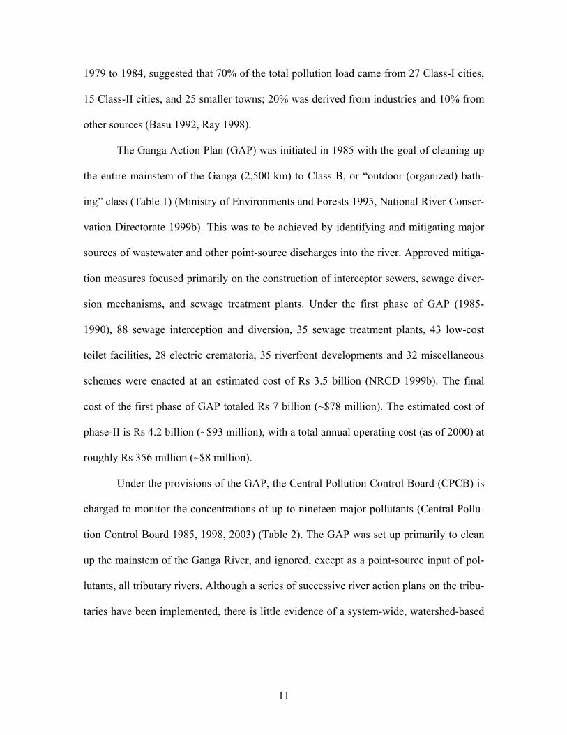
The Ganga Action Plan (GAP) was initiated in 1985 with the goal of cleaning up

the entire mainstem of the Ganga (2,500 km) to Class B, or “outdoor (organized) bath-

ing” class (Table 1) (Ministry of Environments and Forests 1995, National River Conser-

vation Directorate 1999b). This was to be achieved by identifying and mitigating major

sources of wastewater and other point-source discharges into the river. Approved mitiga-

tion measures focused primarily on the construction of interceptor sewers, sewage diver-

sion mechanisms, and sewage treatment plants. Under the first phase of GAP (1985-

1990), 88 sewage interception and diversion, 35 sewage treatment plants, 43 low-cost

toilet facilities, 28 electric crematoria, 35 riverfront developments and 32 miscellaneous

schemes were enacted at an estimated cost of Rs 3.5 billion (NRCD 1999b). The final

cost of the first phase of GAP totaled Rs 7 billion (~$78 million). The estimated cost of

phase-II is Rs 4.2 billion (~$93 million), with a total annual operating cost (as of 2000) at

roughly Rs 356 million (~$8 million).

Under the provisions of the GAP, the Central Pollution Control Board (CPCB) is

charged to monitor the concentrations of up to nineteen major pollutants (Central Pollu-

tion Control Board 1985, 1998, 2003) (Table 2). The GAP was set up primarily to clean

up the mainstem of the Ganga River, and ignored, except as a point-source input of pol-

lutants, all tributary rivers. Although a series of successive river action plans on the tribu-

taries have been implemented, there is little evidence of a system-wide, watershed-based

12

management strategy in the Ganga watershed (Iyer 2003, Alley, personal communica-

tion).

The government of India states that the GAP has improved water quality of the

river. It bases this assertion on changes in monitored water pollution concentrations

(NCRD 1999a), but gives no data on seasonal estimates or loading estimates. Most previ-

ous analyses of the GAP have focused on the economic impacts of the plan (Markandya

& Murty 2000), or certain river reaches between major cities (Ray 1998, Krishna Murti

1995, Tare et al 2003). As of 2005, there has not been a publicly-available comprehen-

sive assessment of the impact of the GAP on the water quality in the Ganga watershed.

The question of how successful the GAP has been is an important and timely one.

The GAP was initiated in 1984, just over twenty years ago. During the interim, the GAP

stimulated many governmental reforms relating to the river, both positive and negative.

In recent years, many NGOs and news organizations regularly assert that that the GAP

has failed, and concerns about the future of the Ganga continue to be raised (Tare et al

2003, Alley, 2002).

In this report, I review the efficacy of the GAP and provide an overview of the

current state of water quality in the Ganga basin through the development of empirical

flow and pollutant loading models. This study attempts a preliminary answer to the ques-

tion, “After twenty years, did the Ganga Action Plan bring about positive water quality

change to the Ganga watershed?” Using publicly-available historic water quality and wa-

ter quantity data, supported by my own observations during a field sampling trip in Janu-

ary and February 2004, I have developed several different analyses of the efficacy of the

GAP. As discussed below, my analysis indicated that the GAP did, in fact, improve

13

mainstem waster quality of some parameters, but also raises questions about the sustain-

ability of current levels of water pollution in the Ganga basin.

14

Methods

In order to analyze GAP performance using CPCB data, it was necessary to first

construct a basin-wide hydrologic model for annual average flows. This hydrologic

model was necessary because flow and discharge data were classified as confidential ma-

terial in 1974 (coincident with the completion of the Farakka Barrage), and have not been

declassified since (Iyer, personal communication). The constructed hydrologic model es-

timated pollutant loading rates from CPCB-reported annual average pollutant concentra-

tions. The results from the hydrologic model were used to develop a simple empirical

pollutant loading model for each CPCB subwatershed unit as a part of my evaluation of

the current status of Ganga River waters. They were also used to statistically evaluate the

historical effectiveness of the GAP. I also developed a second pollution prediction model

based on total per capita loading rates used in environmental engineering.

In addition to CPCB water quality data, I collected water samples during January

and February 2004 at six different Indian cities that were analyzed for the standard pol-

lutants of nitrate, phosphate, COD, and ammonia.

Construction of an annual average discharge (Q) model

There is a strong logarithmic relationship between drainage area and average ba-

sin hydraulic parameters, including discharge, generally described as the hydraulic ge-

ometry (Leopold 1997). Taking advantage of this relationship, a regression model was

constructed for annual average discharge in the Ganga basin as a function of tributary wa-

tershed area using data average annual flows for 1963-1973 (Rao 1975) (Table 3). Up-

stream watershed areas of CPCB sampling points on were estimated using ArcMap, ver-

sion 9.1 (ESRI 2005).

15

Because I would need to extrapolate to smaller and larger subbasins than provided

by the available Ganga hydrographic data, I used an Analysis of Covariance (ANCOVA)

to test slope and intercept of the Ganga’s derived linear regression equation against a

similar linear regression equation I produced of major and minor world rivers which

spanned a greater range of basin sizes. (Figure 6). No significant difference was found in

either slope or intercept between the regression equations of the Ganga River and other

world rivers (Table 4, Table 5). On the basis of these analyses, I concluded it was reason-

able to extrapolate from the available range of data making up the Ganga linear regres-

sion discharge model to larger and smaller basins within the Ganga system.

The Himalaya Mountains contain vast glaciers, the melting of which provides

60% of the water in the Ganga Basin (Ray 1998). Because this significant input to the

Ganga is known, the Himalayan mountain range was delineated, and the percentage of

each subwatershed in the Himalayan Mountains (% Himalaya) has been incorporated into

the model. The percentage of a subwatershed in the southerly Vindhya Mountains proved

to be a non-significant model parameter, and was not used. Similarly, since the yearly

monsoon was known to have significant impacts on river discharge (Figure 4), each sub-

watershed’s average yearly precipitation has been incorporated into the model. Although

several major canal projects exist within the Ganga Basin, some removing up to 325 m3/s

(cms) from the river (Ray 1998), these removals were not included in the model due to

lack of accurate spatial data. Effects of dams and other major water projects were not in-

cluded in the model for the same reason. The final multiple linear regression model used

total subwatershed basin area (A), annual precipitation within the subwatershed (P), and

16

the percentage of the subwatershed in the Himalaya mountains (% Himalaya) to predict

annual discharge (Table 9).

( ) ( )( ) ( )( ) ( )( ) 698.4001.1%Himalaya0.001P0.846AlnQln −++= (R2=95.5%)

EQUATION 1 This model overestimated flows by 10.2% on average (-30.2% to 60.8%). Water-

sheds originating in the Himalayas were over-estimated by roughly 11.8%. Modeled dis-

charge values of the Ganga at Allahabad before the Sangam were under-predicted by

29.5% the reported value. The Gandak, Sone, and Ghaghara rivers were all under-

represented by 30.2%, 23.0%, and 22.2%, respectively. The Bhuri Gandak was greatly

over-represented by 60.8%. The Kosi was over-represented in the model by 20.6% and

the Tons by 20.5%. The only non-Himalayan river that was greatly divergent from its es-

timated value was the Gomati, the model yielding a discharge of 44.7% above the re-

ported value of 209 cms (Table 7).

These regression analyses and all other statistical methods employed in this study,

apart from the ANCOVA tests, were performed using Data Desk, version 6.1 (Data De-

scription 1996). The ANCOVA tests were calculated by hand.

Central Pollution Control Board Data

The CPCB water quality monitoring sites were acquired from published Water

Quality Yearbooks (CPCB 1985, 1998, 2003). The location of each city was found by

using a variety of paper (US Army Map Service 1955) and online (National Imagery and

Mapping Agency 1998, Google 2005) maps to determine the longitude and latitude of

each site. 104 of the 156 reported sampling sites were located. When a city had more than

17

one site associated with it, with no additional information other than “upstream” and

“downstream,” a distance of roughly 20 kilometers was used to separate sites.

Watershed boundaries for each CPCB water quality sampling station were deline-

ated using the watercrsl and inwatera shapefile layers from the “vector map level 0”

(VMAP-0)6 data sets (NIMA 1998). Publicly-available VMAP-1 layers included only the

western Ganga Basin, and were therefore not used. The area of each watershed was de-

termined using the analysis tools in ArcMap 9.1 (ESRI, 2005). No significant difference

was observed between derived tributary watershed areas delineated in this process and

the values cited by Rao (1975) (Table 8).

Using the constructed multiple linear regression discharge model (Equation 1),

average annual loads were calculated for each chemical component at each CPCB station.

Values for total dissolved solids (TDS) were not available pre-GAP. Based on sites where

TDS and conductivity were available post-GAP, values for TDS were calculated based

on the regression-calculated conversion factor of 59.1tyconductiviTDS = (y = 0.6305x, R2=

0.3704, n= 52). Total nitrogen was calculated by summing NOx and TKN values for each

site.7

All available CPCB annual average pollutant values pre-GAP implementation

(1980-1984) were averaged at each site to obtain a grand mean. Similarly, data values for

1998 and 2003 were averaged at each site to obtain mean post-GAP pollutant values.

6 VMAP-0 level data has a spatial resolution of 1:1,000,000, covers the entire world, and is publicly avail-able for download from various websites. The world is divided into four regions, North America (NO-AMER), Europe and North Asia (EURNASIA), South America, Africa, and Antarctica (SOAMAFR), and South Asia and Australia (SASAUS). 7 Loads values for total coliforms, fecal coliforms, dissolved oxygen, temperature, and pH are nonsensical measures, and were not calculated.

18

Most pollutant load values were found to be right-skewed, and were normalized

using a log-transformation. Changes in water quality were analyzed using paired, two-

tailed, t-tests and compared “pre-GAP” and “post-GAP” pollutant levels to determine the

GAP policy in monitored regions of the Ganga River basin.

Construction of the Ecological Valley Segment Model

Large portions of the Ganga watershed, mostly in Nepal and less-populous re-

gions of the watershed were not monitored by the CPCB (Figure 7). In order to obtain

pollution estimates for these regions, it was necessary to delineate regions within which

extrapolations could be made based on available CPCB data.

A preliminary ecological valley segment (VSEC) model (Seelbach & Wiley,

2005) was created for the Ganga by delineating segments based on watershed boundaries

and river planform. A more complete model could have been based on land cover/land

use, ground water flux, inputs from secondarily-significant tributaries, major water ab-

stractions, impoundments, etc. However publicly-available, land cover data was scarce,

not uniformly representative of the watershed, and usually out-of-date. A recently-created

land use layer of the Indus and Ganga river basins, described by Thenkabail, et al (2005)

may be useful for future revisions.

The VSEC classifies the river into ecologically-homogenous reach units. Signifi-

cant changes in land cover, ground water flux, surficial geology, river discharge, etc. in-

dicates potential significant changes in river inputs and lead to new ecological conforma-

tion in the channel (Seelbach et al 1997). A comprehensive valley segment classification

provides useful units for extrapolation and regional modeling efforts (Seelbach & Wiley

2005).

19

River planform8 was used as a primary means of characterizing changes in valley

segment character, since the measurement of sinuosity is correlated with the type of

surficial geology, average annual discharge, and slope of a river (Leopold 1997). Map-

ping of VSEC units was based on the publicly-available waterscrsl and inwatera shape-

files (National Imagery and Mapping Agency 1998) used in deriving river discharge.

Estimating Pollution Beyond CPCB Basins

The CPCB water quality monitoring focused primarily upon population centers

within the Ganga River watershed. However, not all major cities’ water quality data were

reported, one obvious omission being Patna, the capital city of Bihar, with an estimated

population of 1.3 million people in 2000 (Census of India 2000). Furthermore, the lack of

water quality information from most major tributary streams of the Ganga makes it diffi-

cult to conduct a basin-wide review of water quality. Two methods were used to estimate

pollutant loading across the Ganga watershed: a potential loads-based model on average

per capita pollutant loading estimates, and the multiple linear regression model based on

observed patterns of pollutant loading. Estimates were only made for the period of time

contemporary to the “Post-GAP” (1998, 2003), because population data during the “Pre-

GAP” period were not available at a finer resolution scale than the administrative district

level.

Empirical Pollutant Loading Estimates

Multiple linear regression (MLR) models of average annual BOD5 (Table 10),

total nitrogen (Table 11), and TDS (Table 12) pollutant loading (mg/s) were created

based on recent observed average CPCB values (1998 and 2003). Regression analyses of

8 The river’s planform is its shape as viewed from above, or on a map.

20

estimate pollutant loads were based on the parameters of upstream subbasin area, dis-

charge, and regional population9, and produced the following equations:

ln(BOD5) = -0.542 + ln(Qcms)(0.320) + ln(Pop’nwatershed)(0.435) (R2=73.4%) EQUATION 2

ln(Ntotal) = -3.553 + ln(Qcms)(0.067) + ln(Pop’nwatershed)(0.724) (R2=67.9%)

EQUATION 3 ln(ColiformsTotal) = -5.725 + ln(Qcms)(-1.515) + ln(Pop’nwatershed)(1.677) (R2=30.7%)

EQUATION 4 ln(TDS) = 1.231 + ln(Qcms)(0.212) + ln(Pop’nwatershed)(0.698) (R2=69.4%)

EQUATION 5 ln(Calciumtotal) = -0.893 + ln(Areawatershed)(0.583) + ln(Pop’nwatershed)(0.342) (R2=94.8%) EQUATION 6 ln(Chloride) = -2.29183 + ln(Pop’nwatershed)(0.806) (R2=100%) EQUATION 7 The modeled values of each parameter were calculated with each VSEC basin in

order to gain a better understanding of the potential current state of water quality in re-

gions that fall outside the purview of the CPCB’s monitoring programs. Using a slightly

modified classification (Table 16), each VSEC unit was then categorized into CPCB wa-

ter quality codes.

Per capita Potential Loads

It is possible to estimate the maximum BOD5, total nitrogen, and total phosphate

loading in a basin based on standardized values for municipal sewage. The maximum ex-

pected impacts of the estimated upstream population within a 50 km radius of each VSEC

node was calculated to help estimate phosphate loads.

9 Population at 100km radius upstream from the subbasin discharge point.

21

Following Schwoerbel (1987), I estimated the maximum potential daily inputs of

BOD5, nitrogen, and phosphate as:

( ) ( )( )( )15total5 y/person/daBOD kg00135.0PopulationBOD cload = Equation 8

( ) ( )( )( )2total ayN/person/d kg00225.0PopulationN cload = Equation 9

( ) ( )( )( )3450km4 y/person/daPO kg0015.0PopulationPO cload = Equation 10

where ci is the respective delivery ratio of the pollutant to the river10. Knowing that the

MLR-based pollutant loading values of BOD and nitrogen indicate post-GAP loading

rates, it was possible to estimate the average pollution treatment levels at each VSEC, and

thereby obtain the values for c1 and c2 by regressing the maximum potential daily pollut-

ant input against the MLR loading estimate from above. The value of the slope coeffi-

cient of the maximum potential daily loading was used as the estimated dimension of ci.

This gave estimated ci values of BOD5 and N of 0.734179 and 0.285403, respectively.

The estimated delivery ratio of phosphate was arbitrarily set at c3 = 0.6; a delivery ratio

that assumes processing equivalent to full secondary treatment.

Pollution Analysis

Using the pollution estimates obtained from the empirical pollutant loading MLR

models, and the modeled river discharges, pollutant concentrations of Total Coliforms11,

BOD5, and conductivity were calculated for VSEC segment12. A modified version (Table

16) of the CPCB criteria for assessing water quality was used to assign the water quality

of each segment based on individual pollutants. Then, the overall water quality class was

10 ci= kg of pollutant/day 11 Although the total coliform parameter had only a 30.7% R2 value, it was extrapolated across the basin because it is a vital component of the CPCB’s water quality classification scheme. 12 Conductivity was calculated as TDS*1.59=conductivity.

22

determined by assigning the maximum criteria standard. For example, if a VSEC segment

was rated a class A for conductivity, but a class D because of total coliform counts, that

segment was assigned an overall class of D.

Sampling in India

In January and February 2004, I collected water samples were collected in India

along the Ganga at the cities of Hardwar13, Kanpur, Allahabad14, Varanasi15, Patna16, and

Kolkata17 (Figure 9). Collected water samples were tested at each site for ammonia (NH4),

total soluble phosphate (TSP), nitrate/nitrite (NO3-N), and COD content. COD values ex-

ceeded what could be measured with the reagents available onsite, so a lower-bound of

COD was calculated for each site. Load estimates were not calculated, because daily flow

values were not publicly available for these sites.

Sampling Sites

Hardwar: Sampling in Hardwar took place above the city and the canal headworks

of the Upper Ganga Canal, at the site of the large statue of Shiva (Figure 10) This site is

situated immediately of a dam that was constructed to divert water to run either through

the city of Hardwar and into the Upper Ganga Canal, or along the original course of the

Ganga. The Ardh Kumbh Mela18 was just starting at Hardwar, and areas in and just below

13 Also known as Haridwar. 14 Also known as Prayag. ‘Prayag’ is rarely used outside a Hindu religious context. 15 Also known as Varanassi, Benares, Banares, and Banaras. 16 Also known as Pataliputri. Although many city and place names have been reverted from their British transliterations of the local Hindi, ‘Patna’ is preferred over the historical ‘Pataliputri.’ 17 Also known as Calcutta. 18 The Ardh Kumbh Mela is a Hindu pilgrimage held once every twelve years, and compliments the more popularly-attended Kumbh Mela pilgrimage. During the Ardh Kumbh Mela, Hindu pilgrims travel to holy sites in the cities of Hardwar and Allahabad. The city of Hardwar may have up to 1 million pilgrims over the course of one month. The city of Allahabad, being both easily reached, and a more holy city, can have up to 50 million pilgrims over the course of the same month.

23

the city was already closed off for the exclusive use of pilgrims, limiting the choice of

sampling sites.

Kanpur: Two sites were sampled in Kanpur (Figure 11). The first site was at one of

the municipal water intake points for the city. The pumping station was built in the mid-

1960s on the banks of the Ganga, but during the intervening 40 years, the river has

shifted its course to the north and east by six kilometers. The site gets its water from two

feeder canals that lead from the Ganga. Slum development has taken place along both

banks of the canals (Figure 12). The second site was on the Ganga itself, downstream

from Kolya Ghat; near the eastern end of the city, but upstream of the major industrial

tanneries (Figure 13).

Allahabad: Two sites were sampled in Allahabad (Figure 14). The first site was 2

kilometers below the Sangam, river right (Figure 15). The majority of the flow at this

point, from the Yamuna River, converges from the west and south of the Ganga. The sec-

ond site was above the Sangam (confluence of the Ganga and Yamuna Rivers), on the

Ganga, below two rail bridges and a road bridge (Figure 16). Sampling in Allahabad was

made difficult by the ongoing Ardh Kumbh Mela pilgrimage and celebrations taking

place at the Sangam itself.

Varanasi: Sampling was done at one site, opposite of Asi Ghat, at the downstream

end of the city’s pilgrimage area (Figure 17). The city of Varanasi is a major pilgrimage

city, and although not one of the Ardh Kumbh Mela pilgrimage cities, does have a large

number of pilgrims arriving every day. However, this sampling site, located in the middle

of the river, should not have been affected by the pilgrims and religious rituals taking

24

place along the ghats because of the low level of mixing between river edge and midriver

(Figure 18).

Patna: Sampling in Patna was done downstream of the confluence with the Gan-

dak and Bhuri Gandak Rivers (Figure 19, Figure 20). Upstream of this sampling site, the

Ganga is intercepted by the Ghaghara and Gandak from the north and the Sone from the

south. None of these major tributaries have any cities of over 1 million people directly

along their banks.

Kolkata: Sampling in Kolkata was conducted on the Hooghly River19, just outside

that grounds of the Botanical Gardens (Figure 21). Samples were collected during the pe-

riod of the rising tide, and the river was moving south-to-north. Sampling, during the fal-

ling tide was not done, due to safety concerns.

19 Also known as the Bhagirathi or Hugli River, the Hooghly River one of the major distributaries of the Ganga River. The majority of water entering the Hooghly is diverted south from the Farakka Barrage, 18km upstream from the border with Bangladesh to maintain the deep water port of Kolkata (Adel 2001).

25

Results

Pre-Post GAP Comparisons

Water quality reported by the Central Pollution Control Board before the imple-

mentation of the Ganga Action Plan was poor, with DO as low as 0.1 mg/L (mean: 7.4

mg/L), BOD as high as 175 mg/L (mean: 5 mg/L), COD at 770 mg/L (mean: 27 mg/L),

NOx at 80 mg/L (mean: 5.9 mg/L), pH ranging from 1.5 to 13.8 (mean: 8.0), fecal coli-

form levels of 2.4 x 108 MPN/100 mL (mean: 2.2 x 105 MPN/100 mL), total coliform

levels of 2.4 x 108 MPN/100 mL (mean: 2.5 x 105 MPN/100 mL), conductivity of 20,000

mg/L (mean: 449 mg/L), chloride at 3234 mg/L (mean: 38 mg/L), sulfate at 2100 mg/L

(mean: 29 mg/L), sodium at 16200 mg/L (mean: 32.9 mg/L), calcium at 340 mg/L (mean:

78.3 mg/L), and magnesium at 995 mg/L (mean: 49.2 mg/L). After roughly twenty years

of GAP implementation, DO levels were as low as 0.3 (mean: 7.3 mg/L), BOD as high as

230 mg/L (mean: 6.6 mg/L), COD at 999.9 mg/L (mean: 36.5 mg/L), NOx at 3.5 mg/L

(0.1 mg/L), pH ranging from 2.0 to 10.0 (mean: 7.9), fecal coliform levels of 1.9 x 1010

MPN/100 mL (mean: 2.3 x 107 MPN/100 mL), total coliform levels of 9.5 x 109

MPN/100 mL (mean: 9.2 x 106 MPN/100 mL), conductivity of 11,660 mg/L (mean:

514.9 mg/L), chloride at 4674 mg/L (mean: 83 mg/L), sulfate at 9999 mg/L (mean: 157.3

mg/L), sodium at 1328 mg/L (mean: 83.4 mg/L), calcium at 1140 mg/L (mean: 122

mg/L), and magnesium at 1330 mg/L (mean: 75.5 mg/L) (Table 17).

While overall basin means of most measured Ganga water quality parameters did

not significantly differ before and after GAP, a paired t-test comparison of the pre- and

post-GAP samples by sampling location showed that accounting for site to site variation,

the water quality in the Ganga River had significantly improved (preGAP – postGAP >

26

0) for some important parameters. Improving water quality parameters included BOD (t:

1.904, p: 0.0323), dissolved oxygen (t: -1.515, p: 0.0690), and nitrogen (t: 5.209, p:

0.0004) concentrations. However, several factors indicated a decline in quality after

twenty years of GAP (preGAP – postGAP < 0), including Fecal Coliform count (t: -1.439,

p: 0.0793), Total Coliform count (t: -1.321, p: 0.0974), and concentrations of calcium (t: -

1.578, p: 0.0639), magnesium (t: -1.968, p: 0.0304), and TDS (t: -2.139, p: 0.0195). Dif-

ferences between pre- and post-GAP levels of COD, pH, temperature, alkalinity, chloride,

sulfates, and sodium were not statistically significant (Table 18).

Indian Field Data

The water samples from my January/February 2004 trip revealed that during that

period, water quality was highest at Hardwar and Patna, and lowest near Kanpur, and at

Allahabad, below the Sangam. (Table 19).

At Hardwar, both ammonia and phosphate were below detection levels, and level

of NOx (0.02 mg/L) was the lowest observed among all the sampling locations. Kanpur’s

water intake site had the highest ammonia level (2.75 mg/L), and the second highest

phosphate concentration (1.26 mg/L) among all sampling locations. The site opposite

Kanpur’s Kolya Ghat had the highest phosphate (6.2 mg/L) and NOx (0.74 mg/L) con-

centrations among all sites. Allahabad above the Sangam had relatively very low concen-

trations of ammonia (0.02 mg/L) and phosphates (0.03 mg/L), and a slightly-above-

median concentration of NOx (0.29 mg/L). Below the Sangam (and past the thousands of

pilgrims bathing at the confluence point), increased concentrations of ammonia (0.20

mg/L), phosphate (0.29 mg/L), and NOx (0.39mg/L) were observed. At Varanasi, ammo-

nia (0.22 mg/L) and NOx (0.20 mg/L) were similar to Allahabad below the Sangam. The

27

phosphate concentration was relatively low (0.04 mg/L), but still elevated by natural

standards. At Patna, ammonia was not detected. Phosphate was elevated (0.13 mg/L) but

NOx (0.09 mg/L) were relatively low. Kolkata had a relatively low level of NOx (0.12

mg/L), elevated ammonia (0.54 mg/L) and very high levels of phosphate (2.95 mg/L).

Estimated water quality using empirical loading models

The empirical load models (Equation 2, Equation 3, Equation 4, Equation 5) and

estimated average annual flows (Equation 1) were used to estimate BOD, nitrogen, and

TDS for all of the delimited VSEC units in the Ganga Basin (Table 20). BOD loading

estimates ranged from 9.04 kg/day to 4097.52 kg/day (median: 198.41 kg/day, mean: 430

kg/day), with BOD concentrations ranging from 1.18 mg/l to 42.68 mg/l (median: 9.75

mg/l, mean 10.27 mg/l). Nitrogen loading estimates ranged from 2.16 kg/day to 757.78

kg/day (median: 89.16 kg/day, mean: 139.12 kg/day), and nitrogen concentrations ranged

from 0.11 mg/l to 49.79 mg/l (median: 3.70 mg/l, mean 6.43 mg/l). TDS loading esti-

mates ranged from 366.37 kg/day to 1,417,185.22 kg/day (median: 36,275.81 kg/day,

mean: 112,882 kg/day), and TDS concentrations ranged from 60.13 mg/l to 5,498.66

mg/l (median: 1,850.92 mg/l, mean: 1,918.04 mg/l). Chloride loading estimates ranged

from 12.16 kg/day to 47,713.23 kg/day (median: 1,563.07 kg/day, mean: 4,544.35

kg/day), and chloride concentrations ranged from 1.66 mg/l to 435.52 mg/l (median:

84.88 mg/l, mean: 97.57 mg/l). Calcium loading estimates ranged from 62.49 kg/day to

75,948.38 kg/day (median: 1,852.59 kg/day, mean: 5,975.65 kg/day) and calcium con-

centrations ranged from 10.27 mg/l to 209.5 mg/l (median: 95.34 mg/l, mean: 94.61 mg/l).

Total coliform concentrations ranged from 20.97 MPN/100 mL to 860,949.03 MPN/100

mL (median: 90,650 MPN/100 mL, mean: 187,163.62 MPN/100 mL).

28

Per capita Potential Loads

The per capita potential loads model was able to give estimates of BOD, total ni-

trogen, and phosphate throughout all the VSEC basins (Table 21). BOD loading estimates

ranged from 0.91 kg/day to 26,226 kg/day (median: 377.34 kg/day, mean: 1,875.34

kg/day). BOD concentrations ranged from 0.01 mg/l to 7.75 mg/l (median: 1.92 mg/l,

mean: 2.30 mg/l). Nitrogen loading estimates ranged from 5.91 kg/day to 169,922 kg/day

(median: 2,444.80 kg/day, mean: 12,150.27 kg/day), and nitrogen concentrations ranged

from 0.09 mg/l to 50.21 mg/l (median: 12.44 mg/l, mean: 14.87 mg/l). Phosphate loading

estimates ranged from 0.17 kg/day to 387.22 kg/day (median: 18.74 kg/day, mean: 30.94

kg/day), and phosphate concentrations ranged from effectively 0 mg/l to 2.30 mg/l (me-

dian: 0.07 mg/l, mean: 0.17 mg/l).

Based on the per capita phosphate model predictions, concentrations of phosphate

were more dilute as the total discharge in the river increased (Figure 28). The highest

concentrations are seen in the Gomati River, the Tons river, and the Yamuna river above

the confluence with the Chambal River. This is expected because the populations of the

regions are very high, including the cities of Delhi (14.1 million), Chandigarh (9 million),

Gwalior , and Lucknow (2.3 million) (Census of India, 2001). These estimates are likely

understating the actual average annual concentrations of PO4, since agriculture is very

prolific throughout the Ganga Basin, even into the foothills of the Himalayas.

The modeled phosphate values at Hardwar, Allahabad (above Sangam), and Va-

ranasi were all within 0.05 mg/L of the observed field values. The measured values at

Kanpur (Kolya Ghat), Allahabad (below Sangam), and Patna were all markedly higher

than the modeled values. The values measured in Kanpur (6.2 mg/L) exceeded the mod-

eled value of the VSEC river segment by roughly 6 mg/L. Part of this is likely due to a

29

modeling error, since the VSEC unit including Kanpur terminated further than 50 km

downstream of the city (Figure 34). For this reason, this VSEC unit did not include the

city in the analysis. However, even if the city’s estimated population of 2.9 million (Cen-

sus of India 2001) had been included in the calculation, the estimated annual average

concentration would be 0.32 mg/L, far lower than measured. Similarly, the estimated

phosphate levels at Allahabad (below Sangam) (0.29 mg/L) and Patna (0.13 mg/L) are

both much lower than measured in 2004.

Estimate Comparisons

The two basin-wide pollution estimation methods provided different values for

each site (Table 22). The MLR estimates for nitrogen loading and concentrations were on

average 76.25 times greater (stdev=79.58) than the per capita estimates. The estimates

ratio for BOD5 were closer to each other, but the MLR estimates were on average 12.76

times greater (stdev=19.90) then the per capita estimates. Comparisons for total coliforms,

chlorine, calcium, and TDS were not done, as there was no available per capita equation

estimate for these pollutants. Conversely, a comparison for phosphate was not done, as

there was no available empirical data available.

VSEC Basin Water Quality Classes

Using the empirical loading models, water quality classes were derived for each

VSEC basin. Classification of water quality classes A, B, and C were assigned based on

values of BOD and total coliforms. Estimates of BOD indicated that 658 river miles

(1,059 km) were class A, 624 river miles (1,004 km) were class B, 168 river miles were

class C, and the remaining 7281 river miles (11,717 km) exceeded class C BOD require-

ments (Figure 29). Based on total coliform estimates, 129 river miles (208 km) were class

30

A, 776 river miles (1,249 km) were class B, and 359 river miles (578 km) were class C.

The remaining 7,467 river miles (12,017 km) exceeded class C total coliform require-

ments (Figure 30).

Of the 7,467 river miles (12,017 km) that exceeded class C requirements of total

coliform counts or BOD concentration, 983 river miles (1,582 km) met the class D re-

quirement of nitrogen (Figure 31). Of the remaining 6,484 river miles (10,485 km), 1,236

river miles (1,989 km) met the class E conductivity requirement, leaving 5,249 (8,447

km) river miles as being worse than class E (Figure 32).

Combining the water classification results, 5,249 river miles (8,447 km) were

worse than class E, 1,236 river miles (1,989 km) were class E, 983 river miles (1,582 km)

were class D, 425 river miles (684 km) were class C, 710 river miles (1,143 km) were

class B, and 129 river miles (208 km) were class A (Figure 33). In the Ganga River main-

stem, 129 river miles (208 km) were class A, 103 river miles (166 km) were class B, 81

river miles (130 km) were class C, 466 river miles (750 km) were class D, and 654 river

miles (1,053 km) were worse than class E. Himalayan rivers (excluding the Ganga) gen-

erally had higher water qualities than non-Himalayan rivers, with 608 class B river miles

(975 km), 344 class C river miles (554 km), 517 class D river miles (832 km), 827 class

E river miles (1,331 km), and 1,237 river miles (1,991 km) that were worse than class E.

Non-Himalayan rivers had no class A, B, C or D waters, 409 river miles (658 km) of

class E, and 3,358 river miles (5,404 km) that were worse than class E (Table 19).

31

Discussion.

GAP evaluation

Based on the pre-GAP vs. post-GAP statistical analysis, it appeared that the key

factors of DO, BOD, and nitrogen improved since the implementation of the Ganga Ac-

tion Plan. These average annual declines in concentrations indicate that, overall, envi-

ronmental conditions in the river have improved vis-à-vis the chemical components of

domestic sewage. In this sense, a portion of the primary goal – reaching class B or better

(MoEF, 2004) – of the GAP appears to be working.

However, total coliforms and fecal coliform levels appear to have deteriorated in

the same period. This is most likely the direct impact of population growth without a

commensurate increase in the region’s pollution management infrastructure. Indeed, the

story of much of the water infrastructure in the Ganga basin is one of bad planning, ne-

glect, and failure (Niemzcynowicz et al 1998, MoEF 2004). Since total coliform counts

are a central part of classifying a water’s quality as class C or better (Table 1), unless

coliform counts are greatly diminished, the water quality goals of the GAP will not be

reached.

Implications of Increased Fecal Coliform Levels

The increased levels of total coliforms post-GAP was the major reason why so

many sites did not achieved even class C status20. The associated increased levels of fecal

coliform levels point to a looming public health crisis caused by a inexorable loss and

pollution of existing water sources, which is only exacerbated by an ever-increasing poor

population (Niemczynowizc et al 1998). Water development post-independence focused 20 Classes A, B, and C all have a total coliform requirement. Classes D, and E do not have this requirement.

32

primarily on agriculture and industry, and India has still not been able to provide safe,

potable drinking water to its populace through public infrastructure (Chaturvedi 2001).

People living in cities and towns in the Ganga basin that receive their water directly from

the Ganga suffer many enteric diseases (Gourdji et al 2005). In 1955 and 1956, 40,000

Delhi residents fell victim to infective hepatitis contracted from drinking water from the

Yamuna River, and an estimated 50-75% of the human population of India’s major cities

suffers from several stomach ailments and digestive diseases (Maruthanayagam & Kumar

2002). Pandey (1991) also made a connection between elevated coliform counts down-

stream of Kanpur and increased enteric diseases of local villagers who used water drawn

from the river. During a visit to a health clinic in Hardwar in January 2004, doctors were

expecting to have several thousand patients complaining of gastrointestinal disease.

One possible major source of such high levels of fecal coliforms is public defeca-

tion, which is common in many places in northern India, and personally witnessed in all

the cities visited. Part of this is a lack of public restrooms, or a lack of sanitary public

restrooms, where such are constructed. Krishnan & Sujatha (2002) reported public defe-

cation rates of 18.4 ± 0.83 visits/½ hour on the banks of an urban river in southern India.

Rates upstream and downstream of the city were lower. Interestingly, public defecation

rates increased during the monsoon. This increase was hypothesized to be due to the in-

creased accessibility to water. Added to defecation levels of a city’s human occupants is

the defecation rate of the animals, which may be found roaming the streets, or freely ac-

cessing the river.

Presence of fecal coliforms indicates a lack of proper sewage treatment. In re-

gions where fecal coliforms are high, other bacteria or intestinal parasites may also be

33

found in the water, posing additional health risks to bathers. Indirect contraction of these

parasites through eating fish – a major source of protein – that are infected is also possi-

ble (UNESCO 2006).

Part of the solution is the construction and maintenance of public toilet facilities

to decrease the amount of unsewered fecal discharge. Without these facilities, construc-

tion of additional sewage treatment plants is not useful. However, in many areas, the con-

struction and maintenance of, and assured power for sewage treatment plants is still re-

quired (MoEF, 2004). A short- to medium-term solution of lower cost may be the con-

struction and encouraged use of pit latrines (UNESCO 2006), especially in areas with lit-

tle or no effective sewage infrastructure.

Changing the Criteria

An interesting point to mention was the one-year change of water quality criteria

that occurred in 2002. Although there is no indication as per motive, the CPCB adopted a

“Revised Water Quality Criteria” (Table 24), splitting the existing six water quality

classes (A-E, worse than E) to three classes (A-C) (CPCB, 2002). The 2002 classification

system was, while having a greater number of parameters, less stringent in terms of con-

ductivity and BOD than the original, and none of the new classes include those of ex-

tremely poor water quality as the original classes D and E. Whether this was an attempt at

changing the standard to accommodate reality (and thereby proclaim success), or an at-

tempt at conducting a systematic change unrelated to water quality goals is not clear; no

explanation is available for the changes.

34

On a quick assessment of the 2002 data, 9 sites (8.7%) were class A, 43 sites

(41.7%) were class B, and 51 sites (49.5%) were class C21. With the revised criteria, over

half of the monitored sites were “in attainment” of the Ganga Action Plan. In 2003, the

CPCB reverted to the original water quality criteria. The reasons why they reverted to

their original criteria remain unexplained. The reported water quality data for 2002 re-

main as nominal categories (A, B, and C), rather than the otherwise-normal array of

minimum, maximum, and mean observations. Using the original classification system

with the 2003 data, there were no sites achieving class A, 11 sites (9.7%) were class B,

29 sites (25.7%) were class C, 19 sites (16.8%) were class D, 46 sites (40.7%) were class

E and 8 sites (7.1%) were worse than class E (Table 25).

Although there is no evidence for why the CPCB returned to the original water

quality classification system, the discrepancy between the range of water quality reported

under the “Revised Water Quality Criteria” and the original criteria may have provoked a

public outcry, especially if the CPCB used the new criteria to show a greater number of

sites achieving class B status.

Current water quality on Ganga

Based on the CPCB’s original water quality criteria, the majority of the river is in

poor shape; even in regions of the watershed that are not monitored by the CPCB. With

near consistency, it would appear that the GAP has failed to effectively return the Ganga

River to bathing (B) class. Furthermore, based on the model output, the CPCB should

focus their monitoring and enforcement efforts within the southern tributary systems, the

Gomati River watershed, the upper half of the Yamuna River, and the parallel portion of

21 2002 data from the CPCB were given in A, B, and C classes.

35

the Ganga River. These, coincidently, are regions of low flow and high population den-

sity.

The modeled phosphate concentrations indicate the additional need for the CPCB

to monitor and control phosphate levels. The model does not include any possible inputs

from agriculture, but with phosphate inputs from pesticides and fertilizers, the actual lev-

els can be much higher than modeled (see below).

Variation of phosphate between modeled and measured values

The highly-divergent observed phosphate value found at Kanpur (Kolya Ghat)

may have been due to several factors. The first factor was the non-inclusion of Kanpur’s

population within the VSEC arc’s watershed, as mentioned earlier. However, even if the

city’s population were included, it would not approach the observed value of 6.2 mg/L.

Two observed phenomena at Kanpur were untreated sewage and a vast amount of flood-

plain agriculture. In addition to the possibility of agricultural phosphate, Panday (1991)

lists six different pollution sources at Kanpur, including 16 untreated sewers, dead bodies,

dairies housing over 80,000 milk cows, night soil disposal, and 160 tanneries. There is,

unfortunately, no published value of the amount of phosphate fertilizers used in and

around the city, nor a baseline phosphate value against which to base the measured result.

If a majority of the sewage in Kanpur is not treated, and phosphates are used extensively

in regional agriculture, these will have a major impact on the observed phosphate levels

in the river, as the discharge of the Ganga River is relatively smaller than at other meas-

ured sites.

The major impacts to the phosphate values at Allahabad (below Sangam) may

have been due to two phenomena: the Ardh Kumbh Mela pilgrimage, and primary sew-

36

age discharge into the Yamuna River. The sampling day in Allahabad was also republic

Day, a national holiday, and the shores of the Yamuna-Ganga confluence were full to ca-

pacity with people. In addition, there were seemingly thousands of bathers in boats and

constructed jetties, dipping into the Ganga to bathe (Figure 35). No public restrooms

were in evidence, but walking on the far shore from the Sangam, there was plenty of evi-

dence of human feces. One might imagine a similar picture on the Sangam shore. The

presence of a lot of human bodily waste from pilgrims at the Sangam would indicate why

measured phosphate and ammonia were quite high. This hypothesis is somewhat corrobo-

rated by a previous study that reported increases in turbidity, total solids, BOD, COD,

chlorides, alkalinity, phosphates, fecal coliforms, and total coliforms all due to mass bath-

ing at and near the city of Allahabad (Sinha 1991).

Regarding the second point – sewers in the Yamuna River vs. sewers in the

Ganga – our group was informed that seven sewers carried the majority of Allahabad’s

sewered waste into the Yamuna River, much more than what was delivered to the Ganga.

Although this could not be independently verified based on the hydrological evidence,

this makes intuitive sense, as the Yamuna (3,045 cms) has more water than the Ganga

(1,361 cms) at Allahabad (Figure 14), especially during the dry season (Figure 36). In

addition, a large portion of the Ganga’s flow is removed from the river at various points

between Kanpur and Allahabad for use in irrigation, with little return flow (Gourdji et al

2005). For these reasons, if assimilative capacity of the river vis-à-vis domestic sewage

production was an important concern to Allahabad’s planners and civil engineers, it

would have made greater sense to deliver more effluent to the Yamuna River as opposed

to the Ganga River.

37

This hypothesis was not borne out in the phosphate model, since the Yamuna

River at Allahabad was modeled to have a relatively low phosphate concentration (0.02

mg/L). The model assumed that roughly half the sewage discharge at Allahabad went to

the Yamuna River, with the city being split roughly in half between the Yamuna and

Ganga basins (Figure 37). However, in a report by the Indian Public Accounts Committee

(2004), Allahabad was found to be treating only 60 MLD22 of the estimated 210 MLD of

sewage produced within the city. This shortfall could go a long way to explaining the

elevated levels of pollutants.

The causes of high phosphate at Patna are a little less clear than at Kanpur and

Allahabad. Here, the average discharge of the Ganga is 7,406 cms, and yet the observed

phosphate concentration was 0.13 mg/L, as compared to the modeled 0.01 mg/L. One

explanation may be organo-phosphates which are widely-used in agriculture (Ma-

ruthanayagam & Kumar 2002), since the entire region surrounding Patna is agricultural

fields. Untreated sewage from the city may also have elevated PO4, but it seems that em-

phasizing the impacts of a city of 2 million people may overstate the importance of Patna

city’s human pollution contribution to the measured value, since the estimated input of

the city’s human pollution was far smaller than observed.

The extremely high phosphate concentration measured at Kolkata (2.96 mg/L)

was likely due to the impacts of a highly-industrial city of over 11 million people (Census

of India, 2001), with large non-sewered areas, and little industrial pollutant mitigation or

oversight. Phosphate estimates were not done for Kolkata, since its more complex hy-

drology precluded the estimation of an annual average discharge value. However, using a

reported discharge value of 13,705 cms (from Rao 1975) and the per capita loading 22 MLD: “millions of liters per day”

38

model provides explanation for only 0.1 mg/L of the phosphate assuming secondary

treatment (0.16 mg/L assuming no treatment). However, the Hooghly river downstream

of Kolkata is affected by tides, and (as noted in methods), at the time of measurement, the

river was flowing slightly North, indicating a potential buildup of pollutants behind the

rising tide. Further, although the Farakka Barrage diverts water from the Ganga and into

the Hooghly River to flow eventually to Kolkata, the river system at this point is deltaic,

and is comprised of several distrubutary systems that, even though a significant portion of

Ganga water may be diverted toward Kolkata, the Hooghly may well now receive less

than the reported 13,705 cms.

Comparison of the MLR and per capita models

Although the magnitude of the modeled results differ between the per capita

models and the MLR models for BOD and nitrogen, my per capita models showed less

difference in BOD and nitrogen concentrations between the Vindhya Mountains and the

Himalaya Mountains than was shown in the MLR models. The primary reason for this is

the inclusion of discharge as a factor within the MLR model, which therefore implicitly

includes the lower discharge values of the southern tributaries.

The estimated values from the MLR model more-closely matched the reported

values from the CPCB, since it was upon these data that the MLR is based. These MLR

values implicitly include some estimate of human waste, as well as animal waste, agricul-

ture and industry. More generally:

errorQwasteMLR totalestimate ++=

where industryeagriculturanimalhumantotal wastewastewastewastewaste +++=

39

The per capita model values represent a rough calculation based on standard estimates of

pollutant from domestic human sources alone:

humanestimate wastepercapita = .

In other words, the per capita models are conservative estimates of pollutant production,

and a portion of the difference between the MLR and per capita model results may be

construed of as the non-human inputs to the river.

If the estimate differences between the two models were consistent to phosphorus,

estimates would be much higher than the per capita model predictions, and the magni-

tude of this difference would likely be even greater in the southern rivers. However, the

difference between the two BOD models (BODMLR=12.76*BODpercapita) and the two ni-

trogen models (NMLR=76.25*Npercapita) were not consistent, making any extrapolation

from the per capita model of phosphate impossible.

Spatial and temporal variation

The analyses conducted in this study had to be based on average discharges and

average pollutant concentrations. Seasonal flow variations were not included due to a

lack of adequate discharge data throughout the river network. However, as mentioned

previously, the story of the Ganga is one with two parts: the dry season when water is

scarce, and the monsoon season, when river flow can be as much as 25 times higher

(Figure 4). The CPCB’s water yearbooks, which report results as minimums, maximums,

and mean values, and number of samples reported per year do not describe adequately the

hydrologic and hydraulic impacts of the yearly monsoon cycle – the period when the vast

majority of precipitation falls in the system. Without knowing the impacts of this sea-

sonal flow variation, it is impossible to tell what the ranges of conditions are during the

40

dry and wet seasons. One could surmise that it was more likely that minimum pollutant

concentrations occurred during the monsoon, when higher discharge values can dilute

pollutants and vice-versa with high concentrations occurring during the dry season. How-

ever, the available evidence does not bear this out.

Bilgrami (1991) showed that total coliform and streptococci counts were up to

200 times greater during the monsoon period at the cities of Sultanganj and Bhagalpur.

Saha et al (2002) also reported higher bacteria levels in some study areas during the wet

season, possibly due to decreased osmotic pressure and lower levels of toxics; but, in

other areas, numbers dropped because of dilution. Regardless, it was found that fecal

coliform and salmonella counts significantly increased in canal systems due to increased

“leaching” from contaminated areas during the monsoon.

Mathur (1991) showed that the pollutant parameters of TSS, alkalinity, chloride,

BOD, and COD all varied by season and location in a more complex manner than hy-

pothesized above. For example, BOD was shown to be the highest during the monsoon

season at the confluence of the Song River, and again from the city of Balawi (just down-

stream of Hardwar) to the city of Narora (midway between Allahabad and Varanasi).

COD increases were not as pronounced, except at the confluence of the Song River. Tur-

bidity was shown to be up to 16 times greater during the monsoon in the upper half of the

Ganga River (upstream of Narora), but not so greatly increased in the river’s lower half.

Chloride was shown to have an opposite relationship from that of turbidity, and was al-

most 2 times higher during the monsoon for much of the lower half of the river, but was

roughly the same as the rest of the year in the upper half of the river.

41

In addition to the complicated spatial and seasonal variation in pollutant concen-

trations, the frequency of water quality reporting is itself variable between different sites,

with reporting occurring anywhere between 1 and 12 times each year. It is unknown

whether reporting is done on a regular interval, or done on a more ad hoc basis. Addi-

tionally, sites with fewer than six samples may very well not include the critical 15-day

period of the monsoon, even if samples were taking at regular intervals. Similarly, sites in

the Himalaya headwaters may not be accessible for much of the year, thus limiting sam-

pling to as few as one sample per year. This is another reason why one cannot assume

that the value of the pollutant concentration is directly related to the season.

The range of observed pollutant concentrations in the river (Table 17) indicated

that river pollution in the Ganga River basin suffers from both extreme episodic pollution

events, as well as generally elevated long-term pollution levels. Episodic pollutant dis-

charges could not be quantified with the available data, however, and only average pol-

lutant levels were available for analysis. Looking only at the mean values provided by the

CPCB, the Ganga River system had similar values for DO, BOD, COD, NOX, pH, and

conductivity (Table 17) to that of the Danube River (ICPDR 2003) – a highly populated

river of similar drainage area, also suffering from industry-related pollution problems.

Values of fecal (2.3x107 MPN/100mL) and total coliforms (9.2x106 MPN/100mL) in the

Ganga River were very high compared to what is allowable under either the United

States’ Clean Water Act’s requirement (126 MPN/100mL, USEPA 1986) or the EU’s

“bathing waters” requirement of 500 MPN/100mL for total coliforms, and 100

MPN/100mL for fecal coliforms (EU 2005).

42

The CPCB reported maximum pollution levels of DO, BOD, COD, NOX, pH, and

conductivity, which far exceed the maximum values reported for the Danube River. With

few samples taken per year, the presence of so many large pollution events present in a

monthly (or greater-than-monthly) sampling of the river is troubling. This could indicate

that pollution events were serendipitously measured; that pollution events initiated a

monthly water monitoring check; even greater extreme pollution events occurred that

were not measured; or that water pollution was relatively continuous during those parts of

the year when industries operated.

By contrast, the majority of EU standards for bathing class waters are expected to

be measured every two weeks while standards are being met, and more frequently – de-

pending on the pollutant – when water quality falls below the standard. In addition to

regular testing, some pollutant measurements are only to be made in a situation where the

water quality had deteriorated, and continued until the parameter requirements had been

met (EU 2005). While this is a more costly measure, conducting a more-regimented set of

tests throughout the basin would produce a data set with higher temporal resolution, as

well as provide better enforcement and management possibilities.

43

Conclusions.

In March 2000, Phase I of the GAP (construction of STPs to treat 870 MLD of

sewage) was completed, 10 years behind schedule. Phase II of the GAP was a reaction to

the realization that not enough pollution was being treated under Phase I, and a new goal

of treating a total of 1912 MLD of sewage was set. This goal is expected to be reached in

2008 (MoEF 2004). However, major shortfalls in the execution of both phases have

caused both public and governmental anger and impatience. Even with the construction

of a greater number of STPs, however, there continues to be no monitoring for phosphate,

heavy metals, and pesticides, all of which are known to be entering the river (Datta 1991;

Mathur 1991; Pandey 1991; Sinha 1991; Maiti and Banerjee 2002; Saha et al 2002, Ma-

ruthanayagam and Kumar 2002).

So far, the Ganga River appears to have continued to be robust against a majority

of these failures of management. With apparently serious continued governmental discus-

sion of interbasin water diversions out of the Ganga (Gourdji et al 2005), the future of the

GAP may be its real testing period. The water needs of an ever-increasing regional popu-

lation will compete with the regions ability to maintain its own water quality and fisheries

while the growing richer populations of Central and Southern India will be clamoring for

increased national water parity. Under the current methods of the GAP, treatment costs

for sewage are likely to increase in the future as effluent from STPs must be more heavily

treated in order to meet the same pollutant concentration standard in a river with less wa-

ter. It is likely that the provisions of the GAP must change to incorporate the impacts of

interbasin water transfers. If the plans for inter-basin water transfers go forward, the story

of the next 20 years of Ganga River water quality will be an interesting one to follow.

44

Caveats, problems, future analysis

Quality Assurance Quality Control

Throughout this analysis, I have had to trust that the publicly-available CPCB

data were accurate. Although the implicit accuracy of CPCB data regarding the underly-

ing veracity of using pollutant means has been discussed, the reporting of data was not

always accurate. There were several obvious reporting errors, as well as some highly-

dubious values. One example was the reporting of a negative pH. A DO value of 92mg/L

is also obviously incorrect. The measurement of very low pollutant concentrations did not

always make logical sense, since they majority of CPCB sites were located in or near cit-

ies and towns. The possibility of a conductivity of 4 mmho/cm is also suspect. However,

the reported values of the CPCB are the only comprehensive data source available, and if

there is some misreporting of values, they must be removed where possible, and noted in

general.

Modeling phosphate

The phosphate prediction model I developed was very simple, and would require

several other factors to make the model more closely reflect reality. However, this is the

first basin-wide attempt at predicting average annual levels of phosphate. Some other

variables that may be of significant importance are land use, a decay rate of phosphate as

a function of distance and river discharge from a known point source, and a city-by-city

phosphate treatment value (since full secondary treatment is known not to occur, even in

major cities). The level of resolution, as with the other VSEC estimates, may still be too

coarse. However, even the availability of even a coarse tool for predicting phosphate in a

45

river system as important as the Ganga River should be pursued further. Phosphate moni-

toring by the CPCB needs to be done, since the impact of phosphate in freshwater sys-

tems is well known.

Modeling the Effects of the Monsoon

Since the monsoon is so central to the hydrology of the Ganga river system, its

inclusion in future models is of great importance. However, due to the lack of seasonal

data, as mentioned above, this may not easily be done without having greater access to

the raw data making up the publicly-available CPCB data23. In addition, the longitudinal

climate differences through the watershed make a good estimation of discharge at and

within each tributary system quite complicated. Gourdji et al (2005) produced a basic

HEC-HMS model for the Ganga River, which may prove a good basis around which to

organize future modeling efforts as more environmental variables are quantified.

23 It was hinted that if the raw data upon which the CPCB water yearbooks were produced were still avail-able, they would likely be kept at regional headquarters, due to the decentralized nature of each reporting unit.

46

47

Tables.

TABLE 1 Indian Central Pollution Control Board’s classification of water quality criteria.

Designated Best Use Class of Water Criteria

Drinking water source without conventional treatment but after disinfection

A 1. Total Coliforms ≤ 50 MPN/100 ml 2. pH between 6.5 and 8.5 3. Dissolved Oxygen ≥ 6 mg/l 4. BOD5 ≤ 2 mg/l

Outdoor bathing (organized) B 1. Total Coliforms ≤ 500 MPN/100 ml 2. pH between 6.5 and 8.5 3. Dissolved Oxygen ≥ 5 mg/l 4. BOD5 ≤ 3 mg/l

Drinking water source C 1. Total Coliforms ≤ 5000 MPN/100 ml 2. pH between 6 and 9 3. Dissolved Oxygen ≥ 4 mg/l 4. BOD5 ≤ 3 mg/l

Propagation of wildlife, fish-eries

D 1. pH between 6.5 and 8.5 2. Dissolved Oxygen ≥ 4 mg/l 3. Free ammonia (as N) ≤ 1.2 mg/l

Irrigation, Industrial Cooling, Controlled Waste

E 1. pH between 6.0 and 8.5 2. Electrical Conductivity ≤ 2250 μmhos/cm 3. Sodium absorption ratio max 26. 4. Boron max 2 mg/l

TABLE 2 Water quality parameters reported by the CPCB. Parameter Unit Temperature ºC Dissolved Oxygen mg/L pH -- Turbidity JTU/NTU Hardness mg/L Total Coliforms MPN/100mLFecal Coliforms MPN/100mLConductivity Μ mho/cm Alkalinity mg/L Calcium (Ca) mg/L Chloride (Cl) mg/L Magnesium (Mg) mg/L Sulfates (SO4) mg/L Sodium (Na) mg/L Nitrate/Nitrite (NOx) mg/L Total Kjeldahl Nitrogen (TKN) mg/L Total Dissolved Solids (TDS) mg/L Biological Oxygen Demand (BOD) mg/L Chemical Oxygen Demand (COD) mg/L

49

TABLE 3 Basic regression analysis of Ganga River basin river discharge (Q) based on upstream wa-tershed area (A).

R2 = 88.3% R2 (adjusted) = 87.8%s = 0.4937 with 24 - 2 = 22 degrees of freedom

Source Sum of Squares df Mean Square F-ratio Regression 40.6554 1 40.6554 167 Residual 5.36134 22 0.243697

Variable Coefficient s.e. of Coeff t-ratio Prob Constant -3.54445 0.78 -4.54 0.0002 ln(A) 0.924866 0.07161 12.9 ≤ 0.0001

50

TABLE 4 ANCOVA test between 26 world rivers’ annual average discharges and 16 Ganga Ba-sin annual average discharges. Analysis of regression lines’ y-intercepts. There is no significant difference between the two datasets.

F dfworld rivers dfGanga Basin Sig. 0.874494 24 16 > 0.05

51

TABLE 5 ANCOVA test between 26 world rivers’ annual average discharges and 16 Ganga Ba-sin annual average discharges. Analysis between regression lines’ slopes. There is no significant difference between the two datasets.

F dfworld rivers dfGanga Basin Significance 0.548758 24 16 > 0.05

Q = annual average discharge Computing using α = 0.05, R2 = 0.80209

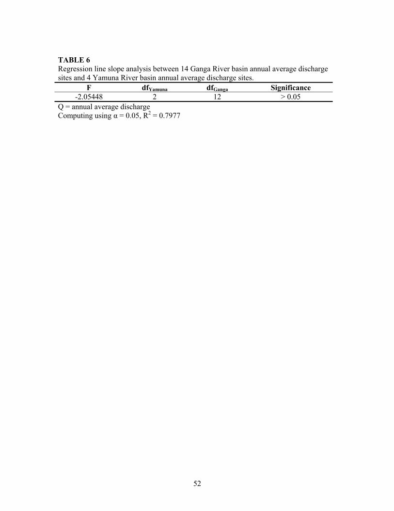
52

TABLE 6 Regression line slope analysis between 14 Ganga River basin annual average discharge sites and 4 Yamuna River basin annual average discharge sites.

F dfYamuna dfGanga Significance -2.05448 2 12 > 0.05

Q = annual average discharge Computing using α = 0.05, R2 = 0.7977

53

TABLE 7 Modeled discharge values based on reported discharge values (Rao 1975). Differ-ence in river discharge values (Reported Q – Modeled Q) also given.

River Station Observed Q (cms)

Predicted Q (cms)

% Difference

Ganga Hardwar 677 963 +29.7% Allahabad before Sangam 1670 1290 -29.5% Allahabad after Sangam 4304 6302 +31.7% Patna 10307 11639 +11.4% Farakka 12998 16953 +23.3% Yamuna Delhi 388 568 +31.7% Allahabad before Sangam 2634 2963 +11.1% Ramganga Confluence w/Ganga 432 416 -3.8% Gomati Confluence w/Ganga 209 378 +44.7% Ghaghara Confluence w/Ganga 2673 2188 -22.2% Gandak Confluence w/Ganga 1478 1135 -30.2% Tons Confluence w/Ganga 167 210 +20.5% Sone Confluence w/Ganga 900 732 -23.0% Kosi Confluence w/Ganga 1743 2194 +20.6% Bhuri Gandak Confluence w/Ganga 201 513 +60.8% Chambal Confluence w/Yamuna 851 854 +0.4% Betwa Confluence w/Yamuna 283 329 +14.0% Ken Confluence w/Yamuna 320 297 -7.7%

Average

difference +11.06

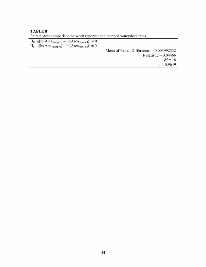
54

TABLE 8 Paired t-test comparison between reported and mapped watershed areas. H0: μ[ln(Areamapped) – ln(Areareported)] = 0 Ha: μ[ln(Areamapped) – ln(Areareported)] ≠ 0

Mean of Paired Differences = 0.003992532t-Statistic = 0.04466

df = 18p = 0.9649

55

TABLE 9 Multiple regression analysis of average annual discharge prediction model based on tributary watershed areas (km2), regional annual precipitation (mm/year), and the per-centage of the watershed originating in the Himalaya mountains.

R squared = 95.5% R squared (adjusted) = 94.4%s = 0.369 with 16 - 4 = 12 degrees of freedom

Source Sum of Squares df Mean Square F-ratio Regression 34.8317 3 11.6106 85.3 Residual 1.63416 12 0.13618 Variable Coefficient s.e. of Coeff t-ratio prob Constant -4.69783 0.7848 -5.99 ≤ 0.0001 ln(Area) 0.876326 0.06088 14.4 ≤ 0.0001 Precipitation 0.001192 4.53x10-04 2.63 0.0218 %Himalaya 1.00083 0.3267 3.06 0.0098

56

TABLE 10 Multiple regression analysis of the natural log of average annual BOD5 load prediction model based on total watershed population.

R squared = 74.5% R squared (adjusted) = 73.4%s = 0.7787 with 52 - 3 = 49 degrees of freedom

Source Sum of Squares df Mean Square F-ratio Regression 86.6972 2 43.3486 71.5 Residual 29.7133 49 0.606394 Variable Coefficient s.e. of Coeff t-ratio prob Constant -0.541658 1.038 -0.522 0.6040 ln(Q) 0.319948 0.1585 2.02 0.0491 ln(Poptotal) 0.435226 0.1193 3.65 0.0006 Q = river discharge (cms) Poptotal = Total upstream population

57

TABLE 11 Multiple regression analysis of the natural log of average annual total nitrogen load prediction model based on total watershed population.

R squared = 69.4% R squared (adjusted) = 67.9%s = 1.062 with 44 - 3 = 41 degrees of freedom

Source Sum of Squares df Mean Square F-ratio Regression 104.969 2 52.4843 46.6 Residual 46.2236 41 1.12741 Variable Coefficient s.e. of Coeff t-ratio prob Constant -3.55265 1.442 -2.46 0.0180 ln(Q) 0.0671292 0.2327 0.288 0.7744 ln(Poptotal) 0.723896 0.1681 4.31 0.0001 Q = river discharge (cms) Poptotal = Total upstream population

58

TABLE 12 Multiple regression analysis of the natural log of average annual total dissolved solid load prediction model based on watershed population, and annual average discharge.

R squared = 70.6% R squared (adjusted) = 69.4%s = 1.1 with 52 - 3 = 49 degrees of freedom

Source Sum of Squares df Mean Square F-ratio Regression 142.2 2 71.1002 58.8 Residual 59.2365 49 1.20891 Variable Coefficient s.e. of Coeff t-ratio prob Constant 1.23104 1.465 0.84 0.4049 ln(Q) 0.212352 0.2238 0.949 0.3474 ln(Poptotal) 0.698074 0.1685 4.14 0.0001 Q = river discharge (cms) Poptotal = Total upstream population

59

TABLE 13 Multiple regression analysis of the natural log of average annual total coliform concen-tration prediction model based on watershed population, and annual average discharge.

R squared = 33.4% R squared (adjusted) = 30.7%s = 2.42 with 52 - 3 = 49 degrees of freedom

Source Sum of Squares df Mean Square F-ratio Regression 144.02 2 72.0101 12.3 Residual 287.045 49 5.85806 Variable Coefficient s.e. of Coeff t-ratio prob Constant -5.7248 3.225 -1.78 0.0821 ln(Q) -1.51544 0.4927 -3.08 0.0034 ln(Poptotal) 1.67745 0.3709 4.52 ≤ 0.0001 Q = river discharge (cms) Poptotal = Total upstream population

60

TABLE 14 Regression of MLR-based nitrogen load calculation results against per capita maxi-mum potential daily maximum nitrogen load. The slope coefficient of “Nload” is the value of the estimated delivery ratio.

R squared = 25.0% R squared (adjusted) = 24.2%s = 8885 with 91 - 2 = 89 degrees of freedom

Source Sum of Squares df Mean Square F-ratio Regression 2.34675 x 109 1 2.34675 x 109 29.7 Residual 7.02654 x 109 89 78.9499 x 106 Variable Coefficient s.e. of Coeff t-ratio prob Constant -338.433 1256 -0.269 0.7882 Nload 2.85403 0.5235 5.45 ≤ 0.0001 Calculated nitrogen load based on MLR model.

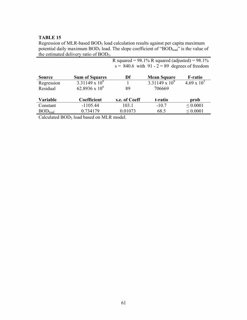
61

TABLE 15 Regression of MLR-based BOD5 load calculation results against per capita maximum potential daily maximum BOD5 load. The slope coefficient of “BODload” is the value of the estimated delivery ratio of BOD5.

R squared = 98.1% R squared (adjusted) = 98.1%s = 840.6 with 91 - 2 = 89 degrees of freedom

Source Sum of Squares Df Mean Square F-ratio Regression 3.31149 x 109 1 3.31149 x 109 4.69 x 103

Residual 62.8936 x 106 89 706669 Variable Coefficient s.e. of Coeff t-ratio prob Constant -1105.44 103.1 -10.7 ≤ 0.0001 BODload 0.734179 0.01073 68.5 ≤ 0.0001 Calculated BOD5 load based on MLR model.

62

TABLE 16 Modified classification of water quality, based on available modeled pollution parame-ters.

Class of Water Criteria A 1. Total Coliforms ≤ 50 MPN/100 ml

2. BOD5 ≤ 2 mg/l

B 1. Total Coliforms ≤ 500 MPN/100 ml 2. BOD5 ≤ 3 mg/l

C 1. Total Coliforms ≤ 5000 MPN/100 ml 2. BOD5 ≤ 4 mg/l

D 1. N ≤ 1.2 mg/l

E 1. Electrical Conductivity ≤ 2250 μmhos/cm

63

TABLE 17 Pre-GAP and post-GAP reported pollution concentrations from Central Pollution Con-trol Board, with comparison with the Danube River.

Danube (2002) Pre-GAP Post-GAP

Range of

Yearly Means Total Range Mean Min Max Mean Min Max

DO 6.7 - 11.6 3.2-26.3 7.4 0.1 92 7.3 0.3 22.8BOD 1.2 - 10.2 0.4-48.0 5.0 0.1 175 6.6 0.3 230COD 5.0 - 42.8 1.9-160 27.0 0.6 770.4 36.5 1 999.9NOx 0.55 - 4.69 0.05-8.23 5.9 0.001 80 0.1 0.001 3.54pH 7.2 - 8.3 6.4-9.0 8.0 1.5 13.8 7.9 2 10Fcoli N/A N/A 2.2 x105 1 2.4x108 2.3x107 1 1.87x1010Tcoli N/A N/A 2.5 x105 2 2.4x108 9.2x106 1 9.55x109Cond 217 - 954 140-1092 449.7 4 20000 514.9 10 11660Cl N/A N/A 38.7 1 3234 83.0 2 4674SO4 N/A N/A 29.2 1 2100 157.3 1 9999Na N/A N/A 32.9 1 16200 83.4 3 1328Ca N/A N/A 78.3 1 340 122.0 18 1140Mg N/A N/A 49.2 1 995 75.5 4 1330

TABLE 18 Water quality factors measured by the CPCB pre-GAP and post-GAP.

μ(Pre-Post)≠0 P-value

μ(Pre-Post)>0 P-value

μ(Pre-Post)<0 P-value

Pre-GAP Mean (ln)

Pre-GAP σ2 (ln)

Post-GAP Mean (ln)

Post-GAP σ2 (ln) t-stat df

mean paired difference (ln)

lnDO 0.1380 0.9310 0.0690 1.93 0.36 1.95 0.34 -1.515 38 0.256 lnBOD 0.0647 0.0323 0.9677 1.25 0.90 1.04 0.87 1.904 37 0.251 lnCOD 0.5885 0.2943 0.7057 3.04 0.79 2.92 0.79 0.546 38 0.078 lnNOx 0.0008 0.0004 0.9996 -0.41 1.58 -3.55 1.77 5.209 8 3.054 pH 0.8131 0.5934 0.4066 2.00 0.54 2.07 0.03 -0.238 33 -0.010 Temp 0.4520 0.7740 0.2260 3.14 0.67 3.16 0.23 -1.259 37 -0.212 Fcoli 0.1586 0.9207 0.0793 9.09 3.01 8.67 4.04 -1.439 37 -0.851 Tcoli 0.1947 0.9026 0.0974 9.94 2.91 10.62 3.48 -1.321 37 -0.684 lnAlkalinity 0.3041 0.8480 0.1520 4.69 1.08 4.94 0.61 -1.048 26 -0.253 lnChloride 0.3355 0.8323 0.1677 3.08 1.23 3.11 1.13 -0.977 34 -0.134 lnSO4 0.6578 0.3289 0.6711 3.16 0.94 3.29 1.16 0.447 32 0.072 lnNa 0.3359 0.8320 0.1680 2.66 1.01 2.97 0.82 -0.990 17 -0.113 lnCa 0.1277 0.9361 0.0639 4.13 0.94 4.49 0.56 -1.578 24 -0.367 lnMg 0.0608 0.9696 0.0304 3.61 0.95 3.98 0.60 -1.968 24 -0.418 lnTDS 0.0391 0.9805 0.0195 5.35 1.25 5.58 0.65 -2.139 37 -0.460 H0: μ[ln(GAPbefore)-ln(GAPafter)] = 0, Ha as indicated in the table. Italics indicate α<0.1. Bold indicates α<0.05

TABLE 19 Field sample results. Note that many of the samples needed to be diluted in order to be read by the instruments. Only half of the samples could gain a COD reading. The re-mainders indicate a known lower bound. City Date NH4 PO4 NO3-N CODHardwar 1/19/2004 < 0.01 < 0.01 0.02 > 5Kanpur (Water intake) 1/23/2004 2.75 1.26 0.14 > 25Kanpur (Kolya Ghat) 1/23/2004 0.1 6.2 0.74 >50Allahabad (Above Sangam) 1/26/2004 0.02 0.03 0.28 20Allahabad (Below Sangam) 1/26/2004 0.2 0.29 0.39 > 50Varanasi 2/8/2004 0.22 0.04 0.2 10Patna 1/29/2004 < 0.01 0.13 0.09 13Kolkata 2/4/2004 0.54 2.96 0.12 > 20

66

TABLE 20 Empirical loading estimates of calcium, chloride, BOD5, NOx, and TDS in Ganga River VSEC basins.

Q Watershed Pollutant Loading (kg/day) Pollutant Concentration (mg/L) Concentration (MPN/100 mL)Station ID cms Population Calcium Chloride BOD5 NOx TDS Calcium Chloride BOD5 NOx TDS Total Coliforms

3900 181.84 58972 273.72 61.14 31.66 9.97 1911.00 17.42 3.89 2.02 0.63 121.64 123.553820 138.22 15988 144.11 21.35 16.43 3.81 724.87 12.07 1.79 1.38 0.32 60.70 20.973810 286.11 35848 253.77 40.93 29.48 4.68 1486.45 10.27 1.66 1.19 0.19 60.13 26.973801 55.32 7948 62.49 12.16 9.04 2.16 366.37 13.07 2.54 1.89 0.45 76.65 26.003800 546.13 519372 1120.10 353.07 116.04 44.20 11021.60 23.74 7.48 2.46 0.94 233.58 897.373700 594.61 8039404 4006.36 3212.14 392.84 361.01 75965.78 77.98 62.52 7.65 7.03 1478.68 78116.133360 113.61 50120 141.76 53.63 25.38 8.59 1543.74 14.44 5.46 2.59 0.87 157.27 191.833350 129.96 59312 164.78 61.42 28.51 2.54 1786.60 14.67 5.47 2.54 0.23 159.11 207.543340 131.26 102416 213.66 95.40 36.28 7.78 2621.46 18.84 8.41 3.20 0.69 231.15 511.093330 238.35 2611828 1233.82 1297.90 179.76 153.40 28540.23 59.91 63.02 8.73 7.45 1385.87 47349.783320 326.30 6937900 2455.50 2852.43 304.07 232.38 60339.44 87.10 101.18 10.79 8.24 2140.31 151475.613310 416.15 12335106 3896.59 4535.72 422.23 277.23 94949.54 108.37 126.15 11.74 7.71 2640.77 275089.413230 45.12 2875606 796.32 1402.56 110.05 151.40 21435.03 204.28 359.79 28.23 38.84 5498.66 693222.593220 91.77 6121966 1653.63 2578.81 191.89 173.36 42235.56 208.57 325.26 24.20 21.87 5327.05 839655.063210 94.07 6355062 1702.81 2657.66 196.60 25.80 43581.06 209.50 326.98 24.19 3.17 5361.91 860949.033200 891.51 32241574 10263.00 9839.39 818.50 296.25 218294.58 133.24 127.74 10.63 3.85 2834.02 434514.853100 1289.70 34756938 10823.23 10453.56 951.76 172.10 248811.71 97.13 93.81 8.54 1.54 2232.90 281652.963000 67.53 40466 124.51 45.13 19.58 7.10 1190.52 21.34 7.74 3.36 1.22 204.04 294.712900 265.86 882464 889.06 541.27 116.08 70.10 13695.11 38.70 23.56 5.05 3.05 596.20 6500.302800 283.61 950532 952.00 574.68 122.40 11.40 14623.50 38.85 23.45 5.00 0.47 596.78 6676.332700 293.17 9806106 2586.02 3769.91 341.59 387.52 75098.04 102.09 148.83 13.49 15.30 2964.76 318314.452620 300.25 440972 931.24 309.44 89.24 44.25 8658.93 35.90 11.93 3.44 1.71 333.78 1688.422610 318.83 3204200 2089.34 1530.36 215.65 167.72 35015.27 75.85 55.55 7.83 6.09 1271.11 42931.352600 362.01 17442768 4482.85 5996.90 469.54 238.16 117403.35 143.32 191.73 15.01 7.61 3753.58 607590.762500 508.44 27046112 7371.50 8540.06 633.54 426.42 171388.43 167.81 194.41 14.42 9.71 3901.50 757872.682400 530.86 29719962 7910.33 9214.28 669.26 169.48 184732.80 172.46 200.89 14.59 3.70 4027.60 831508.312361 58.81 551120 539.84 370.36 58.36 46.61 7156.55 106.25 72.89 11.49 9.17 1408.52 29036.352360 131.70 2765934 1602.57 1359.28 152.44 134.67 26189.53 140.84 119.46 13.40 11.84 2301.60 128090.382350 172.65 4153454 2205.14 1886.35 198.41 97.76 36843.12 147.82 126.45 13.30 6.55 2469.82 168070.922340 197.77 4581490 2495.98 2041.53 216.26 42.11 40608.44 146.07 119.48 12.66 2.46 2376.56 161276.902330 396.80 9479410 4931.70 3668.35 370.82 257.59 78211.23 143.85 107.00 10.82 7.51 2281.31 190096.312320 408.22 10073226 5292.33 3852.46 384.22 56.03 82092.83 150.05 109.23 10.89 1.59 2327.56 201636.512310 853.61 24402686 11944.19 7860.67 715.04 589.87 178067.63 161.95 106.58 9.70 8.00 2414.40 290842.222230 61.84 813630 593.80 506.98 70.27 62.00 9493.74 111.14 94.89 13.15 11.60 1776.96 51721.642220 110.15 1843378 1238.57 980.10 120.66 76.43 18994.54 130.14 102.99 12.68 8.03 1995.88 85017.342210 213.59 6042650 2888.00 2551.84 250.03 221.05 50077.02 156.49 138.28 13.55 11.98 2713.55 228335.232200 1804.23 61143876 22330.74 16481.06 1355.01 88.87 396349.57 143.25 105.73 8.69 0.57 2542.57 436770.112150 156.04 2432214 1285.35 1225.47 152.18 145.76 24819.19 95.34 90.90 11.29 10.81 1840.93 79841.962140 220.71 3769774 1945.79 1744.60 205.76 96.78 36275.81 102.04 91.49 10.79 5.08 1902.32 98462.972130 255.16 5493840 2597.13 2363.33 253.92 117.44 48659.97 117.81 107.20 11.52 5.33 2207.21 148652.492120 210.27 6201706 2883.58 2605.85 251.61 60.86 50824.26 158.72 143.43 13.85 3.35 2797.52 244234.862114 15.88 131148 103.52 116.44 20.55 15.10 1989.35 75.46 84.88 14.98 11.01 1450.18 19003.752113 36.13 550656 292.22 370.11 49.92 37.02 6449.57 93.61 118.55 15.99 11.86 2065.93 60657.452112 118.76 2064662 1079.84 1073.87 129.85 101.54 20890.08 105.24 104.66 12.66 9.90 2035.89 91739.192111 97.37 2366802 1242.81 1198.83 129.32 31.20 22030.64 147.73 142.51 15.37 3.71 2618.81 155873.832110 328.92 9705132 4395.18 3738.59 352.81 88.35 76401.54 154.66 131.55 12.41 3.11 2688.39 262777.532100 2101.68 71827586 26116.34 18765.29 1526.11 89.79 458114.27 143.82 103.34 8.40 0.49 2522.87 454085.252050 206.79 2471328 1558.68 1241.33 167.69 150.27 26643.77 87.24 69.48 9.39 8.41 1491.22 53519.302040 245.57 2739900 1810.21 1348.96 185.30 30.49 29697.53 85.32 63.58 8.73 1.44 1399.70 49042.142030 281.46 3289390 2110.07 1563.07 209.59 51.66 34730.90 86.77 64.28 8.62 2.12 1428.17 54191.892020 300.98 3758964 2309.35 1740.56 226.94 46.32 38668.29 88.80 66.93 8.73 1.78 1486.96 61237.682010 297.24 4695888 2658.37 2082.52 249.03 76.30 45047.51 103.51 81.09 9.70 2.97 1754.06 90650.352000 2962.77 80915690 29376.52 20656.61 1793.98 272.45 535502.57 114.76 80.70 7.01 1.06 2091.95 329557.601900 3976.72 116064052 38689.54 27626.83 2306.22 48.28 733279.89 112.60 80.41 6.71 0.14 2134.18 386379.321820 196.75 2313420 1474.25 1176.99 160.36 142.78 25176.06 86.72 69.24 9.43 8.40 1480.98 51661.101810 210.07 2762638 1636.23 1357.97 176.91 43.78 28895.22 90.15 74.82 9.75 2.41 1592.04 63002.011800 4143.22 123241684 40733.08 28995.81 2398.52 279.70 771337.03 113.79 81.00 6.70 0.78 2154.73 401544.021722 18.10 605010 193.39 399.29 41.69 46.07 5946.94 123.70 255.39 26.66 29.47 3803.71 202578.571721 93.45 5750880 1469.66 2452.06 187.83 242.27 40587.76 182.03 303.71 23.26 30.01 5027.13 735528.881720 203.98 10174366 2651.16 3883.61 309.08 228.82 71343.22 150.43 220.36 17.54 12.98 4048.06 586741.211715 4.93 233736 72.05 185.51 18.18 21.21 2322.98 169.15 435.52 42.68 49.79 5453.49 294806.421714 71.88 2978142 1035.20 1442.73 129.70 151.01 24249.22 166.68 232.30 20.88 24.32 3904.48 362971.621713 132.59 4230246 1393.74 1914.41 183.80 89.16 35282.81 121.66 167.11 16.04 7.78 3079.83 258577.991712 165.15 5514826 1766.08 2370.61 221.30 92.17 44484.38 123.77 166.14 15.51 6.46 3117.53 289244.601711 178.14 5927268 1903.70 2512.50 233.95 40.71 47539.64 123.69 163.24 15.20 2.64 3088.71 291055.261710 377.51 16538532 4456.49 5745.04 464.98 44.63 114132.01 136.63 176.14 14.26 1.37 3499.21 521490.281700 4565.66 149770404 46816.21 33929.54 2693.29 508.44 902199.94 118.68 86.01 6.83 1.29 2287.10 480686.181640 422.48 208950 553.45 169.49 71.91 26.37 5527.47 15.16 4.64 1.97 0.72 151.43 287.471630 1332.09 622730 1769.05 408.69 167.03 46.70 15118.15 15.37 3.55 1.45 0.41 131.36 315.031620 1389.98 696920 1852.59 447.50 177.82 13.50 16502.35 15.43 3.73 1.48 0.11 137.41 356.751614 28.58 183622 142.97 152.72 28.72 20.04 2850.64 57.91 61.86 11.63 8.12 1154.58 13716.161613 185.51 3121136 1396.23 1498.31 179.28 169.06 30644.50 87.11 93.48 11.19 10.55 1911.89 93336.001612 246.98 5053576 2033.33 2209.46 242.32 127.27 45587.00 95.29 103.54 11.36 5.96 2136.34 135761.101611 270.24 5831798 2292.23 2479.83 265.44 66.28 51352.90 98.17 106.21 11.37 2.84 2199.40 150618.451610 2187.76 22223930 11083.24 7289.91 927.74 671.14 203717.30 58.63 38.57 4.91 3.55 1077.74 59718.111540 29.94 193654 180.39 159.41 29.83 20.89 2988.00 69.73 61.62 11.53 8.08 1154.93 13970.481530 45.61 380708 300.73 274.88 45.80 20.96 5237.36 76.32 69.76 11.62 5.32 1329.13 22948.541520 71.96 887870 544.12 543.94 76.62 44.49 10420.47 87.52 87.49 12.32 7.16 1676.13 47592.581512 31.04 137864 164.50 121.22 26.03 16.38 2375.12 61.33 45.20 9.70 6.11 885.55 7480.851511 172.51 1551050 1178.12 852.76 129.20 99.06 18520.52 79.04 57.21 8.67 6.65 1242.60 32245.431510 732.40 10297188 5889.81 3921.35 467.70 377.94 94379.90 93.08 61.97 7.39 5.97 1491.48 86273.941450 668.22 1119322 1333.00 655.61 172.89 91.64 19662.71 23.09 11.36 2.99 1.59 340.57 2396.481440 1132.03 2519634 2498.34 1260.85 291.33 111.65 38747.85 25.54 12.89 2.98 1.14 396.17 4204.721430 1137.98 2577128 2526.65 1283.99 294.69 11.07 39406.78 25.70 13.06 3.00 0.11 400.80 4332.361420 1133.86 5074490 3466.11 2216.82 395.31 169.74 63190.19 35.38 22.63 4.04 1.73 645.02 13574.031410 1134.69 5596828 3626.54 2398.98 412.63 54.69 67673.71 36.99 24.47 4.21 0.56 690.28 15980.911400 7406.21 190911170 64164.25 41260.52 3494.44 221.07 1184396.53 100.27 64.48 5.46 0.35 1850.92 346969.211310 513.40 14501974 4292.14 5167.67 484.53 575.04 111154.02 96.76 116.50 10.92 12.96 2505.83 262511.411220 2880.65 1281360 2601.39 731.08 292.65 111.47 29470.26 10.45 2.94 1.18 0.45 118.41 328.411210 2194.30 7019050 5285.18 2879.29 562.33 324.00 91177.43 27.88 15.19 2.97 1.71 480.93 8600.181200 9532.41 228625306 75948.38 47713.23 4097.52 757.78 1417185.22 92.22 57.93 4.98 0.92 1720.72 320273.53

67

TABLE 21 Per capita loading estimates of BOD, nitrogen, and TDS in Ganga River VSEC units.

Population Q Population Pollutant Loading (kg/day) Pollutant Concentration (mg/L) Station ID 50 km U/S cms Watershed Nitrogen BOD5 Phosphate Nitrogen BOD5 Phosphate

3900 17990 181.84 58972 43.83 6.77 18.74 0.24 0.04 0.10 3820 4754 138.22 15988 11.88 1.83 0.50 0.09 0.01 0.00 3810 7723 286.11 35848 26.64 4.11 0.80 0.09 0.01 0.00 3801 3892 55.32 7948 5.91 0.91 0.41 0.11 0.02 0.01 3800 166931 546.13 519372 386.02 59.58 17.39 0.71 0.11 0.03 3700 500833 594.61 8039404 5975.18 922.24 52.17 10.05 1.55 0.09 3360 1621 113.61 50120 37.25 5.75 0.17 0.33 0.05 0.00 3350 8155 129.96 59312 44.08 6.80 0.85 0.34 0.05 0.01 3340 38529 131.26 102416 76.12 11.75 4.01 0.58 0.09 0.03 3330 557278 238.35 2611828 1941.21 299.62 58.05 8.14 1.26 0.24 3320 376811 326.30 6937900 5156.50 795.88 39.25 15.80 2.44 0.12 3310 6996 416.15 12335106 9167.91 1415.03 0.73 22.03 3.40 0.00 3230 249298 45.12 2875606 2137.26 329.88 25.97 47.37 7.31 0.58 3220 138467 91.77 6121966 4550.07 702.28 14.42 49.58 7.65 0.16 3210 256325 94.07 6355062 4723.32 729.02 26.70 50.21 7.75 0.28 3200 237069 891.51 32241574 23963.13 3698.61 24.69 26.88 4.15 0.03 3100 208396 1289.70 34756938 25832.64 3987.16 21.71 20.03 3.09 0.02 3000 14720 67.53 40466 30.08 4.64 1.53 0.45 0.07 0.02 2900 29887 265.86 882464 655.88 101.23 3.11 2.47 0.38 0.01 2800 139724 283.61 950532 706.47 109.04 14.55 2.49 0.38 0.05 2700 3717277 293.17 9806106 7288.26 1124.91 387.22 24.86 3.84 1.32 2620 61355 300.25 440972 327.75 50.59 6.39 1.09 0.17 0.02 2610 529412 318.83 3204200 2381.48 367.57 55.15 7.47 1.15 0.17 2600 1000882 362.01 17442768 12964.11 2000.96 104.26 35.81 5.53 0.29 2500 1228627 508.44 27046112 20101.67 3102.61 127.98 39.54 6.10 0.25 2400 405726 530.86 29719962 22088.98 3409.34 42.26 41.61 6.42 0.08 2361 57000 58.81 551120 409.61 63.22 5.94 6.97 1.08 0.10 2360 117529 131.70 2765934 2055.74 317.30 12.24 15.61 2.41 0.09 2350 174517 172.65 4153454 3087.00 476.47 18.18 17.88 2.76 0.11 2340 133970 197.77 4581490 3405.13 525.57 13.96 17.22 2.66 0.07 2330 858789 396.80 9479410 7045.45 1087.44 89.46 17.76 2.74 0.23 2320 126079 408.22 10073226 7486.79 1155.55 13.13 18.34 2.83 0.03 2310 69387 853.61 24402686 18136.98 2799.37 7.23 21.25 3.28 0.01 2230 109478 61.84 813630 604.72 93.34 11.40 9.78 1.51 0.18 2220 45710 110.15 1843378 1370.07 211.46 4.76 12.44 1.92 0.04 2210 319770 213.59 6042650 4491.12 693.19 33.31 21.03 3.25 0.16 2200 425572 1804.23 61143876 45444.39 7014.15 44.33 25.19 3.89 0.02 2150 269891 156.04 2432214 1807.71 279.01 28.11 11.58 1.79 0.18 2140 187261 220.71 3769774 2801.84 432.45 19.51 12.69 1.96 0.09 2130 331617 255.16 5493840 4083.23 630.23 34.54 16.00 2.47 0.14 2120 161840 210.27 6201706 4609.34 711.43 16.86 21.92 3.38 0.08 2114 62241 15.88 131148 97.47 15.04 6.48 6.14 0.95 0.41 2113 100051 36.13 550656 409.27 63.17 10.42 11.33 1.75 0.29 2112 74981 118.76 2064662 1534.53 236.85 7.81 12.92 1.99 0.07 2111 114064 97.37 2366802 1759.09 271.51 11.88 18.07 2.79 0.12 2110 119571 328.92 9705132 7213.21 1113.33 12.46 21.93 3.38 0.04 2100 425572 2101.68 71827586 53384.92 8239.74 44.33 25.40 3.92 0.02 2050 152686 206.79 2471328 1836.78 283.50 15.90 8.88 1.37 0.08 2040 150421 245.57 2739900 2036.40 314.31 15.67 8.29 1.28 0.06 2030 64485 281.46 3289390 2444.80 377.34 6.72 8.69 1.34 0.02 2020 102628 300.98 3758964 2793.80 431.21 10.69 9.28 1.43 0.04 2010 373202 297.24 4695888 3490.16 538.69 38.88 11.74 1.81 0.13 2000 152166 2962.77 80915690 60139.53 9282.28 15.85 20.30 3.13 0.01 1900 806956 3976.72 116064052 86263.10 13314.34 84.06 21.69 3.35 0.02 1820 376218 196.75 2313420 1719.42 265.39 39.19 8.74 1.35 0.20 1810 256731 210.07 2762638 2053.29 316.92 26.74 9.77 1.51 0.13 1800 786654 4143.22 123241684 91597.78 14137.73 81.94 22.11 3.41 0.02 1722 294241 18.10 605010 449.67 69.40 30.65 24.85 3.84 1.69 1721 1021893 93.45 5750880 4274.27 659.71 106.45 45.74 7.06 1.14 1720 191664 203.98 10174366 7561.97 1167.16 19.97 37.07 5.72 0.10 1715 108755 4.93 233736 173.72 26.81 11.33 35.24 5.44 2.30 1714 289882 71.88 2978142 2213.47 341.64 30.20 30.79 4.75 0.42 1713 293241 132.59 4230246 3144.08 485.27 30.55 23.71 3.66 0.23 1712 613068 165.15 5514826 4098.82 632.64 63.86 24.82 3.83 0.39 1711 87843 178.14 5927268 4405.36 679.95 9.15 24.73 3.82 0.05 1710 276199 377.51 16538532 12292.05 1897.23 28.77 32.56 5.03 0.08 1700 158190 4565.66 149770404 111314.90 17180.98 16.48 24.38 3.76 0.00 1640 37129 422.48 208950 155.30 23.97 3.87 0.37 0.06 0.01 1630 48787 1332.09 622730 462.84 71.44 5.08 0.35 0.05 0.00 1620 38784 1389.98 696920 517.98 79.95 4.04 0.37 0.06 0.00 1614 92331 28.58 183622 136.47 21.06 9.62 4.78 0.74 0.34 1613 466759 185.51 3121136 2319.74 358.04 48.62 12.50 1.93 0.26 1612 393856 246.98 5053576 3756.00 579.72 41.03 15.21 2.35 0.17 1611 359338 270.24 5831798 4334.41 669.00 37.43 16.04 2.48 0.14 1610 286339 2187.76 22223930 16517.65 2549.43 29.83 7.55 1.17 0.01 1540 18882 29.94 193654 143.93 22.22 1.97 4.81 0.74 0.07 1530 12924 45.61 380708 282.96 43.67 1.35 6.20 0.96 0.03 1520 263085 71.96 887870 659.90 101.85 27.40 9.17 1.42 0.38 1512 50522 31.04 137864 102.47 15.82 5.26 3.30 0.51 0.17 1511 132988 172.51 1551050 1152.80 177.93 13.85 6.68 1.03 0.08 1510 512476 732.40 10297188 7653.25 1181.25 53.38 10.45 1.61 0.07 1450 198266 668.22 1119322 831.92 128.40 20.65 1.24 0.19 0.03 1440 58868 1132.03 2519634 1872.69 289.04 6.13 1.65 0.26 0.01 1430 216943 1137.98 2577128 1915.42 295.64 22.60 1.68 0.26 0.02 1420 251512 1133.86 5074490 3771.55 582.12 26.20 3.33 0.51 0.02 1410 272520 1134.69 5596828 4159.77 642.04 28.39 3.67 0.57 0.03 1400 1000000 7406.21 190911170 141892.24 21900.46 104.17 19.16 2.96 0.01 1310 311574 513.40 14501974 10778.40 1663.60 32.46 20.99 3.24 0.06 1220 90568 2880.65 1281360 952.35 146.99 9.43 0.33 0.05 0.00 1210 625733 2194.30 7019050 5216.82 805.19 65.18 2.38 0.37 0.03 1200 374577 9532.41 228625306 169922.78 26226.86 39.02 17.83 2.75 0.00

68

TABLE 22 Ratio of MLR estimates of nitrogen and BOD5 against per capita estimates. Per capita estimates are comparatively lower than MLR estimates.

MLR estimate/per capita estimate Station ID Nitrogen BOD

3900 261.37 54.30 3820 372.21 104.00 3810 204.03 82.79 3801 421.41 114.67 3800 132.99 22.55 3700 69.96 4.93 3360 265.34 51.18 3350 67.81 48.52 3340 118.98 35.75 3330 91.48 6.94 3320 52.14 4.42 3310 35.00 3.45 3230 81.99 3.86 3220 44.11 3.16 3210 6.31 3.12 3200 14.32 2.56 3100 7.69 2.76 3000 273.94 48.88 2900 123.63 13.26 2800 18.87 13.00 2700 61.55 3.52 2620 156.66 20.42 2610 81.53 6.79 2600 21.25 2.72 2500 24.56 2.36 2400 8.89 2.27 2361 131.65 10.69 2360 75.85 5.56 2350 36.63 4.82 2340 14.29 4.76 2330 42.30 3.95 2320 8.67 3.85 2310 37.65 2.96 2230 118.62 8.71 2220 64.56 6.60 2210 56.98 4.18 2200 2.26 2.24 2150 93.31 6.31 2140 40.02 5.51 2130 33.31 4.66 2120 15.28 4.09 2114 179.34 15.81 2113 104.71 9.15 2112 76.62 6.35 2111 20.53 5.51 2110 14.18 3.67 2100 1.93 2.14 2050 94.68 6.85 2040 17.36 6.82 2030 24.41 6.43 2020 19.18 6.09 2010 25.29 5.35 2000 5.22 2.24 1900 0.65 2.00 1820 96.12 6.99 1810 24.66 6.46 1800 3.53 1.96 1722 118.59 6.95 1721 65.61 3.29 1720 35.01 3.07 1715 141.30 7.85 1714 78.98 4.39 1713 32.81 4.38 1712 26.03 4.05 1711 10.68 3.98 1710 4.21 2.84 1700 5.29 1.81 1640 195.87 34.72 1630 118.00 27.04 1620 29.52 25.73 1614 170.02 15.78 1613 84.37 5.80 1612 39.19 4.84 1611 17.71 4.59 1610 47.02 4.21 1540 168.10 15.54 1530 85.75 12.13 1520 78.07 8.70 1512 185.11 19.04 1511 99.51 8.41 1510 57.13 4.58 1450 127.71 15.56 1440 68.91 11.67 1430 6.54 11.55 1420 52.01 7.87 1410 15.28 7.44 1400 1.83 1.85 1310 61.73 3.37 1220 136.11 23.12 1210 71.93 8.09 1200 5.16 1.81

Mean 76.25 12.76 Std Deviation 79.58 19.90

69

TABLE 23 Number of VSEC river miles with falling into CPCB-based water quality classes. Hi-malaya Tributaries include Ramganga, Ghaghara, Gandak, Bhuri Gandak, Kosi, and Yamuna Rivers. Other Tributaries include Gomati, Chambal, Betwa, Kens, Tons, Sone, Sind, and Hooghly Rivers. The Hooghly River and the Ganga River downstream of Farakka were not modeled.

CPCB water quality

classes Entire

WatershedGanga

MainstemHimalayan Tributaries

Non-Himalayan Tributaries

A 129 129 0 0B 710 103 608 0C 425 81 344 0D 983 466 517 0E 1,236 0 827 409

Worse than E 5,249 654 1,237 3,358Totals 8,731 1,432 3,533 3,767

70

TABLE 24 CPCB’s 2002 “Revised Water Quality Criteria” Criteria Parameter A – Excellent B – Desirable C – Acceptable pH 7.0 to 8.5 6.5 to 9.0 6.5 to 9.0 DO (% saturation) 90 to 110 80 to 120 60 to 140 BOD (mg/L) < 2 < 3 < 6 Conductivity < 1000 < 2250 < 4000 NO2+NO3 (mg/L) < 5 < 10 < 15 Suspended Solids (mg/L) < 25 < 50 < 100 Fecal coliform (MPN/100 mL) < 20 < 200 < 2000 Bioassay (Zebra fish) No death in 5

days No death in 3

days No death in 2

days

71

TABLE 25 Comparison of the number of CPCB sites in each water quality category using the 2002 altered criteria against the original criteria in (year=2003). Percent attainment in years 2002 and 2003 are compared to the percent of river miles in each water quality class based on the results from the MLR models. Water Quality Class Year A B C D E Below E 2002 9 (8.7%) 43 (41.7%) 51 (49.5%) - - - - - - 2003 0 (0.0%) 11 (9.7%) 29 (25.7%) 19 (16.8%) 46 (40.7%) 8 (7.1%) Modeled - (1.5%) - (8.1%) - (4.9%) - (11.3%) - (14.2%) - (60.1%)

72

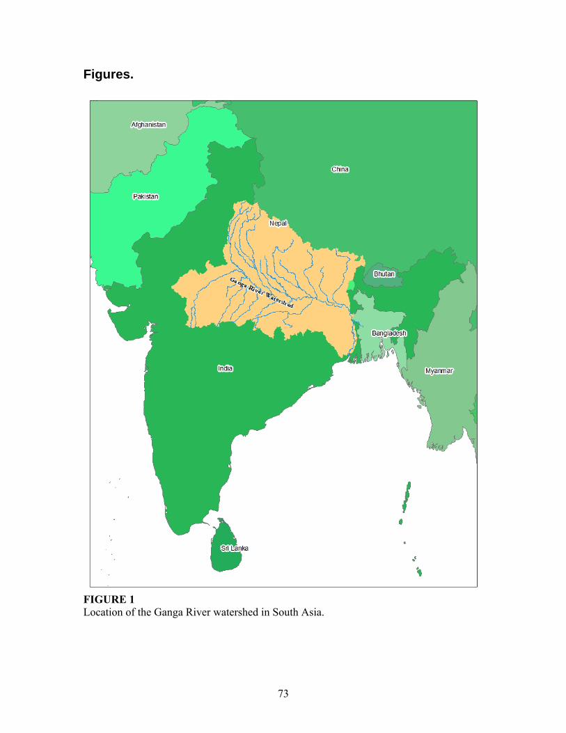
73

Figures.

FIGURE 1 Location of the Ganga River watershed in South Asia.

74

FIGURE 2 The Ganga River basin, with the Himalaya Mountains to the north and the Vindhya Mountains to the south.

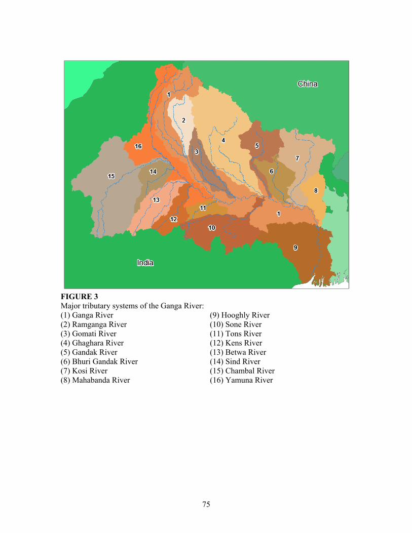
75

FIGURE 3 Major tributary systems of the Ganga River: (1) Ganga River (9) Hooghly River (2) Ramganga River (10) Sone River (3) Gomati River (11) Tons River (4) Ghaghara River (12) Kens River (5) Gandak River (13) Betwa River (6) Bhuri Gandak River (14) Sind River (7) Kosi River (15) Chambal River (8) Mahabanda River (16) Yamuna River

76

0

10000

20000

30000

40000

50000

60000

J F M A M J J A S O N D

Month

Disc

harg

e (c

ubic

feet

per

sec

ond)

FIGURE 4 Average monthly discharge (1949 – 1960, 1965 – 1973) of the Ganga River at the Farakka. Error bars indicate one standard deviation.

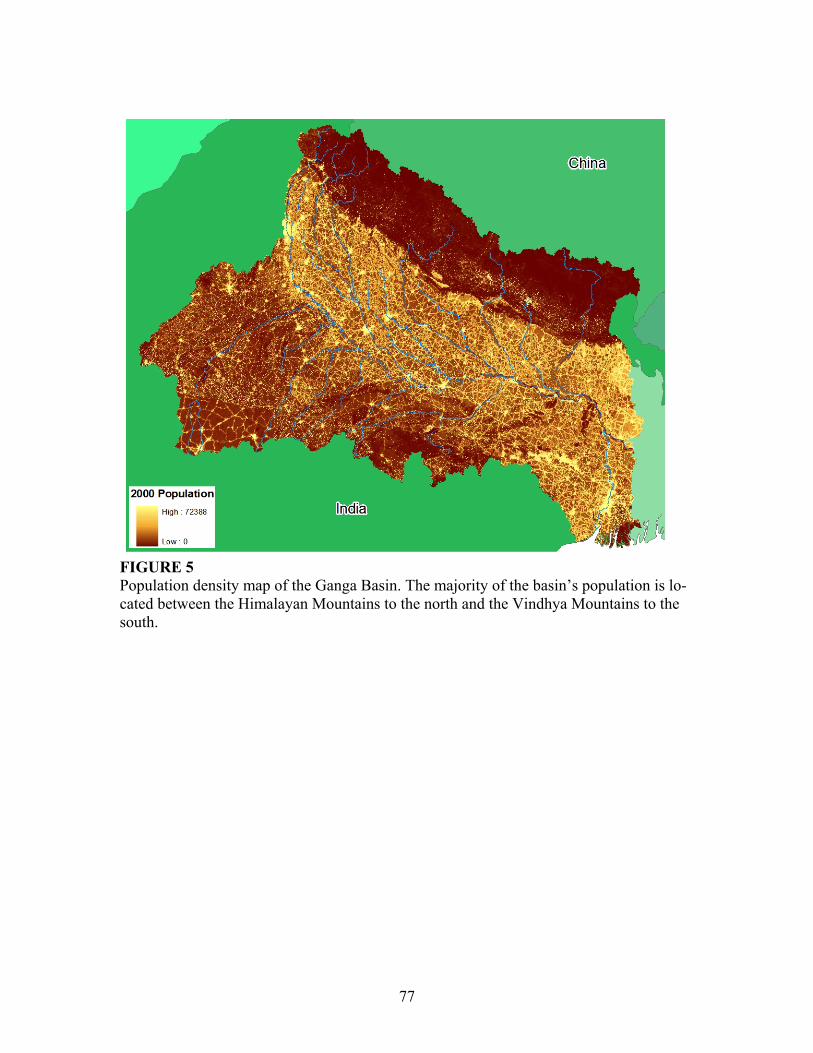
77

FIGURE 5 Population density map of the Ganga Basin. The majority of the basin’s population is lo-cated between the Himalayan Mountains to the north and the Vindhya Mountains to the south.

78

FIGURE 6 Regression analysis of the Ganga basin station geometries requires an extrapolation to larger and smaller basin areas than found in Rao (1975). This was accomplished by using world river data for a wide variety of rivers. Sites with larger and smaller basin areas are indicated in the circles.

World River station geometries

0.0000

1.0000

2.0000

3.0000

4.0000

5.0000

6.0000

2.0000 3.0000 4.0000 5.0000 6.0000 7.0000

log(Area)

log(

Q)

World Rivers

Linear (World Rivers)

Ganga River station geometries

0.0000

1.0000

2.0000

3.0000

4.0000

5.0000

6.0000

2.0000 3.0000 4.0000 5.0000 6.0000 7.0000

log(Area)

log(

Q)

Ganga

Linear (Ganga)

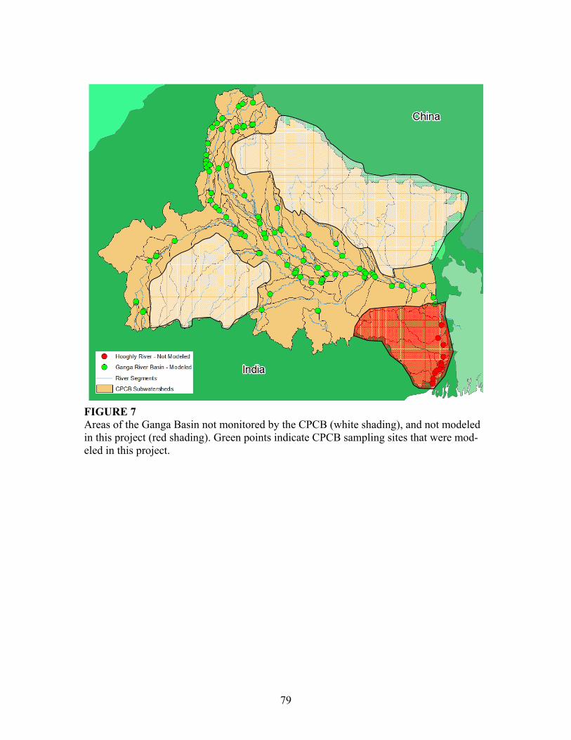
79

FIGURE 7 Areas of the Ganga Basin not monitored by the CPCB (white shading), and not modeled in this project (red shading). Green points indicate CPCB sampling sites that were mod-eled in this project.

80

FIGURE 8 Location of modeled ninety VSEC sites, and their corresponding upstream watershed ar-eas. The Hooghly River system (red shading) was not modeled.

81

FIGURE 9 Water sampling locations visited during personal trip to India in January and February 2004. Path indicates order of sampling.

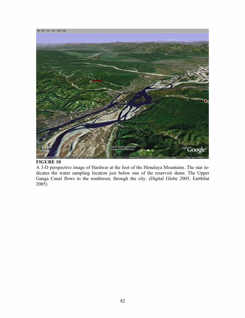
82

FIGURE 10 A 3-D perspective image of Hardwar at the foot of the Himalaya Mountains. The star in-dicates the water sampling location just below one of the reservoir dams. The Upper Ganga Canal flows to the southwest, through the city. (Digital Globe 2005, EarthSat 2005)

83

FIGURE 11 A 3-D rendered perspective image of Kanpur, with the two sampling sites shown with stars. The western site is the water intake site, and the other is the Kolya Ghat site. The river is flowing from the northwest to the southeast in this view.

84

FIGURE 12 Water intake canal in Kanpur. Both banks of the canal are lined with shanties. Upstream of the canal is an outfall from a tuberculosis hospital.

85

FIGURE 13 Ganga River at Kolya Ghat in Kanpur.

86

FIGURE 14 A 3-D rendered perspective of Allahabad. The two sampling sites are marked with stars. Note the confluence of the Yamuna River (from the west) with the Ganga River (from the north). the location the sandy spit at the confluence point was the main gathering point of the thousands of Ardh Kumbh Mela pilgrims.

87

FIGURE 15 Looking downstream along the banks of the Ganga, roughly 2km downstream of the San-gam, near Allahabad.

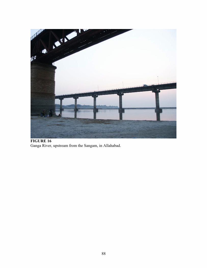
88

FIGURE 16 Ganga River, upstream from the Sangam, in Allahabad.

89

FIGURE 17 A 3-D rendered perspective image of Varanasi. The water sampling site is shown with the star. The Ganga River flows from the south to the east and north.

90

FIGURE 18 Sampling point in Varanasi, looking downstream.

91

FIGURE 19 A 3-D rendered perspective of the water sampling site in Patna. Note the confluence of two major tributaries from the northwest and the north. The Ganga continues toward the east, splitting around a major island.

92

FIGURE 20 Sampling location on the Ganga River, downstream of Patna.

93

FIGURE 21 A 3-D rendered perspective of the Kolkata metropolitan area. The water sampling site is shown with a star, and is just opposite of the Botanical Gardens. Although this stretch of the Hooghly River is still considered “sweetwater,” the flow of the river is heavily influ-enced by the tides. The river meanders in this aerial view from the north and exits to the west.

94

FIGURE 22 Calculated BOD5 concentrations based on derived MLR equation for each VSEC river unit throughout the Ganga basin. Categories coded by quantiles.

95

FIGURE 23 Calculated nitrogen concentrations based on derived MLR equation for each VSEC river unit throughout the Ganga basin. Categories coded by quantiles.

96

FIGURE 24 Calculated TDS concentrations based on derived MLR equation for each VSEC river unit throughout the Ganga basin. Categories coded by quantiles.

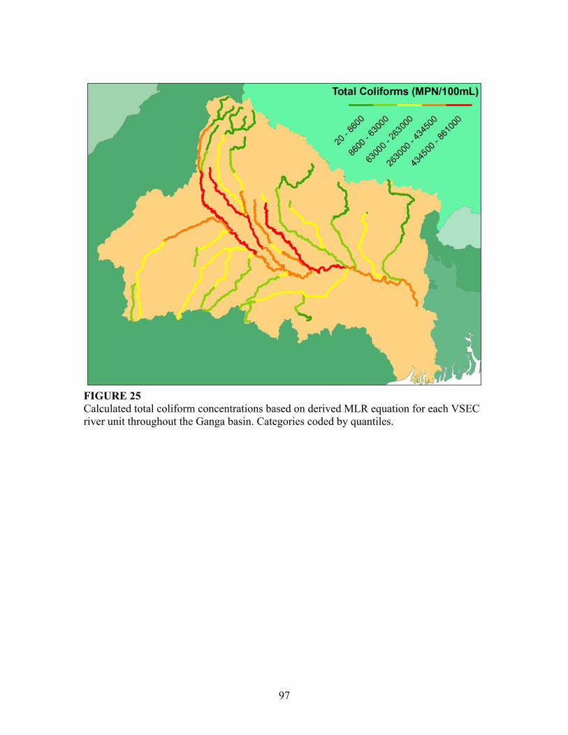
97

FIGURE 25 Calculated total coliform concentrations based on derived MLR equation for each VSEC river unit throughout the Ganga basin. Categories coded by quantiles.

98

FIGURE 26 Calculated BOD5 concentrations based on standard per capita equation for each VSEC river unit throughout the Ganga basin. Categories coded by quantiles.

99

FIGURE 27 Calculated total nitrogen concentrations based on standard per capita equation for each VSEC river unit throughout the Ganga basin. Categories coded by quantiles.

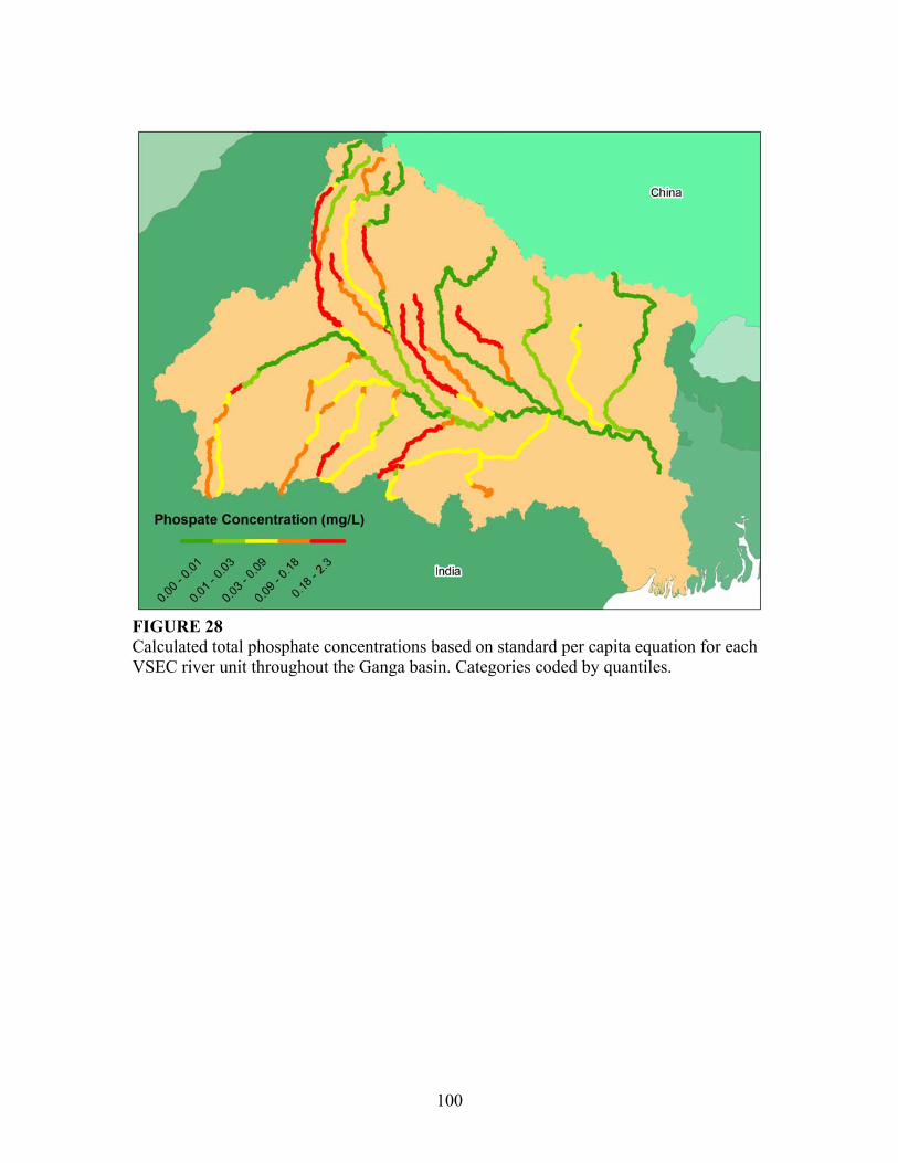
100

FIGURE 28 Calculated total phosphate concentrations based on standard per capita equation for each VSEC river unit throughout the Ganga basin. Categories coded by quantiles.

101

FIGURE 29 Classification of waters into classes A, B, C and “worse than C” based on CPCB’s water quality parameters of BOD concentration. Values of BOD estimated using empirical loading model.

102

FIGURE 30 Classification of waters into classes A, B, C and “worse than C” based on CPCB’s water quality parameters of total coliform counts. Values of total coliforms estimated using empirical loading model.

103

FIGURE 31 Classification of waters into classes D and “worse than D” based on CPCB’s water qual-ity parameters of nitrogen concentration. Values of nitrogen estimated using empirical loading model.

104

FIGURE 32 Classification of waters into classes E and “worse than E” based on CPCB’s water quality parameters of conductivity. Values of conductivity estimated using empirical loading model.

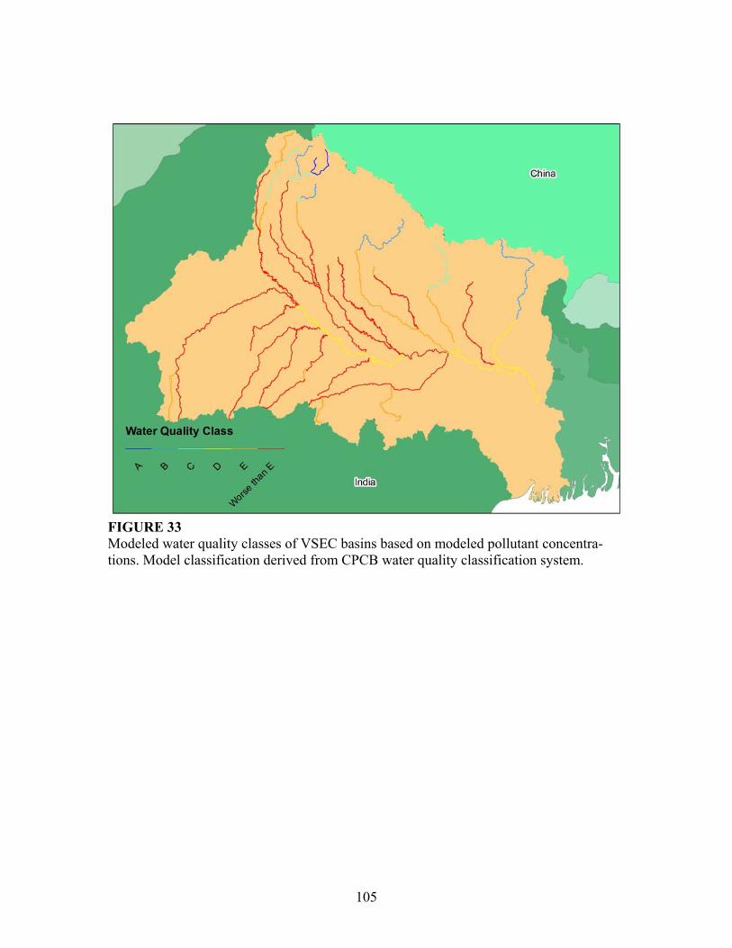
105

FIGURE 33 Modeled water quality classes of VSEC basins based on modeled pollutant concentra-tions. Model classification derived from CPCB water quality classification system.

106

FIGURE 34 The city of Kanpur lies just outside the 50km upstream radius from the VSEC subbasin output point.

107

FIGURE 35 Section of bathers present at the Ardh Kumbh Mela pilgrimage at the confluence of Ya-muna and Ganga Rivers at Allahabad.

108

FIGURE 36 Relative comparison of water present in the Ganga River (top) and the Yamuna River (bottom) before their confluence, Allahabad.

109

FIGURE 37 Setup of VSEC subbasins around the city of Allahabad. The city is split roughly in half between the Yamuna River and Ganga River subbasins upstream of the confluence point. The entire city of Allahabad is within 50km of the downstream VSEC Subbasin output point, and has been included within the phosphate model at the downstream end.

110

111

Bibliography

Adel, MM (2001) “Effect of Water Resources of Upstream Water Diversion in the Ganges Basin” J. Environ. Qual. (30) 356-368.

Ahmad, QK, AK Biwas, R Rangashari, MM Sainju (Eds) (2001) Ganges-Brahmaputra-Meghna Region: A Framework for Sustainable Development, The University Press, Dhaka.

Alley, KD (2002) On the Banks of the Ganga: When Wastewater Meets a Sacred River, University of Michigan Press, Ann Arbor.

Basu, AK (1992) Ecological and Resource Study of the Ganga Delta, KP Bagchi & Company, Calcutta.

Bilgrami, KS (1991) “Biological Profile of the Ganga: Bacteria and Bacteriophages” from The Ganga: A Scientific Study, Krishna Murti, C.R., K.S. Bilgrami, T.M. Das, and R.P. Mathur (eds), Northern Book Centre, New Delhi

Census of India (2000), Census of India 2000

Central Pollution Control Board (1985) Water Quality Yearbook 1980-1987

Central Pollution Control Board (1998) Water Quality Yearbook 1998

Central Pollution Control Board (CPCB) (2002) “Core Water Quality Monitoring Pa-rameters” (http://www.cpcb.nic.in/Watdata2002/criteria.htm)

Central Pollution Control Board (2003) Water Quality Yearbook 2003

Data Description, Inc (1996) Data Desk, version 6.1, Ithaca, NY.

Datta, N.C. (1991) “Assessment of Pollution Load on the Ganga in the Stretch Bally to Bandel” from The Ganga: A Scientific Study, Krishna Murti, C.R., K.S. Bilgrami, T.M. Das, and R.P. Mathur (eds), Northern Book Centre, New Delhi

ESRI (2005) ArcMap, version 9.1 (Build 722), Redlands, CA.

European Union (EU) (2005) “Bathing Water Quality” Directive 76/160/EEC (http://europa.eu.int/water/water-bathing/directiv.html)

Google, Inc (2005) GoogleEarth, version 3.0.0336

Gourdji, S., C. Knowlton, K. Platt (2005) Indian Inter-linking of Rivers: A Preliminary Evaluation, University of Michigan, School of Natural Resources and Environ-ment, Master’s Project

Hinrichsen, D & H Tacio (1997) “The Coming Freshwater Crisis is Already Here from Finding the Source: The Linkages Between Population and Water, Woodrow Wilson Center, Washington, D.C.

International Commission for the Protection of the Danube River (ICPDR) (2003) Water Quality in the Danube River Basin, TNMN Yearbook 2002, Permanent Secretariat, Vienna, Austria (http://www.icpdr.org/icpdr-pages/tnmn_yearbooks.htm)

112

Krishna Murti, C.R., K.S. Bilgrami, T.M. Das, and R.P. Mathur (eds) (1991) The Ganga: A Scientific Study, Northern Book Centre, New Delhi

Leopold, LB (1994) A View of the River, Harvard University Press.

Maiti, P. and S. Banerjee (2002) “Bioaccumulation of Metals in Different Food Fishes in Wastewater Fed Wetlands” from Ecology of Polluted Waters, Kumar, A (editor), A.P.H. Publishing Corporation, New Delhi.

Markandya A & MN Murty (2000) Cleaning up the Ganges: A Cost Benefit Analysis of the Ganga Action Plan, Oxford University Press, Delhi.

Mathur, R.P. (1991) “Trend of Physico-Chemical Characteristics of the Ganga Water”, from The Ganga: A Scientific Study, Krishna Murti, C.R., K.S. Bilgrami, T.M. Das, and R.P. Mathur (eds), Northern Book Centre, New Delhi

Ministry of Environment and Forests (MoEF) (1995) Evaluation of Ganga Action Plan, Government of India, New Delhi.

Ministry of Environment and Forests (MoEF), Public Accounts Committee (2004) Ganga Action Plan. Lok Sabha Secretariat, New Delhi.

National Imagery and Mapping Agency (1998) VMap Level 0, NIMA, Bethesda.

National River Conservation Directorate (1999a) Bulletin for Water Quality Monitoring and Performance of Sewage Treatment Plants, Ministry of the Environment and Forests, Government of India, New Delhi.

National River Conservation Directorate (1999b) Status on River Action Plan, Ministry of the Environment and Forests, Government of India, New Delhi.

Niemczynowicz, J., A Tyagi, V.K. Dwivedi (1998) “Water and environment in India: re-lated problems and possible solutions” Water Policy 1: 209-222

Pandey, U.K. (1991) “Physico-Chemical Studies of the Ganga Water at Kanpur (Kan-nauj to Shuklaganj Sector)”, from The Ganga: A Scientific Study, Krishna Murti, C.R., K.S. Bilgrami, T.M. Das, and R.P. Mathur (eds), Northern Book Centre, New Delhi

Raina, V, Chowdhury, A, Chowdhury S (1997) The Disposessed: Victims of Develop-ment in Asia, Arena Press, Hong Kong.

Rao, KL (1975) India’s Water Wealth: Its Assessment, Uses, and Projections, Orient Longman, New Delhi.

Rao, RJ (2001) “Biological Resources of the Ganga River, India” Hydrobiologia (458) 159-168.

Ray, P (1998) Ecological Imbalance of the Ganga River System: Its Impact on Aquacul-ture, Daya Publishing House, Delhi.

Sabata, BC & Nayar, MP (1995) River Pollution in India: A Case Study of Ganga River, APH Publishing, New Delhi.

113

Saha, T., P.B. Ghosh, C.C. Mondal and T.S. Bandyopadhyay (2002) “Ecology of some canals of Kolkata in relation to bacterial population” from Ecology of Polluted Waters, Kumar, A (editor), A.P.H. Publishing Corporation, New Delhi.

Schwoerbel, J (1987) Handbook of Limnology, John Wiley & Sons, New York.

Seelbach, PW; MJ Wiley; JC Kotanchik; ME Baker (1997) “A Landscape-Based Ecosys-tem Classification for River Valley Segments in Lower Michigan (MI-VSEC Ver-sion 1.0)” State of Michigan Department of Natural Resources Fisheries Division Research Report, Number 2036.

Shiva, V (2002) Water Wars: Privatization, Pollution, and Profit, South End Press.

Sinha, A.K. (1991) “River Ganga in the Stretch Between Kalakankar (Pratapgarh) and Phaphamau (Allahabad): A Comprehensive Study”, from The Ganga: A Scientific Study, Krishna Murti, C.R., K.S. Bilgrami, T.M. Das, and R.P. Mathur (eds), Northern Book Centre, New Delhi

Tare, V, P Bose, SK Gupta (2003) “Suggestions for a Modified Approach Towards Im-plementation and Assessment of Ganga Action Plan and Other Similar River Ac-tion Plans in India” Water Qual. Res. J. Canada (38) 607-626.

Thenkabail, PS, M Schull, H Turral (2005) “Ganges and Indus river basin land use/land cover (LULC) and irrigated area mapping using continuous streams of MODIS data, Remote Sensing of the Environment 95: 317-341.

UNESCO (2005) Water: A Shared Responsibility. The United Nations World Water De-velopment Report 2., Berghahn Books, NY, USA.

U.S. Army Map Service (1955) NH43–8, 12, 16; NH44–1, 5, 6, 9-11, 13-16; NG44–3, 4, 7, 8, 10-16; NG44–1, 2-16; NG45–1-16; NF43–3 [maps]. 1:250,000. Series U502. Washington, D.C.: U.S. Army Corps of Engineers.

U.S. Environmental Protection Agency (1986) Bacteriological Ambient Water Quality Criteria for Marine and Fresh Recreational Waters, Washington DC.

114

115

Appendix 1. Pre-GAP pollutant concentrations.

Assigned ID CPCB Station # River City Site State

5400 1060 Ganga Rishikesh Upstream Uttaranchal 5300 1061 Ganga Haridwar Downstream Uttaranchal 5200 1062 Ganga Garhmukteshwar Uttar Pradesh 5000 1130 Ganga Budaun Kachhla Road Bridge Uttar Pradesh 4910 1064 Ramganga Kannauj B/C with Ganga Uttar Pradesh 4900 1063 Ganga Kannauj U/S of Rajghat Uttar Pradesh 4800 1066 Ganga Kannauj Downstream Uttar Pradesh 4600 1067 Ganga Kanpur U/S of Ranighat Uttar Pradesh 4500 1068 Ganga Kanpur Downstream of Jajmau

Pumping Station Uttar Pradesh

4400 1132 Ganga Dalmau Rae-Bareli Uttar Pradesh 4300 1047 Ganga Allahabad Nagbasuki Temple Uttar Pradesh 4200 1046 Ganga Allahabad Rasoolabad Uttar Pradesh 4100 1048 Ganga Allahabad Shivkuti Ghat Uttar Pradesh 3990 1117 Yamuna Hathnikund Haryana 3960 1118 Yamuna Panipat Haryana 3950 1119 Yamuna Sonipat Haryana 3940 1120 Yamuna Wazirabad Haryana 3930 1121 Yamuna Delhi Ring Road Delhi 3920 1122 Yamuna Delhi Agra Canal Delhi 3900 1123 Yamuna Mathura Upstream Uttar Pradesh 3895 1124 Yamuna Mathura Downstream Uttar Pradesh 3890 1125 Yamuna Agra Upstream Uttar Pradesh 3880 1126 Yamuna Agra Downstream Uttar Pradesh 3860 1127 Yamuna Etawah Uttar Pradesh 3830 1128 Yamuna Hamirpur Uttar Pradesh 3820 1129 Yamuna Allahabad Uttar Pradesh 3800 1049 Ganga Allahabad D/S of Sangam Uttar Pradesh

3720 1144 Tons Madhavgarh Madhya Pradesh

3700 1050 Ganga Mirzapur Sundar Ghat Uttar Pradesh 3600 1070 Ganga Varanasi U/S of Assighat Uttar Pradesh 3400 1071 Ganga Varanasi D/S of Malviya Bridge Uttar Pradesh 3312 1137 Gomati Sultanpur Uttar Pradesh 3200 1073 Ganga Ghazipur Tarighat Uttar Pradesh 3100 1074 Ganga Buxar Bihar 3010 1076 Ghaghara Near Capra Bihar

2920 1142 Sone Chachai Madhya Pradesh

2910 1075 Sone Koelwar Bihar 2800 1077 Ganga Patna U/S of Khurji Bihar

2700 1079 Ganga Patna Downstream of Ganga Bridge Bihar

2600 1138 Ganga Barhiya Bihar 2500 1056 Ganga Monghyr Bihar 2350 1058 Ganga Bhagalpur Bihar 2300 1059 Ganga Rajmahal Bihar 2200 1139 Ganga Farakka West Bengal 2100 1080 Ganga Baharampur West Bengal 2000 1140 Ganga Katwa West Bengal 1900 1141 Ganga Nabadwip West Bengal 1800 1055 Ganga Kalyani West Bengal 1700 1054 Ganga Palta West Bengal 1500 1053 Ganga Dakshineshwar West Bengal 1200 1052 Ganga Ulluberia West Bengal 1000 1051 Ganga Diamond Harbour West Bengal

116

Assigned ID

Upstream Area (km2)

% Hima-laya

Precipitation (mm/yr)

5400 21,787 100.0% 1,055 5300 23,415 100.0% 913 5200 29,305 83.4% 913 5000 34,101 71.9% 991 4910 35,044 43.1% 913 4900 72,953 90.3% 1,245 4800 83,369 37.8% 913 4600 87,096 36.2% 913 4500 87,865 35.9% 913 4400 92,633 34.1% 1,032 4300 93,963 33.6% 1,278 4200 95,003 33.3% 1,278 4100 95,036 51.0% 1,278 3990 11,145 100.0% 913 3960 15,201 82.9% 913 3950 16,153 78.1% 913 3940 16,690 75.6% 913 3930 17,044 74.1% 913 3920 20,860 60.8% 913 3900 30,922 41.7% 913 3895 31,981 40.3% 913 3890 33,143 38.9% 913 3880 36,446 35.5% 913 3860 51,633 25.2% 913 3830 256,992 5.2% 929 3820 303,355 4.4% 1,234 3800 399,639 11.4% 1,278 3720 3,137 0.0% 1,278 3700 417,422 10.9% 1,278 3600 419,763 10.9% 1,278 3400 422,731 10.8% 1,278 3312 15,559 0.0% 1,184 3200 456,832 10.0% 1,278 3100 463,244 9.8% 1,278 3010 133,136 56.5% 1,278 2920 4,751 0.0% 1,278 2910 76,717 0.0% 1,278 2800 686,641 17.8% 1,278 2700 728,790 21.9% 1,278 2600 741,494 21.5% 1,278 2500 761,489 20.9% 1,278 2350 783,891 62.8% 1,562 2300 880,569 26.1% 1,452 2200 882,568 26.0% 1,637 2100 887,133 25.9% 1,595 2000 903,667 25.4% 1,345 1900 904,922 25.4% 1,697 1800 930,800 24.7% 1,327 1700 932,440 24.6% 1,679 1500 933,086 24.6% 1,679 1200 935,779 24.6% 1,674 1000 955,913 24.1% 1,679

117

Assigned ID DO BOD COD NOx TKN pH Turbidity Temperature Fecal Coliforms

Total Coliforms

5400 7.73 3.05 15.43 0.19 0.26 7.84 52.59 18.55 253 446 5300 7.48 0.17 0.17 0.18 0.18 0.17 0.24 0.21 0 0 5200 7.58 3.55 24.82 0.16 0.40 7.93 79.87 21.58 392 807 5000 5.82 3.96 29.33 0.08 0.81 7.77 35.36 22.11 132 585 4910 7.75 5.82 15.14 0.32 3.31 7.86 119.68 25.38 1,057,046 1,221,604 4900 7.62 6.37 22.59 1.13 1.99 8.09 90.24 25.55 296,044 244,658 4800 1.67 4.30 12.10 0.48 2.98 8.07 134.33 25.57 509,277 1,882,980 4600 7.54 6.01 15.84 0.43 1.78 7.81 94.97 25.60 854,564 491,220 4500 7.00 11.01 26.39 0.53 3.53 7.74 102.26 25.21 10,123,806 7,473,225 4400 7.02 8.40 36.99 0.86 0.75 7.84 74.48 26.13 3,014 4300 7.32 6.28 17.68 0.88 3.95 8.09 219.53 27.50 3,453 11,339 4200 7.20 7.88 22.74 1.30 3.40 7.86 120.38 26.81 1,861 10,805 4100 7.33 6.51 17.41 0.85 3.83 8.09 213.64 27.39 3,230 10,609 3990 8.78 3.33 27.50 0.44 1.23 7.97 36.33 19.68 927 3,671 3960 8.16 3.72 21.80 0.51 1.08 8.15 39.15 22.37 5,374 11,312 3950 8.09 3.80 19.43 0.53 1.20 8.20 70.46 23.14 7,681 11,846 3940 8.06 3.79 16.44 0.39 1.33 8.04 69.64 24.51 4,915 27,983 3930 1.82 15.00 47.16 0.61 11.76 7.55 57.77 26.49 1,551,988 2,404,474 3920 1.54 14.25 45.54 1.32 8.00 7.69 51.62 24.92 1,028,674 1,709,964 3900 8.08 5.88 32.01 0.91 2.41 8.16 56.54 25.56 32,398 37,034 3895 6.72 7.80 39.52 1.01 3.03 8.13 55.00 24.91 30,356 112,564 3890 8.72 7.21 31.99 1.04 1.20 8.19 38.85 25.28 27,356 74,058 3880 5.13 15.06 53.28 1.19 4.80 8.04 48.62 24.50 230,529 388,030 3860 7.42 5.29 28.59 111.20 1.87 8.11 73.38 25.57 12,396 22,743 3830 7.89 3.96 19.66 0.62 2.15 8.06 64.46 25.71 6,652 9,228 3820 7.57 3.29 18.09 212.41 1.89 8.09 53.31 26.39 9,810 24,469 3800 7.08 9.16 25.58 1.52 3.49 7.83 142.27 26.47 1,878 11,017 3720 8.26 1.71 32.12 1.28 0.33 7.87 144.95 24.38 53 48 3700 6.94 6.60 22.34 1.02 3.90 8.06 153.04 28.19 2,828 12,029 3600 7.05 9.16 25.80 0.83 4.04 7.92 107.93 26.57 1,795 7,328 3400 7.07 8.67 25.84 0.98 3.50 7.99 112.11 27.91 1,538 5,437 3312 8.10 1.51 17.58 7.89 424.88 25.88 3,214 11,045 3200 8.29 9.31 25.75 1.11 3.09 7.98 106.61 26.25 1,756 7,114 3100 7.74 1.68 19.70 2.65 0.51 7.80 270.61 25.72 5,816 34,969 3010 7.92 1.48 18.18 0.47 7.98 254.00 26.20 1,588 7,223 2920 8.44 2.16 30.84 0.28 0.52 8.02 338.65 24.59 23 38 2910 8.06 1.79 20.00 0.82 7.70 286.90 25.42 2,864 13,895 2800 7.77 1.81 21.02 8.60 2.14 7.84 306.07 26.29 11,465 53,695 2700 7.72 1.86 23.17 7.83 310.24 26.80 15,417 60,101 2600 7.86 1.52 18.89 7.86 301.39 26.07 1,494 6,748 2500 7.82 2.21 21.09 7.88 326.43 25.64 2,714 10,495 2350 7.72 1.43 17.38 7.95 247.44 25.03 4,929 9,230 2300 7.87 1.51 21.01 7.82 259.81 26.21 5,846 22,258 2200 7.89 0.79 13.60 0.09 0.46 8.04 292.73 25.64 26,969 66,425 2100 7.61 1.10 15.50 0.10 1.37 8.13 292.43 24.47 14,520 33,621 2000 7.24 1.04 13.08 0.14 0.34 8.07 250.39 26.46 36,043 83,908 1900 7.19 1.24 14.70 1.37 0.38 8.09 251.61 26.40 38,698 50,395 1800 7.01 1.64 19.56 0.09 0.37 8.02 230.60 25.60 33,522 86,945 1700 7.12 1.49 17.90 0.13 1.69 8.05 238.25 25.02 54,572 125,690 1500 6.94 3.09 24.67 0.13 2.11 8.08 253.92 25.19 101,258 203,716 1200 6.58 1.91 19.25 0.15 1.98 8.03 256.94 25.13 93,973 190,464 1000 6.69 11.13 126.42 0.37 0.47 7.98 393.21 26.35 29,023 40,649

118

Assigned ID Conductivity Alkalinity Cl SO4 Na Ca Mg Hardness 5400 247.76 64.95 8.38 22.12 3.42 80.03 52.08 132.41 5300 0.18 0.18 0.17 0.19 0.18 0.21 0.21 0.21 5200 404.38 93.67 11.31 25.96 11.34 75.55 56.93 134.19 5000 673.46 181.50 11.94 34.96 25.64 109.17 4910 229.44 207.21 24.00 31.32 9.74 75.48 51.82 130.09 4900 301.65 151.06 16.48 26.98 16.67 82.15 52.66 135.73 4800 218.63 156.67 35.33 19.67 6.33 67.43 49.14 119.13 4600 301.58 145.03 15.69 16.77 19.55 72.32 45.80 116.15 4500 316.53 142.03 32.13 21.09 23.51 54.17 43.65 99.22 4400 313.79 136.79 18.92 19.46 9.67 118.88 4300 337.10 105.71 20.43 16.82 14.86 43.38 29.50 72.91 4200 527.65 141.67 35.21 22.30 13.49 51.79 30.79 80.86 4100 330.32 109.74 20.42 17.50 15.53 40.00 29.82 70.45 3990 220.00 3.14 22.63 17.00 28.09 100.31 126.86 3960 325.43 9.67 24.88 40.87 89.90 130.87 3950 274.93 8.00 20.13 63.27 36.87 101.13 3940 344.14 20.70 30.00 55.42 32.11 87.53 3930 609.64 69.10 59.38 43.21 29.50 68.48 3920 561.00 49.80 49.38 94.09 29.27 124.27 3900 1106.14 144.90 89.00 86.92 32.38 119.54 3895 1182.00 156.40 100.00 67.15 25.00 92.54 3890 1212.71 192.80 111.63 77.50 29.50 107.50 3880 1448.50 221.10 143.88 73.00 28.29 94.25 3860 1262.64 186.80 105.88 69.08 21.54 91.54 3830 535.57 35.70 41.13 79.25 3820 478.43 28.00 28.50 123.92 3800 587.46 144.85 40.86 21.30 15.78 49.65 32.48 81.87 3720 325.94 161.27 25.63 34.13 20.00 129.06 31.38 158.42 3700 379.41 140.11 28.70 16.65 17.90 55.00 37.40 92.40 3600 483.55 156.20 44.41 19.94 14.19 66.63 57.87 123.43 3400 475.73 150.68 47.11 21.61 16.35 128.40 10.81 138.25 3312 377.79 145.00 15.92 15.43 18.43 71.00 230.50 3200 468.48 155.05 44.71 21.64 13.44 120.46 20.23 141.00 3100 313.82 150.45 21.99 17.72 17.18 114.53 30.59 143.56 3010 29.40 104.84 8.40 11.00 12.60 88.50 44.00 132.50 2920 227.31 123.43 24.58 30.00 16.60 119.72 2910 174.25 91.18 11.25 10.53 13.05 80.51 59.35 139.43 2800 275.33 132.22 15.82 15.84 19.65 80.75 61.08 142.95 2700 283.60 133.13 15.49 15.04 21.12 70.12 45.47 331.40 2600 357.94 135.10 14.60 15.16 26.44 230.33 2500 367.71 142.64 14.69 14.16 18.29 117.32 212.61 322.06 2350 370.07 141.92 14.30 15.11 16.50 87.61 48.57 136.18 2300 262.38 129.80 14.67 14.13 16.13 79.37 53.38 132.54 2200 361.27 114.76 9.38 20.06 11.97 243.13 2100 282.85 108.58 9.88 15.86 13.09 77.38 43.84 123.47 2000 289.21 122.88 9.21 21.19 13.84 369.30 1900 305.88 123.36 9.36 21.00 10.97 195.86 1800 307.18 125.59 9.60 20.76 10.84 77.24 52.54 125.04 1700 292.05 111.46 11.96 16.75 12.09 74.31 59.91 133.96 1500 318.36 113.49 13.44 19.80 14.08 75.57 45.95 121.82 1200 310.11 110.79 15.38 18.57 15.36 70.87 53.94 124.13 1000 3285.36 115.22 701.53 171.91 739.30 79.53 61.47 141.00

119

Appendix 2. Post-GAP pollutant concentrations.

Assigned ID

CPCB Station River City Site State

5700 Bhagirathi Gangotri Uttar Pradesh 5600 13 Bhagirathi Devaprayag B/C with Alkananda River Uttar Pradesh 5530 18 Alkananda Rudraprayag B/C with Mandakini River Uttar Pradesh 5522 16 Mandakini Rudraprayag B/C with Alkalnada Uttar Pradesh 5520 17 Alkananda Rudraprayag A/C with Mandakini River Uttar Pradesh 5510 15 Alkananda Devaprayag B/C with Bhagirathi River Uttar Pradesh 5500 14 Bhagirathi Devaprayag A/C with Alkananda River Uttar Pradesh 5400 1060 Ganga Rishikesh Upstream Uttaranchal 5300 1061 Ganga Haridwar Downstream Uttaranchal 5200 1062 Ganga Garhmukteshwar Uttar Pradesh 5100 10 Ganga Narora Bulandsahar Uttar Pradesh 5000 1130 Ganga Budaun Kachhla Road Bridge Uttar Pradesh 4910 1064 Ramganga Kannauj B/C with Ganga Uttar Pradesh 4900 1063 Ganga Kannauj U/S of Rajghat Uttar Pradesh 4820 7 Kalinadi Gulaothi Town Upstream Uttar Pradesh 4800 1066 Ganga Kannauj Downstream Uttar Pradesh 4700 1146 Ganga Kanpur Bithoor Uttar Pradesh 4600 1067 Ganga Kanpur U/S of Ranighat Uttar Pradesh

4500 1068 Ganga Kanpur Downstream of Jajmau Pumping Station Uttar Pradesh

4400 1132 Ganga Dalmau Rae-Bareli Uttar Pradesh 4300 1047 Ganga Allahabad Nagbasuki Temple Uttar Pradesh 4200 1046 Ganga Allahabad Rasoolabad Uttar Pradesh 4100 1048 Ganga Allahabad Shivkuti Ghat Uttar Pradesh 4010 11 Yamuna Yamunotri Uttar Pradesh 4000 9 Yamuna Hanumanchatti Uttar Pradesh 3990 1117 Yamuna Hathnikund Haryana 3980 2 Yamuna Kalanaur Haryana 3970 8 Yamuna Dak Patthar Upstream Uttar Pradesh 3960 1118 Yamuna Panipat Haryana 3950 1119 Yamuna Sonipat Haryana 3940 1120 Yamuna Wazirabad Haryana 3930 1121 Yamuna Delhi Ring Road Delhi 3920 1122 Yamuna Delhi Agra Canal Delhi 3910 4 Yamuna Mazawali Uttar Pradesh 3902 6 Hindon Saharanpur Downstream Uttar Pradesh 3901 3 Hindon Ghaziabad Downstream Uttar Pradesh 3900 1123 Yamuna Mathura Upstream Uttar Pradesh 3895 1124 Yamuna Mathura Downstream Uttar Pradesh 3890 1125 Yamuna Agra Upstream Uttar Pradesh 3880 1126 Yamuna Agra Downstream Uttar Pradesh 3870 12 Yamuna Bateshwar Uttar Pradesh 3860 1127 Yamuna Etawah Uttar Pradesh 3851 1368 Kshipra Ujjain Gaughat Madhya Pradesh 3850 1369 Kshipra Ujjain Ramghat Madhya Pradesh 3848 1365 Chambal Nagda U/S Water intake point Madhya Pradesh

3847 1366 Chambal Nagda Eff. Disc. Of Nagda meets Chambal Madhya Pradesh

3846 1418 Chambal Rampura Ghandi Sagar Dam Madhya Pradesh

3845 1288 Chambal Kota U/S of Water intake near barrage Rajasthan

3844 1289 Chambal Kota 2 km away from Kota City Rajasthan 3843 1 Chambal Sawaimadhopur Rameshwarghat Rajasthan 3842 20 Chambal Etawah B/C with Yamuna River Uttar Pradesh 3841 5 Yamuna Juhikha A/C with Chambal River Uttar Pradesh 3840 3831 21 Betwa Hamirpur B/C with Yamuna River Uttar Pradesh

120

3830 1128 Yamuna Hamirpur Uttar Pradesh 3820 1129 Yamuna Allahabad Uttar Pradesh 3810 1069 Yamuna Allahabad Balua Ghat D/S Uttar Pradesh 3800 1049 Ganga Allahabad D/S of Sangam Uttar Pradesh 3720 1144 Tons Madhavgarh Madhya Pradesh 3700 1050 Ganga Mirzapur Sundar Ghat Uttar Pradesh 3600 1070 Ganga Varanasi U/S of Assighat Uttar Pradesh 3500 1133 Ganga Varanasi Dashashwamedh Ghat Uttar Pradesh 3400 1071 Ganga Varanasi D/S of Malviya Bridge Uttar Pradesh 3330 22 Sai Unnao After drain outfall Uttar Pradesh 3320 3315 23 Gomati Sitapur Water intake point U/S Uttar Pradesh 3314 24 Gomati Lucknow Water intake point U/S Uttar Pradesh 3313 39 Gomati Lucknow Downstream Uttar Pradesh 3312 1137 Gomati Sultanpur Uttar Pradesh 3311 26 Gomati Jaunpur Downstream Uttar Pradesh 3310 3200 1073 Ganga Ghazipur Tarighat Uttar Pradesh 3100 1074 Ganga Buxar Bihar 3030 25 Saryu Ayodhya Main bathing ghat Uttar Pradesh

3021 1363 Rapti Gorakhpur A/C with Honin River near Domingarh R Uttar Pradesh

3020 1364 Ghaghara Deoria Downstream Uttar Pradesh 3010 1076 Ghaghara Near Capra Bihar 3000 2920 1142 Sone Chachai Madhya Pradesh 2912 27 Rihand Renukut Upstream Uttar Pradesh 2911 28 Rihand Renukut Downstream Uttar Pradesh 2910 1075 Sone Koelwar Bihar 2900 2800 1077 Ganga Patna U/S of Khurji Bihar

2710 1078 Gandak Patna Sonepur (Before Conflu-ence) Bihar

2700 1079 Ganga Patna Downstream of Ganga Bridge Bihar

2600 1138 Ganga Barhiya Bihar 2500 1056 Ganga Monghyr Bihar 2350 1058 Ganga Bhagalpur Bihar 2301 Kosi 2300 1059 Ganga Rajmahal Bihar 2200 1139 Ganga Farakka West Bengal 2100 1080 Ganga Baharampur West Bengal 2000 1140 Ganga Katwa West Bengal 1900 1141 Ganga Nabadwip West Bengal 1800 1055 Ganga Kalyani West Bengal 1700 1054 Ganga Palta West Bengal 1600 31 Ganga Serampore West Bengal 1500 1053 Ganga Dakshineshwar West Bengal 1400 34 Ganga Howrah-Shivpur West Bengal 1300 33 Ganga Garden Reach West Bengal 1200 1052 Ganga Ulluberia West Bengal 1100 32 Rupnarayan Near Geonkhali B/C with Ganga West Bengal 1000 1051 Ganga Diamond Harbour West Bengal

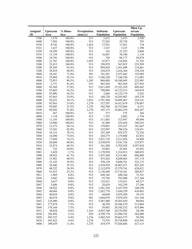
121

Assigned ID

Upstream Area

% Hima-laya

Precipitation (mm/yr)

Subbasin Population

Upstream Population

50km Up-stream Population

5700 1,570 100.0% 913 2,473 2,473 2,500 5600 7,583 100.0% 913 27,265 29,738 703 5530 8,742 100.0% 1,025 17,921 17,921 734 5522 1,627 100.0% 913 3,167 3,167 1,798 5520 10,399 100.0% 913 165 21,253 5,860 5510 11,138 100.0% 913 16,847 38,100 1,118 5500 18,793 100.0% 913 339 68,177 36,874 5400 21,787 100.0% 1,055 47,877 116,054 31,745 5300 23,415 100.0% 913 250,978 367,032 233,589 5200 29,305 83.4% 913 994,858 1,361,890 118,461 5100 30,410 80.4% 913 254,474 1,616,364 159,224 5000 34,101 71.9% 991 741,281 2,357,645 155,969 4910 35,044 43.1% 913 7,186,320 7,186,320 111,083 4900 72,953 90.3% 1,245 804,680 10,348,645 223,985 4820 2,731 41.6% 913 963,564 963,564 637,943 4800 83,369 37.8% 913 2,011,020 13,323,229 409,442 4700 87,065 36.2% 913 799,084 14,122,313 169,839 4600 87,096 36.2% 913 2,866 14,125,179 2,542 4500 87,865 35.9% 913 168,728 14,293,907 185,278 4400 92,633 34.1% 1,032 1,791,560 16,085,467 354,141 4300 93,963 33.6% 1,278 327,207 16,412,674 270,887 4200 95,003 33.3% 1,278 342,390 16,755,064 4,151 4100 95,036 51.0% 1,278 107,175 16,862,239 445,287 4010 267 100.0% 913 375 375 366 4000 1,134 100.0% 913 1,707 2,082 1,754 3990 11,145 100.0% 913 311,865 313,947 99,494 3980 12,080 100.0% 913 41,489 355,436 109,255 3970 13,373 94.1% 913 179,891 535,327 181,647 3960 15,201 82.9% 913 252,997 788,324 129,451 3950 16,153 78.1% 913 147,249 935,573 72,356 3940 16,690 75.6% 913 244,375 1,179,948 62,852 3930 17,044 74.1% 913 1,031,710 2,211,658 34,489 3920 20,860 60.8% 913 3,330,070 5,541,728 135,937 3910 21,074 60.2% 913 161,200 5,702,928 4,297,010 3902 332 44.0% 913 43,963 43,963 43,452 3901 5,428 2.7% 913 1,170,950 1,214,913 240,819 3900 30,922 41.7% 913 1,297,560 8,215,401 606,888 3895 31,981 40.3% 913 475,202 8,690,603 197,174 3890 33,143 38.9% 913 358,158 9,048,761 523,175 3880 36,446 35.5% 913 1,418,910 10,467,671 825,242 3870 48,252 26.9% 913 2,112,070 12,579,741 620,621 3860 51,633 25.2% 913 1,130,440 13,710,181 309,837 3851 1,969 0.0% 913 648,186 648,186 72,761 3850 2,042 0.0% 913 55,794 703,980 217,244 3848 3,627 0.0% 913 133,631 133,631 49,217 3847 3,686 0.0% 913 28,628 162,259 27,346 3846 24,922 0.0% 919 1,301,320 2,167,559 140,358 3845 40,044 0.0% 919 1,262,770 3,430,329 410,463 3844 40,054 0.0% 913 44,040 3,474,369 39,155 3843 60,674 0.0% 961 1,604,070 5,078,439 161,168 3842 125,990 0.0% 913 5,487,400 10,565,839 80,064 3841 177,874 7.5% 913 30,250 24,306,270 212,064 3840 178,168 7.5% 913 38,962 24,345,232 615,486 3831 44,424 0.0% 1,165 4,925,760 29,270,992 24,188 3830 256,992 5.2% 929 4,709,770 33,980,762 303,080 3820 303,355 4.4% 1,234 5,682,510 39,663,272 58,296 3810 303,422 4.4% 1,278 75,576 39,738,848 410,595 3800 399,639 11.4% 1,278 419,579 57,020,666 427,115

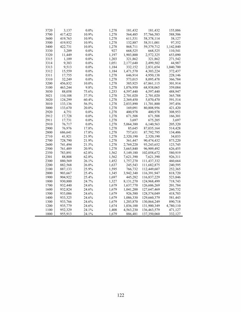
122

3720 3,137 0.0% 1,278 181,432 181,432 155,886 3700 417,422 10.9% 1,278 564,485 57,766,583 588,506 3600 419,763 10.9% 1,278 611,531 58,378,114 38,127 3500 419,932 10.9% 1,278 132,887 58,511,001 97,352 3400 422,731 10.8% 1,278 868,711 59,379,712 1,142,840 3330 3,209 0.0% 927 668,525 668,525 110,541 3320 11,449 0.0% 1,197 1,903,800 2,572,325 653,090 3315 1,109 0.0% 1,203 321,862 321,862 271,542 3314 9,383 0.0% 1,051 2,177,640 2,499,502 44,987 3313 9,513 0.0% 1,184 332,152 2,831,654 1,040,700 3312 15,559 0.0% 1,184 1,471,570 4,303,224 372,437 3311 17,755 0.0% 1,278 646,914 4,950,138 228,146 3310 32,249 0.0% 1,278 573,015 8,095,478 366,784 3200 456,832 10.0% 1,278 385,925 67,861,115 301,914 3100 463,244 9.8% 1,278 1,076,950 68,938,065 359,084 3030 88,058 75.6% 1,253 4,597,440 4,597,440 488,947 3021 110,108 37.5% 1,278 2,701,020 2,701,020 365,788 3020 124,299 60.4% 1,278 2,369,450 5,070,470 591,514 3010 133,136 56.5% 1,278 2,033,890 11,701,800 397,456 3000 133,670 20.0% 1,278 169,091 80,808,956 421,420 2920 4,751 0.0% 1,278 400,978 400,978 308,953 2912 17,728 0.0% 1,278 671,508 671,508 166,301 2911 17,731 0.0% 1,278 3,697 675,205 3,697 2910 76,717 0.0% 1,278 5,064,380 6,140,563 205,320 2900 76,976 17.8% 1,278 85,645 87,035,164 514,428 2800 686,641 17.8% 1,278 757,631 87,792,795 134,406 2710 41,921 21.9% 1,278 2,320,190 2,320,190 34,033 2700 728,790 21.9% 1,278 361,447 90,474,432 873,220 2600 741,494 21.5% 1,278 2,769,220 93,243,652 123,745 2500 761,489 20.9% 1,278 3,665,840 96,909,492 626,455 2350 783,891 62.8% 1,562 5,149,180 102,058,672 580,919 2301 88,808 62.8% 1,562 7,621,390 7,621,390 926,311 2300 880,569 26.1% 1,452 1,757,270 111,437,332 460,664 2200 882,568 26.0% 1,637 245,543 111,682,875 240,595 2100 887,133 25.9% 1,595 766,732 112,449,607 252,365 2000 903,667 25.4% 1,345 3,942,340 116,391,947 818,720 1900 904,922 25.4% 1,697 445,282 116,837,229 523,846 1800 930,800 24.7% 1,327 8,131,270 124,968,499 718,743 1700 932,440 24.6% 1,679 1,637,770 126,606,269 201,784 1600 932,824 24.6% 1,679 1,041,200 127,647,469 260,732 1500 933,086 24.6% 1,679 926,580 128,574,049 418,703 1400 933,325 24.6% 1,679 1,086,330 129,660,379 581,443 1300 933,766 24.6% 1,679 1,203,870 130,864,249 890,718 1200 935,779 24.6% 1,674 1,036,100 131,900,349 4,780,110 1100 952,329 24.1% 1,408 4,563,230 136,463,579 471,127 1000 955,913 24.1% 1,679 886,481 137,350,060 332,127

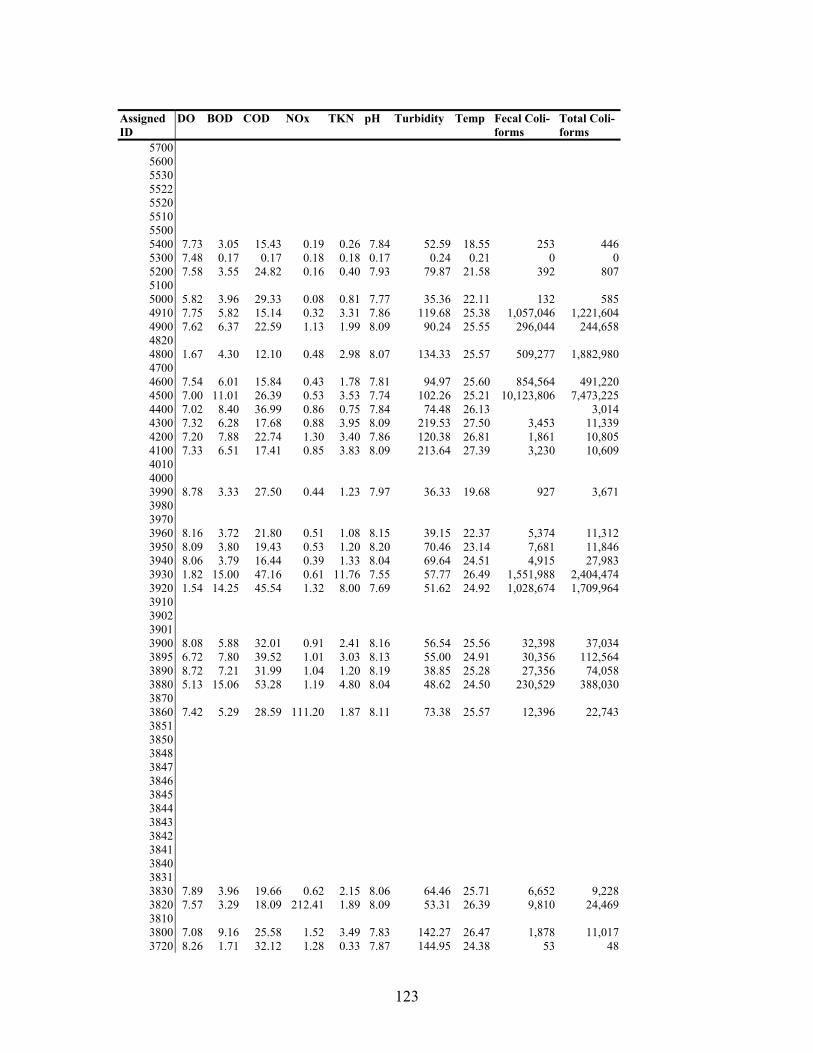
123

Assigned ID

DO BOD COD NOx TKN pH Turbidity Temp Fecal Coli-forms

Total Coli-forms

5700 5600 5530 5522 5520 5510 5500 5400 7.73 3.05 15.43 0.19 0.26 7.84 52.59 18.55 253 446 5300 7.48 0.17 0.17 0.18 0.18 0.17 0.24 0.21 0 0 5200 7.58 3.55 24.82 0.16 0.40 7.93 79.87 21.58 392 807 5100 5000 5.82 3.96 29.33 0.08 0.81 7.77 35.36 22.11 132 585 4910 7.75 5.82 15.14 0.32 3.31 7.86 119.68 25.38 1,057,046 1,221,604 4900 7.62 6.37 22.59 1.13 1.99 8.09 90.24 25.55 296,044 244,658 4820 4800 1.67 4.30 12.10 0.48 2.98 8.07 134.33 25.57 509,277 1,882,980 4700 4600 7.54 6.01 15.84 0.43 1.78 7.81 94.97 25.60 854,564 491,220 4500 7.00 11.01 26.39 0.53 3.53 7.74 102.26 25.21 10,123,806 7,473,225 4400 7.02 8.40 36.99 0.86 0.75 7.84 74.48 26.13 3,014 4300 7.32 6.28 17.68 0.88 3.95 8.09 219.53 27.50 3,453 11,339 4200 7.20 7.88 22.74 1.30 3.40 7.86 120.38 26.81 1,861 10,805 4100 7.33 6.51 17.41 0.85 3.83 8.09 213.64 27.39 3,230 10,609 4010 4000 3990 8.78 3.33 27.50 0.44 1.23 7.97 36.33 19.68 927 3,671 3980 3970 3960 8.16 3.72 21.80 0.51 1.08 8.15 39.15 22.37 5,374 11,312 3950 8.09 3.80 19.43 0.53 1.20 8.20 70.46 23.14 7,681 11,846 3940 8.06 3.79 16.44 0.39 1.33 8.04 69.64 24.51 4,915 27,983 3930 1.82 15.00 47.16 0.61 11.76 7.55 57.77 26.49 1,551,988 2,404,474 3920 1.54 14.25 45.54 1.32 8.00 7.69 51.62 24.92 1,028,674 1,709,964 3910 3902 3901 3900 8.08 5.88 32.01 0.91 2.41 8.16 56.54 25.56 32,398 37,034 3895 6.72 7.80 39.52 1.01 3.03 8.13 55.00 24.91 30,356 112,564 3890 8.72 7.21 31.99 1.04 1.20 8.19 38.85 25.28 27,356 74,058 3880 5.13 15.06 53.28 1.19 4.80 8.04 48.62 24.50 230,529 388,030 3870 3860 7.42 5.29 28.59 111.20 1.87 8.11 73.38 25.57 12,396 22,743 3851 3850 3848 3847 3846 3845 3844 3843 3842 3841 3840 3831 3830 7.89 3.96 19.66 0.62 2.15 8.06 64.46 25.71 6,652 9,228 3820 7.57 3.29 18.09 212.41 1.89 8.09 53.31 26.39 9,810 24,469 3810 3800 7.08 9.16 25.58 1.52 3.49 7.83 142.27 26.47 1,878 11,017 3720 8.26 1.71 32.12 1.28 0.33 7.87 144.95 24.38 53 48

124

3700 6.94 6.60 22.34 1.02 3.90 8.06 153.04 28.19 2,828 12,029 3600 7.05 9.16 25.80 0.83 4.04 7.92 107.93 26.57 1,795 7,328 3500 3400 7.07 8.67 25.84 0.98 3.50 7.99 112.11 27.91 1,538 5,437 3330 3320 3315 3314 3313 3312 8.10 1.51 17.58 7.89 424.88 25.88 3,214 11,045 3311 3310 3200 8.29 9.31 25.75 1.11 3.09 7.98 106.61 26.25 1,756 7,114 3100 7.74 1.68 19.70 2.65 0.51 7.80 270.61 25.72 5,816 34,969 3030 3021 3020 3010 7.92 1.48 18.18 0.47 7.98 254.00 26.20 1,588 7,223 3000 2920 8.44 2.16 30.84 0.28 0.52 8.02 338.65 24.59 23 38 2912 2911 2910 8.06 1.79 20.00 0.82 7.70 286.90 25.42 2,864 13,895 2900 2800 7.77 1.81 21.02 8.60 2.14 7.84 306.07 26.29 11,465 53,695 2710 2700 7.72 1.86 23.17 7.83 310.24 26.80 15,417 60,101 2600 7.86 1.52 18.89 7.86 301.39 26.07 1,494 6,748 2500 7.82 2.21 21.09 7.88 326.43 25.64 2,714 10,495 2350 7.72 1.43 17.38 7.95 247.44 25.03 4,929 9,230 2301 2300 7.87 1.51 21.01 7.82 259.81 26.21 5,846 22,258 2200 7.89 0.79 13.60 0.09 0.46 8.04 292.73 25.64 26,969 66,425 2100 7.61 1.10 15.50 0.10 1.37 8.13 292.43 24.47 14,520 33,621 2000 7.24 1.04 13.08 0.14 0.34 8.07 250.39 26.46 36,043 83,908 1900 7.19 1.24 14.70 1.37 0.38 8.09 251.61 26.40 38,698 50,395 1800 7.01 1.64 19.56 0.09 0.37 8.02 230.60 25.60 33,522 86,945 1700 7.12 1.49 17.90 0.13 1.69 8.05 238.25 25.02 54,572 125,690 1600 1500 6.94 3.09 24.67 0.13 2.11 8.08 253.92 25.19 101,258 203,716 1400 1300 1200 6.58 1.91 19.25 0.15 1.98 8.03 256.94 25.13 93,973 190,464 1100 1000 6.69 11.13 126.42 0.37 0.47 7.98 393.21 26.35 29,023 40,649

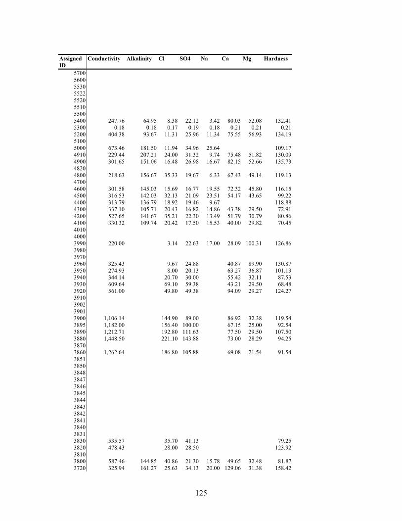
125

Assigned ID

Conductivity Alkalinity Cl SO4 Na Ca Mg Hardness

5700 5600 5530 5522 5520 5510 5500 5400 247.76 64.95 8.38 22.12 3.42 80.03 52.08 132.41 5300 0.18 0.18 0.17 0.19 0.18 0.21 0.21 0.21 5200 404.38 93.67 11.31 25.96 11.34 75.55 56.93 134.19 5100 5000 673.46 181.50 11.94 34.96 25.64 109.17 4910 229.44 207.21 24.00 31.32 9.74 75.48 51.82 130.09 4900 301.65 151.06 16.48 26.98 16.67 82.15 52.66 135.73 4820 4800 218.63 156.67 35.33 19.67 6.33 67.43 49.14 119.13 4700 4600 301.58 145.03 15.69 16.77 19.55 72.32 45.80 116.15 4500 316.53 142.03 32.13 21.09 23.51 54.17 43.65 99.22 4400 313.79 136.79 18.92 19.46 9.67 118.88 4300 337.10 105.71 20.43 16.82 14.86 43.38 29.50 72.91 4200 527.65 141.67 35.21 22.30 13.49 51.79 30.79 80.86 4100 330.32 109.74 20.42 17.50 15.53 40.00 29.82 70.45 4010 4000 3990 220.00 3.14 22.63 17.00 28.09 100.31 126.86 3980 3970 3960 325.43 9.67 24.88 40.87 89.90 130.87 3950 274.93 8.00 20.13 63.27 36.87 101.13 3940 344.14 20.70 30.00 55.42 32.11 87.53 3930 609.64 69.10 59.38 43.21 29.50 68.48 3920 561.00 49.80 49.38 94.09 29.27 124.27 3910 3902 3901 3900 1,106.14 144.90 89.00 86.92 32.38 119.54 3895 1,182.00 156.40 100.00 67.15 25.00 92.54 3890 1,212.71 192.80 111.63 77.50 29.50 107.50 3880 1,448.50 221.10 143.88 73.00 28.29 94.25 3870 3860 1,262.64 186.80 105.88 69.08 21.54 91.54 3851 3850 3848 3847 3846 3845 3844 3843 3842 3841 3840 3831 3830 535.57 35.70 41.13 79.25 3820 478.43 28.00 28.50 123.92 3810 3800 587.46 144.85 40.86 21.30 15.78 49.65 32.48 81.87 3720 325.94 161.27 25.63 34.13 20.00 129.06 31.38 158.42

126

3700 379.41 140.11 28.70 16.65 17.90 55.00 37.40 92.40 3600 483.55 156.20 44.41 19.94 14.19 66.63 57.87 123.43 3500 3400 475.73 150.68 47.11 21.61 16.35 128.40 10.81 138.25 3330 3320 3315 3314 3313 3312 377.79 145.00 15.92 15.43 18.43 71.00 230.50 3311 3310 3200 468.48 155.05 44.71 21.64 13.44 120.46 20.23 141.00 3100 313.82 150.45 21.99 17.72 17.18 114.53 30.59 143.56 3030 3021 3020 3010 29.40 104.84 8.40 11.00 12.60 88.50 44.00 132.50 3000 2920 227.31 123.43 24.58 30.00 16.60 119.72 2912 2911 2910 174.25 91.18 11.25 10.53 13.05 80.51 59.35 139.43 2900 2800 275.33 132.22 15.82 15.84 19.65 80.75 61.08 142.95 2710 2700 283.60 133.13 15.49 15.04 21.12 70.12 45.47 331.40 2600 357.94 135.10 14.60 15.16 26.44 230.33 2500 367.71 142.64 14.69 14.16 18.29 117.32 212.61 322.06 2350 370.07 141.92 14.30 15.11 16.50 87.61 48.57 136.18 2301 2300 262.38 129.80 14.67 14.13 16.13 79.37 53.38 132.54 2200 361.27 114.76 9.38 20.06 11.97 243.13 2100 282.85 108.58 9.88 15.86 13.09 77.38 43.84 123.47 2000 289.21 122.88 9.21 21.19 13.84 369.30 1900 305.88 123.36 9.36 21.00 10.97 195.86 1800 307.18 125.59 9.60 20.76 10.84 77.24 52.54 125.04 1700 292.05 111.46 11.96 16.75 12.09 74.31 59.91 133.96 1600 1500 318.36 113.49 13.44 19.80 14.08 75.57 45.95 121.82 1400 1300 1200 310.11 110.79 15.38 18.57 15.36 70.87 53.94 124.13 1100 1000 3,285.36 115.22 701.53 171.91 739.30 79.53 61.47 141.00