Modeling the Dynamic Evolution of the Solar Atmosphere:

C4: HMI-AIA Team Meeting: 2-14-06

Bill Abbett

SSL, UC Berkeley

Among the AIA’s stated objectives:

• “To understand the evolution of the coronal magnetic field toward unstable configurations by stresses induced at the solar surface”

Ultimately, we must understand the dynamic magnetic and energetic connection between the photosphere and corona.

Available theoretical / computational tools:1. Sequences of static / steady-state models

2. Dynamic MHD models of the solar atmosphere

1. Sequences of static/steady-state models:

Measure the magnetic field at the photosphere (and/or chromosphere)

perform global (or local) potential field and/or non-constant-α force-free extrapolations

construct steady-state solutions to the continuity, momentum, and energy equations along selected fieldlines

generate synthetic images using known instrumental bandpasses

directly compare with observations

interpret the results (e.g., understand helicity transport, energetics, topological changes), and place further observational constraints on the models

Example: Lundquist 2006:

AR 8210 (CME producing AR)

Extrapolation: optimization technique (Wheatland et al. 2000)

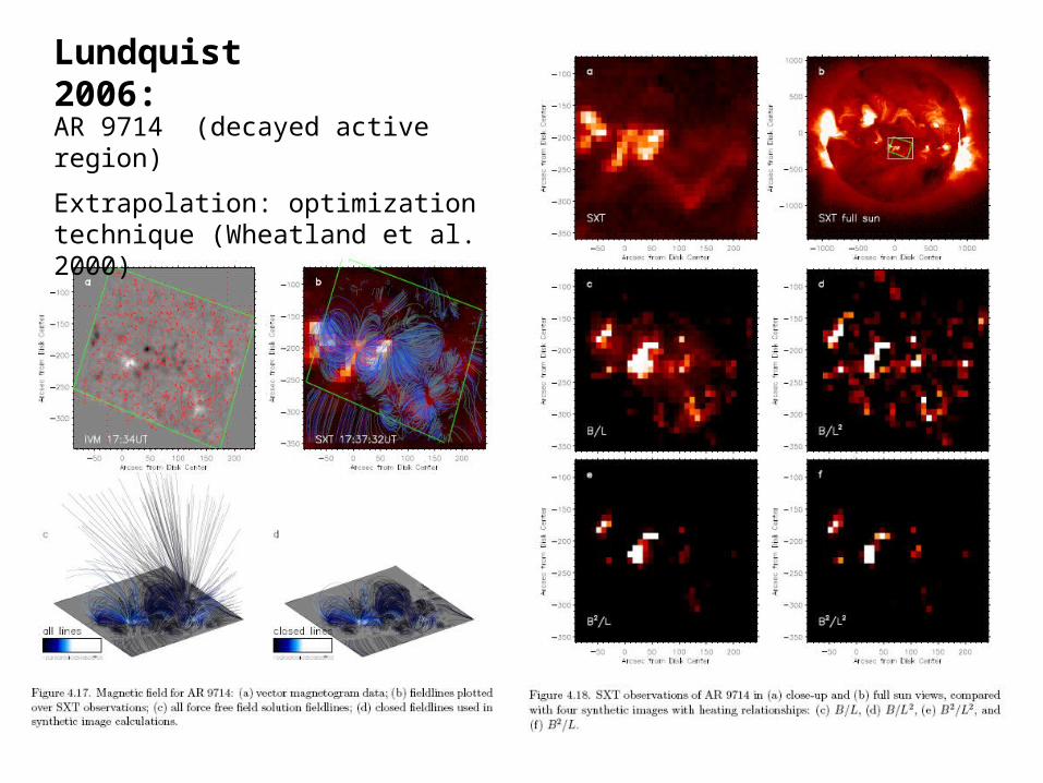
Lundquist 2006:

AR 9714 (decayed active region)

Extrapolation: optimization technique (Wheatland et al. 2000)

Interpreting steady state models

Suppose we wish to understand the buildup and release of freemagnetic energy in the solar corona in and around a particular active region complex.

Q: When are dynamic models necessary, and when are static descriptions sufficient?

Put another way:

Q: When is the history of the magnetic field necessary to properly describe the magnetic topology of the corona?

– Is all the necessary information contained in the vector magnetic field along the boundaries?

– If we assume ideal MHD evolution, is there a unique topology associated with a given set of boundary conditions? What if changes in magnetic topology occur as a result of reconnection?

– When should we worry about the non-uniqueness of the non-linear force-free extrapolation?

Consider the following …

• extreme spatial and temporal disparities– small-scale, active region, and global features are fundamentally

inter-connected – magnetic features at the photosphere are long-lived (relative to

the convective turnover time) while features in the magnetized corona can evolve rapidly (e.g., topological changes following reconnection events)

• different physical regimes– photosphere and below: relatively dense, turbulent (high-β)

plasma with strong magnetic fields organized in isolated structures

– corona: field-filled, low-density, magnetically dominated plasma (at least around strong concentrations of magnetic flux!)

– flow speeds in CZ below the surface are typically below the characteristic sound and Alfven speeds, while the chromosphere, transition region and corona are often shock-dominated

2. Dynamic models: some realities

• different physical regimes (cont’d)– corona: energetics dominated by optically thin radiative cooling,

anisotropic thermal conduction, and some form of coronal heating consistent with the empirical relationship of Pevtsov et al. 2003 (energy dissipation as measured by soft X-rays proportional to the measured unsigned magnetic flux at the photosphere)

– photosphere/chromosphere: energetics dominated by optically thick radiative transitions

Additional computational challenges:• A dynamic model atmosphere extending from below the photosphere

to the corona must:– span a ~10 order of magnitude change in gas density and a

thermodynamic transition from the 1MK corona to the optically thick, cooler layers of the low atmosphere, visible surface, and below

– resolve a ~100km photospheric pressure scale height (energy scale height in the transition region can be as small as 1km!) while following large-scale evolution

What’s out there?

A number of numerical codes are publicly available, each designed to efficiently describe the physics of a specific regime, at various spatial and temporal scales.

What’s missing?

Robust efficient codes that treat both the magnetic and energetic transition between the surface layers and corona over large spatial scalesWhat’s missing?

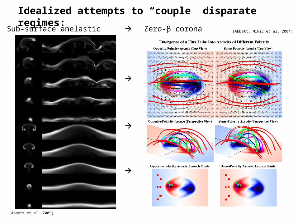
Idealized attempts to “couple” disparate regimes:

Sub-surface anelastic Zero-β corona

(Abbett et al. 2005)

(Abbett, Mikic et al. 2004)

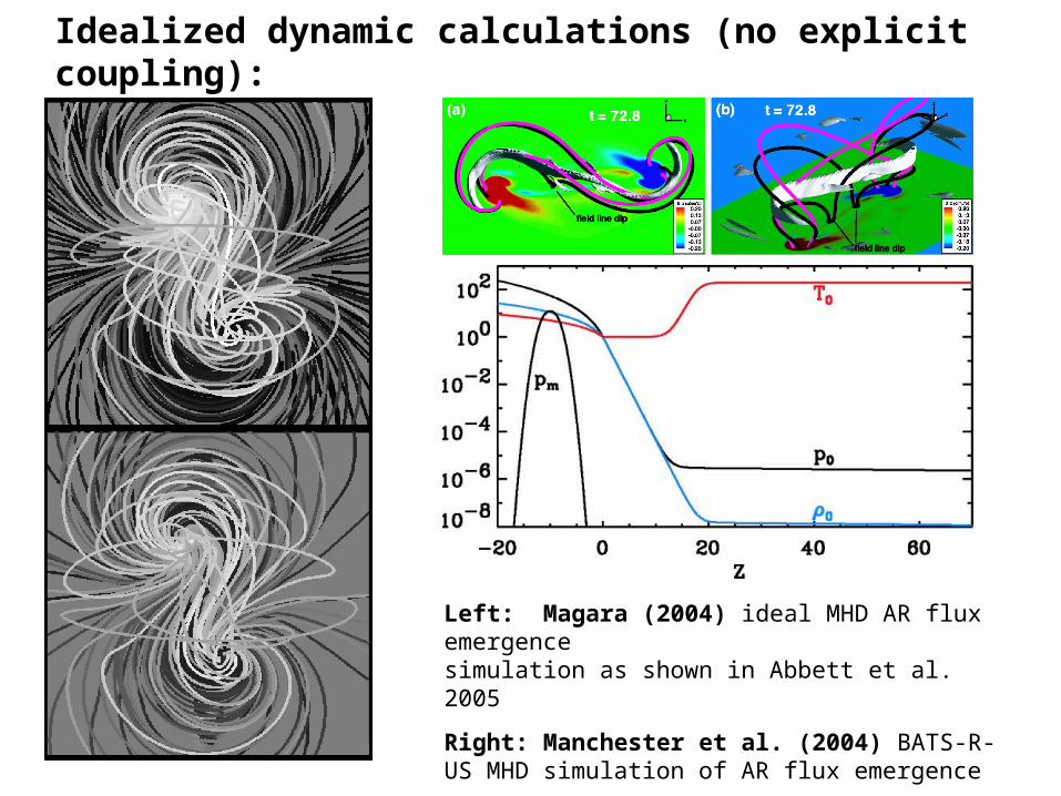
Idealized dynamic calculations (no explicit coupling):

Left: Magara (2004) ideal MHD AR flux emergence simulation as shown in Abbett et al. 2005

Right: Manchester et al. (2004) BATS-R-US MHD simulation of AR flux emergence

A qualitative comparison:

potential field MHDNon-linear force-free

Toward more realistic AR models:

We must solve the following system:

Energy source terms (Q) include:

• Optically thin radiative cooling

• Anisotropic thermal conduction

• An option for an empirically-based coronal heating mechanism --- must maintain a corona consistent with the empirical constraint of Pevtsov (2003)

• LTE optically thick cooling (options: solve the grey transfer equation in the 3D Eddington approximation, or use a simple parameterization that maintains the super-adiabatic gradient necessary to initiate and maintain convective turbulence)

Surmounting practical computational challenges

• The MHD system is solved semi-implicitly on a block adaptive mesh.

• The non-linear portion of the system is treated explicitly using the semi-discrete central method of Kurganov-Levy (2000) using a 3rd-order CWENO polynomial reconstruction

– Provides an efficient shock capture scheme, AMR is not required to resolve shocks

• The implicit portion of the system, the contributions of the energy source terms, and the resistive and viscous contributions to the induction and momentum equations respectively, is solved via a “Jacobian-free” Newton-Krylov technique

– Makes it possible to treat the system implicitly (thereby providing a means to deal with temporal disparities) without prohibitive memory constraints

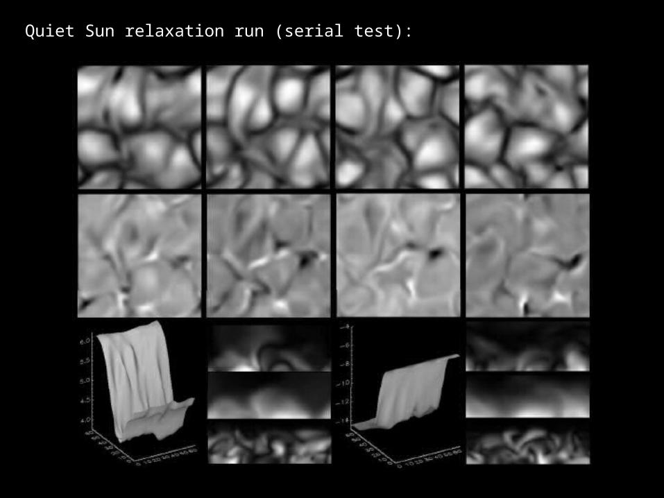
Quiet Sun relaxation run (serial test):

Toward AR scale: MPI-AMR relaxation run (test)

The near-term plan:

• Dynamically and energetically relax a 30Mm square Cartesian domain extending to ~2.5Mm below the surface.

• Introduce a highly-twisted AR-scale magnetic flux rope (from the top of a sub-surface calculation) through the bottom boundary of the domain

• Reproduce (hopefully!) a highly sheared, δ-spot type AR at the surface, and follow the evolution of the model corona as AR flux emerges into, reconnects and reconfigures coronal fields

The long term plan:

• global scales / spherical geometery

Q: How do different treatments of the coefficient of resistivity, or changes in resolution affect the topological evolution of the corona?

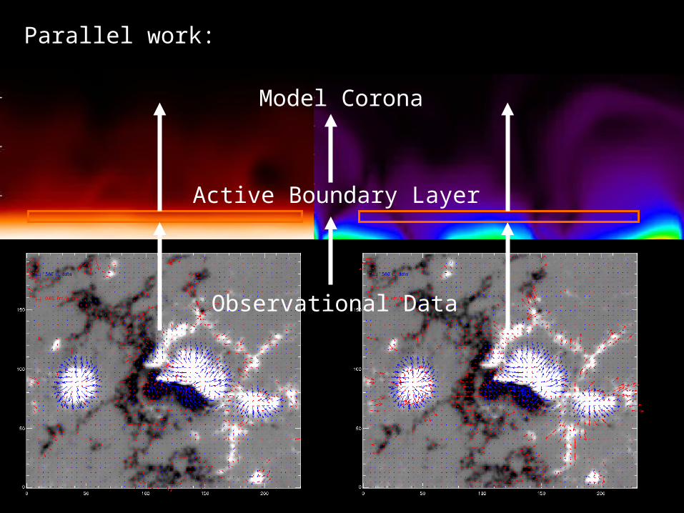
Parallel work:

Observational Data

Active Boundary Layer

Model Corona

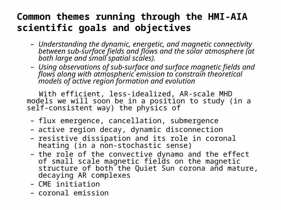
– Understanding the dynamic, energetic, and magnetic connectivity between sub-surface fields and flows and the solar atmosphere (at both large and small spatial scales).

– Using observations of sub-surface and surface magnetic fields and flows along with atmospheric emission to constrain theoretical models of active region formation and evolution

With efficient, less-idealized, AR-scale MHD models we will soon be in a position to study (in a self-consistent way) the physics of

– flux emergence, cancellation, submergence– active region decay, dynamic disconnection– resistive dissipation and its role in coronal heating (in a non-

stochastic sense)– the role of the convective dynamo and the effect of small scale

magnetic fields on the magnetic structure of both the Quiet Sun corona and mature, decaying AR complexes

– CME initiation– coronal emission

Common themes running through the HMI-AIA scientific goals and objectives