Arterial Oxygen Saturation in Children Following General ...
Modeling the Dependency of Oxygen Saturation Levels in Tissue on the Blood Flow of
Capillary Units
University of Western Ontario
Department of Medical Biophysics
Ryan Divigalpitiya
Supervisor: Dr. Dan Goldman
1
Table of Contents
1 - Introduction! 1.1 - Motivation for a Model that Predicts Oxygen Saturation2 - Background! 2.1 - Biological Background! ! 2.1.1 - Microvasculature! ! 2.1.2 - Blood Properties! 2.2 - Basic Modeling! 2.3 - Background on Ellsworth et alʼs research “Measurement of Hemoglobin Oxygen Saturation in Capillaries”3 - Objectives4 - Methods & Approach! 4.1 - Components of MATLAB Model! ! 4.1.1 - Geometry! ! 4.1.2 - Tissue Properties! ! 4.1.3 - Incorporating the Saturation Equation5 - Results! 5.1 - Contour Plots! 5.2 - Finite Sensitivity! 5.3 - Resolution6 - Discussion! 6.1 - Is this Basic Model Working?! 6.2 - Finite Sensitivity! 6.3 - Resolution! 6.4 - Future Ideas7 - Conclusion7 - References
2

Acknowledgements
I would like to thank Dr. Dan Goldman, my supervisor, who was involved with the project
and provided the much needed guidance and help I needed. It has been a great
learning experience.
Ryan Divigalpitiya,
April, 2011
3

1 - Introduction! Oxygen is one of the few elements human beings require constantly in order to
survive longer than a few minutes. With such a critical dependency on oxygen, diseases
that restrict or interfere with oxygen delivery throughout our body pose immediate
dangers to our short term health. This has been a platform of motivation to increase our
understanding of the dynamics of oxygen transport and oxygen levels in the body.
! When dealing with a more local scenario of de-oxygenation such as necrosis in
tissue, how researchers can gauge levels of oxygen is by measuring a property known
as oxygen saturation in tissue. Necrosis occurs when oxygen saturation levels have
been zero for too long and the tissue has started to die. There are various diseases that
exhibit these kind of results as their symptoms such as Sepsis or Systemic
Inflammatory Response Syndrome (SIRS).
1.1 - Motivation for a Model that Predicts Oxygen Saturation
! If we are able to create a software model that can predict the oxygen saturation
levels in various tissue under various states, we would not only be able to broaden our
understanding of the dynamics of oxygen saturation but, more significantly, we could
utilize such a model to aid us in revealing treatments and cures for diseases like sepsis
that we were unable to see before. This vision is a vision of the ultimate goal of what I
want to achieve with this project but I will outline further on why its more wise to
consider modeling a simpler case first.
4
2 - Background2.1 - Biological Background
2.1.1 - Microvasculature
! The primary site of oxygen diffusion into the tissue occurs at the microvascular
sites known as the capillaries. Here, red blood cells usually travel one at a time from the
inlet of the capillary to the outlet and release their oxygen molecules along the way. The
dimensions of an average capillary is roughly about 6 - 8 μm in diameter where a red
blood cell is also roughly about 6-8 μm in diameter1. The shape of a capillary is
essentially cylindrical.
2.1.2 - Blood Properties
! Red blood cells are the carriers of oxygen throughout the microvasculature.
However, they require the help of a protein molecule in order to sufficiently bind enough
oxygen molecules to be transported in the blood. This protein is called Hemoglobin and
is an iron-containing, multi-subunit protein that makes up 97% of a red blood cells dry
content2. It is generally found in two states. 1) Saturated - the Hemoglobin is bounded to
oxygen, 2) Unsaturated - the Hemoglobin is unbounded to oxygen.
! This is effectively what oxygen saturation in tissue is based on - if we can
measure the amount of hemoglobin with bounded oxygen, we know the oxygen
saturation at that point in the tissue.
! Another important and relevant tissue property is Hematocrit. Hematocrit is the
fraction of blood volume occupied by red blood cells. The rest of the blood is occupied
by other species such as blood plasma.
5

2.2 - Basic Modeling
! Before one attempts to model complex scenarios that reflect diseases and
illnesses, itʼs wise to first attempt to model the simplest scenario first and see if doing so
is feasible. Once successful, then we are in a position to generate ideas for the next,
more complicated revision of the model.
! So how did I define what entails a simple model? First, I eliminated diseases
altogether and decided to model “healthy” tissue (tissue with no disease). I also limited
the microvasculature to one single capillary in my healthy tissue because, otherwise,
modeling an entire capillary network would have been another substantial source of
complexity to worry about.
! Next, I considered what my input and output were going to be in the context of
this project. The input has to be some measured tissue property thatʼs related to the
oxygen saturation. The output will be mean oxygen saturation levels. The computational
algorithm that computes the saturation based on the input was essentially what I had to
determine for this project. To help me with this part I based the algorithm on research
conducted by Ellsworth et al3.
2.3 - Background on Ellsworth et alʼs research “Measurement of Hemoglobin
Oxygen Saturation in Capillaries”3
! Ellsworth et al conducted research on determining oxygen saturation in tissue by
measuring the optical densities of the tissue. Essentially, they shined specific
wavelengths of light through tissue and used a detector to measure the transmitted light
intensity. The wavelength were selected based on the absorption spectra of
6

hemoglobin. Using the Optical Density equation (OD) which equals Log(I/Io) where I =
transmitted intensity, and Io = initial intensity, the OD was calculated for the tissue at that
specific point in the tissue. Since, the measured OD is the OD of hemoglobin which can
then be correlated to the saturation levels in the capillaries, Ellsworth et al managed to
express the relationship between optical density and oxygen saturation in this equation:
! This Saturation Equation was selected to be the heart of the modelʼs
computational algorithm. It would be incorporated into the model such that, one would
only have to measure the optical density of the tissue of interest once, input the values
into model and model should be able to estimate the saturation of oxygen everywhere
else in the tissue.
! Thus, what this means is that the estimation of the saturation is dependent on the
limitations of the equipment used to make that initial optical density measurement.
Certain parameters for the equipment may limit the accuracy of the saturation
estimation. One very important parameter, called the Finite Sensitivity of the detector,
which is a measure of the minimum intensity of light the detector can detect, could be a
limiting factor in the accuracy of modeling the saturation levels. The choice of finite
sensitivity in the detector we use may be influenced by the tissue properties in the
tissue of interest and would, thus, be interesting to investigate if there are any
connections between the two. Also, very common in models of this nature, is the impact
of selecting an appropriate “resolution” to run the model at. Too high a resolution would
cause the model to take a long duration of time to compute the answer but may reveal a
S = -1.56*(OD431/OD420)+1.78
7

very accurate answer and vice versa. It would also be interesting to investigate if there
are any relationships between the selected resolution and limitations of finite sensitivity
of the detector used.
3 - ObjectivesWith that said, my objectives for this project are the following:
To create a software computational model that accurately predicts mean O2 tissue saturation based on the Saturation Equation
A. Use the model to determine how simulated hematocrit levels affect the required finite sensitivity needed to accurately predict mean saturation
B. Use the model to determine how resolution of the model (the size of the voxels that make up the 3D tissue) affect the accuracy of predicting the required finite sensitivity
C. Use what was learned in creating this simplified model to generate ideas on how to improve the model in an attempt to improve its realism and applicability
4 - Methods & Approach
! The software package that was utilized is called MATLAB which is a matrix-
driven program used in a wide variety of applications.
4.1 - Components of MATLAB Model:
4.1.1 - Geometry
! To create the geometry of the model, I constructed 3D matrixes to the
dimensions of a rectangular prism of 25 μm by 25 μm by 200 μm. I then defined a
cylinder inside this tissue with the same depth of 200 μm and a radius of 3 μm (6 μm
diameter). This cylinder represented the idealized capillary inside the healthy tissue.
8

4.1.2 - Tissue Properties
! The next step was to simulate the relevant tissue properties. Hemoglobin
concentrations were simulated by assuming a hemoglobin concentration of 20 mmol/L
inside every red blood cell3. Hematocrit levels were simulated by assuming levels
between 0.3 and 0.5 which I arbitrarily selected based off common reported values in
the literature. Once, hemoglobin and hematocrit levels were incorporated, I made a
simplified assumption that the saturation would decrease linearly as the blood moves
along the capillary. That way, I could verify myself if the code is functioning properly
because I would be able to independently calculate what the predicted answer should
be and compare it to the modelʼs answer. Another simplification I made was to neglect
red blood cell flow velocity.
4.1.3 - Incorporating the Saturation Equation
! The final step was incorporating the Saturation Equation into the model. It was
incorporated by first calculating all the individual OD431 and OD420 using Beer-Lambertʼs
law: conc x L x e, where concentration, in this context, would be the concentration of
hemoglobin multiplied by the hematocrit; L is the thickness of the capillary (the
diameter); and e is the extinction coefficient of hemoglobin at either OD431 or OD420
depending on which one is being calculated. Then, assuming the saturation is linearly
decreasing, the model would use the Saturation Equation to estimate the mean
saturation of the entire tissue. However, after I preliminarily tested it out, there were
some errors in the calculated saturation - the calculated saturation was always 2
9

decimals off from the “correct” answer. For example, if I knew the calculated saturation
should be 0.5, the model would calculate 0.4522. I soon realized that the extinction
coefficients I was using were reported in the literature with an error range as follows: for
the 420-nm filter, 120.0 ± 8.7 and 112.6 ± 8.3 and for the 431-nm filter they were 62.8 ±
5.0 and 136.7 ± 8.1. After discovering the error ranges, I varied the extinction
coefficients within these ranges until the model computed an answer of 0.5000. Thus, I
optimized the coefficients which improved the accuracy to an acceptable level.
! As I started to achieve a stable and accurate model, I ran my model against my
objectives and collected the outputted results.
10
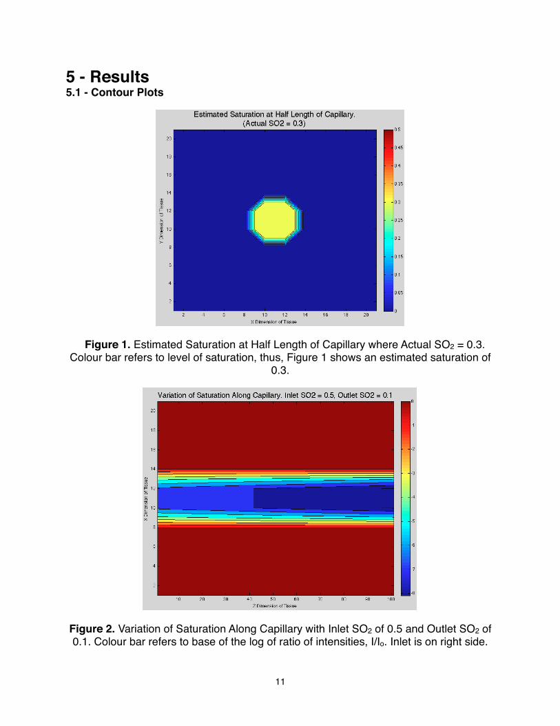
5 - Results5.1 - Contour Plots
Figure 1. Estimated Saturation at Half Length of Capillary where Actual SO2 = 0.3. Colour bar refers to level of saturation, thus, Figure 1 shows an estimated saturation of
0.3.
Figure 2. Variation of Saturation Along Capillary with Inlet SO2 of 0.5 and Outlet SO2 of 0.1. Colour bar refers to base of the log of ratio of intensities, I/Io. Inlet is on right side.
11

Figure 3. Estimated Saturation at Half Length of Capillary where Actual SO2 = 0.5.Colour bar refers to level of saturation, thus, Figure 1 shows an estimated saturation of
0.5.
Figure 4. Variation of Saturation Along Capillary with Inlet SO2 of 0.8 and Outlet SO2 of 0.2. Colour bar refers to base of the log of ratio of intensities, I/Io. Inlet is on right side.
12

! In order to generate these results, inlet and outlet values of saturation were
inputed into the model. With these inputs, the model calculated and estimated the
saturation throughout the modeled tissue where Figures 1 through 4 display these
outputted saturation estimates.
! Figure 1 displays a circular cross section of the modeled capillary. The figure is
not entirely circular due to selection of resolution and artifacts in the generated figure
(however, the artifacts are not interfering with what is being shown). By observing figure
1ʼs colour bar, we can see that the model has estimated the saturation level to be about
0.3 at the half way point along the capillary.
! Figure 2 displays a cylindrical cross section of the modeled capillary where the
figure succeeds to show that the variation in saturation along the capillary can be
observed as decreasing from the inlet toward the outlet. The colour bar reference is
presented using the base of the log of ratio of intensities, I/Io. How one reads the color
bar is as follows. A small value (ie. approaching 0) for the ratio of I/Io indicates high
absorbance ie. high saturation at that point along the capillary. Also, a small value for
the ratio of I/Io indicates larger negative numbers on the colour scale, for example, -6 or
-7 as oppose to -1 or -2. Thus, larger negative numbers on the colour bar indicate
higher saturation, or rather, darker blue colours indicate high saturation and lighter blue
colours indicate lower saturation. This makes sense since the inlet is on the right side of
the figure, has the highest saturation and, thus, has the darkest colour. Figures 3 and 4
are two more similar examples with different inputted values.
13
5.2 - Finite Sensitivity
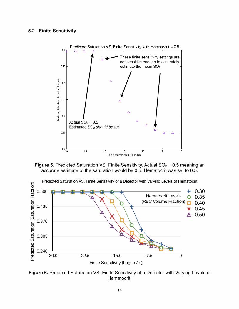
Figure 5. Predicted Saturation VS. Finite Sensitivity. Actual SO2 = 0.5 meaning an accurate estimate of the saturation would be 0.5. Hematocrit was set to 0.5.
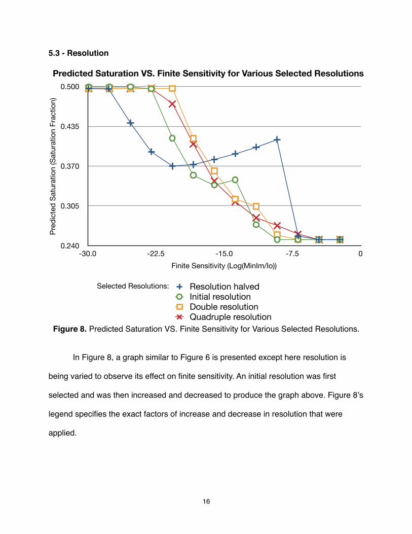
Predicted Saturation VS. Finite Sensitivity of a Detector with Varying Levels of Hematocrit
Figure 6. Predicted Saturation VS. Finite Sensitivity of a Detector with Varying Levels of Hematocrit.
0.240
0.305
0.370
0.435
0.500
-30.0 -22.5 -15.0 -7.5 0
Pre
dic
ted
Sat
urat
ion
(Sat
urat
ion
Frac
tion)
Finite Sensitivity (Log(Im/Io))
0.300.350.400.450.50
14
Actual SO2 = 0.5Estimated SO2 should be 0.5
Hematocrit Levels(RBC Volume Fraction)
These finite sensitivity settings are not sensitive enough to accurately estimate the mean SO2

! The x-axis on both Figure 5 and 6 again use the base of the log of the ratio of
intensities I/Io. Thus, values to the left of the x-axis indicate high finite sensitivity. Values
to the right of the x-axis indicate low finite sensitivity. To determine the effect of
hematocrit levels on finite sensitivity, values within the range of 0.3 to 0.5 hematocrit
were inputted in the model and resulting figure, figure 6, was outputted. It is observed
that the higher the level of hematocrit present in the tissue, a higher finite sensitivity is
required to detect the transmitted intensity in order to accurately predict mean SO2. To
further bring out this trend, the data points corresponding to the point right before each
curve starts to decrease (ie. become inaccurate) was plotted against the increase in
hematocrit levels:
Figure 7. Required Finite Sensitivity for Specified Hematocrit Levels
-24
-21
-18
-15
-12
0.30 0.35 0.40 0.45 0.50
Required Finite Sensitivity for Specified Hematocrit Levels
Req
uire
d F
inite
Sen
sitiv
ity (L
og(Im
/Io)
)
Hematocrit (RBC Volume Fraction)
15
5.3 - Resolution
0.240
0.305
0.370
0.435
0.500
-30.0 -22.5 -15.0 -7.5 0
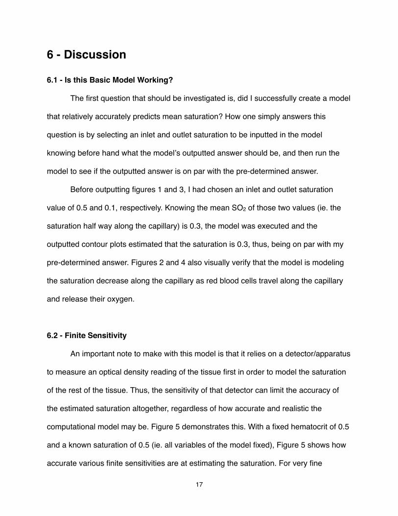
Predicted Saturation VS. Finite Sensitivity for Various Selected Resolutions
Pre
dic
ted
Sat
urat
ion
(Sat
urat
ion
Frac
tion)
Finite Sensitivity (Log(MinIm/Io))
Resolution halvedInitial resolution Double resolutionQuadruple resolution
Figure 8. Predicted Saturation VS. Finite Sensitivity for Various Selected Resolutions. !
! In Figure 8, a graph similar to Figure 6 is presented except here resolution is
being varied to observe its effect on finite sensitivity. An initial resolution was first
selected and was then increased and decreased to produce the graph above. Figure 8ʼs
legend specifies the exact factors of increase and decrease in resolution that were
applied.
16
Selected Resolutions:
6 - Discussion
6.1 - Is this Basic Model Working?
! The first question that should be investigated is, did I successfully create a model
that relatively accurately predicts mean saturation? How one simply answers this
question is by selecting an inlet and outlet saturation to be inputted in the model
knowing before hand what the modelʼs outputted answer should be, and then run the
model to see if the outputted answer is on par with the pre-determined answer.
! Before outputting figures 1 and 3, I had chosen an inlet and outlet saturation
value of 0.5 and 0.1, respectively. Knowing the mean SO2 of those two values (ie. the
saturation half way along the capillary) is 0.3, the model was executed and the
outputted contour plots estimated that the saturation is 0.3, thus, being on par with my
pre-determined answer. Figures 2 and 4 also visually verify that the model is modeling
the saturation decrease along the capillary as red blood cells travel along the capillary
and release their oxygen.
6.2 - Finite Sensitivity
! An important note to make with this model is that it relies on a detector/apparatus
to measure an optical density reading of the tissue first in order to model the saturation
of the rest of the tissue. Thus, the sensitivity of that detector can limit the accuracy of
the estimated saturation altogether, regardless of how accurate and realistic the
computational model may be. Figure 5 demonstrates this. With a fixed hematocrit of 0.5
and a known saturation of 0.5 (ie. all variables of the model fixed), Figure 5 shows how
accurate various finite sensitivities are at estimating the saturation. For very fine
17
sensitivities (ie. detectors that can detect very small intensities of transmitted light), an
accurate estimate of 0.5 saturation is achieved. For courser sensitivities (ie. detectors
that cannot detect very small intensities, only large intensities of transmitted light), the
curve experiences a quick drop which indicates a significant amount of error being
introduced in the estimation as the finite sensitivity worsens (moving towards the right of
the x-axis). This intuitively makes sense since a detector that only has the ability to
detect transmitted minimum intensities of, say, X and then a transmitted intensity of Y
strikes this detector where Y < X, the signal noise and system noise in the detector
would be larger than the detected signal, thus, meaning it would never be detected.
! Figures 6 and 7 go on to investigate the question “what properties of the tissue
affects finite sensitivity?”. ! Figures 6 and 7 clearly demonstrate that as levels of
hematocrit increase in the tissue, a more sensitive detector is required to maintain
accurate estimations of the saturation. Why is this? The answer can be found by
investigating how increasing hematocrit affects the Optical Density equation or Beer-
Lambertʼs law: OD = conc x L x e. An increase in hematocrit simply means an increase
in red blood cells and, thus, hemoglobin. Essentially, there is an increase in
concentration of the species that absorbs the light intensities passing through the tissue.
With increases in the amount of light intensity absorbed, less light is being transmitted
to the detector which, in turn, will require a more sensitive detector to pick up the
diminished transmitted light intensity. Thus, this is why we observe Figure 7ʼs trend: an
increase in hematocrit level requires an increase in the finite sensitivity in order to
maintain an accurate estimation of the saturation because the transmitted intensity gets
weaker.
18
! What we can take away from these findings is that we can actually use the model
to predict for us what finite sensitivity we should be using in our detector in order to
achieve accurate estimations of saturation for specific hematocrit levels.
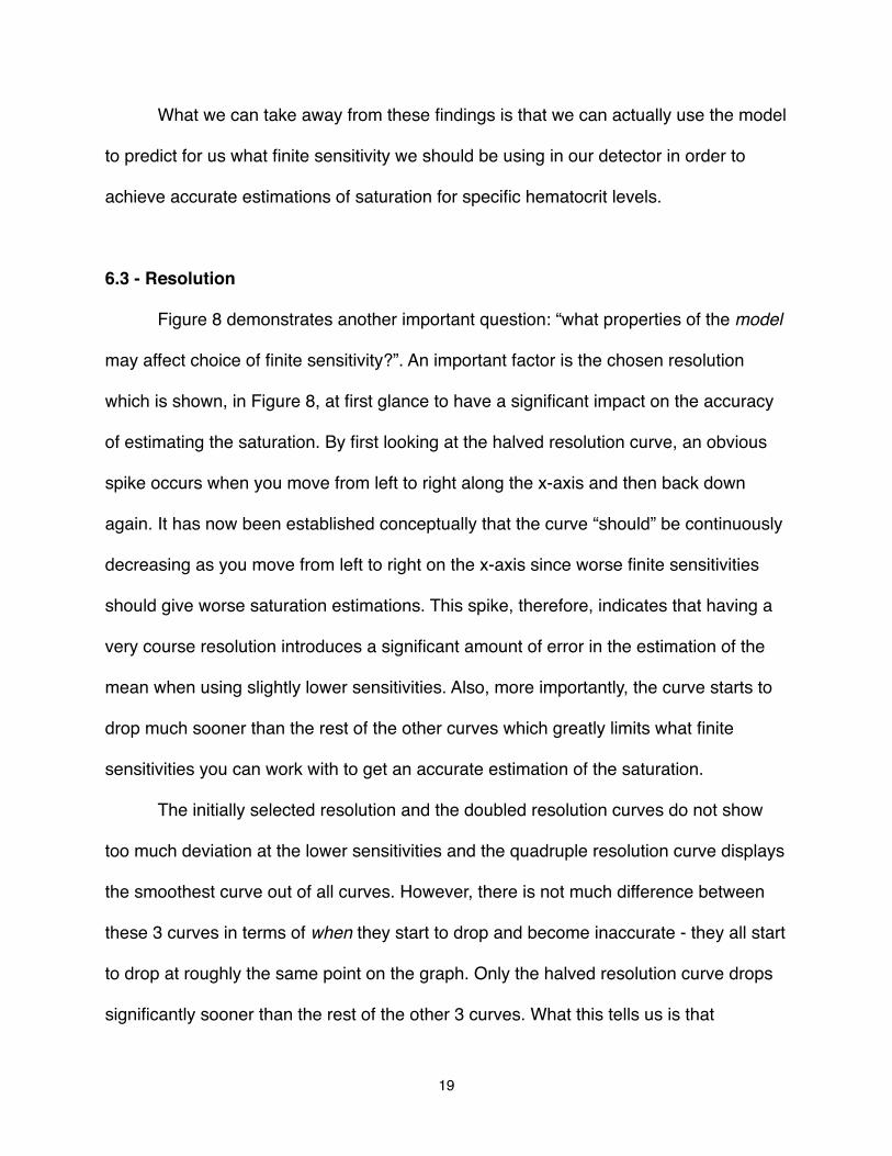
6.3 - Resolution
! Figure 8 demonstrates another important question: “what properties of the model
may affect choice of finite sensitivity?”. An important factor is the chosen resolution
which is shown, in Figure 8, at first glance to have a significant impact on the accuracy
of estimating the saturation. By first looking at the halved resolution curve, an obvious
spike occurs when you move from left to right along the x-axis and then back down
again. It has now been established conceptually that the curve “should” be continuously
decreasing as you move from left to right on the x-axis since worse finite sensitivities
should give worse saturation estimations. This spike, therefore, indicates that having a
very course resolution introduces a significant amount of error in the estimation of the
mean when using slightly lower sensitivities. Also, more importantly, the curve starts to
drop much sooner than the rest of the other curves which greatly limits what finite
sensitivities you can work with to get an accurate estimation of the saturation.
! The initially selected resolution and the doubled resolution curves do not show
too much deviation at the lower sensitivities and the quadruple resolution curve displays
the smoothest curve out of all curves. However, there is not much difference between
these 3 curves in terms of when they start to drop and become inaccurate - they all start
to drop at roughly the same point on the graph. Only the halved resolution curve drops
significantly sooner than the rest of the other 3 curves. What this tells us is that
19

resolution does not play a major role in the accuracy of estimating saturation if you are
utilizing resolutions at or above the initial resolution. What this implies is that estimated
saturation is not affected by increases in resolution, but how can one explain this?
Recall, what the model is estimating here is the mean saturation of the modeled tissue.
The mean value of the saturation is most likely being resistant to increases in the
resolution because it is the mean. One way to test if this is the case is to determine
specific saturation values at specific points in the model (other than the mean) and
observe if the values change with changes being made to the resolution. However, I am
more interested in overall saturation (ie. mean saturation) of the modeled tissue and so
doing so would stray away from my original objective.
6.4 - Future Ideas
! As I stated earlier, an important objective of this project is to generate ideas on
how to improve the model in an attempt to enhance its realism and applicability. One
area that I focused on during the phase of brainstorming ways to improve this model
was the algorithms used to govern the decrease in saturation as you move along the
capillary. Currently, the model relies on a simple linear decrease in saturation as you
move from the inlet to outlet. Of course, in real life, this is not the case and can,
therefore, serve as one of the first areas of the model in which is improved upon. The
only way to do so is to determine the true function that governs the decrease in oxygen
saturation as you move along the capillary: oxygen saturation as a function of position,
S(x). I brainstormed an idea on how to utilize Ellsworthʼs Saturation Equation to do so
and can be summarized in the following diagram:
20
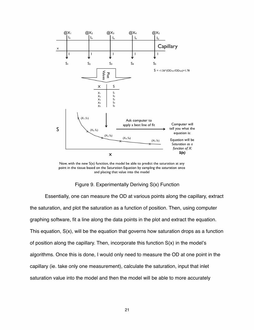
Figure 9. Experimentally Deriving S(x) Function
! Essentially, one can measure the OD at various points along the capillary, extract
the saturation, and plot the saturation as a function of position. Then, using computer
graphing software, fit a line along the data points in the plot and extract the equation.
This equation, S(x), will be the equation that governs how saturation drops as a function
of position along the capillary. Then, incorporate this function S(x) in the modelʼs
algorithms. Once this is done, I would only need to measure the OD at one point in the
capillary (ie. take only one measurement), calculate the saturation, input that inlet
saturation value into the model and then the model will be able to more accurately
21
estimate the saturation at any point in that capillary just from one experimental
measurement.
7 - Conclusion! In sum, the contour plots show accurate estimates of the saturation levels
indicating that the model is performing appropriately. It was also demonstrated that the
model can be used to predict an appropriate selection of finite sensitivity depending on
what hematocrit levels will be dealt with. Resolution was also shown to not have a
significant effect on estimated saturation unless the resolution is decreased by half of
the initial resolution I used. I have also elaborated on an important future idea on how to
improve the practicality of the model by determining a way to derive the true decrease in
saturation function. There are many other areas of the model that can be improved for
future revisions but, as of now, I believe that a solid foundation to a useful and realistic
model with lots of future potential for applications has been laid out by initializing this
project. Some of those next steps toward future improvements would include the
inclusion of complex geometry and multiple capillary networks (which my colleague
Eugene Joh investigated himself in his 6 week project) and hopefully, the successful
modeling of devastating diseases to better our understanding on how to cure them once
and for all.
22

8 - References
1. Professor Dwayne Jackson - MBP 3501 Lecture Notes “Biophysics of Transport
Systems”
2. Dominguez de Villota ED, Ruiz Carmona MT, Rubio JJ, de Andrés S (December
1981). "Equality of the in vivo and in vitro oxygen-binding capacity of haemoglobin in
patients with severe respiratory disease". Br J Anaesth 53 (12): 1325–8. doi:10.1093/
bja/53.12.1325. ISSN 0007-0912. PMID 7317251
3. Mary L Ellsworth, Roland N. Pittman & Christopher G Ellis,“Measurement of
hemoglobin oxygen saturation in capillaries”, 0363-6135/87 1.50 Copyright 1987 the
American Physiological Society
4. Daniel Goldman, Ryon M. Bateman, and Christopher G. Ellis,“Effect of sepsis on
skeletal muscle oxygen consumption and tissue oxygenation: interpreting capillary
oxygen transport data using a mathematical model”,Am J Physiol Heart Circ Physiol
287: H2535–H2544, 2004.
23