South Dakota State University South Dakota State University

Open PRAIRIE: Open Public Research Access Institutional Open PRAIRIE: Open Public Research Access Institutional

Repository and Information Exchange Repository and Information Exchange

Electronic Theses and Dissertations

2018

Modeling Soil Organic Carbon in Select Soils of Southeastern Modeling Soil Organic Carbon in Select Soils of Southeastern

South Dakota South Dakota

Shaina Westhoff South Dakota State University

Follow this and additional works at: https://openprairie.sdstate.edu/etd

Part of the Plant Sciences Commons, and the Soil Science Commons

Recommended Citation Recommended Citation Westhoff, Shaina, "Modeling Soil Organic Carbon in Select Soils of Southeastern South Dakota" (2018). Electronic Theses and Dissertations. 2656. https://openprairie.sdstate.edu/etd/2656

This Thesis - Open Access is brought to you for free and open access by Open PRAIRIE: Open Public Research Access Institutional Repository and Information Exchange. It has been accepted for inclusion in Electronic Theses and Dissertations by an authorized administrator of Open PRAIRIE: Open Public Research Access Institutional Repository and Information Exchange. For more information, please contact michael.biondo@sdstate.edu.

MODELING SOIL ORGANIC CARBON IN

SELECT SOILS OF SOUTHEASTERN SOUTH DAKOTA

BY

SHAINA WESTHOFF

A thesis submitted in partial fulfillment of the requirements for the

Master of Science

Major in Plant Science

South Dakota State University

2018

iii

This thesis is dedicated to my son, Little Paul.

I hope you are always curious, kind, and nurture a good sense of humor. So far, so good.

iv

ACKNOWLEDGEMENTS

I would like to thank the Department of Agronomy, Horticulture, and Plant

Science for funding my project and for being composed of generous individuals who

helped me complete my thesis. Many, many thanks to my advisor, Dr. Douglas Malo, for

his guidance, support, thoughtfulness, and continuously calm demeanor. Mary Malo was

a welcome pillar of support for me (and for Little Paul) throughout my graduate

education. My committee members, Dr. Sandeep Kumar, Dr. Cheryl Reese, Dr. Peter

Sexton, and Dr. Yi Liu, have been invaluable to my thesis research. Thank you. I would

also like to thank Christine Morris of the SDSU Soil Testing Lab for offering me multiple

protocols and hands-on training in the lab. Muhammed Koparan was the best friend and

peer I could have asked for. Hours were spent in the field in a variety of conditions

without a single complaint or opt to quit early…except that one time with the horses.

Little Paul loved spending his days with Nur while we were sampling. I am excited to

come visit you all in Turkey someday. Also, many thanks to Dr. Gary Hatfield with the

South Dakota State University Mathematics and Statistics Department for the numerous

hours spent assisting me with data analysis. That process would have been very painful

without your expertise. Additionally, Mr. Ahmed El-Magrous in the SDSU Mathematics

and Statistics Department was a valuable resource for me concerning the processes

involved in website and mobile application construction.

Thank you to Mr. Anthony Bly and Mrs. Sara (Berg) Bauder for helping me

locate producers to work with for this research. Thank you to Mr. Amundson, Mr.

Blindert, Mr. Fahlberg, Mr. Hanson, Mr. Huls, Mr. Jensen, Mr. Miron, Mr. Nelson, Mr.

Oyen, Mr. Stiefvater, Mr. VanHeerde, and Mr. Westhoff for participating in this project.

v

Thank you to Mr. Pete Bauman and Mr. Benjamin Carlson of the SDSU Extension

Service for teaching me how to use their “Quantifying Undisturbed (Native) Lands in

Eastern South Dakota: 2013” data in Google Earth.

Finally, thank you to my family. To my mom and dad who encouraged me to

continue my education and who offered much support throughout my studies. To my

siblings and siblings-in-law who always had an open ear and sound advice. To my

husband who made numerous sacrifices such that I could leave a well-paying job, health

insurance, and a company vehicle to pursue my degree. You are the epitome of a

supportive spouse; thank you.

vi

TABLE OF CONTENTS

LIST OF TABLES…………………………………………………………………. xv

LIST OF FIGURES………………………………………………………………… xvi

ABSTRACT………………………………………………………………………… xvii

CHAPTER 1: INTRODUCTION & LITERATURE REVIEW…………………… 1

Introduction………………………………………………………………….. 1

Global Carbon Cycle………………………………………………………… 3

Soil Organic Carbon…………………………………………………………. 4

Losses of SOC………………………………………………………… 4

Additions to SOC……………………………………………………… 6

Factors that Impact SOC……………………………………………………... 6

Temperature and Moisture……………………………………………. 7

Texture, Soil Taxonomy, Topography………………….……………... 11

Soil Organisms………………………………………………………… 16

Vegetative and Residue Cover………………………………………… 18

Rotation and Cropping Intensity……………………………………… 23

Fertilizer Amendments………………………………………………… 27

Tillage…………………………………………………………………. 32

Building SOC in the Agricultural Landscape………………………………... 37

Current Carbon Models………………………………………………………. 38

Conclusion...………………………………………………………………….. 41

vii

Literature Cited...…………………………………………………………….. 43

CHAPTER 2: MATERIALS AND METHODS…………………………………… 49

Introduction and Objectives…...……………………………………………... 49

Location Descriptions………………………………………………………... 49

Experimental Design..………………………………………………………... 57

Sample Collection…..………………………………………………………... 57

Laboratory Analysis..………………………………………………………... 58

Electrical Conductivity and pH………………………………………. 58

Soil Organic Matter……………………………………………………. 59

Soil Inorganic Carbon…………………………………………………. 60

Total Carbon and Total Nitrogen…………………………………...…. 61

Water Stable Aggregates………………………………………………. 61

Particle Size……………………………………………………………. 63

Soil Color………...……………………………………………………. 66

Statistical Analysis..……………………………………………...…………... 67

Literature Cited...…………………………………………………………….. 69

CHAPTER 3: RESULTS AND DISCUSSION..…………………………………… 71

Descriptive Statistics………………….….…………………………………... 71

Effect of Depth and Treatment on Soil Properties……….……………. 71

Model Construction....………………………………………………………... 80

Multiple Linear Regression, Stepwise Selection, and Filtered Models 80

viii

Electronic Application Development….……………………………………... 84

Literature Cited...…………………………………………………………….. 87

CHAPTER 4: CONCLUSION..……..……………………………………………… 88

APENDIX A……………………………………………………………………....... 90

APPENDIX B………………………………………………………………………. 106

ix

ABBREVIATIONS

α Alpha: Pertains to the Confidence Interval Set for the Study

°C Degrees Centigrade

δC Change in Carbon

µg Microgram (0.001mg)

µm Micrometer (0.001mm)

1-L One-Liter

1:1 clay One Tetrahedral Layer to One Octahedral Layer per Clay Mineral (e.g. kaolinite)

2:1 clay Two Tetrahedral Layers to One Octahedral Layers per Clay Mineral (e.g. smectite)

AB Five-Year Rotation with One Year of Hay or Root Crop

AeroGRID European Satellite Imagery Database

AF Five-Year Rotation with Two Years of Fallow

ANOVA Analysis of Variance

BBS Back Backslope

BCE Before the Common Era

BF Base Factor

BFS Back Footslope

BMP's Best Management Practices

BS Backslope

C Carbon

C:N Carbon to Nitrogen Ratio

12C Natural Carbon

13C Radioactive Carbon Isotope

13C‰ Parts per Thousand of Radioactive Carbon

CA California

x

CEC Cation Exchange Capacity

CENTURY Plant-Soil Nutrient Cycling Model Produced by Colorado State Univeristy

CF Chinese Fir Plantation

cm Centimeter

CO2 Carbon Dioxide

COMET-Farm Carbon Footprint Model for Industrial Operations

CON Continuous Corn

cPOM Coarse Particulate Organic Matter

CRP Conservation Reserve Program

CT Conventional Tillage

DayCENT Submodel of the CENTURY Model which Operates on a Daily Timescale

DI Deionized

DIC Dissolved Inorganic Carbon

DNA Deoxyribonucleic Acid

DOC Dissolved Organic Carbon

DRFIT Diffuse Reflectance Infrared Fourier Transform spectroscopy

EC Electrical Conductivity

ESRI Environmental Systems Research Institute- Satellite Imagery Software Developers

e.g. For Example

et. al. And Others

FAME Fatty Acid Methyl Ester

FL Farm Land

FLF Free Light Fraction

fPOM Fine Particulate Organic Matter

FS Footslope

FYM Farm-Yard Manure

xi

g Gram

GEOeye Supplier of Satellite Imagery

GIS Geographic Information System

H Climate Region

H, h Land Use and Management Identification

ha, ha-1 Hectare, Per Hectare

HCl Hydrochloric Acid

HF Minimal Associated Heavy Fraction

HT Heated Weight

i.e In OtherWords

IC Inorganic Carbon

IF Input Factor

IG Ignition Weight

IGN French National Geographic Institute

IPCC Intergovernmental Panel on Climate Change

K Potassium

kg, kg-1 Kilogram, Per Kilogram

km Kilometer

LA Land Area

LBS Lower Backslope

LC3 Three-Year Grass-Clover Rotation

LC8 Eight-Year Grass-Clover Rotation

Ley Perennial Crop

LFOC Light Fraction Organic Carbon

LN3 Three-Year Grass with Nitrogen Fertilizer

LN8 Eight-Year Grass with Nitrogen Fertilizer

xii

LOC Labile Soil Carbon

LSD Least Significant Difference

Lu Alfalfa

m, m2 Meter, Square Meter

MBC Microbial Biomass Carbon

Mg Megagram

MID Mid-Intensity Rotation

MinOM Mineral Organic Matter

mL Milliliter

mm Millimeter

MLR Multiple Linear Regression

MLRA Major Land Resource Area

mm Millimeter

MNDA Minnesota Department of Agriculture

MWD Mean Weight Diameter

N Normality

°N Degrees North

N, 14N Nitrogen

15N Radioactive Nitrogen Isotope

NF Native Forest

NO3-1-N Nitrate Nitrogen

NPK Nitrogen, Phosphorus, Potassium

NPP Net Primary Production

NRCS Natural Resources Conservation Service

NT No-Till

NTVG Native Grass, Native Vegetation

xiii

NW Native Woodlots

OH Ohio, USA

OLF Occluded Light Fraction

OM Organic Matter

p p-value: Probability-value

P Phosphorus

PET Potential Evapotranspiration

PFLA Phospholipid Fatty Acid

Pg Petagram

pH Soil Acidity

PM P. massoniana plantaion

POC Particulate Organic Carbon

POM Particulate Organic Matter

ppm Parts Per Million

Q10 Soil Organic Matter Reaction to Temperature

QIIME Quantitative Insights into Microbial Ecology

r2 Coefficient of Determination

R2 Multiple Correlation Coefficient

RC Reference Carbon Stock

RCP(2.6; 8.5) Representative Concentration Pathway

RDF Recommended Dose of Fertilizer

RothC Carbon Cycling Model Created by Rothamsted Research, United Kingdom

RP Robinia pseudoacacia L.

RSE Reference Surface Elevation fo Soil

S Sulfur

SCS Soil Conservation Service

xiv

SEM Structural Equation Modeling

SH Shoulder Hillslope Position

SHB Shoulder Backslope

SIC Soil Inorganic Carbon

SM Summit

SOC Soil Organic Carbon

SOM Soil Organic Matter

SPADE2 Soil Profile Analytical Database for Europe

SYI Sustainable Yield Index

t, t a-1, t ha-1 Ton, Ton per Acre, Ton per Hectare

TC Total Carbon

TC:TN Total Carbon to Total Nitrogen Ratio

TF Tillage Factor

TK Total Potassium

TN Total Nitrogen

TOC Total Organic Carbon

TP Total Phosphorus

TS Toeslope

UBS Upper Backslope

USA United States of America

USDA United States Department of Agriculture

USGS United States Geological Survey

°W Degrees West

WF Wheat-Fallow Rotation

yr, yr-1 Year, Per Year

xv

LIST OF TABLES

Table 2.1: Soil sample general location, map unit, soil composition, and

classification of the soils included in study…………………………………..……… 55

Supplemental Table A1: Specific management information for study sites………... 91

Supplemental Table A2: Sample mean, standard deviation (σ), and Coefficient of

Variation (C.V.) values between replicates for sand content (%), clay content (%),

electrical conductivity (EC, µS/cm), and soil pH by depth. Small letters following

mean values indicate significant differences at α=0.05. …...……………………….. 94

Supplemental Table A3: Sample mean, standard deviation (σ), and Coefficient of

Variation (C.V.) values between replicates for soil organic carbon (SOC, %), soil

inorganic carbon (SIC, %), total carbon (TC, %), and total nitrogen (TN, ppm) by

depth. Small letters following mean values indicate significant differences at

α=0.05.……………………………………………………………………………….. 97

Supplemental Table A4: Sample mean, standard deviation (σ), and Coefficient of

Variation (C.V.) values between replicates for sand content (%), clay content (%),

electrical conductivity (EC, µS/cm), and soil pH by treatment. Small letters

following mean values indicate significant differences at α=0.05.………………….. 100

Supplemental Table A5: Sample mean, standard deviation (σ), and Coefficient of

Variation (C.V.) values between replicates for soil organic carbon (SOC, %), soil

inorganic carbon (SIC, %), total carbon (TC, %), and total nitrogen (TN, ppm) by

treatment. Small letters following mean values indicate significant differences at

α=0.05……………………………………………………………….……………….. 103

Supplemental Table B1: Example of results for stepwise selection in R 3.5.0. This

data refers to the initial reduced model expressed in Equation 3.3. Model 8 was the

model selected for the reduced model due to a high Adjusted R2 and low AIC

value……………………………………………………………...…..…………….... 115

Supplemental Table B2: Model Index 8 was the model selected for the reduced

model expressed in Equation 3.3 based on information in Table B2 due to a high

Adjusted R2 and low AIC value.…………………………………………………… 116

xvi

LIST OF FIGURES

Figure 2.1: MLRA Information and sample locations……………………………… 51

Figure 2.2: Illustration of design used for replicate collection……………………... 58

Figure 3.1: Effect of depth and treatment on soil pH………………………...……... 75

Figure 3.2: Effect of depth and treatment on Electrical Conductivity……………… 76

Figure 3.3: Effect of depth and treatment on Total Nitrogen……………………….. 77

Figure 3.4: Effect of depth and treatment on Total Carbon………………………… 78

Figure 3.5: Effect of depth and treatment on Soil Organic Carbon………………… 79

Figure 3.6: Visual representation pertaining to the steps involved in electronic

application development and their components…………………………………….. 86

Supplemental Figure B1: Boxplot illustrating the distribution of SOC data by

different tillage practices…………………………………………………………… 107

Supplemental Figure B2: Boxplot illustrating the distribution of SOC data by crop

rotation………………………………………………………………………………. 108

Supplemental Figure B3: Boxplot illustrating the distribution of SOC data by

different periods of time under No-Till management………………………………. 109

Supplemental Figure B4: Boxplot illustrating the distribution of SOC data by

Sample Location…………………………………………………………………… 110

Supplemental Figure B5: Plotted residuals for the full model expressed in Equation

3.1. Plot generated in R 3.5.0………………………………………………...……... 111

Supplemental Figure B6: Plotted residuals for the reduced model expressed in

Equation 3.3. Plot generated in R 3.5.0…………………………………..…………. 112

Supplemental Figure B7: Plotted residuals for the final reduced model expressed in

Equation 3.4 after Tillage had been removed. Plot generated in R 3.5.0………….... 113

Supplemental Figure B8: Plotted residuals for the filtered model expressed in

Equation 3.5………………………………………………………………………..... 114

xvii

ABSTRACT

MODELING SOIL ORGANIC CARBON IN

SELECT SOILS OF SOUTHEASTERN SOUTH DAKOTA

2018

Soil organic matter (SOM) is composed of living biomass, dead plant and animal

residues, and humus. Humus is a class of complex, organic molecules that are largely

responsible for improving soil water holding capacity, nutrient mineralization, nutrient

storage, and other critical soil functions. Soil organic carbon (SOC) accounts for

approximately 60 percent of SOM and thus SOC is recognized as a strong indicator of

soil health. Land use changes and intense cultivation of arable soils in the United States

over the past century have led to large decreases in SOM.

The objective of this research was to develop a multiple linear regression model

to predict SOC levels in select southeastern South Dakota soils and the region.

Conventional Till (CT), No-Till (NT), and Native Grass (NTVG) management systems

were studied within South Dakota Major Land Resource Area 102B, 102C, and McCook

County, South Dakota. It was hypothesized that NTVG treatments would have the

highest SOC levels, followed by NT treatments, and CT treatments would have the least.

Samples were analyzed for pH, electrical conductivity (EC), total nitrogen (TN), total

carbon (TC), SOM, soil inorganic carbon (SIC), particle size, color, and water stable

aggregates.

Management was found to have a significant effect on soil pH, EC, TN, TC, and

SOC compared to native conditions (p<0.05). Multiple linear regression (MLR) was used

SHAINA WESTHOFF

xviii

to build the full SOC prediction model which was then reduced using stepwise selection

in R 3.5.0. The final reduced model that was produced by stepwise selection is defined as

SOC = 3.25 - 0.811(Conventional Tillage) - 0.939(No-Tillage) - 0.548(10-20 Depth) -

0.918(20-40cm Depth) + 0.0396(Moisture) - 0.288(Temperature). Although this model

did not result in an acceptable Shapiro-Wilk p-value, the model did not have

multicollinearity issues, and approximately 67% of the variation in SOC was explained

by the model.

To create a model that includes all management variables, filtering the data set to

include only specific data points before running MLR analysis is an option. One proposed

filtered model incorporates No-Till management and Corn-Soybean rotation data points.

The resulting filtered model is defined as SOC = -0.0885 - 0.473(10-20cm Depth) -

0.082(20-40cm Depth) + 0.067(Moisture) - 0.267(Temperature) + 0.156(pH). This model

produced an acceptable Shapiro-Wilk p-value (p=0.969), displayed approximately normal

residuals, and did not exhibit multicollinearity. Approximately 64% of the variation in

SOC was explained by the model. Based upon these results, filtering the data set is an

appropriate method for data analysis and model construction. Developing an electronic

application for use via website or mobile device as a means of sharing this information

with producers is a viable option.

Additional data is needed to improve the models, to meet the assumptions of

multiple linear regression when using stepwise selection, and to increase the applicability

of the model to producers in southeastern South Dakota and the region before the

electronic application is constructed. Furthermore, more data points are needed to

validate the proposed models.

1

CHAPTER 1: INTRODUCTION AND LITERATURE REVIEW

Introduction:

Soil is a complex medium that is responsible for the anchoring of plants, storage

of water and nutrients, support of soil microbial life, and many other tasks that are

essential to crop production (Brady and Weil, 2017). The health of the soil is critical to

successful and sustainable crop production. Soil health is, “the capacity of soil to function

as a vital living system, within ecosystem and land-use boundaries, to sustain plant and

animal productivity, maintain or enhance water and air quality, and promote plant and

animal health” (Doran and Zeiss, 2000). Physical and chemical properties, such as bulk

density, aggregate stability, electrical conductivity (EC), soil organic matter (SOM), and

soil organic carbon (SOC) serve as indicators of soil health (NRCS, 2015). Soil organic

matter is a fundamental component of the soil matrix in terms of water holding capacity,

cation exchange capacity (CEC), nutrient storage, microbial health and other primary soil

functions (Brady and Weil, 2017). Aside from living biomass and decaying plant and

animal tissues (Fenton, et.al, 2008), SOM is composed of humus; a complex, organic

molecule that is largely responsible for the critical soil functions mentioned above

(deHaan, 1977). Nearly 60 percent of humus is composed of SOC and is a strong

indicator of soil health (Soil Survey Staff, 1999).

A brief tour through human history solidifies the importance of soil health to the

security of human civilization. Salinization of arable ground from salt-laden irrigation

water reduced Sumerian harvests to one third of original production between 3000 Before

the Common Era (B.C.E.). and 1800 B.C.E. (Montgomery, 2007). Plato of Ancient

2

Greece wrote, “The rich, soft soil has all run away leaving the land nothing but skin and

bone” concerning the effect of erosion on Greece’s soil (Montgomery, 2007). Man-

induced erosion has worn the Jordan Valley, a once fertile agricultural center in the

Middle East, down to bedrock (Lowdermilk, 1948). The Dust Bowl in the American

Great Plains during the late 1800’s through the 1930’s was another historical period of

soil degradation as intensive cultivation of fine-textured soils and removal of perennial

vegetation severely damaged soil quality (Montgomery, 2007). It is estimated that this

period in U.S. history led to a 40-50% reduction in SOM (Clay et. al, 2017). The Dust

Bowl led to the creation of the Soil Conservation Service (SCS) that has since become

the Natural Resources Conservation Service (NRCS) (Helms, 1992). Events like the Dust

Bowl have shaped our nation and serve as powerful reminders of the consequences of

poor land stewardship.

Soil is a finite resource and yet 2.7 tons per acre per year (t a-1 yr-1) of soil are lost

in the United States (Nearing et. al., 2017). Land use change from native prairie to row

crop can result in a 90% reduction in labile SOC within a century of cultivation (Brady

and Weil, 2017). An estimated 20-43% reduction in SOC has been witnessed around the

world as native forest is converted to farm ground (Wei et. al., 2014b). This literature

review will address the role of SOC in the global carbon cycle, abiotic factors and

agricultural management systems that impact SOC levels, and offer a brief synopsis of

the parameters and applications of select current SOC models.

3

Global Carbon Cycle:

Earth’s carbon (C) exists in three primary reservoirs; aquatic ecosystems,

terrestrial ecosystems, and the atmosphere (Post et. al., 1990). Carbon is constantly in

flux between these reservoirs due to additions and losses from the overall carbon system.

Of the primary C reservoirs, oceans serve as the largest sink for C in the form of

dissolved inorganic carbon (DIC), dissolved organic carbon (DOC), and particulate

organic carbon (POC) (Post et. al., 1990). Oceans and lakes store 40,000 petagrams (Pg)

of carbon (Brady and Weil, 2017). Terrestrial ecosystems serve as the second largest C

sink at almost 3,000 Pg of C storage between Earth’s vegetation and soil (Brady and

Weil, 2017). Above ground vegetation is responsible for storing 550 Pg of C yr-1 while

soils store 2,450 Pg C yr-1 (Brady and Weil, 2017). The atmosphere historically holds the

least amount of carbon at 760 Pg of C (Brady and Weil, 2017). Burning of fossil fuels,

land use changes, and increasing human populations around the globe have led to loss of

equilibrium in the C cycle by disproportionately adding carbon dioxide (CO2) to the

atmosphere (Lal et. al., 1998). In 2017, it was estimated that there was 404 parts per

million (ppm) of CO2 in Earth’s atmosphere as compared to the first reading of 315ppm

CO2 at the Mauna Loa Research Facility in Hawaii in 1958 (NOAA, 2017). Restoring

soil organic carbon (SOC) in degraded soils by 0.01% has the potential to sequester the

same amount of CO2 in the soil as is released annually to the atmosphere (Lal et. al.,

1998).

4

Soil Organic Carbon

Soil organic matter can be divided into three fractions; coarse particulate organic

matter (cPOM), fine particulate organic matter (fPOM), and mineral associated organic

matter (MinOM) (Benbi et.al, 2014). Each fraction of SOM is composed of different

materials and represents different pools of C. Coarse POM consists of labile C in the

form of living biomass, plant litter/residues, and organic biomolecules (Clay et. al., 2017;

Benbi et. al., 2014). This pool is subject to change quickly with new additions or losses of

organic materials into the soil (Clark et. al, 2017). Fine fPOM is associated with the slow

C pool, which has a turnover rate of years to decades (Clay et. al., 2017; Benbi et. al.,

2014). Humus is a stabilized material which makes up MinOM, or the recalcitrant C pool,

and is composed of highly decomposed and no longer identifiable tissues as well as

biomolecule conglomerates (Benbi et. al., 2014; Brady and Weil, 2017). Humus is highly

resistant to change over short periods of time and persists in the soil for hundreds to

thousands of years (Clay et. al, 2017). Soil organic matter pools are influenced by

additions and losses of SOC. Biomass removal, erosion, soil respiration, and

mineralization are all modes of C transport from the soil matrix (Rumpel et. al., 2015).

Above and belowground biomass production and organic amendments serve as C

additions to the soil matrix (Curtin, 2012; Rumpel et. al., 2015).

Losses of Soil Organic Carbon:

Predominant losses of SOC include crop removal, erosion, and soil respiration

(Rumpel et. al., 2015). Crop removal directly impacts SOC levels by reducing

aboveground biomass available for C cycling due to the harvesting of grain, silage,

5

and/or stover (Wilhelm et. al., 2004). Erosion is another direct loss of SOC with serious

ramifications in many areas of soil health. In the United States, erosion accounts for the

loss of 1.67 billion tons of soil each year (NRCS, 2015). Soil respiration and SOM

mineralization account for large fluxes of CO2 back to the atmosphere (Brady and Weil,

2017). Soil respiration is the process by which microbial, plant root, and mycorrhizal

organisms decompose organic materials while emitting CO2 (Brady and Weil, 2017).

This decomposition of organic materials leads to the mineralization of inorganic nutrients

from complex organic compounds (Brady and Weil, 2017). Soil respiration is estimated

to attribute 75 Pg C yr-1 back into the atmosphere (Schelsinger and Andrews, 2000). Soil

respiration accounts for a larger flux of C into the atmosphere than net primary

production (NPP) sinks into the soil, because of CO2 production from microbial and root

respiration (Rumpel et. al., 2015; Schelsinger and Andrews, 2000). Various

environmental factors, such as soil temperature, soil moisture, SOC content, and root

density impact the rate of soil respiration (Guo et. al., 2016).

Guo et. al (2016) compared soil respiration rates across three forest treatments;

200-year old native forest (NF), 36-year old Chinese fir (Cunninghamia lanceolata) (CF)

plantation, and 36-year old P. massoniana (PM) plantation. Microbial biomass carbon

(MBC), pH, texture, SOC, nitrogen (N), and phosphorus (P) were measured in the top

0-10 cm. Soil respiration was measured biweekly from October 2010 to September 2012.

Soil organic carbon, total nitrogen (TN), and MBC were significantly higher in the NF

treatment than the CF or PM. The NF treatment additionally had significantly more litter

fall than either plantation treatment. Soil respiration was highly correlated to SOC (R2=

0.918) which led to significantly higher levels of soil respiration in the NF treatment than

6

in the plantation treatments (Guo et. al., 2016). The higher levels of SOC and fine root

biomass in the NF treatment were responsible for increased soil respiration rates (Guo et.

al., 2016). These results indicate that SOC serves as a fuel for soil respiration and for the

release of CO2 from the soil matrix.

Additions to Soil Organic Carbon:

Primarily, plant material (litter) is responsible for the return of organic matter

(OM) to soil and to the formation of SOM (Kogel-Knabner, 2002). Litter composition is

important to microbial decomposition, mineralization, and formation of SOM (Rumpel

et. al, 2015). The carbon to nitrogen ratio (C:N) is a critical component of the

decomposition formula. Infertile, coniferous forest soils have three times the amount of C

on the forest floor as compared to fertile, deciduous forest floors (Buol et. al., 2011).

High C levels in the surface litter cause microbes that are responsible for organic matter

(OM) decomposition to use all available nutrients (nitrogen (N), phosphorus (P), sulfur

(S), etc.) in the soil to complete the decomposition process. This is called the “priming

effect” and can lead to microbial mineralization of stable humus products (Fontaine et.

al., 2011). This impacts the amount of C that can be transferred to SOC (Kirkby et. al.,

2014). Additionally, management of the soil resource has a large impact on additions of

C to the soil.

Factors that Impact Soil Organic Carbon:

A wide range of abiotic and biotic factors affect the amount of SOC that

accumulates in the soil within a given time frame and location. Warm, wet environments

have the potential to sequester more C than dry climates, but are also more susceptible to

7

C losses than more temperate regions (Ogle et. al., 2005). Sandy soils on steep slopes

cannot accumulate the same levels of SOC as finer textured soils in footslope (FS)

positions (Aguilar and Heil, 1988; VandenBygaart, 2016). Microbial activity defines soil

respiration rates and microbial decomposition adds to SOM (Miltner et. al, 2012; Guo et.

al., 2016). Land use change from native conditions to cultivated systems results in

significant decreases in SOM and SOC (Cambardella and Elliott, 1992; Wei et. al.,

2014a). Agriculture has vast impacts on the soil system as a whole, and different

management practices such as residue removal, rotation, fertilizer amendments, and

tillage impact SOC storage (Janzen et. al., 1992).

Temperature and Moisture:

Temperature affects organic matter fractions to different degrees. The impact of

increasing temperature on cPOM, fPOM, and MinOM fractions was measured with

varying organic matter inputs in a rice (Oryza sativa)-wheat (Triticum aestivum) rotation

(Benbi et. al., 2014). Plots either received annual inputs of rice straw and NPK (nitrogen,

phosphorus, potassium) fertilizer, solely NPK fertilizer, farmyard manure, or no organic

inputs. Surface samples were collected from the 0-15cm depth after the wheat crop was

harvested. Samples were sieved to determine the cPOM, fPOM, and MinPOM fractions.

Microbial biomass carbon was measured on non-sieved samples via incubation and

chloroform fumigation extraction. The influence of temperature on mineralization was

assessed for both sieved and un-sieved samples by estimating mineralization coefficients

at 15°C, 25°C, 35°C, and 45°C and using the 𝑄10 function [SOM sensitivity to

temperature (Fang et. al., 2005)] in five different models. Data on mean C stocks and

8

mineralization rates by temperature were subjected to analysis of variance (ANOVA)

(Freund et. al., 2010).

Results showed that cPOM (labile C) composed the smallest portion of whole soil

samples while MinOM (stable C) composed the largest portion. Although cPOM made

up the smallest fraction of organic matter, the most C was mineralized from this fraction

regardless of temperature. At all temperature increments, MinOM appeared to be the least

responsive to temperature changes when compared to cPOM and fPOM. The authors

concluded that while cPOM composes the smallest portion of whole soil, cPOM is

responsible for the largest amount of C mineralization in the soil. Increases in

temperature had a significant effect on cPOM decomposition. Mineral associated organic

matter accounts for the largest portion C in the soil system, but is the least susceptible to

decomposition. Temperature increases did not have a significant effect on MinOM

decomposition. Results such as this indicate that temperature plays a critical role in

decomposition of the labile C pool, but the stabilized C pool is relatively resilient to

temperature increases (Benbi et. al., 2014).

Climate is an important factor in SOC dynamics. The effect of various land

management scenarios on SOC in different climate zones was studied via meta-analysis

of existing data (Ogle et. al., 2005). Researchers hypothesized that long-term cultivation,

tillage, cropping intensity, residue production, organic amendments, and set-aside land

(such as the NRCS Conservation Reserve Program (CRP)) would all have significant

impacts on SOC in tropical and temperate climates with moist and dry moisture regimes.

The Intergovernmental Panel on Climate Change (IPCC) method (Equations 1.1 and 1.2)

was used on 126 data sets pertaining to the above parameters to analyze changes in SOC

9

levels over a minimum 20-year time frame. The change in C (δC) as defined by the IPCC

model is the sum of SOC in last year of the data set (SOC1(h)) minus the SOC in the first

year of the data set (SOC1−20(h)) by climate region (H). SOC(h) is calculated by

multiplying the Reference Carbon Stock (RC), Base Factor (BF), Tillage Factor (TF),

Input Factor (IF), and Land Area (LA) (see Equation 1.2). Reference carbon stocks

represent carbon stocks under native conditions, BF values estimate the change in SOC

from native after long-term cultivation, TF values estimate the effect of tillage on SOC

stocks, IF values estimate the effect of cropping intensity/input levels on SOC stock, and

Land Area (LA) represents the area for a particular land use and management (h).

𝐸𝑞 1.1: 𝛿𝐶 = ∑ (𝑆𝑂𝐶1(ℎ) − 𝑆𝑂𝐶1−20(ℎ))𝐻ℎ=1 (IPCC, 1997)

𝐸𝑞 1.2: 𝑆𝑂𝐶(ℎ) = 𝑅𝐶 ∗ 𝐵𝐹 ∗ 𝑇𝐹 ∗ 𝐼𝐹 ∗ 𝐿𝐴 (IPCC, 1997)

The data sets were divided by climate region and moisture regime in which

Tropical sites were defined as areas with mean annual temperature greater than 20°C

(Ogle et. al., 2005). Sites were defined as Temperate if the mean annual temperature was

less than 20°C (Ogle et. al., 2005). Moist Tropical sites were defined as locations where

the mean annual rainfall was greater than 1000mm and Dry were locations where mean

annual rainfall was less than 1000mm (Ogle et. al., 2005). To define Moist and Dry

temperate sites, the precipitation to potential evapotranspiration (PET) ratio (P:PET) was

used. Ratios greater than one were defined as Moist and ratios less than one were defined

as Dry (Ogle et. al., 2005). Linear mixed-effect models were implemented to incorporate

fixed and random effects into the response variable. The response variable was the ratio

10

of SOC per management parameter to SOC level in native conditions (BF) (Ogle et. al.,

2005). All data sets were limited to the top 30cm soil depth.

From the 126 data sets gathered, 80 pertained to tillage, 31 pertained to rotation

and cropping intensity, 30 pertained to long-term cultivation, and 17 pertained to land

restoration. The largest changes in SOC were seen in Tropical, Moist regions and the

smallest changes were seen in Temperate, Dry regions. Long-term cultivation caused the

largest decrease in Tropical, Moist locations with 58% ± 12% retention in SOC compared

to native conditions (Ogle et. al., 2005). The Temperate, Dry locations were found to

have 82% ± 4% retention compared to native conditions (Ogle et. al., 2005). These

results indicate that only 58% of the native SOC was still present under long-term

cultivation management in Tropical, Moist climates whereas Temperate, Dry climates

retained 82% of the native SOC (Ogle et. al., 2005). Implementing no-till from

conventional tillage resulted in a positive increase in SOC by a factor of 1.10 ± 0.03

(equal to a 10% increase in SOC) in Temperate, Dry regions and a factor of 1.23 ± 0.05

in Tropical, Moist regions (Ogle et. al., 2005). Increasing the cropping intensity by using

higher yielding varieties and/or cover crops led to an increase in SOC with a factor of

1.07 ± 0.05 in dry climates and 1.11 ± 0.05 in moist climates (Ogle et. al., 2005).

Additions of organic amendments in high intensity systems led to an increase in SOC

with a factor of 1.34 ± 0.08 in dry climates and 1.38 ± 0.06 in moist climates.

The data suggests that temperature and moisture play a large role in the reduction

or accumulation of SOC across multiple management practices. Tropical, moist regions

in this study appeared to decline in SOC levels more rapidly with long-term cultivation

than did Temperate, Dry regions (Ogle, et. al, 2005). The authors conclude that, while

11

Tropical, Moist climates accumulate more SOC, they are also more susceptible to SOM

decomposition than Temperate, Dry regions due to changes in management (Ogle et. al.,

2005).

Texture, Soil Taxonomy, and Topography:

Texture, soil classification, and topographic location are related to SOC levels in

the soil landscape. Coarse and fine textured soils affect SOC in different ways. Chemical

protection is the chemical binding of SOM to silt and clay particles (Six et. al., 2002).

Soil clay content influences C concentration of a soil as the structure of clay is composed

of negatively charged binding sites which provide protection for SOM (VandenBygaart,

2016). Texture is the limiting factor for C accumulation in fine-textured soils (e.g.: clay,

silty clay, sandy clay, etc.) whereas organic inputs are the limiting factor for C

accumulation in coarse-textured soils (e.g.: sand, loamy sand, etc.) (Hassink, 1997,

Johnston et. al., 2017).

Six et. al. (2002) analyzed the influence of chemical protection, physical

protection, and biochemical stabilization on SOC content within SOM. Existing surface

soil data (0-10cm) was compiled from cultivated, grassland, and forest ecosystem studies

around the globe. Two soil particle size ranges were analyzed within these studies; clay

(0-20µm) and clay with silt (0-50µm). Regressions between C associated with clay and

silt (g C kg-1 soil) and proportion of silt and clay in the soil (g of silt g-1 of soil and g of

clay g-1 of soil) were performed for all ecosystems and particle sizes. Six et. al. (2002)

found, like Hassink (1997), that all regressions were significant indicating a strong

positive relationship between SOC and silt and clay content. However, Six et al. also

12

found that the y-intercept for the 0-50µm silt and clay size fraction was significantly

higher than the 0-20µm size fraction. Greater levels of C were associated with the 0-

50µm size fraction due to larger aggregates binding together and trapping more C (Six

et.al., 2002). The authors went further to divide the data into 1:1 and 2:1 clays to assess

any potential significance from chemical composition of clay on C content. The data

indicated significantly lower C stabilization in 1:1 clays (e.g. kaolinite) when compared

to 2:1 clays (e.g. smectite). While there are distinct differences in cation exchange

capacity (CEC) and surface area between 1:1 and 2:1 clays, the authors also noted that

most of the 1:1 data was collected in tropical or subtropical regions in which temperature

and moisture would accelerate the decomposition of SOM (Six et. al., 2002). In

summary, Six et. al found that there was a direct link between SOC content and the

combined silt/clay fraction of the soil. They postulated that this information could be

used to determine the point at which soils would be saturated with C and unable to store

more.

VandenBygaart (2016) tested the hypothesis that the C saturation point in a

degraded soil could be calculated by relating clay content to SOC. A total of 433 data sets

from well-drained Ap horizons under numerous management systems, landscape

positions, textures, and soil types in southern Ontario, Canada were analyzed for C

content and clay content (0-20µm). The data set did not include silt information so the

statistical analysis was limited to clay. A third of the data sets used the Walkley-Black

method to measure SOC while the remaining two thirds used dry combustion. To account

for the differences in SOC values, VandenBygaart (2016) multiplied Walkley-Black

values by a conversion factor of 1.25 to equate them to the dry combustion method.

13

Upper boundary analysis was done by dividing clay levels (the independent variable) into

increments of 50g clay kg-1 soil and fitting the maximum values of C (response variable)

within the increments. The upper boundary, or C saturation point, was determined via

regression analysis.

From the available data, VandenBygaart (2016) found that C saturation for soils

with less than 19% clay is approximately 3.5% SOC. In soils with greater than 19% clay,

C saturation is texture dependent. The author acknowledges that although this research

shows 3.5% SOC as the upper boundary for soils with less than 19% clay, management

of sandy and low-clay soils is important for building of SOM and SOC (VandenBygaart,

2016). Organic amendments can add SOM to the soil profile but without the clay and silt

particles to aid in chemical protection, the SOM from organic amendments will be highly

susceptible to decomposition (VandenBygaart, 2016). Additionally, VandenBygaart

(2016) mentions that the potential of high clay soils to hold large amounts of C may not

be realized due to the nature of elevated clay content restricting plant growth and limiting

C inputs.

The world’s soils are amazingly diverse and are products of the region and parent

material from which they were formed. Soil Taxonomy is the system that soil scientists in

the United States use to classify soil relationships as well as the processes that formed

them (Soil Survey Staff, 1999). Work done by Westin and Buntley (1967) illustrate the

diversity of soils within a geographic region, and the effect of taxonomy on soil

properties. Mean annual soil temperature in South Dakota is approximately 8.3°C along

the northern edge of Kingsbury and Brookings Counties. Frigid soil temperature regimes

[mean annual soil temperature is less than 8°C (Soil Survey Staff, 1999)] are located in

14

soils north of this line whereas mesic soil temperature regimes [mean annual soil

temperature is greater than 8°C but less than 15°C (Soil Survey Staff, 1999)] are located

in soils south of this line. Within this study, a 260km transect was laid from Day County

to Clay County in South Dakota. Eight profiles were sampled north of the 8.3°C line on

frigid soils and eight were selected south of the line on mesic soils. All sites were formed

from the same parent material and had been under similar agronomic management. The

profiles were sampled and analyzed for P, N, and C.

Westin and Buntley (1967) determined that in South Dakota soils, there are

significant changes in soil P, N, and C according to soil taxonomy. Moving from north to

south resulted in reductions in aluminum and calcium associated P, whereas iron (Fe) and

reductant P [iron-bound P (Chang and Jackson, 1958)] increased. Both C and N declined

in the A horizon from north to south, but increased in the B horizons. Lower C and N in

the A horizon in southern counties could be due to the increases in temperature and

precipitation leading to higher mineralization rates (Westin and Buntley, 1967). Increases

in C and N in the B horizons was determined to be due to the thicker horizons present in

southern counties as compared to the northern counties (Westin and Buntely, 1967).

Across the soil transect, the changes in soil properties were gradual. However, the

greatest differences were observed at sites that bordered the mean annual soil temperature

line along Kingsbury County and Brookings County where soils changed from frigid

soils in the north to mesic soils in the south (Westin and Buntely, 1967). These results

illustrate the effect of differences in soil classification on soil properties and offer insight

into conclusions that can be drawn from taxonomic information.

15

Topography is another important abiotic factor when assessing SOC dynamics.

Soil solum and horizon structure change with landscape position (e.g. shoulder (SH)

versus toeslope (TS)). An experiment done by Aguilar and Heil (1988) aimed to show the

importance of toposequence and parent material on SOC content. Soils with sandstone,

siltstone, and shale parent materials under pasture and cultivation were located adjacent

to each other in Grant County, ND. The sandstone toposequence was divided into summit

(SM), shoulder (SH), upper backslope (UBS), lower backslope (LBS), footslope (FS),

back backslope (BBS), and back footslope (BFS) landform positions. The siltstone

toposequence was divided into SM, two shoulders (SH & SHB), UBS, LBS, FS, and

toeslope (TS) landform positions. The shale toposequence was divided into SM, SH, BS,

and FS landform positions. Each horizon per toposequence was sampled to a depth of

120cm or to a lithic contact if before 120cm. Bulk density was taken via the core method,

pH was done by saturated paste, SOC was calculated by the Walkley-Black method, TN

assessed via Kjeldahl, and total/organic P were determined by acid extraction and

combustion.

Overall, the sandstone contained the least amount of C for all landscape positions,

followed by siltstone, and shale had the largest amount of C at all landscape positions.

The summit positions statistically had the lowest SOC concentrations whereas the

footslope positions statistically had the greatest. Nitrogen and P followed this trend also.

The authors credited this to greater OM production in footslope positions as well as to

deposition from upper landscape positions (Aguilar and Heil, 1988). This research shows

how location in the toposequence and parent material impact SOC concentrations.

16

Soil Organisms:

Soil is home to billions of living creatures; there are more microorganisms in a

teaspoon of healthy soil than there are people on the planet (Herring, 2010). Soil

microorganisms include diverse species of bacteria, actinomycetes, fungi, nematodes, and

more (Brady and Weil, 2017). Earthworms are important soil macro-organisms that

modify soil structure via ingestion and excretion of soil, effectively mix surface litter

deeper into the soil profile, and impact microbial mineralization (Barre et. al., 2009;

Fahey et. al., 2013). Microbial communities influence the types and quantities of C pools

in the soil (Zhao et. al., 2018). Soil organisms are important to the formation,

accumulation, and mineralization of SOC.

Miltner et. al. (2012) hypothesized that microbial biomass accounts for a

significant portion of particulate SOM. To test this, 13C labeled Escherichia coli (E.coli)

was added to a rye (Secale cereale) cropping system on a Haplic Phaeozem (Typic

Hapludoll) soil. The E.coli accounted for 26% of the naturally occurring MBC in the soil.

Incubation at 20°C lasted up to 224 days depending on treatment. At the end of the

incubation period, it was found that 56% of the 13C labeled MBC had been mineralized

and the remaining 44% was still in the soil. Further analysis of proteins indicated that

75% of the 13C labeled proteins that had been initially added to the soil were converted to

SOM. Given the assumption that 50% of microbial biomass is composed of proteins

(Miltner et. al, 2012), approximately 37.5% of MBC was transferred into SOM. The

authors conclude that roughly 40% of microbial biomass is transformed into SOM

(Miltner et. al, 2012). Research such as this illustrates the importance of healthy

microbial communities on SOC accumulation.

17

As was noted earlier, SOC exists in different pools. Zhao et. al. (2018) studied the

impact of microbial diversity on different SOC pools under afforestation. They monitored

SOC and microbial communities of three Robinia pseudoacacia L. (RP) stands and one

farmland (FL) treatment in Anasi County, China. Tree stands ranged in age from 42

years, 27 years, or 17 years since afforestation. Prior to replanting with RP, the ground

had been farmland. Each treatment was replicated three times, each replicate was divided

into three plots, and each plot was divided into two subplots. Soil samples were collected

from the 0-10cm depth after carefully removing the surface litter layer and analyzed for

bacterial and fungal species composition, MBC, and carbon fractions. Soil organic carbon

was determined via potassium dichromate oxidation, MBC was determined via

fumigation, light fraction organic carbon (LFOC) was determined by sodium iodide

extraction, particulate organic carbon (POC) was determined by sieving, labile soil

carbon (LOC) via potassium permanganate extraction, and DOC via total organic carbon

(TOC) analyzer. Microbial DNA was extracted and quantified by polymerase chain

reaction and using Quantitative Insights into Microbial Ecology (QIIME) software.

Relationships between C fractions, bacterial diversity, abundance, and phyla present in

soil samples was assessed via Spearman’s rank coefficient (Zhao et. al., 2018).

Zhao et. al. (2018) conclude that time, land use, and microbial community have

significant impacts on C pools. Coarse and fine POM, LOC, POC, MBC, and LFOC were

all significantly greater in the 42 year old RP stand when compared to all other

treatments. Robinia pseudoacacia L. (RP) carbon fractions ranged from 27.2% to 94.1%

and were all significantly higher than FL carbon fractions. Bacterial and fungal

diversities were significantly greater in each RP treatment than in the FL treatment. The

18

dominant bacterial phylum in the RP treatments was Proteobacteria, whereas in the FL

treatment Actinobacteria was dominant. Dominant fungal phyla included Ascomycota,

Zygomycota, and Basidiomycota across all treatments but Zygomycota was the largest in

afforested treatments whereas Ascomycota were predominant in FL. Each phylum

consists of many different classes of bacteria or fungi, but specific phyla have a positive

or negative relationship with carbon. Proteobacteria and Zygomyota, the predominant

bacterial and fungal phyla in RP treatments, have a positive correlation with SOC.

Ascomycota, the predominant fungal phylum in the FL treatment, are negatively

correlated to SOC. The authors note that microbial populations are hinged on C and N

inputs into the soil, as dictated by land use, due to the effect those nutrients have on

lignin decomposition. The main highlight of this research is that as microbial diversity

increases in a soil ecosystem, C also increases. Specific bacterial and fungal phyla also

play an important role in C fraction dynamics, and different forms of management dictate

which phyla will be most prevalent in the soil ecosystem (Zhao et. al., 2018).

Vegetative and Residue Cover:

The type of vegetative cover and amount of plant residue covering a soil will

impact SOC accumulation. Conversion of forestland to agricultural ground leads to

significant reductions in SOC (Lemenih et. al., 2005; Wei et. al., 2014a; 2014b).

Similarly, cultivating native prairie soils initiates significant decreases in SOM

(Cambradella and Elliott, 1992; Malo, 2005; Smith, 2008). Removal of crop residues

after harvest is also directly related to decreases in SOM (Wilhelm et. al., 2004; Ruis et.

al., 2018). Aside from directly removing C-laden stover from agricultural fields,

19

secondary impacts of residue removal, such as increased erosion, will compound

reductions in SOC content (Mann et. al., 2002).

Converting native forest to cultivated systems has detrimental impacts on SOC.

Wei et. al. (2014a) studied the effect of vegetation conversion from native forest to

cultivated land on SOC levels. Research was conducted in the Huanglongshan Forest in

Shaanxi Province, China on a Cambisol (Inceptisol). The region is semi-humid with a

temperate climate. Four sample locations were paired by soil type and management

practices. Each location encompassed native forest, 4 year-, 50 year-, and 100 year-long

cultivation treatments within 3km of each other. The native forest was composed of

minimum 200 year-old oak (Quercus liaotungensis Koidz) and birch (Betula platyphylla

Sukaczev) stands with bunge needlegrass (Stipa bungeana Trinius) established on the

forest floor. Cultivated sites had been sown to a millet (Setaria italica L.), maize (Zea

mays L.), and potato (Solanum tuberosum L.) rotation (Wei et. al., 2014a). Bulk density,

SOC, and N samples were collected at 0-10cm and 10-20cm depths. Laboratory analysis

included separating the light and heavy SOM fractions and measuring the natural

abundance of 13C and 15N isotopes.

Wei et. al. (2014a) determined that there were significant decreases in SOM after

conversion from native forest to cropland with the largest decreases witnessed in the 0-

10cm depth. SOC declined by 19% in the first four years of cultivation. Cultivation had

led to a 33% reduction compared to native forest after 50 years of cultivation in the top 0-

10cm depth. In the 10-20cm depth, Wei et. al. (2014a) determined a 3% decrease in SOC

after four years of cultivation and a 16% decrease in SOC after 50 years of cultivation.

Length of cultivation did not significantly impact SOC between 50 and 100 years of

20

cultivation. Additionally, light-fraction OM (LFOM) significantly decreased (34%) after

four years of cultivation in the 0-10cm depth only and was not significantly different

between 50 and 100 years of cultivation. The authors conclude that the most dramatic

losses of SOC occur before 36 years of cultivation on ground converted from native

forest (Wei et. al., 2014).

Cambardella and Elliott (1992) were interested in how changes in cultivation

impact POM in a grassland ecosystem. Native sod, bare-fallow, stubble mulch, and no-till

were all sampled from the 0-20cm depth on a fine-silty, mixed, mesic Pachic Haplustoll

in a temperate climate near Sidney, Nebraska. Mineral-associated and water-soluble C

and N, as well as POM, were separated in the lab. One-way ANOVA was used to

statistically analyze differences between treatments and Fisher’s LSD (Freund et. al.,

2010) was used to test pairwise comparisons.

Results indicated a significantly higher amount of SOC in the native sod than for

any of the tillage treatments. The stubble mulch and no-till treatments exhibited

statistically similar SOC and both had significantly more SOC than the bare-fallow

treatment. Native sod also had significantly higher POM than any of the tillage

treatments. The authors conclude that cultivation leads to reductions in the labile C pool

and reduces overall SOC compared to native conditions (Cambardella and Elliott, 1992).

This research highlights the positive impact of perennial vegetation on SOC stocks.

Crop residues are important sources of C in the soil system. Field residues are

sometimes removed via livestock grazing or are baled for use as animal bedding (Ruis et.

al., 2018) or cellulosic ethanol (Wilhelm et. al., 2007). Significant reductions in C stocks

21

can result from the removal of crop residues. Ruis et. al. (2018) hypothesized that

removal of corn stover as bales or via grazing would significantly reduce C stocks in a

central Great Plains, prairie-derived ecosystem. Ruis et. al. (2018) tested this hypothesis

over a three-year period on a fine-silty, mixed, superactive, mesic, Cumulic Haplustoll

near Gothenberg, Nebraska. Treatments were arranged in a split-strip, split-strip

randomized complete block design. Residue removal treatments were broken into no-

removal, livestock grazing, and stover baling. Each removal treatment took place on one

of two irrigation treatments; full-irrigation and limited-irrigation. Each removal treatment

also took place on two tillage practices; strip-till (20cm deep by 25cm wide tilled in

April) and No-Till. Nitrogen and P fertilizer were applied to all treatments each year. The

University of Nebraska Corn Stalk Grazing Calculator (Stockton and Wilson, 2013) was

used to determine optimal stocking rate for grazing treatments in which the cattle grazed

stalks for five days in the winter. Surface residue was measured using quadrats each

spring and composite soil samples were collected from 0-5cm, 5-10cm, and 10-20cm

depths. The geometric mean diameter of dry and of wet aggregates was analyzed to

assess wind and water erosion potential. Soil organic carbon was measured by

combustion, bulk density was measured by the core method, POM was separated into

cPOM and fPOM via sieving, fatty acid methyl ester (FAME) was used to analyze

microbial community composition, and sorptivity was measured by the single ring

method. Soil organic carbon stocks were calculated using SOC concentration and bulk

density values. For analysis, the fixed effects were residue removal, irrigation level, and

tillage level. The authors tested for correlation at the irrigation and tillage level to avoid

confounding results by unintended interaction.

22

Data indicated that, over the three-year study, baling stalks removed 66% of

residue and grazing removed 24% of residues when compared to the no-removal

treatments. Neither irrigation level nor tillage level had a significant impact on SOC

concentration. However, when analyzing the effect of tillage on SOC stocks, tillage had a

significant impact at the 0-5cm depth (Ruis et. al., 2018). In 2014 there was no significant

difference between grazing and baling treatments, and both had significantly less residue

than the no-removal treatments. However, in 2015 and 2016, baling removed

significantly more residue than the grazing or no-removal treatments, which were

statistically equal. Baling decreased C concentration by 27% in the 0-5cm depth and 12%

in the 10-20cm depth (Ruis et. al., 2018). Baling reduced SOC stocks by 31% over both

tillage systems in the 0-5cm depth when compared to no-removal treatments. Grazing did

not have a significant impact on SOC stocks. No-Till grazing showed 31% greater SOC

stocks than strip-till. Particulate organic matter was significantly decreased in the 0-5cm

depth with residue removal, but no additional interaction between tillage or irrigation was

found. Residue removal reduced cPOM by 82% and fPOM by 27%, whereas grazing

reduced cPOM by 17% and fPOM by 5% when compared to no-removal. These

reductions are likely caused by limited labile C additions to the soil system (Ruis, et. al.,

2018). Additionally, the data indicated that residue removal significantly altered

microbial biomass and community composition, but grazing and no-removal were

generally statistically the same. Baling residue significantly increased wind and water

erosion potential as compared to grazing and no-removal (Ruis et. al., 2018). From this

research, it is evident that crop residues play an important role in C additions to the soil

profile and, inversely, residue removal leads to reductions in SOC.

23

Rotation and Cropping Intensity:

Diverse crop rotations are a means by which producers can spread economic risk

over different commodities, break disease and pest cycles, and improve soil quality

(Zotarelli et. al., 2005; Lakhran et. al., 2017; Manns and Martin, 2017; Jarecki et. al.,

2018). Not all plants have the same potential for building SOC. Some plant species, such

as oats (Avena sativa), will enrich SOC levels in the surface horizon whereas others, such

as tall fescue (Lolium arundinaceum), can enrich SOC down to 60cm (Manns and Martin,

2017). Research has shown that diversifying crop rotations to include legumes and

perennial grasses is an efficient method of increasing SOC even on low OM soils

(Johnston et. al., 2017; Jarecki et. al., 2018).

Although sandy soils are not optimal candidates for building SOC, proper

management and diverse rotations can help maintain current levels and potentially build

SOC levels over time (Johnston et. al., 2017). It was hypothesized that adding perennial

crops (termed “ley crops” within this study) into the crop rotation would build SOC

(Johnston et. al., 2017). This research took place at Rothamsted Farm in Harpenden, UK

on the Woburn ley-crop experiment site, which began in 1938 and is located on a Cambic

Arenosol (Psamment). Ley-crop treatments consisted of either three years safronin

(Onobrychis viciifoilia) or alfalfa (Medicago sativa) (Lu), three years of grass with N

fertilizer (LN3), 8 years of grass with clover (Trifolium spp.) (LC8), or 8 years of grass

with nitrogen fertilizer (LN8). In 1972, safronin and alfalfa were replaced by grass with

clover (LC3). Ley-crop treatments were followed by two years of arable crops which

were tested for yield differences between ley-crop treatments and all-arable crop

treatments. Treatments without a multi-year ley crop in the rotation consisted of a five-

24

year rotation with one year of a hay or root crop (AB) or a five-year rotation in which two

years were bare fallow (AF). Until the 1960’s, farm-yard manure was added every fifth

year to the treatments. Above ground biomass was removed and ley-crops were generally

cut twice a season. Soil samples were collected from 0-23cm and 23-46cm beginning in

1938 and were regularly collected beginning in 1960. Soil was tested for Olsen P,

exchangeable K, exchangeable magnesium (Mg), and pH to ensure nutrients were not

limiting to crop growth. Total carbon (TC) and N were analyzed by combustion. A

conversion factor of 1.72 was used to convert SOC to SOM (Johnston et. al., 2017). SOC

turnover was estimated using the RothC model (Rothamsted Research, 2017).

Initial SOC at this site before starting the rotation study was 0.98% across all

plots. By the early 1960’s, the LN3 treatments exhibited a 1.27% SOC increase compared

to the AB and AF treatments (Johnston et. al, 2017). Safronin or alfalfa (Lu) ley-crops

did not result in an SOC increase. After changing those plots to grass with clover (LC3),

there was a 1.24% increase in SOC which was comparable to the (LN3) treatment

(Johnston et. al, 2017). The AB treatment declined in SOC from 0.98% to 0.91% and the

AF treatment declined from 0.98% to 0.80% (Johnston et. al, 2017). Soil organic carbon

in the LN8 and LC8 rotations increased from 0.98% to 1.42% and 1.40% respectively

(Johnston et. al, 2017). Carbon inputs over the 70-year study period were modeled using

the RothC model. Model predictions for the 70-year period estimated that the AB

treatment had a C input of 140 t/ha, the AF treatment had 122t/ha, LN3 had 189t/ha, and

LC3 had 134t/ha of C input. The model also predicted that most of the C inputs from the

AB factor had been lost due to limited belowground biomass, all C would was lost from

the AF treatment, 96% was lost from the LN3 treatment, and 98% was lost from the LC3

25

treatment (Johnston et. al, 2017). Overall, the RothC model optimistically estimated that

5% of C inputs would be retained in the soil from year to year, but more realistically 3%

or less would remain in this sandy clay loam soil (Johnston et. al, 2017). Although C

retention was low, the authors noted the beneficial impact of ley-crops significantly

increasing SOC over time on a sandy textured soil.

Semi-arid landscapes also are limited in their ability to build SOC. Work done by

Rosenzweig et. al. (2018) in the semi-arid Great Plains suggests, however, that

intensifying the crop rotation can significantly build SOC. Typical crop rotations in the

semi-arid Great Plains include wheat (Triticum aestivum)-fallow system, mid-intensity

rotations, and continuous cropping. Rosenzweig et. al. (2018) hypothesized that

increasing crop rotation intensity would lead to significant increases in SOC, fungal

biomass, and soil aggregation. Research took place in western Nebraska and eastern

Colorado on a variety of soil types. Wheat-fallow (WF), mid-intensity (MID), and

continuous cropping (CON) were the three rotations assessed in this research. Wheat-

fallow rotations are defined as rotations in which winter wheat is raised from September

to July, then the ground is left fallow for 14 months until the next wheat crop is planted.

Mid-Intensity rotations are defined as management systems in which corn (Zea mays),

sorghum (Sorghum bicolor), peas (Pisum sativum), sunflowers (Helianthus annuus), or

another crop well suited to the region is planted in conjunction with wheat. This reduces

the frequency of fallow. Lastly, CON rotations contain no fallow years and a crop was

raised every growing season. Samples were collected on a total of 96 fields that were

under dryland, No-Till management, without manure or compost additions. Of the 96

fields, 54 were located on working farms and the remaining 42 were located at long-term

26

experiment stations. A total of 27 fields were under WF management, 37 were under

MID management, and 26 were under CON management. For comparison purposes only,

six 30 year-old CRP perennial grass plots were also sampled. Potential evapotranspiration

increased along a gradient from 1368 mm per year in Nebraska to 1975 mm per year in

southeastern Colorado.

Samples were collected from 0-10cm and 10-20cm in the fall of 2015 and again in

the spring of 2016. Fall samples were analyzed for SOC, texture, and pH. Spring 2016

samples were analyzed for water-stable aggregates (mean weight diameter), bulk density,

SOC, total nitrogen, and phospholipid fatty acids (PLFA) (Rosenzweig et. al., 2018).

Multiple linear regression and backward selection were used to measure the relationship

between SOC, C concentration, aggregate stability, and microbial PLFA (Rosenzweig et.

al., 2018). Analysis of variance and Tukey Multiple Comparison tests (Freund et. al.,

2010) were used to identify pairwise differences between C and C:N ratios within

different aggregate size classes. This final regression model was tested for fit

(significance) through structural equation modeling (SEM) and improved by adding back

in previously removed covariates until significance was achieved.

Results indicate that SOC increased by 17% in CON rotations over WF at the 0-

10cm depth (Rosenzweig et. al., 2018). There was no difference between CON and MID

treatments. When comparing the whole sample depth (0-20cm), there was a 16% increase

in SOC concentrations for CON treatments over MID treatments. Continuous and MID

treatments reflected approximately 80% and 70%, respectively, of the SOC found in the

30-year old CRP fields. Based on the model, cropping intensity explained roughly 4% of

the SOC variability at both sampling depths, whereas clay content explained

27

approximately 17% of the variability and PET explained approximately 14%

(Rosenzweig et. al., 2018). Mean weight diameter (MWD) of aggregates was twice as

large in CON treatments as in WF treatments after accounting for the role of PET and

clay content on aggregate stability. Mean weight diameter (MWD) of CRP aggregates

were four times larger than CON aggregates and eight times larger than WF aggregates.

Microbial community structure plays a large role in SOC accumulation (Zhao et. al.,

2018). Rosenzweig et. al. (2018) found that microbial communities were significantly

impacted by increasing cropping intensity. Continuous treatments had three times higher

fungi:bacteria ratios compared to WF treatments while MID treatments were not

significantly different from other treatments. Additionally, aggregate stability linearly

increased with fungal biomass and SOC linearly increased with aggregate stability. For

these reasons, increasing cropping intensity directly (greater levels of crop residue

additions) and indirectly (effects on aggregate stability) increases SOC. One more benefit

the authors note concerning increasing cropping intensity is that they did not observe an

increase in N fertilizer application, but did observe an increase in crop production

(Rosenzweig et. al., 2018). This research highlights the importance of vegetative cover on

crop ground and the benefit of increasing the cropping intensity.

Fertilizer Amendments:

Direct and indirect effects on SOC are witnessed with the use of organic and

synthetic fertilizer materials. Organic amendments, such as manure, directly add C to the

soil (Ryals et. al., 2014). Use of organic and/or synthetic fertilizers increases above and

belowground biomass, which indirectly enhances SOC through greater plant additions

(Ryals et. al., 2014). Research in different global regions and under different vegetation

28

has shown that fertilizer amendments build SOC (Srinivasarao et. al., 2012; Ryals et. al.,

2014).

Ryals et. al. (2014) assessed the impact of compost on C and N storage on two

California grassland soils under different biomes over a period of three years. In this

study, the first location focused on valley grasslands at the Sierra Nevada foothills in

Brown Valley, CA on Xerochrept and Haploeralf soils. The second location focused on

coastal grasslands in Nicasio, CA on Haploxeroll and Argixeroll soils. Seasonally, Brown

Valley is hot and dry, whereas Nicasio experiences milder seasons along the coast. Two

treatments were studied at both sites; a one-time compost amendment and a non-amended

control. Compost was analyzed for C and N content, C:N ratio, and particle size classes

before being applied to a thickness of approximately 1.3cm over compost plots. Compost

was applied in December of 2008. Soil samples were collected before compost

application and in mid-summer (corresponding to water years) for three years. Water

years pertain to surface waters and are based on a twelve month period from October 1

through September 30 (United States Geological Survey, 2016). Sample depths in valley

grasslands were 0-10, 10-30, and 30-50cm and sample depths in coastal grasslands were

0-10, 10-30, 30-50, and 50-100cm. Bulk density was collected via the core method.

Carbon and N were analyzed via CN Analyzer, texture was conducted via the hydrometer

method, and pH was measured on a 1:2 soil:water solution. At year three, 0-10cm

samples were collected at all plots and the organic matter was broken into three fractions;

free light fraction (FLF), occluded light fraction (OLF), and mineral-associated heavy

fraction (HF). Occluded light fraction associated C is protected within soil aggregates.

Organic matter decomposition was calculated using ratios derived from Diffuse

29

Reflectance Infrared Fourier Transform spectroscopy (DRFIT) (Ryals et. al., 2014).

Statistical analysis included ANOVA to test for differences in C and N concentrations

and pools for each site. Repeated measures ANOVA analysis was used to identify

interactions between variables.

Soil texture and pH did not vary significantly between the valley and coastal

grasslands, soil bulk density significantly increased with depth at each site, and the

compost amendment had no significant impact on bulk density values at either site. Prior

to compost application, there were no significant differences in C and N concentrations

between treatment plots and C and N significantly declined with depth across all plots. At

the valley site, compost application led to significant increases in C and N concentrations

compared to the control. The increase in C and N were sustained through the three-year

trial. Although C and N increased numerically over the three-year study with compost

application at the valley site, the increase was not significant. At both sites, compost

significantly increased the C content of the FLF organic matter fraction in the 0-10cm

depth. Valley grasslands saw a 26% increase in FLF associated SOC and coastal

grasslands saw a 37% increase in FLF associated SOC over the three year study.

Occluded light fraction organic matter trended upward at both sites but only significantly

increased at the coastal site. Heavy fraction organic matter was unaffected by treatment

and had the lowest C concentration of the three OM fractions, however, it accounted for

most of the C present on a mass basis. Nitrogen concentration was significantly increased

in all OM fractions at the valley site and in the FLF and OLF fractions on the coastal site.

Overall, the C:N ratio decreased with compost addition at both sites. Ryals et. al. (2014)

30

conclude that organic amendments not only increase soil C and N concentrations, but also

protect C and N through the formation of aggregates over a short time period.

Work by Srinivasarao et. al. (2012) assessed the effect of organic and synthetic

fertilizer on SOC sequestration, the relationship of SOC to the sustainable yield index

(SYI), and the amount of C inputs was required to maintain SOC levels. Research took

place on an Udic Ustochrept soil in subhumid, tropical Varanasi, India over a 21-year

period. Seven treatments were studied under rice (Oryza sativa L.)-lentil (Lens esculenta

Moench) rotation in which rice was grown in the rainy season (June-September) and

lentil was grown in the post rainy season (October-December). Treatments were no-

fertilizer control, 100% recommended dose (i.e. recommended application rate) mineral

fertilizer (RDF), 50% RDF, 100% organic Farm-Yard Manure (FYM), 50% RDF with

50% RDF-foliar, 50% FYM with 50% RDF, and Farmer’s Practice of 20kg N ha-1. Each

treatment had three replicates. Farm-Yard Manure was applied at a rate of approximately

10.7 Mg ha-1 and the RDF in the region was a 60-50-30 (N-P-K) blend. All fertilizer was

applied to the rice crop and the legume crop used residual fertility. Three 0.2m long

samples were collected from each plot to a depth of one meter. Samples were analyzed

for pH, carbonates, CEC, texture via hydrometer, and plant available N, P, and K. Bulk

density was collected separately. Above and belowground biomass were measured after

harvest had removed the grain. Carbon stocks were calculated by multiplying SOC

concentration by the soil bulk density, then by the sample depth, and then by a factor of

10. Sequestered C was calculated by the equation: SOCcurrent − SOCinitial. The

sustainable yield index was calculated by subtracting the average crop yield from the

estimated standard deviation, and dividing by maximum yield. The Duncan Multiple

31

Range test (Duncan, 1955) was used to measure differences between means for each

treatment and treatment-wise regression models for rice and lentil were used to determine

the effect of fertilizer on SOC.

Carbon inputs in the control treatment were 1.1 Mg C ha-1 yr-1 whereas the 50%

FYM with 50% RDF treatment had significantly more C input at 2.4 Mg C ha-1 yr-1. All

FYM treatments resulted in an additional 1.77 Mg C ha-1 yr-1 to 3.55 Mg C ha-1 yr-1 when

compared to other treatments. Early in the 21-year study period, yields across mineral

and organic inputs were statistically similar. As the experiment progressed, the 50%

FYM with 50% RDF treatment had the highest yield followed by 100% mineral and

100% FYM. Additionally, treatments with FYM saw better water retention which

improved the SYI values for those treatments. Bulk density was lower in treatments with

FYM when compared to mineral fertilizer or the control treatment. Carbon concentration

in the control treatment declined most significantly in the 0-20cm and 20-40cm depths.

Farm-Yard Manure was able to increase SOC down to 80cm. Overall, SOC stocks were

greatest in the 100% FYM treatment, followed by 50% FYM with 50% RDF, and then

the 100% RDF treatment. The 50% RDF with 50% RDF-foliar treatment had statistically

the same SOC stocks as the 50% RDF and Farmer’s Practice, but significantly more than

the control treatment. In this study, Srinivasarao et. al (2012) calculated that 13.4% of the

C directly applied in the form of FYM was converted into stable SOC stock. Control

treatments saw the largest reduction in SOC stocks (-3.1 Mg C ha-1) and the 100% RDF

treatment did not supply enough C to prevent decreases in SOC stocks (-0.4 Mg C ha-1).

From their calculations, Srinivasarao et. al. (2012) conclude that 2.47 Mg of C ha-1 need

to be added to tropical Inceptisols each year to maintain SOC stocks. Fertilizer

32

amendments can help directly and indirectly add C to the soil to maintain SOC stocks in

agricultural land.

Tillage:

Tillage breaks soil structure and protective aggregates, promotes wind and water

erosion, and accelerates microbial decomposition of labile C (Angers et. al., 1997;

Balesdent et. al., 2000; Mann et. al., 2002; Metay et. al., 2007; Manns and Martin, 2017;

Maillard et. al., 2018). Long-term tillage can lead to substantial reductions in SOC

content compared to SOC under native conditions (Malo et. al., 2005; Franzluebbers and

Stuedemann, 2008). Certain tillage management practices, such as No-Till, have shown

promise in restoring SOC with time (Blanco-Canqui and Lal, 2008; Mishra et. al., 2010;

Engel et. al., 2017).

Prairie-derived soils in the Northern Great Plains are young, fertile soils that are

naturally high in OM and C (Liebig et. al., 2004). Work done by Malo et. al. (2005)

sought to quantify the effect of long-term tillage on various soil properties in the

Northern Great Plains. Research took place on Argiustolls, Natrustolls, Argialbolls,

Calciustolls, Haplustolls, Argiaquolls, Endoaquolls, and Fluvaquents in Beadle,

Minnehaha, McCook, and Union counties in South Dakota. Sample locations coincide

with unpublished data collected between 1919 and 1922 by J.G. Hutton in which Hutton

analyzed TC, SOC, soil inorganic carbon (SIC), TN, total phosphorus (TP), total

potassium (TK), pH, and bulk density on cultivated and uncultivated paired soils. Malo

et. al. (2005) returned to these sample locations 75 years later in 1996 and 1997, and

repeated Hutton’s sample procedure to gather new samples. Some locations that had been

33

uncultivated at the time of Hutton’s work had since been cultivated when Malo et. al.

(2005) returned. In these areas, uncultivated ground on the same soil type was located

within 100m of the original sample site when possible. Based on information from

Hutton’s study, it is known that the cultivated sites had been tilled for greater than 80

years. Sample depths were 0-15, 15-50, and 50-100cm and samples were analyzed for the

same soil properties as Hutton completed in 1922. Bulk density was not collected in

1996/1997 but was estimated based off bulk density values provided by the USDA-

NRCS.

Results from Malo et. al. (2005) indicate significant changes in nitrate nitrogen

(NO3-1-N), extractable P, and extractable K with sample depth and treatment. Nitrate

levels were higher in cultivated treatments compared to uncultivated due to repeated N

fertilizer additions, uncultivated treatments had significantly more P in the 0-10cm depth

than cultivated treatments due to harvest removal in cultivated treatments, and

uncultivated treatments had significantly higher extractable K than cultivated treatments

at all depths due to harvest removal (Malo et. al., 2005). Organic matter is the only

natural source of N in the soil (Brady and Weil, 2017). Total nitrogen significantly

decreased with depth in response to declining humus levels. Additionally, cultivated soils

experienced 20-30% reductions in TN compared to uncultivated; even with fertilizer

additions, high amounts of TN have leached or been harvested. Depth had a significant

impact on TC as well. TC was greatest in the 0-15cm depth for uncultivated soils, but TC

was greatest in the 50-100cm depth for cultivated soils due to carbonate rich parent

material. Effect of parent material on TC is evidenced by SIC measurements in which the

50-100cm depth has significantly greater SIC than either the 0-15 or 15-50cm depths.

34

Cultivated treatments had significantly less SOC than uncultivated at the 0-15 and 15-

50cm depths, but were statistically the same at the 50-100cm depth. A 15-30% reduction

in SOC between cultivated and uncultivated treatments was determined. Changes in bulk

density can have large impacts on a soil’s reference surface elevation (RSE). When bulk

density values increase, soils essentially “sink” from a reduction in pore space. Therefore,

if sampling protocol does not account for changes in RSE corresponding to changes in

bulk density, the potential for incorrect sampling depth increases. Malo et. al. (2005)

corrected the data for these changes in RSE. While the cultivated and uncultivated

treatments had similar TC:TN ratios in the 0-15cm depth, uncultivated treatments had

significantly lower TC:TN ratios at deeper depths than the cultivated treatments. The

TC:TN ratio in uncultivated treatments did not change from 0-15cm to 15-50cm, but that

ratio significantly increased in the 50-100cm depth due to the presence of carbonates. The

TC:TN ratio in cultivated treatments increased with each depth. Decomposition of humus

is evidenced by the SOC:TN ratio, as it significantly decreased in the 0-15cm and 15-

50cm depths for both cultivated and uncultivated treatments. No major changes in

SOC:TN were noted in the 50-100cm depth. Many of the sites were located on landscape

positions that are susceptible to wind and water erosion. Although wind erosion was

minimal due to the soil texture, there was a high risk of water erosion. For this reason,

Malo et. al. (2005) hypothesize that SOC loss in cultivated treatments could in part be

due to soil erosion in this area. Malo et. al. (2005) conclude that C losses from harvest

removal, decomposition of OM, and erosion have caused the greatest losses to SOC in

this study.

35

Cultivation is known to result in lower SOC levels, weaker aggregates, and higher

erosion potential when compared to native systems (Malo et. al., 2005). Work done by

Mishra et. al. (2010) aimed to quantify changes in SOC as land was converted from forest

to crop ground, ascertain the effects of tillage on SOC sequestration, and quantify the rate

of SOC sequestration under different tillage practices in the Corn Belt of Ohio, USA.

Mishra et. al. (2010) hypothesized that reducing soil disturbance with No-Till practices

would lead SOC levels to surpass those of conventional tillage systems. This study was

implemented on three university-conducted long-term tillage experiments and three

producer operated farms in Ohio, USA. The first long-term experiment was located near

Coshocton, OH on a Ultic Hapludult, the second was near South Charleston, OH on a

Aeric Ochraqualf, and the third was near Hoytville, OH on a Mollic Ochraqualf. Producer

locations were near Delaware, OH on an Aquic Hapludalf, near Coshocton, OH on a

Typic Hapludult, and near Hoytville, OH on a Mollic Epiaqualf. A total of three

treatments were studied; native woodlots (NW), chisel plow/conventional tillage (CT)

and no-till (NT). Level of tillage in CT treatments, duration of NT, and crop rotation

varied from location to location. The long-term experiment sites were replicated four

times and the producer-managed sites were analyzed as pseudo-replicates by pairing

samples at each treatment level by soil type and topography.

Soil samples were collected from each treatment in summer of 2006. Bulk

samples and core samples were collected from 0-10cm, 10-20cm, 20-30cm, and 30-40cm

at each treatment. Due to a warm regional climate, organic horizons do not form under

Ohio forests and fresh litter was not included in soil samples of NW or NT treatments

(Mishra et. al., 2010). Samples were analyzed for soil moisture content, bulk density, TC,

36

TN, and isotopic carbon concentration (13C). Relative abundance of 13C was determined

by dividing the ratio of sample 13C and 12C to a reference value. This was subtracted from

1 and multiplied by 1000 to attain 13C ‰. SOC and N pools (stocks) were calculated with

bulk density values and sample depth. One-way ANOVA was used to determine the

effect of tillage on SOC and N concentration, SOC and N stocks, bulk density, and

carbon isotopes at each sample depth (Mishra et. al., 2010).

Bulk density was only mildly impacted by tillage, but was significantly lower in

NW treatment down to 30cm. Native Woodlot bulk density significantly increased in the

30-40cm depth. Tillage had no significant impact on bulk density at the long-term tillage

experiment locations and results were not consistent at the producer locations. At all six

locations, SOC and N levels at the 0-10cm depth were greater in the NW treatment than

in CT or NT treatments. Four of six locations had more SOC and N in the 0-10cm depth

in NT treatments than in CT treatments. There were no significant differences among

SOC and N concentrations at the 10-20cm depth between tillage treatments. Soil organic

carbon and N stocks were significantly greater under NW treatments at all locations.

There was a significant difference between NT and CT for SOC and N stocks at the long-

term experiment locations where NT had been in practice for over 50 years. There was a

lack of SOC and N stock response at the producer locations which the authors note is on

par with similar pseudo-replicate research. Mishra et. al. (2010), postulate that the lack of

response in SOC and N stocks is due to the shorter duration of on-farm NT as compared

to the long-term experiment locations. Based on the overall data from long-term

experiment sites, the authors conclude that converting from CT to NT can lead to a 0.57

Mg ha-1 increase in C annually over the course of 15-20years. From the 13C data, Mishra

37

et. al. (2010) calculated the loss of SOC due to deforestation to range between 26% and

55%. However, by converting management practices from CT to NT, some of that SOC

can be replaced in the soil profile (Mishra et. al., 2010).

Building SOC in the Agricultural Landscape:

Best Management Practices (BMPs) strive to economically, feasibly, and

effectively improve crop production while considering the integrity of surrounding

environmental ecosystems (MNDA, 2017). Best Management Practices can be targeted

toward pest management, erosion management, water quality, soil health, and other

important agronomic issues. Various possible BMPs for increasing SOC accumulation

have already been mentioned in this review such as reducing tillage, increasing cropping

intensity, and maintaining surface residues (Ogle et. al, 2005; Johnston et. al., 2017; Ruis

et. al., 2018). Based on a global review by West and Post (2002), data suggests that

conversion from Conventional Tillage to No-Till can increase C sequestration rates by 57

g C m-2 yr-1. Additionally, increasing rotation intensity can increase C sequestration rates

by 20 g C m-2 yr-1 (West and Post, 2002). The use of cover crops to increase the length of

vegetative cover and increase surface residue within the growing season is another

potential BMP. Another review by Blanco-Canqui et. al. (2015) highlights how the use of

cover crops can increase SOC due to reduced erosion, increased biomass, and improving

other soil properties to facilitate soil aggregation (i.e. limiting soil compaction).

The efficacy of BMPs is hinged on numerous factors. Climate and inherent soil

properties may inhibit SOC accumulation in certain regions. For instance, in research

mentioned earlier in this paper (Johnston et. al., 2017), the cool climate and sandy texture

38

of the soil in the ley crop rotation limited SOC accumulation potential even with diverse

crop rotations. Results of that research concluded that there was still a significant increase

in SOC over time, but a majority of the carbon inputs were not retained in that system.

Time is another restraint on many BMPs in that the positive effects may take many years

to become evident (Mishra et. al., 2010). One study included earlier (Srinivasarao et. al.,

2012), focused on the effect of mineral and organic amendments on SOC. The authors

note that significant differences between mineral and organic amendments on SOC were

minimal until later in the 21-year study period. The benefits of cover crops on SOC are

often not seen in the first few years of implementation (Blanco-Canqui et. al., 2015).

Producers may resist committing to a BMP that will not produce positive results in initial

years of implementation. No-Till is a popular BMP for reducing erosion and improving

soil health, although it is noted that significant changes may only be seen in surface

horizons (West and Post, 2002; Blanco-Canqui and Lal, 2008; Rosenzweig et. al., 2018).

Other problems with BMP implementation exist, such as financial burden of lost

productivity or investment in new equipment, but governmental programs are available to

defray the cost (Dayer et. al., 2018).

Current Carbon Models:

Carbon models have been used in scientific research since the 1940’s and model

development and utilization has been steadily growing with every decade (Campell and

Paustian, 2015). The CENTURY and RothC models account for a majority of SOM

modeling citations and publications (Campbell and Paustian, 2015). The CENTURY

model was developed by the Natural Resource Ecology Laboratory (NREL) at Colorado

State University. Weather data, soil texture, plant nutrient content, lignin content in plant

39

materials, N inputs from the soil and atmosphere, and initial C and N levels are the

necessary inputs for running the CENTURY model which operates on a monthly time

sequence (NREL, 2012). Additional submodels for C, water, grasslands/crop systems,

and forest systems exist to further separate model inputs into more specific groups with

varying turnover rates (NREL, 2012). The CENTURY model has been expanded into the

DayCENT model as well. DayCENT uses similar parameters to CENTURY, but operates

on a daily time sequence (NREL, 2012). The RothC model was developed by

Rothamsted Research in the United Kingdom. Monthly rainfall, monthly evaporation,

monthly mean air temp, clay content, estimated decomposition rate, soil cover, monthly

plant inputs, monthly manure inputs, and soil sample depth are the parameters required

for the RothC model which also operates on a monthly time sequence (Rothamsted

Research, 2017). CENTURY and RothC are complex models that have been utilized for

research experiments focused on long-term impacts of agricultural management or of

climate change on SOC.

Work done by Dintwe and Okin (2018) used the CENTURY model to assess the

impact of anthropogenic climate change on SOC in southern Africa on the Kalahari

savannahs. Four study sites were selected in this region where C, plant biomass, and

nutrient cycling data had been collected in the past. Previously collected soil data,

weather models, and Representative Concentration Pathway (RCP) 2.6 and RCP8.5

[future climate conditions as outlined by the Intergovernmental Panel for Climate Change

(Dintwe and Okin, 2018)] were used to run the CENTURY model. The RCP2.6 scenario

assumes that greenhouse gas emissions peak between the years 2010 and 2020 (IPCC,

2017). The RCP8.5 scenario assumes that emissions will continue to rise throughout the

40

21st century (IPCC, 2017). Simulation began in the year 4000BCE and ended in 2100.

Model results indicate that warming climates are associated with higher concentrations of

CO2 in the atmosphere which will increase plant production. SOC will be negatively

impacted, however, due to large losses of CO2 from microbial respiration that outpace

plant biomass carbon additions to the soil (Dintwe and Okin, 2018).

The RothC model was utilized to assess the effect of compost amendments on

SOC levels in Italitan agricultural soils over a century of use (Mondini et. al., 2012). The

study area encompassed all of Italy, soil data was collected from the Soil Geographical

Database of Europe (Van Liedekerke and Panagos, 2012), bulk density was estimated

through the Soil Profile Analytical Database for Europe (SPADE2) (Hollis et. al., 2006),

a total of 12 different climate scenarios were defined based on data from the IPCC, and

the RothC model was used to simulate changes in SOC from the years 2001 to 2100.

Compost simulations were run on mineral-soils suited for agricultural use; approximately

60% of all soil map units in Italy were included in the compost analysis. The RothC

model predicted a general decline in SOC stocks in association with climate change

scenarios (Mondini et. al., 2012). However, by the addition of compost amendments SOC

stocks could actually increase throughout those same scenarios (Mondini et .al., 2012).

Both the CENTURY and RothC model are well suited for scientific research that

is focused on long-term impacts of management changes or changes in climate. For the

average producer who is interested in potential SOC levels on their operation, however,

the functionality and accessibility of these models is limited. COMET-Farm is a farm-

scale model built by the United State Department of Agriculture that is based on

Colorado State’s DayCENT model (USDA, 2018). COMET-Farm is geared for producers

41

who want to quantify the C footprint of their operation (USDA, 2018). Although this

model is intended for producers, it can be cumbersome and results are not clearly

explained. For this reason, COMET-Farm may be better served for producers to utilize

with the guidance of a local NRCS or Extension Agent to help interpret results.

Contrastingly, models in other disciplines exist that are producer-focused and very easy

to use. One such model is the Fusarium Head Blight Prediction Center model (USWBI,

2008; De Wolf et. al., 2018) which consists of one web-page with three drop down

menus. Producers need only to select their geographic region on the available map, select

their hybrid’s level of resistance to Fusarium head blight, and the length of time in hours

they would like the projection to focus on. Results are concise and clearly illustrated.

Access to a SOC model of similar simplicity would be useful for producers in South

Dakota and the region who are interested in quickly quantifying their operation’s

potential SOC levels.

Conclusion:

Soil is a limited and valuable natural resource. Maintaining soil health for future

generations will be a major challenge as the global population continues to grow and the

demand for food and fiber follow (Lal, 2006). Soil organic carbon is one of three primary

C pools within the global C cycle and maintaining SOC levels can sustain crop

production over time (Post et. al., 1990; Lal, 2006). Numerous factors impact SOC levels

including climate, physical soil properties, soil organisms, plant cover, residue removal,

tillage, and more. Cultivation leads to reduction in SOC due to biomass removal,

destruction of aggregates, erosion, and accelerated microbial respiration (Malo et. al.,

2005; Rumpel et. al., 2015; Brady and Weil, 2017). Certain management practices show

42

promise in returning C to the soil and increasing overall soil health (Assmann et. al.,

2014; NRCS, 2017).

Currently, C models are complex and produce information above and beyond

what is required at a farm-scale for producers in South Dakota and the region. For this

reason, there is a need for a simple and straight-forward SOC prediction model that is

similar in scope to the Fusarium Head Blight Risk Assessment Tool from USWBI.

Construction of this user-friendly model would assist producers in setting relative C level

goals for their operation. With a clear goal in mind, deciding which BMPs to incorporate

into future management decisions will be less intimidating and more useful.

43

Literature Cited:

Angers, D.A., Bolinger, M.A., Carter, M.R., Gregorich, E.G., Drury, C.F., Liang, B.C.,

Voroney, R.P., Simard, R.R. Donald, R.G., Beyaert, R.P., Martel, J. 1997. Impact

of tillage practices on organic carbon and nitrogen storage in cool, humid soils of

eastern Canada. Soil and Tillage Research. 41: 191-201.

Aguilar, R., Heil, R.D. 1988. Soil organic carbon, nitrogen, and phosphorus quantities in

Northern Great Plains rangeland. Soil Science Society of America. 52: 1076-

1081.

Assmann, J.M., Anghinoni, I., Posselt Martins, A., Valadao Gigante de Andrade Costa,

S.E., Cecagno, D., Selau Carlos, F., Cesar de Faccio Carvalho, P. 2014. Soil

carbon and nitrogen stocks and fractions in a long-term integrated crop-livestock

system under no-tillage in southern Brazil. Agriculture, Ecosystems and

Environment. 190: 52-59.

Balesdent, J., Chenu, C., Balabane, M. 2000. Relationship of soil organic matter

dynamics to physical protection and tillage. Soil and Tillage Research. 53: 215-

230.

Barre, P., McKenzie, B.M., Hallett, P.D. 2009. Earthworms bring compacted and loose

soil to a similar mechanical state. Soil Biology and Biochemistry. 41: 656-658.

Benbi, D.K., Boparai, A.K., Brar, K. 2014. Decomposition of particulate organic matter

is more sensitive to temperature than the mineral associated organic matter. Soil

Biology and Biogeochemistry. 70: 183-192.

Blanco-Canqui, H., Lal, R. 2008. No-tillage and soil-profile carbon sequestration: an on-

farm assessment. Soil Science Society of America Journal. 72(3): 693-701.

Blanco-Canqui, H., Shaver, T.M., Lindquist, J.L., Shapiro, C.A., Elmore, R.W., Francis,

C.A., Hergert, G.W. 2015. Cover crops and ecosystem services: Insights from

studies in temperate soils. Agronomy Journal. 107(6): 2449-2474.

Brady, N and Weil, R. 2017. The Nature and Property of Soils. Harlow, England. Pearson

Education Limited.

Buol, S.W., Southard, R.J., Graham, R.C., McDaniel, P.A. 2011. Soil Genesis and

Classification. Chichester, West Sussex: Wiley-Blackwell. ISBN-10:0-8138-

0769-7.

Cambardella, C.A., Elliott, E.T. 1992. Particulate soil organic matter changes across a

grassland cultivation sequence. Soil Science Society of America. 56: 777-783.

Campbell, E. E. and Paustian, K. 2015. Current developments in soil organic matter

modeling and the expansion of model applications: a review. Environmental

Research Letters. 10: 123440.

Chang, S.C., Jackson, M.L. 1958. Soil phosphorus fractions in some representative soils.

European Journal of Soil Science. 9 (1): 109-119.

Clark, K.M., Boardman, D.L., Staples, J.S., Easterby, S., Reinbott, T.M., Kremer, R.J.,

Kitchen, N.R., Veum, K.S. 2017. Crop yield and soil organic carbon in

conventional and no-till organic systems on a claypan soil. Agronomy Journal.

109(2): 588-599.

Clay, D.E., Chang, J., Reicks, G., Clay, S.A., Reese, C. 2017. Calculating soil organic

turnover at different landscape positions in precision conservation. Precision

Conservation: Geospatial techniques for agricultural and natural resources

44

conservation. Agronomy Monograph 59. doi:10.2134/agronmonogr59.2013.0028

Curtin, D., Beare, M.H., Hernandez-Ramirez, G. 2012. Temperature and Moisture Effects

on Microbial Biomass and Soil Organic Matter Mineralization. Soil Science

Society of America Journal. 76:2055-2067.

Dayer, A.A., Lutter, S.H., Sesser, K.A., Hickey, C.M., Gardali, T. 2018. Private

Landowner Conservation Behavior Following Participation in Voluntary

Incentive Programs: Recommendations to Facilitate Behavioral Persistence.

Conservation Letters. doi: 10.111/conl.12394.

de Hann, S. 1997. Humus, its formation, its relation with the mineral part of the soil and

its significance for soil productivity. Organic matter studies. 1, 21-30.

De Wolf, E., Paul, P., Madden, L., Imhoff, K., Person, A., Miller, D., Crawford, S., Auer,

T., Anderson, M., Ketchum, B., Brown, J., Akyuz, A., Carcoana, R., Guinan, P.

Accessed 2018. Fusarium Head Blight Prediction Center.

http://www.wheatscab.psu.edu/

Dintwe, K., Okin, G.S. 2018. Soil organic carbon in savannahs decreases with

anthropogenic climate change. Geoderma. 309: 7-16.

Doran, J.W. and Zeiss, M.R. 2000. Soil Health and Sustainability: Managing the biotic

component of soil quality. Applied Soil Ecology, 15(1): 3-11.

https://doi.org/10.1016/S0929-1393(00)00067-6.

Duncan, D.B. 1995. Multiple range and multiple F tests. Biometrics. 11(1): 1-42.

Engel, R., Miller, P.R., McConkey, B.G., Wallander, R. 2017. Soil organic carbon

changes to increasing cropping intensity and no-till in a semiarid climate. Soil and

Water Management and Conservation. 81(2): 404-413.

Fahey, T.J., Yavitt, J.B., Sherman, R.E., Maerz, J.C., Groffman, P.M., Fisk, M.C.,

Bohlen, P.J. 2013. Earthworm effects on the incorporation of litter C and N into

soil organic matter in a sugar maple forest. Ecological Applications. 23(5): 1185-

1201.

Fang, C., Smith, P., Moncrieff, J.B., Smith, J.U. 2005. Similar response of labile and

resistant soil organic matter pools to changes in temperature. Nature. 433: 57-59.

Fenton, M., Albers, C., Ketterings, Q. 2008. Soil Organic Matter. Cornell University

Cooperative Extension. Fact Sheet 41.

Fontaine, S., Henault, C., Aamor, A., Bdioui, N., Bloor, J.M.G., Maire, V., Mary, B.,

Revaillot, S., Maron, P.A. 2011. Fungi mediate long term sequestration of carbon

and nitrogen in the soil through their priming effect. Soil Biology and

Biochemistry. 43: 86-96.

Franzluebbers, A.J., Stuedemann, J.A. 2008. Early response of soil organic fractions to

tillage and integrated crop-livestock production. Soil Biology and Biochemistry.

72(3): 613-625.

Freund, R.J., Wilson, W.J., Mohr, D.L. 2010. Statistical methods, 3rd Edition. Academic

Press, Burlington, MA.

Guo, J., Yang, Z., Lin, C., Liu, X., Chen, G., Yang, Y. 2016. Conversion of a natural

evergreen broadleaved forest into coniferous plantations in a subtropical area:

effects on composition of soil microbial communities and soil respiration.

Biology and Fertility of Soils. 52: 799-809.

Hassink, J. 1997. The capacity of soils to preserve organic C and N by their association

with clay and silt particles. Plant and Soil. 191(1): 77-87.

45

Helms, D. 1992. Readings from the history of the Soil Conservation Service. USDA

Economics and Social Sciences Division. Historical Notes Number 1.

Herring, P. 2010. The secret life of soil. Oregon State University Extension Service.

Retrieved from: http://extension.oregonstate.edu/gardening/secret-life-soil-0

Hollis, J.M., Jones, R.J.A., Marshall, C.J., Holden, A., van de Veen, J.R., Montanarella,

L. 2006. SPADE2: The soil profile analytical database for Europe. Version 1.0.

European Soil Bureau Research Report No.19, EUR 22127 EN, 38pp. Office for

Official Publications of the European Communities, Luxembourg.

Intergovernmental Panel on Climate Change. 1997. Revised 1996 IPCC guidelines for

national greenhouse gas inventories: Reference Manual (Volume 3). In: Houghton

J.T., Meira L.G., Filho L.G., Lim B., Treanton K., Mamaty I., Bonduki Y., Griggs

D.J. and Callender B.A. (eds), Intergovernmental Panel on Climate Change.

Bracknell, United Kingdom.

Intergovernmental Panel on Climate Change. 2017. Representative Concentration

Pathways. sedac.ipcc-data.org/ddc/ar5_scenario_process/RCPs.html.

Janzen, H.H., Campbell, C.A., Brandt, S.A., Lafond, G.P., and Townley-Smith, L. 1992.

Light-Fraction organic matter in soils from long-term crop rotation. Soil Science

Society of America. 56: 1799-1806.

Jarecki, M., Grant, B., Smith, W., Deen, B., Drury, C., VanderZaag, A., Qian, B., Yang,

J., Wagner-Riddle, C. 2018. Long-term trends in corn yields and soil carbon

under diversified crop rotations. Journal of Environmental Quality. Doi:

10.2134/jeq2017.08.0317

Johnston, A.E., Poulton, P.R., Coleman, K., Macdonald, A.J., White, R.P. 2017. Changes

in soil organic matter over 70 years in continuous arable and ley-arable rotations

on a sandy loam soil in England. European Journal of Soil Science. Volume 68:

305-316.

Kirkby, C.A., Richardson, A.E., Wade, L.J., Passioura, J.B., Batten, G.D., Blanchard, C.,

Kirkegaard, J.A. 2014. Nutrient availability limits carbon sequestration in arable

soils. Soil Biology and Biochemistry. 68: 402-409.

Kogel-Knabner, I. 2002. The macromolecular organic composition of plant and microbial

residues as inputs to soil organic matter. Soil Biology and Biochemistry. 34: 139-

162.

Lakhran, H., Kumar, S., Bajiya, R. 2017. Crop Diversification: An option for climate c

hange resiliency. Trends in Biosciences. 10(2): 516-518.

Lal, R., Kimble, J.M., Follett, R.F., Cole, C.V. 1998. The Potential of U.S. Cropland to

Sequester Carbon and Mitigate the Greenhouse Effect. Ann Arbor Press. Chelsea,

MI. ISBN: 1-57504-112X

Lal, R. 2006. Enhancing crop yields in the developing countries through restoration of the

soil organic carbon pool in agricultural lands. Land Degradation and

Development. 17: 197-209.

Lemenih, M., Karltun, E., Olsson, M. 2005. Soil organic matter dynamics after

deforestation along a farm-field chronosequence in southern highlands of

Ethiopia. Agriculture, Ecosystems, and Environment. 109(1-2): 9-19.

Liebig, M.A., Tanaka, D.L., Wienhold, B.J. 2004. Tillage and cropping effects on soil

quality indicators in the northern Great Plains. Soil and Tillage Research. 78: 131-

141.

46

Lowdermilk, W.C. 1948. Conquest of the land through seven thousand years. United

States Department of Agriculture; Soil Conservation Service. S.C.S. MP-32.

Maillard, E., McConkey, B.G., St. Luce, M., Angers, D.A., Fan, J. 2018. Crop rotation,

tillage system, and moisture regime effects on soil carbon stocks over 1 to 30

years in Saskatchewan, Canada. Soil and Tillage Research. 177: 97-104.

Malo, D.D., Schumacher, T.E., Doolittle, J.J. 2005. Long-term cultivation impacts on

selected soil properties in the northern Great-Plains. Soil and Tillage Research.

81(2): 277-291.

Mann, L., Tolbert, V., Cushman, J. 2002. Potential environmental effects of corn (Zea

mays L.) stover removal with emphasis on soil organic matter and erosion.

Agriculture, Ecosystems, and Environment. 89:149-166.

Manns, H.R., Martin, R.C. 2017. Cropping system uield stability in response to plant

diversity and soil organic carbon in temperate ecosystems. Agroecology and

Sustainable Food Systems. DOI: 10.1080/21683565.2017.1423529.

Metay, A., Moreira, J.A.A., Bernoux, M., Boyer, T., Douzet, J.M., Feigl, B., Feller, C.,

Maraux, F., Oliver, R., Scopel, M. 2007. Storage and forms of organic carbon in a

no-till under cover crops system on clayey Oxisol in dryland rice production

(Cerrados, Brazil). Soil and Tillage Research. 94: 122-132.

Miltner, A., Bombach, P., Schmidt-Brucken, B., Kastner, M. 2012. SOM genesis:

microbial biomass as a significant source. Biogeochemistry. 111: 41-55.

Minnesota Department of Agriculture. 2017. Best Management Practices. Retrieved

from: https://www.mda.state.mn.us/protecting/bmps.aspx

Mishra, U., David, A.N., Lal, R. 2010. Tillage effects on soil organic carbon storage and

dynamics in Corn Belt of Ohio, USA. Soil and Tillage Research. 107: 88-96.

Mondini, C., Coleman, K., Whitmore, A.P. 2012. Spatially explicit modelling of changes

in soil organic C in agricultural soils in Italy, 2001-2100: Potential for compost

amendment. Agriculture, Ecosystems, and Environment. 153: 24-32.

Montgomery, D.R. 2007. Dirt: The Erosion of Civilizations. Berkeley: University of

California Press.

National Oceanic and Atmospheric Administration (NOAA). (2017). Recent Monthly

Average Mauna Loa 𝐶𝑂2. Retrieved from: www.esrl.noaa.gov/gmd/

ccgg/trends/mlo.html

Natural Resources Conservation Service. 2010. 2007 Natural Resources Inventory.

USDA-NRCS. https://www.nrcs.usda.gov/wps/portal/nrcs/detail/national/home/

?cid=stelprdb1041887

Natural Resources Conservation Service. 2015. Soil Quality Indicators. USDA-NRCS

Soil Health Indicator Sheets. www.nrcs.usda.gov/wps/portal/nrcs/detail/soils

/health/assessment/?cid=stelprdb1237387

Natural Resource Ecology Laboratory. 2012. CENTURY and DayCENT Model

description. www.nrel.colostate.edu/projects/century/century-description.php

Nearing, M., Xie, Y., Liu, B. Ye, Y. 2017. Natural and anthropogenic rates of soil

erosion. International Soil and Water Conservation. 5: 77-84.

Ogle, S.M., Breidt, F.J., Paustian, K. 2005. Agricultural management impacts on soil

organic carbon storage under moist and dry climactic conditions of temperate and

tropical regions. Biogeochemistry. 72:87-121. DOI:10.1007/s10533-004-0360-2.

47

Post, W.M., Tsung-Hung, P., Emanuel, W.R., King, A.W., Dale, V.H., DeAngelis, D.L.

1990. The global carbon cycle. American Scientist. 78:310-326.

Rosenzweig, S.T., Fonte, S.J., Schipanski, M.E. 2018. Intensifying rotations increases

soil carbon, fungi, and aggregates in semi-arid agroecosystems. Agriculture,

Ecosystems, and Environment. 258: 14-22.

Rothamsted Research. 2017. Rothamsted Carbon Model (RothC).

www.rothamsted.ac.uk/rothamsted-carbon-model-rothc

Ruis, S., Blanco, H., Olson, B., Reiman, M., Rudnick, D., Drijber, R., Shaver, T. 2018.

Corn residue baling and grazing impacts on soil carbon stocks and other

properties on a Haplustoll. Soil and Water Management and Conservation. doi:

10.2136/sssaj2017.05.0177.

Rumpel, C., Crème, A., Ngo, P.T., Velasquez, G., Mora, M.L., Chabbi, A. 2015. The

impact of grassland management on biogeochemical cycles involving carbon,

nitrogen, and phosphorus. Journal of Soil Sciences and Plant Nutrition. 15(2):

353-371.

Ryals, R., Kaiser, M., Torn, M.S., Asefar Berhe, A., Silver, W.L. 2014. Impacts of

organic matter amendments on carbon and nitrogen dynamics in grassland soils.

Soil Biology and Biochemistry. 68: 52-61.

Schelsinger, W.H., Andrews, J.A. 2000. Soil respiration and the global carbon cycle.

Biogeochemistry. 48: 7-20.

Six, J., Conant, R.T., Paul, E.A., Paustian, K. 2002. Stabilization mechanism of soil

organic matter: Implications for C-saturation of soils. Plant and Soil. 241: 155-

176.

Soil Survey Staff. 1999. Soil Taxonomy. A basic system of soil classification for

making and interpreting soil surveys. USDA-NRCS Agriculture Handbook No.

436.

Smith, P. 2008. Land use change and soil carbon dynamics. Nutrient Cycling in

Agroecosystems. 81:169-178. DOI:10.1007/s10705-007-9138-y.

Srinivasarao, C., Venkateswarlu, B., Lal, R., Kumar Singh, A., Vittal, K.P.R., Kundu,

S., Singh, S.R., Singh, S.P. 2012. Long-term effects of soil fertility

management on carbon sequestration in a rice-lentil cropping system of the

Indo-Gangetic Plains. Soil Fertility and Plant Nutrition. 76(1): 168-178.

Stockton, M.C., Wilson, R. 2013. Corn Stalk Grazing Calculator. University of

Nebraska-Lincoln West Central Research and Extension Center.

https://beef.unl.edu/learning/cornstalkgrazingcalc.shtml

United States Department of Agriculture. 2015. Summary Report: 2012 National

Resources Inventory, Natural Resources Conservation Service, Washington, DC,

and Center for Survey Statistics and Methodology, Iowa State University, Ames,

Iowa. Http://www.nrcs.usda.gov/technical/nri/12summary

United States Department of Agriculture. 2018. COMET-Farm.

http://cometfarm.nrel.colostate.edu/

United States Geological Survey. 2016. Explanations for the National Water

Conditions. https://water.usgs.gov/nwc/explain_data.html

United States Wheat and Barley Initiative. 2008. Fusarium Head Blight Risk

Assessment Tool. http://www.wheatscab.psu.edu/

VandenBygaart, A.J. 2016. The potential to regain organic carbon in degraded soils: A

48

boundary line approach. Canadian Journal of Soil Science. 96: 351-353.

Van Liedekeke, M., Panagos, P. 2012. European Soil Bureau. Soil Geographical

Database. European Commission- Joint Research Centre and Institution for

Environment and Sustainability. http://eusoils.jrc.ec.europa.eu/esbn/SGDBE.html

Wei, X., Huang, L., Xiang, Y., Shao, M., Zhang, X., Gale, W. 2014a. The dynamics

of soil OC and N after conversion of forest and cropland. Agricultural and

Forest Meteorology. 194: 188-196.

Wei, X., Shao, M., Gale, W., Li, L. 2014b. Global pattern of soil carbon losses due to

the conversion of forests to agricultural land. Scientific Reports. 4: 4062.

West, T.O., Post, W.M. 2002. Soil organic carbon sequestration by tillage and crop

rotation: A global data analysis. Soil science Society of America. 66: 1930-

1946.

Westin, F.C and Buntely, G.J. 1967. Soil phosphorus in South Dakota: III Phosphorus

fractions of some Borolls and Ustolls. Soil Science Society of America. 31:

521-528.

Wilhelm, W.W., Johnson, J.M.F., Hatfield, J.L., Voorhees, W.B., Linden, D.R. 2004.

Crop and soil productivity response to corn residue removal: A literature

review. Agronomy Journal. 96: 1-17.

Wilhelm, W.W., Johnson, J.M.F., Karlen, D.L., Lightle, D.T. 2007. Corn stover to

sustain soil organic carbon further constrains biomass supply. Agronomy

Journal. 99: 1665-1667.

Zhao, F.Z., Ren, C.J., Zhang, L., Han, X.H., Yang, G.H., Wang, J. 2018. Changes in

microbial communities are linked to soil carbon fractions after afforestation.

European Journal of Soil Science. doi.org/10.1111/ejs.12525

Zotarelli, L., Alves, B.J.R., Urquiaga, A., Torres, E., dos Santos, H.P., Paustian, K.,

Boddey, R.M., Six, J. 2005. Impact of tillage and crop rotation on aggregate-

associated carbon in two Oxisols. Soil Science Society of America. 69: 482-

491.

49

CHAPTER 2: MATERIALS AND METHODS

Introduction and Objectives:

This research was conducted to create a simple soil organic carbon (SOC) model

that would be accessible and relevant for agricultural producers in southeastern South

Dakota and the region. Currently, available C models are cumbersome and do not offer

straight forward information to assist producers in making management changes to

enhance SOC storage on their farm. It was hypothesized that by utilizing information that

is readily available from commercial soil testing labs as well as from public sources, such

as Web Soil Survey (Soil Survey Staff, 2018), it would be possible to build a simple

multiple linear regression model to predict SOC levels at the farm scale. In order to

ascertain the effect of management practices on SOC at a farm scale, three treatments

were assessed for SOC content; Native Grass (NTVG), No-Tillage (NT), and

Conventional Tillage (CT). The NTVG treatments served as a control treatment as the

NTVG sites represented an ecosystem in equilibrium with the majority of C preserved in

the system. No-Tillage is a conservation-based BMP that has the potential to sequester

57g C m-2 yr-1 when ground is converted from CT management (West and Post, 2002).

Therefore, the secondary hypothesis was that NTVG would contain the greatest SOC

content, NT would fall in the middle of the spectrum, and CT would have the least SOC.

Location Descriptions:

Data for this study was collected in the summer of 2017 in South Dakota Major

Land Resource Area (MLRA) 102B, 102C, and McCook County in MLRA 55C (USDA-

NRCS, 2005). MLRA’s 102B, 102C, and 55C are located in southeastern South Dakota

50

(Figure 2.1). The state of South Dakota was acquired as part of the Louisiana Purchase in

1803 and South Dakota was granted statehood in November of 1889 (Fodness, 1994).

Since then, the southeastern region of South Dakota has been dedicated to intensive row

crop production (Fodness, 1994). Due to long term, heavy cultivation in MLRA 102B,

102C, and in McCook County, the area was a strong candidate for measuring SOC losses

and gains over time as a product of management practices.

Location 1:

Location 1 was in Lincoln County near Beresford, South Dakota (approx.:

43.125°N, -96.847°W). All treatments were located on Egan silty clay loam soil with 3 to

6% slopes. Mean annual precipitation for Location 1 is 58.4-66.0cm, mean annual air

temperature is 6.10-8.90°C, and there on an average of 135-160 frost-free days

(temperature basis is 0°C) (NRCS, 2018). Table 2.1 offers a summary of all the soil types

included in this study and their soil classification. Specific rotation, fertilization, tillage,

and yield information can be found in Appendix A.

51

Figure 2.1: MLRA information and sample locations. Credit- Dr. Bruce Millett, SDSU Geography

Department. Map Source: Esri, DigitalGlobe, GeoEye, Earthstar Geographics, CNesAirbus DS, USDA,

USGS, AeroGRID, IGN, and the GIS User Community.

52

Location 2:

Location 2 was in Minnehaha County near Dell Rapids, South Dakota (approx.:

43.828°N, -96.712°W). All treatments were located on Dempster silt loam soil with 0 to

2% slopes. Mean annual precipitation at this location is 58.4-76.2cm, mean annual air

temperature is 6.10-10.0°C, and there are on average 140-160 frost-free days

(temperature basis is 0°C) (NRCS, 2018). Specific rotation, fertilization, tillage, and yield

information can be found in Appendix A.

Location 3 and 4:

Locations 3 and 4 were in Minnehaha County near Sioux Falls, South Dakota

(approx.: 43.546°N, -96.744°W). Treatments were located on Moody-Nora Complex soil

with 2 to 6% slopes at Location 3. The predominant soil sampled was Moody. Mean

annual precipitation is 61.0-78.7cm, mean annual air temperature is

6.10-11.1°C, and there are on average 140-180 frost-free days (temperature basis is 0°C)

(NRCS, 2018). At Location 4, treatments were located on the Nora-Crofton Complex

with 6 to 9% slopes. The predominant soil sampled was Nora. Mean annual precipitation

is 61.0-78.7cm, mean annual air temperature is 6.10-11.1°C, and there are on average

140-180 frost-free days (temperature basis is 0°C) (NRCS, 2018). Specific rotation,

fertilization, tillage, and yield information for both locations can be found in Appendix A.

53

Location 5:

Location 5 was in Minnehaha County near Garretson, South Dakota (approx.:

43.715°N, -96.5024°W). All treatments were located on Moody-Nora Complex soils. The

predominant soil sampled was Moody. Mean annual precipitation is 61.0-78.7cm, mean

annual air temperature is 6.10-11.1°C, and there are on average 140-180 frost-free days

(temperature basis is 0°C) (NRCS, 2018). Specific rotation, fertilization, tillage, and yield

information can be found in Appendix A.

Location 6:

Location 6 was in Clay County near Beresford, South Dakota (approx.: 43.077°N,

-96.779°W). All treatments were located on Egan-Trent silty clay loam. The predominant

soil sampled was Egan. Mean annual precipitation is 58.4-66.0cm, mean annual air

temperature is 6.10-8.90°C, and there are on average 135-160 frost-free days

(temperature basis is 0°C) (NRCS, 2018). This Location is missing data for a NTVG site.

All potential NTVG sites in the area had been worked at one point in time or another.

Specific rotation, fertilization, tillage, and yield information can be found in Appendix A.

Location 7:

Location 7 was in McCook County near Salem, South Dakota (approx.:

43.725281°N, -97.388832°W). All treatments were located on Clarno-Crossplain

Complex. The predominant soil sampled was Clarno. Mean annual precipitation is

50.8-68.6cm, mean annual air temperature is 6.10-11.1°C, and there are on average 130-

160 frost-free days (temperature basis is 0°C) (NRCS, 2018). Specific rotation,

fertilization, tillage, and yield information can be found in Appendix A.

54

Location 8:

Location 8 was in McCook County near Salem, South Dakota (approx.:

43.725°N, -97.389°W). All treatments were located on Clarno-Crossplain Complex. The

predominant soil sampled was Clarno. Mean annual precipitation is 50.8-68.6cm, mean

annual air temperature is 6.10-11.1°C, and there are on average 130-160 frost-free days

(temperature basis is 0°C) (NRCS, 2018). Specific rotation, fertilization, tillage, and yield

information can be found in Appendix A.

Table 2.1. Soil sample general location, map unit, soil composition, and classification of the soils included in study.

Location MLRA,

County Map Unit Map Unit Name Major Components Soil Classification

1 102B,

Lincoln EaB Egan silty clay loam,

3-6% slope

Egan (80%)

Minor Components (20%) Fine-silty, mixed, superactive, mesic, Udic Haplustolls

2 102C,

Minnehaha DmA

Dempster silt loam,

0-2% slope

Dempster (80%)

Minor Components (20%)

Fine-silty over sandy or sandy-skeletal, mixed, superactive,

mesic Udic Haplustolls

3 102C,

Minnehaha MnB

Moody-Nora Complex,

2-6% slope

Moody (50%) Nora (30)

Minor Components (20%)

Moody: Fine-silty, mixed, superactive, mesic Udic

Haplustolls

Nora: Fine-silty, mixed, superactive, mesic Udic

Haplustolls

4 102C,

Minnehaha NcC

Nora-Crofton complex,

6-9% slope

Nora (60%) Crofton (30%)

Minor Components (10%)

Nora: Fine-silty, mixed, superactive, mesic Udic

Haplustolls

Crofton: Fine-silty, mixed, superactive, calcareous, mesic

Udic Ustorthents

5 102C,

Minnehaha MnB

Moody-Nora complex,

2-6% slope

Moody (50%) Nora (30)

Minor Components (20%)

Moody: Fine-silty, mixed, superactive, mesic Udic

Haplustolls Nora: Fine-silty, mixed, superactive, mesic Udic Haplustolls

6 102B, Clay EhA Egan-Trent silty clay loam,

0-2% slope

Egan (50%) Trent (30%)

Minor Components (20%)

Egan: Fine-silty, mixed, superactive, mesic, Udic

Haplustolls

Trent: Fine-silty, mixed, superactive, mesic Pachic

Haplustolls

7 55C, McCook Co Clarno-Crossplain,

0-2% slope

Clarno (45%) Crossplain (35%)

Minor Components (20%)

Clarno: Fine-loamy, mixed, superactive, mesic Typic

Haplustolls

Crossplain: Fine, smectitic, mesic Typic Argiaquolls

55

Location MLRA,

County Map Unit Map Unit Name Major Components Soil Classification

8 55C, McCook C0 Clarno-Crossplain,

0-2% slope

Clarno (45%) Crossplain (35%)

Minor Components (20%)

Clarno: Fine-loamy, mixed, superactive, mesic Typic

Haplustolls

Crossplain: Fine, smectitic, mesic Typic Argiaquolls

*Soil series and classification in bold print indicate the major soil sampled at that particular location.

**Soil map units, map unit names, major components, and soil classification information was attained from Web Soil Survey (USDA-NRCS, 2017).

56

57

Experimental Design:

This experiment was completed at the farm-scale, utilizing paired samples across

treatments without making changes to producers’ management programs.

Sample Collection:

At each site, a representative area was sampled based on soil survey maps from

Web Soil Survey, field topography, and other indicators such as consistent residue cover

and relation to wheel tracks. Four replicate samples were collected at each site.

Replicates were collected in a triangular pattern where replicate one was in the center of

the triangle, replicate two was the northernmost point, replicate three was the

southwestern point, and replicate four was the southeastern point. Replicates two through

four were spaced approximately 30m apart from Rep 1 at the center of the triangle

(Figure 2.2). Latitude and longitude were collected at each replicate and photographs of

the surrounding topography were taken at each site.

From each replicate, bulk samples were collected between the crop row at

0-10cm, 10-20cm, and 20-40cm using a spade. A 2mm sieve was used to collect

aggregates in the surface 0-5cm. Soil samples for N analysis were collected at each depth

in air-permeable bags to prevent N conversion to a nitrogen gas (e.g. N2 or N2O) from the

anaerobic conditions that would arise in an airtight bag. An attempt was made to collect

bulk density using a 6cm probe, but the ground was too hard and too dry to attain a

sample with a hand probe.

58

Figure 2.2. Illustration of design used for replicate collection.

Laboratory Analysis:

Rock fragments were removed from bulk samples and soil was ground to pass

through a 2mm sieve using a soil grinder (Dynacrush Soil Crusher). Laboratory analyses

included electrical conductivity (EC), pH, soil organic matter (SOM), soil inorganic

carbon (SIC), total carbon (TC), total nitrogen (TN), water stable aggregates, particle

size, and color.

Electrical Conductivity and pH

Soil EC was measured on a 1:1 soil:water basis following the protocol from The

Recommended Chemical Soil Testing Procedures for the North Central Region

publication (Whitney, 1998). For this analysis, 20 ± 0.1mL of water was added to

20.0 ± 0.1 grams (g) of ground soil in a 88.7mL Dixie cup. The soil solution was

thoroughly stirred with a glass stir rod and allowed to rest for 30-35 minutes. After that

period, the solution was stirred again and immediately measured using an EC meter. The

Rep 1

Rep 2

Rep 3 Rep 4

30m

59

reading was recorded after the meter stabilized and the number was consistent. Directly

after reading EC, pH was measured with the same sample using a pH probe. The reading

was recorded after the probe stabilized and the number was consistent. Two replicates of

each sample were completed.

Soil Organic Matter

SOM was measured via loss on ignition as per the SDSU Soil Testing and Plant

Analysis Laboratory protocol (2006). Three 50-sample racks of 10mL crucibles were

weighed prior to analysis. Using a scale with three significant figures accuracy,

5.00 ± 0.1g of ground soil was weighed into the 10mL crucibles. Check soils were

interspersed every 12 samples to ensure even heating in the furnace. Samples were placed

in a muffle furnace (Lindberg Hevi-Duty BPC) at 100°C for two hours to remove water

content. Crucibles were removed from the furnace and allowed to cool for 10 minutes to

prevent heat from inhibiting scale function. Crucibles were then weighed to 0.001g to

calculate weight loss due to moisture content. When analyzing one to two racks, samples

were returned to the muffle furnace for 2 hours and 10 minutes at 375°C. When analyzing

three racks, samples were returned to the muffle furnace for 2 hours and 10 minutes at

400°C. At the end of the second heating cycle, the furnace door was cracked open to

allow heat to escape slowly which prevented cracking of crucibles due to sudden

temperature changes. Once removed from the furnace, samples were allowed to cool to

room temperature and were weighed to 0.001g. Using Equations 2.1 to 2.3, SOM was

determined. A conversion factor of 1.724 was used to convert SOM to SOC (Pribyl,

2010).

60

Equation 2.1a:

Empty Crucible Weight (g) − Crucible Weight after 100°C (g) =

Heated Weight (g) (HT)

Equation 2.1b:

Empty Crucible Weight (g) − Crucible Weight after 375°C or 400°C (g) =

Ignition Weight (g) (IG)

Equation 2.2a:

HT − IG = Weight Loss (g)

Equation 2.2b:

(Weight Loss (g)

HT) × 100 = % Weight Loss

Equation 2.3:

a + b (% Weight Loss) = % SOM

Note: Coefficients “a” and “b” are predetermined coefficients built into the SOM

spreadsheet offered by the SDSU Soil Testing and Plant Analysis Laboratory.

Soil Inorganic Carbon

Soil inorganic carbon (SIC) was measured via gravimetric loss of carbonate ion

(CO3-2) as per the SDSU Soil Testing and Plant Analysis Laboratory protocol (2006).

Forty 125mL Erlenmeyer flasks were numbered from 1through 40 and weighed with a

correspondingly numbered rubber stopper. To each flask, 10mL of 3 N (3N) HCL was

61

added and the flask was reweighed. In a plastic weigh boat, 5.00 ± 0.01g of soil was

weighed and the weight was recorded. Once all initial weights were recorded, the soil

was added to the flask and plugged with the rubber stopper. After one hour, the samples

were opened to the air and swirled for 12 seconds to allow CO2 to dissipate. Samples

were weighed, re-stoppered, and allowed to react overnight. The following day, flasks

were weighed and the CaCO3 equivalent was calculated using Equations 2.4 to 2.6.

Equation 2.4:

Initial weight (g) − Final weight (g) = Weight of CO3−2 (carbonate ion) broken down

Equation 2.5:

Weight of CO3−2 evolved x

Atomic weight of carbon

Atomic weight of CO3−2

= Weight of carbon evolved

Equation 2.6:

Weight of carbon evolved

Weight of sample= % soil inorganic carbon

Total Carbon and Total Nitrogen

Ward Labs in Kearney, Nebraska analyzed all samples for TC and TN by CN

Analyzer.

Water Stable Aggregates

The following protocol is based on work done by Yoder (1936) concerning wet

sieving for aggregate stability analysis. Upon returning to the laboratory from the field,

aggregates were gently transferred to aluminum pans that were open to the air.

62

Aggregates were dried at room temperature overnight. Four grams of air-dry samples

were placed in a copper cylinder with a 0.25mm mesh sieve soldered to the bottom. The

cylinders were labeled with a letter and a number from one through eight (i.e. A1, A2,

A3…A8). Samples were gently tapped on the lab bench surface to remove fine, non-

aggregate materials without damaging the soil aggregates. Correspondingly, labeled

metal tins were filled approximately three quarters full with deionized (DI) water. Plastic

50mL beakers were filled with 35mL of DI water.

Samples were then placed in a humidifier to saturate. Aggregates were properly

saturated once a shiny sheen was visible on the sample surface. Cylinders with saturated

aggregates were transferred to a tray which suspended them above the metal tins filled

with water. A motor gently submerged the copper sieves at a rate of 40 revolutions per

minute for five minutes. Metal tins were transferred to the oven to dry at 105°C

overnight; the soil collected in the tins represented the unstable aggregates. The sieves

containing the stable aggregates were gently placed in the plastic 50mL beaker. Using a

550 Sonic Dismembrator (Fisher Scientific), samples were homogenized for 20 seconds.

Sieves were removed and soil was gently washed into the 50mL beaker. Beakers were

transferred to the oven to dry at 105°C overnight.

Once soil in the tins and beakers were completely dry, the samples were removed

to a desiccation box to cool without risking the samples absorbing moisture from the air.

Tins and beakers were allowed to cool for 10 minutes and then were weighed. Percent

stable aggregates were calculated using Equation 2.7.

63

Equation 2.7:

Stable Aggregates (g)

Stable+Unstable Aggregates (g)× 100 = % Stable Aggregates

Particle Size

Prior to determining textural class via the hydrometer method, organic matter was

removed from the samples with concentrated 30% hydrogen peroxide (H2O2) (Malo et.

al., 2014). To remove organic matter, 60.0 ± 0.1g of soil was weighed into a pre-weighed

1-L Pyrex bottle and placed under the fume hood. Between 10 and 20 drops of n-octanol

were added to the soil surface to control foaming during the oxidation reaction. Using an

automatic dispenser, 20mL of 30% H2O2 was added to the 1-L Pyrex bottle and closely

monitored to prevent the solution from frothing over the rim. Once the reaction slowed,

another 20mL of H2O2 was added to the 1-L Pyrex bottle. At this point, six to eight drops

of glacial acetic acid were added to the 1-L Pyrex bottle and the 1-L Pyrex bottle was

then placed on a hot plate set at 350°C. The bottles were monitored closely to prevent

frothing over of the soil:H2O2 solution and to prevent soil from burning to the bottom of

the bottle. Periodically, H2O2 was added in 15mL increments until all SOM had been

removed (observed by color change of sample). Samples were heated and maintained this

way for one to two hours or until the reaction had gone to completion (Malo et. al.,

2014). The bottles were then transferred to the oven to dry at 105°C overnight.

The following day, 1-L Pyrex bottles were removed from the oven, placed in

desiccation chambers to cool for approximately 30 minutes, and weighed. After recording

the weight, 30mL of dispersion solution (sodium hexametaphosphate and sodium

carbonate) was added to the Pyrex bottles and allowed to react for 30 min to one hour.

64

From here, the bottles were filled to the 500mL line with DI water, tightly capped, placed

in cloth bags to prevent damage to the glass, and arranged on a reciprocating shaker (40

cycles min-1) to shake overnight (Malo et. al., 2014).

Samples were transferred to 1-L graduated cylinders the next day. Soil texture

was measured via hydrometer as per the SDSU Testing and Plant Analysis Laboratory

protocol (2006). Once all soil particles were rinsed from the Pyrex bottle and transferred

to the cylinder, the volume was filled to the one liter line with DI water. A wooden

plunger fitted with a plastic disc at the bottom was used to homogenize the sample for 60

seconds before beginning the hydrometer readings. The exact time was recorded as soon

as the plunger was removed. A glass hydrometer was inserted into the cylinder and the

first reading was taken 40 seconds after plunging. The hydrometer was then removed and

an instant read thermometer was used to take the temperature of the solution. The

solution was then plunged again for 60 seconds and the exact time was recorded. After

two hours, a second hydrometer reading was taken and temperature was again recorded.

Using a 53µm sieve, very fine to coarse sands were retained from the texture samples.

Sands were rinsed with DI water and placed in the oven to dry at 105°C overnight. The

following day, the sand was weighed and used to calculate the percent sand within the

sample.

Sand, silt, and clay fractions were calculated using Equations 2.8 to 2.17. A soil

textural triangle (Soil Science Division Staff, 2017) was used to determine texture class.

When textures fell on a textural class boundary, (i.e. loam and silt loam boundary) the

finer texture was used.

65

Equation 2.8:

40 Second Measured Temperature (°C) − 20 °C =

40 Second Temperature Difference (°C)

Equation 2.9:

40 Second Temperature Difference (°C) × 0.36 =

40 Second Temperature Correction Factor

Equation 2.10:

Hydrometer Reading + 40 Second Temperature Correction Factor =

Silt and Clay (g)

Equation 2.11:

Sample weight (g) − Silt and Clay (g) = Sand (g)

Equation 2.12:

Sand (g)

Sample weigt (g)× 100 = % Sand

Equation 2.13:

2 Hour Measured Temperature (°C) − 20 (°C) =

2 Hour Temperature Difference (°C)

Equation 2.14:

2 Hour Temperature Difference (°C) × 0.36 =

2 Hour Temperature Correction Factor (°C)

66

Equation 2.15:

2 Hour Hydrometer Reading − 2 Hour Temperature Correction Factor (°C) =

Clay (g)

Equation 2.16:

Clay (g)

Sample Weight (g)× 100 = % Clay

Equation 2.17:

100% − % Sand − % Clay = % Silt

Soil Color

Soil color was analyzed with a Munsell Color Book as per the USDA-NRCS

protocol (Soil Survey Staff, 2009). Color was assessed for dry and moist soils. For the

surface depth, samples were mixed whereas for the 10-20 cm and 20-40 cm depth a large

ped was broken in half and the predominant ped interior color was determined. With

natural sunlight, dry samples were compared to color chips beginning on the 10YR page.

Once the sample was paired with the chip most closely resembling its color on the 10YR

page, it was also compared to the 7.5YR and 2.5Y pages to determine the best match. The

most closely matching Hue, Value, and Chroma were recorded for the ped or mixed

sample. The process was repeated again after using a spray bottle to gently moisten the

soil. Mollic colors for dry soil are defined as Values less than or equal to five with

Chromas less than or equal to three (Soil Survey Staff, 1999). Mollic colors for moist soil

are defined as Values and Chromas that are less than four (Soil Survey Staff, 1999).

67

Statistical Analysis:

Descriptive statistics were completed using R 3.5.0 (R Core Team, 2018). One-

way Analysis of Variance (ANOVA) and Tukey Multiple Comparison Tests were

completed in JMP (SAS Institute Cary, NC). One-way ANOVA was used to validate the

data with published literature and to identify factor-level significance. The three

assumptions that must be met for ANOVA are that the data was collected from an

independent and random sample, there is equal variance between treatments, and the data

is approximately normally distributed (Freund et. al., 2010). To assess these assumptions,

the Shapiro-Wilk Normality Test was completed and the residuals were plotted to ensure

equal variance (Freund et. al., 2010).

One-way ANOVA will identify the presence of significant differences within

factor-levels. To determine specific pairwise significant differences, the Tukey Multiple

Comparison Test was used. Assumptions for the Tukey Multiple Comparison Test are the

same as for ANOVA (Freund et. al., 2010). Post-hoc tests which simultaneously compare

all pairwise combinations, such as the Tukey Multiple Comparison Test, reduce the risk

of committing a Type 1 error in which the null hypothesis (no significance) would be

improperly rejected (Berry, 2007).

Multiple linear regression (MLR) analysis was conducted in R 3.5.0 utilizing the

“lm” function in Base R (R Core Team, 2018). The Variance Inflation Factor was

assessed using the “car” package (Fox and Weisberg, 2011) and stepwise model selection

was completed using the “olsrr” package (Hebbali, 2018). The “dplyr” (Wickham et. al.,

2018) package was used to filter the data to create the filtered models. The MLR model is

68

defined as y = β0+βiXi…+βkXk + ε which is explained below (Freund et. al., 2010).

Assumptions for MLR include approximately normally distributed error terms, lack of

outliers in the data set, and equal variance of the residuals (Freund et. al., 2010). For all

statistical analysis, alpha was set at 0.05.

y = Response Variable

β0 = Intercept. This is the value of the line when all independent variables are

equal to zero. Although it is not realistic to expect all independent variables to

ever equal zero, the intercept is necessary to define the model.

βiXi = Partial Regression Coefficient x Corresponding Independent Variable. The

partial regression coefficient pertains to the slope associated with a unit increase

in the independent variable when all other variables in the model are held

constant. i = 1, 2 …k.

βkXk = Denotes the same relationship above for slope multiplied by a unit increase

in the independent variable through variable “k”

ε = Error. The error terms are assumed to have a normal distribution, with a mean

of zero, and equal variance.

69

Literature Cited:

Berry, D.A. 2007. The difficult and ubiquitous problems of multiplicities. Pharmaceutical

Statistics , 6, 155-160.

Fodness, R.S. 1994. A Brief History of Land Surveys in South Dakota. South Dakota

Department of Labor and Regulation.

Fox, J and Weisberg, S. 2011. An {R} Companion to Applied Regression, Second

Edition. Thousand Oaks CA: Sage. URL: http://socserv.socsci.mcmaster.ca/jfox/

Books/Companion

Freund, R.J., Wilson, W.J., Mohr, D.L. 2010. Statistical methods, 3rd Edition. Academic

Press, Burlington, MA.

Hebbali, A. 2018. olsrr: Tools for Building OLS Regression Models. R package version

0.5.1. https://CRAN.R-project.org/package=olsrr

Malo, D.D., Kumar, S., Chintala, R. 2014. Soil particle size methods. Pedology, Soil

Chemistry, and Soil Physics Laboratories; Plant Science Department; South

Dakota State University. Pedology Report 14-1.

Pribyl, D.W. 2010. A critical review of the conventional SOC to SOM conversion factor.

Geoderma. 156:3-4, 75-83.

R Core Team (2018). R: A language and environment for statistical computing. R

Foundation for Statistical Computing, Vienna, Austria. URL https://www.R-

project.org/.

Soil Science Division Staff. 2017. Soil survey manual. C. Ditzler, K. Scheffe, and H.C.

Monger (eds.). USDA Handbook 18. Government Printing Office, Washington,

D.C.

Soil Survey Staff, Natural Resources Conservation Service, United States Department of

Agriculture. 2018. Web Soil Survey. Available online at the following

link: https://websoilsurvey.sc.egov.usda.gov/.

Soil Survey Staff. 1999. Soil Taxonomy. A basic system of soil classification for

making and interpreting soil surveys. USDA-NRCS Agriculture Handbook No.

436.

Soil Survey Staff. 2009. Soil Survey Field and Laboratory Methods Manual. Soil Survey

Investigations Report No. 51, Version 1.0. R. Burt (ed.). U.S. Department of

Agriculture, Natural Resources Conservation Service.

South Dakota State University. 2006. Soil testing procedures in use at the South Dakota

State Soil Testing and Plant Analysis Laboratory. SDSU.

United States Department of Agriculture- Natural Resources Conservation Service. 2005.

Major Land Resource Area Definitions. Available online from USDA-NRCS at:

https://www.nrcs.usda.gov/wps/portal/nrcs/detail/soils/survey/geo/?cid=nrcs142p

2_053625

West, T.O., Post, W.M. 2002. Soil organic carbon sequestration by tillage and crop

rotation: A global data analysis. Soil science Society of America. 66: 1930-

1946.

Whitney, D.A. 1998. Recommended soil testing procedures for the North Central Region.

Publication Number 221.

Wickham, H., François, R., Henry, L., and Müller, K. 2018. dplyr: A Grammar of Data

Manipulation. R package version 0.7.5. https://CRAN.R-project.org/

package=dplyr

70

Yoder, R.E. 1936. A direct method of aggregate analysis of soils and a study of the

physical nature of erosion losses. American Society of Agronomy. 28(5): 337-

351)

71

CHAPTER 3: RESULTS AND DISCUSSION

Descriptive Statistics:

One-way Analysis of Variance (ANOVA) and Tukey Multiple Comparison Tests

(Freund et. al., 2010) were conducted to ascertain significant differences between factors.

The main interactions evaluated were the effect of depth and treatment on soil properties.

All data was analyzed at the 95% confidence interval (α=0.05; p<0.05). Lab data and

metadata concerning management practices that were included in this study are available

in Appendix A. Boxplots illustrating the distribution of SOC data related to the

management practices included in this study can be found in Appendix B.

Effect of Depth and Treatment on Soil Properties

The soil properties included in this analysis include soil pH, EC, TN, TC, and

SOC. Aggregate stability was analyzed by treatment alone as those samples were

collected from the surface depth only. Figure 3.1 illustrates the effect of depth and

treatment on soil pH. Soil pH was significantly more acidic in the 0-10cm depth than the

20-40cm depth (p=0.0004), but there was no significant difference between the 10-20cm

and 20-40cm depths. No-Till (NT) treatments were significantly more acidic than native

conditions (NTVG) at each depth (p0-10cm=0.0008, p10-20cm=0.0008, p20-40cm=0.0012).

There was no significant difference between conventional tillage (CT) and either the NT

or NTVG treatment at any depth. Over time, No-Till management leads to increases in

soil acidity, likely to due to nitrogen fertilizer additions and increased microbial activity

(Belvins et. al., 1977; Dick, 1983), which was similarly observed in this data set.

72

Electrical conductivity was not affected by depth, but treatment did have a

significant effect on EC (Figure 3.2). All soils exhibited a low EC which is typical of

upland parent materials commonly found in southeastern South Daktoa (Malo et. al.,

2005). There was no significant difference in EC between NT and NTVG treatments at

any depth. At the 0-10cm depth, CT treatments had significantly higher EC values than

NT (p=0.0021) or than NTVG (p=0.0005). Similarly at the 10-20cm depth, CT

treatments had significanlty higher EC values than NT (p=0.0009) or NTVG (p=0.0028).

Again, at the 20-40cm depth, EC was significanlty higher in CT treatments than in NT

treatments (p=0.0088) or NTVG (p=0.0058). Greater EC levels in the CT treatments

could be due to erosion processes removing topsoil and exposing salts from less

weathered soil parent materials that were originally located deeper in the profile (Malo et.

al., 2005).

Depth and treatment had significant effects on TN (Figure 3.3). Each increase in

depth resulted in a significant decrease in TN (p<0.0001). At all depths, NTVG had

significantly higher levels of TN than CT or NT (p<0.0001). There is no significant

difference between CT and NT at the 0-10cm depth or the 20-40cm depth. Total nitrogen

was greater in CT treatments than NT treatments at the 10-20cm depth (p=0.0018).

Nitrogen is a fuel source for soil microbial activity and can lead to accelerated

decomposition of C when in abundant supply (Guo et. al., 2016). There may have been

less TN at the 10-20cm depth in NT treatments due to increased microbial respiration,

less residue incorporation, and higher consumption of existing organic residues, and less

mixing of N fertilizers in the NT when compared to the CT treatment (Zhao et. al., 2018).

73

Total carbon was significantly affected by depth and by treatment (Figure 3.4).

Similar to TN, with each increase in depth, there was a significant decline in TC

(p<0.0001). Total carbon was significantly higher in NTVG treatments than CT or NT at

the 0-10cm depth (p<0.0001). At the 0-10cm depth, CT treatments had significantly

higher levels of TC than NT (p=0.0021). Again, NTVG had significantly greater levels of

TC than CT or NT at the 10-20cm depth (p<0.0001). Also, CT had significantly greater

levels of TC than NT at the 10-20cm depth (p=0.0012). In the 20-40cm depth, NTVG had

significantly greater levels of TC than CT (p=0.0006) or NT (p<0.0001). At the 20-40cm

depth, there was no significant difference in TC between CT and NT. It was interesting to

find that the NT treatments had significantly less TC than CT treatments at 0-10cm and

10-20cm. Potentially, the higher levels of TN observed in the 0-10cm depth would lead to

higher levels of microbial decomposition of SOC and result in lower TC at the 0-10cm

depth (Zhao et. al., 2018).

Soil organic carbon was significantly affected by depth and by treatment (Figure

3.5). Each increase in depth led to a decline in SOC (p<0.0001). At each depth, NTVG

had significantly greater levels of SOC than CT or NT (p<0.0001). There was no

significant difference between CT and NT treatments at any depth. It is worth noting that

SIC was not significantly affected by either depth or by treatment. Although it was

hypothesized that there would be significantly more SOC in NT treatments than CT, that

was not observed by this data. Converting ground to NT management may not be enough

to build SOC levels past that observed in conventional tillage management (Blanco-

Canqui and Lal, 2008). Bulk density is a very important factor when assessing SOC

74

concentrations or stocks, and the lack of bulk density information could explain some of

the relationship observed here (Ruis et. al., 2018).

Aggregate stability was not significantly different between the three treatments.

There was not enough data for aggregate stability to be included in model construction.

The relationship between SOC and various soil properties was also analyzed. No strong

relationships amongst the soil properties tested (texture, color, etc.) and SOC existed in

this data set. For instance, the r2 for SOC and clay content was 0.107 which does not

support the strong linear relationship between clay and SOC that Six et. al. (2002) found

in their research. Given the narrow range of clay content within the study data set (24 to

40%), the likelihood of finding similar results to Six et. al. (2002) may have been

reduced. Total nitrogen was the one soil property that did have a strong linear

relationship with SOC (r2=0.811). Total nitrogen is an integral component of organic

matter composition. Therefore, TN was not included in the SOC prediction models as

that would have inherently introduced multicollinearity into the model.

Figure 3.1: Effect of depth and treatment on soil pH. Capital letters at the base of the bars denote significance due to depth (α = 0.05). Lowercase letters above

bars indicate significance between treatments at a specific depth (α = 0.05). Black bars below lowercase letters illustrate the standard deviation of the data. At

each depth, n=28 for NTVG, n=32 for NT, and n=32 for CT. Soils included in this analysis were Haplustolls.

0.00

1.00

2.00

3.00

4.00

5.00

6.00

7.00

8.00

9.00

0-10cm 10-20cm 20-40cm

So

il p

H

Sample Depth

Impact of Depth and Treatment on Soil pH

Native

No-Till

Conventional

a

b

ab a

b

ab

a

b

ab

A (ഥ𝒙 = 5.98) AB (ഥ𝒙 = 6.20) B (ഥ𝒙 = 6.52)

75

Figure 3.2: Effect of depth and treatment on soil EC. Depth did not have a significant effect on electrical conductivity. Lowercase letters above bars indicate

significance between treatments at a specific depth when α = 0.05. Black bars below lowercase letters illustrate the standard deviation of the data. At each depth,

n=28 for NTVG, n=32 for NT, and n=32 for CT. Soils included in this analysis were Haplustolls.

0

200

400

600

800

1000

1200

1400

0-10cm 10-20cm 20-40cm

Ele

ctri

cal

Co

nd

uct

ivit

y (

µS

/cm

)

Sample Depth

Impact of Depth and Treatment on Electrical Conductivity

Native

No-Till

Conventional

bb

a

bb

a

bb

a

ഥ𝒙 = 𝟒𝟏𝟑µ𝑺/𝒄𝒎 ഥ𝒙 = 𝟒𝟏𝟔µ𝑺/𝒄𝒎 ഥ𝒙 = 𝟒𝟑𝟎µ𝑺/𝒄𝒎

76

Figure 3.3: Effect of depth and treatment on total nitrogen. Capital letters at the base of the bars denotes significance due to depth at α = 0.05. Lowercase letters

above bars indicate significance between treatments at a specific depth when α = 0.05. Black bars below lowercase letters illustrate the standard deviation of the

data. At each depth, n=28 for NTVG, n=32 for NT, and n=32 for CT. Soils included in this analysis were Haplustolls.

0

500

1000

1500

2000

2500

3000

3500

4000

4500

0-10cm 10-20cm 20-40cm

To

tal

Nit

rog

en (

pp

m)

Sample Depth

Impact of Sample Depth and Treatment on Total Nitrogen

Native

No-Till

Conventional

a

b

b

a

c

b a

b

b

A (ഥ𝒙 = 2975ppm) B (ഥ𝒙 = 2328ppm) C (ഥ𝒙 = 1748ppm)

77

Figure 3.4: Effect of depth and treatment on total carbon. Capital letters at the base of the bars denotes significance due to depth at α = 0.05. Lowercase letters

above bars indicate significance between treatments at a specific depth when α = 0.05. Black bars below lowercase letters illustrate the standard deviation of the

data. At each depth, n=28 for NTVG, n=32 for NT, and n=32 for CT. Soils included in this analysis were Haplustolls.

0

0.5

1

1.5

2

2.5

3

3.5

4

4.5

5

0-10cm 10-20cm 20-40cm

To

tal

Ca

rbo

n (

%)

Sample Depth

Impact of Sample Depth and Treatment on Total Carbon

Native

No-Till

Conventional

A (ഥ𝒙 = 3.09%) B (ഥ𝒙 = 2.44%) C (ഥ𝒙 = 1.97%)

a

c

b

a

c

b

a

b

b

78

Figure 3.5: Effect of depth and treatment on soil organic carbon. Capital letters at the base of the bars denotes significance due to depth at α = 0.05. Lowercase

letters above bars indicate significance between treatments at a specific depth when α = 0.05. Black bars below lowercase letters illustrate the standard deviation

of the data. At each depth, n=28 for NTVG, n=32 for NT, and n=32 for CT. Soils included in this analysis were Haplustolls.

0

0.5

1

1.5

2

2.5

3

3.5

4

4.5

5

0-10cm 10-20cm 20-40cm

So

il O

rga

nic

Ca

rbo

n (

%)

Sample Depth

Impact of Sample Depth and Treatment on Soil Organic Carbon

Native

No-Till

Conventional

A (ഥ𝒙 = 3.13%) B (ഥ𝒙 = 2.57%) C (ഥ𝒙 = 2.16%)

a

bb

a

b

b

a

b

b

79

80

Model Construction:

Multiple linear regression (MLR), stepwise selection, and data filtration were

used to produce the included SOC prediction models. Assumptions for MLR require

approximately normally distributed error terms, lack of outliers in the data set, and equal

variance of the residuals (Freund et. al., 2010). Variables included in the MLR full model

include Depth (defined as a factor), Treatment (factor), Tillage (factor), Rotation (factor),

Years in NT (numeric/integer), Dry Soil Color (factor), Moist Soil Color (factor), Mean

Annual Moisture (numeric/integer), Mean Annual Temperature (numeric/integer), Sand

Content (numeric/integer), Clay Content (numeric/integer), Soil pH (numeric/integer),

Electrical Conductivity (numeric/integer), and Soil Inorganic Carbon (numeric/integer).

Multiple Linear Regression, Stepwise Selection, and Filtered Models

Using the linear model (lm) function in R 3.5.0 (R Core Team, 2018), all

variables were assessed via MLR. The resulting model from this analysis is expressed in

Equation 3.1. The Shapiro-Wilk normality test is a method of testing the data set for

irregularities; if the p-value from the test is less than that set for the study, the

assumptions for MLR are not met (Freund et. al., 2010). In this study, the Shapiro-Wilk

p-value had to be greater than 0.05. For the full model, the Shapiro-Wilk test was

acceptable (p=0.077) and the residuals were approximately normal (see Appendix B).

Therefore, it was determined that the data set met the necessary assumptions of MLR.

The adjusted R2 value was equal to 0.678 which indicates that approximately 68% of the

variation in SOC was explained by the model. The Variance Inflation Factor (VIF) is a

method of detecting multicollinearity in which one of the independent variables included

81

in the model is correlated to another independent variable (Freund et. al., 2010). The VIF

is defined below in Equation 3.2 (Craney and Surles, 2002). According to Craney and

Surles (2002), the generally accepted VIF value is ≤10. The resulting VIF for the full

model ranged between 1.05 and 12.50. Based on the VIF, it is evident that the full model

may have multicollinearity issues.

Equation 3.1: Full model as determined by MLR in R 3.5.0.

SOC = 4.078 – 1.95(Conventional Tillage) – 0.551(10-20cm Depth) – 0.926(20-40cm

Depth) – 0.562(Tillage) + 0.168(Rotation) + 0.052(Moisture) – 0.300(Temperature) –

0.259(Soil Inorganic Carbon).

Equation 3.2: Variance Inflation Factor (VIF)

VIF = 1

1−ri2

ri2 is the Pearson Correlation Coefficient between two independent variables

Due to potential multicollinearity in the full model, stepwise variable selection

was utilized to reanalyze the data set. Stepwise selection is the process by which all

variables are entered into a statistical software program and the program systematically

determines which relationships and variables are most significant to the overall model

(Freund et. al., 2010). Results are presented in Appendix B for the stepwise regression of

all the variables. There are multiple methods by which the most robust model can be

chosen from the results of stepwise selection (Freund et. al., 2010). For this study, the

combination of variables with the largest adjusted R2 value and the smallest Akaike

Information Criteria (AIC) (Freund et. al., 2010) was selected as the best model for the

current data set. Equation 3.3 represents the reduced model predicted by stepwise

82

selection in R 3.5.0. The Shapiro-Wilk test did not yield acceptable results (p=0.0398),

the plotted residuals indicated potential outliers, and the VIF ranged between 1.02 and

11.37 (Appendix B). For the reduced model, the adjusted R2 was 0.682 which indicates

that approximately 68% of the variation in SOC was explained by the model. Tillage was

the factor with an unacceptable VIF of 11.37. Due to the issues with this model, Tillage

was removed and the linear model function was run on the data again. Equation 3.4

represents the amended reduced model. The Shapiro-Wilk test again resulted in an

unacceptable p-value (p=0.0230) and the plotted residuals suggested potential outliers in

the data (Appendix B). The VIF ranged between 1.01 and 2.27 which was acceptable.

The Adjusted R2 was 0.674 which indicates that approximately 67% of the variation in

SOC was explained by this model. Given the current data set, this was the best stepwise

model that could be constructed without multicollinearity when assessing the entire data

set.

Equation 3.3: Reduced model produced by stepwise regression in R 3.5.0.

SOC = 4.94 - 2.16(Conventional Tillage) - 0.972(No-Tillage) - 0.547(10-20cm Depth)

-0.920(20-40cm Depth) - 0.703(Tillage) + 0.205(Rotation) + 0.0482(Moisture)

-0.234(Temperature) - 0.215(Soil Inorganic Carbon)

Equation 3.4: Reduced model produced by stepwise regression after removing Tillage.

Model produced by R 3.5.0.

SOC = 3.25 - 0.811(Conventional Tillage) - 0.939(No-Tillage) - 0.548(10-20 Depth)

-0.918(20-40cm Depth) + 0.0396(Moisture) - 0.288(Temperature)

83

The amended reduced model is more inclusive of the management variables

assessed in this study. However, the overall objective of this research was to study the

effect of management on SOC. Therefore, the model would be of more use if all

management variables were included. For this reason, the data was filtered in specific

combinations to account for all management variables. An example of a filtered model is

represented in Equation 3.5 in which only data from NT treatments under a corn-soybean

crop rotation were included in the MLR analysis. For this filtered model, the Shapiro-

Wilks normality test was acceptable (p=0.969), the residuals were approximately normal

(Appendix B), and the VIF ranged between 1.14 and 2.32 for all variables. The adjusted

R2 was 0.641 indicating that approximately 64% of the variation in SOC was explained

by the model. This filtered model met all assumptions of MLR and did not exhibit

multicollinearity. Other potential filters could be conventional tillage with fall/spring

tillage management under corn-soybean rotation or perennial cover with No-Tillage

under native conditions. Such filters would allow producers to tailor the application to

their operation and account for all management combinations, as well as compare the

results of their management to native conditions.

Equation 3.5: Filtered model utilizing only No-Till management and Corn-Soybean

rotation data points.

SOC = -0.0885 - 0.473(10-20cm Depth) - 0.082(20-40cm Depth) + 0.067(Moisture)

-0.267(Temperature) + 0.156(pH)

84

Electronic Application Development:

Information included in the following section was based on a personal

conversation with Mr. Ahmed El-Magrous and Dr. Gary Hatfield in the South Dakota

State University Mathematics and Statistics Department. Two kinds of electronic

applications can be created for this data. Applications that are accessible by website and

by mobile phone compose one category of electronic applications, while applications that

are only accessible by mobile phone compose the other (El-Magrous, 2018). Websites are

presented in a larger visual format, are accessible to more people, and may be less

intimidating than strictly mobile applications (Billi et. al., 2010). For this reason,

generating a website and mobile phone compatible application is the best option for this

particular data set.

Electronic applications are a three step process beginning with data input, moving

into data processing, and ending with data output (Figure 3.6). Data input can be constant

or variable, meaning that the model components would change from use to use (El-

Magrous, 2018). For this study, data input pertains to constant variables. Additionally,

input can be completed automatically from an external website such as Web Soil Survey,

manually with all inputs coming directly from the user, or a combination of both (El-

Magrous, 2018). This application would utilize semi-automatic data input. Producers

would select their geographic location on a map, and data from Web Soil Survey would

automatically populate moisture, temperature, and texture information into the model. At

this point, producers would have the option to review and verify the automatically filled

variables. If they are unsatisfied with the information coming from Web Soil Survey,

they can override the application and enter that information manually. Other components

85

of the model would be manually entered by the producer such as management practices,

pH, N, etc.

For data processing, the final application would only consist of one model (e.g. a

suite of filtered models to account for all management variables or one stepwise model)

that would be used on all queries. All processing occurs in the background using

programs like R 3.5.0 and Visual Studio (Microsoft, 2018) (El-Magrous, 2018). The

variables included in the model would be made clear to the producer so that they can see

which components were significant in producing the results.

The data output would be a simple percentage with the option to convert SOC into

SOM using a conversion factor of 1.724 (Pribyl, 2010). Another potential component to

add to this application would be to give producers the option of using the model as a user

or as a guest. Users would have a login/password and the application would store the

results of their queries over time (El-Magrous, 2018). In this way, producers could revisit

predictions the model made before they changed their management and assess the

accuracy of the model over time. If producers did not want their data stored within the

application, they could use the application as a guest and not maintain their results on that

platform (El-Magrous, 2018).

Information pertaining to this study (i.e.: sample collection, laboratory analysis,

statistical analysis) would be available within the application if producers were interested

in how the model was created. Additional information to make available would include

hyperlinks to Extension articles concerning best management practices, research

conducted in the state of South Dakota, and general soil health information from various

86

sources (e.g. NRCS). The goal is for this application to be very user-friendly, provide

easy to interpret results, and offer follow-up information on various management changes

producers could adopt to improve SOC levels on their operation.

Figure 3.6: Visual representation pertaining to the steps involved in electronic application development and

their components. (El-Magrous, 2018). Application components that are outlined in yellow boxes indicate

the options that would be selected for this particular data set.

Automatic

Semi-Automatic

Manual

INPUT

PROCESS

OUTPUT

Constant

Varying

Full Model

Best Model

Graphical

Value

User

Guest

Model

Selection

87

Literature Cited

Belvins, R.L., Thomas, G.W., Cornelius, P.L. 1977. Influence of no-tillage and nitrogen

fertilization on certain soil properties after five years of continuous corn.

Agronomy Journal. 69, 383-386.

Billi, M, Burzagli, L., Catarci, T., Santucci, G., Bertini, E., Gabbanini, F., Palchetti, E.

2010. A unified methodology for the evaluation of accessibility and usability of

mobile applications. Universal Access in the Information Society. 9:4, 337-356.

Blanco-Canqui, H., Lal, R. 2008. No-tillage and soil-profile carbon sequestration: an on-

farm assessment. Soil Science Society of America Journal. 72(3): 693-701.

Craney, T.A. & Surles, J.G. 2002. Model-Dependent Variance Inflation Factor Cutoff

Values. Quality Engineering, 14:3, 391-403, DOI: 10.1081

Dick, W.A. 1983. Organic carbon, nitrogen, and phosphorus concentrations and pH in

soil profiles as affected by tillage intensity. Soil Science Society of America

Journal. 47, 102-107.

Freund, R.J., Wilson, W.J., Mohr, D.L. 2010. Statistical methods, 3rd Edition. Academic

Press, Burlington, MA.

Guo, J., Yang, Z., Lin, C., Liu, X., Chen, G., Yang, Y. 2016. Conversion of a natural

evergreen broadleaved forest into coniferous plantations in a subtropical area:

effects on composition of soil microbial communities and soil respiration.

Biology and Fertility of Soils. 52: 799-809.

Malo, D.D., Schumacher, T.E., Doolittle, J.J. 2005. Long-term cultivation impacts on

selected soil properties in the northern Great-Plains. Soil and Tillage Research.

81(2): 277-291.

Microsoft. 2018. Visual Studio Application Developer. Available at:

https://visualstudio.microsoft.com/

Pribyl, D.W. 2010. A critical review of the conventional SOC to SOM conversion factor.

Geoderma. 156:3-4, 75-83.

R Core Team (2018). R: A language and environment for statistical computing. R

Foundation for Statistical Computing, Vienna, Austria. URL https://www.R-

project.org/.

Ruis, S., Blanco, H., Olson, B., Reiman, M., Rudnick, D., Drijber, R., Shaver, T. 2018.

Corn residue baling and grazing impacts on soil carbon stocks and other

properties on a Haplustoll. Soil and Water Management and Conservation. doi:

10.2136/sssaj2017.05.0177.

Six, J., Conant, R.T., Paul, E.A., Paustian, K. 2002. Stabilization mechanism of soil

organic matter: Implications for C-saturation of soils. Plant and Soil. 241: 155-

176.

Zhao, F.Z., Ren, C.J., Zhang, L., Han, X.H., Yang, G.H., Wang, J. 2018. Changes in

microbial communities are linked to soil carbon fractions after afforestation.

European Journal of Soil Science. doi.org/10.1111/ejs.12525

88

CHAPTER 4: CONCLUSION

Conclusion:

Soil organic carbon is critical to the overall health and function of the soil

ecosystem. Current models are research focused and difficult to interpret at a production

scale. This research identified significant effects of management on SOC and on other

soil properties in southeastern South Dakota. Given that management is a significant

factor in SOC development, a simple SOC prediction model would be beneficial for

producers in southeastern South Dakota and the surrounding region. Results from the

model could assist producers in deciding to make significant changes to their

management for the benefit of SOC accumulation on their operation.

Stepwise selection yielded a model that was free of multicollinearity and

explained 67% of the variation in SOC, but analysis suggested potential outliers in the

data set. The variables included in this model include Conventional Tillage, No-Tillage,

Depth at 10-20cm and 20-40cm, Mean Annual Precipitation (Moisture), and Mean

Annual Temperature. Filtered models have been proposed as a means to assess the impact

of all management variables on SOC. One proposed filtered model utilizes No-Till

management and corn-soybean rotation data points. The resulting model included Depth,

Moisture, Temperature, and pH. This model produced an acceptable Shapiro-Wilk p-

value, displayed approximately normal residuals, and did not exhibit multicollinearity.

Approximately 64% of the variation in SOC was explained by the model. Based upon

these results, filtering the data set is an appropriate method for data analysis and model

construction.

89

Additionally, producing a user-friendly mobile application for the dissemination

of this data is highly feasible. Working with experts in the South Dakota State University

Mathematics and Statistics Department has yielded a rough roadmap toward the

development of an electronic application. Producers would be responsible for delineating

their approximate geographic location, inputting management information, and

information from soil sample results to receive SOC information for their operation.

Results will be expressed in percent SOC and could easily be converted to SOM within

the application. Another component of the app would be including hyperlinks to

Extension and NRCS articles outlining SOC and SOM research completed in South

Dakota and general soil health information. Background information concerning this

study and the work that created the models would also be available within the

application.

The most important conclusion to be made, however, is that more data is needed

to improve this study. Many management combinations (i.e.: deep tillage with continuous

corn) were under-sampled and there was insufficient information for model development.

More sample locations need to be found and sampled to expand the data set, increase

model accuracy, and verify the models produced by this data. Including more data points

would improve the overall models proposed in this research and more adequately meet

the assumptions for normality. Furthermore, resampling the eight locations included in

this study over time could lead to the creation of different model types, such as

equilibrium rate constants, rather than multiple linear regression models. Much work is

needed to improve model accuracy and expand applicability before being made available

to producers.

90

APPENDIX A

Supplemental Table A1: Specific management information for study sites.

Loc Trt Tillage:

Type and Time

Crop

Rotation

Years in

No-Till Manure

Residue

Removal

Fertilizer Rec

N-P-K-S Tile Drain

Average

Yield

(bu/a)

1

CT Field finisher

in spring

Corn

Soy N/A N N

150-50-50-10

11-11-0-1 N

178

58

NT N/A Corn

Soy 10 N N

140-80-60-15

0-60-60 N

195

70

NTVG N/A N/A 100+ N N N/A N N/A

2

CT Fall Disk &

Spring Cultivator

Corn

Soy N/A N Cut hay

150-0-0-15

18-46-60 N

160

50

NT N/A Corn

Soy 10 N N

150-0-0-15

18-46-60 N

160

50

NTVG N/A N/A 100+ N Cut for

hay N/A N N/A

91

Loc Trt Tillage:

Type and Time

Crop

Rotation

Years in

No-Till Manure

Residue

Removal

Fertilizer Rec

N-P-K-S Tile Drain

Average

Yield

(bu/a)

3

&

4

CT Fall Deep Tillage

Spring Cultivator

Continuous

Corn N/A N N

150-50-40-20 &

20gallons 28% N 203

NT N/A Corn

Soybean 29 N N Unknown N Unknown

NTVG N/A N/A 100+ N Grazed N/A N N/A

5

CT

All spring: Corn

years- disk twice,

SB years

cultivate once

Corn

Soy N/A N N

Two year blend:

150-50-50-10-2 Y

165

45

NT N/A Corn

Soy 21 N N

Two year blend:

160-60-90-2 N

185

42

NTVG N/A N/A 100+ N N N/A N N/A

6

NT N/A Corn

Soy 26 N N Highly variable Y

140

47

CT N/A Corn

Soy 26 N N Highly variable Y

146

45

92

Loc Trt Tillage:

Type and Time

Crop

Rotation

Years in

No-Till Manure

Residue

Removal

Fertilizer Rec

N-P-K-S Tile Drain

Average

Yield

(bu/a)

7

CT Unknown Corn

Soy N/A N N Unknown N Unknown

NT N/A Corn

Soy 7 Y N

Two year blend:

140-30-0 N

190

55

NTVG N/A N/A N/A N/A Cut for

hay N/A N N/A

8

CT Fall Disk &

Spring Cultivate

Corn

Soy N/A N N 150-50-40-10 N

200

60

NT N/A

Corn

Oat

Soy

4 Y Grazed

150-70-70

80-50-50

45-50-50

N

170

125

50

NTVG N/A N/A 100+ N Grazed N N N/A

CT: Conventional Tillage N-P-K-S: Percent Nitrogen, Phosphorus, Potassium, and Sulfur in fertilizer blend

NT: No-Tillage N/A: Not Applicable

NTVG: Native Grass

Soils included in this analysis were Haplustolls.

93

Supplemental Table A2: Sample mean, standard deviation (σ), and Coefficient of Variation (C.V.) values between replicates for sand

content (%), clay content (%), electrical conductivity (EC, µS/cm), and soil pH by depth. Small letters following mean values indicate

significant differences at α=0.05.

Location Treatment Depth Sand Content Clay Content Soil EC Soil pH

Mean σ C.V. Mean σ C.V. Mean σ C.V. Mean σ C.V.

1

CT

0-10 29.00 3.74 12.90 34.75 0.96 2.76 366.00 32.56 8.90 7.69 0.50 6.44

10-20 28.50 4.12 14.47 33.50 0.58 1.72 319.25 54.30 17.01 7.75 0.34 4.36

20-40 30.25 6.65 21.99 34.75 4.99 14.36 339.43 74.13 21.84 8.11 1.06 13.03

NT

0-10 21.00 4.24 20.20 34.25 0.50 1.46 381.26 55.33 14.51 7.15 0.30 4.21

10-20 20.25 5.56 27.46 36.25 2.06 5.69 352.48 81.56 23.14 7.24 0.41 5.65

20-40 26.00 10.95 42.13 37.00 1.41 3.82 423.13 92.01 21.74 7.29 0.48 6.60

NTVG

0-10 24.75 9.00 36.34 31.25 2.06 6.60 363.50 59.75 16.44 6.74 0.21 3.16

10-20 25.75 9.18 35.65 31.50 2.08 6.61 376.75 81.48 21.63 7.01 0.36 5.18

20-40 27.50 7.23 26.31 31.50 3.00 9.52 363.05 112.31 30.94 6.91 0.52 7.59

2

CT

0-10 25.25 4.03 15.96 26.00 4.97 19.10 534.25 67.38 12.61 7.49 0.29 3.87

10-20 24.75 3.77 15.25 26.25 4.79 18.24 535.00 63.92 11.95 7.67 0.12 1.54

20-40 26.25 9.78 37.24 27.75 4.57 16.48 512.50 63.54 12.40 7.80 0.17 2.20

NT

0-10 39.00 6.06 15.53 21.75 3.95 18.15 191.92 25.89 13.49 5.80 a 0.21 4.22

10-20 38.25 5.56 14.54 26.25 2.22 8.45 216.73 57.25 26.42 5.03 b 0.11 2.26

20-40 39.25 1.50 3.82 22.75 4.50 19.78 229.23 26.12 11.40 4.91 b 0.41 7.15

NTVG

0-10 36.50 2.38 6.52 29.50 2.52 8.53 473.00 57.98 12.26 7.32 0.35 4.82

10-20 37.25 3.30 8.87 28.50 2.65 9.28 468.75 51.91 11.07 7.52 0.17 2.24

20-40 37.75 2.87 7.61 29.00 2.58 8.90 429.50 52.30 12.18 7.77 0.25 3.28

94

Location Treatment Depth Sand Content Clay Content Soil EC Soil pH

Mean σ C.V. Mean σ C.V. Mean σ C.V. Mean σ C.V.

3

CT

0-10 3.50 4.04 115.47 33.00 b 0.00 0.00 569.00 73.66 12.95 5.28 a 0.14 2.99

10-20 8.25 1.26 15.25 32.75 b 0.50 1.53 565.50 82.57 14.60 4.57 b 0.28 6.11

20-40 8.25 1.71 20.70 37.25 a 2.87 7.71 459.00 101.35 22.08 4.55 b 0.24 4.59

NT

0-10 7.25 0.50 6.90 30.50 b 1.91 6.28 328.18 a 37.54 11.44 4.95 a 0.44 8.98

10-20 7.75 1.50 19.35 34.00 ab 1.14 4.16 228.43 b 7.01 3.07 4.79 a 0.27 5.59

20-40 7.50 1.29 17.21 35.50 a 3.00 8.45 280.83 ab 42.30 15.06 5.23 a 0.26 5.01

NTVG

0-10 13.00 1.41 10.88 24.25 2.99 12.31 223.18 53.91 24.15 5.60 b 0.44 7.90

10-20 11.00 0.82 7.42 27.50 2.08 7.57 204.93 32.01 15.62 6.14 ab 0.25 4.15

20-40 12.00 3.74 31.19 27.50 3.70 13.44 200.73 4.65 2.31 6.72 a 0.23 3.38

4

CT

0-10 10.75 2.87 26.72 31.50 1.91 6.08 376.00 53.37 14.19 5.84 0.37 6.39

10-20 9.50 1.73 18.23 32.75 1.50 4.58 433.50 191.48 44.17 6.00 0.36 5.99

20-40 9.00 2.94 32.71 33.25 3.86 11.62 342.65 63.55 18.55 6.18 0.40 6.53

NT

0-10 10.00 a 0.00 0.00 35.25 2.06 5.85 253.08 32.30 12.76 4.95 b 0.20 3.94

10-20 8.75 b 0.50 5.71 34.00 2.94 8.66 220.38 22.58 110.25 5.33 b 0.33 6.14

20-40 7.00 c 0.82 11.66 35.75 2.87 8.03 212.15 39.70 18.71 5.86 a 0.18 3.12

NTVG

0-10 14.50 2.65 18.25 25.50 3.87 15.19 247.70 98.75 39.87 5.57 0.78 14.09

10-20 16.75 1.89 11.30 31.00 2.83 9.12 287.65 95.81 33.31 6.01 0.60 9.96

20-40 16.00 2.31 14.43 22.50 8.85 39.34 316.50 78.16 24.70 6.91 0.69 9.93

5

CT

0-10 10.25 a 0.96 9.34 32.50 b 0.58 1.78 162.23 9.84 6.06 5.46 0.28 5.18

10-20 8.75 ab 1.50 17.14 33.75 b 1.26 3.73 160.43 21.75 13.56 5.62 0.33 5.80

20-40 7.25 b 1.50 20.69 35.50 a 0.58 1.63 169.60 10.32 6.08 5.97 0.25 4.18

NT

0-10 16.00 a 1.41 8.84 29.50 b 0.58 1.96 195.58 b 36.75 18.79 4.69 b 0.28 6.01

10-20 14.25 ab 2.22 15.56 31.75 b 1.71 5.38 216.98 b 33.92 15.64 5.06 ab 0.18 3.54

20-40 9.75 b 2.99 30.63 36.50 a 3.70 10.13 289.43 a 31.88 11.02 5.45 b 0.28 5.17

NTVG

0-10 4.75 2.22 46.68 33.50 4.43 13.24 413.75 65.19 15.76 6.71 0.40 5.91

10-20 5.50 1.91 34.82 35.50 1.91 5.39 349.08 40.28 11.54 7.20 0.43 5.98

20-40 7.25 2.06 28.44 33.00 1.15 3.50 331.60 93.77 28.28 7.33 0.41 5.53

95

Location Treatment Depth Sand Content Clay Content Soil EC Soil pH

Mean σ C.V. Mean σ C.V. Mean σ C.V. Mean σ C.V.

6

CT

0-10 7.25 0.50 6.90 34.50 1.00 2.90 864.25 234.56 27.14 5.92 0.25 4.23

10-20 7.25 0.96 13.21 36.75 0.96 2.61 905.25 601.38 66.43 6.13 0.46 7.54

20-40 5.75 1.50 26.09 38.25 0.50 1.31 943.50 336.52 35.67 6.31 0.35 5.54

NT

0-10 7.25 1.26 17.36 36.75 1.71 4.65 491.00 79.97 16.29 5.22 b 0.28 5.27

10-20 7.00 1.41 20.20 38.50 0.58 1.50 359.05 92.06 25.64 5.56 ab 0.11 2.02

20-40 7.75 1.50 19.35 38.50 2.08 5.41 385.00 84.25 21.88 6.00 a 0.42 7.07

7

CT

0-10 23.00 2.58 11.23 32.25 0.50 1.55 420.48 140.21 33.35 5.10 b 0.21 4.10

10-20 22.50 3.42 15.18 32.75 2.99 9.12 384.00 79.95 20.82 5.53 a 0.21 3.80

20-40 24.00 6.78 28.26 34.25 1.50 4.38 362.98 81.53 22.46 5.90 a 0.12 2.07

NT

0-10 26.25 3.30 12.59 34.25 1.26 3.67 442.00 52.58 11.90 5.47 b 0.36 6.60

10-20 25.75 3.59 13.96 35.00 2.16 6.17 375.25 15.65 4.17 6.34 a 0.56 8.88

20-40 27.50 9.26 33.66 35.75 4.19 11.73 429.00 85.63 19.96 6.87 a 0.34 5.02

NTVG

0-10 26.25 3.40 12.97 33.50 1.91 5.72 204.05 32.33 15.85 6.18 0.38 6.15

10-20 30.25 4.43 14.63 35.00 0.82 2.33 265.68 78.17 29.42 6.12 0.28 4.66

20-40 33.25 6.95 20.89 35.25 1.71 4.84 281.20 15.81 5.62 6.19 0.24 3.92

8

CT

0-10 25.25 4.27 16.92 34.75 1.71 4.91 1275.50 681.06 53.40 6.38 0.43 6.66

10-20 24.00 3.56 14.83 35.25 0.96 2.72 1789.00 1006.59 56.27 6.55 0.52 7.95

20-40 22.75 5.62 24.70 36.75 1.71 4.65 1947.75 1130.14 58.02 6.37 0.37 5.75

NT

0-10 35.75 1.50 4.20 35.25 0.96 2.72 478.50 87.36 18.26 6.63 0.22 3.35

10-20 34.25 1.26 3.67 35.75 1.50 4.20 330.85 85.06 25.71 6.85 0.19 2.73

20-40 37.50 7.77 20.71 36.50 1.73 4.75 405.48 150.43 37.10 6.91 0.54 7.87

NTVG

0-10 22.25 3.30 14.85 34.50 3.00 8.70 238.85 79.82 33.42 6.85 0.89 12.98

10-20 23.50 1.91 8.15 35.75 3.69 10.31 215.05 63.80 29.67 6.65 0.75 11.29

20-40 25.00 2.58 10.33 37.75 6.65 17.62 224.43 61.33 27.33 6.90 0.45 6.46

CT: Conventional Tillage, NT: No-Tillage, NTVG: Native Grass. Soils included in this analysis were Haplustolls.

96

Supplemental Table A3: Sample mean, standard deviation (σ), and Coefficient of Variation (C.V.) values between replicates for soil

organic carbon (SOC, %), soil inorganic carbon (SIC, %), total carbon (TC, %), and total nitrogen (TN, ppm) by depth. Small letters

following mean values indicate significant differences at α=0.05.

Location Treatment Depth SOC SIC TC TN

Mean σ C.V. Mean σ C.V. Mean σ C.V. Mean σ C.V.

1

CT

0-10 2.23 a 0.10 4.70 0.65 1.01 156.56 2.42 0.22 9.07 2246.75 a 121.26 5.40

10-20 1.78 b 0.07 3.72 0.91 1.18 129.72 1.89 0.12 6.44 1727.50 b 118.70 6.87

20-40 1.58 b 0.36 22.80 0.84 1.00 120.17 2.11 0.68 32.32 1395.25 b 414.83 29.73

NT

0-10 2.97 a 0.23 7.88 0.10 0.03 29.82 2.46 0.11 4.66 2321.50 a 118.13 5.09

10-20 2.33 b 0.21 8.89 0.13 0.10 77.42 1.78 0.04 2.12 1650.75 b 99.25 6.01

20-40 1.96 b 0.32 16.47 1.05 1.15 108.78 2.08 0.75 36.27 1163.25 c 229.92 19.77

NTVG

0-10 4.86 a 0.40 8.13 0.12 a 0.04 36.31 4.59 a 0.38 8.35 4298.50 a 314.64 7.32

10-20 3.81 b 0.27 7.11 0.13 b 0.08 64.59 3.73 b 0.09 2.36 3367.75 b 115.52 3.43

20-40 3.50 b 0.15 4.20 0.22 b 0.13 57.01 3.37 b 0.19 5.64 2730.25 c 185.15 6.78

2

CT

0-10 3.42 0.22 6.48 0.22 a 0.04 20.06 3.18 0.19 5.99 2838.75 a 148.54 5.23

10-20 3.13 0.36 11.40 0.23 ab 0.04 18.45 2.90 0.11 3.87 2599.00 ab 194.01 7.46

20-40 2.94 0.41 14.07 0.38 a 0.13 33.96 2.82 0.29 10.30 2315.75 b 368.46 15.91

NT

0-10 2.90 0.46 15.88 0.00 0.00 0.00 2.54 a 0.31 12.17 2407.00 a 236.29 9.82

10-20 2.44 0.30 12.10 0.00 0.00 0.00 2.21 ab 0.23 10.35 2078.00 ab 204.00 9.82

20-40 2.19 0.34 15.63 0.03 0.06 200.00 1.86 a 0.33 17.64 1711.50 b 294.99 17.24

NTVG

0-10 4.03 a 0.30 7.42 0.33 0.19 57.64 4.02 a 0.15 3.77 3706.75 a 158.29 4.27

10-20 3.44 b 0.15 4.44 0.33 0.16 47.93 3.37 b 0.16 4.68 2995.00 b 141.11 4.71

20-40 2.81 c 0.27 9.60 0.36 0.19 51.21 2.72 c 0.40 14.58 2243.75 c 268.06 11.95

97

Location Treatment Depth SOC SIC TC TN

Mean σ C.V. Mean σ C.V. Mean σ C.V. Mean σ C.V.

3

CT

0-10 2.97 a 0.16 5.38 0.00 0.00 0.00 2.68 a 0.10 3.71 2653.00 a 32.73 1.23

10-20 2.85 a 0.33 11.45 0.00 0.00 0.00 2.42 a 0.25 10.25 2412.50 a 212.98 8.83

20-40 2.03 b 0.04 1.81 0.00 0.00 0.00 1.42 b 0.08 5.83 1406.50 b 75.08 5.34

NT

0-10 3.04 a 0.08 2.53 0.00 0.00 0.00 2.70 a 0.09 3.45 2636.25 a 91.30 3.46

10-20 2.58 b 0.06 2.50 0.00 0.00 0.00 2.12 b 0.23 11.07 2113.50 b 227.07 10.74

20-40 1.85 c 0.15 7.94 0.00 0.00 0.00 1.13 c 0.19 16.42 1109.75 c 181.71 16.37

NTVG

0-10 4.15 a 0.53 12.65 0.02 0.04 200.00 4.06 a 0.66 16.28 4179.50 a 697.97 16.70

10-20 3.14 b 0.10 3.29 0.02 0.05 200.00 2.90 b 0.29 9.86 2878.50 b 257.09 8.93

20-40 2.48 b 0.39 15.60 0.06 0.01 17.48 2.03 b 0.46 22.63 1932.00 b 427.09 22.11

4

CT

0-10 2.65 a 0.29 10.94 0.00 0.00 0.00 2.30 a 0.20 8.72 2304.00 a 169.56 7.36

10-20 2.48 a 0.24 9.64 0.00 0.00 0.00 1.95 ab 0.31 15.65 1995.00 a 326.64 16.37

20-40 1.84 b 0.42 22.63 0.04 0.05 119.16 1.27 b 0.63 49.43 1211.25 b 530.34 43.78

NT

0-10 3.05 a 0.23 7.53 0.00 0.00 0.00 2.58 a 0.23 8.80 2486.50 a 138.45 5.57

10-20 2.41 b 0.06 2.49 0.00 0.00 0.00 1.92 b 0.14 7.27 1892.25 b 130.26 6.88

20-40 1.93 c 0.26 13.31 0.00 0.00 0.00 1.31 c 0.34 25.77 1261.75 c 290.63 23.03

NTVG

0-10 4.16 a 0.66 15.94 0.03 0.05 200.00 4.05 a 0.88 21.67 4285.75 a 950.48 22.18

10-20 2.87 b 0.18 6.37 0.12 0.24 200.00 2.55 b 0.22 8.80 2577.50 b 150.23 5.83

20-40 2.05 c 0.08 3.75 0.48 0.50 104.78 1.86 b 0.36 19.42 1536.75 b 64.48 4.20

5

CT

0-10 3.10 a 0.05 1.63 0.00 0.00 0.00 2.70 a 0.05 2.01 2641.00 a 62.19 2.35

10-20 2.70 b 0.15 5.38 0.00 0.00 0.00 2.15 b 0.19 8.86 2150.50 b 210.19 9.77

20-40 2.41 c 0.19 7.99 0.02 0.04 200.00 1.81 b 0.31 17.22 1772.75 b 333.40 18.81

NT

0-10 2.46 a 0.30 12.09 0.00 0.00 0.00 2.31 a 0.34 14.60 2325.25 a 256.11 11.01

10-20 2.06 b 0.06 2.68 0.00 0.00 0.00 1.81 b 0.09 4.79 1872.00 b 86.15 4.60

20-40 1.61 c 0.14 8.39 0.00 0.00 0.00 1.13 c 0.18 15.91 1154.50 c 176.30 15.27

NTVG

0-10 4.22 a 0.23 5.57 0.12 0.07 60.30 4.14 a 0.33 8.03 4091.50 a 331.79 8.11

10-20 3.18 b 0.38 11.94 0.08 0.02 28.07 3.03 b 0.37 12.30 3018.50 b 414.68 13.74

20-40 2.86 b 0.61 21.34 0.12 0.12 100.81 2.83 b 0.68 24.20 2716.50 b 572.22 21.06

98

Location Treatment Depth SOC SIC TC TN

Mean σ C.V. Mean σ C.V. Mean σ C.V. Mean σ C.V.

6

CT

0-10 2.38 a 0.10 4.28 0.02 0.03 200.00 2.88 a 0.08 2.73 2496.50 a 112.93 4.52

10-20 2.01 ab 0.26 13.04 0.03 0.06 200.00 2.27 b 0.33 14.35 1993.25 b 257.61 12.92

20-40 1.97 b 0.20 10.39 0.04 0.04 117.15 2.07 b 0.22 10.76 1843.50 b 138.29 7.50

NT

0-10 2.30 a 0.21 9.30 0.00 0.00 0.00 2.70 a 0.15 5.56 2433.00 a 116.04 4.77

10-20 1.95 b 0.06 2.82 0.00 0.00 0.00 2.25 b 0.05 2.21 1988.75 b 49.29 2.48

20-40 2.04 ab 0.12 6.08 0.04 0.04 121.59 2.28 b 0.14 6.33 2004.25 b 99.14 4.95

7

CT

0-10 2.69 a 0.19 6.98 0.00 0.00 0.00 3.35 a 0.25 7.54 3216.50 a 229.97 7.15

10-20 2.31 a 0.27 11.51 0.00 0.00 0.00 2.68 b 0.15 5.77 2591.75 b 147.38 5.69

20-40 1.61 b 0.27 16.81 0.00 0.00 0.00 1.65 c 0.30 18.15 1631.25 c 239.18 14.66

NT

0-10 2.13 a 0.20 9.55 0.00 b 0.00 0.00 2.45 a 0.10 4.07 2478.50 a 99.53 4.02

10-20 1.80 ab 0.05 2.63 0.09 a 0.07 75.71 2.02 b 0.13 6.64 2030.50 b 92.30 4.57

20-40 1.54 b 0.25 16.38 0.08 a 0.01 9.67 1.47 c 0.20 13.54 1490.75 c 161.97 10.86

NTVG

0-10 3.32 a 0.43 12.81 0.03 0.05 200.00 4.08 a 0.46 11.20 3817.50 a 373.48 9.78

10-20 2.57 b 0.32 12.46 0.19 0.04 200.00 2.95 b 0.17 5.65 2821.50 b 123.75 4.39

20-40 2.00 b 0.22 11.04 0.03 0.05 200.00 2.16 c 0.21 9.53 2056.25 c 214.44 10.43

8

CT

0-10 2.40 a 0.19 8.01 0.06 0.04 74.97 2.66 a 0.21 7.99 2405.25 a 156.32 6.50

10-20 2.05 ab 0.08 3.75 0.05 0.04 74.09 2.25 b 0.15 6.84 2081.25 b 109.55 5.26

20-40 1.95 b 0.29 14.94 0.05 0.03 74.34 1.98 b 0.22 11.12 1820.75 b 179.54 9.86

NT

0-10 2.63 a 0.17 6.41 0.09 0.03 32.64 2.52 a 0.03 1.32 2513.50 a 48.97 1.95

10-20 2.17 b 0.16 7.47 0.08 0.03 40.64 1.9 b 0.07 3.81 1892.25 b 71.64 3.79

20-40 1.98 b 0.13 6.37 0.17 0.15 90.44 1.71 c 0.08 4.41 1568.00 c 148.18 9.45

NTVG

0-10 3.87 a 0.35 9.04 0.06 0.01 12.59 3.74 a 0.28 7.46 3633.25 a 277.00 7.62

10-20 3.15 b 0.26 8.40 0.07 0.01 18.43 3.01 b 0.25 8.25 2808.00 b 224.09 7.98

20-40 2.57 b 0.40 15.55 0.08 0.02 32.07 2.21 c 0.35 15.87 2124.75 c 324.26 15.26

CT: Conventional Tillage, NT: No-Tillage, NTVG: Native Grass. Soils included in this analysis were Haplustolls.

99

Supplemental Table A4: Sample mean, standard deviation (σ), and Coefficient of Variation (C.V.) values between replicates for sand

content (%), clay content (%), electrical conductivity (EC, µS/cm), and soil pH by treatment. Small letters following mean values

indicate significant differences at α=0.05.

Location Depth Treatment Sand Content Clay Content Soil EC Soil pH

Mean σ C.V. Mean σ C.V. Mean σ C.V. Mean σ C.V.

1

0-10cm

CT 29.00 3.74 12.90 34.75 a 0.96 2.76 366.00 32.56 8.90 7.69 a 0.50 6.44

NT 21.00 4.24 20.20 34.25 a 0.50 1.46 381.26 55.33 14.51 7.15 ab 0.30 4.21

NTVG 24.75 9.00 36.34 31.25 b 2.06 6.60 363.50 59.75 16.44 6.74 b 0.21 3.16

10-20cm

CT 28.50 4.12 14.47 33.50 ab 0.58 1.72 319.25 54.30 17.01 7.75 a 0.34 4.36

NT 20.25 5.56 27.46 36.25 a 2.06 5.69 352.48 81.56 23.14 7.24 ab 0.41 5.65

NTVG 25.75 9.18 35.65 31.50 b 2.08 6.61 376.75 81.48 21.63 7.01 b 0.36 5.18

20-40cm

CT 30.25 6.65 21.99 34.75 4.99 14.36 339.43 74.13 21.84 8.11 1.06 13.03

NT 26.00 10.95 42.13 37.00 1.41 3.82 423.13 92.01 21.74 7.29 0.48 6.60

NTVG 27.50 7.23 26.31 31.50 3.00 9.52 363.05 112.31 30.94 6.91 0.52 7.59

2

0-10cm

CT 25.25 b 4.03 15.96 26.00 4.97 19.10 534.25 a 67.38 12.61 7.49 a 0.29 3.87

NT 39.00 a 6.06 15.53 21.75 3.95 18.15 191.92 b 25.89 13.49 5.03 b 0.21 4.22

NTVG 36.50 a 2.38 6.52 29.50 2.52 8.53 473.00 a 57.98 12.26 7.32 a 0.35 4.82

10-20cm

CT 24.75 b 3.77 15.25 26.25 4.79 18.24 535.00 a 63.92 11.95 7.67 a 0.12 1.54

NT 38.25 a 5.56 14.54 26.25 2.22 8.45 216.73 b 57.25 26.42 4.91 b 0.11 2.26

NTVG 37.25 a 3.30 8.87 28.50 2.65 9.28 468.75 a 51.91 11.07 7.52 a 0.17 2.24

20-40cm

CT 26.25 b 9.78 37.24 27.75 4.57 16.48 512.50 a 63.54 12.40 7.80 a 0.17 2.20

NT 39.25 a 1.50 3.82 22.75 4.50 19.78 229.23 b 26.12 11.40 5.80 b 0.41 7.15

NTVG 37.75 ab 2.87 7.61 29.00 2.58 8.90 429.50 a 52.30 12.18 7.77 a 0.25 3.28

10

0

Location Depth Treatment Sand Content Clay Content Soil EC Soil pH

Mean σ C.V. Mean σ C.V. Mean σ C.V. Mean σ C.V.

3

0-10cm

CT 3.50 b 4.04 115.47 33.00 a 0.00 0.00 569.00 a 73.66 12.95 4.55 b 0.14 2.99

NT 7.25 b 0.50 6.90 30.50 a 1.91 6.28 328.18 b 37.54 11.44 4.95 ab 0.44 8.98

NTVG 13.00 a 1.41 10.88 24.25 b 2.99 12.31 223.18 b 53.91 24.15 5.60 a 0.44 7.90

10-20cm

CT 8.25 b 1.26 15.25 32.75 a 0.50 1.53 565.50 a 82.57 14.60 4.57 b 0.28 6.11

NT 7.75 b 1.50 19.35 34.00 a 1.14 4.16 228.43 b 7.01 3.07 4.79 b 0.27 5.59

NTVG 11.00 a 0.82 7.42 27.50 b 2.08 7.57 204.93 b 32.01 15.62 6.14 a 0.25 4.15

20-40cm

CT 8.25 1.71 20.70 37.25 a 2.87 7.71 459.00 a 101.35 22.08 5.28 b 0.24 4.59

NT 7.50 1.29 17.21 35.50 a 3.00 8.45 280.83 b 42.30 15.06 5.23 b 0.26 5.01

NTVG 12.00 3.74 31.19 27.50 b 3.70 13.44 200.73 b 4.65 2.31 6.72 a 0.23 3.38

4

0-10cm

CT 10.75 ab 2.87 26.72 31.50 a 1.91 6.08 376.00 53.37 14.19 5.84 0.37 6.39

NT 10.00 b 0.00 0.00 35.25 a 2.06 5.85 253.08 32.30 12.76 4.95 0.20 3.94

NTVG 14.50 a 2.65 18.25 25.50 b 3.87 15.19 247.70 98.75 39.87 5.57 0.78 14.09

10-20cm

CT 9.50 b 1.73 18.23 32.75 1.50 4.58 433.50 191.48 44.17 6.00 0.36 5.99

NT 8.75 b 0.50 5.71 34.00 2.94 8.66 220.38 22.58 110.25 5.33 0.33 6.14

NTVG 16.75 a 1.89 11.30 31.00 2.83 9.12 287.65 95.81 33.31 6.01 0.60 9.96

20-40cm

CT 9.00 b 2.94 32.71 33.25 ab 3.86 11.62 342.65 a 63.55 18.55 6.18 ab 0.40 6.53

NT 7.00 b 0.82 11.66 35.75 a 2.87 8.03 212.15 b 39.70 18.71 5.86 b 0.18 3.12

NTVG 16.00 a 2.31 14.43 22.50 b 8.85 39.34 316.50 ab 78.16 24.70 6.91 a 0.69 9.93

5

0-10cm

CT 10.25 b 0.96 9.34 32.50 0.58 1.78 162.23 b 9.84 6.06 5.46 b 0.28 5.18

NT 16.00 a 1.41 8.84 29.50 0.58 1.96 195.58 b 36.75 18.79 4.69 c 0.28 6.01

NTVG 4.75 c 2.22 46.68 33.50 4.43 13.24 413.75 a 65.19 15.76 6.71 a 0.40 5.91

10-20cm

CT 8.75 b 1.50 17.14 33.75 ab 1.26 3.73 160.43 b 21.75 13.56 5.62 b 0.33 5.80

NT 14.25 a 2.22 15.56 31.75 b 1.71 5.38 216.98 b 33.92 15.64 5.06 b 0.18 3.54

NTVG 5.50 b 1.91 34.82 35.50 a 1.91 5.39 349.08 a 40.28 11.54 7.20 a 0.43 5.98

20-40cm

CT 7.25 1.50 20.69 35.50 0.58 1.63 169.60 b 10.32 6.08 5.97 b 0.25 4.18

NT 9.75 2.99 30.63 36.50 3.70 10.13 289.43 a 31.88 11.02 5.45 b 0.28 5.17

NTVG 7.25 2.06 28.44 33.00 1.15 3.50 331.60 a 93.77 28.28 7.33 a 0.41 5.53

10

1

Location Depth Treatment Sand Content Clay Content Soil EC Soil pH

Mean σ C.V. Mean σ C.V. Mean σ C.V. Mean σ C.V.

6

0-10cm CT 7.25 0.50 6.90 34.50 1.00 2.90 864.25 234.56 27.14 5.92 0.25 4.23

NT 7.25 1.26 17.36 36.75 1.71 4.65 491.00 79.97 16.29 5.22 0.28 5.27

10-20cm CT 7.25 0.96 13.21 36.75 0.96 2.61 905.25 601.38 66.43 6.13 0.46 7.54

NT 7.00 1.41 20.20 38.50 0.58 1.50 359.05 92.06 25.64 5.56 0.11 2.02

20-40cm CT 5.75 1.50 26.09 38.25 0.50 1.31 943.50 336.52 35.67 6.31 0.35 5.54

NT 7.75 1.50 19.35 38.50 2.08 5.41 385.00 84.25 21.88 6.00 0.42 7.07

7

0-10cm

CT 23.00 2.58 11.23 32.25 0.50 1.55 420.48 a 140.21 33.35 5.10 b 0.21 4.10

NT 26.25 3.30 12.59 34.25 1.26 3.67 442.00 a 52.58 11.90 5.47 b 0.36 6.60

NTVG 26.25 3.40 12.97 33.50 1.91 5.72 204.05 b 32.33 15.85 6.18 a 0.38 6.15

10-20cm

CT 22.50 b 3.42 15.18 32.75 2.99 9.12 384.00 79.95 20.82 5.53 b 0.21 3.80

NT 25.75 ab 3.59 13.96 35.00 2.16 6.17 375.25 15.65 4.17 6.34 a 0.56 8.88

NTVG 30.25 a 4.43 14.63 35.00 0.82 2.33 265.68 78.17 29.42 6.12 ab 0.28 4.66

20-40cm

CT 24.00 6.78 28.26 34.25 1.50 4.38 362.98 ab 81.53 22.46 5.90 b 0.12 2.07

NT 27.50 9.26 33.66 35.75 4.19 11.73 429.00 a 85.63 19.96 6.87 a 0.34 5.02

NTVG 33.25 6.95 20.89 35.25 1.71 4.84 281.20 b 15.81 5.62 6.19 b 0.24 3.92

8

0-10cm

CT 25.25 b 4.27 16.92 34.75 1.71 4.91 1275.50 a 681.06 53.40 6.38 0.43 6.66

NT 35.75 a 1.50 4.20 35.25 0.96 2.72 478.50 b 87.36 18.26 6.63 0.22 3.35

NTVG 22.25 b 3.30 14.85 34.50 3.00 8.70 238.85 b 79.82 33.42 6.85 0.89 12.98

10-20cm

CT 24.00 b 3.56 14.83 35.25 0.96 2.72 1789.00 a 1006.59 56.27 6.55 0.52 7.95

NT 34.25 a 1.26 3.67 35.75 1.50 4.20 330.85 b 85.06 25.71 6.85 0.19 2.73

NTVG 23.50 b 1.91 8.15 35.75 3.69 10.31 215.05 b 63.80 29.67 6.65 0.75 11.29

20-40cm

CT 22.75 b 5.62 24.70 36.75 1.71 4.65 1947.75 a 1130.14 58.02 6.37 0.37 5.75

NT 37.50 a 7.77 20.71 36.50 1.73 4.75 405.48 b 150.43 37.10 6.91 0.54 7.87

NTVG 25.00 b 2.58 10.33 37.75 6.65 17.62 224.43 b 61.33 27.33 6.90 0.45 6.46

CT: Conventional Tillage, NT: No-Tillage, NTVG: Native Grass. Soils included in this analysis were Haplustolls.

102

Supplemental Table A5: Sample mean, standard deviation (σ), and Coefficient of Variation (C.V.) values between replicates for soil

organic carbon (SOC, %), soil inorganic carbon (SIC, %), total carbon (TC, %), and total nitrogen (TN, ppm) by treatment. Small

letters following mean values indicate significant differences at α=0.05.

Location Depth Treatment SOC SIC TC TN

Mean σ C.V. Mean σ C.V. Mean σ C.V. Mean σ C.V.

1

0-10cm

CT 2.23 b 0.10 4.70 0.65 1.01 156.56 2.42 b 0.22 9.07 2246.75 b 121.26 5.40

NT 2.97 b 0.23 7.88 0.10 0.03 29.82 2.46 b 0.11 4.66 2321.50 b 118.13 5.09

NTVG 4.86 a 0.40 8.13 0.12 0.04 36.31 4.59 a 0.38 8.35 4298.50 a 314.64 7.32

10-20cm

CT 1.78 c 0.07 3.72 0.91 1.18 129.72 1.89 b 0.12 6.44 1727.50 b 118.70 6.87

NT 2.33 b 0.21 8.89 0.13 0.10 77.42 1.78 b 0.04 2.12 1650.75 b 99.25 6.01

NTVG 3.81 a 0.27 7.11 0.13 0.08 64.59 3.73 a 0.09 2.36 3367.75 b 115.52 3.43

20-40cm

CT 1.58 c 0.36 22.80 0.84 1.00 120.17 2.11 b 0.68 32.32 1395.25 b 414.83 29.73

NT 1.96 b 0.32 16.47 1.05 1.15 108.78 2.08 b 0.75 36.27 1163.25 b 229.92 19.77

NTVG 3.50 a 0.15 4.20 0.22 0.13 57.01 3.37 a 0.19 5.64 2730.25 a 185.15 6.78

2

0-10cm

CT 3.42 ab 0.22 6.48 0.22 ab 0.04 20.06 3.18 b 0.19 5.99 2838.75 b 148.54 5.23

NT 2.90 b 0.46 15.88 0.00 b 0.00 2.54 c 0.31 12.17 2407.00 c 236.29 9.82

NTVG 4.03 a 0.30 7.42 0.33 a 0.19 57.64 4.02 a 0.15 3.77 3706.75 a 158.29 4.27

10-20cm

CT 3.13 a 0.36 11.40 0.23 a 0.04 18.45 2.90 b 0.11 3.87 2599.00 b 194.01 7.46

NT 2.44 b 0.30 12.10 0.00 b 0.00 2.21 c 0.23 10.35 2078.00 c 204.00 9.82

NTVG 3.44 a 0.15 4.44 0.33 a 0.16 47.93 3.37 a 0.16 4.68 2995.00 a 141.11 4.71

20-40cm

CT 2.94 a 0.41 14.07 0.38 a 0.13 33.96 2.82 a 0.29 10.30 2315.75 368.46 15.91

NT 2.19 b 0.34 15.63 0.03 b 0.06 200.00 1.86 b 0.33 17.64 1711.50 294.99 17.24

NTVG 2.81 ab 0.27 9.60 0.36 a 0.19 51.21 2.72 a 0.40 14.58 2243.75 268.06 11.95

103

Location Depth Treatment SOC SIC TC TN

Mean σ C.V. Mean σ C.V. Mean σ C.V. Mean σ C.V.

3

0-10cm

CT 2.97 b 0.16 5.38 0.00 0.00 2.68 b 0.10 3.71 2653.00 b 32.73 1.23

NT 3.04 b 0.08 2.53 0.00 0.00 2.70 b 0.09 3.45 2636.25 b 91.30 3.46

NTVG 4.15 a 0.53 12.65 0.02 0.04 200.00 4.06 a 0.66 16.28 4179.50 a 697.97 16.70

10-20cm

CT 2.85 ab 0.33 11.45 0.00 0.00 2.42 b 0.25 10.25 2412.50 b 212.98 8.83

NT 2.58 b 0.06 2.50 0.00 0.00 2.12 b 0.23 11.07 2113.50 b 227.07 10.74

NTVG 3.14 a 0.10 3.29 0.02 0.05 200.00 2.90 a 0.29 9.86 2878.50 a 257.09 8.93

20-40cm

CT 2.03 ab 0.04 1.81 0.00 b 0.00 1.42 b 0.08 5.83 1406.50 ab 75.08 5.34

NT 1.85 a 0.15 7.94 0.00 b 0.00 1.13 b 0.19 16.42 1109.75 b 181.71 16.37

NTVG 2.48 b 0.39 15.60 0.06 a 0.01 17.48 2.03 a 0.46 22.63 1932.00 a 427.09 22.11

4

0-10cm

CT 2.65 b 0.29 10.94 0.00 0.00 2.30 b 0.20 8.72 2304.00 b 169.56 7.36

NT 3.05 b 0.23 7.53 0.00 0.00 2.58 b 0.23 8.80 2486.50 b 138.45 5.57

NTVG 4.16 a 0.66 15.94 0.03 0.05 200.00 4.05 a 0.88 21.67 4285.75 a 950.48 22.18

10-20cm

CT 2.48 b 0.24 9.64 0.00 0.00 1.95 b 0.31 15.65 1995.00 b 326.64 16.37

NT 2.41 b 0.06 2.49 0.00 0.00 1.92 b 0.14 7.27 1892.25 b 130.26 6.88

NTVG 2.87 a 0.18 6.37 0.12 0.24 200.00 2.55 a 0.22 8.80 2577.50 a 150.23 5.83

20-40cm

CT 1.84 0.42 22.63 0.04 0.05 119.16 1.27 0.63 49.43 1211.25 530.34 43.78

NT 1.93 0.26 13.31 0.00 0.00 1.31 0.34 25.77 1261.75 290.63 23.03

NTVG 2.05 0.08 3.75 0.48 0.50 104.78 1.86 0.36 19.42 1536.75 64.48 4.20

5

0-10cm

CT 3.10 b 0.05 1.63 0.00 b 0.00 2.70 b 0.05 2.01 2641.00 b 62.19 2.35

NT 2.46 c 0.30 12.09 0.00 b 0.00 2.31 b 0.34 14.60 2325.25 b 256.11 11.01

NTVG 4.22 a 0.23 5.57 0.12 a 0.07 60.30 4.14 a 0.33 8.03 4091.50 a 331.79 8.11

10-20cm

CT 2.70 b 0.15 5.38 0.00 b 0.00 2.15 b 0.19 8.86 2150.50 b 210.19 9.77

NT 2.06 c 0.06 2.68 0.00 b 0.00 1.81 b 0.09 4.79 1872.00 b 86.15 4.60

NTVG 3.18 a 0.38 11.94 0.08 a 0.02 28.07 3.03 a 0.37 12.30 3018.50 a 414.68 13.74

20-40cm

CT 2.41 a 0.19 7.99 0.02 0.04 200.00 1.81 b 0.31 17.22 1772.75 b 333.40 18.81

NT 1.61 b 0.14 8.39 0.00 0.00 1.13 b 0.18 15.91 1154.50 b 176.30 15.27

NTVG 2.86 a 0.61 21.34 0.12 0.12 100.81 2.83 a 0.68 24.20 2716.50 a 572.22 21.06

104

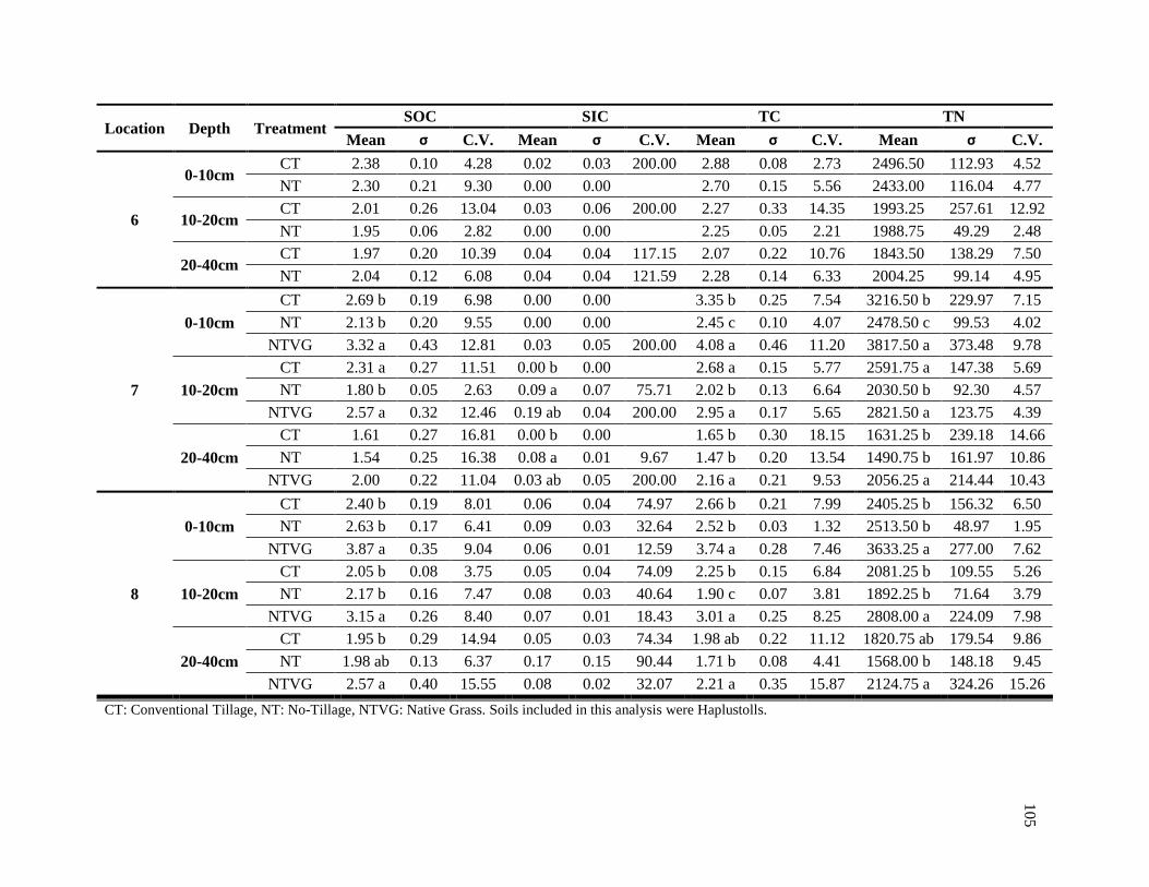
Location Depth Treatment SOC SIC TC TN

Mean σ C.V. Mean σ C.V. Mean σ C.V. Mean σ C.V.

6

0-10cm CT 2.38 0.10 4.28 0.02 0.03 200.00 2.88 0.08 2.73 2496.50 112.93 4.52

NT 2.30 0.21 9.30 0.00 0.00 2.70 0.15 5.56 2433.00 116.04 4.77

10-20cm CT 2.01 0.26 13.04 0.03 0.06 200.00 2.27 0.33 14.35 1993.25 257.61 12.92

NT 1.95 0.06 2.82 0.00 0.00 2.25 0.05 2.21 1988.75 49.29 2.48

20-40cm CT 1.97 0.20 10.39 0.04 0.04 117.15 2.07 0.22 10.76 1843.50 138.29 7.50

NT 2.04 0.12 6.08 0.04 0.04 121.59 2.28 0.14 6.33 2004.25 99.14 4.95

7

0-10cm

CT 2.69 b 0.19 6.98 0.00 0.00 3.35 b 0.25 7.54 3216.50 b 229.97 7.15

NT 2.13 b 0.20 9.55 0.00 0.00 2.45 c 0.10 4.07 2478.50 c 99.53 4.02

NTVG 3.32 a 0.43 12.81 0.03 0.05 200.00 4.08 a 0.46 11.20 3817.50 a 373.48 9.78

10-20cm

CT 2.31 a 0.27 11.51 0.00 b 0.00 2.68 a 0.15 5.77 2591.75 a 147.38 5.69

NT 1.80 b 0.05 2.63 0.09 a 0.07 75.71 2.02 b 0.13 6.64 2030.50 b 92.30 4.57

NTVG 2.57 a 0.32 12.46 0.19 ab 0.04 200.00 2.95 a 0.17 5.65 2821.50 a 123.75 4.39

20-40cm

CT 1.61 0.27 16.81 0.00 b 0.00 1.65 b 0.30 18.15 1631.25 b 239.18 14.66

NT 1.54 0.25 16.38 0.08 a 0.01 9.67 1.47 b 0.20 13.54 1490.75 b 161.97 10.86

NTVG 2.00 0.22 11.04 0.03 ab 0.05 200.00 2.16 a 0.21 9.53 2056.25 a 214.44 10.43

8

0-10cm

CT 2.40 b 0.19 8.01 0.06 0.04 74.97 2.66 b 0.21 7.99 2405.25 b 156.32 6.50

NT 2.63 b 0.17 6.41 0.09 0.03 32.64 2.52 b 0.03 1.32 2513.50 b 48.97 1.95

NTVG 3.87 a 0.35 9.04 0.06 0.01 12.59 3.74 a 0.28 7.46 3633.25 a 277.00 7.62

10-20cm

CT 2.05 b 0.08 3.75 0.05 0.04 74.09 2.25 b 0.15 6.84 2081.25 b 109.55 5.26

NT 2.17 b 0.16 7.47 0.08 0.03 40.64 1.90 c 0.07 3.81 1892.25 b 71.64 3.79

NTVG 3.15 a 0.26 8.40 0.07 0.01 18.43 3.01 a 0.25 8.25 2808.00 a 224.09 7.98

20-40cm

CT 1.95 b 0.29 14.94 0.05 0.03 74.34 1.98 ab 0.22 11.12 1820.75 ab 179.54 9.86

NT 1.98 ab 0.13 6.37 0.17 0.15 90.44 1.71 b 0.08 4.41 1568.00 b 148.18 9.45

NTVG 2.57 a 0.40 15.55 0.08 0.02 32.07 2.21 a 0.35 15.87 2124.75 a 324.26 15.26

CT: Conventional Tillage, NT: No-Tillage, NTVG: Native Grass. Soils included in this analysis were Haplustolls.

105

106

APPENDIX B

107

Supplemental Figure B1: Boxplot illustrating the distribution of soil organic carbon

(SOC) data by different tillage practices. Native conditions were significantly higher in

SOC than any of the cultivated treatments (p<0.0001). There was no significant

difference in Disk/Cultivator, Deep Tillage/Cultivator, or No-Tillage practices. Boxplot

generated in R 3.5.0.

*The top whisker identifies the maximum value of the data, the top of the box represents the third quartile,

the bold black bar represents the median data value, the bottom of the box represents the first quartile, and

the bottom whisker identifies the minimum value of the data.

1 2 3 4

23

45

Soil Organic Carbon x Tillage Practices

Tillage Practice

So

il O

rga

nic

Ca

rbo

n (

%)

b

b

a

1= Disk/Cultivator

2= Deep Tillage/Cultivator

3= No-Till

4= NTVG

b

108

Supplemental Figure B2: Boxplot illustrating the distribution of SOC data by different

crop rotations. Native conditions were significantly higher in SOC than any of the

cultivated crop rotations included in this study (p<0.0001). There was no significant

difference between Corn-Soybean, Corn-Soybean-Oats-Cover Crop, or Continuous Corn

data. Boxplot generated in R 3.5.0.

*The top whisker identifies the maximum value of the data, the top of the box represents the third quartile,

the bold black bar represents the median data value, the bottom of the box represents the first quartile, and

the bottom whisker identifies the minimum value of the data.

1 3 4 5

23

45

Soil Organic Carbon x Crop Rotation

Rotation

So

il O

rga

nic

Ca

rbo

n (

%)

a

b

b

b

1= Corn-Soy

3= Corn-Soy-Oat-Cover Crop

4= Continuous Corn

5= NTVG

109

Supplemental Figure B3: Boxplot illustrating the distribution of SOC data by different

periods of time under No-Till management. When α=0.05, Native Grass (NTVG) had

significantly higher levels of SOC than any of the cultivated treatments. The site that had

been under No-Till (NT) management for 7 years had the least SOC, but was not

significantly different from 4, 10, 21, 26, or 29 years of NT management. In this boxplot,

zero years represent the Conventional Tillage (CT) treatments in this study. Statistically,

CT had the same SOC as 4, 10, 21, 26, and 29 years of NT. Boxplot generated in R 3.5.0.

*The top whisker identifies the maximum value of the data, the top of the box represents the third quartile,

the bold black bar represents the median data value, the bottom of the box represents the first quartile, and

the bottom whisker identifies the minimum value of the data.

0 4 7 10 21 26 29 100

23

45

Soil Organic Carbon by Years of No-Till Management

Years of No-Till Management

So

il O

rga

nic

Ca

rbo

n (

%)

b

0 Years = CT

4 to 29 Years = NT

100 Years = NTVG

bc

c

bc

bc

bc

bc

a

110

Supplemental Figure B4: Boxplot illustrating the distribution of SOC data by Sample

Location. At α=0.05, Location 6 statistically had the least SOC, but was not significantly

different from Locations 4, 7, or 8. Locations 4, 5, 7, and 8 were all statistically similar

for SOC. Locations 1, 2, and 3 had the greatest levels of SOC of all locations in this

study, but were not significantly different from Locations 4, 5, or 8. Boxplot generated

in R 3.5.0.

*The top whisker identifies the maximum value of the data, the top of the box represents the third quartile,

the bold black bar represents the median data value, the bottom of the box represents the first quartile, and

the bottom whisker identifies the minimum value of the data.

1 2 3 4 5 6 7 8

23

45

Soil Organic Carbon by Location

Sample Location

So

il O

rga

nic

Ca

rbo

n (

%)

a

a

a

abc

abc

abc

bc

c

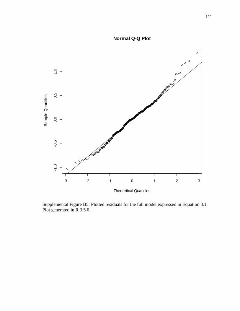
111

Supplemental Figure B5: Plotted residuals for the full model expressed in Equation 3.1.

Plot generated in R 3.5.0.

-3 -2 -1 0 1 2 3

-1.0

-0.5

0.0

0.5

1.0

Normal Q-Q Plot

Theoretical Quantiles

Sa

mp

le Q

ua

ntile

s

112

Supplemental Figure B6: Plotted residuals for the reduced model expressed in Equation

3.3. Plot generated in R 3.5.0.

-3 -2 -1 0 1 2 3

-1.0

-0.5

0.0

0.5

1.0

Normal Q-Q Plot

Theoretical Quantiles

Sa

mp

le Q

ua

ntile

s

113

Supplemental Figure B7: Plotted residuals for the reduced model expressed in Equation

3.4 after Tillage had been removed. Plot generated in R 3.5.0.

-2 -1 0 1 2

-0.4

-0.2

0.0

0.2

0.4

0.6

Normal Q-Q Plot

Theoretical Quantiles

Sa

mp

le Q

ua

ntile

s

114

Supplemental Figure B8: Plotted residuals for the filtered model expressed in Equation

3.5. Plot generated in R 3.5.0.

-2 -1 0 1 2

-0.6

-0.4

-0.2

0.0

0.2

0.4

0.6

Normal Q-Q Plot

Theoretical Quantiles

Sa

mp

le Q

ua

ntile

s

Supplemental Table B1: Example of results for stepwise selection in R 3.5.0. This data refers to the initial reduced model expressed in

Equation 3.3. Model 8 was the model selected for the reduced model due to a high Adjusted R2 and low AIC value.

Subsets Regression Summary

----------------------------------------------------------------------------------------------------------------------------------

Adj. Pred

Model R-Square R-Square R-Square C(p) AIC SBIC SBC MSEP FPE HSP APC

----------------------------------------------------------------------------------------------------------------------------------

1 0.3465 0.3417 0.3316 286.0579 518.6571 -269.1296 533.1387 0.3793 0.3793 0.0014 0.6631

2 0.6207 0.6151 0.6064 53.9137 372.5170 -415.6683 394.2394 0.2226 0.2226 8e-04 0.3877

3 0.6553 0.6490 0.64 26.3106 348.0648 -439.6947 373.4076 0.2037 0.2037 7e-04 0.3548

4 0.6720 0.6647 0.6544 14.1005 336.4063 -450.9945 365.3696 0.1953 0.1953 7e-04 0.3401

5 0.6802 0.6718 0.6609 9.1222 331.4431 -455.6847 364.0267 0.1919 0.1918 7e-04 0.3341

6 0.6852 0.6757 0.6626 6.8589 329.1009 -457.7827 365.3049 0.1903 0.1902 7e-04 0.3312

7 0.6912 0.6807 0.6695 3.6997 325.7532 -460.7589 365.5777 0.1881 0.1879 7e-04 0.3272

8 0.6940 0.6825 0.6697 3.2972 325.2271 -461.0205 368.6719 0.1878 0.1875 7e-04 0.3266 9 0.6954 0.6827 0.6678 4.1026 325.9624 -460.0767 373.0276 0.1883 0.1881 7e-04 0.3275

10 0.6961 0.6822 0.6665 5.5414 327.3663 -458.5007 378.0519 0.1893 0.1890 7e-04 0.3292

11 0.6966 0.6815 0.6656 7.1217 328.9196 -456.7797 383.2256 0.1905 0.1901 7e-04 0.3310

12 0.6966 0.6804 0.6611 9.0401 330.8326 -454.7277 388.7590 0.1919 0.1914 7e-04 0.3333

13 0.6967 0.6792 0.6593 11.0165 332.8075 -452.6192 394.3543 0.1933 0.1928 7e-04 0.3357

14 0.6967 0.6780 0.6576 13.0000 334.7899 -450.5037 399.9571 0.1948 0.1942 7e-04 0.3382

----------------------------------------------------------------------------------------------------------------------------------

AIC: Akaike Information Criteria

SBIC: Sawa's Bayesian Information Criteria

SBC: Schwarz Bayesian Criteria

MSEP: Estimated error of prediction, assuming multivariate normality

FPE: Final Prediction Error

HSP: Hocking's Sp

APC: Amemiya Prediction Criteria

11

5

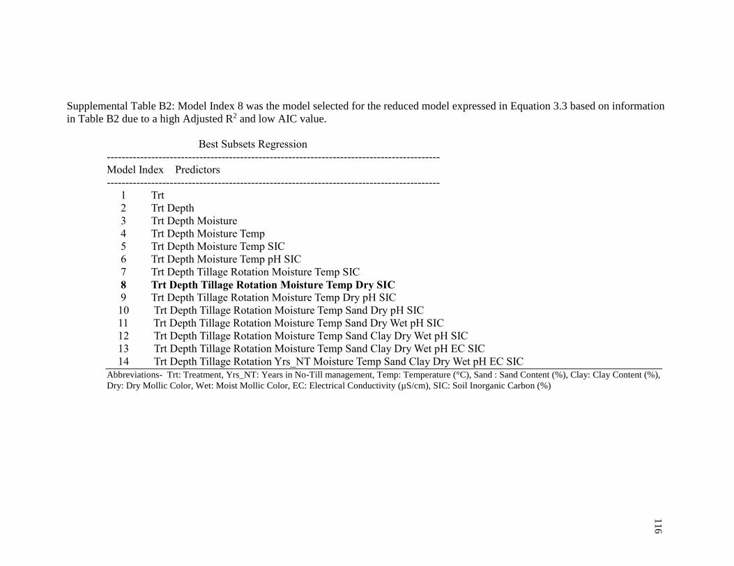
Supplemental Table B2: Model Index 8 was the model selected for the reduced model expressed in Equation 3.3 based on information

in Table B2 due to a high Adjusted R2 and low AIC value.

Best Subsets Regression

------------------------------------------------------------------------------------------

Model Index Predictors

------------------------------------------------------------------------------------------

1 Trt

2 Trt Depth

3 Trt Depth Moisture

4 Trt Depth Moisture Temp

5 Trt Depth Moisture Temp SIC

6 Trt Depth Moisture Temp pH SIC

7 Trt Depth Tillage Rotation Moisture Temp SIC

8 Trt Depth Tillage Rotation Moisture Temp Dry SIC 9 Trt Depth Tillage Rotation Moisture Temp Dry pH SIC

10 Trt Depth Tillage Rotation Moisture Temp Sand Dry pH SIC

11 Trt Depth Tillage Rotation Moisture Temp Sand Dry Wet pH SIC

12 Trt Depth Tillage Rotation Moisture Temp Sand Clay Dry Wet pH SIC

13 Trt Depth Tillage Rotation Moisture Temp Sand Clay Dry Wet pH EC SIC

14 Trt Depth Tillage Rotation Yrs_NT Moisture Temp Sand Clay Dry Wet pH EC SIC

Abbreviations- Trt: Treatment, Yrs_NT: Years in No-Till management, Temp: Temperature (°C), Sand : Sand Content (%), Clay: Clay Content (%),

Dry: Dry Mollic Color, Wet: Moist Mollic Color, EC: Electrical Conductivity (µS/cm), SIC: Soil Inorganic Carbon (%)

11

6