MODELING, SIMULATION, AND VALIDATIONOF CYCLING TIME TRIALS ON REAL

TRACKS

Thorsten Dahmen Roman Byshko Dietmar SaupeUniversity of Konstanz, Konstanz, Germany

Martin RoderND SatCom GmbH, Immenstaad, Germany

Stephan MantlerVRVis Center for Virtual Reality and Visualization Research

Vienna, Austria

Abstract

We develop methods for data acquisition, analysis, modeling and visu-alization of performance parameters in endurance sports with emphasis oncompetitive cycling. For this purpose, we designed a simulator to facilitatethe measurement of training parameters in a laboratory environment, to fa-miliarize cyclists with unknown tracks, and to develop models for trainingcontrol and performance prediction. The simulation includes real height pro-files and a video playback that is synchronized with the cyclist’s current virtualposition on the track and online visualization of various course and perfor-mance parameters. We compared our field data with a the state-of-the artmathematical model for road cycling power, established by Martin et al in1998, which accounts for the gradient force, air resistance, rolling resistance,frictional losses in wheel bearings, and inertia. We found that the model isable to describe the performance parameters accurately. In both cases thecorrelation coefficients were between 0.87–0.95 with signal-to-noise ratios of18–19 dB. We showed that the mathematical model can be implemented on anergometer for simulating rides on real courses. Comparing field and simula-tor measurements we obtained correlation coefficients between 0.66–0.81 withsignal-to-noise ratios of 13–16 dB. The major challenge remains to determinethe model parameters more precisely. Additionally, high quality GPS datawould improve the results.

Keywords: road cycling, performance parameters, mathematical model, simulation,model validation, height profiles.

1

Introduction

Computer science in sports is an emerging interdisciplinary field, which has evolvedin the last 20 to 30 years focussing on the following areas of research: data ac-quisition, processing and analysis, modeling and simulation, data bases and expertsystems, multimedia and presentation, and IT networks/communication. Recordingdevices for a host of physical and physiological parameters have become availableboth to the professional athlete as well as to hobby and amateur sportsmen. Theseparameters are used for monitoring and measuring sports activities in the lab, duringtraining and even in competitions. However, after the data has become available,it still remains difficult to efficiently extract the relevant information. In our workwe contribute to the research aimed at the entire cycle of data acquisition, filtering,analysis, visualization, modeling, and prediction of such complex data. We selectedendurance sports as a particularly suitable application since it allows for long-termdata series that are expected to be more homogeneous, and that depend to a lesserdegree on chance events than, e.g., in game sports. Currently our work focuses onroad cycling, that may later be extended to include, e.g., running and rowing.

For road cycling we develop methods for data acquisition, analysis, modelingand visualization of performance parameters. We designed a simulator to facilitatethe measurement of training parameters in a laboratory environment in addition tomeasuring performance parameters in the field [10]. Several mathematical modelshave been introduced to model road cycling performance, e.g., [4, 7, 8, 9]. Thesemodels were derived from the equilibrium of energy demands and supplies. Thestate-of-the art mathematical model for road cycling power, established by Martinet al in 1998 [7], accounts for the gradient force, air resistance, rolling resistance,frictional losses in wheel bearings and inertia. The models were used to predict timetrial performance [9] and required power output during cycling [7]. Mathematicalperformance models were also used to derive optimal pacing strategies in variablesynthetic terrain and wind conditions [1, 2, 5, 6].

This paper focusses on a comparison of performance parameters in the field, onour lab simulator, and in the mathematical model. Previously, validations of math-ematical models for cycling performance were performed by comparing predictionsof the models to measurements on a flat course. For this study we chose two up-hill tracks with varying steepness. Specifically, the cyclist’s climbing progress onreal outdoor rides on these tracks together with measurements of a power meter iscompared to predictions of the mathematical model for these tracks.

Another contribution of this paper is the comparison between performance pa-rameters measured by the simulator and caculated by the mathematical model. Themain purpose of this task is to provide a means to evaluate the extent to which a labergometer ride can accurately simulate an outdoor ride on real-world tracks. Suchsimulations may then be used by athletes to prepare for competitions on unknowncourses.

In the following subsection we outline the mathematical model for cycling powerthat we used for our comparison with field and lab tests. In the section Methods wediscuss the cycling courses, the equipment, the test setup, the data preprocessing,and the means of comparison of measurements and model prediction. The followingthree sections include the results, their discussion, and conclusions.

2

The mathematical model

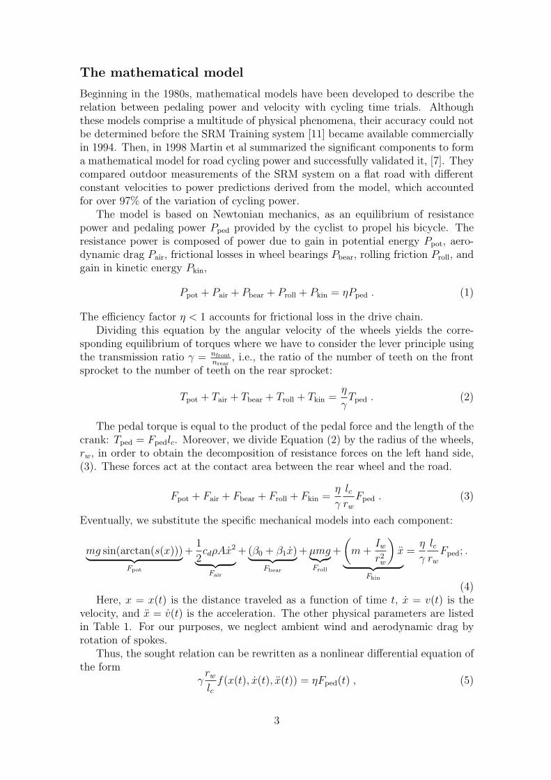
Beginning in the 1980s, mathematical models have been developed to describe therelation between pedaling power and velocity with cycling time trials. Althoughthese models comprise a multitude of physical phenomena, their accuracy could notbe determined before the SRM Training system [11] became available commerciallyin 1994. Then, in 1998 Martin et al summarized the significant components to forma mathematical model for road cycling power and successfully validated it, [7]. Theycompared outdoor measurements of the SRM system on a flat road with differentconstant velocities to power predictions derived from the model, which accountedfor over 97% of the variation of cycling power.

The model is based on Newtonian mechanics, as an equilibrium of resistancepower and pedaling power Pped provided by the cyclist to propel his bicycle. Theresistance power is composed of power due to gain in potential energy Ppot, aero-dynamic drag Pair, frictional losses in wheel bearings Pbear, rolling friction Proll, andgain in kinetic energy Pkin,

Ppot + Pair + Pbear + Proll + Pkin = ηPped . (1)

The efficiency factor η < 1 accounts for frictional loss in the drive chain.Dividing this equation by the angular velocity of the wheels yields the corre-

sponding equilibrium of torques where we have to consider the lever principle usingthe transmission ratio γ = nfront

nrear, i.e., the ratio of the number of teeth on the front

sprocket to the number of teeth on the rear sprocket:

Tpot + Tair + Tbear + Troll + Tkin =η

γTped . (2)

The pedal torque is equal to the product of the pedal force and the length of thecrank: Tped = Fpedlc. Moreover, we divide Equation (2) by the radius of the wheels,rw, in order to obtain the decomposition of resistance forces on the left hand side,(3). These forces act at the contact area between the rear wheel and the road.

Fpot + Fair + Fbear + Froll + Fkin =η

γ

lcrw

Fped . (3)

Eventually, we substitute the specific mechanical models into each component:

mg sin(arctan(s(x)))︸ ︷︷ ︸Fpot

+1

2cdρAx

2︸ ︷︷ ︸Fair

+ (β0 + β1x)︸ ︷︷ ︸Fbear

+µmg︸︷︷︸Froll

+

(m+

Iwr2w

)x︸ ︷︷ ︸

Fkin

=η

γ

lcrw

Fped; .

(4)Here, x = x(t) is the distance traveled as a function of time t, x = v(t) is the

velocity, and x = v(t) is the acceleration. The other physical parameters are listedin Table 1. For our purposes, we neglect ambient wind and aerodynamic drag byrotation of spokes.

Thus, the sought relation can be rewritten as a nonlinear differential equation ofthe form

γrw

lcf(x(t), x(t), x(t)) = ηFped(t) , (5)

3

Cyclist/bicycle/simulatormass cyclist mc Tab. 3mass bicycle mb 10.6 kgtotal mass m mb +mc

simulator inertia I ′ 0.543 kgm2

wheel circumference cw 2100 mmwheel radius rw (2π)−1cwwheel inertia Iw 0.14 kgm2

cross-sectional area A 0.4 m2

length of crank lc 175 mmbearing coefficient β0 0.091 Nbearing coefficient β1 0.0087 Ns/mmechanical gear ratio, bicycle γ 39/26, ..., 53/12fixed gear ratio, simulator γ′ 53/13simulated gear ratio γ′sim 39/26, ..., 53/12

Course/environmentfriction factor µ 0.004gravity factor g 9.81 m/s2

drag coefficient cd 0.7air density ρ 1.2 kg/m3

length L Tab. 2slope s(x) Fig. 1chain efficiency η 0.975

Table 1: Physical parameters of the mathematical model. These parameters orig-inate from our own measurements or were taken from the literature as follows:mc,mb weighted with scales; I ′, lc manufacturer information; cw, L, s(x) measuredusing GPS functionality of Garmin Edge 705 device; Iw, β0, β1, η from [7]; cd, Aaverage value from [12], µ standard value from Cyclus2 for asphalt road.

respectively,f(x(t), x(t), x(t)) · x(t) = ηPped(t) , (6)

where the discounted pedaling force ηFped(t), respectively the discounted pedalingpower ηPped(t), occurs as the driving term for the covered distance x(t), as theindependent variable, and f(x, x, x) denotes the left hand side of Equation (4).

With the mathematical model on hand we used it in two ways.

1. Given the distance measurements x(t) for the duration of a ride, we computedthe corresponding pedaling forces Fped(t), respectively pedaling power Pped, byevaluating f(x(t), x(t), x(t)) in Equation (5). These values were then comparedwith the actual power measurements provided by the SRM.

2. Given measured or prescribed pedaling power Pped(t) for the duration of aride, we solved Equation (6) for x(t) numerically (using MATLAB’s ode45function). The derived values for the velocity v(t) = x(t) were then comparedwith the actual velocity measurements provided by the SRM.

For the model with the simulator, we agree on using primed quantities in thefollowing. Here, the cyclist pedals against the power of the eddy current brake P ′brake,

4

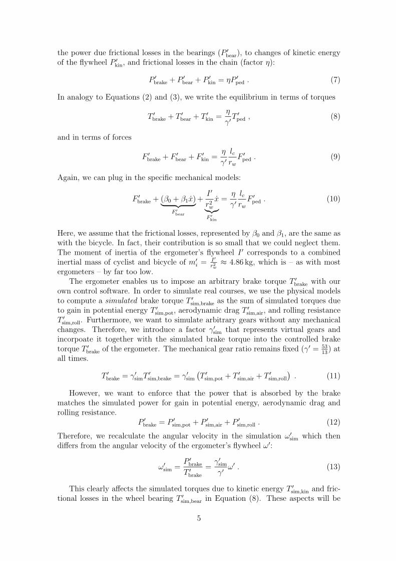
the power due frictional losses in the bearings (P ′bear), to changes of kinetic energyof the flywheel P ′kin, and frictional losses in the chain (factor η):

P ′brake + P ′bear + P ′kin = ηP ′ped . (7)

In analogy to Equations (2) and (3), we write the equilibrium in terms of torques

T ′brake + T ′bear + T ′kin =η

γ′T ′ped , (8)

and in terms of forces

F ′brake + F ′bear + F ′kin =η

γ′lcrw

F ′ped . (9)

Again, we can plug in the specific mechanical models:

F ′brake + (β0 + β1x)︸ ︷︷ ︸F ′

bear

+I ′

r2w

x︸︷︷︸F ′

kin

=η

γ′lcrw

F ′ped . (10)

Here, we assume that the frictional losses, represented by β0 and β1, are the same aswith the bicycle. In fact, their contribution is so small that we could neglect them.The moment of inertia of the ergometer’s flywheel I ′ corresponds to a combinedinertial mass of cyclist and bicycle of m′i = I′

r2w≈ 4.86 kg, which is – as with most

ergometers – by far too low.The ergometer enables us to impose an arbitrary brake torque T ′brake with our

own control software. In order to simulate real courses, we use the physical modelsto compute a simulated brake torque T ′sim,brake as the sum of simulated torques dueto gain in potential energy T ′sim,pot, aerodynamic drag T ′sim,air, and rolling resistanceT ′sim,roll. Furthermore, we want to simulate arbitrary gears without any mechanicalchanges. Therefore, we introduce a factor γ′sim that represents virtual gears andincorpoate it together with the simulated brake torque into the controlled braketorque T ′brake of the ergometer. The mechanical gear ratio remains fixed (γ′ = 53

13) at

all times.

T ′brake = γ′simT′sim,brake = γ′sim

(T ′sim,pot + T ′sim,air + T ′sim,roll

). (11)

However, we want to enforce that the power that is absorbed by the brakematches the simulated power for gain in potential energy, aerodynamic drag androlling resistance.

P ′brake = P ′sim,pot + P ′sim,air + P ′sim,roll . (12)

Therefore, we recalculate the angular velocity in the simulation ω′sim which thendiffers from the angular velocity of the ergometer’s flywheel ω′:

ω′sim =P ′brake

T ′brake

=γ′simγ′

ω′ . (13)

This clearly affects the simulated torques due to kinetic energy T ′sim,kin and fric-tional losses in the wheel bearing T ′sim,bear in Equation (8). These aspects will be

5

subject of a future publication. In the following experiments and computations theyplay only a minor role. With constant velocity, power due to changes in kinetic en-ergy vanishes and in all other model computations for the simulator we accountedfor these effects using Newtonian mechanics. Frictional losses in the wheel bearingsare much smaller than all other components, so we can expect a negligible error if weassume that they are the same for the bicycle, the ergometer and in our simulation.

Methods

Courses

We selected two uphill courses of about 3 km length, with an ascent of about 250 meach and varying steepness, namely the Schiener Berg and Ottenberg, located nearRadolphzell, Germany, and Weinfelden, Switzerland, respectively. See Table 2 andFigures 1–3 for details and picture overviews of the courses. The tracks were recordedby a video camera simultaneously together with the corresponding altitude andGPS tracks with a sampling rate of 1 per second. This allowed us to geo-referenceeach individual video frame. From this alignment we calculated for each frame thedistance traveled from the starting point of the course, the altitude above sea level,and the road gradient. Likewise, for an arbitrary position on the track with a givendistance from the starting point one may calculate a corresponding (fractional) videoframe number for display in the simulation setting [10].

Schiener Berg OttenbergDistance 3630 m 2820 mStart height 429 m 441 mEnd height 674 m 664 mAverage gradient 6.7% 7.9%Maximum gradient 9.7% 13.5%Standard deviation of gradient 1.7% 2.5%

Table 2: Two courses, called Schiener Berg and Ottenberg were chosen for the tests.

Equipment

The riders used the same standard road race bicycle (Radon RPS 9.0 with a 60 cmframe), both in the field and on the simulator. The bicycle has a 10-speed cassette(13–19 and 21, 23, 26 teeth) and is equipped with an SRM power meter with fourstrain gauge strips (Schoberer Rad Messtechnik, Julich, Germany) attached to thechain wheel (53, 39 teeth). Such devices for measuring power are considered state-of-the-art and have been validated in [7]. In our studies, the SRM measurements fordistance travelled, velocity, and power were recorded and used. In addition, otherparameters (heart rate, pedaling frequency) were also recorded but not used here.

Our simulator is based on a Cyclus2 ergometer (RBM Elektronik-AutomationGmbH, Leipzig, Germany). It allows to mount the user’s personal bicycle and hasa flexible front axle attachment, thus, providing a realistic cycling experience, alsowhen riding out of the saddle. The ergometer is governed by an eddy current brake

6

0 500 1000 1500 2000 2500 3000 35000

2

4

6

8

10

12

14

Distance, m

Gra

dien

t, %

0 500 1000 1500 2000 2500 30000

2

4

6

8

10

12

14

Distance, m

Gra

dien

t, %

Figure 1: Gradient versus distance of the courses Schiener Berg (left) and Ottenberg(right). The gradient is smoothed with a Gaussian filter (σ = 30 m).

Figure 2: 3D view of the courses: Schiener Berg (left), Ottenberg (right).

Figure 3: Screenshot of simulation program window. Scene from the Schiener Bergcourse.

7

which can be directly controlled by an external PC-based software at a 2 Hz rate.In the so-called slave mode we can have the ergometer simulated an appropriatebraking action. Our system makes use of this control in order to fully implementthe effects of the actual real-world gradient induced forces, and forces due to aerialdrag, and rolling resistance. Inertial forces and frictional losses in the wheel bearingsare accounted for by the erometer mechanics.

In addition we implemented an option that lets the system set virtual gears ex-actly as given by the 20-speed road bicycle even though the ergometer is designedto accommodate the mechanical gears like those that come with the user’s bicycle.These “soft gears” were necessary because the ergometer is not capable to generatelarge braking forces at low (simulated) velocities, i.e., in low mechanical gears andwith a low back wheel angular velocity, as it would be realistic at the very steep sec-tions of the courses. Instead, a (constant) higher mechanical gear is used throughoutleading to a high angular velocity requiring a prescribed lower than the real brakeforce.

The simulation includes a video playback that is synchronized with the cyclist’scurrent position on the track and online visualization of various course and perfor-mance parameters, namely the time since the start of the ride, the distance travelled,the current velocity, road gradient, pedaling frequency, heart rate, gear ratio, poweroutput, and average power output. Moreover, the height profile for the whole courseand a plot of the gradient near the current position of the rider is shown. This vi-sual feedback was displayed during the simulated rides in the lab using an LCDprojection unit onto a screen of size of about 1 m2. See Figure 3. The details of oursimulation system have been presented at [3] and will be published elsewhere. Asfor the outdoor rides the same parameters were recorded using the mounted SRMchain wheel. Moreover, the Cyclus 2 also provided the measurements of the sameparameters.

Field and simulation tests

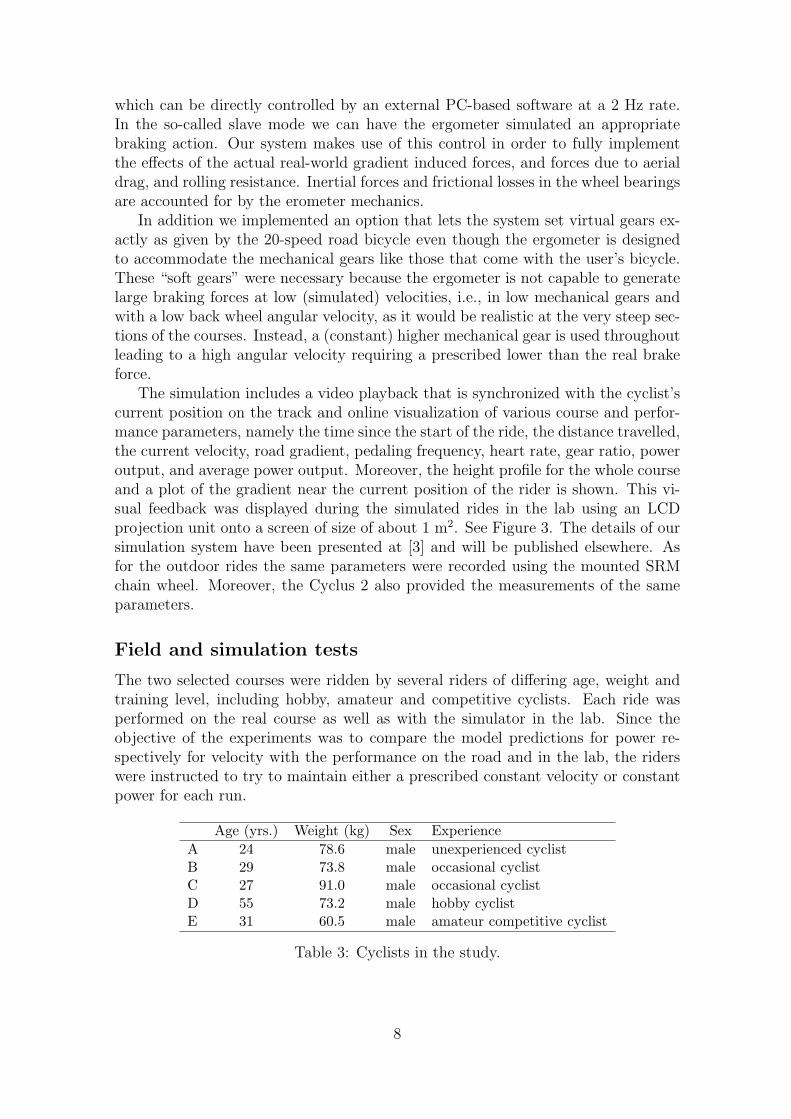
The two selected courses were ridden by several riders of differing age, weight andtraining level, including hobby, amateur and competitive cyclists. Each ride wasperformed on the real course as well as with the simulator in the lab. Since theobjective of the experiments was to compare the model predictions for power re-spectively for velocity with the performance on the road and in the lab, the riderswere instructed to try to maintain either a prescribed constant velocity or constantpower for each run.

Age (yrs.) Weight (kg) Sex ExperienceA 24 78.6 male unexperienced cyclistB 29 73.8 male occasional cyclistC 27 91.0 male occasional cyclistD 55 73.2 male hobby cyclistE 31 60.5 male amateur competitive cyclist

Table 3: Cyclists in the study.

8

Data preprocessing of outdoor measurements

In order to compare the measured power or velocity during an uphill ride withthe corresponding model prediction we needed for each such data the correspondingroad gradient, which was taken from height profiles generated separately. The heightprofiles were measured with a GPS device mounted on a bicycle (a Garmin Edge 705)slowly pushing the bicycle up the hills. The elevation measurement were noisy and,thus, filtered by a Gauss Filter with σ = 30 m. Finally, each elevation was associatedwith the corresponding measured distance from the defined starting point of the ride.

To look up the road gradient for a given point of an actual ride one has totake the distance traveled from the start, look up the corresponding altitudes inthe preprocessed height profiles and estimate a gradient. There are two practicalproblems to carry out this task.

• The distances measured on the rides by the SRM differed slightly from thosein the height profiles. There are several reasons for that. The riders did notride along the exact same path on the road, and, moreover, the distancesmeasured for the height profile had been obtained with a device partly basedon (noisy) GPS data while on the actual rides only wheel revolutions wereautomatically counted and multiplied by the wheel circumference to obtainthe traveled distance.

• The points for the start and end of the tracks were difficult to locate in themeasurement log files because they cannot be exactly marked by the riderswhen passing them.

To solve both problems jointly, we propose to scale and translate the height profileto match the measured distances. We did this manually with a computer program asfollows. Two parameters, namely the start and end position in the log data, had tobe searched for. We identified them by the best match of the measured power curveswith the corresponding predicted power curve of the mathematical model, which wasobtained by visual comparison together with computed correlation coefficients. Thisworked for both types of rides, i.e., with constant velocity and with constant power.In the second case we could compare the measured velocity with the velocity that themodel predicts using the measured power. This semi-automatic procedure providedgood results. We thus refrained from an automated correlation analysis to determineoptimal start and end positions.

Comparison of measurements with model prediction

As result of the preprocessing of the data measured in the field we achieved timeseries of vectors with the components: time t, distance x(t), velocity x(t), powerPped(t), and gradient s(x(t)). For evaluating the rides with constant velocity, thesevalues (except Pped(t)), inserted in the left side of the model equation (6), yield thepredicted power for comparison with the measured power. In the Results sectionbelow we provide corresponding graphs and give correlation coefficients and signal-to-noise ratios (SNR). The latter are defined as

SNR = 10 log10

MSPped

MSEdB (14)

9

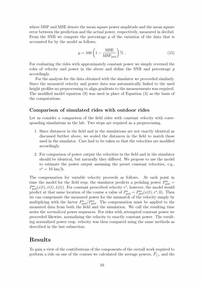
where MSP and MSE denote the mean square power amplitude and the mean squareerror between the prediction and the actual power, respectively, measured in decibel.From the SNR we compute the percentage p of the variation of the data that isaccounted for by the model as follows,

p = 100

(1− MSE

MSPped

)% . (15)

For evaluating the rides with approximately constant power we simply reversed theroles of velocity and power in the above and define the SNR and percentage paccordingly.

For the analysis for the data obtained with the simulator we proceeded similarly.Since the measured velocity and power data was automatically linked to the usedheight profiles no preprocessing to align gradients to the measurements was required.The modified model equation (9) was used in place of Equation (3) as the basis ofthe computations.

Comparison of simulated rides with outdoor rides

Let us consider a comparison of the field rides with constant velocity with corre-sponding simulations in the lab. Two steps are required as a preprocessing.

1. Since distances in the field and in the simulations are not exactly identical asdiscussed further above, we scaled the distances in the field to match thoseused in the simulator. Care had to be taken so that the velocities are modifiedaccordingly.

2. For comparison of power output the velocities in the field and in the simulatorshould be identical, but naturally they differed. We propose to use the modelto estimate the power output assuming the preset constant velocities, e.g.,v? = 10 km/h.

The compensation for variable velocity proceeds as follows. At each point intime the model for the field resp. the simulator predicts a pedaling power Pm

ped =Pm

ped(x(t), x(t), x(t)). For constant prescribed velocity v?, however, the model wouldpredict at that same location of the course a value of P ?

ped = Pmped(x(t), v?, 0). Then

we can compensate the measured power for the mismatch of the velocity simply bymultiplying with the factor P ?

ped/Pmped. The compensation must be applied to the

measured data from both the field and the simulation. We call the resulting timeseries the normalized power sequences. For rides with attempted constant power weproceeded likewise, normalizing the velocity to exactly constant power. The result-ing normalized power resp. velocity was then compared using the same methods asdescribed in the last subsection.

Results

To gain a view of the contributions of the components of the overall work required toperform a ride on one of the courses we calculated the average powers, P(·), and the

10

corresponding fractions that account for gain in potential energy Ppot, aerodynamicdrag Pair, frictional losses in wheel bearings Pbear, rolling friction Proll, and gain inkinetic energy Pkin. For our lightest rider (rider E) at the highest approximatelyconstant velocity (v? = 17 km/h) on the Schiener Berg the average power was 253.8 W,which was distributed as given in Table 4. The total work was 54.2 Wh. It is clearthat the fraction due to overcoming the potential energy Ppot is dominant while theothers are small or even neglectable (Pbear). The average power due to changes ofkinetic energy vanishes perfectly. For other (heavier) riders and for lower velocitythe fraction for overcoming potential energy on this course was even higher.

Power Average power PercentagePpot 222.3 W 87.6%Pair 17.7 W 7.0%Pbear 0.6 W 0.2%Proll 13.2 W 5.2%Pkin 0.0 W 0.0%total 253.8 W 100.0%

Table 4: Distribution of power for a ride up Schiener Berg (3.63 km, 245 m altitude)at 17 km/h requiring a total time of 12 min 49 s and a total energy of 52.4 Wh.

In order to present the main results we chose four bicycle rides that are represen-tative and cover different subjects, courses and pacing strategies out of the 17 thatwere obtained both outdoors on a real course and indoors on the simulator usingthe same course and pacing. Three of these selected rides were performed with ap-proximately constant velocity v? and power was computed using the model. For thefourth one, having approximately constant power P ?, the velocity was computed. Ineach case we plotted the computed quantity against the measurement data. Figures4, 5, and 6 show field measurements and model prediction, simulator measurementsand model prediction, and normalized field and simulator measurements, respec-tively. The Tables 5–7 characterize the deviations of the model predictions fromthe measurements by giving the correlation coefficient ρ, the mean error me, thestandard deviation of the error σe, the SNR as defined in (14), and the percentagep as defined in (15).

Discussion

We organize the discussion in three parts: the comparison of the model predictionswith the measurements in the field, with those in the lab, and the comparison ofthe performance in the field with that in the lab.

Comparison of measurements in the field with modelpredictions

The results in Figure 4 and Table 5 show that the mathematical model describesthe dynamics of power output on an uphill course with good precision. The signal-to-noise ratio was 18–19 dB, which means that 98 to 99% of the variation of the

11

0 500 1000 1500 2000 2500 3000 3500 40000

100

200

300

Distance / m

Pow

er /

W

a) Schiener Berg, Subject A, v = 10 km/h

Model SRM

0 500 1000 1500 2000 2500 3000 3500 4000

100

200

300

400

Distance / m

Pow

er /

W

b) Schiener Berg, Subject E, v = 17 km/h

Model SRM

0 500 1000 1500 2000 2500 30000

100

200

300

400

Distance / m

Pow

er /

W

c) Ottenberg, Subject B, v = 10 km/h

Model SRM

0 500 1000 1500 2000 2500 3000

10

15

20

25

Distance / m

Vel

ocity

/ km

/h

d) Ottenberg, Subject D, P = 250 W

Model SRM

Figure 4: Field rides versus model predictions. The solid line in each plot gives thepower resp. velocity prediction of the model. The prediction errors are analyzed inTable 5.

12

0 500 1000 1500 2000 2500 3000 3500 40000

50

100

150

200

250

300

Distance / m

Pow

er /

W

a) Schiener Berg, Subject A, v = 10 km/h

Model Simulator

0 500 1000 1500 2000 2500 3000 3500 400050

100

150

200

250

300

350

400

Distance / m

Pow

er /

W

b) Schiener Berg, Subject E, v = 17 km/h

Model Simulator

0 500 1000 1500 2000 2500 30000

50

100

150

200

250

300

350

Distance / m

Pow

er /

W

c) Ottenberg, Subject B, v = 10 km/h

Model Simulator

0 500 1000 1500 2000 2500 3000

10

15

20

Distance / m

Vel

ocity

/ km

/h

d) Ottenberg, Subject D, P = 250 W

Model Simulator

Figure 5: Simulated rides versus model. The solid line in each plot gives the powerresp. velocity prediction of the model. The prediction errors are analyzed in Table 6.

13

0 500 1000 1500 2000 2500 3000 3500 40000

50

100

150

200

250

300

350

Distance / m

Pow

er /

W

a) Schiener Berg, Subject A, v = 10 km/h

SRM Simulator

0 500 1000 1500 2000 2500 3000 3500 4000

100

200

300

400

500

Distance / m

Pow

er /

W

b) Schiener Berg, Subject E, v = 17 km/h

SRM Simulator

0 500 1000 1500 2000 2500 30000

50

100

150

200

250

300

350

400

Distance / m

Pow

er /

W

c) Ottenberg, Subject B, v = 10 km/h

SRM Simulator

0 500 1000 1500 2000 2500 30005

10

15

20

25

Distance / m

Vel

ocity

/ km

/h

d) Ottenberg, Subject D, P = 250 W

SRM Simulator

Figure 6: Field versus simulator rides (for normalized measurements). The differ-ences between real-world and simulator rides are analyzed in Table 7.

14

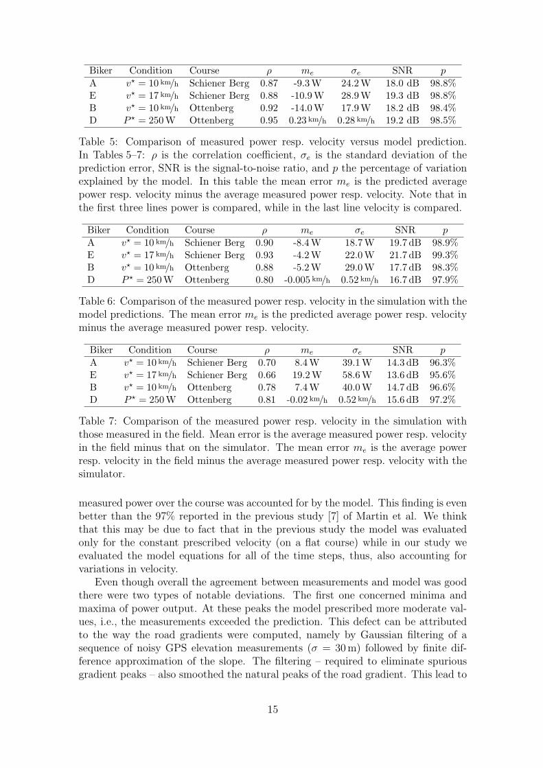
Biker Condition Course ρ me σe SNR p

A v? = 10 km/h Schiener Berg 0.87 -9.3 W 24.2 W 18.0 dB 98.8%E v? = 17 km/h Schiener Berg 0.88 -10.9 W 28.9 W 19.3 dB 98.8%B v? = 10 km/h Ottenberg 0.92 -14.0 W 17.9 W 18.2 dB 98.4%D P ? = 250 W Ottenberg 0.95 0.23 km/h 0.28 km/h 19.2 dB 98.5%

Table 5: Comparison of measured power resp. velocity versus model prediction.In Tables 5–7: ρ is the correlation coefficient, σe is the standard deviation of theprediction error, SNR is the signal-to-noise ratio, and p the percentage of variationexplained by the model. In this table the mean error me is the predicted averagepower resp. velocity minus the average measured power resp. velocity. Note that inthe first three lines power is compared, while in the last line velocity is compared.

Biker Condition Course ρ me σe SNR p

A v? = 10 km/h Schiener Berg 0.90 -8.4 W 18.7 W 19.7 dB 98.9%E v? = 17 km/h Schiener Berg 0.93 -4.2 W 22.0 W 21.7 dB 99.3%B v? = 10 km/h Ottenberg 0.88 -5.2 W 29.0 W 17.7 dB 98.3%D P ? = 250 W Ottenberg 0.80 -0.005 km/h 0.52 km/h 16.7 dB 97.9%

Table 6: Comparison of the measured power resp. velocity in the simulation with themodel predictions. The mean error me is the predicted average power resp. velocityminus the average measured power resp. velocity.

Biker Condition Course ρ me σe SNR p

A v? = 10 km/h Schiener Berg 0.70 8.4 W 39.1 W 14.3 dB 96.3%E v? = 17 km/h Schiener Berg 0.66 19.2 W 58.6 W 13.6 dB 95.6%B v? = 10 km/h Ottenberg 0.78 7.4 W 40.0 W 14.7 dB 96.6%D P ? = 250 W Ottenberg 0.81 -0.02 km/h 0.52 km/h 15.6 dB 97.2%

Table 7: Comparison of the measured power resp. velocity in the simulation withthose measured in the field. Mean error is the average measured power resp. velocityin the field minus that on the simulator. The mean error me is the average powerresp. velocity in the field minus the average measured power resp. velocity with thesimulator.

measured power over the course was accounted for by the model. This finding is evenbetter than the 97% reported in the previous study [7] of Martin et al. We thinkthat this may be due to fact that in the previous study the model was evaluatedonly for the constant prescribed velocity (on a flat course) while in our study weevaluated the model equations for all of the time steps, thus, also accounting forvariations in velocity.

Even though overall the agreement between measurements and model was goodthere were two types of notable deviations. The first one concerned minima andmaxima of power output. At these peaks the model prescribed more moderate val-ues, i.e., the measurements exceeded the prediction. This defect can be attributedto the way the road gradients were computed, namely by Gaussian filtering of asequence of noisy GPS elevation measurements (σ = 30 m) followed by finite dif-ference approximation of the slope. The filtering – required to eliminate spuriousgradient peaks – also smoothed the natural peaks of the road gradient. This lead to

15

the observed smaller model predictions of power at real gradient maxima and largerpredictions at minima.

The other notable deviation of the measurements from the model predictionswas the large mean error of the predictions, negative for power predictions, andpositive for velocity predictions. We believe that this defect may be due to severalfactors: the physical model parameters may not be sufficiently precise. Some weretaken from the literature and should be adapted for our bicycle, the courses, and theriders. Others were measured with errors. Moreover, the model may be incomplete,e.g., we ignored wind effects.

Comparison of simulator measurements with modelpredictions

As above for field measurements we have that also the measurements of power andvelocity on the simulator agreed well with the mathematical model predictions witha signal-to-noise-ratio ranging from about 17 to 22 dB, see Figure 5 and Table 6.As before, we clearly note differences near peaks and a significant negative meanerror of predicted power output. However, in contrast to the above the causes forthese artifacts should be explained differently. This is because we cannot blameinsufficiencies of the mathematical model for imprecise model predictions since it isthe model itself which was implemented in the simulator.

Firstly, unlike above, here we note that the predicted power peaks were morepronounced than the measured ones and not the other way around. We believe thatthis artifact is due to an insufficiency of the eddy current brake of the ergometer torapidly react to changing demand in order to produce the required highly variablebraking power.

Secondly, the mean error was smaller in magnitude than the error for power pre-dictions in the field, but not equal to zero as expected. This led us to the conjectureof a systematic positive bias in the power as given by the simulator. In order to testthis hypothesis, we compared the power measurements of the Cyclus 2 ergometerwith those obtained by the SRM system by mounting our bicycle equipped with theSRM system on the ergometer. For example with rider B on the Ottenberg withv? = 10 km/h we obtained a mean power of 195.2 W as measured by the simulator,which was on average 6.5 W larger than that simultaneously measured by the SRM(standard deviation was 10.7 W). This clearly confirms our conjecture, as, in fact,the outcome should have been reverse, because the power measured by the SRM atthe chain wheel should be larger than that applied to the rear wheel accounting forthe losses in the chain and drive system of the bicycle corresponding to the chainefficiency factor η = 0.975, see Table 1.

Comparison of simulated rides with outdoor rides

Overall, the performance parameters in the simulations were very similar to thosein the field, with a deviation of still 13–15 dB in SNR. See the curves in Figure 6and Table 7. However, since the SRM power measurements in the field had strongerpeaks than the modeled power, which in turn had stronger peaks than the powermeasurements of the simulator, peaks of field and simulator power measurements

16

differed more strongly. Thus, the variation in power on the simulator was lesspronounced than in the field.

Conclusions and future work

In this study we confirmed that a mathematical model for performance parametersin road cycling is capable of accurately predicting required power output also onuphill courses with variable road gradients given the location and velocity alongwith physical, mechanical, and geographical parameters. Alternatively, the modelcan accurately predict velocity of the cyclist given the power applied at the chainwheel.

We showed that the mathematical model can be implemented on an ergometerfor simulated rides on real courses. To a good extent but with certain restrictionsthe simulation was accurate in modeling the performance parameters on the realcourses.

Our study has some limitations; it incorporated (also steep) slopes, but nothigh velocities, which would test for accuracy of the model regarding higher orderterms of the velocity. It did not consider hilly terrain including downhill sections.Furthermore, our results were limited by the accuracy of the required gradients ofthe courses, which were obtained from noisy GPS elevation data, and by the qualityof the other physical and physiological parameters of the mathematical model suchas, e.g., the cross-sectional area of a rider.

We conclude the paper with suggested future work. To obtain more accurateroad gradients we will consider better estimation methods from noisy elevation datasuch as Kalman filtering. Also the quality of the elevation data can be improvedby more accurate measurements using differential GPS or, beginning in 2010, bythe new European satellite navigation system Galileo. Alternatively, commerciallyavailable airborne laser scanned elevation data may be used.

To derive improved parameters for the mathematical model we will consider anindirect method. Based on measurements of location, power, and velocity duringlonger rides over variable terrain we propose to fit the parameters of a generalizedmodel to that data. As a result, we will obtain parameters that act, e.g., as factorsfor the linear and quadratic terms in the model rather than a complete list of phys-ical parameters. Moreover, in this way we may be able to improve the model byincorporating higher order terms that are not accounted for in the current model.

To improve the operation of our simulator we may redesign its computer controlsuch that the power given by the mathematical model as required at the chain wheelmust actually be provided by the rider. This may be achieved by a training procedureto be developed using a feedback loop that includes the SRM measurements at thechain wheel as a control mechanism.

Future work includes measuring also wind direction and velocity both on groundand on the bicycle, simulator rides on terrain with mild hills, so that the downhillparts do not violate the simulator design, i.e, the simulator must still generate abraking force (due to air drag).

We also strive to use the model to find the optimum pacing strategy as Maronski,1994 [6], Gordon, 2005 [5], and Atkinson, 2007 [2], recently discussed for simple hy-

17

pothetic height profiles. Together with an extension of physiological measurementsand their modeling the whole system shall indicate and train effective tactics us-ing sophisticated biofeedback visualization and enable cyclists to optimally preparethemselves even for unfamiliar tracks.

Acknowledgments: This research was supported by the DFG Research TrainingGroup GRK 1042, “Explorative Analysis and Visualization of Large InformationSpaces”. We thank Dr. Dietmar Luchtenberg of the Department of Sport Scienceof the University of Konstanz for discussions and support. A part of this workwas carried out while the third author was a Visiting Research Fellow at RSISE,Australian National University, Canberra, whose support is gratefully acknowledged.

References

[1] G. Atkinson and A. Brunskill. Pacing strategies during a cycling time trial withsimulated headwinds and tailwinds. Ergonomics, 43(10):1449–1460, 2000.

[2] G. Atkinson, O. Peacock, and L. Passfield. Variable versus constant powerstrategies during cycling time-trials: Prediction of time savings using an up-to-date mathematical model. Journal of Sports Sciences, 25(9):1001–1009, 2007.

[3] T. Dahmen and D. Saupe. A simulator for race-bike training on real tracks.In S. Loland, K. Bø, K. Fasting, J. Halln, Y. Ommundsen, G. Roberts, andE. Tsolakidis, editors, 14th annual Congress of the European College of SportScience, Oslo/Norway, June 2009.

[4] P. E. di Prampero, G. Cortili, P. Mognoni, and F. Saibene. Equation of motionof a cyclist. J Appl Physiol, 47(1):201–206, July 1979.

[5] S. Gordon. Optimising distribution of power during a cycling time trial. SportsEngineering, 8(2):81–90, 2005.

[6] R. Maronski. On optimal velocity during cycling. J Biomech, 27(2):205–213,Feb 1994.

[7] J. C. Martin, Douglas L. Milliken, John E. Cobb, Kevin L. McFadden, andAndrew R. Coggan. Validation of a mathematical model for road cycling power.Journal of Applied Biomechanics, 14:276–291, 1998.

[8] T. S. Olds, K. I. Norton, and N. P. Craig. Mathematical model of cyclingperformance. J Appl Physiol, 75(2):730–737, Aug 1993.

[9] T. S. Olds, K. I. Norton, E. L. Lowe, S. Olive, F. Reay, and S. Ly. Modelingroad-cycling performance. J Appl Physiol, 78(4):1596–1611, Apr 1995.

[10] D. Saupe, D. Luchtenberg, M. Roder, and C. Federolf. Analysis and visual-ization of space-time variant parameters in endurance sports training. In Pro-ceedings of the 6th International Symposium on Computer Science in Sports(IACSS 2007), 2007.

18

[11] E Schoberer. Operating instructions for the srm training system.http://www.srm.de/index.php?option=com phocadownload&view=sections&Itemid=248&lang=en.

[12] David Gordon Wilson. Bicycling Science, 3rd Edition. The MIT Press, 3edition, April 2004.

19