Modeling Route Choice Behavior Using Stochastic Learning Automata

Paper No. 01-0372

Duplication for publication or sale is strictly prohibited without prior written permission

of the Transportation Research Board

Title: Modeling Route Choice Behavior Using Stochastic Learning Automata

Authors: Kaan Ozbay, Aleek Datta, Pushkin Kachroo

Transportation Research Board 80th Annual Meeting January 7-11, 2001 Washington, D.C.

Ozbay, Datta, Kachroo 1

MODELING ROUTE CHOICE BEHAVIOR USING STOCHASTIC LEARNING AUTOMATA

By

Kaan Ozbay, Assistant Professor Department of Civil & Environmental Engineering

Rutgers, The State University of New Jersey Piscataway, NJ 08854-8014

Aleek Datta, Research Assistant

Department of Civil & Environmental Engineering Rutgers, The State University of New Jersey

Piscataway, NJ 08854-8014

Pushkin Kachroo, Assistant Professor Bradley Department of Electrical & Computer Engineering

Virginia Polytechnic Institute and State University Blacksburg, VA 24061

ABSTRACT

This paper analyzes day-to-day route choice behavior of drivers by introducing a new route choice model developed using stochastic learning automata (SLA) theory. This day-to-day route choice model addresses the learning behavior of travelers based on experienced travel time and day-to-day learning. In order to calibrate the penalties of the model, an Internet based Route Choice Simulator (IRCS) was developed. The IRCS is a traffic simulation model that represents within day and day-to-day fluctuations in traffic and was developed using Java programming. The calibrated SLA model is then applied to a simple transportation network to test if global user equilibrium, instantaneous equilibrium, and driver learning have occurred over a period of time. It is observed that the developed stochastic learning model accurately depicts the day-to-day learning behavior of travelers. Finally, it is shown that the sample network converges to equilibrium, both in terms of global user and instantaneous equilibrium. Key Words: Route Choice Behavior, Travel Simulator, Java


1.0 INTRODUCTION & MOTIVATION

In recent years, engineers have foreseen the use of advanced traveler information systems (ATIS),

specifically route guidance, as a means to reduce traffic congestion. Unfortunately, experimental

data that reflects traveler response to route guidance is not available in abundance. Especially,

effective models of route choice behavior that capture the day-to-day learning behavior of drivers

are needed to estimate traveler response to information, to engineer ATIS systems, and to evaluate

them as well. Extensive data is required for developing the route choice models necessary to

provide understanding of traveler response to traffic conditions. Route guidance by providing

traffic information can be a useful solution only if drivers’ route choice and learning behavior is

well understood.

As a result of these developments and needs in the area of ATIS, several researchers have been

recently working on the development of realistic route choice models with or without a learning

component. Most of the previous work uses the concept of "discrete choice models" for modeling

user choice behavior. The discrete choice modeling approach is a very useful one except for the

fact that it requires accurate and quite large data sets for the estimation and calibration of driver

utility function. Moreover, there is no direct proof that drivers make day-to-day route choice

decisions based on the utility functions. Due to the recognition of these and other difficulties in

developing, calibrating, and subsequently justifying the use of the existing approaches for route

choice, we propose the use of an "artificial intelligence" type of approach, namely stochastic

learning automata (SLA) (Narendra 1988).

The concept of learning automaton grew from a fusion of the work of psychologists in modeling

observed behavior, the efforts of statisticians to model the choice of experiments based on past

observations, and the efforts of system engineers to make random control and optimization

decisions in random environments.

In the case of "route choice behavior modeling", which also occurs in a stochastic environment,

stochastic learning automata mimics the day-to-day learning of drivers by updating the route

choice probabilities based on the basis of information received and the experience of drivers. Of

course the appropriate selection of the proper learning algorithm as well as the parameters it

contains is crucial for its success in modeling user route choice behavior.


This paper attempts to introduce a new route choice model by modeling route choice behavior

using stochastic learning automata theory that is widely used in biological and engineering systems.

This route choice model addresses the learning behavior of travelers based on experienced travel

times (day-to-day learning). In simple terms, the stochastic learning automata approach adopted in

this paper is an inductive inference mechanism which updates the probabilities of its actions

occurring in a stochastic environment in order to improve a certain performance index, i.e. travel

time of users.

2.0 LITERATURE REVIEW

According to the underlying hypothesis of discrete choice models, an individual’s preferences for

each alternative when faced with a set of choices (routes or modes) can be represented by using a

utility measure. This utility measure is assumed to be a function of the attributes of the

alternatives as well as the decision maker’s characteristics. The decision maker is assumed to

choose the alternative with the highest utility. The utility of each alternative to a specific decision

maker can be expressed as a function of observed attributes of the available alternatives and the

relevant observed characteristics of the decision maker (Sheffi, 1985). Now, let a denote the vector

of variables which includes these attributes and characteristics, and let the utility function be

denoted as ( ak V k ) = V k = Utility Function .

The distribution of the utilities is a function of this attribute vector a. Therefore the probability

that alternative k will be chosen, Pk can be related to a using the widely used “multinomial logit”

(MNL) choice model and of the following form (Sheffi, 1985):

P k = e V k

e V l l = 1

Κ ∑

∀ k ∈ Κ (1)

P k = P k ( ak ) = Choice Function

Pk has all the properties of an element of a probability mass function, that is,

0 ≤ P k ( ak ) ≤ 1 ∀ k ∈ Κ

P k ( ak ) = 1 k = 1

Κ ∑

(2)


In a recent paper by Vaughn et al. (1996), a general multinomial choice for route choice under

ATIS is given. The utility function Vk can be expressed in the functional form:

V = f(Individual characteristics, Route specific characteristics, Expectations, Information, Habit

persistence)

The variables in each group are (Vaughn et al., 1996):

• Individual characteristics: gender, age level, and education level.

• Route specific attributes: number of stop locations on route.

• Expectations: expected travel time, standard deviation of the expected travel time, expected

stop time.

• Information: incident information, congestion information, pre-trip information.

• Habit: Habit persistence, or habit strength.

For the base model, a simple utility function of the following form is used:

))ß(E(tt a V ijtijt += i (3)

where,

Vijt = expected utility of route j on day t for individual i

E(ttijt) = expected travel time on route j on day t for individual i

α j = route specific constant

Several computer-based experiments have recently been conducted to produce route choice models.

Iida, Akiyama, and Uchida (1992) developed a route choice model based on actual and predicted

travel times of drivers. Their model of route choice behavior is based upon a driver’s traveling

experience. During the course of the experiment, each driver was asked to predict travel times for

the route to be taken (1 O-D pair only), and after the route was traveled, the actual travel time was

displayed. Based on this knowledge, the driver was asked to repeat this procedure for several

iterations. However, the travel time on the alternative route was not given to the driver, and the

driver was not allowed to keep records of past travel times. In a second experiment, the driver was

asked to perform the same tasks, but was allowed to keep records of the travel times. Two models

were developed, one for each experiment. The actual and predicted travel times for route r for the

i-th participant and the n-th iteration are defined as nrit , n

rit̂ , respectively, and the predicted travel

time on the route r for the n + 1-th iteration, 1+nrit , is corrected based on the n-th iterations actual


travel time and its deviation from the predicted travel time for that iteration. The travel time

prediction model for the second case is as follows:

3 31201 xxxy βββα +++= (4)

where, nri

nri

knri

knrik ttyttx ˆ , - ˆ 1 −== +−− (5)

The parameters β1, β2, and β3 are regression coefficients. X is the difference between the actual

and predicted travel times of the i-th participant for the n-th iteration, and y represents the

adjusting factor for the n+1-th iteration’s predicted travel time from the n-th iteration’s actual

travel time.

Another route choice model developed by Nakayama and Kitamura (1999) assumes that drivers

“reason and learn inductively based on cognitive psychology”. The model system is a compilation

of “if-then” statements in which the rules governing the statements are systematically updated

using algorithms. In essence, the model system represents route choice by a set of rules similar to

a production system. The rules for the system represent various cognitive processes. If more than

one “if-then” rule applies to a given situation, then the rule that has provided the best directions in

the past holds true. The “strength indicator” of each rule is a weighted average of experienced

travel times.

Mahmassani and Chang developed a framework to describe the processes governing commuter’s

daily departure time decisions in response to experienced travel times and congestion. It was

determined that commuter behavior can be viewed as a “boundedly-rational” search for an

accepted travel time. Results indicated that a time frame of tolerable schedule delay existed,

termed an “indifference band”. This band varied among individuals, and was also effected by the

user’s experience with the network.

Jha et. al developed a Bayesian updating model to simulate how travelers update their perceived

day-to-day travel time based on information provided by ATIS systems and their previous

experience. The framework explicitly modeled the availability and quality of traffic information.

They used a disutility function to model driver’s perceived travel time and schedule delay in order

to evaluate alternative travel choices. Eventually, the driver chooses an alternative based on utility

maximization principle. Finally, the both models are incorporated into a traffic simulator.


2.1 LEARNING MECHANISMS IN ROUTE CHOICE MODELING

Generally users cannot foresee the actual travel cost that they will experience during their trip.

However, they do anticipate the cost of their travel based on the costs experienced during their

previous trips of similar characteristics. Hence, learning and forecasting processes for route choice

can be modeled through the use of statistical models applied to path costs experienced on previous

trips. There are different kinds of statistical learning models proposed in Cascetta and Canteralla

(1993) or Davis and Nihan (1993). There are also other learning and forecasting filters that are

empirically calibrated (Mahmassani and Chang, 1985). Most of the previous route choice models

in the literature model the learning and forecasting process using one of the two general approaches

briefly described below (Cascetta and Canteralla, 1995):

• Deterministic or stochastic threshold models based on the difference between the forecasted

and actual cost of the alternative chosen the previous day for switching choice probabilities

(Mahmassani and Chang, 1985).

• Extra utility models for conditional path choice models where the path chosen the previous day

is given an extra utility in order to reflect the transition cost to a different alternative (Cascetta

and Cantarella, 1993).

• Stochastic models that update the probability of choosing a route based on previous

experiences according to a specific rule, such as Bayes’ Rule. Stochastic learning is also the

learning mechanism adopted in this paper with the exception that the SLA learning rule is a

general one and different from Bayes’ rule.

3.0 LEARNING AUTOMATA

Classical control theory requires a fair amount of knowledge of the system to be controlled. The

mathematical model is often assumed to be exact, and the inputs are deterministic functions of

time. Modern control theory, on the other hand, explicitly considers the uncertainties present in the

system, but stochastic control methods assume that the characteristics of the uncertainties are

known. However, all those assumptions concerning uncertainties and/or input functions may not

be valid or accurate. It is therefore necessary to obtain further knowledge of the system by

observing it during operation, since a priori assumptions may not be sufficient.

It is possible to view the problem of route choice as a problem in learning. Learning is defined as a

change in behavior as a result of past experience. A learning system should therefore have the


ability to improve its behavior with time. “In a purely mathematical context, the goal of a learning

system is the optimization of a functional not known explicitly”.

The stochastic automaton attempts a solution of the problem without any a priori information on

the optimal action. One action is selected at random, the response from the environment is

observed, action probabilities are updated based on that response, and the procedure is repeated. A

stochastic automaton acting as described to improve its performance is called a learning

automaton (LA). This approach does not require the explicit development of a utility function

since the behavior of drivers in our case is implicitly embedded in the parameters of the learning

algorithm itself.

The first learning automata models were developed in mathematical psychology. Bush and

Mosteller, 1958, and Atkinson et al., 1965, survey early research in this area. Tsetlin (1973)

introduced deterministic automata operating in random environments as a model of learning. Fu

and colleagues were the first researchers to introduce stochastic automata into the control literature

(Fu, 1967). Recent applications of learning automata to real life problems include control of

absorption columns (Fu, 1967) and bioreactors (Gilbert et al., 1993). Theoretical results on

learning algorithms and techniques can be found in recent IEEE transactions (Najaraman et al.,

1996, Najim et al., 1994) and in Najim-Poznyak collaboration (Najim et al., 1994).

3.1 LEARNING PARADIGM

The automaton can perform a finite number of actions in a random environment. When a specific

action α is performed, the environment responds by producing an environment output β, which is

stochastically related to the action (Figure 1). This response may be favorable or unfavorable (or

may define the degree of “acceptability” for the action). The aim is to design an automaton that

can determine the best action guided by past actions and responses. An important point is that

knowledge of the nature of the environment is minimal. The environment may be time varying, the

automaton may be a part of a hierarchical decision structure but unaware of its role, or the

stochastic characteristics of the output of the environment may be caused by the actions of other

agents unknown to the automaton.


Response

Action α

β

Automaton

Environment

probabilitiesprobabilitiesPenaltyAction

P C

Figure 1. The automaton and the environment

The input action α(n) is applied to the environment at time n. The output β(n) of the environment is

an element of the set β=[0,1] in our application. There are several models defined by the output set

of the environment. Models in which the output can take only one of two values, 0 or 1, are

referred to as P-models. The output value of 1 corresponds to an “unfavorable” (failure, penalty)

response, while output of 0 means the action is “favorable.” When the output of the environment is

a continuous random variable with possible values in an interval [a, b], the model is named S-

model.

The environment where the automaton “lives,” is defined by a triplet {α,c,β} where α is the action

set, β represents a (binary) output set, and c is a set of penalty probabilities (or probabilities of

receiving a penalty from the environment for an action) where each element ci corresponds to one

action αi of the action set α. The response of the environment is considered to be a random

variable. If the probability of receiving a penalty for a given action is constant, the environment is

called a stationary environment; otherwise, it is non-stationary. The need for learning and

adaptation in systems is mainly due to the fact that the environment changes with time.

Performance improvement can only be a result of a learning scheme that has sufficient flexibility to

track the better actions. The aim in these cases is not to evolve to a single action that is optimal,

but to choose actions that minimize the expected penalty. For our application, the (automata)

environment is non-stationary since the physical environment changes as a result of actions taken.

The main concept behind the learning automaton model is the concept of a probability vector

defined (for P-model environment) as

p(n) = {pi (n) ∈{0,1} pi(n) = Pr[α(n) = α i]}


where αi is one of the possible actions. We consider a stochastic system in which the action

probabilities are updated at every stage n using a reinforcement scheme. The updating of the

probability vector with this reinforcement scheme provides the learning behavior of the automata.

3.2 REINFORCEMENT SCHEMES

A learning automaton generates a sequence of actions on the basis of its interaction with the

environment. If the automaton is “learning” in the process, its performance must be superior to an

automaton for which the action probabilities are equal. “The quantitative basis for assessing the

learning behavior is quite complex, even in the simplest P-model and stationary random

environments (Narendra et al., 1989)”. Based on the average penalty to the automaton, several

definitions of behavior, such as expediency, optimality, and absolute expediency, are given in the

literature. Reinforcement schemes are categorized based on the behavior type they provide, and the

linearity of the reinforcement algorithm. Thus, a reinforcement scheme can be represented as:

p(n + 1) = T[p(n),α(n),β(n)], where T is a mapping, α is the action, and β is the input from the

environment. If p(n+1) is a linear function of p(n), the reinforcement scheme is said to be linear;

otherwise it is termed nonlinear. Early studies of reinforcement schemes were centered on linear

schemes for reasons of analytical simplicity. In spite of the efforts of many researchers, a general

algorithm that ensures optimality has not been found (Kushner et al., 1979). Optimality implies

that action αm associated with the minimum penalty probability cm is chosen asymptotically with

probability one. Since, it is not possible to achieve optimality in every given situation, a sub

optimal behavior is defined, where the asymptotic behavior of the automata is sufficiently close to

optimal case.

A few attempts were made to study nonlinear schemes (Chandraeskharan et al.1968, Baba, 1984).

Generalization of such schemes to the action case was not straightforward. Later, researchers

started looking for the conditions on the updating functions that ensure a desired behavior. This

approach led to the concept of absolute expediency. An automaton is said to be absolutely

expedient if the expected value of the average penalty at one iteration step is less than the previous

step for all steps. Absolutely expedient learning schemes are presently the only class of schemes

for which necessary and sufficient conditions of design are available (Chandraeskharan et al.1968,

Baba,1984).


3.3 AUTOMATA AND ENVIRONMENT

The learning automaton may also send its action to multiple environments at the same time. In that

case, the actions of an automaton result in a vector of feedback values from the environment.

Then, the automaton has to “find” an optimal action that “satisfies” all the environments (in other

words, all the “teachers”). In a multi-teacher environment, the automaton is connected to N

separate teachers. The action set of the automaton is of course the same for all

teacher/environments. Baba (1984) discussed the problem of a variable-structure automaton

operating in many-teacher (stationary and non-stationary) environments. Conditions for absolute

expediency are given in his work.

4.0 STOCHASTIC LEARNING AUTOMATA (SLA) BASED ROUTE CHOICE

(RC) MODEL - SLA-RC MODEL

Some of the major advantages of using stochastic learning automata for modeling user choice

behavior can be summarized as follows:

1. Unlike existing route choice models that capture learning process as a deterministic

combination of previous days’ and the current day’s experience, SLA-RC model captures the

learning process as a stochastic one.

2. The general utility function, V(), used by the existing route choice models is a linear

combination of explanatory variables. However, stochastic learning automata can easily

capture non-linear combinations of these explanatory variables (Narendra and Thathnachar,

1989). This presents an important improvement over existing route choice models since in

reality route choice cannot be expected to be a linear combination of the explanatory variables.

4.1 DESCRIPTION OF THE STOCHASTIC LEARNING AUTOMATA ROUTE

CHOICE (SLA-RC) MODEL

This model consists of two components. These are:

• Choice Set: Two types of choice sets can be defined. The first type will be comprised of

complete routes between each origin and destination. The user will choose one of these routes

every day. This is similar to the pre-trip route choice mechanism. The second type can be

comprised of decision points in such a way that the user will choose partial routes to his/her


destination at each of these decision points. This option is similar to the “en-route” decision-

making mechanism.

• Learning Mechanism: The learning process will be modeled using stochastic learning

automata that is described in detail in this section.

Let’s assume that there exists an input set X that is comprised of explanatory variables described

in Vaughn et al. (1996). Thus X={x1,1, x1,2 … . xt,i} where “t” is the day and “i“ is the individual

user or user class. Let’s also assume that there exists an output set D which is comprised of the

decisions of route choices, such that D={d1, d2,.......dj}, where j is the number of acceptable routes.

This simple system is shown in Figure 2. This system can be made into a feedback system where

the effect of user choice on the traffic and vice versa is modeled. This proposed feedback system is

shown in figure 3.

O D

Figure 2. One Origin - One Destination Multiple Route System

Route Choice Probabilities

Traffic Network

Updated Travel Times

Figure 3. Feedback mechanism for the SLA-RCM.

For a very simple case with only two routes between an origin and destination and one user class

exist, the above system can be seen as a double action system. Then, to update the route choice

probability, we can use linear reward-penalty learning scheme proposed in Narendra and

Thathnachar (1989). This stochastic automata based learning scheme is selected due to its

applicability to the modeling of human learning mechanism in the context of route choice process.


4.1.1 LINEAR REWARD-PENALTY (LR -P ) SCHEME

This learning scheme was first used in mathematical psychology. The idea behind a reinforcement

scheme, such as linear reward-penalty (LR -P ) scheme, is a simple one. If the automaton picks an

action α i at instant n and a favorable input β(n) = 0( ) results, the action probability pi(n) is

increased and all other components of p(n) are decreased. For an unfavorable input β(n) = 1,

pi(n) is increased and all other components of p(n) are decreased.

In order to apply this idea to our situation, assume that there are r distinct routes to choose

between an origin-destination pair, as seen in Figure 2. Therefore, we can consider this system as

a variable-structure automaton with r actions to operate in a stationary environment. A general

scheme for updating action probabilities can be represented as follows:

If

α ( n ) = α i ( i = 1 , ..... r )

p j ( n + 1 ) = p j ( n ) − g j [ p ( n )] when β ( n ) = 0

p j ( n + 1 ) = p j ( n ) + h j [ p ( n )] when β ( n ) = 1

for all j ≠ i

(6)

To preserve the probability measure we have p j(n)j =1

r

∑ = 1 so that

pi(n + 1) = pi(n) + g j(p(n))j=1j≠ i

r

∑ when β(n) = 0

pi(n + 1) = pi(n) − h j(p(n))j=1j≠ i

r

∑ when β(n) = 1

(7)

The updating scheme is given at every instant separately for that action which is attempted at stage

n in equation (7) and separately for actions that are not attempted in equation (6). Reasons behind

this specific updating scheme are explained in Narendara and Thathnachar (1989). In the above

equations, the action probability at stage (n + 1) is updated on the basis of its previous value, the

action α(n) at the instant n and the input β(n) . In this scheme, p(n+1) is a linear function of

p(n), and thus, the reinforcement (learning) scheme is said to be linear. If we assume a simple

network with one origin destination pair and two routes between this O-D pair, we can consider a

learning automaton with two actions in the following form:


g j (p(n)) = ap j(n)

andh j(p(n)) = b(1 − p j (n))

(8)

In equation (8) a and b are reward and penalty parameters and 0 < a <1, 0 < b < 1 . If we

substitute (8) in equations (6) and (7), the updating (learning) algorithm for this simple two route

system can be re-written as follows:

p1 (n + 1) = p1(n) + a(1 − p1(n))p2 (n + 1) = (1 − a)p2 (n)

α(n) = α1,β(n) = 0

p1 (n + 1) = (1 − b)p1(n) p2 (n + 1) = p2 (n) + b(1 − p2(n))

α(n) = α1,β(n) = 1

(9)

Equation (9) is in general referred as the general LR -P updating algorithm. From these equations, it

follows that if action α i is attempted at stage n, the probability 1j (n)p ≠j is decreased at stage n+1

by an amount proportional to its value at stage n for a favorable response and increased by an

amount proportional to 1 − p j(n)[ ] for an unfavorable response.

If we think in terms of route choice decisions, if at day n+1, the travel time on route 1 is less than

the travel time on route 2, then we consider this as a favorable response and the algorithm increases

the probability of choosing route 1 and decreases the probability of choosing route 2. However, if

the travel time on route 1 at day n+1 is higher than the travel time on route 2 the same day, then the

algorithm decreases the probability of choosing route 1 and increases the probability of choosing

route 2. In this paper, we do not address “departure time choice” decisions. It is assumed that

each person departs during the same time interval ∆t. It is also assumed that, for this example,

there is one class of user.

5.0. DYNAMIC TRAFFIC / ROUTE CHOICE SIMULATOR

The Internet based Route Choice Simulator (IRCS), shown in Figure 4, is the travel simulator

developed for this project and was based on one O-D pair and two routes. The simulator is a Java

applet designed to acquire data for creating a learning automata model for route choice behavior.

The applet can be accessed from any Java-enabled browser over the Internet. Several advantages

exist in using web-based travel simulators. First, these simulators are easy to access by different


types of subjects. Geographic location does not prevent test subjects from participating in the

experiments. Second, Internet based simulators permit the possibility of having a large number of

subjects partake in the experiment. Internet-based simulators are designed to have a user-friendly

GUI, and reduce confusion amongst subjects. Also, Java-based simulators are not limited by

hardware, such as the computer type, i.e. Mac, PC, UNIX. Any computer using a Java-enabled

web browser can use these simulators. Finally, data processing and manipulation capabilities are

significantly increased when using web-based simulators due to the very effective and on-line

database tools established for Internet applications.

The site hosting this travel simulator consists of an introductory web page that gives a brief

description of the project, and directions on how to properly use the simulator. Following a link on

that page brings the viewer to the applet itself. The applet is intended to simulate route choice

between two alternative routes. Travel time on route i is the result of a random number picked

from a normal distribution with a mean and standard deviation of (µ, σ) and the sum of a nominal

average value for travel time on that route as seen in Equation 10.

Travel_ Time(i) = Fixed_ Travel_ Time + Random_Value(µ,σ) (10)

Users conducting the experiment are asked to make route choice decision on a day-to-day basis.

The simulator shows the user the experienced route travel time for each day. Another method for

determine travel times is by incorporating the effect of choosing the specific route in terms of extra

volume. In this case, travel time is determined as seen in Equation 11.

Travel _ Time ( i ) = f(volume) (11)

The applet can be divided into two sections. The first section is the GUI and the algorithms for

determining travel time on each route. Before beginning the experiment, the participant is asked to

enter personal and socio-economic data such as name, age, gender, occupation, and income, and

user-status. This data will be used in the future to create driver classes and to compare the route

choice behavior and learning curves for various classes. Also included in the data survey section

are choices for purpose of trip, departure time, desired arrival time, and actual arrival time. For

example, if the participant assumed that this experiment simulated a commute from home to work,


then the participant would realize the importance of arriving at the destination as quickly as

possible. Also, the participant could determine how accurate his or her desired arrival time is

compared to the actual arrival time.

Figure 4. GUI of Internet Based Route Choice Simulator (IRCS)

The graphics presently incorporated in the applet are GIS maps of New Jersey. These maps can be

changed to any image to portray any origin-destination pair. Route choices can be made by

clicking on either button on the left panel of the applet. The purpose of having two image panels is

two-fold. First, the larger panel on the left can hold a large map of any size, and the map can still

remain legible to the viewer. The image panel on the upper right side is intended to zoom in on the

particular link chosen by the user on the right panel. For this experiment, such detail is not

necessary. However, for future experiments, involving several O-D pairs, this additional capability


will be beneficial to the applet user. Secondly, the upper right panel contains the participant’s

route choice on a particular day, and the corresponding travel time.

The second part of the applet consists of its connection to a database. The applet is connected to

an MS Access database using JDBC. The Access database contains a database field for each field

in the applet. The database stores all of the information given by the participant, including route

choice/travel time combinations on each day. After the participant finishes the experiment, he or

she is asked to click the “Save” button in order to permanently save the data to the database.

Another important feature of the applet is the ability to query the database from the Internet. In

order to query the database, the user simply has to type in the word to be searched in the

appropriate text field. Then, the applet generates the SQL query, passes the query to the database,

and returns any results. This feature is particularly useful to the designer when searching for

particular patterns, values, or participants.

A brief description of the test subjects used in this study is warranted at this point. 66% of the

participants are college students, either graduate or undergraduate, while the remaining were

professionals in various fields. The participants ranged from the ages of 19 to 26. All came from

similar socio-economic backgrounds, and are familiar with the challenges drivers face, specifically

route choice. How do we address the issue of similar socio-economic backgrounds? 34% of the

participants were female. Finally, all of the participants attempted to determine the shortest route,

as can be seen by their comments in the last field, and upon further examination, were all

successful. Work is underway to increase the pool of test subjects as well as the capabilities of the

travel simulator.

6.0 EXPERIMENTAL RESULTS

Several experiments were conducted using the IRCS presented. Normal distribution was used to

generate the travel time values for each route. The distribution for the first route had a mean of 45

minutes, and a standard deviation of 10 minutes, whereas the second distribution had a mean of 55

minutes, and a standard deviation of 10 minutes. As can be seen in Figure 4, the given route

choices are Route 70 and Route 72 in this experiment, and they are considered to be Route 1 and

Route 2 respectively.


The probability of choosing Route 1 at trial i, Pr_Route_1(i), and the probability of choosing

Route 2 at trial i, Pr_Route_2(i), are calculated using the following equations:

Pr _ Route_1 ( i ) =

choice i − 2 + choice i − 1 + choice i + choice i + 1 + choice i + 2 5

(12)

Pr _ Route_2 ( i ) =

choice i − 2 + choice i − 1 + choice i + choice i + 1 + choice i + 2 5

(13)

The probabilities of each trial are then plotted for each experiment. Figures 5 and 6 show the plots

for Experiment 2 and 5 respectively. As can be seen, all plots show a convergence to the shortest

route despite the random travel times for each route. After several trials, the probability of using

the route with the shorter average travel time increases.

For each experiment, the respective participant was able to determine the shortest route by at least

day 15. Indeed, based on the participant’s comments obtained at the end of the experiment, each

participant had correctly chosen the shorter route. If the participant had continued the experiment,

the probability of using the shorter route would have converged to one. These results show that the

learning process is indeed an iterative stochastic process which can be modeled by iterative

updating of the route choice probabilities using a reward-penalty scheme as proposed by our SLA-

RC model presented in section 4.1.1.

Probability of Choosing Route 1 - Experiment #2

0

0.2

0.4

0.6

0.8

1

0 5 10 15 20 25

Day

Prob

abili

ty

Figure 5. Route Choice Probability Based on Time (Subject #2)


Probability of Choosing Route 2 - Experiment #5

0

0.2

0.4

0.6

0.8

1

0 5 10 15 20 25

Day

Prob

abili

ty

Figure 6. Route Choice Probability Based on Time (Subject #5)

6.1 SLA-RC MODEL CALIBRATION

The SLA-RC model described in section 4.1.1 by equation (8) has two parameters namely, a and

b , that need to be calibrated. According to the Linear Reward-Penalty (LR -P ) scheme, when an

action is rewarded, the probability of choosing the same route at trial (n + 1) is increased by an

amount equal to aP1(n) and when an action is penalized the probability of choosing same route at

trial (n + 1) is decreased by an amount equal to bP1 (n) . Therefore, our task is to determine these

a and b parameters. To achieve this goal, the data set for each experiment is divided into two

sub-sets namely, reward and penalty subsets, and a and b parameters are estimated. First,

however, a brief explanation of the effects of these parameters on the rate of learning is warranted.

The a parameter represents the reward given when the correct action is chosen. In other words, a

increases the probability of choosing the same route in the next trial. The effects of this parameter

can be seen in Figure 7. As seen in the graph, as a increases, the probability of choosing the

correct route also increases. In essence, the rate of learning increases. If a large a value is

assigned, then the learning rate will be skewed, and the model will be biased. Parameter b

represents the penalty given when the incorrect route is chosen. This parameter will decrease the

probability that the incorrect route will be chosen. However, since b is much smaller in relation to

a, the effect of a on the learning rate is much greater than that of b.


Effect of Parameter "a" on Learning Curve for Ideal Learning

00.10.20.30.40.50.60.70.80.9

0 5 10 15 20 25

Day

Prob

abili

ty o

f Cho

osin

g C

orre

ct

Rou

tea = 0.02a = 0.03a = 0.04a = 0.05

Figure 7. Effect of Parameter “a” on Learning Curve

As stated previously, the parameters a and b were determined by dividing the data set into two

subsets, reward and penalty subsets. Since the travel time for both routes is collected, one can

determine the shorter route. If the subject chose the shorter route, then the action is considered

favorable, and that trial will be placed in the reward subset. If the subject chose the incorrect

route, then that action is considered unfavorable, and that trial will be placed in the penalty subset.

Next, the participant’s actual probability distribution is determined. Two subsets are again created

for Route 1 and Route 2. For each trial the participant chose Route 1, a binary value of 1 was

assigned to the Route 1 subset and a value of 0 was assigned to the Route 2 subset. For each trial

the participant chose Route 2, a binary value of 1 will be assigned to the Route 2 subset and a

value of 0 will be assigned to the Route 1 subset. Then, the participant’s actual route choice

probability distribution will be determined using Equations (11) and (13), and plots such as

Figures 5-7 can be obtained. Finally, the pi(n+1) values for the reward and penalty subsets can be

calibrated to match the actual probability distribution of the participant.

Based on the Linear Reward-Penalty scheme, the original values of “a” and “b” were 0.02 and

0.002 respectively for learning automata in various disciplines. However, these values provide

inaccurate results when applied to route choice behavior. For this model, the parameters had to be

derived using the suggested values as a reference. For each individual experiment, parameters “a”


and “b” were defined so that pi(n) would closely match the participant’s actual probability

distribution. Table 2 shows the results of the parameter analysis for all experiments. As evident in

the table, the values of the parameters had a wide range. “a” values ranged from 0.02 to 0.064,

while “b” values ranged from 0.001 to 0.002. This wide range is acceptable due to the large

variance implicit in route choice behavior and the participant’s learning curve. In other words,

participants who learned faster had large “a” values and small “b” values, whereas participants

who learned slower had smaller “a” and “b” values. The learning automaton for all experiments is

depicted in Figure 8. As can be seen, learning is present in all of the experiments. Also, the

learning rate consistently increases, aside from a slight deviation in Experiment #7. The irregular

behavior is due to an extreme variance in travel time experienced by this participant around day 15

and can therefore be looked over. Nonetheless, the similarity of the learning curves, plus the steady

increase in learning, proves that the derived parameter values accurately reflect learning, and that

the large variance in parameter values is acceptable because the learning automaton for each

experiment is similar. Based on the parameter values derived in each experiment, an average value

was derived for each parameter. The final value for “a” is 0.045, while the final value for “b” is

0.0016.

Table 2. Parameter values for each Experiment

Subject Number a values b values 1 0.064 0.001 2 0.038 0.0018 3 0.042 0.002 4 0.042 0.0015 5 0.055 0.001 6 0.053 0.0015 7 0.04 0.002 8 0.043 0.0015 9 0.043 0.0016 10 0.046 0.002 11 0.055 0.001 12 0.02 0.002

Average Value 0.045 0.0016

Ozb

ay, D

atta

, Kac

hroo

21


6.2 CONVERGENCE PROPERTIES OF ROUTE CHOICE DATA MODELED AS A

STOCHASTIC AUTOMATA PROCESS

A natural question is whether the updating is performed in a means compatible with intuitive

concepts of learning or, in other words, if it is converging to a final solution as a result of the

modeled learning process. The following discussion based on Narendra (1974) regarding the

expediency and optimality of the learning provides some insights regarding these convergence

issues. The basic operation performed by the learning automaton described in equations (6) and

(7) is the updating of the choice probabilities on the basis of the responses of the environment. One

quantity useful in understanding the behavior of the learning automaton is the average penalty

received by the automaton. At a certain stage n, if action α i , i.e. the route i , is selected with

probability p i ( n ) , the average penalty (reward) conditioned on p(n) is given as: (changed the

following equation to E{c from E{β

{ M ( n ) = E c ( n ) p ( n ) } = p l ( n ) l = 1

r ∑ c l

(14)

If no a priori information is available, and the actions are chosen with equal probability for a

random set, the value of the average penalty, M0 , is calculated by:

M 0 = c 1 + c 2 + . . . . . . . . . + c r

r where,

{c1, c2,… .cr} = penalty probabilities

(15)

The term of the learning automaton is justified if the average penalty is made less than M0 at least

asymptotically. M0 is also called a pure choice automata. This asymptotic behavior, known as

expediency, is defined by the Definition 1.

Definition 1 : (Narendra, 1974) A learning automaton is called expedient if limn→ ∞

E M(n)[ ]< M0 (16)

If the average penalty is minimized by the proper selection of actions, the learning automaton is

called optimal, and the optimality condition is given by Definition 2.


Definition 2: (Narendra, 1974) A learning automaton is called optimal if lim n → ∞ E M ( n ) [ ] = c l where

c l = min l

c l { }

(17)

By analyzing the data obtained on user route choice behavior, one can ascertain the convergence

properties of the behavior in terms of the learning automata. Since, the choice converges to the

correct one, namely the shortest routes, in the experiments conducted (Figures 5 and 6), it is clear

that the

limn → ∞

E[M(n)] = min{c1, c2}

This satisfies the optimality condition defined in (17). Hence, the learning schemes that are implied

by the data for the human subjects, are optimal . Since, they are optimal, they also satisfy the

condition that

limn → ∞

E[M(n)] < M0 Hence, the behavior is also expedient .

7.0 SLA-RC MODEL TESTING USING TRAFFIC SIMULATION

The stochastic learning automata model developed in the previous section was applied to a

transportation network to determine if network equilibrium is reached. The logic of the traffic

simulation, written in Java, is shown in the flowchart in Figure 9. The simulation consists of one

O-D pair connected by two routes with different traffic characteristics. All travelers are assumed

to travel in one direction, from the origin to the destination. Travelers are grouped in “packets” of

5 vehicles with an arrival rate of 3 seconds/packet. The uniform arrival pattern is represented by

an arrival array, which is the input for the simulation. The simulation period is 1 hour, assumed to

be in the morning peak. Each simulation consists of 94 days of travel.

Each iteration of the simulation represents one day of travel and consists of the following steps,

except for Day 1; (a) the traveler arrives at time t, (b) the traveler selects a route based on a

random number (RN) generated from a uniform distribution and the comparing it to p1(n) and

p2(n), (c) travel time is assigned based upon instantaneous traffic characteristics of the network, (d)

p1(n) and p2(n) are updated based upon travel time and route selection, (e) next traveler arrives.

This pattern continues for each day until the simulation is ended. As mentioned earlier,


Figure 9. Conceptual Flowchart for Traffic Simulation

START

READ INPUT ARRIVAL ARRAY

DAY = 1 ASSIGN P1 & P2 VALUES TO EACH PACKET

DAY > DAY N?

DAY = DAY + 1

PACKET = PACKET + 1

Calculate Travel Time

UPDATE P1 & P2 BASED ON LINEAR REWARD-PENALTY

REINFORCEMENT SCHEME

STOP

YES NO IF F(RN) <P1

CHOOSE ROUTE 1

CHOOSE ROUTE 2

Calculate Travel Time

UPDATE P1 & P2 BASED ON LINEAR REWARD-PENALTY

REINFORCEMENT SCHEME

YES

NO PACKET > TOTAL PACKETS

YES

NO

INITIALIZE


the first day is unique. Travelers arrive according to the arrival array. However, for Day 1, route

selection is based upon a random number selected from a uniform distribution. This method is

used to ensure that the network is fully loaded before “learning” begins. Route characteristics used

in the this simulation are shown below.

“Route 1” Length 20 km

Capacity qc = 4000 veh/hr

Travel Time Function

t = t0[1+a(q/qc)2]

where

a = 1.00, t0 = 20 minutes = 0.33 hrs

“Route 2” Length 15 km

Capacity qc = 2800 veh/hr

Travel Time Function

t = t0[1+a(q/qc)2]

where

a = 1.00, t0 = 15 minutes = 0.25 hrs

O-D Traffic 5600 veh/hr

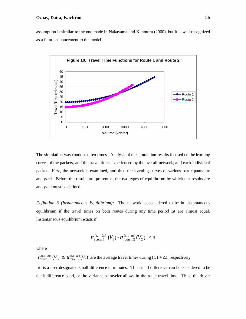
The volume-travel time relationship depicted by the travel time function for both routes can be seen

in Figure 10. Route 1 is a longer path and has more capacity. Hence, the travel time curve for this

route is flatter, and has a smaller slope. Route 2 is a shorter, and quicker route, with a smaller

capacity. Hence, the function is steeper and has a larger slope. Solving the travel time functions

for equilibrium conditions yields a flow of 2800 vehicles per hour with a corresponding travel time

of 30 minutes on Route 2, and 29.5 minutes on Route 1. The network used here is the same

network used in Iida et al. for the analysis of route choice behavior (1992).

The output of the simulation lists each customer’s travel times, route selection, volume on both

routes, and route choice probabilities for each day. Output data also includes the total number of

vehicles traveling on each route each day. One important point that needs to be emphasized is the

fact that our model does not incorporate “departure time” choice of travelers. It is assumed that

travelers, packets in this case, depart during the same [t, t + ∆t] time period every morning. This


assumption is similar to the one made in Nakayama and Kitamura (2000), but it is well recognized

as a future enhancement to the model.

Figure 10. Travel Time Functions for Route 1 and Route 2

05

101520253035404550

0 1000 2000 3000 4000 5000

Volume (veh/hr)

Tra

vel T

ime

(min

utes

)

Route 1Route 2

The simulation was conducted ten times. Analysis of the simulation results focused on the learning

curves of the packets, and the travel times experienced by the overall network, and each individual

packet. First, the network is examined, and then the learning curves of various participants are

analyzed. Before the results are presented, the two types of equilibrium by which our results are

analyzed must be defined.

Definition 3 (Instantaneous Equilibrium): The network is considered to be in instantaneous

equilibrium if the travel times on both routes during any time period ∆t are almost equal.

Instantaneous equilibrium exists if

)( - )( 2) ,(

2_1 ) ,(

1_ ε≤∆+∆+ VttVtt tttroute

tttroute

where

)( 1 ) ,(

1_ Vtt tttroute

∆+ & )( 2) ,(

2_ Vtt tttroute

∆+ are the average travel times during [t, t + ∆t] respectively

ε is a user designated small difference in minutes. This small difference can be considered to be

the indifference band, or the variance a traveler allows in the route travel time. Thus, the driver


will not switch to the other route if the travel time difference between the two routes is within [-

3,+3] minutes.

Definition 4 (Global User Equilibrium): Global user equilibrium is defined as

)( )( 22_11_total

routetotal

route VttVtt =

where

volume1 and volume2 are the total number of cars that used routes 1 and 2 during the overall

simulation period.

The total volumes and corresponding travel times, in minutes, on each route at the end of each

simulation are presented in Table 3. As can be seen, the overall travel times for each route are

very similar. The largest difference is 1.632 minutes, which can be considered negligible. This

fact shows that global user equilibrium, as defined in Definition 4, has been reached.

Table 3. Simulation Results

Route 1 Route 2 Volume Travel Time Volume Travel Time

Global User Equilibrium

3030 31.161 2800 31.877 -0.715 3090 31.616 2800 31.202 0.414 3155 32.118 2800 30.486 1.632 3140 32.001 2800 30.650 1.352 2980 30.789 2800 32.450 -1.660 3095 31.654 2800 31.146 0.508 3000 30.938 2800 32.219 -1.282 3075 31.501 2800 31.369 0.132 3105 31.731 2800 31.035 0.696 3005 30.975 2800 32.162 -1.187

Next, instantaneous equilibrium, described in Definition 3, is examined. Definition 3 ensures that

the difference between route travel times is similar and that each packet is learning the correct

route, namely the shortest route for its departure period. A large difference between route travel

times shows that the network is unstable because one route’s travel time is much larger than that of

the other, and that users are not learning the shortest route for their departure period. Table 4

shows the results of instantaneous equilibrium analysis.


The data is presented in percent form to reflect the 112,800 choices that are made during the

course of the simulation. The percentage of instantaneous equilibrium conditions ranged from

79.333% to 95.500%. This percentage signifies how often instantaneous equilibrium conditions

were satisfied throughout each simulation. For simulation 1, 95% of the 112,800 decisions were

made during instantaneous equilibrium conditions. These results state that most of the packets

choose the shortest route throughout the simulation period.

Figure 11 shows the evolution of instantaneous equilibrium during the course of the simulation.

For the first several days, the values are similar, yet incorrect. This can be attributed to the means

by which the network was loaded. Each packet required several days to begin the learning process.

The slope of each plot represents the learning process. As the packets begin to learn, instantaneous

equilibrium is achieved. Finally, each of these simulations achieved and maintained a high-level of

instantaneous equilibrium for several days before the simulation ended. This fact ensures network

stability and a relationship consistent with Definition 3. If the simulation is conducted for more

than 94 days, it is clear that better convergence results in terms of “instantaneous equilibrium” will

be obtained.

Table 4. Success Rate of Instantaneous Equilibrium

Simulation Number

Instantaneous Equilibrium

1 95.000% 2 86.667% 3 86.000% 4 93.333% 5 79.333% 6 81.667% 7 83.083% 8 90.250% 9 90.333% 10 95.500%


Evolution of Instanteous Equilibrium

00.10.20.30.40.50.60.70.80.9

1

0 20 40 60 80 100

Day

Per

cent

age

Simulation #3Simulation #8Simulation #10

Figure 11. Evolution of Instantaneous Equilibrium

Finally, the learning curves for several packets individual packets can be seen in Figure 12. All of

the curves packets exhibit a high degree of learning. The slope of each curve is steep, which

evidences a quick learning rate. The packets in this figure were chosen randomly. The flat portion

of three of the curves indicates that learning is not yet taking place; rather, instability exists within

the network at that time. However, once stability increases, the learning rate increases greatly.

Another proof that learning is taking place is the percent of correct decisions taken by each packet.

For the packets shown in Figure 12, the percentage of correct decisions were mixed. Packet 658

choose correctly 78% of the time it had to make a route choice decision, while packets 1120

(simulation 4) and 320 choose correctly 73% and 75% of the times these packets had to make route

choice decisions. Obviously, the correct choice is the shortest route. These learning percentages

reflect all 94 days of the simulation. As can be seen from the graph, each packet is consistently

learning throughout the entire simulation. The variability in the plots is due to the randomness

introduced by the generated random number. On any day of the simulation, the random number

generated can cause travelers to choose incorrectly, even though the traveler’s route choice

probability (p1 and p2) favors a certain route (i.e. p1 > p2 or p2 > p1).


Learning Curves for Arbitrary Packets

00.10.20.30.40.50.60.70.80.9

1

0 20 40 60 80 100

Day

Per

cent

age Packet 658 Simulation8

Packet 1120 Simulation 4Packet 1120 Simulation 3Packet 320 Simulation 9

Figure 12. Learning Curves for Arbitrary Packets

Further proof of the accuracy of the SLA-RC model is gained through comparison of Figures 11

and 12. Figure 11 displays the occurrence of instantaneous network equilibrium, whereas Figure

12 displays the learning curve for various travelers. Based on Figure 11, the occurrence of

instantaneous equilibrium is constantly increasing throughout the entire simulation. As

instantaneous equilibrium increases, so does the learning rate of each packet, as seen in Figure 12.

8.0 LEARNING BASED ON THE EXPECTED AND EXPERIENCED TRAVEL

TIMES ON ONE ROUTE

The penalty-reward criterion used in the previous section has been modified to test the learning

behavior of drivers who do not have full information about the network-wide travel time

conditions. This criterion can be described as follows.

If, i router

i act,r

i exp, tt tt ε≤−

Then, the actionα l is considered a success. Otherwise, it is considered a failure and the

probability of choosing route i is reduced according to the linear reward-penalty learning scheme

described in the previous sections.

where


ri exp,tt is the travel time expected by user i on route r.

ri

rflow-free

ri exp, tt tt Ε+=

i routeε = allowed time for early or late arrival

ri act,tt = travel time actually experienced by user i on route r

riΕ is the random error term representing the personal bias of user i and is obtained from a

normal distribution with mean µ = 0, and standard deviation σi, N(µ, σi).

This simulation was conducted for six trials. The expected travel time for each traveler was the

free-flow travel time for each route (same as before) plus a random error generated from the

distribution N(8.5,1.5) minutes. Using these criteria, the following results were obtained.

The range in travel times obtained for each route is shown in Table 5. Travel times on Route 1

ranged from 30.938 minutes to 31.846 minutes, whereas for Route 2, travel times ranged from

30.869 minutes to 32.219 minutes. The difference between overall route travel times ranged from

1.282 minutes to 0.320 minutes, which are relatively small differences in travel time. These results

are similar to the results obtained in the previous simulation. It can be stated that “global user

equilibrium”, as defined in Definition 4, has been achieved.

Route 1 Route 2

Volume Travel Time Volume Travel Time

Global User Equilibrium

3120 31.846 2880 30.869 0.977 3010 31.012 2990 32.105 -1.093 3085 31.578 2915 31.257 0.320 3050 31.312 2950 31.650 -0.338 3050 31.312 2950 31.650 -0.338 3105 31.731 2895 31.035 0.696 3020 31.086 2980 31.991 -0.904 3000 30.938 3000 32.219 -1.282 3010 31.012 2990 32.105 -1.093

Table 5. Travel Time Differences

Table 6 displays the results for instantaneous equilibrium calculations. For this model,

instantaneous equilibrium rates were not as consistent, or high, as in the previous model.


Table 6. Success Rate of Instantaneous Equilibrium

Simulation Number Instantaneous Equilibrium

1 85.167% 2 80.417% 3 88.750% 4 95.750% 5 81.833% 6 88.750% 7 91.000% 8 95.417% 9 80.917% 10 88.833%

The expected travel time for each customer was random, so that some customers could have

smaller expected travel times that were closer to the free-flow travel time, rather than the

equilibrium travel time. On other hand, those customers with larger expected travel times were

closer to equilibrium travel times. Hence, global user equilibrium was achieved when both types of

customers found the shortest route for themselves, since global user equilibrium uses the total

volume on each route. However, instantaneous equilibrium was not always achieved because the

customers with larger expected travel times could travel on the longer route because the difference

between the actual travel time and the expected travel time was still below the minimum. This fact

is consistent with the real behavior of drivers. Some drivers choose longer routes because their

expected arrival times are quite larger than for other drivers.

Finally, the learning rate of individual packets needs to be addressed. Figure 13 shows the learning

rate for four packets. Three of the four packets have a consistent learning rate, and then on day

50, the slope of their learning rate begins to increase dramatically. Packet 340 experienced a high

rate of learning in the beginning of the simulation, which then tapered off slightly. However, by the

end of the simulation, this packet’s learning rate was relatively equal to the learning rates of the

other packets. These four packets choose the correct route approximately 85% of the time they

had to make route choice decisions. The random error term for each packet ranged from 7.05 to

8.45 minutes. These results show that each packet learned the shortest route for their expected

travel times quickly and efficiently.


Figure 12. Learning Curve for Arbitrary Packets

00.10.20.30.40.50.60.70.80.9

1

0 20 40 60 80 100

Day

Per

cent

age Packet 340 Simulation 4

Packet 1100 Simualtion 2Packet 450 Simulation 3Packet 765 Simulation 8

Figure 13. Learning Curves for Arbitrary Packets

9.0 CONCLUSIONS AND RECOMMENDATIONS

In this study, the concept of Stochastic Learning Automata was introduced and applied to the

modeling of the day-to-day learning behavior of drivers within the context of route choice behavior.

A Linear Reward-Penalty scheme was proposed to represent the day-to-day learning process. In

order to calibrate the SLA model, the Internet based Route Choice Simulator (IRCS) was

developed. Data collected from these experiments was analyzed to show that the participants’

learning process can be modeled as a stochastic process that conforms to the Linear Reward-

Penalty Scheme within the Stochastic Automata theory. The model was calibrated using

experimental data obtained from a set of subjects who participated in the experiments conducted at

Rutgers University. Next, a two-route simulation network was developed, and the developed SLA-

RC model was employed to determine the effects of learning on the equilibrium of the network.

Two different sets of penalty-reward criteria were used. The results of this simulation indicate that

network equilibrium was reached, in terms of overall travel time for the two routes, as defined in

Definition 4, and instantaneous equilibrium for each packet, as defined in Definition 3. In the

future, we propose to extend this methodology to include departure time choice and multiple origin-

destination networks with multiple decision points.


REFERENCES

1. Atkinson, R.C., G.H. Bower and E.J. Crothers, An Introduction to Mathematical Learning

Theory, Wiley, New York, 1965.

2. Baba, New Topics in Learning Automata Theory and Applications, Lecture Notes in Control

and Information Sciences, Springer-Verlag, Berlin, 1984.

3. Bush, R.R., and F. Mosteller, Stochastic Models for Learning, Wiley, New York, 1958.

4. Cascetta, E., and Canteralla, G.E., “Dynamic Processes and Equilibrium in Transportation

Networks: Towards a Unifying Theory”, Transportation Science, Vol.29, No.4, pp.305-328,

1985.

5. Cascetta, E., and Canteralla, G.E., “A day-to-day and within-day Dynamic Stochastic

Assignment Model”, Transportation Research, 25a(5), 277-291 (1991).

6. Cascetta, E., and Canteralla, G.E., “Modeling Dynamics in Transportation Networks”, Journal

of Simulation and Practice and Theory 1, 65-91 (1993).

7. Chandrasekharan, B., and D.W.C. Shen, “On Expediency and Convergence in Variable

Structure Stochastic Automata,” IEEE Trans. on Syst. Sci. and Cyber., 1968, Vol.5, pp.145-

149.

8. Davis, N. and Nihan, “Large Population Approximations of a General Stochastic Traffic

Assignment Model” Operations Research (1993).

9. Fu, K.S., “Stochastic Automata as Models of Learning Systems,” in Computer and

Information Sciences II, J.T. Lou, Editor, Academic, New York, 1967.

10. Gilbert, V., J. Thibault, and K. Najim, “Learning Automata for Control and Optimization of a

Continuous Stirred Tank Fermenter,” IFAC Symp. on Adap. Syst. in Ctrl. and Sig. Proc.,

1992.

11. Iida, Yasunori, Takamasa Akiyama, and Takashi Uchida, “Experimental Analysis of Dynamic

Route Choice Behavior,” Transportation Research Part B, 1992, Vol 26B, No. 1, pp 17-32.

12. Jha, Mithilesh, Samer Madanat, and Srinivas Peeta, “Perception Updating and Day-to-day

Travel Choice Dynamics in Traffic Networks with Information Provision,”.

13. Kushner, H.J., M.A.L. Thathachar, and S. Lakshmivarahan, “Two-state Automaton a

Counterexample,” Dec. 1979, IEEE Trans. on Syst., Man and Cyber.s, 1972, Vol. 2, pp.292-

294.


14. Mahmassani, Hani S., and Gang-Len Ghang, “Dynamic Aspects of Departure-Time Choice

Behavior Commuting System: Theoretical Framework and Experimental Analysis,”

Transportation Research Record, Vol. 1037.

15. Najim, K., “Modeling and Self-adjusting Control of an Absorption Column,” International

Journal of Adaptive Control and Signal Processing, 1991, Vol. 5, pp. 335-345.

16. Najim, K., and A. S. Poznyak, “Multimodal Searching Technique Based on Learning

Automata with Continuous Input and Changing Number of Actions,” IEEE Trans. on Syst.,

Man and Cyber., Part B, 1996, Vol. 26, No. 4, pp.666-673.

17. Najim, K., and A.S. Poznyak, eds., Learning Automata: theory and applications, Elsevier

Science Ltd, Oxford, U.K., 1994.

18. Nakayama, Shoichiro and Ryuichi Kitamura, “A Route Choice Model with Inductive

Learning,” Submitted for publication in Transportation Research Board.

19. Narendra, K.S., and M.A.L. Thathachar, Learning Automata, Prentice Hall, New Jersey,

1989.

20. Narendra, K.S., “Learning Automata”, IEEE Transactions on Systems, Man, Cybernetics,

pp.323-333, July, 1974.

21. Rajaraman, K., and P .S. Sastry, “Finite Time Analysis of the Pursuit Algorithm for Learning

Automata,” IEEE Trans. on Syst., Man and Cyber., Part B, 1996, Vol. 26, No. 4, pp.590-

598.

22. Sheffi,Y., “Urban Transportation Networks”, Prentice Hall, 1985.

23. Tsetlin, M.L., Automaton Theory and Modeling of Biological Systems, Academic, NY, 1973.

24. Ünsal, C., John S. Bay, and P. Kachroo, “On the Convergence of Linear REpowerd-Penalty

Reinforcement Scheme for Stochastic Learning Automata,” submitted to IEEE Trans. in Syst.,

Man, and Cyber., Part B, August 1996.

25. Ünsal, C., P. Kachroo, and John S. Bay, “Multiple Stochastic Learning Automata for Vehicle

Path Control in an Automated Highway System,” submitted to IEEE Trans,. in Syst., Man,

and Cyber., Part B, May 1996.

26. Unsal, C., John S. Bay, and Pushkin Kachroo, “Intelligent Control of Vehicles:

Preliminary Results on the Application of Learning Automata Techniques to Automated

Highway System”, 1995 IEEE International Conference on Tools with Artificial

Intelligence.


27. Unsal, C., Pushkin Kachroo, and John S. Bay , “Simulation Study of Multiple Intelligent

Vehicle Control Using Stochastic Learning Automata”, (to be published) Transactions of

the International Society of Computer Simulation, 1997.

28. Vaughn, K.M., Kitamura, K., Jovanis, P., “Modeling Route Choice under ATIS in a

Multinomial Choice Frameworm”, Transportation research Board, 75th Annual Meeting,

Washington D.C., 1996.

Modeling Route Choice Behavior Using Stochastic Learning Automata

Documents

Transcript of Modeling Route Choice Behavior Using Stochastic Learning Automata