MODELING REALISTIC DEGRADATIONS IN NON-BLIND DECONVOLUTION

Jérémy Anger†, Mauricio Delbracio§, and Gabriele Facciolo†

†CMLA, ENS Cachan, CNRS, Université Paris-Saclay, 94235 Cachan, France§IIE, Universidad de la República, Uruguay

ABSTRACT

Most image deblurring methods assume an over-simplisticimage formation model and as a result are sensitive to morerealistic image degradations. We propose a novel variationalframework, that explicitly handles pixel saturation, noise,quantization, as well as non-linear camera response func-tion due to e.g., gamma correction. We show that accuratelymodeling a more realistic image acquisition pipeline leadsto significant improvements, both in terms of image qualityand PSNR. Furthermore, we show that incorporating the non-linear response in both the data and the regularization termsof the proposed energy leads to a more detailed restorationthan a naive inversion of the non-linear curve. The minimiza-tion of the proposed energy is performed using stochasticoptimization. A dataset consisting of realistically degradedimages is created in order to evaluate the method.

Index Terms— Non-blind deconvolution, image deblur-ring, saturation, quantization, gamma correction

1. INTRODUCTION

One of the major sources of image blur is due to camera mo-tion during the sensor integration time. This phenomenon ismost visible in low light conditions, when the integration timehas to be long enough to capture a minimum amount of pho-tons. In this situation, any strong light source present in thescene will certainly lead to pixel saturation, since the dynamicrange to capture will be too large for the sensor.

Most motion deblurring strategies consist in estimating ablur kernel (which represents the effect of the camera motionin the image plane), and then deconvolving the blurred imagewith the estimated kernel. In this paper, we propose a non-blind deconvolution algorithm, which assumes that the kernelis known. The simplest image acquisition model is

v = u ∗ k + n, (1)

We thank Jean-Michel Morel for fruitful comments and discussions.Work partly financed by Agencia Nacional de Investigación e Innovación(ANII, Uruguay) grant FCE_1_2017_135458; Office of Naval research grantN00014-17-1-2552, Programme ECOS Sud – UdelaR - Paris DescartesU17E04, DGA Astrid project « filmer la Terre » n◦ANR-17-ASTR-0013-01,MENRT; DGA PhD scholarship jointly supported with FMJH.

18.41dB

(a) Degraded image.

25.56dB

(b) Dγinv-TV.

28.60dB

(c) Dfull-TVγ .

Fig. 1: Image deconvolution can be significantly improvedby defining a data fitting term that considers the whole imagepipeline (quantization, noise, saturation, gamma correction)as shown in (c). Details best seen in the electronic version.

where u represents the sharp noiseless ideal image, ∗ denotesthe convolution operator, k is a known blurring kernel whichwe assume stationary, v is the observed blurry image, and nis a realization of white Gaussian or Poisson noise, depend-ing on the formulation. The inverse problem defined in (1)is linear, but significantly ill-posed. There is a huge amountof work seeking to restore images under this formulation [1].Most methods are casted as minimizations of an energy of theform

E(u) = D(u; v) + λR(u), (2)

where D(u; v) (denoted D(u) from now on) is a data fittingterm that enforces the image formation model (1) and R(u)is a regularizer that imposes prior knowledge on the solution.The total variation penalization [2] is often used:

R(u) = TV(u) =

∫|∇u(x)|dx. (3)

Although interesting, the model (1) is over-simplistic. Inmore realistic scenarios due to the physical image acquisi-tion and the complex processing pipeline, non invertible non-linear degradations, such as, quantization and compression,can occur. Under these circumstances, a more accurate for-ward model is needed:

v = Qq(Sc(u ∗ k + n)1γ ), (4)

where Sc(u) = min(c, u) is the pixel saturation operator,Qq(u) = q · round(uq ) is the pixel quantization of step q andγ is a gamma correction coefficient, generally introduced bythe camera manufacturer (usually q= 1

256 , as u(x)∈ [0, 1]).

To avoid modeling the effects of the non-linear processingon the noise, as done by White et al. [3], we approximate theforward model (4) by

v = Qq(Sc(u ∗ k)1γ ) + n, (5)

where n is assumed white and Gaussian. While this is an ap-proximation, the effect of the gamma correction on shot noise(which follows a Poisson distribution) can be assimilated to avariance-stabilizing transform [4].

Due to model mismatch, traditional approaches, that as-sume the simple linear model (1), need to impose a strongimage prior to overcome these degradations. In this work,we propose to adapt the data fitting term to explicitly accountfor these typical degradations. This yields better results as isillustrated in Fig. 1, where a naive restoration model (1) us-ing total variation regularization is compared to the proposedmodel (5) with a gamma corrected TV regularization.

The paper is organized as follows. In Section 2 we re-view state-of-the-art methods that consider realistic acquisi-tion models. In section 3 we present a deconvolution methodthat works under real practical degradations, such as satura-tion or quantization, while considering gamma correction in arigorous way. Finally, in Section 4 we demonstrate the effec-tiveness of our approach on a new dataset of degraded imagesand conclude in Section 5.

2. RELATED WORK

Although image deconvolution has received significant atten-tion in the past decades [5], there are only few works thataddress the deconvolution problem under a realistic imagepipeline (saturated pixels, quantization, gamma correction).

Cho et al. [6] proposed a robust method that explicitlymodel outliers in the degradation process. However, thismethod is only effective when outliers are sparse in well-localized areas (e.g., saturated regions). Gregson et al. [7]proposed a variational stochastic deconvolution framework,inspired on stochastic tomography reconstruction [8], thatworks with different image priors. The method can handlesaturation by discarding saturated pixels and uses a priorin non-linear space. The method is later extended to blinddeconvolution [9], where a two step reconstruction that im-proved the saturation handling is introduced. The first stepreconstructs the latent image by discarding unreliable blurredpixels, and the second one works on the regions that weremasked out in the first phase. Our method is simpler and doesnot need to distinguish reliable from unreliable pixels.

Whyte et al. [3] claim that while saturation can be handledby discarding saturated pixels, a better solution is obtained bymodifying the data term to handle saturation explicitly. Thesaturation operator (clipping) is approximated with a smoothfunction allowing to compute its derivative. In this work, wepresent a similar approach, but it does not require to approx-imate the non-smooth saturation operator. The authors also

proposed a split update between reliable and unreliable pix-els. Although it effectively reduces ringing, it introduces bluras we show in the experimental section.

Camera response functions, including the gamma curve,are typically invertible functions. As such, some methods [6]directly invert the non-linear curve before deconvolving theimage. However, if the image was quantized in the non-linearspace, inverting the response curve results in non uniformquantization in the linear pixel space.

3. METHOD

In this section, we present different formulations that incor-porate data fitting terms to handle the following degradations:saturation, quantization, and gamma correction. Each prob-lem is formulated as an energy of the form (2), that is min-imized using the Stochastic Deconvolution framework [10].This framework is based on a coordinate descent algorithmwith a Metropolis-Hastings strategy guiding the pixel sam-pling. The method is derivative-free and can be applied toany energy minimization problem, although its convergenceis not guaranteed for non-smooth functions.

At each step of Stochastic Deconvolution, a pixel is drawneither by selecting a pixel nearby the previous sampled one orby randomly choosing a new position. Given a pixel position,the method evaluates the difference of energy that a small in-crease or decrease of the given pixel value would produce. Ifthe energy decreases, the new value is kept and the algorithmis more likely to chose a nearby pixel in the next iteration.Since this process affects a single pixel of the solution at atime, the energy change due to the data and regularizationterms can be computed by evaluating a small number of pix-els surrounding the sampled one [10]. Convolution bound-aries are handled by padding the image and considering thedata fitting term only on valid pixels. In what follows, unlessotherwise specified, we use a total variation penalization (3).

Saturation. Pixel saturation occurs when the scene dynamicrange is larger than the one captured by the camera sensor. Inthis case, high intensities are clipped to the maximum sensorcapacity, resulting in information loss. The saturation modelthat we use is very simple, yet leads to competitive results. Ifc is the sensor saturation limit, the considered data term is

DS(u) = ‖min(c, u ∗ k)− v‖2. (6)

Instead of discarding saturated pixels, this formulation ex-presses the fact that the estimated sharp image convolved bythe motion blur kernel has to be saturated in the same pixelsas the observed image, even if the exact intensity values arelost. Note that the data fitting term is equal to zero in the sat-urated pixels that match. This implies that these regions areregularized by the prior, independently of the regularizationstrength (controlled by λ).

This model works well on small saturated regions. Forlarger regions, we observe an over-smoothed restoration andmissing pixel values cannot be properly restored (see Fig. 4e).Quantization. A direct way to handle quantization is to ex-plicitly introduce it as a constrained minimization problem

argminu

R(u) s.t. Q(u ∗ k) = v, (7)

where Q is the quantization operator. Note that this problemconsiders a noiseless observation. The data term in the asso-ciated Lagrangian relaxation is

DQfw(u) = ‖Q(u ∗ k)− v‖2. (8)

Let us denote Equation (8) as the forward quantization en-ergy. This data fitting term is piecewise constant; in general,a small perturbation in u does not introduce any change on theenergy, making the energy difficult to optimize. More impor-tantly, this model does not exploit the nature of the problem:given two different images, u1 and u2 such that Q(u1 ∗ k) =Q(u2 ∗k) 6= v, the data fitting term (8) leads to the same cost,whereas one image could be closer to the true latent sharpone. Hence the cost should favor one over the other.

Thus, we propose to replace the constraint Q(u ∗ k) = vby (u ∗ k)(x) ∈ Q−1(v(x)) where Q−1(s) = [s− q

2 , s+q2 ]

is the quantization error interval centered at s. This yields

argminu

R(u) s.t. (u ∗ k)(x) ∈ Q−1(v(x)), ∀x. (9)

In this formulation, if the estimate is not within the quantiza-tion error, we can compute a distance to the interval, namely

DQcx(u) =

∥∥∥∥(|u ∗ k − v| − q

2

)+

∥∥∥∥2 , (10)

where (·)+ = max(·, 0). Let us denote (10) as the convexifiedquantization energy. With this formulation the penalization iszero when the current residual is within the quantization error,while it is quadratic when the estimated sharp image u is farfrom the solution. Overfitting the observed image further thanthe quantization is thus avoided and model can successfullyrestore the image even with a low regularization weight.Gamma correction. Since images are stored in a non-linearcolor space, through the use of gamma correction, the decon-volution cannot be performed directly. Indeed, if not prop-erly handled, the gamma correction produces ringing aroundstrong edges during deconvolution [11].

The usual way to deal with gamma correction is to ap-ply the inverse function directly on the observed image [6],leading to

Dγinv(u) = ‖u ∗ k − vγ‖2. (11)

In this case, the model is fitted in linear space.In this work, we argue that the data fitting should be com-

puted directly in the non-linear color space,

Dγ(u) = ‖(u ∗ k)1γ − v‖2, (12)

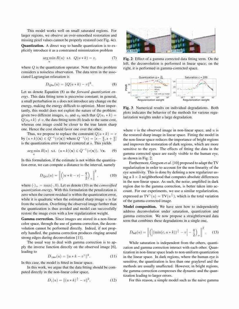
29.19dB 31.54dB

Fig. 2: Effect of a gamma corrected data fitting term. On theleft, the deconvolution is performed in linear space; on theright, it is performed in gamma-corrected space.

10 4 10 2 100 102

Regularization weight

10

20

PSN

R

Quantization q= 16256

Almeida

Whyte

S.D.

S.D. with our model

10 4 10 2 100 102

Regularization weight

15

20

25

Saturation c= 200

Fig. 3: Numerical results on individual degradations. Bothplots indicates the behavior of the methods for various regu-larization weights under a large degradation.

where v is the observed image in non-linear space, and u isthe restored sharp image in linear space. Fitting the model inthe non-linear space reduces the importance of bright regionsand improves the restoration of dark regions, which are moresensitive to the eyes. The effects of fitting the data in thegamma corrected space are easily visible to the human eye,as shown in Fig. 2.

Furthermore, Gregson et al. [10] proposed to adapt the TVregularization in order to account for the non-linearity of theeye sensitivity. This is done by defining a new regularizer us-ing a 3 × 3 neighborhood that computes absolute differencesin the non-linear space. As such, the noise, amplified in darkregion due to the gamma correction, is better taken into ac-count. For our experiments, we use a similar regularization,expressed as TVγ(u) = TV(u

1γ ), which is the total variation

of the gamma-corrected image.Model composition. We have seen how to independentlyaddress deconvolution under saturation, quantization andgamma correction. We now propose a straightforward dataterm that combines these degradations in a single one,

Dfull(u) =

∥∥∥∥(∣∣∣(min(c, u ∗ k))1γ − v

∣∣∣− q

2

)+

∥∥∥∥2 . (13)

While saturation is independent from the others, quanti-zation and gamma correction interact with each other. Quan-tization in non-linear space leads to non-uniform quantizationin the linear space. In dark regions, where the human eye issensitive, the quantization is less than one graylevel and themethods are usually unaffected. However, in bright regions,the gamma correction compresses the dynamic and the quan-tization leading to larger errors.

For this reason, a simple model such as the naive gamma

(a) Ground-truth.

17.00dB

(b) Observation.

22.77dB

(c) Almeida [12].

23.54dB

(d) Whyte [3].

26.74dB

(e) DS (6).

Fig. 4: Large saturation results (image clipped at intensity 200). The proposed model present less artifacts than [12] and [13].

inversion (11) that considers the gamma correction invertibleeven though the image is quantized, produces artifacts espe-cially around bright regions. Our model effectively handlesthe interactions between all degradations.

4. EXPERIMENTS

First, we study the effectiveness of the different modelsindividually. Our results are compared to two state-of-the-art methods. We compared our results with the methods ofAlmeida et al. [12] and Whyte et al. [3]. The first one uses theTV prior, which is representative of the literature, and handlesaccurately the boundary conditions. The second one is basedon the Richardson-Lucy deconvolution algorithm [14], whichis more robust to ringing, and in this version, also handlesboundary conditions as well as saturation. Then, we presentqualitative and quantitative results on a synthetic but realisticdataset, and show that modeling the complete degradationpipeline significantly improves the results.

Individual degradations. We evaluate two of our degrada-tion models: saturation and quantization. Gamma correctionis not evaluated individually as it can be directly inverted if noother degradation is present. For each modality, we apply theforward model to images of BSDS300 [15], vary the strengthof the degradation and record the best PSNR obtained by op-timizing the regularization weight. Fig. 3 shows the PSNRobtained by varying the regularization weight for the differ-ent methods under quantization with 16 levels and saturationat intensity 200. We note that, while the PSNR of our methodfor quantization is slightly lower than the others, it is morestable when sweeping the regularization weight. For satura-tion, our model clearly outperforms both [12] and [3], this isconfirmed by the qualitative evaluation shown in Fig. 4.

A realistic model. To assess the gain of our individual mod-els over a traditional model that does not consider the degra-dations, we created a realistic dataset. The dataset was createdfrom eight sharp natural images. The images are converted tolinear space, by applying the inverse gamma curve, and sub-sampled to reduce the residual quantization and noise. Then,each image is synthetically blurred using one of the kernelsof Levin et al. [16], and saturated by clipping the pixels at the98th percentile. Images are converted back to the non-linearcolor space, where additive white Gaussian noise of σ2 = 5is added. Finally a quantization with q = 1

256 is applied.

Almeida Whyte D inv DS, Dfull D inv DS, Dfull

24

26

28

30

PSNR

TV TV

Fig. 5: PSNR statistics for the different models on a realis-tic dataset. DS,γ is a combination of Eq. (6) and Eq. (12).The orange bar indicates the median PSNR and the highestand lowest bar indicates the maximum and minimum PSNRobtained over the eight images.

Fig. 5 shows the PSNR results obtained with three mod-els. From these results, we observe that considering all thedegradations improves the results. Modeling the quantizationdoes not always improve the PSNR but makes the minimiza-tion less sensitive to the regularization weight. We also reportthe results obtained by using the gamma corrected total varia-tion. When combined with our model it yields a large gain inPSNR as well as in image quality (see Fig. 1). Due to spaceconstraints, the dataset and the full resolution results are avail-able on the project webpage: https://goo.gl/oids7H.

5. CONCLUSION

We proposed a non-blind image deconvolution method thathandles non-linear degradations including, saturation, noise,gamma correction, and quantization. The optimization is pos-sible thanks to a relaxed formulation of the quantization dataterm. The minimization of the resulting energy is performedby stochastic deconvolution [10]. Our experiments high-light the importance of modeling these realistic degradationspresent in the image processing pipeline. For the gammacorrection, we show that the usual gamma inversion mightintroduce errors when the image is quantized in a non-linearcolor space, such as sRGB.

As future work, we would like to extend the method toblind image deconvolution, and study if kernel estimation canbenefit from a more accurate image formation model. Wealso plan to explore the incorporation of other regularizationterms, which could further improve the results.

6. REFERENCES

[1] R. Wang and D. Tao, “Recent Progress in Image De-blurring,” ArXiv 1409.6838, pp. 1–53, 2014.

[2] L. I. Rudin, S. Osher, and E. Fatemi, “Nonlinear totalvariation based noise removal algorithm,” Physica D,vol. 60, no. 1-4, pp. 259–268, 1992.

[3] O. Whyte, J. Sivic, and A. Zisserman, “DeblurringShaken and Partially Saturated Images,” InternationalJournal of Computer Vision, vol. 110, no. 2, pp. 185–201, 2014.

[4] F. J. Anscombe, “The transformation of poisson, bino-mial and negative binomial data,” Biometrika, vol. 35,pp. 246–254, 1948.

[5] D. Kundur and D. Hatzinakos, “Blind image deconvo-lution,” IEEE signal processing magazine, vol. 13, no.3, pp. 43–64, 1996.

[6] S. Cho, J. Wang, and S. Lee, “Handling outliers in non-blind image deconvolution,” in Proceedings of the IEEEInternational Conference on Computer Vision, 2011, pp.495–502.

[7] J. Gregson, F. Heide, M. B. Hullin, M. Rouf, andW. Heidrich, “Stochastic Deconvolution,” in 2013 IEEEConference on Computer Vision and Pattern Recogni-tion. jun 2013, pp. 1043–1050, IEEE.

[8] J. Gregson, M. Krimerman, M. B. Hullin, and W. Hei-drich, “Stochastic tomography and its applications in 3dimaging of mixing fluids.,” ACM Trans. Graph., vol. 31,no. 4, pp. 52–1, 2012.

[9] L. Xiao, J. Gregson, F. Heide, and W. Heidrich,“Stochastic Blind Motion Deblurring,” Image Process-ing, IEEE Transactions on, vol. 24, no. 10, pp. 3071–3085, 2015.

[10] J. Gregson, F. Heide, M. B. Hullin, M. Rouf, andW. Heidrich, “Stochastic deconvolution,” in Proceed-ings of the IEEE Computer Society Conference on Com-puter Vision and Pattern Recognition, 2013, pp. 1043–1050.

[11] Y.-W. Tai, X. Chen, S. Kim, S. J. Kim, F. Li, J. Yang,J. Yu, Y. Matsushita, and M. S. Brown, “Nonlinear cam-era response functions and image deblurring: Theoreti-cal analysis and practice,” IEEE transactions on patternanalysis and machine intelligence, vol. 35, no. 10, pp.2498–2512, 2013.

[12] M. S. C. Almeida and M. Figueiredo, “Deconvolvingimages with unknown boundaries using the alternatingdirection method of multipliers,” IEEE Transactions onImage Processing, vol. 22, no. 8, pp. 3074–3086, 2013.

[13] R. L. White, “Image Restoration Using the DampedRichardson-Lucy Method,” The Restoration of HST Im-ages and Spectra II, pp. 104–110, 1994.

[14] W. H. Richardson, “Bayesian-Based Iterative Methodof Image Restoration,” Journal of the Optical Society ofAmerica, vol. 62, no. 1, pp. 55, 1972.

[15] D. Martin, C. Fowlkes, D. Tal, and J. Malik, “A databaseof human segmented natural images and its applicationto evaluating segmentation algorithms and measuringecological statistics,” in Proc. 8th Int’l Conf. ComputerVision, July 2001, vol. 2, pp. 416–423.

[16] A. Levin, Y. Weiss, F. Durand, and W. T. Freeman,“Understanding and evaluating blind deconvolution al-gorithms,” 2009 IEEE Computer Society Conference onComputer Vision and Pattern Recognition Workshops,CVPR Workshops 2009, pp. 1964–1971, 2009.