Modeling population structure under hierarchical

Dirichlet processes

M. De Iorio, L.T. Elliott, S. Favaro∗ , K. Adhikari and Y.W. Teh

Department of Statistical ScienceGower Street

London WC1E 6BTUnited Kingdom

e-mail: m.deiorio@ucl.ac.uk

Department of Economics and StatisticsCorso Unione Sovietica 218/bis

10134 TorinoItaly

e-mail: stefano.favaro@unito.it

Department of Genetics, Evolution and EnvironmentGower Street

London WC1E 6BTUnited Kingdom

e-mail: k.adhikari@ucl.ac.uk

Department of Statistics1 South Parks Road

Oxford OX1 3TGUnited Kingdom

e-mail: elliott@stats.ox.ac.uk e-mail: y.w.teh@stats.ox.ac.uk

Abstract: We propose a Bayesian nonparametric model to infer population admixture, extendingthe Hierarchical Dirichlet Process (HDP, Teh et al. 2006) to allow for correlation between loci due toLinkage Disequilibrium. Given multilocus genotype data from a sample of individuals, the model allowsinferring classifying individuals as unadmixed or admixed, inferring the number of subpopulationsancestral to an admixed population and the population of origin of chromosomal regions. Our modeldoes not assume any specific mutation process and can be applied to most of the commonly used geneticmarkers. We present a MCMC algorithm to perform posterior inference from the model and discussmethods to summarise the MCMC output for the analysis of population admixture. We demonstratethe performance of the proposed model in simulations and in a real application, using genetic datafrom the EDAR gene, which is considered to be ancestry-informative due to well-known variations inallele frequency as well as phenotypic effects across ancestry. The structure analysis of this datasetleads to the identification of a rare haplotype in Europeans.

AMS 2000 subject classifications: Primary ...; Secondary ....Keywords and phrases: Admixture Modelling, Bayesian Nonparametrics, Population startification,SNP data, MCMC algorithm.

1. Introduction

Population stratification, or population structure, refers to the presence of a systematic difference in geneticmarkers’ allele frequencies between subpopulations due to variation in ancestry. This phenomenon arisesfrom the bio-geographical distribution of human populations. The analysis of population structure presentsan important problem in population genetics and arises in many contexts. It is central to the understanding ofhuman migratory history and the genesis of modern populations [49, 47]. The associated admixture analysisof individuals is important in correcting the confounding effects of population ancestry on gene mapping [60]and association studies [42]. It is also useful in the analysis of gene flow in hybridization zones [16] and invasivespecies [46], conservation genetics [59] and domestication events [35]. The establishment of inexpensive singlenucleotide polymorphism (SNP) genotyping platforms in recent years has facilitated collection of markers

∗Also affiliated to Collegio Carlo Alberto, Moncalieri, Italy.

1

arX

iv:1

503.

0827

8v1

[st

at.A

P] 2

8 M

ar 2

015

to assess genetic ancestry in human populations and in general to investigate genetic relationships in livingorganisms. This paper focuses on a particular form of population structure: admixture. Genetic admixturesoccur when two or more previously isolated populations begin interbreeding, resulting in the introduction ofnew genetic lineages into a population (e.g. the African-American population).

Broadly speaking, the aim of population structure analysis based on genetic data are: (i) detection ofpopulation structure; (ii) estimating the number of subpopulations in a sample; (iii) assigning individualin subpopulations; (iv) defining the number of ancestral populations in admixed populations; (v) inferringancestral population proportions to admixed individuals; (vi) identifying the genetic ancestry of distinctchromosomal segments within an individual. A variety of modelling approaches have been proposed in theliterature. Two of the most widely used approaches are Principal Component Analysis (PCA) and model-based estimation of ancestry, mainly involving clustering techniques or hidden Markov models. The PCAapproach has been used to infer population structure for several decades. In the PCA approach, the indi-viduals’ genotypes are projected onto a lower dimensional space so that the locations of individuals in theprojected space reflects their genetic similarities [38, 34]. It should be noted that the top principal com-ponents do not always capture population structure but may reflect family relatedness, long range linkagedisequilibrium or simply genotyping artefacts. Model based methods aim to reconstruct historical events andtherefore to infer explicitly genetic ancestry (e.g. [43, 55, 2]). In the structured association approach samplesare assigned to sub-population clusters, possibly allowing for fractional membership.

An influential early approach is STRUCTURE by Pritchard et al. (2000) [43], which assumes that indi-viduals come from one of K sub-populations. Based on Bayesian mixture models, population membershipand population specific allele frequencies are jointly estimated from the data. This simple framework canbe extended to genetic admixtures, allowing individuals to have ancestry from more than one population.For each individual, STRUCTURE determines what proportion of the individuals’ genome comes from eachpopulation, while the alleles at different loci are modelled conditionally independently given these admixtureproportions. Taking a Bayesian approach to inference, independent priors on the allelic profile parametersof each population are specified and posterior inference is performed through Markov chain Monte Carlo(MCMC). Various extensions to STRUCTURE have been proposed to address a number of shortcomings.

One problem with STRUCTURE, which we address in this paper , is that of admixture linkage disequilib-rium among neighbouring loci. When individuals from different groups admix, their offsprings’ DNA becomea mixture of the DNA from each admixing group. Chunks of DNA are passed along through subsequentgenerations, up to the present day. Therefore, the genomes of the descendants contain segments of DNAinherited from each of the original populations. The shorter the distance between two loci, the higher theprobability that the population of ancestry will be the same at these two loci. This means that ancestry statesare autocorrelated. The lengths of uninterrupted DNA segments inherited from each sub-population reflecthow long ago the admixture event occurred. In general long uninterrupted segments from each populationimply a recent admixture event. The original version of STRUCTURE did not deal with admixture linkagedisequilibrium and as a result it is necessary to thin out tightly-linked loci to reduce correlations which canaffect the quality of inference. In [13], Falush et al. (2003) improved on this issue by introducing a module tomodel linkage locally among neighbouring loci, using a Markov model which segments each chromosome intocontiguous regions with shared genetic ancestry. This allows local genetic ancestry from genotype data to beinferred, as opposed to the global admixture proportions in [43]. Such local ancestry estimation gives morefine-grained information about the admixture process. In [43] and [13], each population is characterised by anallele frequency profile and they assume that the alleles at each locus are independent. Further dependencecan be modelled by introducing dependence among allelic profiles due to common ancestry [13] or by using aMarkov model for the alleles conditionally on the ancestral segmentation [55]. Another class of models useshaplotypic profiles as richer representations for the allelic dependence within populations [21].

Another important statistical concern in admixture modelling, which we address in this paper, is thedetermination of the number of ancestral populations. In Pritchard et al. (2000) [43], this is achieved usinga model selection criteria based on MCMC estimates of the log marginal probabilities of the data and theBayesian deviance information criterion, though it has been noted by [13] that such estimates are highlysensitive to prior specifications regarding the relatedness of populations. See also Corander et al. (2003) [8]and Evanno et al. (2005) [12] for other parametric approaches to determining the number of populations.One way in which such model selection can be sidestepped is by using Bayesian nonparametric models [22],

2

which offer a flexible framework and do not require the specification of a fixed and finite model size (which,in our context, is the number of populations). Rather, one assumes an unbounded potential model size, ofwhich only a finite part is observed on a given finite dataset. Such ideas have been applied to populationstructure inference by Huelsenbeck and Andolfatto [25] who used the Dirichlet Process (DP) to define aBayesian nonparametric counterpart to the “no-admixture” model of Pritchard et al. (2000) [43] (see alsoDawson and Belkhir [9] and Pella and Masuda [39] for extensions to polyploid data), and by Sohn et al.(2012) [53] who used infinite hidden Markov models [6] for modelling linkage disequilibrium in admixturemodelling.

In this paper, we propose a method for modelling population structure that simultaneously gives estimatesof local ancestries, bypasses difficult model selection issues using Bayesian nonparametrics, and is designed tobe computationally more scalable than current Bayesian nonparametric methods. Our approach is based onusing the hierarchical Dirichlet process (HDP) [56] to non-parametrically model the unknown and uncertainnumber of populations without having to perform costly model selection. Unlike [53], we use a simplifiedtransition model in which, during a transition event, the founder identities on either side of the transitionare independent. This transition model requires a linear rather than quadratic (in the number of founders)number of parameters, as well as a forward-backward algorithm which scales linearly in the number of extantpopulations while introducing less auxiliary variables which can slow down convergence.

In Section 2 we introduce our Bayesian nonparametric model, as well as a novel Markov chain MonteCarlo method which allows efficient exact inference using a retrospective slice sampling truncation scheme.Section 3 describes results of simulation studies, and Section 4 describes population structure analyses ofgenotype data from the EDAR gene region. Section 5 closes with a discussion of our findings as well aspotential future work.

2. Method

We assume we have multilocus genotype data from a sample of admixed individuals arising from a numberof populations. For simplicity, we suppose that there are N haploid individuals genotyped at L loci, and wedenote by X = (xil)1≤i≤N,1≤l≤L the observed data, where xil is the allele of individual i at locus l.

2.1. Model specification

Let K be the number of ancestral populations. We denote by Qi = (qik)1≤k≤K the vector of admixtureproportions of individual i, where qik denotes the proportion of the genome of individual i which can betraced to population k. While previous works used a finite value for K, we will take a Bayesian nonparametricapproach and let K →∞, so that there is an unbounded number of potential populations in the model. Toaccount for dependence among loci, we use the model of linkage proposed by Falush et al. (2003) [13]. Thisemploys a hidden Markov model which splits the genome into contiguous chunks with common ancestry. Themodel is parameterised by: dl, the genetic distance between locus l and locus l+ 1, for each l = 1, . . . , L− 1,and r, the rate at which splits occur. Let zil be a variable which denotes the population ancestry at locus lof individual i, and sil be a binary variable which denotes whether locus l and locus l + 1 are in the samechunk (sil = 1) or not (sil = 0). The variables Sil can be thought of as linkage indicators. The transitionmodel is as follows:

zi1 ∼ Discrete(Qi) (2.1)

si,l+1 ∼ Bernoulli(e−rdl), l = 1, . . . , L− 1

zi,l+1|si,l+1, zil

= zil if si,l+1 = 1,

∼ Discrete(Qi) if si,l+1 = 0.

The probability of a split between loci l and l+1 is 1−e−rdl , and the ancestral populations of each chromosomesegment are independent and identically distributed, with probability qik for the ancestral population to bek for each chunk. The admixture model of Prichard et al. (2000) [43] can be recovered as r →∞, as all locibecome independent and the chunks consist of a single locus.

3

The model is completed by specifying the likelihood function for the observed alleles. We will assume thatwithin each population Hardy-Weinberg equilibrium holds, and we can model the the allelic profile of thekth population simply by specifying the vector of allele frequencies, that is θk = (θkla)1≤l≤L,1≤a≤A, whereθkla is the probability for allele a at locus l in population k. That is,

xil|zil = k ∼ Discrete(θkl) (2.2)

where θkl = (θkla)1≤a≤A. For example, in the case of single nucleotide polymorphism (SNP) data, xil arebinary valued and modelled using Bernoulli distributions with means given by θkl1.

2.2. Prior specification and Bayesian nonparametrics

We use a Dirichlet prior for the admixture proportions Qi. The typical prior in previous works [5, 45, 43,13] is given by a symmetric Dirichlet distribution, which assumes that all populations have a priori equalcontribution to the observed genomes. We will use an asymmetric Dirichlet with mean Q0 = (q0k)1≤k≤Kinstead, to capture the assumption that some populations may be more prevalent than others, so has a priorihigher chance of contributing more genetic material to each individual (see also Anderson [3] and Andersonand Thompson [4]):

Qi|Q0 ∼ Dirichlet(αQ0) (2.3)

where α > 0 is a parameter which controls the concentration of the Dirichlet prior around its mean Q0.The asymmetric Dirichlet also allows for a Bayesian nonparametric model, in which the number of popu-

lations K is taken to be infinite, while the corresponding infinite K limit does not lead to a mathematicallywell-defined model for the symmetric Dirichlet. Specifically, consider a hierarchical prior on Q0 expressed asthe so-called stick-breaking representation [52],

For j = 1, 2, . . .: v0j ∼ Beta(1, α0), (2.4)

q0j = v0j

j−1∏j′=1

(1− v0j′)

where α0 is a hyperparameter which controls the overall diversity of populations, with larger α0 correspondingto a larger number of populations with more uniform proportions. The conditional distribution of Qi givenQ0 is still a Dirichlet as given in (2.3), though we need to extend the definition to one for infinite-dimensionalvectors. Specifically, a constructive definition of such an infinite-dimensional Dirichlet is given as follows:

For j = 1, 2, . . .: vij ∼ Beta(αv0j , α(1−j∑

j′=1

v0j′)) (2.5)

qij = vij

j−1∏j′=1

(1− vij′).

While our model assumes theoretically the existence of an infinite number of populations, given a particularfinite-sized dataset, only a finite (but random) number of populations will be used to model the data, andthe posterior distribution over this number can be used to estimate the number of populations exhibited inthe data; see Subsection 2.4.1 for details.

The model is completed by specifying a prior on α, α0, r and θkl, k = 1, . . . ,K; l = 1, . . . , L. For eachpopulation k, we use independent Dirichlet for the allele frequencies at each locus. In the case of SNP data,this implies assuming independent Beta prior for each locus in each subpopulation. In our simulations andour application to the EDAR data, we take θkl1 ∼ Beta(cµl, c(1−µl)), where ml denotes the prior mean forthe allele frequency, assumed to be the same for all ancestral populations and c is a concentration parameter.We choose independent Gamma priors for α and α0 for computational reasons. We specify a uniform prior

4

on log r, on a fairly large interval. Recall that dl denotes the genetic distance between adjacent markers. Ifit is measured in morgans, then r can be interpreted as an estimate of t, the number of generations sincethe admixture event [13]. When the genetic distance between loci is not available, we can use as a proxy thephysical distance measured in nucleotides. In this case r be interpreted as an estimate of the product of tand the recombination rate (expected number of crossovers per base pair per meiosis).

Another important issue which arises is the computational requirements for inference in a model with aninfinite number of populations. In this regard, a range of recent truncation and marginalisation techniquescan be applied allowing for exact inference using finite computational resources [32, 58, 37, 14]. We proposea particular approach in Subsection 2.4, after discussing in the next subsection the theoretical motivationfor the hierarchical Dirichlet prior described in (2.3) and (2.4).

2.3. Hierarchical Dirichlet processes

The stick-breaking prior for the overall population prevalences (2.4) imposes a particular ordering on thepopulations, in which populations with higher index have a priori lower prevalences. This is undesirable froma modelling perspective as the induced ordering is artificial, while from a computational perspective it is alsoundesirable as it introduces a label switching problem into the inference, which can slow down convergence ofinference algorithms [26, 37]. In this section we address this issue by developing a more abstract formalism forthe model based on a construction of coupled random probability measures called the hierarchical Dirichletprocess [56] (see also Teh and Jordan [57] for a more recent review).

Let (Θ,Ω) be a measurable space. The Dirichlet process G0 ∼ DP(α0, H) is a random probability mea-sure over (Θ,Ω) with the property that for any measurable partition (A1, . . . , AL) of Θ the random prob-ability vector (G0(A1), . . . , G0(AL)) is distributed according to a Dirichlet distribution with parameters(α0H(A1), . . . , α0H(AL)) [15]. The parameters of the process consist of a positive concentration parameterα0 and a base probability measure H over (Θ,Ω). A variety of more constructive representations exist forthe Dirichlet process, and the reader is referred to Ghoshal [19] for a review on the DP and to Lijoi andPrunster [29] for a review of nonparametric prior distributions generalizing the DP.

One of the noteworthy properties of the Dirichlet process is that the random probability measure G0 isdiscrete almost surely, and can be written in the form

G0 =

∞∑k=1

q0kδθk . (2.6)

The atoms (θk)k≥1 are independent and identically distributed according to the base probability measureH, while the atom masses are independent of the atoms, and have distribution given by the stick-breakingrepresentation (2.4) [52].

In the context of admixture modelling, we will suppose that each atom in G0 corresponds to a populationwith allelic frequencies parameterised by the atom, while the masses correspond to the population proportionsor prevalences. In other words, θk denotes the vector of the population specific allele frequencies for theL loci under investigation. As each individual has its own population proportions while the collection ofpopulations are shared across individuals, we can model this using the hierarchical Dirichlet process (HDP).For each individual i, let Gi be an individual-specific atomic random probability measure. These measuresare conditionally independent and identically distributed given a common base probability measure G0:

Gi|G0 ∼ DP(α,G0) (2.7)

Since each atom in Gi is drawn from G0, the collection of atoms in Gi is precisely those in G0, while eachGi has its own specific atom masses:

Gi =

∞∑k=1

qikδθk (2.8)

where the masses (qik)k≥1 have distribution as given in (2.5). The HDP allows sharing of the ancestral amongthe indivual distributions as the Gi place atoms at the same discrete locations determined by G0 (see Tehet al. (2006) [56] for details).

5

We refer to the proposed model as HDPStructure. In summary, Gi describes the proportion of the alleleson xi = (xi1, . . . , xiL) coming from each of the populations, as well as the parameters of the populations.We model the sequence xi given Gi as follows: (i) first we place segment boundaries according to an non-homogeneous Poisson process with rate rdl, (ii) then the alleles on each segment are generated by picking apopulation of origin according to Gi, then sampling the alleles according to the population distribution. Wehave expressed the hierarchical prior over the population proportions (2.4), (2.5) as the joint distributionof atom masses in a HDP, while the atoms correspond to the population parameters. Further, while thestick-breaking representation imposes a particular ordering among the atoms, there is no ordering of atomsin the representation as random probability measures themselves. As we will see next, this allows for anefficient Markov chain Monte Carlo algorithm for posterior simulation.

2.4. Markov Chain Monte Carlo

In this section we describe a Markov chain Monte Carlo (MCMC) algorithm for posterior simulation in theHDPStructure model. The MCMC sampling algorithm iterates between updates to the random probabilitymeasures (Gi)0≤i≤N , the latent state sequences (sil, zil)1≤i≤N,1≤l<L, and the model parameters in turn,each update conditional upon all the other variables in the model. Updates to the random probabilitymeasures make use of another representation of the HDP called the Chinese restaurant franchise [56], as wellas a retrospective slice sampling technique which allows for a finite truncation to the random probabilitymeasures while retaining exactness of the procedure. Updates to the latent state sequences make use ofan efficient forward filtering-backward sampling procedure as a Metropolis-Hastings proposal distribution.Finally, updates to model parameters are straightforward one-dimensional Metropolis-Hastings updates.Detailed descriptions of these updates are included in the Appendix. MATLAB software implementing thisMCMC scheme is freely available at http://BigBayes.github.io/HDPStructure.

2.4.1. Updates to random probability measures

Conditioned on the model parameters and latent state sequences, the update to the random probabilitymeasures (Gi)0≤i≤N follow standard results for the hierarchical Dirichlet process [56]. As noted previously,since the data is finite, the number of populations used to model the data is finite as well. Conditionedon the latent state sequences zil, suppose the number of such populations (as a function of the latentstate sequences) is K∗. For simplicity, we may index these populations as 1, . . . ,K∗. The random probabilitymeasures can be expressed as:

G0 =

K∗∑k=1

q0kδθk + w0G′0 Gi =

K∗∑k=1

qikδθk + wiG′i (2.9)

for each i = 1, . . . , N , where wi is the total mass of all other atoms in Gi, which are collected, after normalisingby wi, in a random probability measure G′i.

For each i = 1, . . . , N and k = 1, . . . ,K∗, let nik be the number of DNA segments in sequence i assignedto population k. In the Chinese restaurant franchise representation of the HDP, we introduce a set ofdiscrete auxiliary variables mik, taking value 0 if nik = 0, and values in the range 1, . . . , nik when nik >

0. Define n0k =∑Ni=1mik. Then the conditional distributions of the random probability measures given

(nik,mik)0≤i≤N,1≤k≤K∗ is described by the following [56],

(q01, . . . , q0K∗ , w0)|(nik,mik) ∼ Dirichlet(n01, . . . , n0K∗ , α0) (2.10)

(qi1, . . . , qiK∗ , wi)|(nik,mik), (q01, . . . , q0K∗), w0 ∼ Dirichlet(αq01 + ni1, . . . , αq0K∗ + n0K∗ , αw0)

G′0|(nik,mik) ∼ DP(α0, H) (2.11)

G′i|(nik,mik), G′0 ∼ DP(α,G′0)

where the masses form a hierarchy of finite-dimensional Dirichlet distributions while the random probabilitymeasures are independent of the masses and form a hierarchy of DPs as in the prior.

6

A final point of consideration relates to the fact that the random probability measures G′0, (G′i) have

infinitely many atoms, so not all can be simulated explicitly with finite computational resources. We addressthis using a retrospective slice sampling technique to truncate the random probability measures while retain-ing exactness [58, 37, 20]. For each individual i, we introduce an auxiliary slice variable Ci, with conditionaldistribution given the other variables in the model:

qmini = min

l=1,...,Lqizil (2.12)

Ci|(nik,mik), G0, (Gi) ∼ Uniform[0, qmini ]. (2.13)

The slice variables are sampled just before the latent state sequences (whose updates are described in thenext subsection). Further, conditioned on the slice variables, populations whose mass fall below Ci will havezero probability to be selected when the latent state sequence for individual i is updated. As a consequence,only the (finitely many) atoms with mass above the minimum threshold mini Ci need be simulated. This canbe achieved by simulating G′0 and (G′i) using the hierarchical stick-breaking representation (2.4), (2.5) untilthe left-over mass falls below the threshold.

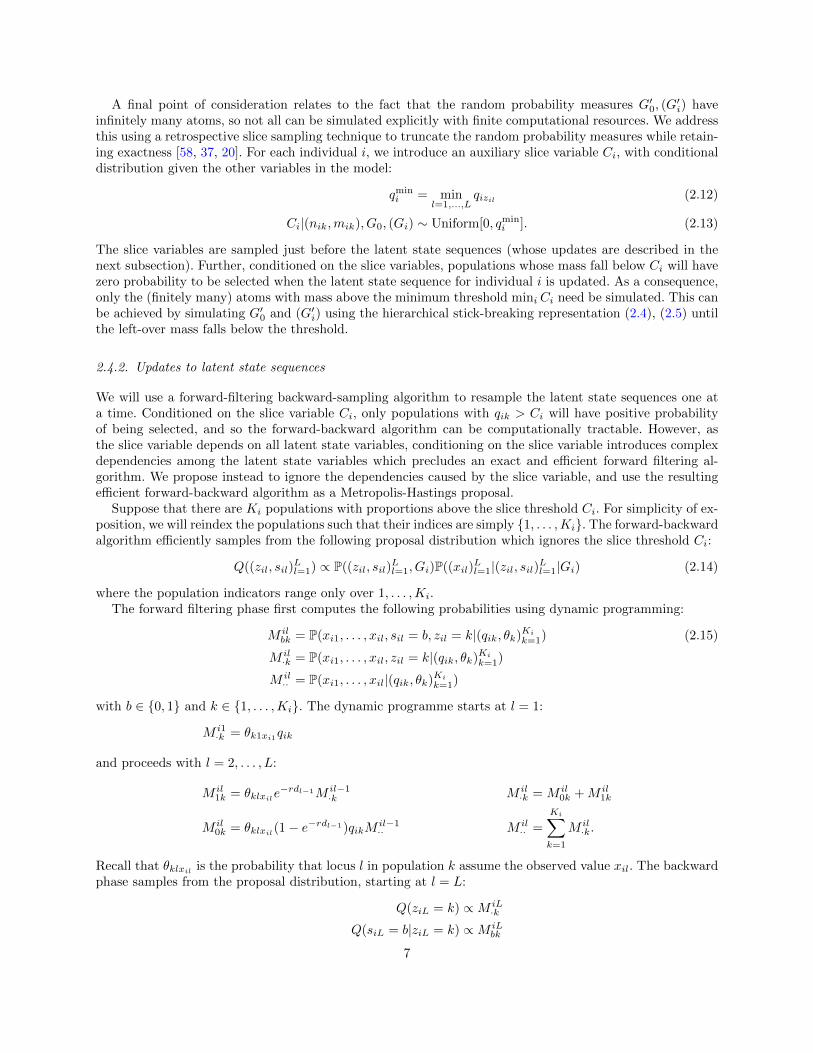
2.4.2. Updates to latent state sequences

We will use a forward-filtering backward-sampling algorithm to resample the latent state sequences one ata time. Conditioned on the slice variable Ci, only populations with qik > Ci will have positive probabilityof being selected, and so the forward-backward algorithm can be computationally tractable. However, asthe slice variable depends on all latent state variables, conditioning on the slice variable introduces complexdependencies among the latent state variables which precludes an exact and efficient forward filtering al-gorithm. We propose instead to ignore the dependencies caused by the slice variable, and use the resultingefficient forward-backward algorithm as a Metropolis-Hastings proposal.

Suppose that there are Ki populations with proportions above the slice threshold Ci. For simplicity of ex-position, we will reindex the populations such that their indices are simply 1, . . . ,Ki. The forward-backwardalgorithm efficiently samples from the following proposal distribution which ignores the slice threshold Ci:

Q((zil, sil)Ll=1) ∝ P((zil, sil)

Ll=1, Gi)P((xil)

Ll=1|(zil, sil)Ll=1|Gi) (2.14)

where the population indicators range only over 1, . . . ,Ki.The forward filtering phase first computes the following probabilities using dynamic programming:

M ilbk = P(xi1, . . . , xil, sil = b, zil = k|(qik, θk)Ki

k=1) (2.15)

M il·k = P(xi1, . . . , xil, zil = k|(qik, θk)Ki

k=1)

M il·· = P(xi1, . . . , xil|(qik, θk)Ki

k=1)

with b ∈ 0, 1 and k ∈ 1, . . . ,Ki. The dynamic programme starts at l = 1:

M i1·k = θk1xi1

qik

and proceeds with l = 2, . . . , L:

M il1k = θklxil

e−rdl−1M il−1·k M il

·k = M il0k +M il

1k

M il0k = θklxil

(1− e−rdl−1)qikMil−1·· M il

·· =

Ki∑k=1

M il·k.

Recall that θklxilis the probability that locus l in population k assume the observed value xil. The backward

phase samples from the proposal distribution, starting at l = L:

Q(ziL = k) ∝M iL·k

Q(siL = b|ziL = k) ∝M iLbk

7

and iterates backwards, for l = L− 1, . . . , 1:

Q(zil = k|sil+1 = 1, zil+1 = k′) ∝ 1(k = k′)

Q(zil = k|sil+1 = 0, zil+1 = k′) ∝M il·k

Q(sil = b|zil = k) ∝M ilbk.

where 1(·) denotes the indicator function and si1 = 0 by construction. In this way we obtain a new samplefor the collection of sil and zil. Finally, the Metropolis-Hastings acceptance probability is a simple expressionwhich accounts for the effect of conditioning on Ci:

min

(1,

qmin-curi

qmin-propi

)(2.16)

where qmin-curi and qmin-prop

i indicate the minimum population proportions (2.12) under the current andproposed states respectively.

The forward-backward algorithm has a computational scaling of O(LKi), linear in both the length ofthe sequence and the number of potential populations, and is the most computationally expensive part ofthe MCMC algorithm. It must be noted that, since the (Gi) are conditionally independent given G0, thealgorithm can be easily parallelised so as to exploit modern parallel computation technology.

2.5. Extensions

The model can be straightforwardly extended to diploid or polyploid data, by assuming that, for eachindividual i, the zi along each of individual i’s chromosomes form independent Markov chains satisfying (2.2).Other extensions of the Bayesian nonparametric admixture model can be introduced to allow correlatedallele frequencies. For instance, following the approaches of Pritchard et al. (2000) [43] and Falush et al.(2003) [13], it is straightforward to introduce a Bayesian nonparametric admixture model with correlatedallele frequencies. Specifically, we can assume that allele frequencies in one population provide informationabout the allele frequencies in another population, i.e. frequencies in the different populations are likelyto be similar (probably due to migration or shared ancestry). This can be achieved by specifying a morecomplex prior structure on θkl., for example employing the correlated allele frequencies model of Falush etal. (2003) [13], which assumes that allele frequencies at locus l in different populations are deviations fromallele frequencies in a hypothetical ancestral population.

At the moment, we use only genetic data to infer admixture parameters. Often it can be useful to includein the model extra information such as physical characteristics (e.g. ethnicity) of sampled individuals or geo-graphic sampling locations [23]. These new sources of information would modify the clustering structure andwould allow the proportion of individuals assigned to a particular cluster to depend on the new information.This would require a specification of a spatiality dependent model on the weights of the random measuresin the HDP.

From a Bayesian parametric perspective, we could also employ other priors such as the Pitman-Yor process[40] and the hierarchical Pitman-Yor process [57]. The Pitman-Yor process is a two-parameter generalizationof the DP, for which a stick-breaking construction and a Chinese restaurant representation still hold. Undercertain assumptions, it can be shown that in the Pitman-Yor process the number of clusters grows muchfaster than for a standard DP and that the cluster sizes decay according to a power law. This property makesthe Pitman-Yor process a more suitable choice in many applications. The implementation of this more flexibleprior would require more expensive computations due to the larger number of extant populations possible.

3. Simulation studies

In order to assess the performance of the model in recovering the number of ancestral populations, weperform simulations based on three demographic scenarios. Each scenario consists of 200 haploid sequences.

8

We consider 60 bi-allelic genetic markers on a 100Kbp segment. Coalescent simulations were performed usingthe software ms [24]. Mutation and recombination rates were set to 2 × 10−8 and 10−8 per base pair pergeneration respectively. The focus is to identify the populations of origin and to infer demographic history.In particular, the main goal is inference on K. The three simulated scenarios we consider are: (i) samplefrom a single random mating population; (ii) admixture model with two parental populations and admixtureproportion of 0.6 and 0.4; (iii) admixture model with three parental populations and admixture proportion0.5, 0.4 and 0.1. Figure 5 shows the posterior distribution of K (after burn-in) under the three scenarios.HDPStructure successfully recovers the number of ancestral populations.

In the simulations we have set the parameters for the Gamma priors on α and α0 as follows: α ∼Gamma(1, 1) and α0 ∼ Gamma(5, 1). Although inference can be sensitive to the choice of the prior onthe number of populations, i.e. to the prior specification on α and α0, we note that as the number ofsequences and/or markers increases the model tends to generate spurious clusters, i.e. clusters with very fewindividuals in them. This is in line with recent results on the clustering properties of the Dirichlet Process[31]. Nevertheless, the number of clusters that covers the majority of the data, i.e. 95-99%, is quite robustto prior specifications (sensitivity analysis results not shown). In general, the biological interpretation of Kis difficult. This is in agreement with the suggestion of Pritchard et al. (2010)[44]:

We may not be able to know the TRUE value of K, but we should aim for the smallest value of K that captures themajor structure in the data.

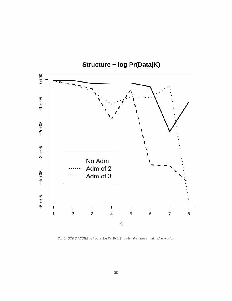
We compare our results with the software STRUCTURE [43, 13, 23], which is arguably the most widelyused software in applications to infer population structure. This software implements the parametric versionof our model, with fixed K (http://pritchardlab.stanford.edu/structure.html). We have run theLinkage model described in Falush et al. (2003) [13], using default settings and assuming independent allelefrequencies between markers. To estimate K, Pritchard et al. (2000) [43] suggested using the value of Kwhich maximises the estimated model log-likelihood, log Pr(Data | K). This latter quantity is estimated bythe MCMC run using an approximation based on the harmonic mean estimator of the Bayesian deviance.For each scenario, we have run STRUCTURE for each value of K, K = 1, . . . , 8. Figure shows the estimatedlog Pr(Data | K) for the three simulated examples. The value K = 1 seems to maximises the model log-likelihood under all scenarios. In general, the authors of the software warn against possible drawback of usingthis criterion and to interpret the results with caution and give suggestions for improvement.

4. Experiments

We demonstrate our model on a dataset of 372 Colombians recently genotyped on the Illumina Human610-Quadv1 B SNP array as part of a genome-wide association study [51]. Latin American samples are uniquelyadvantageous for this purpose [50] because of their well-documented history of extensive mixing betweenNative Americans and people arriving from Europe and Africa. This continental admixture, which hasoccurred for the past 500 years (or about 20-25 generations), gives rise to haplotype blocks which are aboutthe right length for such analysis. Ancient admixture produces very short haplotype fragments which arehard to assign ancestry with certainty, while very recent admixture allows only large haplotype blocks andthere is not sufficient variation in ancestry for individuals.

The Native American population arose as a branch of the East Asian populations who were separatedover 15,000 years ago and consequently isolation and genetic drift shaped their genetic landscape. Thiscaused many SNPs to drift even more than their East Asian counterparts, eventually becoming fixed atthe alternative allele. The Ectodysplasin-A receptor (EDAR) gene, located on chromosome 2, is a commonexample, in particular SNP rs3827760 [30], whose ancestral A allele is 100% prevalent in European andAfrican populations, but the alternative G allele is seen at 94% frequency in Han Chinese and 100% in NativeAmericans. The SNP, a missense mutation, has been observed to have a range of functional effects in humansand replicated in other mammals such as mice, including the characteristic straight hair shape in East Asians[18, 54] and dental morphology [27, 36]. Our dataset does not contain rs3827760, but neighbouring SNPs inLD to rs3827760 are included in the chip panel. This shows a strength of our model does as we manage tocapture the ancestries even in absence of SNP rs3827760, the well-known causal and ancestry-informativeSNP, by making good use of LD information. Figure 5 shows the LD plot for the EDAR region in the

9

Correlation European anc. Amerindian anc. African anc.Cluster 1 (Europe) 0.90 -0.67 -0.36Cluster 2 (America) -0.75 0.92 -0.20Cluster 3 (Africa) -0.36 -0.19 0.76Cluster 4 (New) 0.04 -0.24 0.28

Table 1Correlation between ancestry proportions and cluster occurrence proportion from the Bayesian nonparametric model.

Colombian samples. Overall, EDAR signalling acts during prenatal development to specify the location, sizeand shape of ectodermal appendages, such as hair follicles, teeth and glands [30]. Therefore, we consideredEDAR to be an interesting candidate for admixture analysis as it carries information regarding ancestry dueto its variation across ancestry as well as its range of functional effects, which means it may be showing somesignal of selection.

Genotype information on 372 individuals for 16 SNPs in the EDAR region was available from our Illuminachip data. Genotypes were phased for conversion to haplotype format by ShapeIt2 [10]. Data from a total of828 individuals sampled in putative parental populations were used as reference ancestral groups. These wereselected from HAPMAP, the CEPH-HDGP cell panel [28] and from published Native American data [48] asfollows: 169 Africans (from 5 populations from Sub-Saharan West Africa), 299 Europeans (from 7 West andSouth European populations) and 360 Native Americans (from 47 populations from Mxico Southwards).

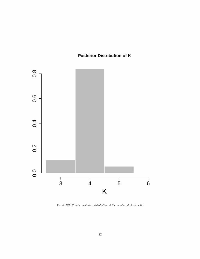
We ran the MCMC sampler for 50,000 iterations. We collected samples after a burn-in of 20,0000 iterationsand thinned every 30 iterations. We specify the following prior distributions for the precision parameters inthe HDP: a0 ∼ Gamma(1, 1), α ∼ Gamma(10, 20). We centre the prior for the mean parameters of the Betabase measure of the HDP around the overall observed allele frequencies, with c = 0.01. The prior for log r isa Uniform on the interval [−500, 5].

The posterior analysis shows evidence of four major ancestral populations in the set of 744 Colombianhaplotypes (see Figure 5). We use the MCMC output to estimate the cluster assignment, i.e. populationallocation, to each of the 4 major ancestral populations for each haplotype sequence and each marker. InFigure 5, we summarise the MCMC output by reporting the clustering that minimizes the posterior expec-tation of Binder’s loss as described by Fritsch and Ickstadt (2009)[17], who also discuss possible alternativessuch as Maximum a posteriori clustering. The four major clusters have admixture coefficients, i.e. relativeproportion of occurrences of each of the clusters, 51.8%, 32.1%, 11.4% and 4.7% respectively. As we haveused a reference panel, we are able to identify in the first cluster, in terms of cardinality, European-originhaplotypes in the sampled Colombians. The second and third clusters correspond to Amerindian and Africanrespectively. This is also confirmed by looking at the “most frequent” haplotype in each cluster. Figure 5shows the raw data assigned to each of the four major ancestral populations. We verify our findings intwo ways. Firstly, we calculate genetic ancestry proportions using reference genotypes as reference ancestralgroups. EDAR-specific ancestry proportions for each of the 372 Colombian samples were estimated usingAdmixture software [2], which provides a faster implementation of the same model in STRUCTURE. Wecorrelated these ancestry proportions to our cluster occurrence proportion (see Table 4). The correlationvalues are very high and support our assignment of ancestry category to the first three clusters. The averageEuropean, Amerindian and African ancestry across Colombian samples are 53.6%, 30.8% and 16.6% respec-tively, which is also very close to our cluster proportions. However, Admixture is a supervised approach andso it cannot give us further details about the fourth, rarer cluster. To explore it further, and also for anotherline of verification, we calculate genetic principal components, in which SNP genotypes for each person isrecoded into 0/1/2 by an additive count of the minor allele on two chromosomes, and this SNP genotypecount matrix is converted to principal components (PC) via the usual method. As European+Amerindiancontinental genetic mixing is the primary source for admixture in our data, the first PC axis reflects this,being positively correlated with European samples and negatively with American samples. The second PCcaptures the other continental component in our samples, namely the African samples. More specifically,PC1 captures the European-Amerindian axis of variation, and PC2 captures the African-European axis. InTable 4 we show correlations of PCs with supervised ancestry values. As further PCs are orthogonal to these,they do not show high correlation with any ancestry component. Consequently, the first PC shows high cor-relations with the first two clusters, and PC2 with the third cluster. As shown in Table 4 the third PC is

10

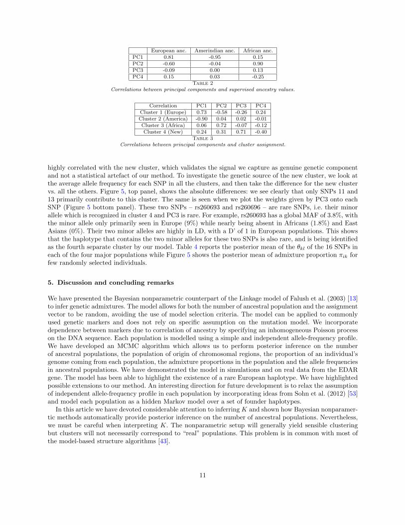
European anc. Amerindian anc. African anc.PC1 0.81 -0.95 0.15PC2 -0.60 -0.04 0.90PC3 -0.09 0.00 0.13PC4 0.15 0.03 -0.25

Table 2Correlations between principal components and supervised ancestry values.

Correlation PC1 PC2 PC3 PC4Cluster 1 (Europe) 0.73 -0.58 -0.26 0.24Cluster 2 (America) -0.90 0.04 0.02 -0.01Cluster 3 (Africa) 0.06 0.72 -0.07 -0.12Cluster 4 (New) 0.24 0.31 0.71 -0.40

Table 3Correlations between principal components and cluster assignment.

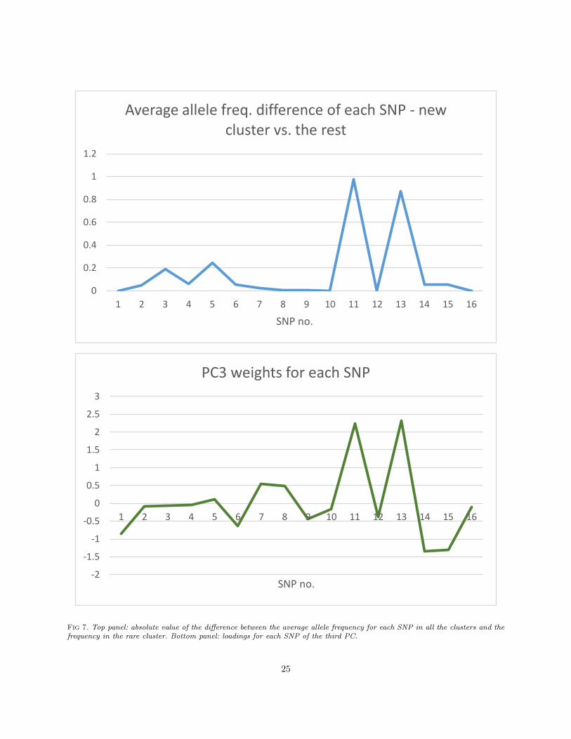
highly correlated with the new cluster, which validates the signal we capture as genuine genetic componentand not a statistical artefact of our method. To investigate the genetic source of the new cluster, we look atthe average allele frequency for each SNP in all the clusters, and then take the difference for the new clustervs. all the others. Figure 5, top panel, shows the absolute differences: we see clearly that only SNPs 11 and13 primarily contribute to this cluster. The same is seen when we plot the weights given by PC3 onto eachSNP (Figure 5 bottom panel). These two SNPs – rs260693 and rs260696 – are rare SNPs, i.e. their minorallele which is recognized in cluster 4 and PC3 is rare. For example, rs260693 has a global MAF of 3.8%, withthe minor allele only primarily seen in Europe (9%) while nearly being absent in Africans (1.8%) and EastAsians (0%). Their two minor alleles are highly in LD, with a D’ of 1 in European populations. This showsthat the haplotype that contains the two minor alleles for these two SNPs is also rare, and is being identifiedas the fourth separate cluster by our model. Table 4 reports the posterior mean of the θkl of the 16 SNPs ineach of the four major populations while Figure 5 shows the posterior mean of admixture proportion πik forfew randomly selected individuals.

5. Discussion and concluding remarks

We have presented the Bayesian nonparametric counterpart of the Linkage model of Falush et al. (2003) [13]to infer genetic admixtures. The model allows for both the number of ancestral population and the assignmentvector to be random, avoiding the use of model selection criteria. The model can be applied to commonlyused genetic markers and does not rely on specific assumption on the mutation model. We incorporatedependence between markers due to correlation of ancestry by specifying an inhomogeneous Poisson processon the DNA sequence. Each population is modelled using a simple and independent allele-frequency profile.We have developed an MCMC algorithm which allows us to perform posterior inference on the numberof ancestral populations, the population of origin of chromosomal regions, the proportion of an individual’sgenome coming from each population, the admixture proportions in the population and the allele frequenciesin ancestral populations. We have demonstrated the model in simulations and on real data from the EDARgene. The model has been able to highlight the existence of a rare European haplotype. We have highlightedpossible extensions to our method. An interesting direction for future development is to relax the assumptionof independent allele-frequency profile in each population by incorporating ideas from Sohn et al. (2012) [53]and model each population as a hidden Markov model over a set of founder haplotypes.

In this article we have devoted considerable attention to inferring K and shown how Bayesian nonparamer-tic methods automatically provide posterior inference on the number of ancestral populations. Nevertheless,we must be careful when interpreting K. The nonparametric setup will generally yield sensible clusteringbut clusters will not necessarily correspond to “real” populations. This problem is in common with most ofthe model-based structure algorithms [43].

11

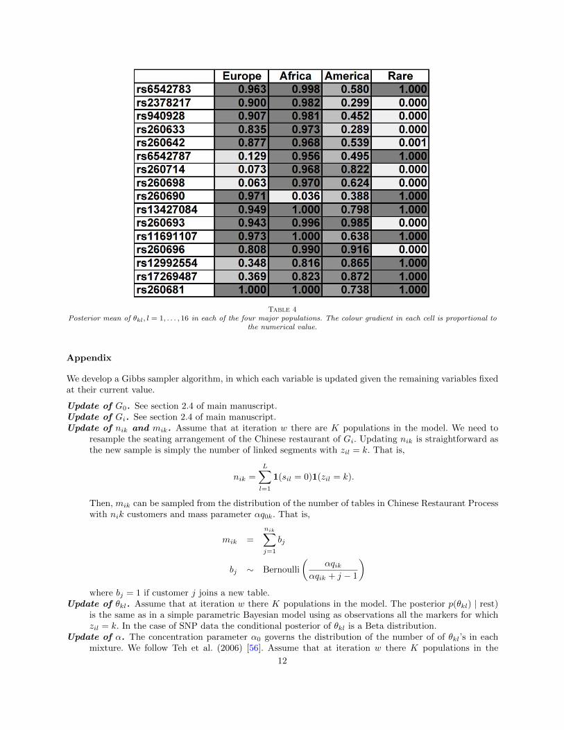
Table 4Posterior mean of θkl, l = 1, . . . , 16 in each of the four major populations. The colour gradient in each cell is proportional to

the numerical value.

Appendix

We develop a Gibbs sampler algorithm, in which each variable is updated given the remaining variables fixedat their current value.

Update of G0. See section 2.4 of main manuscript.Update of Gi. See section 2.4 of main manuscript.Update of nik and mik. Assume that at iteration w there are K populations in the model. We need to

resample the seating arrangement of the Chinese restaurant of Gi. Updating nik is straightforward asthe new sample is simply the number of linked segments with zil = k. That is,

nik =

L∑l=1

1(sil = 0)1(zil = k).

Then, mik can be sampled from the distribution of the number of tables in Chinese Restaurant Processwith nik customers and mass parameter αq0k. That is,

mik =

nik∑j=1

bj

bj ∼ Bernoulli

(αqik

αqik + j − 1

)where bj = 1 if customer j joins a new table.

Update of θkl. Assume that at iteration w there K populations in the model. The posterior p(θkl) | rest)is the same as in a simple parametric Bayesian model using as observations all the markers for whichzil = k. In the case of SNP data the conditional posterior of θkl is a Beta distribution.

Update of α. The concentration parameter α0 governs the distribution of the number of of θkl’s in eachmixture. We follow Teh et al. (2006) [56]. Assume that at iteration w there K populations in the

12

model. Let m.. =∑i,kmik and ni. =

∑k nik. We introduce latent variable wi ∈ [0, 1] and ti ∈ 0, 1,

i = 1, . . . , N , with

wi | α0 ∼ Beta(α0 + 1, ni.)

ti | α0 ∝(

ni.α0 + ni.

)ti.

If α is given a Γ(a, b) hyperprior, then given wi and ti, α has a Gamma distribution with parameters

a+m.. −∑Ni=1 ti and b−

∑Ni=1 logwi.

Update of α0. Given the total number m.. =∑i,kmik of the θkl’s, the concentration parameter α0 governs

the distribution of the number of population K. We use the auxiliary method of Escobar and West [11].If α0 is given a Γ(a, b) hyperprior, it can be resampled by introducing a latent variable γ ∼ Beta(α0 +1,m..) and

p(α0 | K, γ) = πΓ(a+K, b− log(γ)) + (1− π)Γ(a+K − 1, b− log(γ))

where π/(1− π) = (a+K − 1)/m..(b− log(γ)).Update of r. The rate r of the Poisson process is given a Uniform prior on some interval [rL, rU ]. We use a

random walk Metropolis step to update r with proposal distribution centred around the current value.Update of hyperparameters in the base measure H. The proportion of the model involving the hy-

perparameters in H is a convential parametric model. Hence, conditioning on all the other variablesusually leaves us with a standard Bayesian model, often in conjugate form. In the case of SNP data,we have taken θk ∼ H =

∏Ll=1 Beta(cµl, c(1 − µl)). We specify independent Beta(al, bl) for each µl,

l = 1, . . . , L, and update µl using a random walk Metropolis step with proposal distribution centredaround the current value.

References

[1] Aldous, D.J. (1985). Exchangeability and related topics. cole d’t de Probabilits de Saint-Flour, XIII.Lecture notes in Mathematics 1117, Springer, Berlin.

[2] Alexander, D.H., Novembre, J. and Lange K. (2009). Fast model-based estimation of ancestry inunrelated individuals. Genome Research 19, 1655–1664.

[3] Anderson, E.C. (2001). Monte Carlo methods for inference in population genetic models. Ph.D. thesis,University of Washington, Seattle.

[4] Anderson, E.C. and Thompson, E.A. (2002). A model-based method for identifying species hybridsusing multilocus genetic data. Genetics 160, 1217–1229.

[5] Balding, D.J. and Nichols, R.A. (1995). A method for quantifying differentiation between popu-lations at multi-allelic loci and its implications for investigating identity and paternity. Genetica 96, 3–12.

[6] Beal, M.J., Ghahramani, Z. and Rasmussen, C.E. (2002). The Infinite Hidden Markov Model. InNeural Information Processing Systems 14, 577–585, MIT Press, Cambridge, MA.

[7] Blackwell, D. and MacQueen, J. B. (1973). Ferguson distributions via Polya urn schemes. Annalsof Statistics 1, 353–355.

[8] Corander, J., Waldmann, P. and Sillanpaa, M.J. (2003). Bayesian analysis of genetic differenti-ation between populations. Genetics 163, 367–374.

[9] Dawson, K.J. and Belkhir, K. (2001). A Bayesian approach to the identification of panmicticpopulations and the assignment of individuals. Genetics Research 78, 59–77.

13

[10] Delaneau, O., Zagury, J.-F. and Marchini, J. (2013). Improved whole-chromosome phasing fordisease and population genetic studies. Nature Methods 10, 5–6.

[11] Escobar, M.D. and West, M. (1995). Bayesian Density Estimation and Inference Using Mixtures.Journal of the American Statistical Association 90, 577–588.

[12] Evanno, G., Regnaut, S. and Goudet, J. (2005). Detecting the number of clusters of individualsusing the software structure: a simulation study. Molecular Ecology 14, 2611–2620.

[13] Falush, D., Stephens, M. and Pritchard, J.K. (2003). Inference of population structure frommultilocus genotype data: linked loci and correlated allele frequencies. Genetics 164, 1567–1587.

[14] Favaro, S. and Teh, Y.W. (2013). MCMC for Normalized Random Measure Mixture Models.Statistical Science 28, 335–359.

[15] Ferguson, T.S. (1973). A Bayesian analysis of some nonparametric problems. Annals of Statistics 1,209–230.

[16] Field, D.L., Ayre, D.J., Whelan, R.J. and Young, A.G. (2011). Patterns of hybridization andasymmetrical gene flow in hybrid zones of the rare Eucalyptus aggregata and common E. rubida. Heredity106, 841–853.

[17] Fritsch, A. and Ickstadt, K. (2009). Improved Criteria for Clustering Based on the PosteriorSimilarity Matrix. Bayesian Analysis, 4, 367–392.

[18] Fujimoto, A., Kimura, R., Ohashi, J., Omi, K., Yuliwulandari, R., Batubara, L., Mustofa,M.S., Samakkarn, U., Settheetham-Ishida, W., Ishida, T., Morishita, Y., Furusawa, T.,Nakazawa, M., Ohtsuka, R. and Tokunaga, K. (2008). A scan for genetic determinants of humanhair morphology: EDAR is associated with Asian hair thickness. Human Molecular Genetics 17, 835-843.

[19] Ghoshal, S. (2010). Dirichlet process, related priors and posterior asymptotics. In Bayesian Nonpara-metrics, Cambridge University Press, Cambridge.

[20] Jim E. Griffin, J.E. and Walker, S.G. (2013). On adaptive Metropolis-Hastings methods.Statistics and Computing 23, 123–134.

[21] Harris, K. and Nielsen, R. (2013). Inferring demographic history from a spectrum of sharedhaplotype lengths. PLoS Gentics 9, 1–20.

[22] Hjort, N.L., Holmes, C.C., Muller, P. and Walker, S.G. (eds.) (2010). Bayesian nonparamet-rics. Cambridge University Press, Cambridge.

[23] Hubisz, M.J., Falush, D., Stephens, M. and Pritchard, J.K. (2009). Inferring weak populationstructure with the assistance of sample group information. Molecular Ecology Resources 9, 1322–1332.

[24] Hudson, R.R. (2002) Generating samples under a Wright-Fisher neutral model. Bioinformatics 18,337–338.

[25] Huelsenbeck, J.P. and Andolfatto, P. (2007). Inference of population structure under a Dirichletprocess model. Genetics 175, 1787–1802.

[26] Jasra, A., Holmes, C.C. and Stephens, D.A. (2005). Markov Chain Monte Carlo methods andthe label switching problem in Bayesian mixture modeling. Statistical Science 20, 50–67.

14

[27] Kimura, R., Yamaguchi, T., Takeda M., Kondo, O., Toma, T., Haneji, K., Hanihara, T.,Matsukusa, H., Kawamura, S., Maki, K., Osawa, M., Ishida, H. and Oota, H. (2009). Acommon variation in EDAR is a genetic determinant of shovel-shaped incisors. American Journal ofHuman Genetics 85, 528–535.

[28] Li, J.Z., Absher, D.M., Tang, H., Southwick, A.M., Casto, A.M., Ramachandran,S., Cann, H.M., Barsh, G.S., Feldman, M., Cavalli-Sforza, L.L. and Myers, R.M. (2008).Worldwide human relationships inferred from genome-wide patterns of variation. Science 319, 1100–1104.

[29] Lijoi, A. and Prunster, I. (2010). Models beyond the Dirichlet process. In Bayesian Nonparametrics.Cambridge University Press, Cambridge.

[30] Mikkola, M.L. (2009). Molecular aspects of hypohidrotic ectodermal dysplasia. American Journal ofMedical Genetics Part A 149, 2031–2136.

[31] Miller, J.W. and Harrison, M.T. (2014) Inconsistency of Pitman-Yor process mixtures for thenumber of components. Journal of Machine Learning Research 15, 3333–3370.

[32] Neal, R. (2000). Markov chain sampling methods for Dirichlet process mixture models. Journal ofComputational and Graphical Statistics 9, 249–265.

[33] Nicholson, G., Smith, A.V., Jonsson, F., Gustafsson, O., Stefansson, K. and Donelly,P. (2002). Assessing population differentiation and isolation from single-nucleotide polymorphism data.Journal of the Royal Statistical Society Series B 64, 695–715.

[34] Novembre, J. and Stephens, M. Interpreting principal components analyses of spatial populationgenetic variation. Nature Gentics 40, 646–649.

[35] Parker, H.G., Kim, L.V., Sutter, N.B., Carlson, S., Lorentzen, T.D., Malek, T.B.,Johnson, G.S., DeFrance, H.B., Ostrander, E.A. and Kruglya, L. (2004). Genetic structureof the purebred domestic dog. Science 304, 1160–1164.

[36] Park, J.-H., Yamaguchi, T., Watanabe, C., Kawaguchi, A., Haneji, K., Takeda, M., Kim,Y.-I., Tomoyasu, Y., Watanabe, M., Oota, H., Hanihara, T., Ishida, H., Maki, K., Park,S.-B. and Kimura, R. (2012). Effects of an Asian-specific nonsynonymous EDAR variant on multipledental traits. Journal of Human Genetics 57, 508-514.

[37] Papaspiliopoulos, O. and Roberts, G.O. (2008). Retrospective Markov chain Monte Carlomethods for Dirichlet process hierarchical models. Biometrika 95, 169–186.

[38] Patterson, N., Price, A.L. and Reich, D. (2006) Population structure and eigenanalysis. PLoSGenetics 2, 2074–2093.

[39] Pella, J. and Masuda, M. (2006). The Gibbs and split-merge sampler for population mixtureanalysis from genetic data with incomplete baselines. Canadian Journal of Fisheries and AquaticSciences 63, 576–596.

[40] Pitman, J. and Yor, M. (1997). The two-parameter Poisson-Dirichlet distribution derived from astable subordinator. Annals of Probability, 25, 855–900.

[41] Pitman, J. (2006). Combinatorial stochastic processes. Ecole d’Ete de Probabilites de Saint-Flour,XXXII. Lecture Notes in Mathematics 1875, Springer, Berlin.

15

[42] Price, A.L., Zaitlen, N.A., Reich, D. and Patterson, N. (2010). New approaches to populationstratification in genome-wide association studies. Nature Reviews Genetics 11, 459–463.

[43] Pritchard, J.K., Stephens, M. and Donelly, P. (2000). Inference on population structure usingmultilocus genotype data. Genetics 155, 945–959.

[44] Pritchard, J.K., Wen, X. and Falush, D. (2010). Documentation for structure software: Version2.3. Retrieved from http://pritch.bsd.uchicago.edu/structure.html in Summer 2014.

[45] Ranalla, B. and Mountain, J.L. (1997). Detecting immigration by using multilocus genotypes.Proceedings of the National Academy of Sciences 94, 9197–9201.

[46] Ray, A. and Quader, S. (2014). Genetic diversity and population structure of Lantana camara inIndia indicates multiple introductions and gene flow. Plant Biology 16, 651–658.

[47] Reich, D., Thangaraj, K., Patterson, N., Price, A.L. and Singh, L. (2009). ReconstructingIndian population history. Nature 461, 489–494.

[48] Reich, D., Patterson, N., Campbell, D., Tandon, A., Mazieres, S. et al. (2012). Recon-structing Native American population history. Nature 488, 370–374.

[49] Rosenberg, N.A., Pritchard, J.K., Weber, J.L., Cann, H.M., Kidd, K.K., Zhivotovsky,L.A. and Feldman, M.W. (2002). Genetic structure of human populations. Science 298, 2381–2385.

[50] Ruiz-Linares, A., Adhikari, K., Acua-Alonzo, V., Quinto-Sanches, M., Jaramillo, C. etal. (2014) Admixture in Latin America: geographic structure, phenotypic diversity and self-perceptionof ancestry based on 7,342 individuals. PLoS Genetics, 10, 1–13.

[51] Scharf, J.M., Yu, D., Mathews, C.A., Neale, B.M., Stewart, S.E. et al. (2012). Genome-wide association study of Tourette’s syndrome. Molecular Psychiatry 18, 721–728.

[52] Sethuraman, J. (1994). A constructive definition of Dirichlet priors. Statistica Sinica. 4, 639–650.

[53] Sohn, K., Ghahramani, Z. and Xing, E.P. (2012). Robust Estimation of Local Genetic Ancestryin Admixed Populations Using a Non-parametric Bayesian Approach. Genetics 4.

[54] Tan, J., Yang, Y., Tang, K., Sabeti, P. C., Jin, L. and Wang, S. (2013). The adaptive variantEDARV370A is associated with straight hair in East Asians. Human Genetics 132, 1187–1191.

[55] Tang, H., Peng, J., Wang, P. and Risch, N.J. (2005). Estimation of individual admixture:analytical and study design considerations. Genetic Epidemiology 28, 289–301.

[56] Teh, Y.W., Jordan, M.I., Beal, M,J. and Blei, D.M. (2006). Hierarchical Dirichlet processes.Journal of the American Statistical Association 101, 1566–1581.

[57] Teh, Y.W. and Jordan, M.I. (2010). Hierarchical Bayesian nonparametric models with applications.In Bayesian Nonparametrics. Cambridge University Press, Cambridge.

[58] Walker, S.G. (2007). Sampling the Dirichlet mixture model with slices. Communications in Statistics:Simulation and Computation 36, 45–54.

[59] Wasser, S.K., Mailand, C., Booth, R., Mutayoba, B., Kisamo, E., Clark, B. and Stephens,

16

M. (2007). Using DNA to track the origin of the largest ivory seizure since the 1989 trade ban. Proceed-ings of the National Academy of Sciences 104, 4228–4233.

[60] Zhu, X., Tang, H. and Risch, N. (2008). Admixture mapping and the role of population structurefor localizing disease genes. Advances in Genetics 60, 547–569.

17

18

No Admixture

K

1 2 3 4 5

0.0

0.4

0.8

Admixture of 2 Pop

K

1 2 3 4 5

0.0

0.3

Admixture of 3 Pop

K

1 2 3 4 5

0.0

0.4

0.8

Fig 1. Pr(K | Data) under the three simulated scenarios.

19

1 2 3 4 5 6 7 8

−5e

+05

−4e

+05

−3e

+05

−2e

+05

−1e

+05

0e+

00

Structure − log Pr(Data|K)

K

No AdmAdm of 2Adm of 3

Fig 2. STRUCTURE software: log Pr(Data |) under the three simulated scenarios.

20

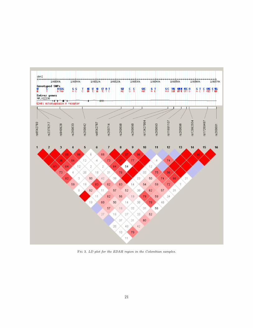
Fig 3. LD plot for the EDAR region in the Colombian samples.

21

Posterior Distribution of K

K3 4 5 6

0.0

0.2

0.4

0.6

0.8

Fig 4. EDAR data: posterior distribution of the number of clusters K.

22

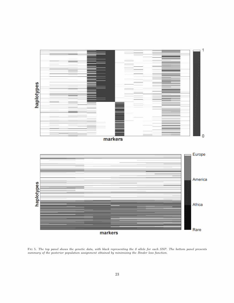
Fig 5. The top panel shows the genetic data, with black representing the 0 allele for each SNP. The bottom panel presentssummary of the posterior population assignment obtained by minimising the Binder loss function.

23

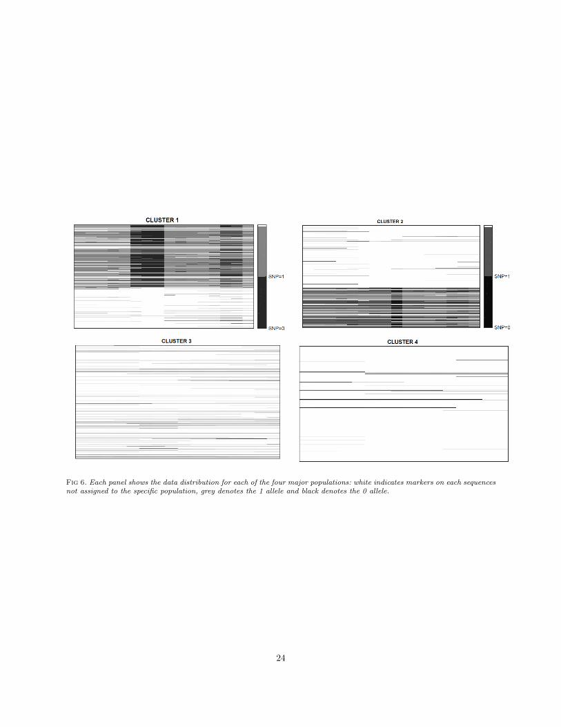
Fig 6. Each panel shows the data distribution for each of the four major populations: white indicates markers on each sequencesnot assigned to the specific population, grey denotes the 1 allele and black denotes the 0 allele.

24

0

0.2

0.4

0.6

0.8

1

1.2

1 2 3 4 5 6 7 8 9 10 11 12 13 14 15 16

SNP no.

Average allele freq. difference of each SNP - new cluster vs. the rest

-2

-1.5

-1

-0.5

0

0.5

1

1.5

2

2.5

3

1 2 3 4 5 6 7 8 9 10 11 12 13 14 15 16

SNP no.

PC3 weights for each SNP

Fig 7. Top panel: absolute value of the difference between the average allele frequency for each SNP in all the clusters and thefrequency in the rare cluster. Bottom panel: loadings for each SNP of the third PC.

25

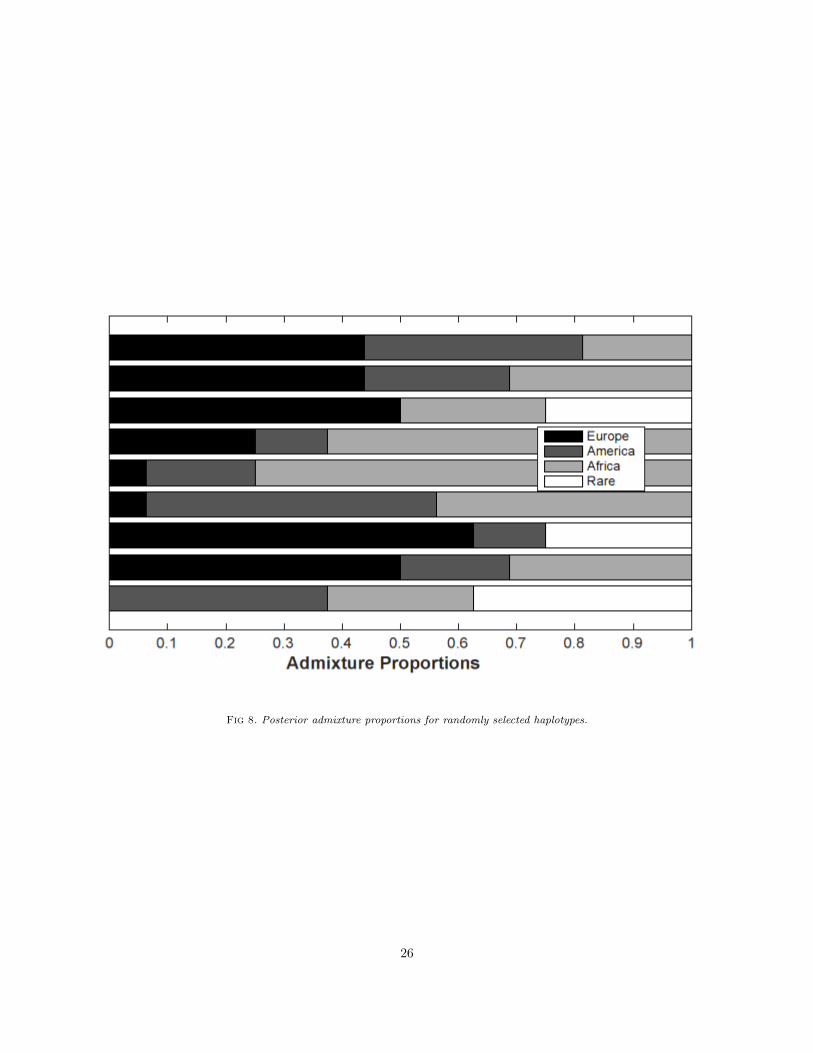
Fig 8. Posterior admixture proportions for randomly selected haplotypes.

26