Graduate Theses, Dissertations, and Problem Reports

2009

Modeling PDC cutter rock interaction Modeling PDC cutter rock interaction

Ihsan Berk Tulu West Virginia University

Follow this and additional works at: https://researchrepository.wvu.edu/etd

Recommended Citation Recommended Citation Tulu, Ihsan Berk, "Modeling PDC cutter rock interaction" (2009). Graduate Theses, Dissertations, and Problem Reports. 2054. https://researchrepository.wvu.edu/etd/2054

This Thesis is protected by copyright and/or related rights. It has been brought to you by the The Research Repository @ WVU with permission from the rights-holder(s). You are free to use this Thesis in any way that is permitted by the copyright and related rights legislation that applies to your use. For other uses you must obtain permission from the rights-holder(s) directly, unless additional rights are indicated by a Creative Commons license in the record and/ or on the work itself. This Thesis has been accepted for inclusion in WVU Graduate Theses, Dissertations, and Problem Reports collection by an authorized administrator of The Research Repository @ WVU. For more information, please contact researchrepository@mail.wvu.edu.

Modeling PDC Cutter Rock Interaction

Ihsan Berk Tulu

Thesis Submitted to the College of Engineering and Mineral Resources

at West Virginia University in partial fulfillment of the requirements

for the degree of

Master of Science in

Mining Engineering

Keith A. Heasley, Ph.D., Chair Syd S. Peng, Ph.D.

Yi Luo, Ph.D.

Mining Engineering Department

Morgantown, West Virginia 2009

Keywords: Numerical Modeling, Single Cutter Tests, Cutter Rock Interactions, FLAC3D

Abstract

Modeling PDC Cutter Rock Interaction

Ihsan Berk Tulu

Optimizing the drilling performance in high pressure high temperature (HPHT) operations is crucial to successful, economic mineral extraction, and is one of the major goals behind the Department of Energy’s (DOE) “Deep Trek” program and the primary goal of the Ultra-Deep Drilling Simulator (UDS) laboratory currently being designed and constructed at National Energy Technology Laboratory (DOE-NETL).

To best leverage the valuable unique data from experiments in the UDS, a three-dimensional FLAC model of a single cutter interacting with the rock specimen (as tested in the UDS) has been developed. This cutter-rock model was developed using parameters so that various aspects of the model could be easily changed in subsequent runs.

This study will present the development of the cutter-rock model and the results of the initial numerical tests investigating the effect of various geologic and drilling parameters such as: rock strength, pore pressure, stress fields and cutting depth. Also, the results of the comparison/calibration of the model with single cutter laboratory tests will be presented.

Three basic initial models were run. First, two different rock types (a sandstone and a shale) with three different cutting depths are modeled to investigate the effect of rock strength and cutting depth on cutter loads. Second, The effect of various confining stress levels on the single cutter tests are analyzed by applying three different hydrostatic confinements (0 MPa, 25 MPa, and 50 MPa) to the core. Third, to incorporate the effects of fluid (both drilling mud and internal fluid) on the drilling process, pore pressure is included in the cutter/rock model. Results of these models showed that initial cutter/rock model is working properly.

The calibration of the 3D numerical model with the laboratory single cutter tests was primarily accomplished by matching the average vertical and horizontal loads on the cutter between the model and the laboratory tests. A FLAC 3D model was developed to back analyze the linear cutter test data published by Glowka (1989). The model eventually calculated the cutter loads pretty close to the test results. It is found that the different failure modes in the cutter/rock model, shear (crushing) and tensile (chipping), are highly dependent on the depth of cut and the tensile strength of the rock and greatly affect the cutting loads.

iii

To my Family,

iv

ACKNOWLEDGMENTS

First of all, I would like to express my gratitude to my supervisor Dr. Keith A.

Heasley whose knowledge, leadership, professionalism, attention to detail and hard work

have set an example I hope to match some day. He provided me direction, technical

support and became more of a mentor than a professor throughout my graduate study. I

want to thank to him for giving me the opportunity to work with him and studying in

West Virginia University.

This study was performed in support of the Department of Energy’s National Energy

Technology Laboratory’s on-going research in High-Pressure High-Temperature Drilling

under the RDS contract DEAC26-04NT41817. I would like to thank you Mr. Dave Lyons

and the DOE-NETL for their support in this project.

I would like to thank Dr. Ismet Canbulat whose hard work, knowledge,

professionalism, determination and friendship have set an example for me and I would

like to thank him for his support since our first met in Johannesburg South Africa.

Most of all I would like to thank my father Ayhan, my mother Nesrin and my

sister Bengisu for their support and love.

Finally, to my dearest, beautiful, lovely fiancé Delal for her encouragement, patience,

support and making everything more meaningful and beautiful for me.

v

TABLE OF CONTENTS

ABSTRACT ........................................................................................................................ ii

ACKNOWLEDGMENTS ................................................................................................ iv

TABLE OF CONTENTS ................................................................................................. v

LIST OF FIGURES ........................................................................................................ vii

LIST OF FIGURES ....................................................................................................... viii

LIST OF TABLES ............................................................................................................ix

LIST OF SYMBOLS & ABBREVIATIONS ..................................................................x

1 INTRODUCTION.......................................................................................................... 1

2 LITERATURE REVIEW ............................................................................................. 3

2.1 THE MECHANICAL BEHAVIOR OF THE ROCK AND THE EFFECT OF

ENVIRONMENTAL CONDITIONS ........................................................................................ 3

2.1.1 The Effect of Confining Pressure .................................................................... 3

2.1.2 The Effect of Pore Fluid Pressure .................................................................. 5

2.2 BOTTOM-HOLE STRESS FACTORS AFFECTING DRILLING ..................................... 7

2.3 POLYCRYSTALLINE DIAMOND COMPACT (PDC) BITS ........................................... 9

2.4 SINGLE CUTTER TESTS ........................................................................................ 11

2.5 NUMERICAL MODELS ......................................................................................... 13

3 METHODOLOGY AND DEVELOPMENT OF FLAC3D MODEL ..................... 16

3.1 UDS GEOMETRY AND BOUNDARY CONDITIONS ................................................ 19

3.2 FLAC3D REVIEW .............................................................................................. 21

3.3 DEVELOPMENT OF FLAC3D MODEL FOR UDS SIMULATION ............................ 23

3.3.1 Grid Generation ............................................................................................ 23

3.3.2 Contact Interface .......................................................................................... 25

3.3.3 Boundary (Loading) Conditions ................................................................... 27

3.3.3.1 Axial Load ................................................................................................ 27

3.3.3.2 Rotational Load ......................................................................................... 28

vi

3.3.3.3 Cutter Reaction Forces .............................................................................. 28

3.3.4 Material Model ............................................................................................. 28

3.3.5 Modeling Approach ...................................................................................... 31

4 VERIFICATION OF THE FLAC3D UDS MODEL ................................................ 33

4.1 VERIFICATION OF THE CUTTER/ROCK INTERACTION MODEL WITH DIFFERENT

ROCK STRENGTHS AND CUTTING DEPTHS ..................................................................... 33

4.2 VERIFICATION OF THE CUTTER ROCK INTERACTION MODEL WITH DIFFERENT

STRESS FIELDS ............................................................................................................... 38

4.3 VERIFICATION OF THE CUTTER/ROCK INTERACTION MODEL WITH PORE

PRESSURE ...................................................................................................................... 42

5 CALIBRATION OF THE 3D LINEAR CUTTING MODEL WITH LINEAR

CUTTING TESTS FROM THE LITERATURE ........................................................ 46

5.1 LINEAR CUTTING TESTS ..................................................................................... 46

5.2 LINEAR CUTTING MODEL DEVELOPMENT .......................................................... 48

5.3 CALIBRATION OF THE 3D LINEAR CUTTING MODEL WITH LINEAR CUTTING TESTS

FROM THE LITERATURE .................................................................................................. 49

5.3.1 Crushing and Chipping of Rock by FLAC3D ............................................... 51

5.3.2 Parametric Study .......................................................................................... 53

5.3.3 CALIBRATION OF THE 3D MODEL .......................................................... 60

6 CONCLUSION ............................................................................................................ 63

REFERENCES ................................................................................................................ 67

vii

LIST OF FIGURES

FIG. 2.1 STRESS STRAIN CURVE OF TYPICAL TRI-AXIAL TEST. (1) ELASTIC REGION, (2)

INITIAL DAMAGE REGION, (3) POST-FAILURE REGION, (4) SHEARING AND SLIPPING

REGION (AFTER KOU ET AL., 1990) .............................................................................. 4

FIG. 2.2 SCHEMATIC REPRESENTATION OF SOIL COMPACTION (AFTER TERZAGHI, 1948) ..... 6

FIG. 2.3 BOTTOM-HOLE CONDITIONS DURING DRILLING ....................................................... 8

FIG. 2.4 PDC BITS .............................................................................................................. 10

FIG. 2.5 A) MATRIX BODY BIT, B) STEEL BODY BIT, C) STUD CUTTER (AFTER FEENSTRA,

1988) ......................................................................................................................... 10

FIG. 2.6 DEPTH OF CUT VERSUS CUTTER LOAD (AFTER RICHARD ET AL., 1998) ................. 12

FIG. 3.1 COMPUTER GENERATED RENDER OF UDS (AFTER LYONS ET AL., 2007) ............... 19

FIG. 3.2 A) CLOSE PICTURE OF THE PRESSURE VESSEL SHOWN ON FIGURE 1. B) HYDRAULIC

HOLDER INSIDE THE PRESSURE VESSEL. ...................................................................... 20

FIG. 3.3 SCHEMATIC OF THE SAMPLE GEOMETRY AND BOUNDARY CONDITIONS INSIDE THE

UDS........................................................................................................................... 21

FIG. 3.4 (A) THE VERTICAL SEGMENTS OF THE ROCK (B) CROSS SECTION OF THE ROCK (C)

TOP VIEW OF THE ROCK. ............................................................................................. 24

FIG. 3.5 (A) CUTTER GEOMETRY, (B) CUTTER ON THE ROCK .............................................. 24

FIG. 3.6 SCHEMATIC OF CONTACT INTERFACE FORMULATION. ........................................... 26

FIG. 3.7 IDEALIZED RELATION FOR DILATION ANGLE, Ψ, FROM TRIAXIAL TEST RESULTS

(AFTER VERMEER AND DE BROST, 1984) ................................................................... 30

FIG. 3.8 APPROXIMATION OF THE LINEAR SEGMENTS FOR POST FAILURE REGIME A)

COHESION B) INTERNAL FRICTION ANGLE (AFTER ITASCA, 2007) ............................... 31

FIG. 3.9 SCHEMATIC OF THE MODELING APPROACH ........................................................... 32

FIG. 4.1 TANGENTIAL LOAD ON THE PDC (SANDSTONE). ................................................... 35

FIG. 4.2 VERTICAL LOAD ON THE PDC (SANDSTONE). ....................................................... 36

FIG. 4.3 TANGENTIAL LOAD ON THE PDC (SHALE). ........................................................... 36

FIG. 4.4 VERTICAL LOAD ON THE PDC (SHALE) ................................................................ 37

FIG. 4.5 HORIZONTAL LOAD ON THE BIT FOR DIFFERENT CONFINING STRESSES. ................. 41

FIG. 4.6 VERTICAL LOAD ON THE BIT FOR DIFFERENT CONFINING STRESSES. ...................... 41

viii

FIG. 4.7 COMPARISON OF THE VERTICAL LOAD ON THE CUTTER WITH A CHANGE IN PORE

PRESSURE. .................................................................................................................. 44

FIG. 4.8 COMPARISON OF THE HORIZONTAL LOAD ON THE CUTTER WITH A CHANGE IN PORE

PRESSURE. .................................................................................................................. 45

FIG. 5.1 TEST RESULTS USED FOR CALIBRATION OF THE FLAC3D MODEL. ........................ 47

FIG. 5.2 HORIZONTAL LOAD OVER VERTICAL LOAD RATIO FOR DIFFERENT DEPTH OF CUT. 48

FIG. 5.3 ILLUSTRATION OF THE SINGLE CUTTER MODEL GEOMETRY AND BOUNDARY

CONDITIONS. .............................................................................................................. 49

FIG. 5.4 CHIP FORMATION BY FLAC3D ............................................................................. 51

FIG. 5.5 AVERAGE VERTICAL LOAD ON CUTTER VERSUS DEPTH OF CUT (INITIAL MODEL) . 52

FIG. 5.6 VERTICAL LOAD VERSUS INTERFACE FRICTION ANGLE AT VARIOUS DEPTHS OF CUT.

................................................................................................................................... 56

FIG. 5.7 HORIZONTAL LOAD VERSUS CONTACT INTERFACE FRICTION AT VARIOUS DEPTHS OF

CUT. ........................................................................................................................... 57

FIG. 5.8 VERTICAL LOAD VERSUS DILATION ANGLE AT VARIOUS DEPTHS OF CUT. .............. 58

FIG. 5.9 HORIZONTAL LOAD VERSUS DILATION ANGLE AT VARIOUS DEPTHS OF CUT. ......... 58

FIG. 5.10 VERTICAL LOAD VERSUS DEPTH OF CUT FOR TENSILE STRENGTHS: 15MPA,

30MPA AND 45MPA. ................................................................................................. 59

FIG. 5.11 HORIZONTAL LOAD VERSUS DEPTH OF CUT FOR TENSILE STRENGTHS: 15MPA,

30MPA AND 45MPA. ................................................................................................. 60

FIG. 5.12 VERTICAL LOAD VERSUS DEPTH OF CUT (CALIBRATED MODEL). ......................... 61

FIG. 5.13 HORIZONTAL / VERTICAL LOAD RATIO VERSUS DEPTH OF CUT (CALIBRATED

MODEL) ...................................................................................................................... 62

ix

LIST OF TABLES

TABLE 4.1 . MODEL GEOMETRY PARAMETERS 33

TABLE 4.2 MATERIAL PROPERTIES FOR THE ROCK SPECIMENS 34

TABLE 4.3 POST-FAILURE PROPERTIES FOR THE ROCK SPECIMENS. 34

TABLE 4.4 AVERAGE TANGENTIAL LOAD AND VERTICAL LOAD FOR SANDSTONE AND

SHALE. 38

TABLE 4.5 . MODEL GEOMETRY PARAMETERS 39

TABLE 4.6 MATERIAL PROPERTIES FOR THE ROCK SPECIMENS 39

TABLE 4.7 POST-FAILURE PROPERTIES FOR THE ROCK SPECIMENS. 39

TABLE 4.8 AVERAGE HORIZONTAL AND VERTICAL LOADS ON BIT FOR DIFFERENT CONFINING

STRESSES 40

TABLE 4.9 PEAK MATERIAL PROPERTIES 42

TABLE 4.10 POST-FAILURE (PLASTIC) PROPERTIES FOR THE ROCK SPECIMEN. 42

TABLE 4.11 AVERAGE CUTTER LOADS AND UNI-AXIAL COMPRESSIVE STRENGTH (UCS) 44

TABLE 5.1 MECHANICAL PROPERTIES OF BEREA SANDSTONE 49

TABLE 5.2 MECHANICAL PROPERTIES USED IN FLAC MODEL 50

TABLE 5.3 PARAMETRIC STUDY RESULTS 55

TABLE 5.4 POST FAILURE PROPERTIES USED IN THE FINAL FLAC MODEL. 60

x

LIST OF SYMBOLS & ABBREVIATIONS

A : Representative Area Associated with Interface Node

C : Cohesion

Co : Celsius

DEM : Discrete Element Method

DOE : Department of Energy

EDL : Extreme Drilling Laboratory

EIA : Energy Information Administration

Fo : Fahrenheit

Fn : Normal Force

Fs : Shear Force

FLAC : Fast Lagrangian Analysis of Continua

HPHT : High Pressure High Temperature

Kn : Normal Stiffness

Ks : Shear Stiffness

MMbd : Million Barrels Per Day

MPa : Mega Pascal

NETL : National Energy Technology Laboratory

P : Pore Pressure

PDC : Ploy Crystalline Diamond

PFC : Particle Flow Code

Psi : Pound Per Square Inch

ROP : Rate of Penetration

S : Applied Load

Tcf : Trillion Cubic Feet

Un : Absolute Normal Penetration of Interface Node into the Target Face

UCS : Uni-axial Compressive Strength

UDS : Ultra Deep Drilling Simulator

USGS : United Stated Geological Survey

σ1 : Maximum Principal Stress

xi

σ3 : Minimum Principal Stress

σt : Tensile Strength

σn : Normal Stress

σsi : Shear Stress

ψ : Dilation Angle

Φ :Internal Friction Angle

∆Usi :Incremental Shear Displacement Vector

1

1 Introduction

About 70% of the energy used by Americans each year comes from domestic

production. 85% of the total US energy requirement is supplied by fossil fuels and 40%

of the total energy is supplied by petroleum products (EIA, 2008). Thus, petroleum

products are a primary means for the USA to manage energy demand fluctuations.

During 2007, the United States consumed 20.7 million barrels per day (MMbd) of

petroleum products. To meet the demand, 13.5 MMbd of petroleum products were

imported. Domestic oil production of the USA supplied only 35% of this demand, and the

rest of the demand was met by importing (65%). In 2007, USA’s five biggest petroleum

suppliers were Canada (18.2% of the total petroleum import), Mexico (11.4% of the total

petroleum import), Saudi Arabia (11.0% of the total petroleum import), Venezuela

(10.1% of the total petroleum import) and Nigeria (8.4% of the total petroleum import)

(EIA, 2008). This makes the USA highly dependent on foreign countries to meet its oil

demand.

One of the best ways to become more independent of foreign energy is to increase the

domestic oil production. In the United States, there are oil and gas reserves under deep

formations which have true vertical depth greater than 15,000 feet. In 1995 the United

States Geological Survey (USGS) reported that 114 trillion cubic feet (Tcf) of

recoverable deep gas resources remains inside the USA border (USGS, 1995). However,

oil and gas production from deep formations has some difficulties. As we drill deeper

into the earth, more challenging drilling problems occur. Solving and overcoming these

problems requires more time hence more money. Experience has shown that in very deep

wells, drilling the last 10% of the well can cost as much as 50% of the total drilling cost

(Lyons et al., 2007).

There are four significant parameters that increase with the depth: rock hardness,

temperature, formation pressure and distance between the bit and the drilling control unit.

Rock hardness and abrasiveness generally increase with the depth, leading to a lower rate

of penetration (ROP). In the last 10% of the hole ROP can be as low as 4.5 ft/hr and for a

15,000 ft deep well, drilling the last 10% might take as long as 15 - 20 days or more.

Higher temperatures and higher pressures at depth along with the harder rock increase bit

wear and shorten the bit life. During drilling of deep formations, drill bits may only last

2

days or even hours. Therefore economical drilling is often not economically possible

under high pressure and high temperature (HPHT) conditions.

Optimizing the drilling performance in these HPHT operations is crucial to

successful, economic mineral extraction, and is the primary goal of the Extreme Drilling

Laboratory (EDL) and the Ultra-Deep Drilling Simulator (UDS) currently being designed

and constructed at Department of Energy – National Energy Technology Laboratories

(DOE-NETL). The UDS is a unique single cutter test machine which can simulate a

single cutter interacting with the rock formation at bottom-hole pressures up to 30,000 psi

and temperatures up to 4800F. Drilling fluid pressure, drilling fluid properties, rock

properties, pore pressure and drilling parameters (cutter rotation speed, weight on bit etc.)

are some parameters that can be studied in the extreme drilling lab and UDS (Lyons et

al., 2007).

DOE_NETL is also pursuing numerical modeling of the cutter/rock interaction to

support the UDS experiments. To best leverage the valuable unique data from

experiments in the UDS, a three-dimensional Fast Lagrange Analysis of Continuum

(FLAC3D) model of a single cutter interacting with the rock has been developed. This

3D FLAC model will be used to back analyze the experiments in the UDS and

experiments from the literature in order to calibrate, validate and optimize the simulated

rock mechanics. The validated cutter-rock model, coupled with the UDS experiments,

might then be used to analyze the influence of: temperature, pressure, formation and mud

properties, bit design and drilling parameters on the cutting process and ultimately

optimize drilling rate of penetration in HPHT conditions.

This thesis reports on the development of a three dimensional numerical model of a

single cutter interacting with the rock formation to simulated the Ultra Deep Drilling

Simulator (UDS). In the thesis, a model with the true 3D geometry of UDS sample

simulation is demonstrated to show that the model can reasonably simulate the UDS

experiments with different rock formations, stress environments and fluid pressures.

Additionally, a linear cutter model (very similar to the UDS model) is calibrated with

single cutter test data published in the literature to investigate the difficulty of calibrating

the model and the degree of fit that can be obtained between the numerical model and the

laboratory tests.

3

2 Literature Review

A lot of research has been dedicated to understand and model the mechanisms of rock

failure associated with bits and cutters. Evidently, rock cutting by bit indentation is a

basic process in wellbore drilling (and mechanical mining) and an accurate prediction of

the rock cutting process can help to optimize the drilling operation and the drill bit

design. However, bit-rock interaction is not a simple process. The natural rock properties

and failure process are not as well understood as those for man-made materials and at the

bit tip, the effects of high strain rates, confining pressure and pore pressure greatly

complicate the understanding and analysis of the rock failure. Three aspects, which are:

the mechanical behavior of the rock, the bottom-hole conditions and the characteristics of

the mechanical tool, need to be identified in order to accurately model the cutter/rock

interaction during the drilling operation.

2.1 The Mechanical Behavior of the Rock and the Effect of

Environmental Conditions

Mechanical properties of the rock like materials are strongly influenced by their

environment. Kou (1995) identified the four major factors affecting the behavior of the

rocks. These are confining pressure, pore fluid pressure, temperature and loading rate.

The effect of temperature and loading rate are not in the scope of this study; however, the

next two sections explain the effect of confining pressure and pore fluid pressure on the

mechanical behavior of a rock.

2.1.1 The Effect of Confining Pressure

The behavior of the rock, when exposed to confining pressure, has been the subject of

the much research. A tri-axial test, which measures the compressive strength of the rock

under confining pressure, is commonly used to investigate the effect of confining

pressure on rock failure. During this test, a cylindrical rock specimen is placed into the

tri-axial cell and a constant compressive confining pressure is radially applied to the

4

specimen. At the same time, an increasing axial load is applied at the top of the specimen

until the rock fails. Figure 2.1 shows a typical stress versus strain curve of a tri-axial test.

Kou et al. (1990) analyzed the behavior of rock subjected to confinement, by dividing

the stress-strain curve into four regions. The first region is the elastic region (see figure

2.1). In this region, the rock behaves in an elastic manner, meaning that if the specimen is

unloaded in this region, it returns back to its original state along the loading curve with

no (or very little) permanent deformation. The next region is the “initial damage region”

where micro fractures start to form (2nd region in figure 2.1). When the axial stress

reaches the compressive strength of the rock, the micro-fractures coalesce into fracture

planes. Then, the post-failure region starts (3rd region on figure 2.1). In this region, the

bearing strength of the rock declines with increased deformation, until axial strength has

reached the residual strength of the rock. At the residual strength the shearing and

slipping region starts (4th region on figure 2.1). Here, fracture planes slide along each

other with a constant frictional resistance, which is equal to the residual strength of the

rock.

Fig. 2.1 Stress strain curve of typical tri-axial test. (1) Elastic region, (2) initial damage

region, (3) post-failure region, (4) shearing and slipping region (after Kou et al., 1990)

5

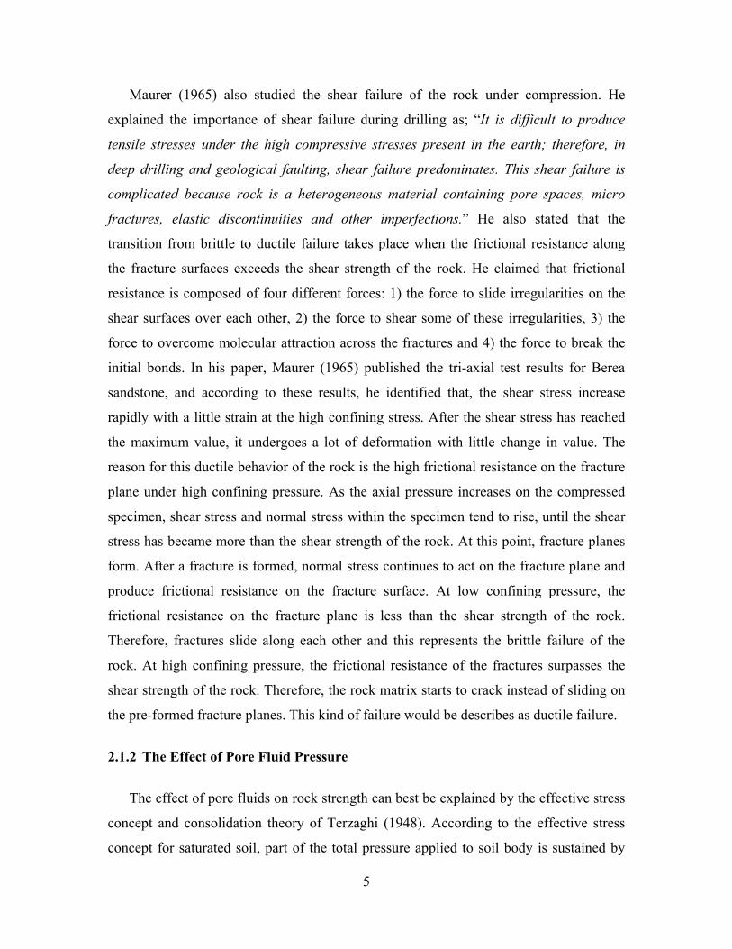
Maurer (1965) also studied the shear failure of the rock under compression. He

explained the importance of shear failure during drilling as; “It is difficult to produce

tensile stresses under the high compressive stresses present in the earth; therefore, in

deep drilling and geological faulting, shear failure predominates. This shear failure is

complicated because rock is a heterogeneous material containing pore spaces, micro

fractures, elastic discontinuities and other imperfections.” He also stated that the

transition from brittle to ductile failure takes place when the frictional resistance along

the fracture surfaces exceeds the shear strength of the rock. He claimed that frictional

resistance is composed of four different forces: 1) the force to slide irregularities on the

shear surfaces over each other, 2) the force to shear some of these irregularities, 3) the

force to overcome molecular attraction across the fractures and 4) the force to break the

initial bonds. In his paper, Maurer (1965) published the tri-axial test results for Berea

sandstone, and according to these results, he identified that, the shear stress increase

rapidly with a little strain at the high confining stress. After the shear stress has reached

the maximum value, it undergoes a lot of deformation with little change in value. The

reason for this ductile behavior of the rock is the high frictional resistance on the fracture

plane under high confining pressure. As the axial pressure increases on the compressed

specimen, shear stress and normal stress within the specimen tend to rise, until the shear

stress has became more than the shear strength of the rock. At this point, fracture planes

form. After a fracture is formed, normal stress continues to act on the fracture plane and

produce frictional resistance on the fracture surface. At low confining pressure, the

frictional resistance on the fracture plane is less than the shear strength of the rock.

Therefore, fractures slide along each other and this represents the brittle failure of the

rock. At high confining pressure, the frictional resistance of the fractures surpasses the

shear strength of the rock. Therefore, the rock matrix starts to crack instead of sliding on

the pre-formed fracture planes. This kind of failure would be describes as ductile failure.

2.1.2 The Effect of Pore Fluid Pressure

The effect of pore fluids on rock strength can best be explained by the effective stress

concept and consolidation theory of Terzaghi (1948). According to the effective stress

concept for saturated soil, part of the total pressure applied to soil body is sustained by

6

the “soil skeleton” of the specimen and part of it is sustained by the pore fluid. Terzaghi

(1948) explained consolidation theory and the effective stress concept with a physical

model. In this model, there is a cylindrical tube filled with water and containing metal

plates combined with metal springs as shown in figure 2.2. In this model, the springs

denote the skeleton of soil and the water denotes the pore fluid inside the pores of the

skeleton. Upon the application of pressure to the uppermost plate, the height of the

springs between the plates remains unchanged as long as no water escapes from the

system. Terzaghi (1948) said that in the initial loading stage the applied pressure is

supported entirely by the equal and opposite pressure of the water. Therefore, the ratio

between total applied pressure and the pore fluid pressure is equal to one. As water is

allowed to escape from the system, the plates move down and the springs start to carry

part of the applied load. As more and more water flows out from the system, the springs

carry a greater share of the applied load. After a sufficient amount of water has escaped

from the system, the percentage of the total applied load carried by the resistance of the

springs and resistance of water pressure stays constant.

Fig. 2.2 Schematic representation of soil compaction (after Terzaghi, 1948)

Although rocks are different than soils in many ways, the effective stress concept and

consolidation theory can still explain the response of the rock to the pore pressure. When

load is applied to a permeable rock, water can escape from it. If the rock is impermeable,

the water will not escape from the pores and it will be squeezed inside the pore.

Therefore, there would be a high excess pore pressure inside the rock.

7

In the paragraphs above it is shown that the environmental factors of confining

pressure and pore pressure can greatly affect the mechanical behavior of rock. These

factors might be seen during the well drilling. Therefore, understanding the effect of the

local pore pressure and in-situ stresses at the bottom of the oil well (bottom-hole) during

the rock cutting on drilling efficiency is crucial for understanding the cutter-rock

interactions.

2.2 Bottom-Hole Stress Factors Affecting Drilling

Optimizing the drilling ROP and understanding the drill bit and rock interaction

require detailed knowledge of the bottom-hole environment. Figure 2.3 shows the

bottom-hole stresses components for a vertical well: 1) overburden or formation pressure,

2) pore fluid pressure and 3) drilling fluid (mud) pressure. During drilling, drilling fluid

(commonly called mud) is pumped from the surface to the bottom of the hole and this

fluid fills the annulus of the well bore. This drilling fluid is used for removing the cutting

chips, cooling the bit and equalizing the borehole wall pressure to help preventing the

failure of the borehole wall. In the current drilling industry, a main design criterion for

drilling mud is for protection of the well bore stability.

8

Fig. 2.3 Bottom-hole conditions during drilling

Warren and Smith (1985) explained the effect of bottom-hole stress factors while

drilling. They stated that the rate of penetration (ROP) obtained during drilling operations

decreases with increasing depth. The reasons for this decrease are stated as: an increase in

differential pressure between local in-situ pore fluid pressure and mud pressure, an

increase in mud pressure, an increase in in-situ stresses, a decreasing porosity, and chip

hold-down (difficulty of removing the cutting chips). Additionally, they claimed that

when drilling in impermeable formations like shale the ROP is typically less than when

drilling in permeable formations like sandstone.

The change of ROP is strongly depended on differential pressure. Differential

pressure is the difference between the local in-situ pore pressure and the bottom-hole

mud pressure, generated by the weight of the drilling mud in the borehole. According to

tests results obtained from drilling Mancos shale with roller-cone bits under different

bore-hole pressures and constant atmospheric pore pressure, Warren and Smith (1985)

showed that ROP decreases with an increase in differential pressure. During these tests

differential pressure was increased by increasing the bore hole pressure on the rock.

9

Maurer (1965) stated the same comment based on an experimental study on the single-

tooth impact tests referenced by Warren and Smith (1985). In his experiments, Maurer

(1965) used a test setup which has the ability to control the overburden, bore-hole and

pore pressures changes independently during the test. When the differential pressure was

kept constant and the confining pressure (overburden pressure) increased, the volume of

the crater formed by the failure of the rock did not change. When the differential pressure

increased (bore hole pressure was increased and pore pressure was constant), the volume

of the crater decreased. Since the volume of the crater was not affected when the

differential pressure was kept constant (regardless of overburden pressure), and since the

crater size was affected by the change in differential pressure, Maurer (1965) concluded

that ROP depended on differential pressure.

Low ROP while drilling impermeable formations like shale is a one of the serious

challenges in the drilling industry. Warren and Smith (1985) gave the answer to the

question of why drilling impermeable formation require more time than permeable

formations as; strain relaxation during drilling causes an increase in the pore volume.

This increase in pore volume causes a corresponding decrease in the pore pressure of

impermeable rock, but does not affect the pore pressure of a permeable rock. The

reduction in pore pressure causes an increase in differential pressure. While drilling the

impermeable formations, differential pressure increases. On the other hand, differential

pressure stays constant during the drilling of permeable formations. A decrease in ROP is

more significant when drilling impermeable rocks because the differential pressure

between bottom-hole pressure and pore pressure control the ROP.

Warren and Armagost (1988), Warren and Sinor (1989) and Feenstra (1988) cited the

importance of the bit design on ROP and drilling efficiency. Additionally, Feenstra

(1988) gave a literature review on polycrystalline diamond compact (PDC) bits which

have dominated the drilling industry since their discovery.

2.3 Polycrystalline diamond compact (PDC) bits

PDC bits were introduced to the oil industry in 1970 by General Electric (Feenstra,

1977). Since then, their use in the oil industry has spread all over the world. A Typical

PDC drag bit consists of numerous PDC cutters mounted to the bit body (Figure 2.4).

10

Each individual cutter consists of PDC plate with a thickness of 0.5 mm built up on the

tungsten-3 mm thick carbide holding body. Individual cutter diameter can be up to 5 cm.

Fig. 2.4 PDC bits

There are two basic types of bit bodies, a steel body and a matrix body (Figure 2.5 a

b.). Cutters are placed on the stud (stud cutter) (Figure 2.5.c) and pressed into the steel

body of the steel body bits. Matrix body bits do not have any stud on them. The PDC

cutters are directly connected to the matrix body (Feenstra, 1988).

Fig. 2.5 a) Matrix body bit, b) Steel body bit, c) Stud cutter (after Feenstra, 1988)

Feenstra (1988) mentioned the importance of temperature stability on bit

performance. The temperature stability of a PDC cutter is limited. Above 7000 C, the

diamond layers might disintegrate because of the impurities inside the pores of the PDC

11

matrix (1988). This may cause micro chipping of the diamond layers. Typically the PDC

wear rate increase with temperature above 7000C.

Another factor with PDC bits that should be considered is bit balling. When drilling

impermeable formations, rock chips have a tendency to stick to the face of the PDC

cutter. Bit balling is one of the biggest problems in the drilling industry. Increasing the

hydraulic horse power may help, but it is not a guaranteed solution (Warren and

Armagost, 1988, Warren and Sinor, 1989 and Feenstra, 1988). Using larger cutters help

in cleaning the cutter surface, but this may cause higher individual cutter loads, hence

faster wear of the cutters (Warren and Armagost, 1988 and Warren and Sinor, 1989).

Effective PDC bit design is crucial for economic oil recovery. There are numerous

methods to design bits; mathematical models, numerical models, full scale bit tests, etc.

Among all of the possible methods, single cutter laboratory tests have been the key for

designing a PDC bit.

2.4 Single cutter tests

In his papers, Glowka (1989) summarized the research conducted in the Sandia

National Laboratories to foster the development of the PDC bits for geothermal drilling.

The main propose of his research was to design bits for drilling of high temperature and

high pressure rock formations. In his first paper, he explained single cutter tests

performed in the Sandia laboratories. He claimed the aim of these single cutter tests as:

“We seek a model of the PDC cutting process that will allow us to determine the

penetrating and drag forces acting on each cutter located on the bit face. The primary

parameters that affect these forces include the rock type, cutter design and wear state,

position on the bit, cutter interaction, cutting speed, rock stress state, and fluid

environment.” During the tests, both sharp and worn cutters were used. Also, the effect of

the depth of cut on the cutter forces was analyzed with the depth of cuts varying between

0.1 - 0.01 inch. Three different rocks, Berea sandstone with a compressive strength of 49

MPa, Tennessee marble with a compressive strength of 123 MPa and Sierra white granite

with compressive strength of 148 MPa, were used. Interaction between the cutters and

effect of water jet cleaning were also studied. All tests were performed under the

atmospheric pressure.

12

The Methodology and the apparatus for performing a scratch test which was designed

to measure the strength of the rocks were explained by Richard et al. (1998). In this case

a scratch test was the linear cutting of the rock by PDC bit with a constant cutting depth

and constant speed. Cutting depth is usually less than 2mm. Richard et al. (1998) stated

that there are two different failure mechanisms and these failure mechanisms are related

to the depth of cut. Crushing of the rock is observed with a small depth of cut and brittle

failure of the rock is associated with fracture propagation causing chipping of rock seen

above a certain threshold depth of cut. He demonstrated the transition from crushing to

brittle failure with the force versus depth of cut graph from scratch tests with Vosges

Sandstone (Figure 2.5). He identified three regimes on the graph. The first regime is the

crushing regime. In this regime, both peak and average forces increase linearly with the

cutting depth. The second regime is the transition zone. In this regime, the average force

increases non-linearly, but the peak force increases linearly. In the third regime, the

brittle regime, both forces increase non-linearly with the cutting depth.

Fig. 2.6 Depth of cut versus cutter load (after Richard et al., 1998)

13

2.5 Numerical Models

Numerous researchers have modeled the cutter-rock interaction (Leelasukseree,

2006). A comprehensive review on the physical and numerical modeling for modeling

disk cutters has been given by Al-Jalil (2006). He stated that plane-strain or axi-

symmetric physical and numerical models with indentors are not exactly representative of

the true 3-D field situation with dynamic normal and rolling forces and the induced

change in stress, and that the prediction methods based on these 2-D empirical and

analytical methods might under/overestimate the rate of penetration by the order of 80%

to 900%. He also recommends that prediction methods calibrated by laboratory tests give

better results. During the indentation of the rock, three zones are observed: crushed,

inelastic cracking and elastic. He lists five essential hypotheses for a good indentor

model: 1) A cavity expansion model is applicable. 2) The principles of linear elastic

fracture mechanics apply (but in the macro-scale this can be viewed as shear failure). 3)

There is an elliptical crushed zone beneath the indentor and this zone applies compressive

stresses (pressure) to the wall of the expanding cavity. 4) Microcracks exist along the

boundary between the crushed zone and the inelastic, cracked zone. These microcracks

grow and coalesce into cracks that eventually create chips. 5) Dilation occurs whenever

part of “intact” rock fails (i.e., stress point in stress space reaches the failure envelope).

Confining stress changes the direction of crack growth.

Most of the numerical analyzes in the literature are two-dimensional and the effect of

only a few parameters are analyzed (Leelasukseree et al., 2006). Validation of the

numerical models with field and/or laboratory data is sometimes performed but not often.

In additional to the continuum method (Al-Jalil, 2006, Zhang. and Roegiers, 2005,

Stavropoulou, 2006, Saouma and Kleinosky, 1984, Han et al., 2006, Han et al., 2005 and

Bruno et al., 2005), the discrete element method (DEM) has also been used for numerical

modeling (Stavropoulou, 2006, Huang et al., 1999). The FLAC code has been used for

different cutter rock interactions; drag cutting (Stavropoulou, 2006, Huang et al., 1999),

disc cutting (Leelasukseree et al., 2006) and percussive drilling (Han et al., 2006).

Stavropoulou (2006) modeled the drag cutting of a rotary bit by using both FLAC2D

(continuum method) and PFC2D (discrete element method). He also compared the

14

numerical model results with actual test data. According to his observations, the

continuum model predicted the results better than the DEM. The FLAC work by Terralog

(Han et al., 2006, Han et al., 2005 and Bruno et al., 2005) was some of the more

innovative modeling of drilling to date. In their 3D FLAC model, the percussion bit is

modeled as a pressure pulse on the formation. The rock is checked for compression,

tension and/or shear failure. When the rock is determined to be failed, the elements are

removed from the model. Also, they reduce the rock strength properties in the model due

to a “fatigue” factor which is determined from a function of the previous stress

magnitudes to which the rock has been subjected. The Terralog model is three-

dimensional and has some fairly comprehensive rock failure analysis (including

compression, tension and shear failure modes with differential pore pressures); however,

the model does not explicitly model the bit geometry. Nor does the model include any

shear or rotational bit forces. Also, the model does not determine the effective stress

(pore pressure) in the rock nor analyze failure in the effective stress realm. These factors

can be critical in accurate modeling of the rock-bit interaction.

Many previous numerical models have been very useful for analyzing certain aspects

of the cutter-rock interaction such as: crack propagation, porosity, or rock heterogeneity.

However, only a couple of them were compared with actual laboratory data

(Stavropoulou, 2006, Huang et al., 1999) and their intent was never to calibrate the model

with reality. Additionally, these models were two dimensional and they were not

representative of the actual geometry of the test setup. Two different failure mechanisms

crushing and chipping of the rock were modeled by Huang et al. (1999), and

Stavropoulou (2006) showed that chipping is possible with the FLAC2D code. However,

both of them ignored the post failure behavior and the dilatation of the rock, which can be

an important aspect of chipping (Al-Jalil, 2006).

With the Ultra-Deep Drilling Simulator (UDS), sufficient laboratory information

should be available to calibrate and validate a “realistic” cutter rock model. To obtain a

realistic simulation, the cutter-rock model will have to be three dimensional as in the

UDS. It will have to model a continuously changing contact interface between the cutter

and the rock as the bit penetrates and fails the rock matrix. And of course, a realistic

model will have to accurately model the rock properties (elastic modulus, Poisson’s

15

Ratio, cohesion, friction angle, dilation angle, porosity, permeability, accurate failure

model, etc.).

16

3 Methodology and Development of FLAC3D Model

The numerical models summarized in the previous chapter helped to identify certain

aspects like: crack propagation, the effect of pore pressure and the effect of material

properties on cutting forces. However, only a few of the previous models were validated

with laboratory data (Stavropoulou, 2006, Huang et al., 1999) and the intent of the

research was never to calibrate the model with reality. Additionally, these models were

all two dimensional; and therefore, they were not all that representative of the actual 3D

geometry of an actual laboratory test setup.

Huang et al. (1999) developed a 2D PFC model of a linear cutting test and compared

the model results with linear cutting test data (Richard et al., 1998). His model calculated

cutter loads close to the test results. Additionally, the model showed the different failure

modes of the rock, crushing and chipping, as seen in the test. An elastic, perfectly-plastic

Mohr-Coulomb failure criterion was selected as the material model. Post failure behavior

of the rock was ignored. They modeled compressive strength tests with the PFC model to

relate the micro parameters (radius of the particles, normal and shear stiffness between

particles, etc.) in the model with the macro parameters (compressive strength, elastic

modulus, fracture toughness, etc.) of the rock. The reason for modeling the compressive

strength tests was due to the lack of any empirical or analytical method for directly

relating micro parameters of the particle model to the macro properties of the rock mass.

This is a distinct drawback of the particle model and because of this necessity; accurately

modeling the post failure behavior of the rock is very hard with present particle codes.

Stavropoulou (2006) modeled drag cutting with a rotary bit by using FLAC2D (a

continuum method) and PFC2D (a particle method). He compared the thrust and torque

calculated by both models with the test data, and he concluded that the continuum model

predicted the results better than the DEM. Stavropoulou showed that chipping is possible

with the FLAC2D code, but his model only calculated the torque and thrust until the

failure of the first chip. He could not model a longer displacement of the cutter because

the continuum model does not form multiple chips that can interact the particle code.

Cutter/rock interaction models might be used to optimize the drilling operations. This

will be possible only if an accurate modeling approach, which can simulate the true

17

geometry, boundary conditions and failure mode of the rock in the actual drilling

environment, is selected. The required characteristics of a model which could be used to

accurately optimize the drilling operations is summarized as fallows;

1. The model should be three dimensional to simulate the real geometry and the true

boundary conditions encountered in the field or in a laboratory.

2. The model should be capable of modeling bottom-hole stress conditions, pore

fluid pressure, overburden pressure and mud pressure.

3. The rock material needs to accurately model the failure process under the

expected fluid pressure, in-situ stress conditions, and temperature. (Effect of

bottom-hole stress conditions on drilling is detailed in Chapter 2.)

4. The model should be capable of calculating cutter loads close to the actual field or

test data.

5. The model should have an interface between the cutter and rock, which must be

able to continuously change location as the cutter or rock moves, and the interface

must accurately transfer the normal and shear (frictional) loads between the cutter

and the rock.

6. The model should be capable of performing a parametric study to investigate the

rock parameters which are not easy to measure, but important in a cutter/rock

model such as: dilation angle or post-failure behavior.

The first three bullets detailed above require actual field or laboratory data to

calibrate a numerical model. Interpretation of actual field data to use in the calibration of

a numerical model is not easy. Therefore, using tightly controlled laboratory data will

give better information for calibration of numerical models. (Hence the need for the

UDS) There is not much published information concerning bullet two above. Research

conducted on understanding ROP as a function of various stress and fluid pressures is

concentrated on the results of full scale bit tests analyzing: different bit designs, different

drilling mud properties and different nozzle hydraulic powers. Detailed rock properties

and single cutter loads calculations are not included in these previous studies (Warren

and Armagost, 1988, Warren and Sinor, 1989). Additionally, there are not many single

18

cutter test machines that can simulate the actual drilling environment like bore hole-

pressure, pore pressure, real mud properties and removal of the chips.

In recent years, increasing demand for petroleum products and natural gas directed

the attention of the US government to the deep oil and gas reserves. Economical

extraction of deep reserves requires an understanding of the bottomhole conditions under

the HPHT environment. To address the solution of the problems under HPHT drilling

environments, DOE-NETL developed the unique single cutter test machine, the UDS.

The UDS can simulate single cutter tests under HPHT environment with real drilling

mud.

One of the main objectives of this thesis is to develop a three dimensional numerical

model of a single cutter interacting with the rock formation to simulated the tests in the

Ultra Deep Drilling Simulator and to show that the model can reasonably simulate the

UDS experiments with different rock formations, stress environments and fluid pressures.

Additionally, a linear cutter model (very similar to the UDS model) is developed and

calibrated with single cutter test data published in the literature to investigate the degree

of difficulty in calibrating the model and the degree of fit that can be obtained between

the numerical model and the laboratory tests.

This chapter explains the methods used in carrying out the thesis. Steps involved in

achieving the objectives of this thesis are as follows;

1. Investigation of the UDS to determine the three dimensional geometry and the

boundary conditions of the FLAC3D model.

2. Review of FLAC3D.

3. Development of a 3D model with a strain softening Mohr-Coulomb rock material

and a dynamic interface between the rock and a single cutter.

4. Verification of a FLAC3D model of the UDS with different rock formations, pore

pressures and stress fields.

5. Development of a FLAC3D linear cutting model to be calibrated with single

cutter test data published by Glowka (1989). Investigation of failure modes

(chipping and crushing) with calibrated model and validation of the model results

with test data (Glowka, 1989).

19

6. Performing parametric study to investigate the effect of model parameters on

cutter forces.

3.1 UDS Geometry and Boundary Conditions

Geometry and the boundary conditions of the FLAC3D model are determined

according to the paper published by Lyons et al. (2007) about the UDS. This unique

testing machine is designed by TerrTek Schlumberger. Figure 3.1 shows the computer

generated rendering of the UDS (Lyons et al., 2007).

UDS as designed to allows simulating the bottom-hole conditions of wells drilled

deeper than 15,000 feet (4.572 meters). Therefore, the UDS will be able to apply fluid

pressure up to 30,000 psi and temperature up to 481 °F. During the simulation of the

cutting process, real drilling mud will be used and cutting process inside the UDS will be

monitored by a high speed x-ray machine (Figure 3.1). X-ray system will be used during

UDS testing to visualize the pressure vessel internals.

Fig. 3.1 Computer generated render of UDS (after Lyons et al., 2007)

The test specimen is a cylindrical rock core having dimensions of 8” diameter x 12”

long. This rock specimen will be attached to a sample holder on the bottom plug that is

driven by hydraulic motor. This hydraulic holder is inside the pressure vessel (Figures 3.2

(a) and (b)). This hydraulic system provides rotational motion in the X-Y plane and linear

displacement in the Z-direction.

The UDS machine will have one or more “cutters” installed within the pressure vessel

that contacts the rock specimen. The cutter dimensions and properties are specified by the

Pressure Vessel

20

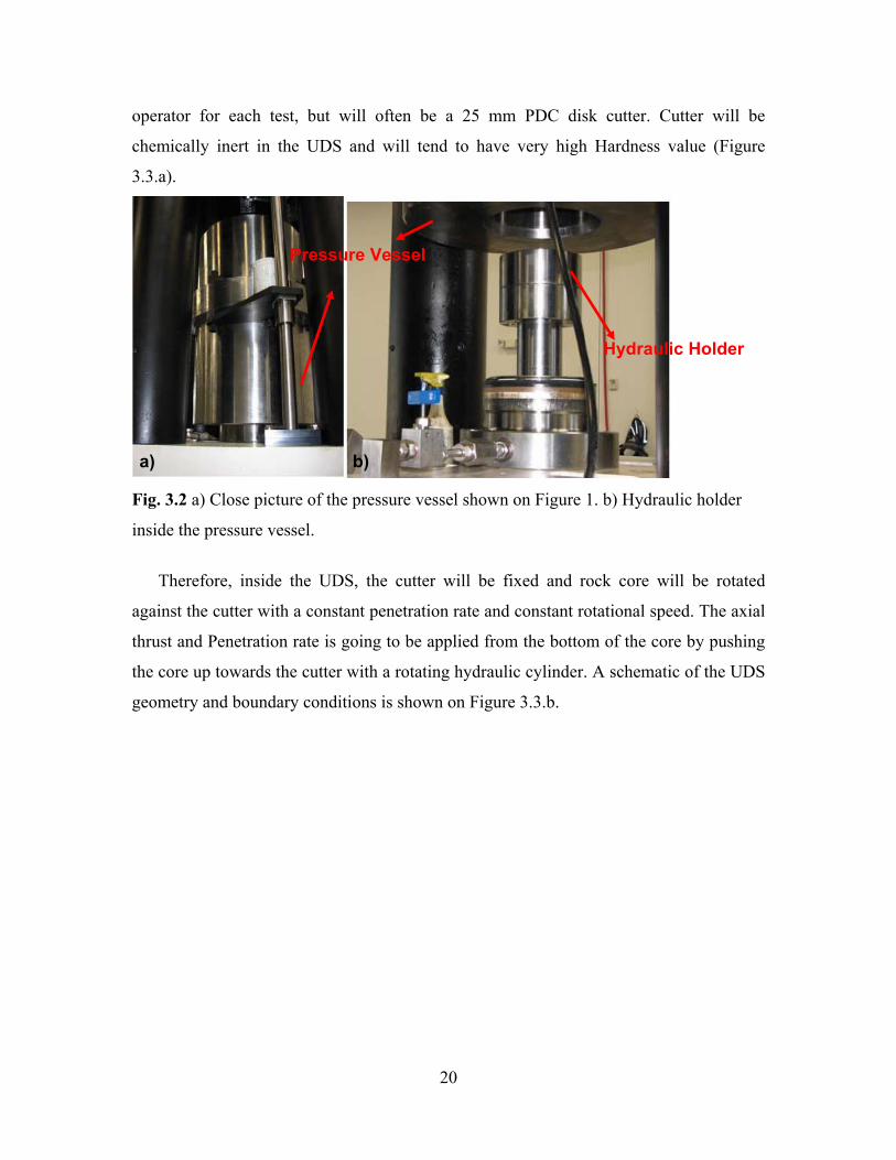
operator for each test, but will often be a 25 mm PDC disk cutter. Cutter will be

chemically inert in the UDS and will tend to have very high Hardness value (Figure

3.3.a).

Fig. 3.2 a) Close picture of the pressure vessel shown on Figure 1. b) Hydraulic holder

inside the pressure vessel.

Therefore, inside the UDS, the cutter will be fixed and rock core will be rotated

against the cutter with a constant penetration rate and constant rotational speed. The axial

thrust and Penetration rate is going to be applied from the bottom of the core by pushing

the core up towards the cutter with a rotating hydraulic cylinder. A schematic of the UDS

geometry and boundary conditions is shown on Figure 3.3.b.

a) b)

Pressure Vessel

Hydraulic Holder

21

Fig. 3.3 Schematic of the sample geometry and boundary conditions inside the UDS.

3.2 FLAC3D Review

FLAC is a finite difference program with a continuum approach primarily for

modeling of the geo-mechanical problems.Two dimensional version of FLAC was first

developed to model the geological materials (soil and rock mass) by the Itasca Consulting

Group (Itasca, 2007). FLAC3D is the extension of the two dimensional version to three

dimensions.

In FLAC, the geologic object is represented by polyhedral elements within a three

dimensional grid that is adjusted to fit the geometry of that object. Each polyhedral

element can yield and flow according to linear or non-linear stress strain laws.

Additionally, grids can deform and move by updating the location of each grid point.

FLAC uses a mixed discretization explicit scheme (Itasca, 2007) to model the plastic

collapse loads and plastic flow accurately. Mechanics of the medium is derived from the

dynamic equations of motions combined with the constitutive equations. Use of the

explicit scheme prevents having to form large stiffness matrices, and this allows large

strain simulations to be only slightly more time-consuming than small-strain run since

there is not a large stiffness matrix to be updated.

a) b)

22

FLAC has twelve basic built-in material models and these models can be divided into

three main groups (Itasca, 2007). The first model is the “null model” which is used to

simulate excavations and openings. If an element has a null model, a value of zero is

assigned to all of the stress and strain components of the element. The second model

group is the “elasticity” group. There are three different models defined in this group;

isotropic, transversely isotropic and orthotropic. The third model group is the “plasticity”

group. There are eight built-in models in this group; Drucker-Prager, Mohr-Coulomb,

strain-hardening/softening, ubiquitous-joint, bilinear strain-hardening/softening

unbiquitous-joint, double-yield, modified Cam-clay and Hoek-Brown. In this thesis, the

strain softening Mohr-Coulomb material model is primarily used. Details of this model

are explained in the next section.

FLAC has four optional features of concern to this work (Itasca, 2007). The first

optional feature is for “fluid-mechanical interaction”. The fluid-mechanical interaction

option in FLAC allows modeling groundwater flow and pore pressure dissipation, with

full mechanical coupling between a deformable porous solid matrix and the viscous fluid

flow. In FLAC, there are thee pore pressure application strategies; constant pore pressure,

mechanically-driven pore pressure and fully-coupled mechanical and fluid flow analysis

of pore pressure. Second optional feature in FLAC which is useful for this thesis is the

“thermal” option. This option allows modeling of thermal-mechanical coupled and

thermal-ground water coupled models. Third optional feature of the FLAC is the “creep

model”. Long term loading of the material can be modeled by using this option. Fourth

optional feature of the FLAC is the user defined option. By using this option user defined

constitutive model might be programmed in to the FLAC with C++ programming

language.

One of the biggest advantages of using the FLAC for modeling of the cutter-rock

interaction is its FISH feature (Itasca, 2007). FISH (Flac-ISH) is a programming language

embedded within FLAC which enables the user to defined new variables and functions

for controlling the FLAC model. Using FISH, the user can obtain and modify all of the

information in the each grid zone and the grid point in the continuum body.

23

3.3 Development of FLAC3D Model for UDS Simulation 3.3.1 Grid Generation

The main purpose of developing the three dimensional FLAC model is to use the

model in the future to calibrate with the UDS experiments. Therefore, for the FLAC3D

model development, it was desired to make the model parametric, so that the cutter size,

cutter angle, cutter thickness, cutter location, rock specimen size, specimen length and the

element sizes can be easily changed from one test geometry to the next. Also, it was

desired to systematically vary the grid densities such that the area under the cutter would

have the densest grid and the grid densities would then decrease away from the cutter in

order to help minimize the number of elements and the associated run times.

Parametric grid generation is performed for the rock specimen and the cutter

separately. The rock specimen is divided into grids as a cylinder. The grid design consists

of three segments in the vertical direction with consistent element sizes within each

segment and with the grid density increasing towards the top of the model (Figure 3.4

(a)). The element size jumps between segments in the vertical direction were kept at a

factor of two in order to minimize stress concentrations. If the element size jumps

between the segments approaches four or more, then stress concentrations can be seen

between the sections. A similar segmented approach is used for generation of the grids in

the radial direction. The rock core was eventually divided into five cylindrical segments

in the radial direction (Figure 3.4 b and c). The middle cylindrical segment, which is in

contact with the cutter, has the smallest zone. Then, the grid density decreases in the

segments toward the center of the core and towards the perimeter of the core (see Figure

3.4). Similar to the vertical direction, the element size jumps between segments in the

radial direction were kept at a factor of two in order to minimize stress concentrations.

24

Fig. 3.4 (a) The vertical segments of the rock (b) cross section of the rock (c) top view of

the rock.

The cutter grids are also designed as a cylinder to represent the round Poly Crystalline

Diamond (PDC) drag bits used in the drilling industry. The cylinder for the cutter has two

vertical segments. The thin segment with the highest grid density is intended to represent

the PDC insert at the tip of the bit, while the remainder of the cylinder with a lower grid

density is intended to represent the tungsten-carbide backing for the PDC (Figure 3.5 a

and b). For the cutter model, the length, diameter, PDC thickness, grid density and cutter

angle were all input as parameters so that they can be easily modified to match the UDS

test or any specific scenario.

Fig. 3.5 (a) Cutter geometry, (b) Cutter on the rock

25

3.3.2 Contact Interface

The contact interface between the rock and the cutter plays a very important role in

the numerical simulation of rock cutting. The interface between the cutter and the rock

specimen must be able to continuously change locations as the cutter or rock moves, and

the interface must accurately transfer the normal and shear (frictional) loads between the

cutter and the rock.

In the interface formulation, a “soft” contact is used where the interface elements are

allowed to interpenetrate the contact target face. Contact forces in the normal and shear

directions are determined by the magnitude of interpenetration and the defined stiffness

of contact springs (Figure 3.6). Therefore, the interface has the properties of Coulomb

sliding with: friction angle, normal and shear stiffnesses. The shear forces are limited by

the friction angle and the applied normal force. During each timestep, the absolute

penetration and relative shear velocity are calculated for each interface node and its

contacting target face. These values are then used to calculate an updated normal force

and shear force vector. Once the forces are determined for any given node penetration,

they are distributed over the adjacent nodes in the penetrated element in a distanc e

weighted fashion. In our rock-cutter model, the interface is applied to the PDC part of

the bit.

26

Fig. 3.6 Schematic of contact interface formulation.

The normal and shear forces that describe the elastic interface response are

determined at calculation time (t + ∆t) using the following relations:

AsiσAt))2

1((tsi∆usk(t)

siF∆t)(tsiF

AnσAnunk∆t)(tnF

+∆+

+=+

+=+

(3.1)

Where:

∆t) (t at time force Normal :∆t)(tnF ++

∆t) (t timeatvectorforceShear: F ∆t) (t si ++

facetargettheintonodeinterfaceofnpenetrationormalAbsolute:un

vectorntdisplacemeshearrelativeInremental:∆usi

Sy

Kx

Z

X

Y

F = K x D F: Force D: Displacement K: Stiffness

Ky Kz Sx

27

tioninitializastressinterfacetodueaddedstressnormalAdditional:σn

stiffnessNormal:kn

stiffnessShear:SK

tioninitializastressinterfacetoduevectorstressshearAdditional:σsi

nodeinterfacethewithassociatedareativeRepresenta:A

The Coulomb shear-strength criterion limits the shear force by the following

relationship shown in Equation 3.2. If the applied shear force become larger than the

maximum allowable shear force given by equation 3.2, then sliding is assumed to occur,

and the applied shear force stays constant and equal to the maximum shear force.

pA)(FtanφcAF nmax −+= (3.2)

3.3.3 Boundary (Loading) Conditions

3.3.3.1 Axial Load The boundary or loading conditions on the model are an area which required some

development to get exactly what was desired. For the axial load (or thrust) on the rock

specimen, a constant velocity is applied to the bottom of the core in the vertical direction.

This velocity boundary condition is a much more stable method of loading the core than

directly applying a pressure or force, particularly with strain softening and failing

elements. With an applied pressure or force, as the elements fail under the cutter, the core

will accelerate upwards and dynamic stresses will be generated by the core slamming into

the cutter. With an applied velocity to the specimen, these dynamic movements of the

core are eliminated and the model solutions are more stable.

The one down side of using a velocity boundary condition is that the load or pressure

on the rock specimen is not inherently available. With the velocity boundary condition,

the load and/or pressure on the rock specimen has to be calculated by summing the

reaction forces on all of the nodes on the bottom of the rock. For the model, a FISH

function was written to calculate the applied load due to the velocity boundary condition.

28

3.3.3.2 Rotational Load FLAC does not have a pre-defined rotational boundary condition. In order to rotate

the core, a constant linear velocity is applied to the nodes on the outer edge of the bottom

of the core, and the center nodes of the core are fixed in the horizontal directions. This

combination of boundary conditions causes the core to rotate; however, as the core

rotates, the applied velocities also have to rotate in order to stay perpendicular to the edge

of the core. A FISH function was written to rotate the applied velocity boundary

conditions as the core turns. Also a FISH function was written to sum the rotational

reaction forces and calculate the applied torque due to the rotational velocity boundary

conditions.

3.3.3.3 Cutter Reaction Forces In the cutter-rock model, the rock specimen moves upward and spins, while the cutter

bit remains stationary. To fix the cutter in the model, the nodes on the circular back

surface of the bit are fixed in the X, Y, and Z directions. In order to monitor the forces on

the bit during the cutting process, the reaction forces on the fixed nodes on the back of

the bit are summed in all three principal directions by using a FISH function. These total

reaction forces can then be compared with the axial load and rotational torque to verify

the model results.

3.3.4 Material Model

Accurate calculation of the rock failure behavior in the model is critical to modeling

the behavior of the entire cutter-rock system accurately. In this thesis, only the failure

models built into FLAC3D were utilized to see if the selected failure criterion can model

the cutter loads correctly. In this thesis, the cutter-rock model uses the strain-softening

Mohr-Coulomb plasticity material. With the strain-softening Mohr-Coulomb model, once

failure is reached for a given initial cohesion and friction angle (and pore pressure), the

material behaves plastically and starts to accumulate plastic strain. In this strain softening

material, the post-failure values of the cohesion, friction angle and dilation angle can be

input as functions of the plastic strain.

29

The Mohr-Coulomb model in FLAC3D uses a shear yield function and a tensile

cutoff. The Mohr-Coulomb criterion in FLAC3D is expressed in terms of the three

principal stresses and strains. The equation for the Mohr-Coulomb failure surface is given

as:

φφσσ NcNPPf 2)()( 31 +−+−−= (3.3)

where:

φφ

φ sin1sin1

−+

=N (3.4)

and

σ1 = major principal stress (compression is positive)

σ3 = minor principal stress

φ = internal friction angle

c = cohesion

P = pore pressure

If equation 3.3 is equal to zero or less than zero, shear yield is detected and plastic

strain starts to form according to a non-associated flow rule. When the normal stress

becomes tensile, the Mohr-Coulomb criterion loses its physical validity. At this point, the

tensile cut off function given in equation 3.5 is used. If the value of this equation is larger

than zero, tensile yield is detected. (σt is tensile strength of the rock)

tf σσ −= 3 (3.5)

After the initiation of plastic yielding, post-failure behavior of the geological material

starts. This behavior is defined by the post-failure parameters. In FLAC3D there are four

parameters with post failure properties; shear dilatancy, shear hardening/softening,

volumetric hardening/softening and tensile softening. In this study, shear dilatancy and

shear softening of the rock is used.

30

Shear dilatancy is the change in the volume of the material after shear failure.

Dilatancy is characterized by the dilation angle which is estimated from the triaxial or

shear-box tests. The dilation angle is measured from the slope of the volumetric strain

versus axial strain line in the plastic regime of the plot gathered from the triaxial test

(Figure 3.7).

Fig. 3.7 Idealized relation for dilation angle, ψ, from triaxial test results (after Vermeer

and de Brost, 1984)

Shear softening of the rock can be defined by the user by dropping the values of the

cohesion, internal friction angle and dilation angle after the failure of the rock. A table

function in FLAC3D allows the user to drop these values linearly between the specified

plastic strain percentages (Figure 3.8) (Itasca, 2007). There is not any empirical way to

determine how to mobilize these values. Gathering the post failure parameters from the

triaxial test is possible. However, there is not much available information in the literature

about the values to use for these post-failure parameters.

31

Fig. 3.8 Approximation of the linear segments for post failure regime a) cohesion b)

internal friction angle (after Itasca, 2007)

3.3.5 Modeling Approach

To simulate complete failure of the material and removal of the “chips”, once the

rock material reaches a pre-determine amount of plastic strain at a given element, that

element is changed to a “null” material and essentially removed from the model. This

approach allows us to model cutter rock interaction more realistically. Moreover, it also

allows us to observe dynamic cutter loads in the model as observed in practice.

The process of building the grids, applying material properties, applying boundary

conditions, running the model, calculating failure, removing elements, and saving

calculated boundary forces is diagramed in Figure 3.9. As shown in this figure, the

completed FLAC3D model is time-stepped for the solution. In the cutter-rock model

during the time-stepping: the load, compressive stress and displacement at the bottom of

the core; the tangential, radial and vertical loads on the PDC cutter; and the torque on the

core are calculated and stored every 50 steps. These stored values (or “histories” as they

are known in FLAC) allow the results of the model to be fully analyzed.

The FLAC continuum model can simulate the propagation of the crack and formation

of chip, but it might not form an actual discrete chip separated from the continuum

geometry. This inability to accurately model chips is one drawback of using a continuum

model to simulate the cutter/rock interaction. In FLAC, the propagation of a crack is

possible by through strain localization (which might be observed by using relatively

small elements). The strain-softening Mohr-Coulomb failure criterion in FLAC3D allows

32

this strain localization (or shear banding) to occur (shear bands) (Itasca, 2007). As

mentioned earlier in this chapter, Stavropoulou (2006) showed the formation of a chip

with FLAC2D. However, he could not model a longer displacement of the cutter.

Accurately modeling rock cutting requires the movement of the cutter for a relatively

long distance and the production of multiple chips.

Fig. 3.9 Schematic of the modeling approach

Grid generation (cutter and core)

Applying Boundary Conditions • Loading from the bottom of the core • Rotation of the core • Fixing the cutter

Assigning Material models and material properties • Elastic PDC • Strain softening (Mohr-Coulomb) rock

core

Interface Generation

Time Step Monitoring plastic strain

of the rock zones

If > 0.3 remove the

zone

If < 0.3 continue

loading

Monitoring • Core Displacement • Core Pressure • Core Torque • Load on the cutter • Physical state of the

core

33

4 Verification of the FLAC3D UDS Model

Verification of the UDS model was performed in the following order: 1) the UDS

model was first run to investigate two different rock types (a sandstone and a shale) with

three different cutting depths (penetration rates). 2) Then the UDS model was run to

investigate the effect of different hydrostatic confining pressures 3) And finally, the UDS

model was run to investigate the effect of different pore pressures.

4.1 Verification of the Cutter/Rock Interaction Model with Different

Rock Strengths and Cutting Depths

To verify the applicability of the cutter/rock model, the initial runs of the FLAC3D

model were used to investigate two different rock types (a sandstone and a shale) with

three different cutting depths (penetration rates Input parameters for the model geometry,

material model properties and strain-softening properties are summarized below in Table

4.1, Table 4.2 and Table 4.3.

For these initial numerical tests, the model cutting depth was set by initially sumping

the cutter into the rock at a constant velocity for a given number of steps to the desired

depth. Then, for the subsequent rotation of the rock specimen, the grid points at the

bottom of the core were fixed in the vertical direction. During the time-stepping for the

FLAC3D solution, the load, compressive stress and displacement at the bottom of the

core; the tangential, radial and vertical loads on the PDC cutter are calculated and stored

every 50 steps. These stored values (or “histories” as they are known in FLAC) allow the

results of the model to be fully analyzed.

Table 4.1 . Model geometry parameters

Core Length

(m)

Core Dia.

(m)

PDC

Thickness

(m)

PDC Dia.

(m)

Cutter Rake

Angle

Parameter

Value 0.4 0.2 0.0033 0.014 30o

34

Table 4.2 Material properties for the rock specimens Material Parameter Shale Sandstone

Bulk Modulus (GPa) 8.8 26.8

Shear Modulus (GPa) 4.3 7.0

Friction Angle 14.4º 27.8º

Cohesion (C) (MPa) 27.2 38.6

Dilation Angle 12.0º 10.0º

Tensile strength (MPa) 0.6 1.2

Table 4.3 Post-failure properties for the rock specimens.

Shal

e

Plastic Strain

0.00 0.05 0.10 1.00

Friction Angle 14.4º 12º 10º 10º

Cohesion (MPa) 27.2 15 1 1

Dilation Angle 12.0º 5º 0º 0º

Sand

ston

e

Plastic Strain

0.00 0.05 0.10 1.00

Friction Angle 27.8º 25º 23º 23º

Cohesion (MPa) 38.6 19 1 1

Dilation Angle 12.0º 5º 0º 0º

In Figure 4.1, the tangential forces on the bit and in Figure 4.2, the vertical force on

the bit for the different cutting depths in the sandstone are shown. Looking at the

resultant forces on the PDC cutter in these figures, one can see that the values are fairly

dynamic. In the model, the cutter is moving through the rock, and as certain elements

reach failure and are nulled, the stress levels on the cutter drop significantly. Then the

cutter starts to stress the next element and the stresses rises again until rock failure. This

cycle is repeated several times in the plots. In both of these plots, the vertical and

tangential loading cycles seem to track each other fairly well. These same types of sharp

jumps in cutter stress are also seen in laboratory tests. This cyclic loading is reasonable

with a brittle material that sporadically forms cracks and chips as it fails. If we compare

vertical and tangential loads for different cutting depths, it can be clearly seen that the

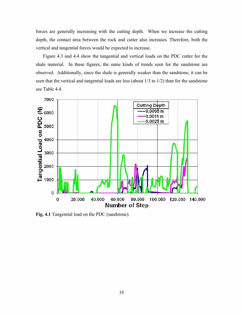
35

forces are generally increasing with the cutting depth. When we increase the cutting

depth, the contact area between the rock and cutter also increases. Therefore, both the

vertical and tangential forces would be expected to increase.

Figure 4.3 and 4.4 show the tangential and vertical loads on the PDC cutter for the

shale material. In these figures, the same kinds of trends seen for the sandstone are

observed. Additionally, since the shale is generally weaker than the sandstone, it can be

seen that the vertical and tangential loads are less (about 1/3 to 1/2) than for the sandstone

see Table 4.4.

Fig. 4.1 Tangential load on the PDC (sandstone).

36

Fig. 4.2 Vertical Load on the PDC (sandstone).

Fig. 4.3 Tangential Load on the PDC (shale).

37

Fig. 4.4 Vertical Load on the PDC (shale)

Table 4.4 shows the average tangential and vertical loads on cutter for a sandstone

and a shale for different cutting depths. When the cutting depth increased from 0.0005 m

to 0.0011 m and from 0.0011m to 0.0025 m, average cutter loads increased for both the

sandstone and the shale. When the average cutter loads for a shale and a sandstone are

compared for each individual cutting depth, cutter loads calculated for the sandstone is

always higher then loads calculated for the shale. Therefore, the UDS model appears to

be working as expected showing an increase in tangential and vertical cutter loads

associated with increasing cutting depth and rock strength.

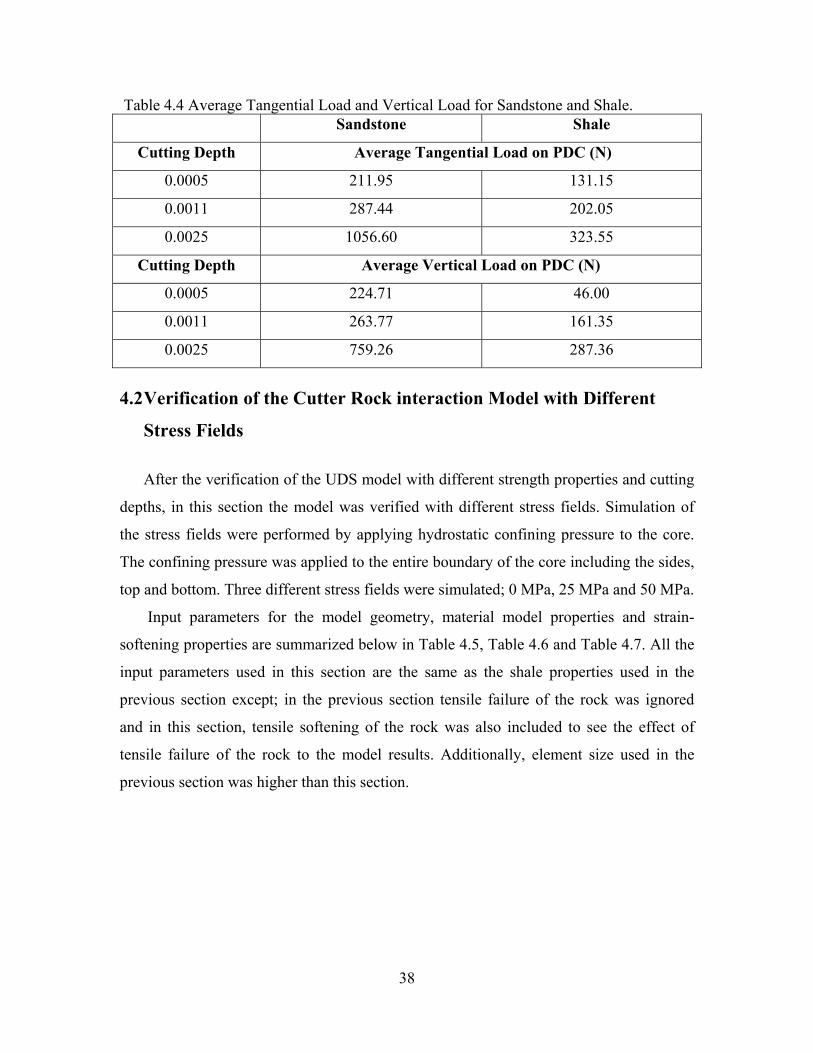
38

Table 4.4 Average Tangential Load and Vertical Load for Sandstone and Shale. Sandstone Shale

Cutting Depth Average Tangential Load on PDC (N)

0.0005 211.95 131.15

0.0011 287.44 202.05

0.0025 1056.60 323.55

Cutting Depth Average Vertical Load on PDC (N)

0.0005 224.71 46.00

0.0011 263.77 161.35

0.0025 759.26 287.36

4.2 Verification of the Cutter Rock interaction Model with Different

Stress Fields

After the verification of the UDS model with different strength properties and cutting

depths, in this section the model was verified with different stress fields. Simulation of

the stress fields were performed by applying hydrostatic confining pressure to the core.

The confining pressure was applied to the entire boundary of the core including the sides,

top and bottom. Three different stress fields were simulated; 0 MPa, 25 MPa and 50 MPa.

Input parameters for the model geometry, material model properties and strain-

softening properties are summarized below in Table 4.5, Table 4.6 and Table 4.7. All the

input parameters used in this section are the same as the shale properties used in the

previous section except; in the previous section tensile failure of the rock was ignored

and in this section, tensile softening of the rock was also included to see the effect of

tensile failure of the rock to the model results. Additionally, element size used in the

previous section was higher than this section.

39

Table 4.5 . Model geometry parameters

Core Length

(m)

Core Dia.

(m)

PDC

Thickness

(m)

PDC Dia.

(m)

Cutter Rake

Angle

Parameter

Value 0.4 0.2 0.0033 0.014 30o

Table 4.6 Material properties for the rock specimens Material Parameter

Bulk Modulus (GPa) 8.8

Shear Modulus (GPa) 4.3

Friction Angle 14.4º

Cohesion (C) (MPa) 27.2

Dilation Angle 12.0º

Tensile strength (MPa) 0.6

Table 4.7 Post-failure properties for the rock specimens.

Plastic Strain

0.00 0.05 0.10 1.00

Friction Angle 14.4º 12º 10º 10º

Cohesion (MPa) 27.2 15 1 1

Dilation Angle 12.0º 5º 0º 0º

Tensile Strength (MPa) 0.6 0 0 0

Figure 4.5 shows the resulting tangential load on the bit and Figure 4.6 shows the

resulting thrust on the bit as a function of the confining pressure. Table 4.8 summarizes

the average vertical and horizontal loads on the bit for the different stress conditions.

When confining pressure increased from 0 MPa to 25 MPa average tangential load

increased from 36.79 MPa to 56.19 MPa and average vertical load increased from 26.44

MPa to 30.97 MPa. When confining pressure increased from 25 MPa to 50 MPa average

tangential load increased from 56.19 MPa to 85.15 MPa and average vertical load

increased from 30.97 MPa to 38.79 MPa. Clearly, both the tangential and the vertical

40

loads requirements increase with increasing confining stresses, and the relationship

appears to be non-linear. Also, it can be seen that the required tangential load increases

faster than the required vertical load when confining pressure is increased. Why

tangential load increased faster than vertical load can be explained as; for these numerical

tests, the model cutting depth was set by sumping the cutter into the rock at a constant

velocity during the first 10,000 steps. After 10,000 steps the grid points at the bottom of

the core were fixed in the vertical direction, so cutting depth was fixed. Therefore, after

10,000 steps, elements were failed by the drag action of the cutter. Dynamic tangential

and vertical loads in first 10,000 steps in Figure 4.5 and 4.6 are supporting the

explanation. Dynamic cutter loads are more frequent in the first 10,000 steps.

With the changes in confining pressure, the UDS model appears to be working as

expected and shows an increase in tangential and vertical cutter loads associated with

increasing hydrostatic confining pressure. When the cutter loads those are observed in

this study are compared with the previous one (Table 4.4), these loads are lower. The

reasons of the difference are:

• In this section model element sizes were selected much smaller then the model in

the previous section. Change of the element size affected the cutter loads.

• In this section tensile softening of the rock was included in to the model. Model

results are very sensitive to tensile strength of the rock.

Table 4.8 Average horizontal and vertical loads on bit for different confining stresses

Hydrostatic Confining Stress

(MPa)

Average Tangential Load on Bit

(N)

Average Vertical Load on Bit

(N)

0 36.79 26.44

25 56.19 30.97

50 85.15 38.79

41

Fig. 4.5 Horizontal load on the bit for different confining stresses.

Fig. 4.6 Vertical load on the bit for different confining stresses.

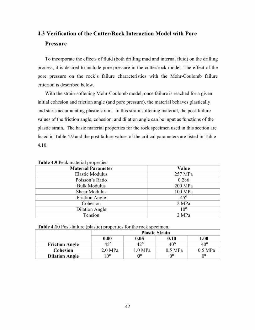
42

4.3 Verification of the Cutter/Rock Interaction Model with Pore

Pressure

To incorporate the effects of fluid (both drilling mud and internal fluid) on the drilling

process, it is desired to include pore pressure in the cutter/rock model. The effect of the

pore pressure on the rock’s failure characteristics with the Mohr-Coulomb failure

criterion is described below.

With the strain-softening Mohr-Coulomb model, once failure is reached for a given

initial cohesion and friction angle (and pore pressure), the material behaves plastically

and starts accumulating plastic strain. In this strain softening material, the post-failure

values of the friction angle, cohesion, and dilation angle can be input as functions of the

plastic strain. The basic material properties for the rock specimen used in this section are

listed in Table 4.9 and the post failure values of the critical parameters are listed in Table

4.10.

Table 4.9 Peak material properties Material Parameter Value

Elastic Modulus 257 MPa Poisson’s Ratio 0.286 Bulk Modulus 200 MPa Shear Modulus 100 MPa Friction Angle 45º

Cohesion 2 MPa Dilation Angle 10º

Tension 2 MPa Table 4.10 Post-failure (plastic) properties for the rock specimen.

Plastic Strain 0.00 0.05 0.10 1.00

Friction Angle 45º 42º 40º 40º Cohesion 2.0 MPa 1.0 MPa 0.5 MPa 0.5 MPa

Dilation Angle 10º 0º 0º 0º

43

If equation 3.3 is solved for the major principal stress at failure as a function of the

confining pressure, pore pressure and rock properties, we get:

φφ

φφ

σσ

σσ

NcNPP

NcNPP

2)(

2)()(0

31

31

+−+=

+−+−−= (4.1)

If the material properties listed in Table 4.9 and Table 4.10 are substituted into

equation 4.1 for a uni-axial compressive test, we find that the failure stress should be 9.65

MPa:

MPa

SinSinN

65.982.5102282.5)00(0

)45(1)45(1

1

61

=×××+×−+=

−+

=

σσ

φ

(4.2)

If the initial pore pressure of the rock is now assumed to be 1MPa (with the same

material properties) are we find that equation 4.1 becomes and the failure stress would

now be 4.83 MPa:

MPa83.482.5102282.5)1010()101(

1

6661

=×××+××−+×=

σσ (4.3)

To validate the hydro mechanical response of the cutter/rock model, a model with

pore pressure was developed with the material properties listed in the Table 4.9 and Table

4.10 were used in this model. In this pore pressure model, the internal pore pressure of

the rock was set at 1 MPa. The essential results from this model are shown in Figures 4.7

and 4.8 which graph the vertical and horizontal load on the cutter with and without the

pore pressure respectively. In these graphs, it is easy to see that the forces are lower with

the addition of the pore pressure, which indicates that the rock is failing much easier.

Table 4.11 summarizes the resultant average cutter loads and uni-axial compressive

strength (UCS) with pore pressure and without pore pressure. The UCS of the rock

decreased to half of its’ original value when the initial pore pressure is set to 1MPa. Also,

the average vertical load showed about the same amount of drop with 1 MPa of initial

pore pressure. This is a consistent response to the addition of the pore pressure and

44

indicates that the hydro-mechanical response of the cutter-rock model is working as

expected.

Table 4.11 Average cutter loads and uni-axial compressive strength (UCS)

Initial Pore Pressure (MPa)

Cutter/Rock Model Uni-Axial Model

Average Vertical Load (N)

Average Horizontal Load

(N) UCS (MPa)

0 408 181 9.65 1 194 115 4.83

Fig. 4.7 Comparison of the vertical load on the cutter with a change in pore pressure.

45

Fig. 4.8 Comparison of the horizontal load on the cutter with a change in pore pressure.

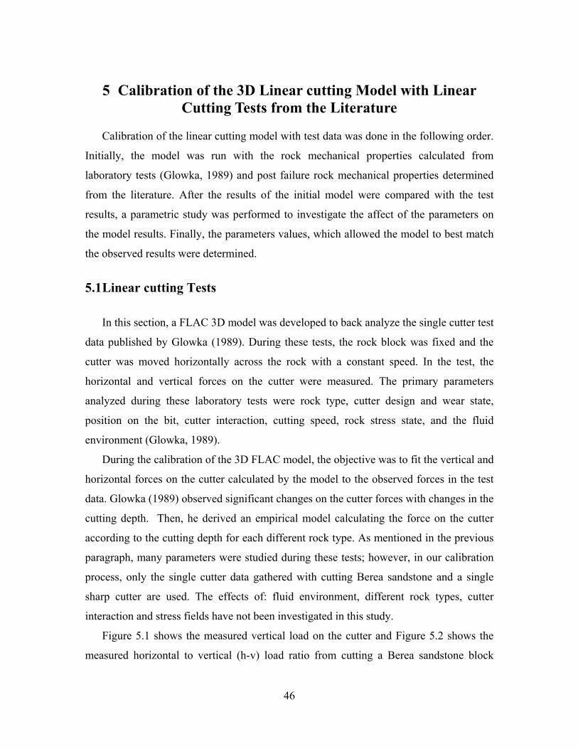
46

5 Calibration of the 3D Linear cutting Model with Linear Cutting Tests from the Literature

Calibration of the linear cutting model with test data was done in the following order.

Initially, the model was run with the rock mechanical properties calculated from

laboratory tests (Glowka, 1989) and post failure rock mechanical properties determined

from the literature. After the results of the initial model were compared with the test

results, a parametric study was performed to investigate the affect of the parameters on

the model results. Finally, the parameters values, which allowed the model to best match

the observed results were determined.

5.1 Linear cutting Tests

In this section, a FLAC 3D model was developed to back analyze the single cutter test

data published by Glowka (1989). During these tests, the rock block was fixed and the

cutter was moved horizontally across the rock with a constant speed. In the test, the

horizontal and vertical forces on the cutter were measured. The primary parameters

analyzed during these laboratory tests were rock type, cutter design and wear state,

position on the bit, cutter interaction, cutting speed, rock stress state, and the fluid

environment (Glowka, 1989).

During the calibration of the 3D FLAC model, the objective was to fit the vertical and

horizontal forces on the cutter calculated by the model to the observed forces in the test

data. Glowka (1989) observed significant changes on the cutter forces with changes in the

cutting depth. Then, he derived an empirical model calculating the force on the cutter

according to the cutting depth for each different rock type. As mentioned in the previous

paragraph, many parameters were studied during these tests; however, in our calibration

process, only the single cutter data gathered with cutting Berea sandstone and a single

sharp cutter are used. The effects of: fluid environment, different rock types, cutter

interaction and stress fields have not been investigated in this study.

Figure 5.1 shows the measured vertical load on the cutter and Figure 5.2 shows the

measured horizontal to vertical (h-v) load ratio from cutting a Berea sandstone block

47

using a 12.7 mm diameter PDC bit in the laboratory (Glowka, 1989). In the figures, it can

be seen that the vertical load increased fairly linearly and the load ratio stayed fairly

constant with the increasing depth of cut.

Fig. 5.1 Test results used for calibration of the FLAC3D model.

48

Fig. 5.2 Horizontal load over vertical load ratio for different depth of cut.

5.2 Linear Cutting Model Development

Grid generation for the linear cutting tests performed to represent the 3D geometry of

the test setup presented on the previous chapter. Fish function was developed to generate

geometry of the rock and cutter as a parametric. Therefore, cutter thickness, diameter,

grid density and rock width, length and grid density can be controlled for each model

without spending much effort. For the model, the rock specimen was generated on a

rectangular grid and the cutter was generated as a cylindrical grid. The grid design of the

rock consists of three sections in the vertical direction with consistent element sizes

within each section and with the grid density increasing towards the top of the model.

The element size changes between sections in the vertical direction were kept to a factor

of two in order to minimize stress concentrations at the section boundaries.

Figure 5.3 illustrates the boundary conditions used during single cutter model. Cutter

is fixed from the top and a constant velocity is applied to the rock specimen on the global

49

X axes direction as shown on the figure. Additionally, movement of the rock is restricted

on the X direction towards cutter.

Fig. 5.3 Illustration of the single cutter model geometry and boundary conditions.

5.3 Calibration of the 3D Linear cutting Model with Linear Cutting

Tests from the Literature

Table 5.1 shows the mechanical properties of the Berea Sandstone determined from

laboratory tests, and Table 5.2 shows the ranges of the mechanical properties ultimately

used in the FLAC3D model.

Table 5.1 Mechanical Properties of Berea Sandstone

Internal

Friction

Angle

UCS (MPa) Elastic

Modulus

(GPa)

Poissons

Ratio

Tensile

Strength

(MPa)

Max 53.6 70 16 - 4

Min 23.4 47 12 - 2

Average - 49 14 0.36 3

50

Table 5.2 Mechanical properties used in FLAC model

Internal

Friction Angle UCS (MPa)

Elastic

Modulus

(GPa)

Poissons Ratio

Tensile

Strength

(MPa)

40 - 30 50 - 60 14 0.36 15 - 45

A continuum model can simulate the propagation of a crack and the formation of the

chip, but in FLAC3D the chip does not natural interact with the rest of the continuum

geometry after it is formed. This is one drawback of using a continuum model to simulate

the cutter/rock interaction, where chipping is known to occur and may influence the

cutting loads. In the FLAC model, the propagation of a crack is observed in the model as

strain localization when the model elements are small enough and a strain softening

material model is used. As previously mentioned on Chapter 2 and 3, Stavropoulou

(2006) showed the formation of a chip with FLAC2D. However, he was only able to

model a single initial chip during the cutting process, which is not realistic. The true rock

cutting process requires the production of multiple chips as the cutter moves.

In this study, to simulate complete failure of the material and removal of the “chips”,

once a rock element reaches a pre-determine amount of plastic strain, that element is

changed to a “null” material and essentially removed from the model. This approach

allows more realistic modeling of the cutter rock interaction, and with the sporadic

element removal, the dynamic cutter loads observed during the tests can be also seen in

the model. Figure 5.4 shows the propagation of a crack and formation of a chip with the

FLAC3D model. During the initial stages of loading, the rock starts to deform (figure 5.4

(a), (b)). Then a fracture starts to propagate until the formation of the chip (figure 5.4 (c),

(d), (e), and (f)). The propagation of the crack is simulated by the failure of the element

zones according to Mohr-Coulomb criterion and the removal of the zones at a certain

predetermined percentage (30% in this case) of plastic strain.

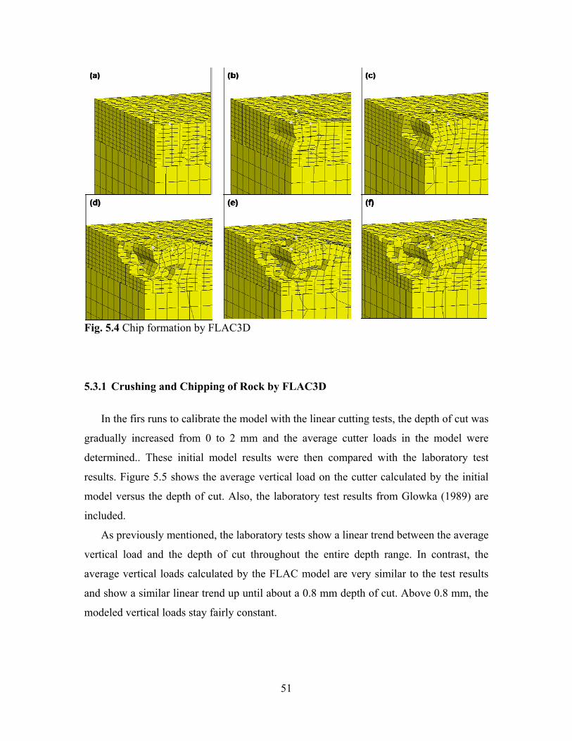
51

Fig. 5.4 Chip formation by FLAC3D

5.3.1 Crushing and Chipping of Rock by FLAC3D

In the firs runs to calibrate the model with the linear cutting tests, the depth of cut was

gradually increased from 0 to 2 mm and the average cutter loads in the model were

determined.. These initial model results were then compared with the laboratory test

results. Figure 5.5 shows the average vertical load on the cutter calculated by the initial

model versus the depth of cut. Also, the laboratory test results from Glowka (1989) are

included.

As previously mentioned, the laboratory tests show a linear trend between the average

vertical load and the depth of cut throughout the entire depth range. In contrast, the

average vertical loads calculated by the FLAC model are very similar to the test results

and show a similar linear trend up until about a 0.8 mm depth of cut. Above 0.8 mm, the

modeled vertical loads stay fairly constant.

52

Fig. 5.5 Average vertical load on cutter versus depth of cut (initial model) .

After examining the FLAC models in detail, it was determined that the reason the

modeled vertical loads increased linearly between 0 – 0.8 mm, but stay constant after

that, is a change of the failure mode of the rock elements from crushing to chipping as the

depth of cut increases. Below the 0.8 mm depth of cut, the elements primarily fail by

crushing of the zones under the cutter and shear failure is predominate. Above a 0.8 mm

cutting thickness, brittle failure and chipping of the rock is observed in the model (Figure

5.4). In the case of chipping, tension failure is predominate. This same response was

observed by Richard et al. (1998) in relation to their laboratory experiments. In that paper

(as mentioned in Chapter 2), they reported that two different failure modes take place

depending on the depth of cut, ductile or brittle. The test results published by Richard et

al. (1998) also show the cutter forces becoming fairly constant above a particular depth of

cut (Figure 2.6). Unfortunately, Glowka (1989) did not give any distinct comment on the

failure mode observed during his linear cutting tests.

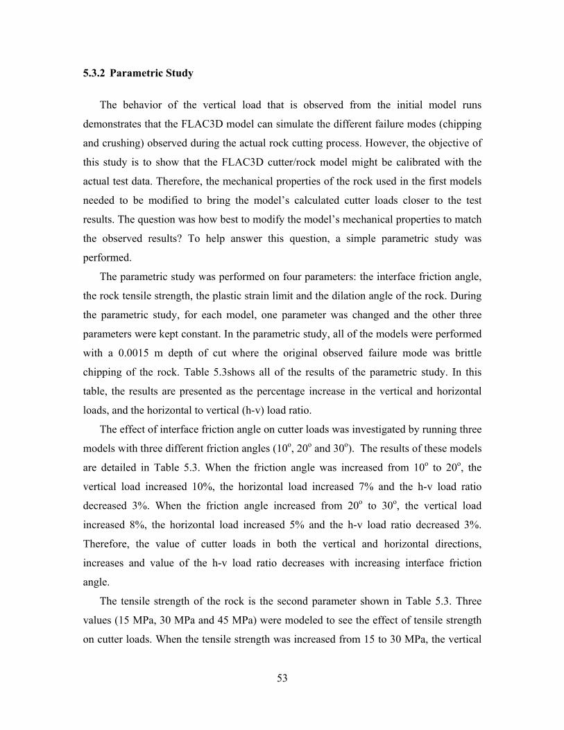
53

5.3.2 Parametric Study

The behavior of the vertical load that is observed from the initial model runs

demonstrates that the FLAC3D model can simulate the different failure modes (chipping

and crushing) observed during the actual rock cutting process. However, the objective of

this study is to show that the FLAC3D cutter/rock model might be calibrated with the

actual test data. Therefore, the mechanical properties of the rock used in the first models

needed to be modified to bring the model’s calculated cutter loads closer to the test

results. The question was how best to modify the model’s mechanical properties to match

the observed results? To help answer this question, a simple parametric study was

performed.

The parametric study was performed on four parameters: the interface friction angle,

the rock tensile strength, the plastic strain limit and the dilation angle of the rock. During

the parametric study, for each model, one parameter was changed and the other three

parameters were kept constant. In the parametric study, all of the models were performed

with a 0.0015 m depth of cut where the original observed failure mode was brittle

chipping of the rock. Table 5.3shows all of the results of the parametric study. In this

table, the results are presented as the percentage increase in the vertical and horizontal

loads, and the horizontal to vertical (h-v) load ratio.

The effect of interface friction angle on cutter loads was investigated by running three

models with three different friction angles (10o, 20o and 30o). The results of these models

are detailed in Table 5.3. When the friction angle was increased from 10o to 20o, the

vertical load increased 10%, the horizontal load increased 7% and the h-v load ratio

decreased 3%. When the friction angle increased from 20o to 30o, the vertical load

increased 8%, the horizontal load increased 5% and the h-v load ratio decreased 3%.

Therefore, the value of cutter loads in both the vertical and horizontal directions,

increases and value of the h-v load ratio decreases with increasing interface friction

angle.

The tensile strength of the rock is the second parameter shown in Table 5.3. Three

values (15 MPa, 30 MPa and 45 MPa) were modeled to see the effect of tensile strength

on cutter loads. When the tensile strength was increased from 15 to 30 MPa, the vertical

54

load increased 133%, the horizontal load increased 119% and the h-v load ratio decreased

6%. When the tensile strength was increased from 30 to 45 MPa, no significant change

was observed. The cutter loads showed a very sharp rise when the tensile strength of the

rock was increased from 15 MPa to 30 MPa because the cutting depth of the model was

set to 0.0015 m where the predominant failure mode was tensile chipping with the lower

tensile strength. Once the tensile strength of the rock was increased, the predominate

failure mode changed to shear with a corresponding increase in modeled loads.

The third parameter shown in Table 5.3 is the plastic strain limit. This is the limit of

post-failure, plastic strain where the elements are “nulled” and removed from the model.

Two values of plastic strain limits were tested, 15% and 35%. When the strain limit was

increased from 15% to 35%, the vertical load increased 23%, the horizontal load

increased 8% and h-v load ratio decreased 14%.

The last parameter to be investigated in Table 5.3 is the dilation angle. The dilation

angle controls the volume increase, or expansion, of the material due to failure, and the

dilatancy of the material increases with increasing dilation angle. For the sensitivity

study, four values of dilation angle were tested (0°, 5°, 10° and 15°). When the dilation

angle was increased from 0° to 5°, the vertical load increased 13%, the horizontal load

increased 6% and h-v load ratio decreased 6%. When the dilation angle was increased

from 5° to 10°, vertical load increased 12%, horizontal load increased 3% and the load

ratio decreased 8%. When the dilation angle was increased from 10° to 15°, the vertical

load increased 19%, the horizontal load increased 9% and the h-v load ratio decreased

9%. These results show that the materials with the higher dilation angles essentially

behave stiffer and show a higher resistance to the loading.

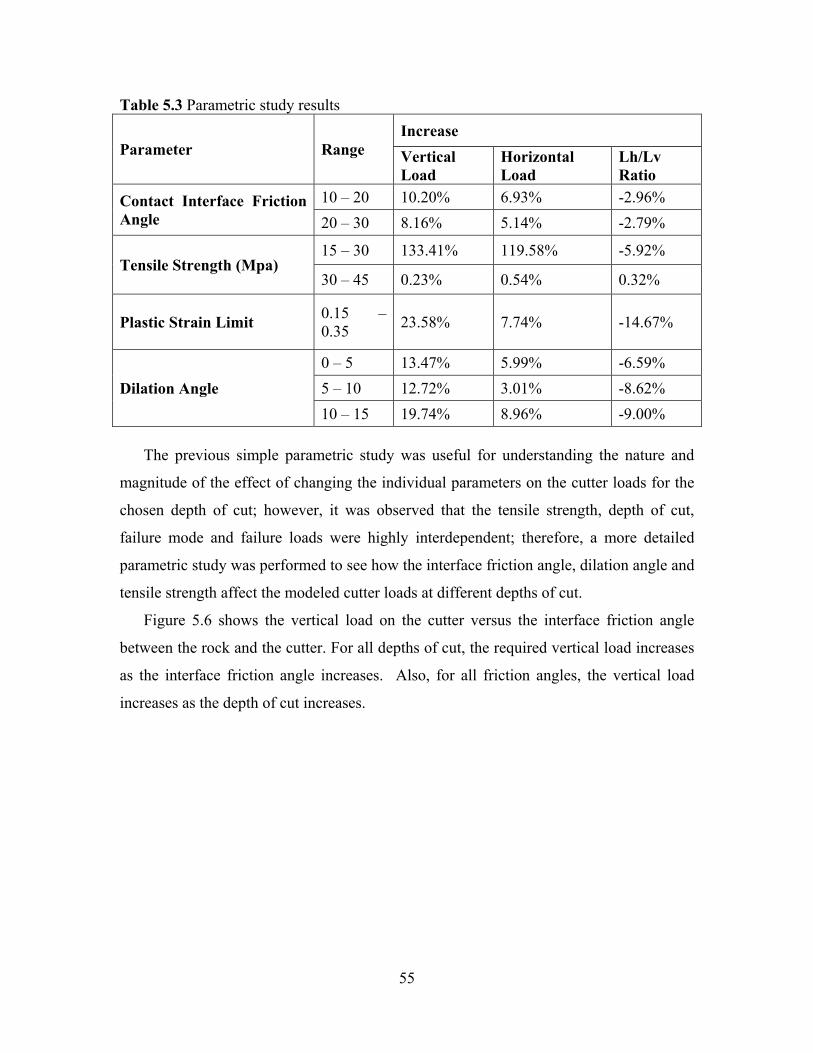
55

Table 5.3 Parametric study results

Parameter Range Increase Vertical Load

Horizontal Load

Lh/Lv Ratio

Contact Interface Friction Angle

10 – 20 10.20% 6.93% -2.96% 20 – 30 8.16% 5.14% -2.79%

Tensile Strength (Mpa) 15 – 30 133.41% 119.58% -5.92%

30 – 45 0.23% 0.54% 0.32%

Plastic Strain Limit 0.15 – 0.35 23.58% 7.74% -14.67%

Dilation Angle 0 – 5 13.47% 5.99% -6.59% 5 – 10 12.72% 3.01% -8.62% 10 – 15 19.74% 8.96% -9.00%

The previous simple parametric study was useful for understanding the nature and

magnitude of the effect of changing the individual parameters on the cutter loads for the

chosen depth of cut; however, it was observed that the tensile strength, depth of cut,

failure mode and failure loads were highly interdependent; therefore, a more detailed

parametric study was performed to see how the interface friction angle, dilation angle and

tensile strength affect the modeled cutter loads at different depths of cut.

Figure 5.6 shows the vertical load on the cutter versus the interface friction angle

between the rock and the cutter. For all depths of cut, the required vertical load increases

as the interface friction angle increases. Also, for all friction angles, the vertical load

increases as the depth of cut increases.

56

Fig. 5.6 Vertical load versus interface friction angle at various depths of cut.

Figure 5.7 shows the horizontal load on the cutter versus the interface friction angle

between the rock and the cutter. The horizontal load shows the same trend the vertical

load follows. For all depths of cut, the required horizontal load increases as the interface

friction angle increases or as the depth of cut increases. However, the increase in the

horizontal load is seen to lessen as the depth of cut increases.

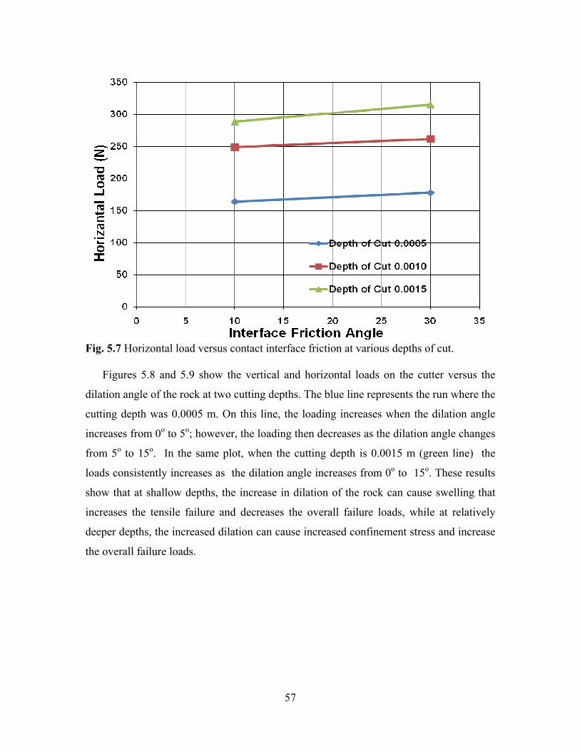
57

Fig. 5.7 Horizontal load versus contact interface friction at various depths of cut.

Figures 5.8 and 5.9 show the vertical and horizontal loads on the cutter versus the

dilation angle of the rock at two cutting depths. The blue line represents the run where the

cutting depth was 0.0005 m. On this line, the loading increases when the dilation angle

increases from 0o to 5o; however, the loading then decreases as the dilation angle changes

from 5o to 15o. In the same plot, when the cutting depth is 0.0015 m (green line) the

loads consistently increases as the dilation angle increases from 0o to 15o. These results

show that at shallow depths, the increase in dilation of the rock can cause swelling that

increases the tensile failure and decreases the overall failure loads, while at relatively

deeper depths, the increased dilation can cause increased confinement stress and increase

the overall failure loads.

58

Fig. 5.8 Vertical load versus dilation angle at various depths of cut.

Fig. 5.9 Horizontal load versus dilation angle at various depths of cut.

59

Figures 5.10 and 5.11 show the vertical and horizontal loads on the cutter versus the

depth of cut for tensile strengths of 25, 30 and 45 MPa. The blue lines show the run

where the tensile strength of the rock was equal to 15 MPa. On this line, the vertical load

decreased as the depth of cut increased from 0.0005 m to 0.0010 m, then the vertical load

essentially stayed constant when the depth of cut changed from 0.0010 m to 0.0015 m.

The red and green lines in Figures 5.10 and 5.11 show the runs with rock tensile strengths

of 30 and 45 MPa. On these lines, the vertical load increases as the depth of cut changes

from 0.0005 m to 0.0015 m.

Fig. 5.10 Vertical load versus depth of cut for tensile strengths: 15MPa, 30MPa and

45MPa.

These results demonstrate how at shallow depths of cut (0.0005 m), crushing failure

predominates and the increase in tensile strength does not greatly increase the failure

loads. However, at greater depths of cut (0.0010 and 0.0015 m), if the tensile strength is

low, then tensile failure (chipping) predominates and the cutting loads are low, but if the

tensile strength is high, then shear failure (crushing) predominates and the cutting loads

are high and not greatly affected by a small change in tensile strength.

60

Fig. 5.11 Horizontal load versus depth of cut for tensile strengths: 15MPa, 30MPa and

45MPa.

5.3.3 CALIBRATION OF THE 3D MODEL

After the parametric study was completed and a better understanding of the specific

effect of the various model input parameters was gained, the linear cutter rock model was

“calibrated” to better match the observed laboratory results. For this calibration, the

tensile strength of the rock was increased to 30 MPa, the interface friction angle was set

to 30° and the dilation angle of the rock was set to 10° and post failure input parameters

were set in to the model as listed in Table 5.4.

Table 5.4 Post failure properties used in the final FLAC model.

Plastic Strain 0.00 0.01 0.05 1.00

Friction Angle 30º 28º 28º 28º Cohesion (MPa) 18 10 5 5 Dilation Angle 10º 10º 10º 10º

61

Figure 5.12 shows the vertical load versus the depth of cut for both the calibrated

model results and the laboratory test results. In this plot, there is fairly good agreement

between the model and the lab tests. When the depth of cut was less than 0.0010 m, the

vertical load calculated by the model was generally a little higher than the test results and

when depth of cut was higher than 0.0010 m, the model calculated the vertical loads a

little less than the test results. The reason the model exhibits this behavior is that the

failure mode is still transitioning to tensile failure at greater depths of cut and somewhat

reducing the failure loads.

Fig. 5.12 Vertical load versus depth of cut (calibrated model).

Figure 5.13 shows the horizontal load over vertical load ratio calculated by model for

different depths of cut and test results. Until the 0.001 m depth of cut, model results are

very close to the test data, but after the 1 mm model predicts load ratio lower than the test

data. Additionally, the load ratio shows a decreasing trend with increasing depth of cut.

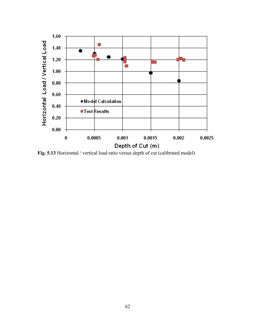
62

Fig. 5.13 Horizontal / vertical load ratio versus depth of cut (calibrated model)

63

6 Summary and Conclusions

Economical extraction of oil and gas reserves under deep formations is important for

the future energy needs of the USA. However, oil and gas production from deep

formations has challenging drilling environments. Rock hardness and abrasiveness

generally increase as the depth increase. High temperature and high pressure at this depth

along with the harder rock increase bit wear and shorten the bit life. Optimizing the

drilling performance in these HPHT operations is very important to successful, economic

mineral extraction.

DOE is searching for a cutter/rock interaction model which will be used to support

the UDS and to back analyze the experiments in the UDS. The cutter-rock model,

coupled with the UDS experiments, might then be used to analyze the influence of:

temperature, pressure, formation and mud properties, bit design and drilling parameters

on the cutting process and ultimately optimize drilling rate of penetration in HPHT

conditions.

Previous numerical models in the literature helped to identify some important aspects

of the drilling environment. However, only a few of them were validated with laboratory

data and the intent was never to calibrate the model with reality. Additionally, these

models were two dimensional; and therefore, they were not representative of the actual

3D geometry of the UDS or the field.

A cutter/rock interaction model which will be used to optimize drilling operations

should be capable of simulating the true three dimensional geometry and boundary

conditions of the UDS. Also, it should calculate cutter loads close to the actual field or

test data. Also, bottom-hole stresses, pore fluid pressure, overburden pressure, mud

pressure and differential pressure and material behavior when subjected to these factors,

needs to be modeled correctly.

Therefore, goal of this thesis is to develop a three dimensional numerical model of a

single cutter interacting with the rock formation to simulated the Ultra Deep Drilling

Simulator (UDS) and model with the true 3D geometry of UDS sample simulation.

Initially, the model is demonstrated to show that it can reasonably simulate the UDS

experiments with different rock formations, stress environments and fluid pressures.

64

Additionally, a linear cutter model (very similar to the UDS model) is calibrated with

single cutter test data published in the literature to investigate the difficulty of calibrating

the model and the degree of fit that can be obtained between the numerical model and the

laboratory tests.

For the UDS model, a parametric FLAC3D model geometry was developed so that

the cutter size, cutter angle, cutter thickness, cutter location, rock specimen size,

specimen length and the element sizes can be easily changed from one test geometry to

the next. The interface between the cutter and the rock specimen was generated with a

“soft” contact formulation where the interface elements are allowed to interpenetrate the

contact target face. The interface has the properties of Coulomb sliding with: friction

angle, normal and shear stiffnesses.

The boundary or loading conditions on the model are developed to get exactly match

the UDS loading conditions. For the axial load (or thrust) on the rock specimen, a

constant velocity is applied to the bottom of the core in the vertical direction. In order to

rotate the core, a constant linear velocity is applied to the nodes on the outer edge of the

bottom of the core, and the center nodes of the core are fixed in the horizontal directions.

Accurate calculation of the rock failure behavior in the model is critical to accurately

modeling the behavior of the entire cutter-rock system. In this study, the cutter-rock

model uses the strain-softening Mohr-Coulomb plasticity material. With the strain-

softening Mohr-Coulomb model, once failure is reached for a given initial cohesion and

friction angle (and pore pressure), the material behaves plastically and starts to

accumulate plastic strain. This modeling approach is developed to simulate complete

failure of the material and removal of the “chips”, once the rock material reaches a pre-

determine amount of plastic strain at a given element, that element is changed to a “null”

material and essentially removed from the model. This approach allowed us to model

cutter rock interaction more realistically. Moreover, it also allows us to observe dynamic

cutter loads in the model as observed in practice.

The initial runs of the FLAC3D model are used to investigate two different rock types

(a sandstone and a shale) with three different cutting depths (penetration rates). The first

thing observed from the model results are; dynamic cutter loads seen on the practice was

also seen on the model calculations. When the thrusts and torques for different cutting

65

depths are compared, it can be clearly seen that the forces are generally increasing with

the cutting depth for both rock types. When we increase the cutting depth, the contact

area between the rock and cutter also increases. Therefore, both the vertical and

tangential forces would be expected to increase. Additionally, since the shale is generally

weaker than the sandstone, it can be seen that the vertical and tangential loads are less

(about 1/3 to 1/2) than for the sandstone see (Table 4.4)

The effect of various confining stress levels on the single cutter tests are analyzed by

applying three different hydrostatic confinements. In this analysis, both the torque and the

thrust requirements increase with increase in confining stresses, and the relationship

appears to be non-linear (Table 4.8).

In order to investigate the effect of the pore pressure to the cutter/rock model, initially

a model is run with 1 MPA and 0 MPa initial pore pressures. When results of the zero

initial pore pressure and 1MPa initial pore pressure models compared, forces are lower

with the addition of the pore pressure, which indicates that the rock is failing much easier

(Table 4.11). This is a consistent response to the addition of the pore pressure and

indicates that the hydro-mechanical response of the cutter-rock model is working

properly.

Ultimately, A FLAC 3D model was developed to back analyze the single cutter test

data published by Glowka (1989). During the calibration of the 3D FLAC model, the

objective was to fit the vertical and horizontal forces on the cutter calculated by the

model to the observed forces in the test data. The model eventually calculated the cutter

loads pretty close to the test results. It was found that the different failure modes in the

cutter/rock model, shear (crushing) and tensile (chipping), are highly dependent on the

depth of cut and the tensile strength of the rock and greatly affect the cutting loads. Also,

it was found that the model failure process (strain localization) is known to be grid size

dependent; therefore, different grid sizes may change the results.

As a conclusion, three dimensional FLAC model of a single cutter interacting with

the rock formation of UDS was validated with different rock formations, stress

environments and fluid pressures. Additionally, a linear cutter model was calibrated with

single cutter test data published in the literature. Model predictions were close to actual

test data.

66

Following future research can be carried out to get more accurate cutter/rock model:

1. Different failure criterions may be used to seek more accurate prediction of cutter

loads.

2. The model results are known to be grid size dependent; therefore, different grid

sizes will change the results. A rate independent, non-local failure criterion, which

would be implemented into FLAC, might solve this problem.

3. Mechanically coupled pore pressure can be used in the analysis to include the

local pore pressure effect on the model.

67

REFERENCES

1) Abd AL-Jalil, Y. Q., 2006, “The Mechanics of Indentation of Rock - A Critical

Review”, Proceedings of the 41st U.S. Symp. On Rock Mechanics, Golden, CO,

June 17-21, Paper 06- 1082, 18 p.

2) Bruno, M., G. Han and C. Honeger, 2005, “Advanced Simulation Technology for

Combined Percussion and Rotary Drilling and Cuttings transport, GasTIPS, 5-8.

3) Energy Information Administration, “Energy Information Administration Annual

Review 2007” (2008)

4) Feenstra R., “Status of Polycrystalline-Diamond-Compact Bits: Part 1-

Development” JPT, June, (1988), pp. 677 - 684

5) Feenstra R. “New Generation of Oilfield Bits – Laboratory and Field Results”

paper SPE 6712 presented at the SPE Annual Technical Conference and

Exhibition, Denver, Oct. 9 – 12, (1977)

6) Glowka D. A., “Use of Single-Cutter Data in the Analysis of PDC Bit Designs:

Part 1- Development of a PDC Cutting Force Model” JPT, August, (1989), pp.

797 –

7) Glowka D. A., “Use of Single-Cutter Data in the Analysis of PDC Bit Designs:

Part 2- Development and Use of the PDCWEAR Computer Code” JPT, August,

(1989), pp. 797 –

8) Han, G., M. Bruno, and T. Grant, 2006, “Lab Investigations of Percussion

Drilling: From Single Impact to Full Scale Fluid Hammer,” Proceedings of the

41st U.S. Symposium on Rock Mechanics, Golden, CO, June 17-21, Paper 06-

962.

9) Han, G., M. Bruno, and M. B. Dusseault, 2005, “Dynamic Modeling Rock Failure

in Percussion Drilling,” Proceedings of the 40th U.S. Symposium on Rock

Mechanics, Anchorage, AK, June 25-29, Paper 05-819, 7 p.

68

10) Huang. H, E. Detournay, and B. Bellier. 1999. Dicrete Element Modeling of Rock

Cutting. In Proceedings of 37th US Rock Mechanics Symposium, Vail, CO, June 6

– 9, 1999

11) Itasca Consulting Group, Inc., 2007. FLAC3D: Theory and Background.

Minnesota, USA

12) Kou S., Some Basic Problems in Rock Breakage by Blasting and by Indentation.

Doctoral Thesis 1995:180 D, University of Lulea.

13) Kou S., Ye D. and Ding Y. “A Constitutive Model for Structured Coal Based on

Fracture and Damage Mechanics.” Engineering Fracture Mechanics, (1990), 35,

4/5, pp. 835-843

14) Leelasukseree, C., D. S. Kieffer and G. G. W.Mustoe, 2006, “Numerical

Simulation of Disc Cutter Behavior in Bimrocks,” Proceedings of the 41st U.S.

Symposium on Rock Mechanics, Golden, CO, June 17-21, Paper 06-1146.

15) Lyons K. D., Honeygan S. and Mroz T. “NETL Extreme Drilling Laboratory

Studies High Pressure High Temperature Drilling Phenomena” Proceedings of

26th International Conference on Offshore Mechanics and Artic Engineering

OMEA2007, San Diego, CA, June 10 -15., (2007)

16) Maurer W. C. “Shear Failure of Rock Under Compression” Society of Petroleum

Engineering Journal, June, (1965), pp. 167-176

17) Maurer W. C., “Bit Tooth Penetration Under Simulated Borehole Conditions”,

JPT, Trans., AIME, Dec., (1965), pp.1433 – 1442

18) Richard T., Detournay E., Drescher A., Nicodeme P. and Fourmaintraux D., “ The

Scratch Test a Means to Measure Strength of Sedimentary Rocks” SPE/ISRM

Eurock 98, Trondheim, Norway, 8-10 July, (1998) pp. 15 -22

19) Saouma, V.E. and M. Kleinosky, 1984, “Finite Element Simulation of Rock

Cutting: A Fracture Mechanics Approach,” Proceedings of the 25th U.S.

Symposium on Rock Mech., ASCE, p. 792.

69

20) Stavropoulou, M. 2006. Modeling of Small-Diameter Rotary Drilling Tests on

Marbles. Int. J. of Rock Mech. Min. Sci. 43, 1.34 – 1051.

21) Terzaghi K. and Peck R. B., Soil Mechanics in Engineering Practice , John Wiley

& Sons, Inc., NY, (1948) pp. 566

22) U.S. Geological Survey (USGS) National Oil and Gas Resource Assessment

Team, :”1995 National Assessment of United States Oil and Gas Resources.” U.S.

Geological Survey Circular 1118 (1995)

23) Vermeer, P. A., and R. de Borst. “Non-Associated Plasticity for Soils, Concrete

and Rock,” Heron, 29(3), 3-64, 1984.

24) Warren T. M. and Smith M. B., “Bottomhole Stress Factors Affecting Drilling

Rate at Depth”, JPT, August, (1985), pp. 1523 – 1533

25) Warren T. M. and Armagost W. K., “Laboratory Drilling Performance of PDC

Bits”, SPE Drilling Engineering, June, (1988), pp. 125 – 135

26) Warren T. M. and Sinor A., “Drill Bit Performance Modeling”, SPE Drilling

Engineering, June, (1989), pp. 119 – 127

27) Zhang, J. and J. C. Roegiers, 2005, “Poroelastic Analysis of Rock Indentation

Failure by a Drill Bit,” Proceedings of the 40th U.S. Symposium on Rock

Mechanics, Anchorage, AK, June 25-29, Paper 05-670, 5 p.