Modeling – Part of Control Design Process Fall ME451 - GGZ Week 3-4: Modeling Physical Systems...
78
2009 Fall ME451 - GGZ Page 1 Week 3-4: Modeling Physical Systems Derive mathematical models for • Electrical systems • Mechanical systems • Electromechanical system Modeling Modeling – – Part of Control Design Process Part of Control Design Process 1. Modeling Mathematical model Mathematical model 2. Analysis Controller Controller 3. Design/Synthesis 4. Implementation Plant Plant Output Output Actuator Actuator Controller Controller Sensor Sensor Input Input Electrical Systems: • Kirchhoff’s voltage & current laws Mechanical systems: • Newton’s laws
Transcript of Modeling – Part of Control Design Process Fall ME451 - GGZ Week 3-4: Modeling Physical Systems...

2009 Fall ME451 - GGZ Page 1Week 3-4: Modeling Physical Systems
Derive mathematical models for
• Electrical systems
• Mechanical systems
• Electromechanical system
Modeling Modeling –– Part of Control Design ProcessPart of Control Design Process
1. Modeling
Mathematical modelMathematical model
2. Analysis
ControllerController
3. Design/Synthesis
4. Implementation
PlantPlantOutputOutput
ActuatorActuatorControllerController
SensorSensor
InputInput
Electrical Systems:
• Kirchhoff’s voltage & current laws
Mechanical systems:
• Newton’s laws

2009 Fall ME451 - GGZ Page 2Week 3-4: Modeling Physical Systems
Modeling Physical Systems Modeling Physical Systems -- OverviewOverview
• Mathematical model is used to represent the input-output
(signal) relation of a physical system
• A model is used for the analysis, design and
simulation validation of control systems.
Physical Physical
systemsystem
ModelModel
ModelingModeling
InputInput OutputOutput
Transfer function obtained Transfer function obtained
via physical lawsvia physical laws
2009 Fall ME451 - GGZ Page 3Week 3-4: Modeling Physical Systems
Modeling Modeling –– RemarksRemarks
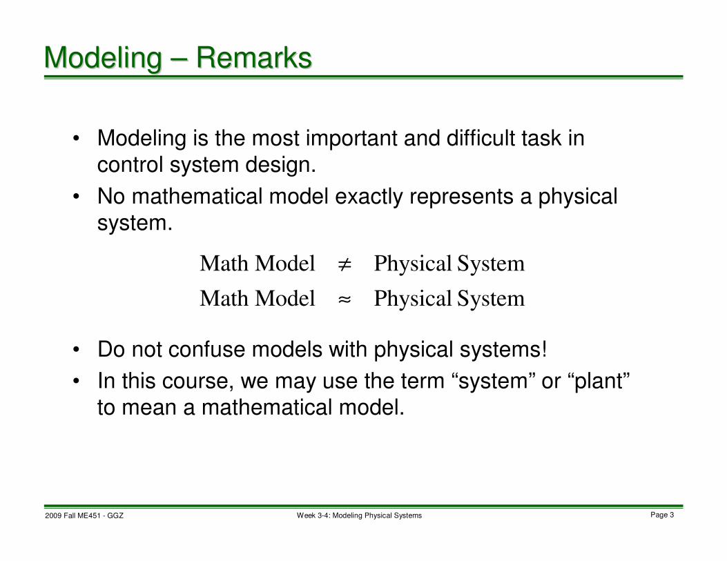
• Modeling is the most important and difficult task in
control system design.
• No mathematical model exactly represents a physical
system.
• Do not confuse models with physical systems!
• In this course, we may use the term “system” or “plant”
to mean a mathematical model.
System Physical ModelMath
System Physical ModelMath
≈
≠

2009 Fall ME451 - GGZ Page 4Week 3-4: Modeling Physical Systems
Modeling Modeling –– Transfer FunctionTransfer Function
• A transfer function is defined by
• A system is assumed to be at rest. (Zero initial condition)
Laplace transform Laplace transform
of system outputof system output
Laplace transform Laplace transform
of system inputof system input
)(
)(:)(
sU
sYsG =
)(sU )(sY)(sG
2009 Fall ME451 - GGZ Page 5Week 3-4: Modeling Physical Systems
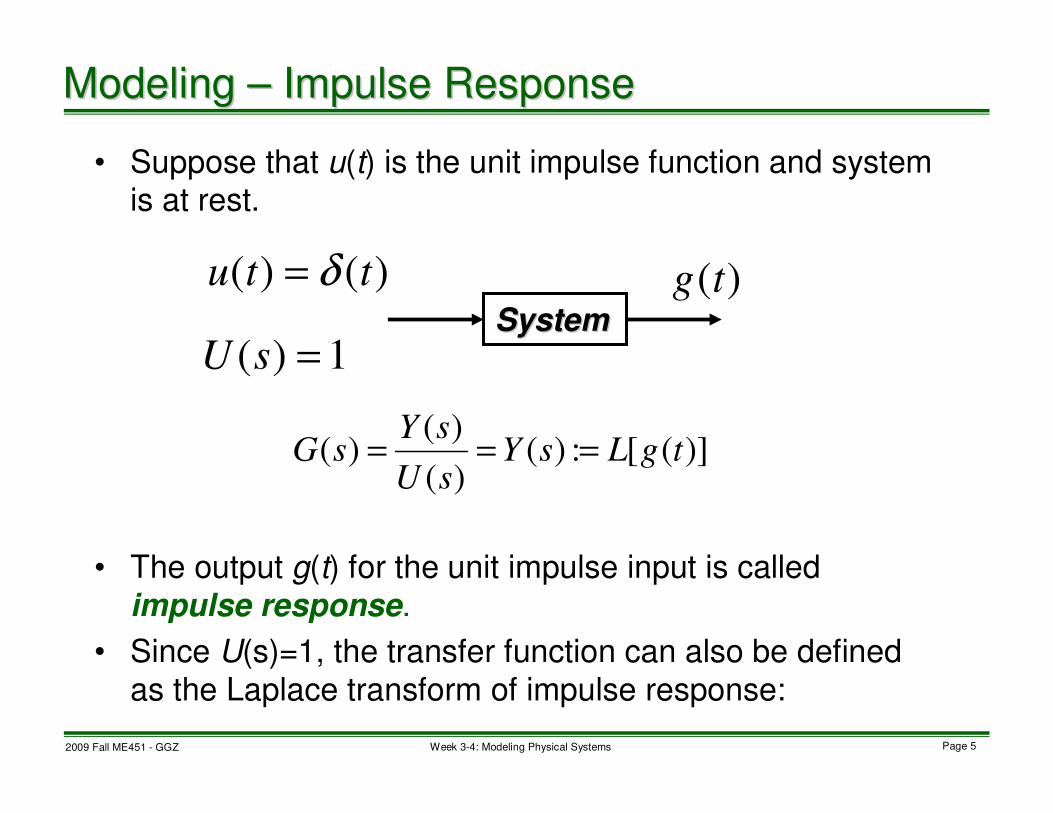
Modeling Modeling –– Impulse ResponseImpulse Response
• Suppose that u(t) is the unit impulse function and system is at rest.
• The output g(t) for the unit impulse input is called
impulse response.
• Since U(s)=1, the transfer function can also be defined
as the Laplace transform of impulse response:
SystemSystem
)]([:)()(
)()( tgLsY
sU
sYsG ===
)(tg
1)( =sU
)()( ttu δ=
2009 Fall ME451 - GGZ Page 6Week 3-4: Modeling Physical Systems
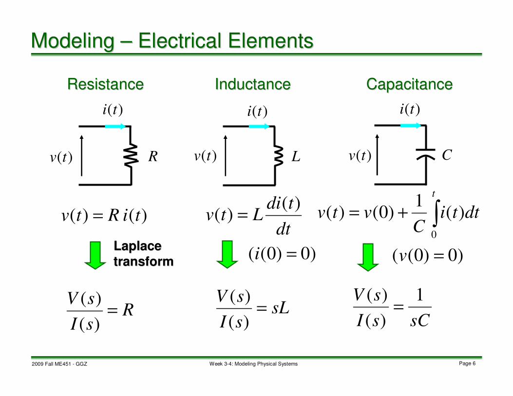
Modeling Modeling –– Electrical ElementsElectrical Elements
ResistanceResistance CapacitanceCapacitanceInductanceInductance
Laplace Laplace
transformtransform
)(ti )(ti )(ti
)(tv )(tv )(tvR L C
)( )( tiRtv =
RsI
sV=
)(
)(
dt
tdiLtv
)()( =
)0)0(( =i
sLsI
sV=
)(
)(
∫+=
t
dttiC
vtv0
)(1
)0()(
sCsI
sV 1
)(
)(=
)0)0(( =v

2009 Fall ME451 - GGZ Page 7Week 3-4: Modeling Physical Systems
Modeling Modeling –– ImpedanceImpedance
Capacitor
Inductor
Resistance
Impedances – domaint – domainElement
)resistance effective - )(( )( )()( domain,-s In sZsIsZsV =
)(sZ)(sI )(sV
)()( tRitv =
dt
tdiLtv
)()( =
∫=
t
diC
tv0
)(1
)( ττ
)()( sRIsV =
)( )( sIsLsV =
)(1
)( sIsC
sV =
R
sL
sC
1
L++= )()()( :eries in Impedance 21 sZsZsZs eff
L++=)(
1
)(
1)( :aralell in Impedance
21 sZsZsZp eff

2009 Fall ME451 - GGZ Page 8Week 3-4: Modeling Physical Systems
Modeling Modeling –– KirchhoffKirchhoff’’s Voltage & Current Lawss Voltage & Current Laws
R
LC
Sv CvRv
Ri Ci
Li
• The algebraic sum of voltage drops around any loop is zero.
• The algebraic sum of currents into any junction is zero.
Zero sum voltage:
0=++− CRS vvv
0=++− LRS vvv
Zero junction current:
0=−−LCR
iii

2009 Fall ME451 - GGZ Page 9Week 3-4: Modeling Physical Systems
Modeling Modeling –– Electrical Example 1Electrical Example 1
∫++=
t
i diC
tiRRv0
21 )(1
)()( ττ
Kirchhoff voltage law (zero
initial conditions):
1R
C
iv ovRv
i
2R
∫+=
t
o diC
tiRv0
2 )(1
)( ττ
Transfer Function
)(1
)()()( 21 sIsC
sIRRsVi ++= )(1
)()( 2 sIsC
sIRsVo +=
Laplace Transformation
CsRR
CsR
sIsC
sIRR
sIsC
sIR
sV
sVsG
i
o
)(1
1
)(1
)()(
)(1
)(
)(
)()(
21
2
21
2
++
+=
++
+
==

2009 Fall ME451 - GGZ Page 10Week 3-4: Modeling Physical Systems
Modeling Modeling –– Electrical Example 1 (contElectrical Example 1 (cont’’d)d)
Kirchhoff voltage law in frequency domain (zero initial
conditions) or impedance approach:
1R
Cs
1iv ov
Rv
)(sI
2R
Transfer Function
)(1
)()()( 21 sIsC
sIRRsVi ++= )(1
)()( 2 sIsC
sIRsVo +=
CsRR
CsR
sIsC
sIRR
sIsC
sIR
sV
sVsG
i
o
)(1
1
)(1
)()(
)(1
)(
)(
)()(
21
2
21
2
++
+=
++
+
==

2009 Fall ME451 - GGZ Page 11Week 3-4: Modeling Physical Systems
Modeling Modeling –– Electrical Example 2 (OP Amp)Electrical Example 2 (OP Amp)
Transfer Function
)()()( sIsZsV iii = )()()( sIsZsV ooo =
)(
)(
)()(
)()(
)(
)()(
sZ
sZ
sIsZ
sIsZ
sV
sVsG
i
o
ii
oo
i
o −===
--
++ )(sVo
)(sIo
)(sZo
)(sZ i)(sV
d
)(sId)(sIi
)(sVi
OP Amp Assumptions:
Infinity gain: 0)( =sVd
Infinity input impedance:
0)( =sId
)()( sIsI oi −=
2009 Fall ME451 - GGZ Page 12Week 3-4: Modeling Physical Systems
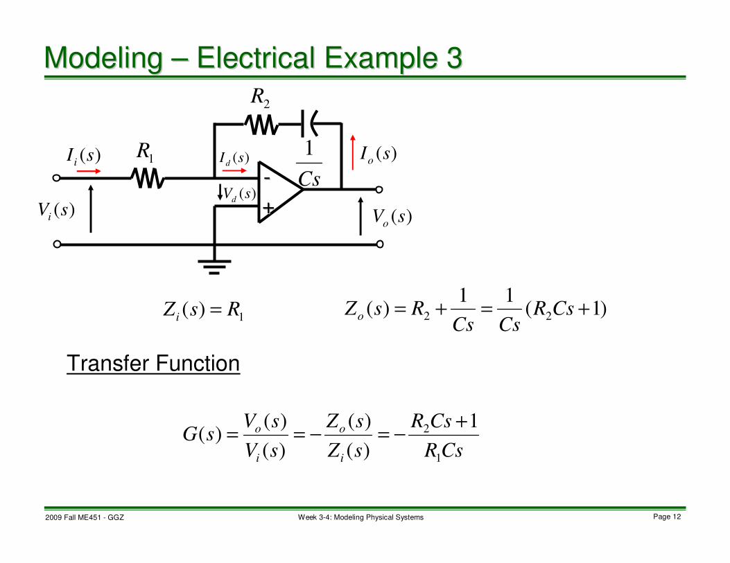
Modeling Modeling –– Electrical Example 3Electrical Example 3
Transfer Function
1)( RsZ i = )1(11
)( 22 +=+= CsRCsCs
RsZo
CsR
CsR
sZ
sZ
sV
sVsG
i
o
i
o
1
2 1
)(
)(
)(
)()(
+−=−==
--
++ )(sVo
)(sIo
)(sVd
)(sId)(sIi
)(sVi
Cs
1
2R
1R

2009 Fall ME451 - GGZ Page 13Week 3-4: Modeling Physical Systems
Modeling Modeling –– Electrical Example 4Electrical Example 4
Transfer Function
1
11
1
1
11
)(
1
R
sCRsC
RsZi
+=+=
2
221
)(
1
R
sCR
sZo
+=
1
1
)(
)(
)(
)()(
22
11
1
2
+
+⋅−=−==
sCR
sCR
R
R
sZ
sZ
sV
sVsG
i
o
i
o
--
++ )(sVo
)(sIo
)(sVd
)(sId)(sI i
)(sVi
sC2
1
2R
1R
sC1
1
2009 Fall ME451 - GGZ Page 14Week 3-4: Modeling Physical Systems
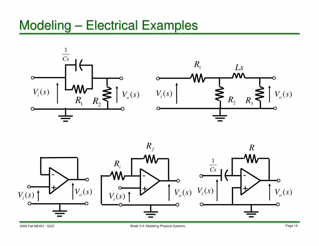
Modeling Modeling –– Electrical ExamplesElectrical Examples
)(sVo)(sVi
2R1R
Cs
1
--
++)(sVo)(sVi
--
++ )(sVo)(sVi
--
++ )(sVo)(sVi
RfR
iRCs
1
)(sVo)(sVi
3R2R
1R Ls

2009 Fall ME451 - GGZ Page 15Week 3-4: Modeling Physical Systems
Modeling Modeling –– Summary (Electrical System) Summary (Electrical System)
• Modeling
– Modeling is an important task!
– Mathematical model
– Transfer function
– Modeling of electrical systems
• Next, modeling of mechanical systems

2009 Fall ME451 - GGZ Page 16Week 3-4: Modeling Physical Systems
Modeling Modeling –– Time invariant and varying systemsTime invariant and varying systems
• A system is called time-invariant (time-varying) if system
parameters do not (do) change in time.
• Example:
• For time-invariant systems:
• This course deals with time-invariant systems.
)()()( and )()( tftxtMtftxM == &&&&
SystemSystemTime shiftTime shift Time shiftTime shift

2009 Fall ME451 - GGZ Page 17Week 3-4: Modeling Physical Systems
MassMass DamperDamperSpringSpring
M KK BB
Modeling Modeling –– Mechanical ElementsMechanical Elements
)(tf )(tx
)( )( txMtf &&=
0)0(
0)0(
=
=
x
x
&
)()( 2sXMssF =
)(tx)(tf )(tx)(tf
)( )( txKtf =
)()( sKXsF =
)( )( txBtf &=
0)0( =x
)()( sBsXsF =

2009 Fall ME451 - GGZ Page 18Week 3-4: Modeling Physical Systems
M
KK BB
Modeling Modeling –– SpringSpring--MassMass--Damper SystemsDamper Systems
)(tf )(tx
)()()()( tftKxtxBtxM =++ &&&

2009 Fall ME451 - GGZ Page 19Week 3-4: Modeling Physical Systems
M
KK BB
Modeling Modeling –– Free Body DiagramFree Body Diagram
)(tfK )(tfB )(tfK
)()( tKxtfK = )()( txBtfB&=
)(tx )(tf
)(tfB
)(tx
xMF
tx
&& :Law sNewton' Using
position resting springfor changent displaceme therepresents )( :Note
=
)()()()()()()( txBtKxtftftftftxMBK
&&& −−=−−=
)()()()( tftxBtKxtxM =++ &&&

2009 Fall ME451 - GGZ Page 20Week 3-4: Modeling Physical Systems
• Equation of motion
• By Laplace transform (with zero initial conditions),
M
KK BB
(2(2ndnd order system)order system)
Modeling Modeling –– SpringSpring--MassMass--Damper System (contDamper System (cont’’d)d)
)(tf )(tx
)()()()( tftKxtxBtxM =++ &&&
)(1
)(2
sFKBsMs
sX++
=

2009 Fall ME451 - GGZ Page 21Week 3-4: Modeling Physical Systems
M2
KK11 BB
KK22
M1Vehicle BodyVehicle Body
suspensionsuspension
wheelwheel
tiretire
Modeling Modeling –– Automotive Suspension SystemAutomotive Suspension System
)(tf
)(1 tx
)(2 tx
)())()(())()(()()(
))()(())()(()(
221211222
2112111
txKtxtxKtxtxBtftxM
txtxKtxtxBtxM
−−−−−=
−−−−=
&&&&
&&&&

2009 Fall ME451 - GGZ Page 22Week 3-4: Modeling Physical Systems
Laplace transform with zero ICsLaplace transform with zero ICs
G2 G1
G3
Block diagramBlock diagram
Modeling Modeling –– Automotive Suspension System Automotive Suspension System (cont(cont’’d)d)
)())()(())()(()()(
))()(())()(()(
221211222
2112111
txKtxtxKtxtxBtftxM
txtxKtxtxBtxM
−−−−−=
−−−−=
&&&&
&&&&
)())()(())()(()()(
))()(())()(()(
22121122
2
2
211211
2
1
sXKsXsXKsXsXBssFsXsM
sXsXKsXsXBssXsM
−−−−−=
−−−−=
)()(1
)(
)()(
1
)(
21
2
2
1
)(
21
2
2
2
2
)(
1
2
1
1
1
32
1
sXKKBssM
KBssF
KKBssMsX
sXKBssM
KBssX
sGsG
sG
444 3444 21444 3444 21
44 844 76
+++
++
+++=
++
+=
)(sF)(2 sX )(1 sX

2009 Fall ME451 - GGZ Page 23Week 3-4: Modeling Physical Systems
Moment of inertiaMoment of inertia FrictionFrictionRotational springRotational spring
J
KKBB
torquetorque
rotation anglerotation angle
Modeling Modeling –– Rotational MechanismRotational Mechanism
)(tθ
)(tτ )(tτ )(tτ
)()()(21
ttt θθθ −= )()()(21
ttt θθθ −=
)(tτ )(tτ
)()( tJt θτ &&=
)()( 2sJssT Θ=
)()( tKt θτ =
)()( sKsT Θ=
)()( tBt θτ &=
)()( sBssT Θ=
0)0(
0)0(
=
=
θ
θ
&0)0( =θ

2009 Fall ME451 - GGZ Page 24Week 3-4: Modeling Physical Systems
J
KK
BB
friction between friction between
bob and airbob and air
Modeling Modeling –– TorsionalTorsional Pendulum System Pendulum System (Ex. 2.12)(Ex. 2.12)
)(tθ
)()()()( ttKtBtJ τθθθ =++ &&&
)(tτ

2009 Fall ME451 - GGZ Page 25Week 3-4: Modeling Physical Systems
Newton’s law
JKK
Modeling Modeling –– Free Body DiagramFree Body Diagram
)(tk
τ
)(tθ
)()( tKtk
θτ =
)(tb
τ
)()()()()()()( tBtKtttttJbk
θθττττθ &&& −−=−−=
BB
)(tk
τ
)(tb
τ
)(tθ
)(tτ)()( tBtb
θτ &=
)()()()( ttKtBtJ τθθθ =++ &&&

2009 Fall ME451 - GGZ Page 26Week 3-4: Modeling Physical Systems
• Equation of Motion
• By Laplace transform (with zero ICs),
)(tθ
J
KK
BB
friction between friction between
bob and airbob and air
(2(2ndnd order system)order system)
Modeling Modeling –– TorsionalTorsional Pendulum System Pendulum System (cont(cont’’d)d)
)(tτ
)()()()( ttKtBtJ τθθθ =++ &&&
KBsJssT
ssG
++=
Θ=
2
1
)(
)()(
2009 Fall ME451 - GGZ Page 27Week 3-4: Modeling Physical Systems
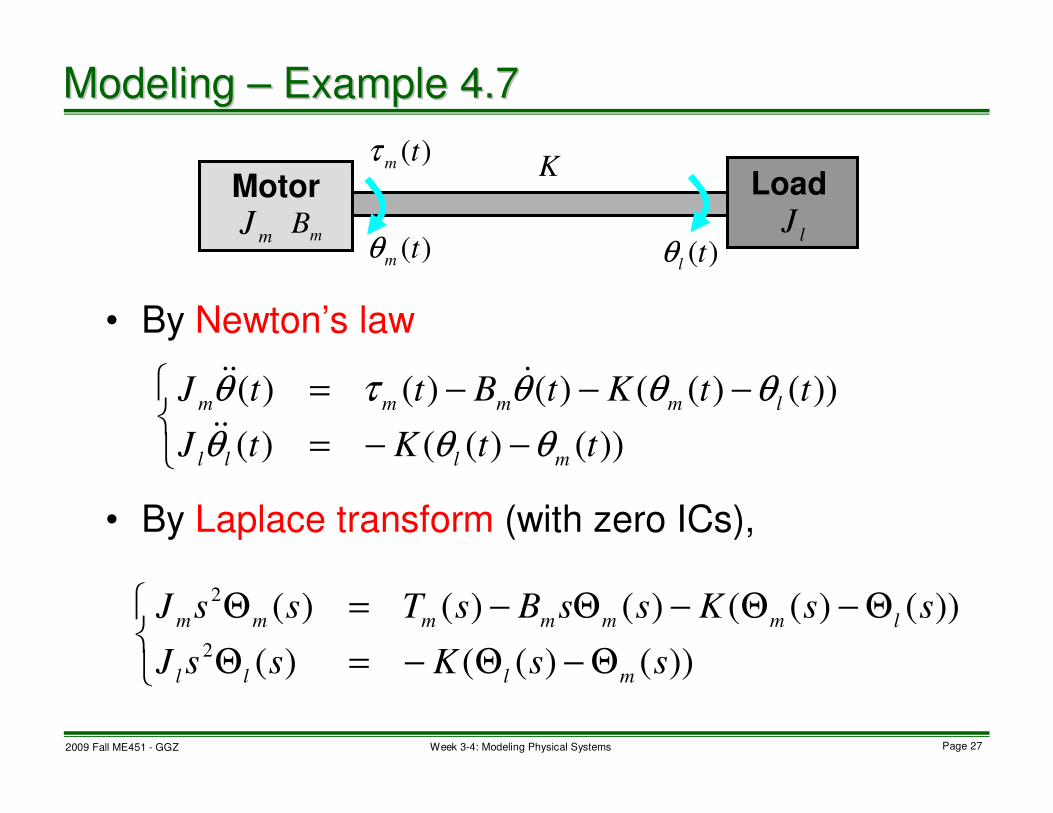
• By Newton’s law
• By Laplace transform (with zero ICs),
Modeling Modeling –– Example 4.7Example 4.7
)(tm
τ
Motor
mJ
)(tm
θm
B
K
)(tl
θ
Load
lJ
−−=
−−−=
))()(()(
))()(()()()(
ttKtJ
ttKtBttJ
mlll
lmmmm
θθθ
θθθτθ
&&
&&&
Θ−Θ−=Θ
Θ−Θ−Θ−=Θ
))()(()(
))()(()()()(2
2
ssKssJ
ssKssBsTssJ
mlll
lmmmmmm
2009 Fall ME451 - GGZ Page 28Week 3-4: Modeling Physical Systems
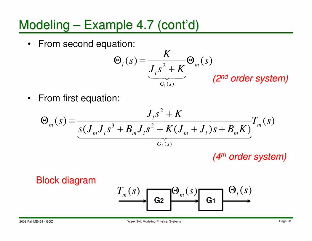
• From second equation:
• From first equation:
G2
Block diagramBlock diagram
G1
(2(2ndnd order system)order system)
(4(4thth order system)order system)
)()(
)(
2
1
sKsJ
Ks
m
sG
l
lΘ
+=Θ
43421
Modeling Modeling –– Example 4.7 (contExample 4.7 (cont’’d)d)
)(sTm
)(sm
Θ )(sl
Θ
)())((
)(
)(
23
2
2
sTKBsJJKsJBsJJs
KsJs
m
sG
mlmlmlm
l
m
4444444 34444444 21++++
+=Θ

2009 Fall ME451 - GGZ Page 29Week 3-4: Modeling Physical Systems
ThrusterThruster
Double Double
integratorintegrator
•• BroadcastingBroadcasting
•• Weather forecastWeather forecast
•• CommunicationCommunication
•• GPS, etc.GPS, etc.
)(tθ
Modeling Modeling –– Rigid Body Satellite Ex 2.13 (contRigid Body Satellite Ex 2.13 (cont’’d)d)
)(tτ)(tτ
)()( tJt θτ &&=
2
1
)(
)()(
JssT
ssG =
Θ=

2009 Fall ME451 - GGZ Page 30Week 3-4: Modeling Physical Systems
• Modeling of mechanical systems
– Translational
– Rotational
• Next, modeling of electromechanical
systems (DC-motor).
Modeling Modeling –– Summary (Mechanical System) Summary (Mechanical System)

2009 Fall ME451 - GGZ Page 31Week 3-4: Modeling Physical Systems
• Quarter car model: Obtain a transfer function from R(s) to Y(s).
Road surfaceRoad surface
M1
xx (t)(t)
KKss BB
KKww
M2y(ty(t))
AnswerAnswer
Modeling Modeling –– Additional Exercises Additional Exercises

2009 Fall ME451 - GGZ Page 32Week 3-4: Modeling Physical Systems
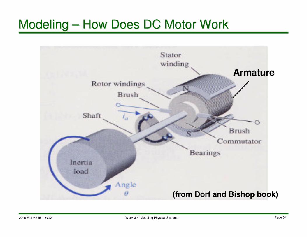
What is DC motor?
An actuator, converting electrical energy into rotational An actuator, converting electrical energy into rotational
mechanical energymechanical energy
(You will see DC motor during Labs 1 and 4.)(You will see DC motor during Labs 1 and 4.)
Modeling Modeling –– Electromechanical SystemsElectromechanical Systems

2009 Fall ME451 - GGZ Page 33Week 3-4: Modeling Physical Systems
• Advantages:
– high torque
– speed controllability
– portability, etc.
• Widely used in control applications: robot, tape drives,
printers, machine tool industries, radar tracking system,
etc.
• Used for moving loads when
– Rapid (microseconds) response is not required
– Relatively low power is required
Modeling Modeling –– Why DC motor?Why DC motor?
2009 Fall ME451 - GGZ Page 34Week 3-4: Modeling Physical Systems
ArmatureArmature
(from Dorf and Bishop book)
Modeling Modeling –– How Does DC Motor WorkHow Does DC Motor Work

2009 Fall ME451 - GGZ Page 35Week 3-4: Modeling Physical Systems
J
BBmm
Armature circuitArmature circuit Mechanical loadMechanical load
InputInput
OutputOutput
Modeling Modeling –– Model of DC MotorModel of DC Motor
)(tea )(te
m
)(tia aR aL
)(tτ
)(tlτ
)(tθ
EMFback ""
current armature:
voltageapplied:
armature":"
m
i
e
a
a
a
fricton viscous:
inertiarotor :
locityangular ve:
positionangular :
B
J
ω
θ

2009 Fall ME451 - GGZ Page 36Week 3-4: Modeling Physical Systems
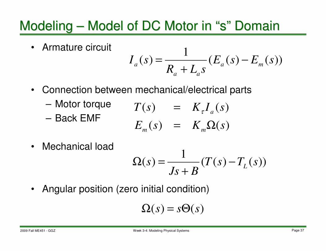
• Armature circuit
• Connection between mechanical/electrical parts
– Motor torque
– Back EMF
• Mechanical load
• Angular position
Load torqueLoad torque
)()(
)()( tedt
tdiLtiRte
m
a
aaaa++=
Modeling Modeling –– Model of DC Motor in Time DomainModel of DC Motor in Time Domain
)()(
)()(
tKte
tiKt
mm
a
ω
ττ
=
=
)()()()( ttBttJl
τθτθ −−= &&&
)()( tt θω &=
2009 Fall ME451 - GGZ Page 37Week 3-4: Modeling Physical Systems
• Armature circuit
• Connection between mechanical/electrical parts
– Motor torque
– Back EMF
• Mechanical load
• Angular position (zero initial condition)
Modeling Modeling –– Model of DC Motor in Model of DC Motor in ““ss”” DomainDomain
))()((1
)( sEsEsLR
sIma
aa
a−
+=
)()(
)()(
sKsE
sIKsT
mm
a
Ω=
=τ
)()( sss Θ=Ω
))()((1
)( sTsTBJs
sL
−+
=Ω

2009 Fall ME451 - GGZ Page 38Week 3-4: Modeling Physical Systems
Feedback systemFeedback system
Tachometer Tachometer
(Page 46)(Page 46)
Encoder Encoder
(Page 44)(Page 44)
Modeling Modeling –– DC Motor Block DiagramDC Motor Block Diagram
)(sEa
sLRaa
+
1
)(sIa
τK
)(sT
)(sTl
-
-BJs +
1 )(sΩ )(sΘ
s
1
mK
)(sEm
0)( )),()(())((
)( =Ω−++
=Ω sTsKsEBJsRsL
Ks
lma
aa
τ
0)( )),()(()(
1)( =Ω
+−−
+=Ω sEs
RsL
KKsT
BJss
a
aa
m
l
τ

2009 Fall ME451 - GGZ Page 39Week 3-4: Modeling Physical Systems
22ndnd order systemorder system
Modeling Modeling –– DC Motor Transfer FunctionDC Motor Transfer Function
)(:))((
))((1
))((
)(
)(1
sGKKBJsRsL
K
BJsRsL
KK
BJsRsL
K
sE
s
maa
aa
m
aa
a
=+++
=
+++
++=
Ω
τ
τ
τ
τ
)(:))((
)(
))((1
)(
1
)(
)(2
sGKKBJsRsL
RsL
BJsRsL
KK
BJs
sT
s
maa
aa
aa
ml
=+++
+−=
+++
+−
=Ω
ττ
)()()()()(21
sTsGsEsGsla
+=Ω
))()()()((1
)(1
)(21
sTsGsEsGs
ss
sla
+=Ω=Θ

2009 Fall ME451 - GGZ Page 40Week 3-4: Modeling Physical Systems
Note:Note: In many cases In many cases LLaa<< << RRaa. Then, an approximated TF is . Then, an approximated TF is
obtained by setting obtained by setting LLa a = 0.= 0.
11stst order systemorder system22ndnd order systemorder system
Modeling Modeling –– DC Motor Transfer Function (contDC Motor Transfer Function (cont’’d)d)
+=
+=
+=
++≈
+++=
Ω
ττ
τ
τ
τ
τ
τ
KKBR
JRT
KKBR
KK
Ts
K
KKBJsR
K
KKBJsRsL
K
sE
s
ma
a
ma
mamaaa
,: 1
:
)())(()(
)(
)1()(
)(
+=
Θ
Tss
K
sE
s
a
ττKKBJsR
R
KKBJsRsL
RsL
sL
s
ma
a
maa
aa
l++
−≈
+++
+−=
Ω
)())((
)(
)(
)(

2009 Fall ME451 - GGZ Page 41Week 3-4: Modeling Physical Systems
Negative feedback systemNegative feedback system
Memorize this!Memorize this!
Modeling Modeling –– Feedback System Transfer FunctionFeedback System Transfer Function
)(sR )(sY)(sG
)(sH
))()()()(()( sYsHsRsGsY −= )()()())()(1( sRsGsYsHsG =+
)()(1
)(
)(1
)(
)(
)(
sHsG
sG
sL
sF
sR
sY
g
g
+=
−=
−=
=
gain Loop)()()(
gain Forward)()(
sHsGsL
sGsF
g
g

2009 Fall ME451 - GGZ Page 42Week 3-4: Modeling Physical Systems
• Modeling of DC motor
– What is DC motor and how does it work?
– Derivation of a transfer function
– Block diagram with feedback
• Next
– Block Diagram
Many systems can be represented as Many systems can be represented as
transfer functionstransfer functions!!
Modeling Modeling –– Summary (DC Motor)Summary (DC Motor)

2009 Fall ME451 - GGZ Page 43Week 3-4: Modeling Physical Systems
• Suppose that u(t) is a unit impulse function and system is
at rest (zero initial conditions).
• The output g(t) for the unit impulse input is called
impulse response.
• Since U(s) = 1, the transfer function can also be defined as the Laplace transform of impulse response:
SystemSystem
Modeling Modeling –– Block Diagram (impulse response)Block Diagram (impulse response)
)()( ttu δ=
1)( =sU)(tg
)]([:)( tgLsG =

2009 Fall ME451 - GGZ Page 44Week 3-4: Modeling Physical Systems
Series connection
Modeling Modeling –– Basic TF Block Diagram (1)Basic TF Block Diagram (1)
)(1 sG )(2 sG)(sR )(sZ )(sY
)()(
)(1 sG
sR
sZ= )(
)(
)(2 sG
sZ
sY=
)()()(
)(12 sGsG
sR
sY=
)(sR )(sY)()( 21 sGsG
2009 Fall ME451 - GGZ Page 45Week 3-4: Modeling Physical Systems
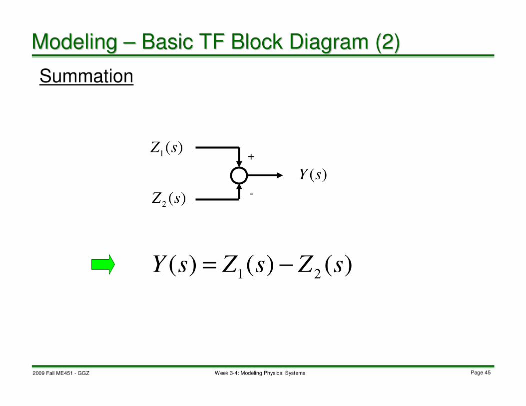
Summation
+
-
Modeling Modeling –– Basic TF Block Diagram (2)Basic TF Block Diagram (2)
)(1
sZ
)(2
sZ
)(sY
)()()(21
sZsZsY −=

2009 Fall ME451 - GGZ Page 46Week 3-4: Modeling Physical Systems
Parallel connection
)(sY
Modeling Modeling –– Basic TF Block Diagram (3)Basic TF Block Diagram (3)
)(1 sZ
)(2 sZ
)(sE)(
1sG
)(2
sG
)()(
)(1
1 sGsE
sZ=
)()(
)(2
2 sGsE
sZ=
)())()(()()()( 2121 sEsGsGsZsZsY +=+=
)()()(
)(21
sGsGsE
sY+=
)(sE )(sY)()(
21sGsG +
2009 Fall ME451 - GGZ Page 47Week 3-4: Modeling Physical Systems
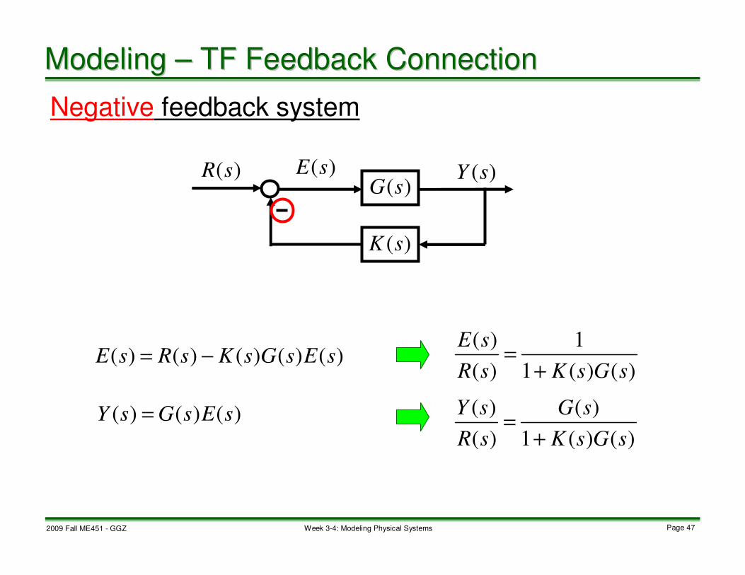
Negative feedback system
)(sE
Modeling Modeling –– TF Feedback ConnectionTF Feedback Connection
)(sR )(sY)(sG
)(sK
)()()()()( sEsGsKsRsE −=
)()()( sEsGsY =
)()(1
1
)(
)(
sGsKsR
sE
+=
)()(1
)(
)(
)(
sGsK
sG
sR
sY
+=
2009 Fall ME451 - GGZ Page 48Week 3-4: Modeling Physical Systems
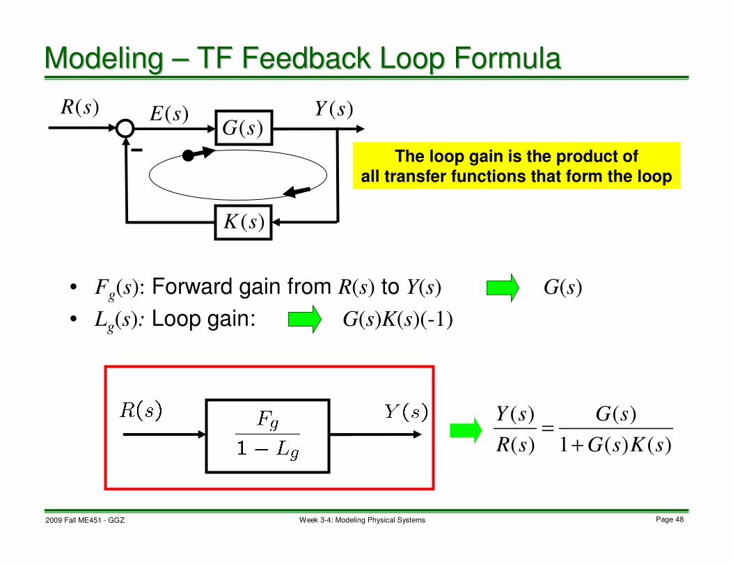
• Fg(s): Forward gain from R(s) to Y(s) G(s)
• Lg(s): Loop gain: G(s)K(s)(-1)
The loop gain is the product of
all transfer functions that form the loop
)(sG
Modeling Modeling –– TF Feedback Loop FormulaTF Feedback Loop Formula
)(sK
)(sE)(sR )(sY
)()(1
)(
)(
)(
sKsG
sG
sR
sY
+=

2009 Fall ME451 - GGZ Page 49Week 3-4: Modeling Physical Systems
Compute transfer functions from Compute transfer functions from RR((ss)) to to YY((ss).).
)(sR )(sY
)(sH
)(sR )(sY)(sG)(sG)(sC
)(sR )(sY)(sG
)(sH)(sH
)(sY)(sR
)(1
sG
)(1
sG
Modeling Modeling –– Derivation of transfer functionDerivation of transfer function

2009 Fall ME451 - GGZ Page 50Week 3-4: Modeling Physical Systems
BBmm
InputInput
OutputOutput
Modeling Modeling –– Model of DC Motor (Example 2)Model of DC Motor (Example 2)
)(tea )(te
m
)(tia aR aL
)(tτ
)(tlτ)(tθ
mgmg
R R
θ
)(tlτ)(tθ
θτ &BtB =)(
J
J
R R
θ
θsinmgmg
)(tlτ
θsinmgR
)(tτ

2009 Fall ME451 - GGZ Page 51Week 3-4: Modeling Physical Systems
• Armature circuit
• Connection between mechanical/electrical parts
– Motor torque
– Back EMF
• Mechanical load
• Angular position
)()(
)()( tedt
tdiLtiRte
m
a
aaaa++=
Modeling Modeling –– Model of DC Motor in Time DomainModel of DC Motor in Time Domain (2)(2)
)()(
)()(
tKte
tiKt
mm
a
ω
ττ
=
=
)()()()( ttBttJl
τθτθ −−= &&&
)()( tt θω &=
)()()(sin)()( smallfor
2tmgRttmgRttmR
llθτθτθ
θ
−≈−=&&

2009 Fall ME451 - GGZ Page 52Week 3-4: Modeling Physical Systems
• Armature circuit
• Connection between mechanical/electrical parts
– Motor torque
– Back EMF
• Mechanical load
• Angular position (zero initial condition)
Modeling Modeling –– Model of DC Motor in Model of DC Motor in ““ss”” DomainDomain (2)(2)
))()((1
)( sEsEsLR
sIma
aa
a−
+=
)()(
)()(
sKsE
sIKsT
mm
a
Ω=
=τ
)()( sss Θ=Ω
)),()((1
)(2
sTsTBsJs
sL
−+
=Θ )(1
)(22
sTmgRsmR
sl
+=Θ
)()(
1)(
22sT
mgRBssmRJs
+++=Θ

2009 Fall ME451 - GGZ Page 53Week 3-4: Modeling Physical Systems
Modeling Modeling –– DC Motor Block Diagram DC Motor Block Diagram (2)(2)
)(sEa
sLRaa
+
1
)(sIa
τK
)(sT
)(sTl
-
-BJs +
1 )(sΩ
)(sΘs
1
sKm
)(sEm
mgRsmR +22
)(sEa
sLRaa
+
1
)(sIa
τK
)(sT
-mgRBssmRJ +++
22 )(
1
)(sΘ
sKm
)(sEm
BsJs
mgRsmR
BsJssG
+
+
+
+=
2
22
2
1)(
1
)),()((1
)(2
sTsTBsJs
sL
−+
=Θ
)(1
)(22
sTmgRsmR
s l+
=Θ
)()(
1)(
22sT
mgRBssmRJs
+++=Θ

2009 Fall ME451 - GGZ Page 54Week 3-4: Modeling Physical Systems
Modeling Modeling –– DC Motor Transfer Function DC Motor Transfer Function (2)(2)
maa
aa
m
aa
a
KsKmgRBssmRJRsL
K
mgRBssmRJRsL
KsK
mgRBssmRJRsL
K
sE
s
τ
τ
τ
τ
+++++=
+++++
++++=
Θ
)))(((
)))(((1
)))(((
)(
)(
22
22
22
maaaKKBJsRsL
K
ssE
s
m
τ
τ
+++⋅=
Θ
=
))((
1
)(
)(
attached), pendulum (no 0 If

2009 Fall ME451 - GGZ Page 55Week 3-4: Modeling Physical Systems
BB
Modeling Modeling –– TorsionalTorsional Motion Modeling Motion Modeling (Example 2)(Example 2)
1K
)(tf
)(tθR R
m)(tx
JR R
J
Free Body DiagramFree Body Diagram
1kτ )(tθBτ
2kf
22 )( KRxfk θ−=
11 Kk θτ =
θτ &BB =
θθθ
ττθ
&
&&
BKRKRx
RfJBkk
−−−=
−−=
12
12
)(
RxKRKKBJ2
2
21)( =+++ θθθ &&&
2K

2009 Fall ME451 - GGZ Page 56Week 3-4: Modeling Physical Systems
Modeling Modeling –– TorsionalTorsional Motion Modeling Motion Modeling (Example 2)(Example 2)
)(tf
m)(tx
Free Body DiagramFree Body Diagram
2kf22 )()()()( KRxtftftfxm k θ−−=−=&&
)()(
)(2
21
2
2 sXRKKBsJs
RKs
+++=Θ
θRKtfxKxm 22 )( +=+&&
))()((1
)(2
2
2sRKsF
KmssX Θ+
+=

2009 Fall ME451 - GGZ Page 57Week 3-4: Modeling Physical Systems
)(sF
2
2
1
Kms +
)(sΘ
RK2
+
222
221
22
2
2
221
22
2
222
221
22
2
2
))()((
))()((
))()((
1)(
RKRKKBsJsKms
RK
RKKBsJsKms
RK
RKKBsJsKms
RK
sG−++++
++++
++++=
−=
Modeling Modeling –– TorsionalTorsional Motion Modeling Motion Modeling (Example 2)(Example 2)
)( 2
21
2
2
RKKBsJs
RK
+++
)()(
)(2
21
2
2 sXRKKBsJs
RKs
+++=Θ))()((
1)(
2
2
2sRKsF
KmssX Θ+
+=
212
22
212
34
2
)]([ )(
KKBsKsRKKmJKmBsmJs
RKsG
++++++=

2009 Fall ME451 - GGZ Page 58Week 3-4: Modeling Physical Systems
• Block diagrams
– Elementary diagrams
– Feedback connections
• Next
– Linearization
Modeling Modeling –– Summary (Block Diagram)Summary (Block Diagram)

2009 Fall ME451 - GGZ Page 59Week 3-4: Modeling Physical Systems
• A system having Principle of Superposition
A nonlinear system does not satisfy the
principle of superposition.
SystemSystem
Modeling Modeling –– What Is a Linear System?What Is a Linear System?
)(tu )(ty
ℜ∈∀
+→+⇒
→
→
21
22112211
22
11
,
)()()()()()(
)()(
αα
αααα tytytututytu
tytu
linearnot is )0( )(function affineAn ≠+= bbaxtf

2009 Fall ME451 - GGZ Page 60Week 3-4: Modeling Physical Systems
• Easier to understand and obtain solutions
• Linear ordinary differential equations (ODEs),
– Homogeneous solution and particular solution
– Transient solution and steady state solution
– Solution caused by initial values, and forced solution
• Add many simple solutions to get more complex ones (use
superposition!)
• Easy to check the Stability of stationary states (Laplace Transform)
Modeling Modeling –– Why Linear System?Why Linear System?

2009 Fall ME451 - GGZ Page 61Week 3-4: Modeling Physical Systems
• Actual physical systems are inherently nonlinear. (Linear
systems do not exist!) Ex. f(t)=Kx(t), u(t)=Ri(t)
• TF models are only for Linear Time-Invariant (LTI) systems.
• Many control analysis/design techniques are available only
for linear systems.
• Nonlinear systems are difficult to deal with mathematically.
• Often we linearize nonlinear systems before analysis and design. How?
Modeling Modeling –– Why LinearizationWhy Linearization

2009 Fall ME451 - GGZ Page 62Week 3-4: Modeling Physical Systems
• Nonlinearity can be approximated by a linear function for
small deviations δx around an operating point x0
• Use a Taylor series expansion at x0
Linear approximation
Nonlinear function
Operating point x0
Old coordinate
New coordinate
Modeling Modeling –– How to How to LinearizeLinearize It?It?
)(0
xxf δ+
)(xf
x
xδ
2009 Fall ME451 - GGZ Page 63Week 3-4: Modeling Physical Systems
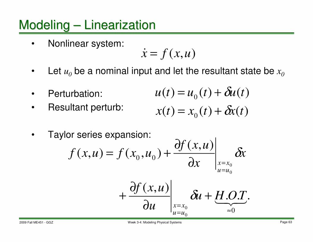
• Nonlinear system:
• Let u0 be a nominal input and let the resultant state be x0
• Perturbation:
• Resultant perturb:
• Taylor series expansion:
Modeling Modeling –– LinearizationLinearization
),( uxfx =&
)()()( 0 tututu δ+=
)()()( 0 txtxtx δ+=
...),(
),(),(),(
0
00
0
0
0
0
321≈=
=
=
=
+∂
∂+
∂
∂+=
TOHuu
uxf
xx
uxfuxfuxf
uuxx
uuxx
δ
δ

2009 Fall ME451 - GGZ Page 64Week 3-4: Modeling Physical Systems
Note that ; hence
L. sys.L. sys.N. sysN. sys
Modeling Modeling –– Linearization (contLinearization (cont’’d)d)
uu
uxfx
x
uxfuxfxx
uuxx
uuxx
δδδ
0
0
0
0
),(),(),(
000
=
=
=
= ∂
∂+
∂
∂+=+ &&
),(000
uxfx =&
uu
uxfx
x
uxfx
uuxx
uuxx
δδδ
0
0
0
0
),(),(
=
=
=
= ∂
∂+
∂
∂=&
u x uδ
0u
),(000
uxfx =&
xδ
0x
xxx δ+=0uuu δ+=
0

2009 Fall ME451 - GGZ Page 65Week 3-4: Modeling Physical Systems
• Motion of the pendulum
• Linearize it at
• Find u0
• New coordinates:
Modeling Modeling –– Pendulum LinearizationPendulum Linearization
)()(sin)(2tutmgLtmL =+ θθ&&)(tu
)(tθ
mg
L
0)()(sin
)(
),(
2=−+
44 344 21
&&
uf
mL
tu
L
tgt
θ
θθ
πθ =0
00sin
02
0=→=−+ u
mL
u
L
g ππ&&
uuuu δδ
δθπδθθθ
+=+=
+=+=
00
0

2009 Fall ME451 - GGZ Page 66Week 3-4: Modeling Physical Systems
• Taylor series expansion of at
Modeling Modeling –– Pendulum Linearization (contPendulum Linearization (cont’’d)d)
),( uf θ .0 , == uπθ
L
g
L
guf
u
−==∂
∂
==
=πθ
πθ
θ
θ
θ cos),(
0
2
0
1),(
mLu
uf
u
−=∂
∂
=
=πθ
θ
0),(),(
00
=∂
∂+
∂
∂+
=
=
=
=
uu
ufuf
uu
δθ
δθθ
θθδ
πθπθ
&&
01
2=−− u
mLL
gδδθθδ &&

2009 Fall ME451 - GGZ Page 67Week 3-4: Modeling Physical Systems
• TF derivation
• The more time delay is, the more difficult to control
(Imagine that you are controlling the temperature of your shower with a very long hose. You will either get burned
or frozen!)
(Memorize this!)
Modeling Modeling –– Time Delay Transfer FunctionTime Delay Transfer Function
delay time is where),()(dd
TTtxty −=
L
sTsT dd esX
sYsXesY
−−=⇒=
)(
)( )()(
1
11)0(
)(
0
0 +=⇒+=−
∂
∂+≈
−
=
= sTesTs
s
eee
d
sT
d
s
sT
s
sTsT d
d
dd

2009 Fall ME451 - GGZ Page 68Week 3-4: Modeling Physical Systems
• Step One: identify the system model’s input r(t) and output y(t).
• Step Two: express model in form
• Step Three: define equilibrium operation point r0 and y0 ,
and setting all their corresponding derivatives to zero at
equilibrium point
• Perform Taylor expansion about (r0,c0) retaining only 1st
order derivatives
• Step Five: change variables to deviations:
• Step Six: rewrite the function defined in Step 5 in standard
ODE.
Modeling Modeling –– Summary: Steps of LinearizationSummary: Steps of Linearization
0,...),,...,,( =yyrrf &&
,...).0,0,...,0,0(0000
==== yyrr &&&&&&
,...).~,~,...,~,~(000000
yyyyyyrrrrrr &&&&&& −=−=−=−=

2009 Fall ME451 - GGZ Page 69Week 3-4: Modeling Physical Systems
Modeling Modeling –– 6 Step Example 16 Step Example 1
)( :output system ),( :input System ttu θ
)()(sin)(2tutmgLtmL =+ θθ&&
0)()(sin
)(
),,(
2=−+
4444 34444 21
&&
&& uf
mL
tu
L
tgt
θθ
θθ
System ODE:System ODE:
Step One (input/output):Step One (input/output):
Step Two Step Two ((f f ((……)=0):)=0):
Step Three Step Three ((θθ00, u, u00))::
,0 and ,Let 000
=== θθπθ &&&
00sin
02
0=→=−+ u
mL
u
L
g πθ&&

2009 Fall ME451 - GGZ Page 70Week 3-4: Modeling Physical Systems
Modeling Modeling –– 6 Step Example 1 6 Step Example 1 (cont(cont’’d)d)
)0(1
)0()(
)0(1
)0(1)(cos
)()()( ),,(),,(
2
2
000
0
000
0
0
0
0
0
0
0
0
0
−−−+−=
−−−⋅+−=
−∂
∂+−
∂
∂+−
∂
∂+≅
=
=
=
=
=
=
=
=
=
=
umLL
g
umLL
g
uuu
fffufuf
uuuuuu
θπθ
θπθθ
θθθ
θθθ
θθθθ
πθ
θθ
θθ
θθ
θθ
θθ
θθ
&&
&&
&&&&&&43421
&&&&
&&&&&&&&&&&&
Step Four (Taylor expansion):Step Four (Taylor expansion):
Step Five Step Five ((δδθθ00, , δδuu00))::
01
),,(2
=−+≅ umLL
guf δδθθδθθ &&&&
Step Six Step Six (rewrite(rewrite))::
mLgsmLsU
su
mLL
g
+=
∆
∆Θ⇒=+
222
1
)(
)(1δδθθδ &&

2009 Fall ME451 - GGZ Page 71Week 3-4: Modeling Physical Systems
Modeling Modeling –– 6 Step Example 26 Step Example 2
System ODE:System ODE:
2)( :force drag cAerodynami
)( :forcefriction Viscous
)( :input force Tractive
vKtff
vKtff
tff
add
vvv
mm
==
==
=
2vKvKffffvm
avmvdm−−=−−=&
mf
df
vf
mavfvKvKvm =++
2&
kgm
mNK
mNK
mv
a
v
1000
/sec0.1
sec/ 1.0
sec/ 30
22
0
=
−=
−=
=

2009 Fall ME451 - GGZ Page 72Week 3-4: Modeling Physical Systems
Modeling Modeling –– 6 Step Example 2 6 Step Example 2 (cont(cont’’d)d)
)( :(velocity)output system ),( :force) (tractiveinput System tvtfm
Vehicle System:Vehicle System:
Step One (input/output):Step One (input/output):
Step Two Step Two ((f f ((……)=0):)=0):
Step Three Step Three ((vv00,vdot,vdot00 uu00))::
000 find and 0, and 30Let m
fvv == &
NvKvKfavm
903301301.0 22
000 =×+×=+=
mavfvKvKvm =++
2&
0
),,(
2=−++
444 3444 21&
&vvff
mav
m
fvKvKvm

2009 Fall ME451 - GGZ Page 73Week 3-4: Modeling Physical Systems
Modeling Modeling –– 6 Step Example 2 6 Step Example 2 (cont(cont’’dd--1)1)
0)()()2()(10
)()()( ),,(),,(
0000
000
0
000
0
0
0
0
0
0
0
0
0
=−+−⋅++−−=
−∂
∂+−
∂
∂+−
∂
∂+≅
=
=
=
=
=
=
=
=
=
vvmvvvKKff
vvv
fvv
v
fff
f
fvvffvvff
avmm
vvvv
ff
vvvv
ffmm
vvvv
ffm
mmmmmmmm
&&
&&&4434421
&&
&&&&&&
Step Four (Taylor expansion):Step Four (Taylor expansion):
Step Five Step Five :)~
,~,~
(000
vvvvvvfffmmm
&&& −=−=−=
Step Six Step Six (rewrite(rewrite))::
0~~)2(
~
1.6030121.0
0
1000
=−⋅++
=××+
mavfvvKKvm
43421&
1.601000
1
)(
)(~~1.60~
1000+
=⇒=+ssF
sVfvv
m
m&

2009 Fall ME451 - GGZ Page 74Week 3-4: Modeling Physical Systems
Modeling Modeling –– 6 Step Example 36 Step Example 3
1R
C
ivovRv
)(ti
)()()(1
)(0
0
0tvCtidi
Ctv
t
&=⇒= ∫ ττ
)()()( 3
22212tiRtiRtV
R+=
)()()()()( 0
3
22211 tvtiRtiRRtvi
+++=
)()()()()(0
3
0
3
220211tvtvCRtvCRRtv
i+++= &&
2
22211 /200 and ,1 ,1 ARRR Ω=Ω=Ω=
,1.0 FC = )()(2.0)(2.0)( 0
3
00 tvtvtvtvi
++= &&
VvVvi 5 and 10at it Linearize 0 ==

2009 Fall ME451 - GGZ Page 75Week 3-4: Modeling Physical Systems
Modeling Modeling –– 6 Step Example 3 6 Step Example 3 (cont(cont’’d)d)
)( :tageoutput vol system ),( :ageinput volt System0
tvtvi
Circuit System:Circuit System:
Step One (input/output):Step One (input/output):
Step Two Step Two ((f f ((……)=0):)=0):
Step Three Step Three ((vv00,vdot,vdot00 vvii))::
00 find and 5, and 10Let vvvi
&==
solution) real(only 81.2025 00
3
0 =⇒=−+ vvv &&&
)()(2.0)(2.0)(0
3
00tvtvtvtv
i++= &&
0)()()(2.0)(2.0
),,(
0
3
00
00
=−++44444 344444 21
&&
&vvvf
i
i
tvtvtvtv

2009 Fall ME451 - GGZ Page 76Week 3-4: Modeling Physical Systems
Modeling Modeling –– 6 Step Example 3 6 Step Example 3 (cont(cont’’dd--1)1)
0)81.2(938.4)5(1)10(10
)81.2()5()10( )81.2,5,10(),,(
0
6.02.0
0
0
81.2510
0
0
81.2510
0
81.2510
0
00
20
0
0
0
0
0
0
=−+−⋅+−⋅−=
−∂
∂+−
∂
∂+−
∂
∂+≅
×+
=
=
=
=
=
=
=
=
=
vvv
vv
fv
v
fv
v
ffvvvf
v
i
vvv
vvv
i
vvv
i
iiii
&321
&&4434421
&
&
&&&
Step Four (Taylor expansion):Step Four (Taylor expansion):
Step Five Step Five :)81.2~
,5~,10~(000
−=−=−= vvvvvvii
&&
Step Six Step Six (rewrite(rewrite))::
0~~~938.4
00=−+
ivvv&
1938.4
1
)(
)(~~~938.4 0
00+
=⇒=+ssV
sVvvv
i
i&

2009 Fall ME451 - GGZ Page 77Week 3-4: Modeling Physical Systems
Modeling Modeling –– 6 Step Example 3 6 Step Example 3 (cont(cont’’dd--2)2)
0)0(2.0)10(1)10(10
)0()10()10( )0,10,10(),,(
00
0
01010
0
0
01010
0
01010
0
00
0
0
0
0
0
0
=−⋅+−⋅+−⋅−=
−∂
∂+−
∂
∂+−
∂
∂+≅
=
=
=
=
=
=
=
=
=
vvv
vv
fv
v
fv
v
ffvvvf
i
vvv
vvv
i
vvv
i
iiii
&
&&43421
&
&&&
Step Four (Taylor expansion):Step Four (Taylor expansion):
Step Five Step Five :)0~
,10~,10~(000
−=−=−= vvvvvvii
&&
Step Six Step Six (rewrite(rewrite))::
0~~~2.0
00=−+
ivvv&
12.0
1
)(
)(~~~2.0 0
00+
=⇒=+ssV
sVvvv
i
i&
Step Three Step Three ((vvoo==1010 vvii==1010))::
solution) real(only 00 00
3
0 =⇒=+ vvv &&&

2009 Fall ME451 - GGZ Page 78Week 3-4: Modeling Physical Systems
• Modeling of
– Nonlinear systems
– Systems with time delay
• Next
– Time response of physical systems
Modeling Modeling –– Linearization SummaryLinearization Summary