MODELING OPEN SPACE ACQUISITION IN BOULDER, COLORADO

by

Kathryn Metivier

A Thesis Presented to the

FACULTY OF THE USC GRADUATE SCHOOL

UNIVERSITY OF SOUTHERN CALIFORNIA

In Partial Fulfillment of the

Requirements for the Degree

MASTER OF SCIENCE

(GEOGRAPHIC INFORMATION SCIENCE AND TECHNOLOGY)

May 2015

Copyright 2015 Kathryn Metivier

ii

DEDICATION

I dedicate this thesis to my five children for sharing my time and attention with years of academia.

My wish for each of them is to succeed in their personal endeavors and never consider themselves

too old or too young to accomplish their goals. Thank you to my family for their constant support

and encouragement, their intellectually and environmentally conscious conversations, and for

reminding me what is most important in life.

iii

ACKNOWLEDGMENTS

I would like to thank the City of Boulder, Colorado Open Space and Mountain Parks staff for

making the MOSA model possible by sharing their resource management expertise. While

employed as a GIS Technician for OSMP I built the MOSA model for the real estate

acquisition team to use as a supplemental guide in open space parcel selection. The City of

Boulder holds no liability for the content of this thesis. I would also like to thank the

University of Colorado in Boulder Geography Department at for my extensive undergraduate

preparation in technical geography. Special thanks are reserved for the GIST graduate faculty

of the Spatial Science Institute at the University of Southern California for their unequivocal

encouragement and impeccable instruction. I am blessed with the opportunity to study,

practice, apply, and problem solve geospatial science.

iv

TABLE OF CONTENTS

CHAPTER ONE: INTRODUCTION 1

1.1 Motivation of Research: Why Open Space Matters 2

1.2 Background: Qualifying Open Space 3

1.3 Study Area: Boulder, CO 5

CHAPTER TWO: RELATED WORK IN MODELING OPEN SPACE PRIORITIZATION 8

2.1 Examples of Land-use Prioritization Models 11

CHAPTER THREE: METHODS OF MODELING OPEN SPACE ACQUISITION (MOSA) 15

3.1 Source Criteria in MOSA 15

3.2 Data Collection and Sources 17

3.3 Modeling Open Space Acquisition Methodology 19

3.3.1 Parcel Selection Model 22

3.3.2 Wildlife Model 25

3.3.3 Riparian Model 28

3.3.4 Oil and Gas Model 29

3.3.5 Cultural Model 30

3.3.6 Recreation Model 30

3.3.7 Agriculture Model 31

3.3.8 Vegetation Model 32

3.3.9 Proximity Model 32

3.3.10 Classification Methods 36

3.3.11 Final Weighted Criteria Model 38

Dedication ii

Acknowledgments iii

List of Tables vi

List of Figures vii

List of Abbreviations viii

Abstract ix

v

CHAPTER FOUR: MOSA RESULTS 42

4.1 MOSA Results in Detail 42

CHAPTER FIVE: FUTURE WORK AND CLOSING DISCUSSION 48

5.1 Future Model Considerations and Limitations 48

5.2 Closing Discussion 51

REFERENCES 54

APPENDIX A: Weighted Criteria Analysis using Jenks Classification Method on Pixels 58

APPENDIX B: Original MOSA Parcels with Above Average Suitability Index 59

APPENDIX C: Adjusted MOSA Parcels with Above Average Suitability Index 60

vi

LIST OF TABLES

Table 3.1: MOSA Public Data Sources Available Online 17

Table 3.2: MOSA Data Sources and Metadata 18

Table 3.3: City Council Priority Criterion 22

Table 3.4: Wildlife Subclass Criteria Ranking in MOSA on a Scale of 1-9 25

Table 3.5: Riparian Data Structure in Mosa 28

Table 3.6: Example of Reclassification of Near Distance and Size in MOSA 35

Table 3.7: Original MOSA Suitability Indices using Jenks Classification 38

vii

LIST OF FIGURES

Figure 1.1: Sample Area Of Boulder Colorado 7

Figure 2.1: An Example of Using Gis Data Layers In Criteria Modeling 8

Figure 2.2: Effective Methodologies Of Land-Use Modeling 11

Figure 3.1: Private Parcel Selection Model 23

Figure 3.2: The Available Land within the Priority Areas Of Boulder, Co 24

Figure 3.3: Wildlife Model in Mosa 27

Figure 3.4: Riparian Model in Mosa 29

Figure 3.5: Oil and Gas Model in Mosa 29

Figure 3.6: Cultural Model in Mosa 30

Figure 3.7: Recreation Model in Mosa 31

Figure 3.8: Agriculture Model in Mosa 31

Figure 3.9: Vegetation Model in Mosa 32

Figure 3.10: Proximity Model in Mosa 33

Figure 3.11: Quantile Classification Method upon Pixels 36

Figure 3.12: Jenks Natural Breaks Classification Method upon Pixels 37

Figure 3.13: The Final Weighted Class Criterion in MOSA 39

Figure 3.14: Zonal Statistics and Distribution of Mosa Data by Sample Area 40

Figure 3.15: Example Open Space Parcel Rating Sheet 41

Figure 4.1: Mosa Targeted Parcels from the Top Four Jenks Classifications 43

Figure 4.2: Spatial Distribution Comparison of Parcel Suitability Indices 46

Figure 4.3: Parcel Criterion Comparison 47

viii

LIST OF ABBREVIATIONS

AAG Association of American Geographers

BOCO Boulder County

BVCP Boulder Valley Comprehensive Plan

CE Conservation Easement

CNHP Colorado Natural Heritage Program

COGCC Colorado Oil and Gas Conservation Commission

COB City of Boulder

COMAP Colorado Ownership Management and Protection

CPW Colorado Parks and Wildlife

FEMA Federal Emergency Management Agency

GIS Geographic Information Science

GIST Geographic Information Science and Technology

HCA Habitat Conservation Area

MOSA Modeling Open Space Acquisition

NDIS Natural Diversity Information Source

NDVI Normalize Difference Vegetation Index

NHD National Hydrographic Dataset

OSMP Open Space and Mountain Park

USDA United States Department of Agriculture

USGS United States Geological Survey

ix

ABSTRACT

Purchasing land for open space use is crucial for municipalities that are concerned with

conserving land and mitigating urban sprawl. Land-use modeling measures the ecological value

of a parcel, with budget constraints in mind, as an ecological vs. economic tradeoff. This thesis

develops a land-use modeling system termed Modeling Open Space Acquisition (MOSA) that

quantifies the ecological value of land targeted for open space acquisition. MOSA is designed as

a decision support tool for local policymakers to identify ecologically rich parcels that can be

targeted by using a multi-criteria model. Each parcel in the study area (Boulder, Colorado) is

ranked by weighted criteria generated from a variety of data sources. The weighted criteria

include wildlife habitat, agricultural lands, historical sites, recreation corridors, vegetation

biodiversity, riparian wetlands, parcel proximity, and parcel size. While other weighted land-use

models primarily use vector data (i.e., shapes with defined boundaries), the MOSA approach

developed here uses raster data. Each cell in the raster dataset represents 150 square feet in the

study area. In a parcel, the numerical average of the parcel’s cell values represents its ecological

contribution, which can be used to determine highly natural resourced land and to provide

supplemental evidence to quantifying, targeting, and prioritizing parcel acquisition for

preservation. Governing agencies can benefit from land-use modeling like MOSA where parcel

acquisition is evaluated from a scientific classification of natural resource capital over a parcel’s

economic value alone.

1

CHAPTER ONE: INTRODUCTION

Open space can be defined as land that is unobstructed by development and accessible to the

public. Ecological contributions from natural resources add to the benefits of open space parcel

purchase. Land resource quality can be quantified by overlaying ecological spatial data into a

multiple criteria Geographic Information System (GIS) environment, where each data input is

assigned a level of priority decided upon by city planners. Ideally, the parcels with greater than

average ecological value can help city planners to justify their acquisition for open space.

Protecting land for open space is increasingly critical for environmental health; it

connects communities and mitigates urban sprawl. The numerous ways of prioritizing, planning,

and protecting land’s intrinsic beauty vary between political, economic, and ecological contexts.

Whether a parcel contains rare flora or fauna, produces agriculture, or serves as a contiguous

byway for urban connectivity, the land can be valued both monetarily and ecologically. This

dichotomy raises traditional debates between open space preservation and the monetary

expenditure required to acquire it. Ecologists may argue that economists are “narrow and

anthropocentric” when viewing the importance of ecological systems because they tend to focus

on the immediate impacts rather than the long term and indirect implications to ecosystem

integrity (Bockstael et al. 1995).

Economists are often impatient with ecologists for disregarding human preferences in

land-use and urban development. Decision makers analyze the benefits of recreational

opportunity, open space contiguity, and habitat conservation, often under the political pressures

of taxpaying citizens and interest groups. Other concerns of open space acquisition include

budget constraints, justification of purchase, management, and public scrutiny. Unfortunately,

many decision makers rank economic value of land more heavily than ecological value, which

2

can lead to purchasing parcels with few contributions toward environmental wellbeing. Land-use

modeling enables public agencies to objectively rank a criterion that classifies land by its natural

capital. This thesis develops a GIS based parcel prioritization system termed Modeling Open

Space Acquisition (MOSA) to classify land by its ecological value prior to parcel purchase.

1.1 Motivation of Research: Why Open Space Matters

Open space provides ecological services for human health. The vast benefits that parks

and natural areas provide are complemented by wetlands, forests, and wildlife habitat, where

open space provide aesthetic benefits in growing metropolitan areas and may offer relief from

congestion and other negative effects of land development (McConnell and Walls 2005). When a

community embraces the value of open space and connects with its environment, it can lead to

the paradigm shift described by Aldo Leopold when he writes, “We abuse land because we see it

as a commodity belonging to us. When we see land as a community to which we belong, we may

begin to use it with love and respect” (Leopold 1949, 8). When open space is selected carefully

and managed appropriately its eco-services contribute greatly to a community’s quality of life.

The community that embraces the cost benefits of public land is likely more willing to support

land acquisition taxation. The financial contributions of future generations are deemed the

measurement of a community’s willingness to protect and preserve intrinsic natural land

(Bradley 2010).

The United States Department of Interior has long practiced funding the purchase of

public lands through tax dollars for habitat conservation. The US National Wildlife Refuge

System Improvement Act of 1997 directs the Secretary of the Interior to strategically plan and

strive for continued growth toward the benefit of ecosystem conservation (Gergely et al. 2000).

3

As a result of congressional mandates, conservation lands are devoted to preserving the natural

habitat of native vertebrates, macroscopic invertebrates, vegetative communities, agriculture

production, and other categories of ecosystems and ecological integrity. Local and federal

government rely heavily on taxpaying citizens to support and fund open space acquisition.

Recreational use at these public parks through entrance, membership, and commerce fees

subsidize the cost of public land management and may increase intrinsic public perception by

connecting with nature through personal experience. Citizens who enjoy their surroundings in

open space and park recreation are more willing to support land acquisition (Erickson 2006).

1.2 Background: Qualifying Open Space

Land can be qualified by its level of ecological value prior to considering it for open

space. Ecological systems provide crucial life supporting interdependence that is beneficial to

gross national product and to human health. Recent conservation prioritization efforts claim the

ability to synergistically conserve bio-diverse ecosystem services that preserves ecologic

functions in nature while contributing to the wellbeing of humanity (Izquierdo 2012).

Functioning ecosystems can be classified by their quality of biological habitat and their

contribution toward human welfare, both directly and indirectly. For example, this can include

preservation of wildlife corridors, protecting wetlands, watersheds, and air quality. It might also

include development of advantageous natural environments like recreational hiking and biking

trails or city parks and connective greenbelts throughout an urban area. Humans often neglect the

value of these ecological services and disagree about preserving them. Ecosystem services are

often neglected in commercial market evaluation and policy decision-making when compared

with traditional economic and manufactured capital that may compromise the sustainability of

mankind (Costanza et al. 1997). Economic, ecologic, and sociologic conditions vary over time in

4

an ecosystem where humans coexist with nature; thus people’s attitudes towards open space

preservation and their willingness to support it will also vary (Gomez-Pompa et al. 1992).

Prioritizing areas for preservation should be based on clear objectives that state the intent

of the open space plan and program. Most communities agree on the benefits of sustainable

ecological services as general goals of open space preservation. These benefits include

preserving town character and limiting urban sprawl. Protecting natural resources and wildlife

habitats to ensure public health and safety are also contributions of open space. Recreational

benefits of managed trail systems enhance the visitor’s experience through hiking and biking

while preserving greenways provide connective byways from the city to the suburbs. Agriculture

is another added benefit of maintaining open space for farmers growing locally and organically.

Qualifying open space is one challenging issue in land-use planning. Acquiring real

estate for open space is described as a combination of natural resources where the greatest value

is in the sum of their individual parts (Miles et al. 1996). Highly creative planning in parcel

selection is an effective combination of financial resources and professional skills working

synergistically to create land that is economically sound, aesthetically pleasing, and

environmentally responsive. There are many considerations of parcel selection: its size, its

proximity to other protected land, its recreational benefits, the presence of wetland or critical

habitat, and importantly, its price if the owner is willing to sell. Standard real estate appraisal is

often based on the market value of nearby properties. Land-use priority can also determine the

value of a parcel at a given price when the appraisal may not arrive at market value when one

considers the parcel’s planned use of development (Friedman 1990). The parcel in close

proximity to existing open space land that connects a recreational corridor may be worth the

extra expenditure, as opposed to a parcel with fewer assets. Some residents are hesitant to sell at

5

any given value and would require sufficient incentives to sell their land (McDonald et al. 2001).

With many issues at hand city planners weigh the cost benefits of open space valuation and often

must explain why they choose to purchase one parcel over another (Czech 2001).

1.3 Study Area: Boulder, CO

Boulder, CO offers the unique case study of wilderness that has high intrinsic value to its

citizens and is largely managed as public land. Private land is also highly valued, and city

planners regulate land use to conserve and protect habitat biodiversity. This thesis develops a

local case study of an ideal land conservation model for Boulder, Colorado, located

approximately at 40.00 latitude and -105.17 longitude.

Boulder is distinguished by the city being mostly surrounded by public open space,

conservation easements, county public land, subdivisions, or privatized agricultural lands worth

great value. However, because the city annexation limit has had a no-growth policy since 1967,

the land within the study area exhibits the influence of an urban island price bubble, which

inherently inflates the cost of open space acquisition (Power and Turvey 2010). Between the

years of 1950 and 1970 Boulder experienced massive population and commercial growth at the

rate of around 6.0% per year. The citizens quickly passed many growth control ballots in the

following years limiting the number of jobs supported within the city limits and how many new

dwellings are built. Aggressive open space land purchases and urban control policy have limited

population growth in Boulder to nearly 0.5% per year for the past decade. Because of

progressive foresight in urban planning, Boulder is one of the first cities in North America to

publicly purchase and manage a prime open space landscape.

6

A growing urban economy allows a significant tax base with which to purchase public land

to mitigate urban sprawl. However, such land is often expensive in high demand areas. Citizens

within the Boulder community generally pride themselves in supporting ecosystem conservation

while sustaining a balanced coexistence with nature. Through self-imposed sales taxation,

citizens have voted to support land acquisition, which adds annually to the approved city council

budget for land acquisition, restoration, and management. In 1967 Boulder, CO citizens made

history by voting 77% in favor of a sales tax specifically to buy and maintain natural lands. This

election marked the first time voters in any United States city passed a self-imposed sales tax in

support of open space land acquisition for preservation. Previously, in 1959 Boulder’s charter

was amended to include the “Blue Line,” which set the western edge of the city at an elevation,

where sewer and water services are unavailable, as an attempt to mitigate development while

preserving Boulder’s mountain backdrop.

The City of Boulder owns and manages more than 46,000 acres of Open Space and

Mountain Parks land in and around Boulder, Colorado. The very first piece of land, 80 acres at

the base of Flagstaff Mountain, was purchased by the city in 1898 to be used as one in a series of

Chautauqua cultural centers around the country. Since then, the Open Space program has

acquired over 400 separate properties. The study area in and around Boulder, CO includes

89,238 acres (Figure 1.1). The study area includes four subsections: Table Mountain, Mountain

Parks, Jefferson County Partnership, and the Boulder Valley Comprehensive Plan Accelerated

Area (City of Boulder Land Acquisition Report 2013).

7

Figure 1.1: Sample Area of Boulder, CO

The remainder of this thesis is organized as follows: Chapter 2 describes work related to

the problem of modeling open space prioritization; Chapter 3 introduces the land-use model

(MOSA) created in this thesis then details its methodology; Chapter 4 discusses the MOSA

model results and interrogates the sensitivity of the MOSA land-use criterion; and Chapter 5

concludes with future model considerations and closing discussion.

8

CHAPTER TWO: RELATED WORK IN MODELING OPEN SPACE

PRIORITIZATION

Municipalities like the City of Boulder can benefit from land-use modeling because parcels

considered for acquisition can be examined spatially prior to its acquisition. The research of

land-use modeling includes multi-criteria decision making land-use modeling using expert based

priority ranking with the intent of classifying a parcel’s natural values. The model outcome

identifies hot spots where land is most ecologically significant, thus providing evidence to

prioritize parcels for open space purchase.

Digital GIS data layers in land-use modeling are defined spatially and are collected by

reliable sources. Effective land-use models consider digital data representation of specific types

of real world phenomena. Ecological models are specific to a particular geographic region and

simulate the complex dynamics of a natural ecosystem (Watzhold et al. 2005). Figure 2.1 from

the City of Rocky Mount, NC shows sample data inputs in GIS map overlay that can translate

different parameters depending on the decision maker’s choices.

Figure 2.1: An Example of using GIS Data Layers in Criteria Modeling

Graphic Provided by the City of Rocky Mount, NC

9

Multiple criteria evaluation is the process of ranking a set criteria outlined by an

expert(s). Human interaction such as between city planners, city council, and taxpayers’ support

serves as the “expert” that determines the relative importance of set criteria. Several benefits to

multi-criteria decision making are: 1) it accounts for multiple and conflicting criteria, 2) it

supports the management of ecosystem services, 3) it models a criteria structure open for

discussion, and 4) it offers a process that leads to rational, justifiable, and explainable decisions

(Mendoza and Martins 2006).

Additional benefits of multi-criteria modeling is that human experts can interact with

planning objectives, both qualitative and quantitative measurements, within an environmental

context. The spatial relationships between interacting variables will therefore present

recognizable patterns or tendencies of likeliness, thus aiding the recognition of ecological

clusters (Lei et al. 2005). Expert opinion based land-use models employ various mixed data sets

to represent real-world criterion to determine these spatial patterns in relation to set criterion. The

adaptive decisions of a growing city or changing budget constraints are two criteria outside of

ecological values that experts could bring to multi-criteria model.

Some challenges with modeling environmental simulation are the purpose that model

serves, the operational dynamics within the model, and the extent of model replication,

validation, and functionality to ultimately be communicated and shared with others (Crooks,

Castle, and Batty 2008). When classifying any ecological criteria for open space acquisition a

model should be adaptive with interchangeable data layers, functional with consistent results,

replicable for others to adopt, and modifiable to support the interactions of expert opinion that

change over time. The MOSA approach built in this thesis is a flexible and functional land-use

model because the criteria ranking and inputs can be change as needed within the priority

10

ranking of the weighted sum tool. The model inputs are exploited in the sensitivity analysis to

verify and validate how strongly the data are affecting model outcomes.

Accepted methods of criteria ranking and priority modeling include veto threshold,

hierarchical structure, and weighting (Rowley et al. 2012). In veto threshold modeling, a

minimum performance benchmark is established for each criterion, such as cost or distance

parameters. If an alternative does not meet this benchmark with respect to every criterion, it is

omitted from the set of feasible options. For example, a parcel that is priced over an acquisition

budget is omitted from the dataset.

In hierarchical modeling, set criteria are arranged in order of importance where secondary

alternatives are sequentially measured against each other. This includes habitat suitability

analysis where the impacts of trail type, size, length, and use through a wildlife corridor are

evaluated per overlapping pixel representing the square area within a parcel. For example, the

MOSA model primarily uses weighted modeling where each criterion is assigned a numerical

value representing either its importance or its trade-off strength under the criterion set by the

decision-making expert, including public input, city planning recommendations, and city council

approval. Weighting occurs when each of the data layer pixels are multiplied by their derivative

of importance and then stacked upon each other and summed. The parcel boundary determines

the area per parcel and the pixels within are averaged into a “suitability index” of ecological

value. The suitability index is the hierarchical comparison of parcels within the study area.

11

2.1 Examples of Land-use Prioritization Models

This thesis considers existing land-use prioritization models that use criteria ranking and

weighted sum models when identifying lands for preservation. Effective land-use models follow

a methodology in which the complexities of ecological, economic, and sociological factors

weigh the cost benefit of parcel purchase and preservation (Figure 2.2). The economic and

sociological factors are not addressed in this research, but are notably influential upon the overall

equilibrium and sustainability of a given ecosystem (Romero 1996).

In 2001 the Department of Fisheries and Wildlife and Michigan State University

produced a socio-economic-ecological simulation model of land acquisition to expand a national

wildlife refuge (Zhang 2012). Each parcel of land in the proposed acquisition area is classified as

high priority, medium priority, or low priority based on its evaluated habitat potential for both

upland and wetland species. The general structure of the model includes specific objectives of

the user and parameterization of ecological, economical, and sociological components. Common

land use GIS models referred to as support tools incorporate the related anthropocentric and

ecological value of land, its market price, and key indicators of human quality of life when

evaluating land-use decisions for open space. Cross-disciplinary collaboration of ecological,

Figure 2.2: Effective Methodologies of Land-Use Modeling

Ecologic Economic Sociologic

Priority of Parcel Acquisition

12

economical, and societal effects on human wellbeing through ecosystem-services are beneficial

in quantifying the many values of open space preservation (Norman et al. 2010). This land use

model is structured to view the ecological impacts separately, allowing decision-makers to

evaluate the ecological tradeoff value of land.

The ecological component of the model contains physical information about a parcel’s

size, location, soil, and land-cover type. The economic element considers the amount of money

willing sellers would be compensated for their land at the appraised fair market value, and the

monetary incentives above fair market value that would encourage undecided land owners to sell

their land. The sociological factors include the attitudes of landowners who choose to sell their

land willingly, with incentives, or who are not willing to sell their land at any given amount. The

additional variable of land value incorporates the sociological factor of people's willingness to

sell their land if given a generous cash incentive. Finding which parcels of land are available for

purchase is necessary in knowing how many land parcels are absolutely for sale, how many

parcels are possibly for sale, and how many parcels are not for sale (McDonald et al. 2001).

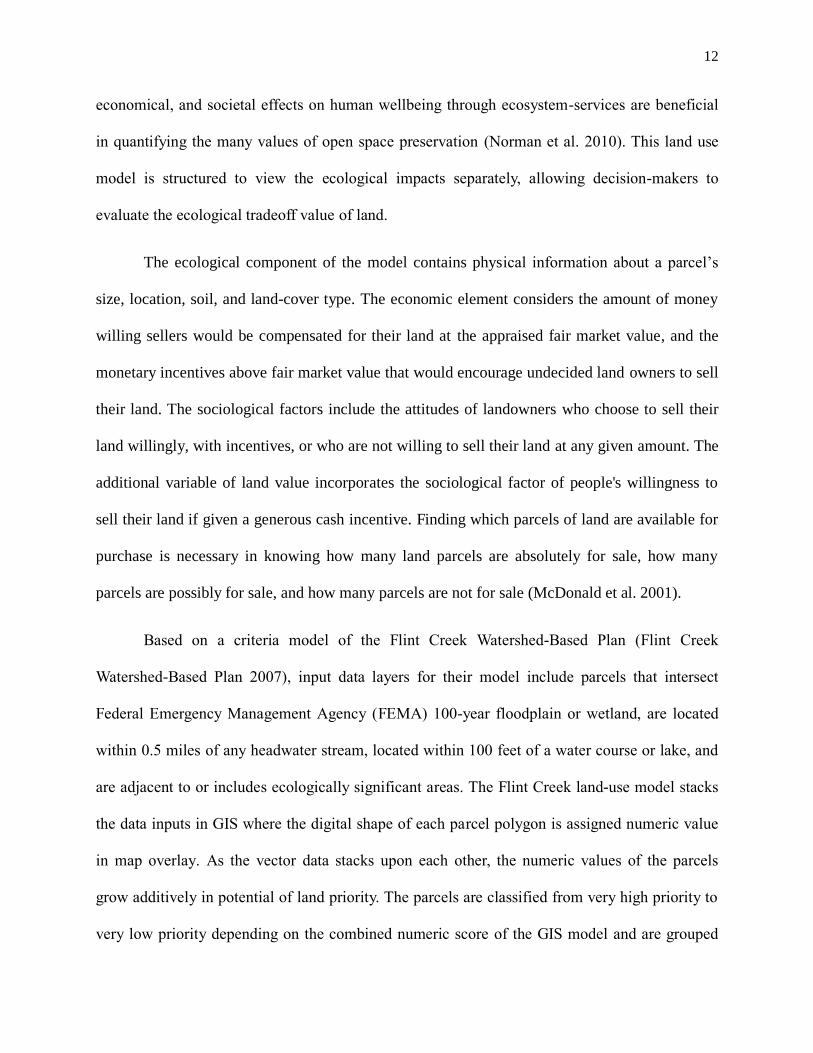
Based on a criteria model of the Flint Creek Watershed-Based Plan (Flint Creek

Watershed-Based Plan 2007), input data layers for their model include parcels that intersect

Federal Emergency Management Agency (FEMA) 100-year floodplain or wetland, are located

within 0.5 miles of any headwater stream, located within 100 feet of a water course or lake, and

are adjacent to or includes ecologically significant areas. The Flint Creek land-use model stacks

the data inputs in GIS where the digital shape of each parcel polygon is assigned numeric value

in map overlay. As the vector data stacks upon each other, the numeric values of the parcels

grow additively in potential of land priority. The parcels are classified from very high priority to

very low priority depending on the combined numeric score of the GIS model and are grouped

13

according to its applicability toward meeting the project goals. The MOSA model is similar in its

criteria ranking structure; but rather uses 150 square meter raster grid overlay in the weighted

sum tool where multiple inputs are stacked upon one another producing a final numeric pixel

value representing the natural values of a given parcel. The benefit of raster data is calculating

zonal statistics per parcel and per sample area where the mean value is classified by resource

richness.

In 2006, the town of Stonington, Connecticut adopted a similar model while prioritizing

land for open space acquisition (Gibbons 2011). Like the City of Boulder, Stonington’s primary

goals of open space conservation include protecting wildlife habitats, enhancing biodiversity,

maintaining farm land, serving aesthetic purposes, providing recreational opportunities,

preserving community character, and increasing contiguity between existing open space parcels.

The Conservation Commission established a list of criteria using GIS data layers to evaluate

individual parcels of undeveloped land. The GIS mapping allows planners to view the parcels

spatially, relative to the town’s natural resources and man-made features, such as roads and

subdivisions. The Stonington model omits any parcel smaller than thirty-five acres because they

deem it insignificant to wildlife. The MOSA land-use model omits subdivision parcels that are

already zoned for housing development yet considers every private parcel in the sample area as a

potential open space connection.

Another land-use model is discussed in the Wake County Open Space Plan where city

planners use GIS to overlay separate layers of information to reveal patterns of interrelated

landscape features (Open Space Prioritization Process of Wake County 2006). Once spatial

relationships are determined and patterns revealed, decisions can be made and implemented to

meet the goals defined by the city planners. The parcel methodology omits private parcels under

14

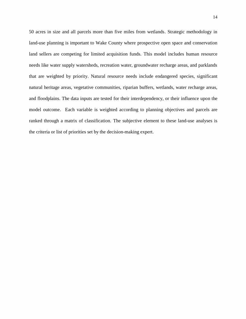
50 acres in size and all parcels more than five miles from wetlands. Strategic methodology in

land-use planning is important to Wake County where prospective open space and conservation

land sellers are competing for limited acquisition funds. This model includes human resource

needs like water supply watersheds, recreation water, groundwater recharge areas, and parklands

that are weighted by priority. Natural resource needs include endangered species, significant

natural heritage areas, vegetative communities, riparian buffers, wetlands, water recharge areas,

and floodplains. The data inputs are tested for their interdependency, or their influence upon the

model outcome. Each variable is weighted according to planning objectives and parcels are

ranked through a matrix of classification. The subjective element to these land-use analyses is

the criteria or list of priorities set by the decision-making expert.

15

CHAPTER THREE: METHODS OF MODELING OPEN SPACE ACQUISITION

(MOSA)

This chapter describes the process of building and authoring the Modeling Open Space

Acquisition (MOSA) land-use model. MOSA is built on the geo-processing Weighted Sum tool

in Esri ArcGIS as a technical, methodical approach that assists in classifying the ecological value

of land parcels. By testing the spatial data within the model, highly resourced land is identified

and targeted for open space acquisition. MOSA is specifically designed to provide supplemental

evidence in determining natural resource contributions of Boulder parcels.

3.1 Source Criteria in MOSA

The City of Boulder is governed by nine publicly elected city council members. Urban

planning depends on the professionals appointed by the City council, their priorities, planning

strategies, and political pressure placed on them. Every six years the city reviews the acquisition

plan of the open space administration. Open Space & Mountain Parks (OSMP) employs

environmental scientists, ecologists, and biologists who collect data and manage projects over

46,000 acres of public land. The City of Boulder is the first city in North America to designate

their own department for open space preservation (OSMP), aside from Parks & Recreation.

OSMP bases its goals and priorities through five Board of Trustees members who discuss current

affairs with staff and make recommendations to the Boulder City Council.

The year 2013-2019 acquisition process by OSMP presents a viable opportunity to use

multi-criteria decision analysis when planning open space acquisition by systematically applying

weighted criteria in a GIS model. The weight of each criterion is mostly decided upon by the

City of Boulder open space charter mission. The data layers used in MOSA are collected from

public sources and can adequately represent the criteria of the City of Boulder. MOSA was

16

accepted by the Boulder city council as a viable tool in real estate acquisition for OSMP in 2013

(City of Boulder Land Acquisition Report 2013).

Among the criteria for modeling the suitability index (i.e., the ecological richness) of a

parcel, property proximity is the most valuable contribution in open space acquisition because

the primary goal of the charter is to build connecting corridors of contiguous open space. The

riparian areas are second most important because wetlands support a plethora of prime habitats

that contribute a wide spectrum of ecological benefits. Open space land around the foothills of

Boulder supports vast species of flora and fauna that thrive at that biodiverse ecotone. Three

mountainous river systems merge into the western tributary of the Arkansas River: Boulder,

South Boulder, and Lefthand Creeks. The land within a mile or so of these river systems is

visibly richer in ecological resources. State and federal datasets with moderate details of wildlife

corridors are analyzed in MOSA. Recreational benefits from open space include public

connections to nature and increase public willingness to support it. When considering trail use,

the city council listens intently to public opinion, so recreation is weighted as moderately

important. Farms have cultural assets that improve their property value, and agriculture is

weighted as increasingly heavy in real estate acquisition because growing locally is a primary

goal for the City of Boulder.

17

3.2 Data Collection and Sources

Because private land has little or no available data, this thesis relies on public data

sources. The spatial area of the input must intersect the sample area: a one-mile buffer around the

four acquisition targets in the study area. MOSA takes multiple data inputs compiled by the

Colorado Natural Heritage Program (CNHP), the Colorado Ownership, Management, and

Protection (COMAP), the Colorado Parks and Wildlife (CPW) using the Natural Diversity

Information Source (NDIS) methodology, The National Map by United States Geological Survey

(USGS), the Federal Emergency Management Agency (FEMA), the Colorado Oil and Gas

Conservation Commission (COGCC), Boulder County Parcel/Assessor’s Data/GIS (BOCO), and

City of Boulder Open Space & Mountain Parks (OSMP). The ecological data are in 90 m and

150 m spatial resolutions, and includes metadata about data collection methodology from 2012.

These data must be re-projected from Lat/Long WGS 84 World Geographic Coordinate System

to a Projected Coordinate System for Northern Colorado (NAD 1983 HARN State Plane

Colorado North FIPS 0501 Feet). The MSOA data sources and their online addresses are listed in

Table 3.1. The public data sources are listed in the metadata Table 3.2.

Table 3.1: Public Data Sources that are used in MOSA

Sources: Online Address: Agency

BOCO

https://www.bouldercounty.org/gov/data/pages/gis

dldata.aspx Boulder County GIS Data

CNHP http://www.cnhp.colostate.edu/download/gis.asp Colorado Natural Heritage Program

COGCC

http://cogcc.state.co.us/Home/gismain.cfm

Colorado Oil and Gas Conservation

Commission

COMAP

http://www.nrel.colostate.edu/projects/comap/

Colorado Ownership Management

and Protection

CPW http://wildlife.state.co.us/Pages/Home.aspx Colorado Parks and Wildlife

FEMA

http://gis.fema.gov/ Federal Emergency Management

Agency

NDIS

http://ndis.nrel.colostate.edu/ftp/ Natural Diversity Information

Source

OSMP

https://bouldercolorado.gov/open-data Open Space & Mountain Parks GIS

data

USGS http://nhd.usgs.gov/ United States Geological Survey

18

Table 3.2: MOSA Data Sources and Metadata

Name of Data

Source

Name of Dataset Metadata

Boulder County GIS

Data

Significant Agriculture

Land

The Environmental Resources Element of the Boulder County

Comprehensive Plan provides more information in the mapping of the

Significant Agricultural Lands.

Boulder County GIS

Data

County Parcels Created from the Boulder County Parcel information layer digitized in parcel

fabric from legal descriptions using Coalition of Geospatial Organizations

(COGO) data.

Boulder County GIS

Data

Critical Wildlife

Habitat

3/9/1999 Polygon Attributes: Area - polygon area in square feet Perimeter -

polygon perimeter in feet - Wildlife Habitat

Boulder County GIS

Data

Significant Riparian

Corridors

Boulder County Comprehensive Plan; Boulder County Land-use Department,

Boulder, CO. 1986-1987.

Colorado Parks and

Wildlife NDIS

Abert’s Squirrel Species Activity Mapping (SAM), general scientific reference using 1:50,000

scale United States Geologic Survey county map sheets.

Colorado Parks and

Wildlife NDIS

Bald Eagle This is part of the Natural Diversity Information Source, drawing on map

overlays at 1:50,000 scale United States Geologic Survey county map sheets.

Colorado Parks and

Wildlife NDIS

Black Bear Fall Concentration Areas are defined as those parts of the overall range that

are occupied from August 15 until September 30 using 1:50,000 scale United

States Geologic Survey county map sheets.

Colorado Parks and

Wildlife NDIS

Elk Observed range of an elk population using 1:50,000 scale United States

Geologic Survey county map sheets.

Colorado Parks and

Wildlife NDIS

Great Blue Heron Foraging Areas for Great Blue Heron (Ardea herodias) in Colorado using

1:50,000 scale United States Geologic Survey county map sheets.

Colorado Parks and

Wildlife NDIS

Osprey Foraging Areas are defined as open water areas, typically associated with

larger rivers, lakes and reservoirs with abundant fish populations.

Colorado Parks and

Wildlife NDIS

Peregrine Nesting Areas for Peregrine Falcons in Colorado as defined by an area which

includes good nesting sites and contains one or more active or inactive nest

locations and include a 2 mile buffer surrounding the cliffs.

Colorado Parks and

Wildlife NDIS

Wild Turkey Overall winter range is defined as that part of the overall range where 90% of

the individuals are located from 11/1 to 4/1.

Open Space and

Mountain Parks

Habitat Conservation

Area

Management designations areas around the City of Boulder OSMP lands

according to the 2009 Visitor Master Plan. OSMP Property Property polygons for City of Boulder Open Space & Mountain Parks as

COGO defined from legal property descriptions.

OSMP Potential Areas of

Contiguity

Digitized polygons around the city of Boulder as identified in the Boulder

Valley Comprehensive Plan.

OSMP City Limits Created from the city parcel data layer by query of city limit boundary.

COMAP Public and Private

Land

Public and private agencies donate their GIS data and it is collaborated into

the COMaP dataset for distribution.

FEMA FEMA Floodplain FEMA: Data included represents Final Flood Insurance Rate Map (FIRM)

data that has been published as effective FIRM or DFIRM information.

COGCC Oil and Gas Wells The directional map layers are created using data supplied in the directional

surveys. .

USGS Hydrology for

Colorado

The NHD is the surface water component of The National Map. It contains

features such as lakes, ponds, streams, rivers, canals, dams and stream gages.

CNHP Potential

Conservation Areas

of Vegetation for

Boulder County

CNHP’s biologists work throughout Colorado to document critical biological

resources in Boulder County

19

3.3 Modeling Open Space Acquisition Methodology

This study provides a data driven analysis for determining resource-rich locations for

potential land acquisition. With the city of Boulder, CO in mind, this thesis authors the MOSA

land use model as a potential tool for the Open Space and Mountain Parks real estate division as

a supplemental evaluation tool in determining a suitable parcel to purchase for open space. The

original MOSA process incorporated one large model that became quite unmanageable. The

MOSA model was then broken into nine smaller sub-set models to process the data inputs

quickly and analyze the reliability of the model components. The logic behind the MOSA

structure is built upon fundamental land use prioritization methods using the goals of Boulder

and expert opinion from staff as a guideline of criteria. The top eight ecological priorities of

Boulder are represented in eight GIS models. This thesis builds, MOSA using the conflation of

eight class models plus one parcel model to generate raster data layers of various pixel numeric

values and score parcels. This list defines the terminologies used to explain MOSA:

Each class model in MOSA has a class weight defined by experts.

Each class model has multiple source inputs and converted into raster data.

Each source input has a source weight defined by experts.

Each model generates source weighted pixels of 150 square feet.

The source priority is the source weight multiplied by the source value per pixel.

The class priority is the class weight multiplied by the sum of the source priorities.

The suitability index is the sum of source priorities pixels averaged per parcel.

20

These eight class models in MOSA represent riparian corridors that support flora and

fauna, keystone wildlife species, oil and gas wells, historical sites, recreational areas of interest,

agricultural sustainability, vegetative quality, and parcel proximity in multiple criteria map

overlay. Each class model is a topic of consideration and contains multiple source models. For

example, the wildlife class model has ten inputs of species (i.e., ten source values) where each

species is ranked by their endangered criteria and their significance as a keystone species. The

vegetation model on the other hand has one input and consists of four classifications of

ecological importance. Each class model output enters the final weighted sum by their class

weight outlined by the expert opinion of the City of Boulder Land Acquisition Report (2013).

The City of Boulder Charter Purposes indicates the goals and criterion of city planners.

Separate class models maintain data manageability and controlled sensitivity screening.

Each class model follows a unique weighting strategy created by the experts to generate both the

class and source weights, which are defined by qualified staff, spatial analysis and reasoning,

popular vote, or city planning priorities and derivatives (Janssen 2001). Compiling available data

and applying weighted sum values in land-use modeling targets hot spots of natural resources,

thus assisting the decision-making process for land acquisition.

Using the class and source models, MOSA labels each pixel within the study area from

priorities 1 (low) to 9 (high). Each parcel in the study area is given a suitability index, which can

be interpreted as S for suitability index of a parcel, n as the total number of pixels in a parcel, and

X as the sum of source priorities (Riad et al. 2011). S is the suitability index, or average of the

combined source weighted priorities per parcel. The value of each raster pixel, X, is derived from

the weighted sum tool by the source model methodology in MOSA (Equation 3.1).

21

In Equation 3.1, W is wildlife, R is riparian corridor, E is oil and gas wells, C is cultural,

T is recreation and trail connections, A is agriculture, V is vegetation, and Q is property

proximity and size. The source weights, Pw...Pp, are based on the values of the elected leadership

of the City of Boulder (Table 3.3). The source priorities, W ...P, are generated by each of the

source models separately (described in Sections 3.3.2 to 3.3.9). Depending on the number of data

inputs, or priority criterion set by city planners, additional class or source models can be added.

For example, the current MOSA uses eight models, but if the City of Boulder wants to add a

ninth transportation factor, an additional class model named “Roads” would weigh the factors

Proad and includes sources such as distance to highways, byways, or bus stops. The following

priorities are based upon the published Charter Statement of the City of Boulder Open Space and

Mountain Parks. In 2013 Boulder city council approved MOSA as a tool in parcel selection. This

documentation is available on the OSMP website (City of Boulder Land Acquisition Report).

The MOSA land-use model methodology is detailed in the following sections with

explanation of each class model. Open source data is collected from responsible sources, clipped

to the boundaries of the defined sample areas, and converted into a raster grid cell through binary

values of presence or absence. Presence is represented by the number 1 and absence is given a 0

and removed from the dataset. The pixel values of 1 for presence are reclassified according to

the data input’s source weight. All data input raster cells overlay in the final weighted sum tool

where each is assigned its hierarchical significance called its class weight from levels 2-9. The

final dataset represents the suitability index of each parcel among the sample areas classified into

nine bins of ecological importance.

Equation 3.1: MOSA Class Priority

𝑋 = (𝑃𝑤 ×𝑊 + 𝑃𝑅 × 𝑅 + 𝑃𝐸 × 𝐸 + 𝑃𝐶 × 𝐶 + 𝑃𝑇 × 𝑇 + 𝑃𝐴 × 𝐴

+ 𝑃𝑉 × 𝑉 + 𝑃𝑞 × 𝑄 )

22

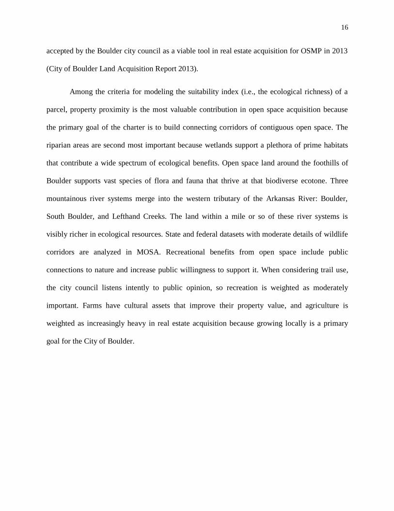
3.3.1 Parcel Selection Model

The parcel selection model finds target parcels outside of the city areas of Boulder and

within the sample areas, which are broken into four parts: Table Mountain, Accelerated

Acquisition Area, Mountain Parks, and Jefferson County Partnership. The parcel data of Boulder

and Jefferson counties are used to identify parcels that are publicly owned or annexed for

building development. The vector shapefiles of public lands are erased from the Boulder County

data layer. The private parcels remaining are clipped to the sample areas and the city limits are

removed (Figure 3.1). The existing private parcels (Figure 3.2) become tagged as potential open

space acquisition sites and are classified by priority in the final MOSA weighted sum analysis.

Table 3.3: City Council Priority Criterion by Rank Order

Data Layer Input Pixel Value

for Presence Reclassified Model Criteria Min

Pixel Value

Max Pixel Value

OSMP Land Distance in

Feet 1-9 Proximity 9 9 324 Habitat Conservation Areas

Boulder City Limits

OSMP Parcel size Size in Acres

Significant Riparian Corridors

1

8

Riparian 8 32 64 Hydrology 4

Wetlands 6

Oil and Gas Wells 1 7 Oil 7 49 98

Bald Eagle Nest Sites

1

9

Wildlife 6 12 54

Preble's Jumping Mouse 9

Critical Wildlife Habitat 9

Peregrine Nesting Area 8

Osprey Nesting Area 7

Great Blue Heron Nesting Area 6

Elk Migration Corridor 5

Wild Turkey 4

Abert's Squirrel 3

Black Bear Fall Concentration 2

Recreation 1 5 Recreation 5 25 25

Significant Agricultural Land 1-4 1-4 Agriculture 4 4 16

Potential Conservation Areas 1-3 1-3 Vegetation 3 3 9

Historical Sites 1 2 Historical 2 4 12

23

Fig

ure

3.1

: P

riv

ate

Par

cel

Sel

ecti

on

Mod

el

24

Figure 3.2: The Available Land within the Priority Areas of Boulder, CO

25

3.3.2 Wildlife Model

Ecological criteria in MOSA are suited for hierarchical structures where prime habitats

are ranked by importance according to conservation status assigned by Colorado Parks &

Wildlife. Multiple public data sets are available from NDIS and BOCO sources. Spatial layers

are selected if they meet the criteria of intersecting any of the four sample areas. The foraging

and nesting areas, or the winter and overall ranges, are merged per species. A numeric field is

calculated as 1 for presence of a species. The vector data are converted into raster cells and then

weighted by source weights (Table 3.4). The raster data enters the weighted sum geo-processing

tool and each species is ranked by its relative importance and level of threat on a scale of 2-9.

The weighted sum tool multiplies the raster cell value by the given priority ranking. The layers

of input are then summed per pixel and averaged within the parcel boundaries.

Table 3.4: Wildlife Source Weights in MOSA on a scale of 1-9

Species Source Weights

Bald Eagle 9

Preble’s Jumping mouse 9

Critical Habitat 9

Peregrine Falcon 8

Osprey 7

Great Blue Heron 6

Elk Migration Corridor 5

Wild Turkey 4

Abert’s Squirrel 3

Black Bear 2

26

The species’ rankings (source weights) come from the OSMP ecological staff (Heather

Swanson, PhD, OSMP Wildlife Ecologist at swansonh@bouldercolorado.gov and Eric Stone,

OSMP Resource Information Division Manager at stonee@bouldercolorado.gov). The weights

are based on their analysis of the Boulder County listing of species of state concern (Hallock

2010). Additional analysis considers the recommendations of the endangerment list provided by

Colorado Parks and Wildlife, which classifies species by State Concern, State Endangerment,

State Threatened, and Federally Endangered or Federally Threatened according to the US Fish

and Wildlife Service. These raster source data enter the final weighted sum with a class weight

of 6 (Table 3.3). Figure 3.3 shows the wildlife model species and their hierarchical rankings of

importance called their source weights. The minimum pixel value for the wildlife output is 12,

where the lowest Black Bear present is a reclassified pixel with a source weight of 2 multiplied

by its class criteria 6. The maximum pixel value is 54, where the highest priority of Bald Eagle

or Peble’s Jumping Mouse present is a reclassified pixel with a source weight of 9 multiplied by

its class criteria 6. The wildlife model could produce pixels that are higher than 54 in locations

where mulitple species overlap in common space. This model output represents the wildlife

contribution in the land use evaluation.

27

Figure 3.3: Wildlife Model in MOSA

28

3.3.3 Riparian Model

The digital layers for the riparian model in MOSA include Boulder County wetlands and

significant riparian corridors, and OSMP hydrology data. The hydrology linear features are

buffered by 150 feet, as identified by the Town Stonington, CT in their land use model to include

variations of hydrologic stream flow. Buffering serves the purpose of converting the line data

into polygon form to match the other data types. The two wetlands vector layers are merged into

one dataset. The sources used in the riparian model are riparian, hydrology, and critical habitat

data, which are converted into raster by the numeric value of 1 for presence. The riparian data is

placed into a weighted sum tool that ranks the data by factors of importance (i.e., the source

weights). The wetlands are weighted by 6, the critical habitat by 8, and the hydrology by 4. The

riparian input is given a class weight of 8 in the final analysis (Table 3.5) so the minimum pixel

value for the riparian output is 32 and the maximum pixel value is 64. Figure 3.4 is the riparian

model in detail while Table 3.5 describes the data source, the conflation procedure, and the

source weights of the pixels.

Table 3.5: Riparian Data Structure in MOSA

Data Source Data Input Process Data Type Raster Value Source

Weights

BOCO Riparian

Corridor

Polygon 1 or 0 8

USGS Hydrology Buffer 150

Ft

Line to Polygon 1 or 0 4

FEMA Floodplain Polygon 1 or 0 6

29

3.3.4 Oil and Gas Model

The data layers of the oil and gas model include the point locations of oil well sites in

Boulder County as provided by the Colorado Oil and Gas Conservation Commission. The points

are buffered by 200 feet around the geographic location to convert the point data into polygons.

A numeric field is added to the attribute table and calculated 1 for presence. Zero values are

removed from the dataset. The polygon is converted into raster pixels and then reclassified from

1 to its source weight of 7 (Table 3.3). The minimum pixel value of the oil output is 49 (source

weight 7 times class weight 7), and maximum pixel value is 98 (two oil wells located within one

pixel). Figure 3.5 displays the oil class model in detail.

Figure 3.5: Oil and Gas Model in MOSA

Figure 3.4: Riparian Model in MOSA

30

3.3.5 Cultural Model

The data layers of the cultural model include the point locations of historical sites in

Boulder County. The points are buffered by 200 feet to allow for the area around the geographic

location to convert the point data into polygons. A numeric field is added to the attribute table

and calculated 1 for presence. The vector data is then converted into raster pixel cells based on

this field of presence. The raster is reclassified from 1 as present to its source weight of 2 (Table

3.3). The minimum pixel value for the cultural output is 4 (source weight 2 times class weight 2),

and the maximum pixel value is 12 (three cultural sites located within one pixel). Figure 3.6

displays the cultural class model in detail.

3.3.6 Recreation Model

Ecologists agree that protecting isolated natural areas is only a beginning to functional

urban design. When connecting metropolitan areas there are two primary objectives, the first is

ecological and the second is human (Forman 1995). Sustainability goals of Boulder include the

connectivity of regional and local trails. In the MOSA model the data layers include three inputs:

digitized areas of trail connections identified by the City of Boulder City Council in 2012, areas

agreed upon in the Boulder Valley Comprehensive Plan, and areas of connections between trails

less than two miles apart that represent potential contiguity. The three inputs are merged and

Figure 3.6: Cultural Model in MOSA

31

converted into raster data with a binary value of 1 for presence or 0 for absence. The raster pixels

are reclassified from 1 as present to its source weight of 5 (Table 3.3). The minimum pixel value

for the recreation output is 5 and the maximum pixel value is 25, (presence source weight of 5

multiplied by its class weight of 5). Figure 3.7 displays the recreation model in detail.

3.3.7 Agriculture Model

The data input for the agriculture model is from the Boulder County website and

represents four categories of significant agricultural land in Boulder County: 4 as very significant

to 1 as low significance. A sustainable agricultural economy is an integral part of Boulder

County’s long range planning. The vector layer is converted into raster pixel data based on this

classification of 1-4. The minimum pixel value for the agriculture output is 4 and the maximum

pixel value is 16 (source weight

1-4 times class weight 4). Figure

3.8 displays the agriculture class

model in detail.

Figure 3.7: Recreation Model in MOSA

Figure 3.8: Agriculture Model in MOSA

32

3.3.8 Vegetation Model

The Colorado Natural Heritage Program sponsored by Colorado State University

provides the digital data for potential conservation areas in Colorado in three classifications: 3

being the most critical to 1 being somewhat critical. The vector polygons are converted into

raster pixel data by its source weight of 1-3 and then multiplied by its class weight of 3 (Table

3.3). The minimal pixel value

from the vegetation output is 3

and the maximum pixel value is

9. The vegetation class model is

detailed in Figure 3.9.

3.3.9 Proximity Model

The proximity model consists of near distance and size measurements of available

parcels. The near tool measures the direct distance from the parcel centroid to its nearest

neighboring polygon (parcel). The OSMP property data layer is used to calculate distance in feet

from each available parcel to the nearest OSMP land, OSMP habitat conservation area, and to

the centroid of Boulder city limits. The area of each available parcel is calculated in square feet.

These three proximity distance inputs and one parcel size input are reclassified on a scale from 1

to 9, nine as the closest or largest parcels and one as the furthest or smallest parcels. The

polygons are converted to pixels based on their 1 to 9 nearness and size classes. The four

proximity inputs enter the weighted sum with a source weight of 1 so that they retain their 1-9

classifications. Figure 3.10 details the proximity model and its three near distance and one size

reclassifications.

Figure 3.9: Vegetation Model in MOSA

33

Fig

ure 3

.10:

Pro

xim

ity M

odel

in M

OS

A

34

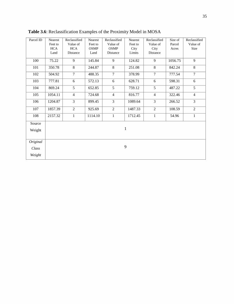
Table 3.6 samples the MOSA reclassification methods where the distance and area in feet

are converted into integers and reclassified from 1-9. The pixel value of the raster data becomes

nine when closest in feet to the selected neighboring parcels and lessens to one when furthest

away. The area of each parcel is measured in acres and then reclassified into sizes from 1-9. The

largest bin of property size is reclassified as nine, moving downward to the smallest property size

as one. The three proximity inputs and the parcel size input enter the weighted sum tool where

they are layered and multiplied by a source weight of 1. This proximity layer enters the final

class model as the proximity input. The proximity input is given the criterion ranking of 9, as

noted in Table 3.6 as “Original Class Weight”. This methodology assigns heterogeneous pixel

weights to different parcel proximity criterion, recognizing the diverse aspects of spatial options

that contribute toward decision objectives (Ligmann-Zielinska 2012). The minimum pixel value

of the proximity input is 9 (least source weight 1 times the four data inputs, times its class weight

9), and the maximum pixel value is 324 (max source weight 9 times the four data inputs, times

its class priority 9). The mean pixel value per parcel is calculated using the zonal statistics

method. The average parcel pixel value, called its suitability index, is divided into nine natural

breaks among the sample area using Jenks classification method. The parcel suitability indices

range from 46-1,672 and are detailed in Table 3.7 on page 38.

35

Table 3.6: Reclassification Examples of the Proximity Model in MOSA

Parcel ID Nearest

Feet to

HCA

Land

Reclassified

Value of

HCA

Distance

Nearest

Feet to

OSMP

Land

Reclassified

Value of

OSMP

Distance

Nearest

Feet to

City

Limits

Reclassified

Value of

City

Distance

Size of

Parcel

Acres

Reclassified

Value of

Size

100 75.22 9 145.84 9 124.82 9 1056.75 9

101 350.78 8 244.87 8 251.08 8 842.24 8

102 504.92 7 488.35 7 378.99 7 777.54 7

103 777.81 6 572.13 6 628.71 6 598.31 6

104 869.24 5 652.85 5 759.12 5 487.22 5

105 1054.11 4 724.68 4 816.77 4 322.46 4

106 1204.87 3 899.45 3 1089.64 3 266.52 3

107 1857.39 2 925.69 2 1487.33 2 108.59 2

108 2157.32 1 1114.10 1 1712.45 1 54.96 1

Source

Weight

1

Original

Class

Weight

9

36

3.3.10 Classification Methods

In the following paragraphs, Jenks Natural Breaks Optimization method classifies the

MOSA pixels within the study area by breaking classes between large gaps of ecologic values. In

comparison, Quantile classification predefines the nine classes used and ranks the pixel value by

placing an equal number of observations into each class.

As seen in Figure 3.11, more pixels in the sample area are showing as ecologically rich

because the classification bins are filled with an equal number of entries. The advantage to using

Quantile class breaks is that each

pixel is represented equally in

the final map, but its

disadvantage is that it leaves

large gaps between levels of

observations. In some cases, one

classification interval is

overrepresented. For this reason,

Quantile classification is not

used in MOSA. The clustering of

ecologically rich land is better

represented by the Jenks

classification method.

Figure 3.11: Quantile Classification Method upon Pixels

37

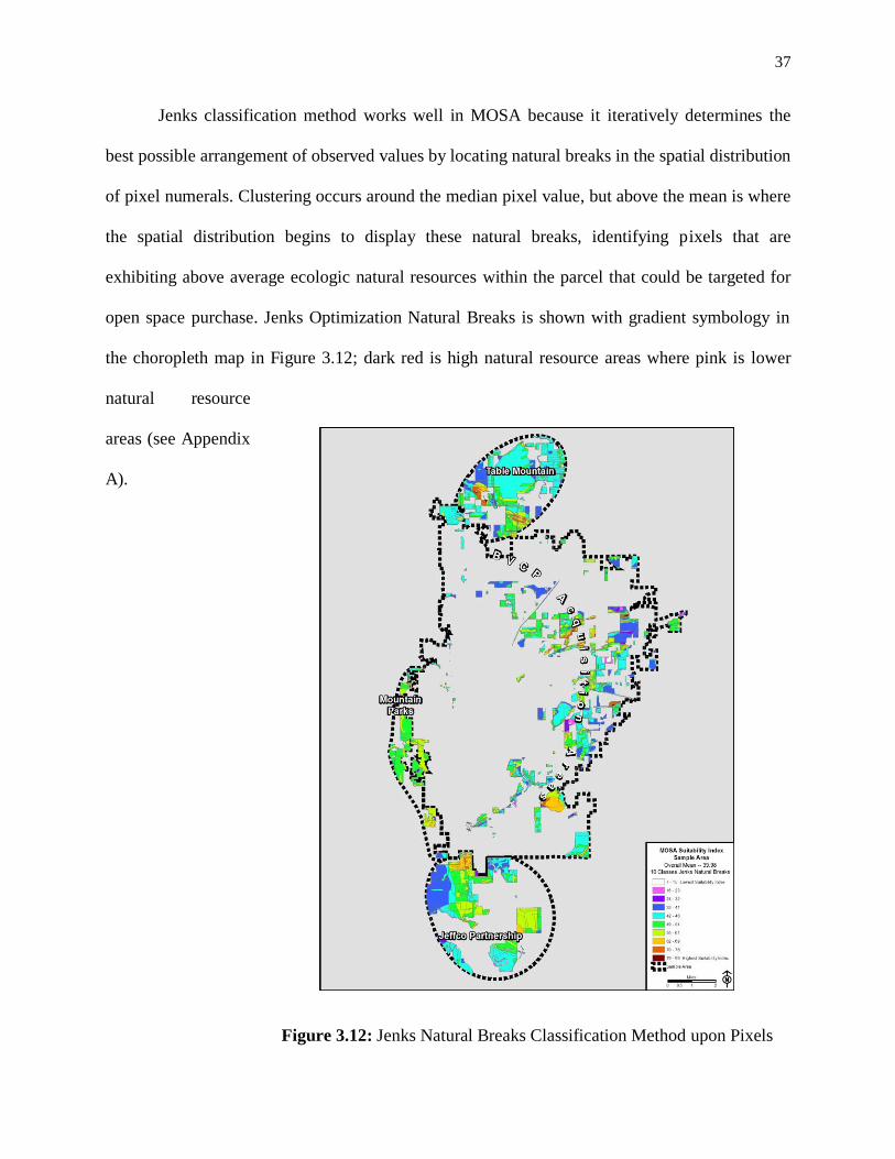
Jenks classification method works well in MOSA because it iteratively determines the

best possible arrangement of observed values by locating natural breaks in the spatial distribution

of pixel numerals. Clustering occurs around the median pixel value, but above the mean is where

the spatial distribution begins to display these natural breaks, identifying pixels that are

exhibiting above average ecologic natural resources within the parcel that could be targeted for

open space purchase. Jenks Optimization Natural Breaks is shown with gradient symbology in

the choropleth map in Figure 3.12; dark red is high natural resource areas where pink is lower

natural resource

areas (see Appendix

A).

Figure 3.12: Jenks Natural Breaks Classification Method upon Pixels

38

3.3.11 Final Weighted Criteria Model

The final weighted analysis is performed by multiplying the sum of stacked pixel values

from each sub-set model by its class priorities defined by the expert decision makers. The

absolute pixel values are averaged within the parcel boundary and are called the parcel’s

suitability index. Each parcel within the study area is classified into one of nine bins of

suitability indices, or their ecological contribution, according to Jenks Natural Breaks

classification method. The parcels in the top four levels are selected for further analysis.

The numeric quantity of the pixel represents the quality of land ecologically, ideally

representing the parcel’s environmental service toward human health. The final output is masked

or extracted by the available land parcel layer (created from the parcel selection model, Figure

3.1) and individual parcel suitability index is calculated using Equation 3.1. Figure 3.13 displays

the class models feeding into the final weighted sum tool of MOSA and weighted according to

the criterion set by the expert, or city planners of Table 3.3. The minimum pixel value for the

final weighted sum output is 46 and the maximum pixel value is 1,672 as graphed in Figure 3.14.

The nine classification bins of suitability indices among the available parcels are listed in Table

3.7.

Table 3.7 Original MOSA Parcel Suitability Indices using Jenks Classification

Parcel Suitability Index Pixel Value

Lowest 46-331

332-530

531-689

690-818

Mean 819-946

947-1078

1079-1200

1201-1398

Highest 1399-1672

39

Fig

ure 3

.13

: T

he

Fin

al W

eighte

d C

lass

Cri

teri

a M

odel

in M

OS

A

40

Figure 3.14 shows the zonal statistics per sample area using the Jenks Natural Breaks

classification method. The Jefferson County Partnership area scored the overall highest

maximum range of property ecologic values. The BVCP area was the second highest scoring,

Table Mountain area was the third largest range, and the Mountain Parks area scored fourth

among the sample areas. The highest average mean of ecological resources is found in the Table

Mountain sample area. Parcels in the Jefferson County Partnership have the greatest suitability

index with the greatest range, most likely due to its wildlife corridor, multiple eagle nests,

intersecting riparian areas, and large parcels contiguous to existing open space.

Figure 3.14: Zonal Statistics and Distribution of MOSA Data by Sample Area

1672

1523

1581

1900

1700

1500

1300

1100

700

500

900

300

100

1268 1206

1626

1477

1532

246

490

684

84

62

46

46

49

41

Figure 3.15 is an example of a useful form showing how the results of MOSA can be

combined with other data to aid the parcel acquisition decision-making process. The parcels in

the top four levels from the Jenks Natural Breaks Optimization are targeted and compared to its

economic demand. The open space parcel rating sheet is a clean and convenient way of

quantifying the carrying capacity of a particular parcel while weighing the pros and cons of

acquiring it.

Figure 3.15: Example Open Space Parcel Rating Sheet

Parcel Name: _______________________________________________________________________

Parcel Number: _____________________________________________________________________

Date of Analysis: ___________________________________________________________________

Acquisition Area: ___________________________________________________________________

Suitability Index: _________________

Priority Ranking: _________________

Sub-Class Ranking by Factor:

Parcel

ID

Wildlife Riparian Oil/

Gas

Historical Recreation Agriculture Vegetation Proximity Suitability

Index

100 64 52 18 12 47 22 30 84 329

Overall Ranking:

Parcel

ID

Suitability

Index

Zonal

Statistics

Ranking

Market

Value of

Parcel

Asking Price

of Parcel

Incentives for

Parcel

Purchase

Total Price

of Parcel

Decision

100 329 High 500,000 550,000 $10,000 560,000 Yes

Notes:

Zonal Statistics Criteria:

This classification is the range of mean suitability index among the acquisition areas

Priority Accelerated Acquisition Area Table Mountain Mountain Backdrop Jefferson County Partnership

High

Medium

Low

42

CHAPTER FOUR: MOSA RESULTS

In this chapter, section 4.1 presents the experiment results using MOSA for identifying potential

private parcels for open space acquisition based on the original theoretical criterion from the City

of Boulder. Private parcels with the greatest ecologic resource are determined by the Jenks

Natural Breaks classification method of the average pixel value per parcel within the study area.

This section also presents the recommendation of an adjusted criterion ranking that improves the

efficacy of the final output.

4.1 MOSA Results in Detail

Using the original criterion provided by the City of Boulder this study identified 1,024

private parcels within the four sample areas that display potential for open space acquisition.

MOSA classifies the ecological richness of these private parcels by averaging the pixel values

within each parcel. The parcel average ranks its suitability index for open space conservation.

The averages are separated into nine classifications using Jenks Natural Breaks; one being the

lowest suitability index, and nine being the highest. The 415 parcels in the top four levels are

detected and further evaluated for potential open space acquisition. For the purpose of this thesis

the original analysis uses the criteria (i.e., both the source and class weights) set by a theoretical

City of Boulder council and results in clustered spatial distributions throughout the sample areas.

43

Figure 4.1 displays the 415 targeted parcels within the combined sample areas that score

a suitability index of 6, 7, 8, and 9 from the Jenks classification in the original land-use weighted

criterion. MOSA found these parcels ecologically desirable with above average natural capital

and could become a top priority for open space acquisition. These results suggest reasons for

spatial clustering among the

MOSA output that is not

occurring randomly, but

because the parcels possess, or

are contiguous to ecologically

rich land. These private

parcels identified as the four

top classes in Jenks deserve

recognition, investigation, and

potential open space

acquisition. These findings

serve as explanatory evidence

for city planners when

comparing ecological and

economic land values for the

intent of parcel prioritization

for open space land.

Figure 4.1: MOSA Targeted Parcel Spatial distribution of

parcel suitability indices using the original criterion

from the Top Four Jenks Classifications

44

Subjectivity is inherent in any expert-based model and should be recognized as potential

for creating model bias (Goodchild 1998). Original theoretical criteria set by the City of Boulder

Charter Purpose (Table 3.3), prioritizes parcel proximity as the top ranking of class weight 9, but

this weight is much too heavy in the final criteria. The parcel proximity pixel value inflated the

final dataset and dissipated the other model inputs. Without the proximity input, the range of

suitability indices for parcels within the study areas ranged between 4 and 184. With the

proximity input included the suitability indices raised from 4 to 1,817. The proximity input was

close to ten times the volume of the other data inputs when summed in the final criteria ranking.

This bloating of suitability indices indicate bias in the MOSA model where the proximity input

was negating the influence of the other seven datasets. The influence of a parcel’s proximity to

other ecologically rich land should be reduced so that it is closer in weight to the other data

inputs.

One way to reduce the proximity output is to diminish the source weights in the proximity

model by a tenth of their original level. In the adjusted theoretical criteria the first proximity

nearness parameters is assigned the source weights of .5 to habitat conservation areas instead of

5, .4 to existing open space land instead of 4, .2 to city center instead of 2, and the size of the

parcel is weighted by .3 instead of 3 (Table 3.6). The pixel value is much smaller in this model

scenario and reduces the overwhelming presence of the proximity model by one tenth in the final

weighted sum. After sensitivity testing was performed upon each data input by iterating its class

weights within the weighted sum tool, it is recognized that the datasets are most proportionate in

relation to each other when reducing the mass and class priority of the proximity model. The

adjusted results reflect the class weight of the proximity model as level 2, cultural as level 3,

45

vegetation as level 4, agriculture as level 5, recreation as level 6, wildlife as level 7, oil as level

8, and riparian as level 9.

The following paragraphs detail the results of the MOSA original criterion analysis against

the adjusted criterion analysis. The spatial distribution of the original MOSA class and source

weights is clustered in the above average classification as shown in Figure 4.2. The proximity

input is classifying more parcels as ecologically rich the greater the weight criterion, which

means bias in the model parameters because not every data input is contributing effectively in

the weighted results. The spatial distribution of the adjusted weighted criteria after the sensitivity

analysis had fewer parcel clusters in the higher classifications and is more bell-shaped curved

approximating normal distribution.

Suitability Index

46

The differences between the original model criteria and the adjusted criteria are displayed in

Figure 4.3. The selected parcels are chosen from the top four classes of Jenks. In the original

model there are 415 parcels that are classified as having above average ecological resource, but

the sensitivity testing suggests that this model outcome is biased toward the proximity model

parameters and fails to adequately represent the underlying data layers. After adjusting the class

and source weights of the proximity model, the number of above average parcels increases to

457, and they were different parcels than from the original outcome. This could be from the other

ecological datasets becoming meaningful in the final weighted distribution. The output from the

Figure 4.2: The Spatial Distribution Comparison of Parcel Suitability Indices

Spatial distribution of parcel suitability indices using the original criterion

Spatial distribution of parcel suitability indices using the adjusted criterion

47

adjusted model is more representative of the full spectrum of data and is best suited for this

weighted criteria analysis (see Appendices B and C).

Figure 4.3: Parcel Criterion Comparison

Adjusted weighted criterion results

Adjusted weighted criterion results

Original weighted criterion results

Adjusted weighted criterion results

48

CHAPTER FIVE: FUTURE WORK AND CLOSING DISCUSSION

Future model modifications and spatial autocorrelation are discussed in section 5.1, while section

5.2 concludes this thesis by discussing the multiple benefits of land-use modeling for open space

prioritization.

5.1 Future Model Considerations and Limitations

An additional function of the MOSA model includes dynamic interactions between

conditional responses of model elements in reaction to their environment. For example, this land

use model considers wildlife habitat and recreation corridor in the weighted sum evaluation as

presence or absence, when in actuality the wildlife highly suitable habitat may decrease with the

presence of trails or human impact. The more sophisticated land-use model would respond to the

presence of impacting anthropogenic factors like roads, noise, or traffic volume and would react

negatively according to the scale of impact. The resulting product of each pixel would vary

dynamically and stochastically as various factors interact within variations of model criteria. For

example, this would include buffering trails and roads by a certain threshold of impact and then

building an algorithm that estimates a parameter of stress-response. The area of impact is found

in the intersection of the trail or road buffer overlapping with other ecologic inputs. These

effected pixels within the impact area would lessen in value stochastically (Wu et al, 2007).

A second consideration is that the model developed for this study does not consider the

parcel owner’s willingness to sell their land. Veto threshold survey data collected over the

sample area would include the parcel owner’s willingness to sell their land at market value,

49

above market value, or not willing to sell their land at any given price and only the available

parcels would be considered in the final analysis.

Overall results indicate the proximity input class model is rather heavy for the overall

weighted sum and could be reduced by a tenth to equal the lesser inputs. An additional parameter

to alleviate the overweighed proximity input is adding a near distance table for every class

model, to measure its location to existing open space land, habitat conservation area, and city

center. The value for each feature class would then be increased depending on its proximity to

the same feature class in other pixels. The existing proximity model measures near distance from

each parcel to existing open space, habitat conservation areas, and city center, and considers

parcel size, and then classified as 1-9 in the proximity model and given the criteria weight of 9.

Every ecological input could also be measured in nearness to existing open space land, habitat

conservation area, city center, and its size, and then reclassified as 1-9 in the final weighted sum

with the criteria weight for each input found in Table 3.3. For example, the size and location of

an existing riparian area in relation to habitat conservation areas could be classified in near

distance tables like the parcel proximity. This method would increase the pixel value of each

ecological input in the final weighted output with its presence and nearness classifications in the

criteria analysis so that potential scores on all measures would be more evenly weighted.

Subjectivity testing as mentioned in this thesis suggests the proximity model is sensitive

among the other inputs because of its spatial volume (spatial autocorrelation exists in other input

and is explained next in this section). It is recognized that the proximity model displays clustered

spatial distribution and is notably very influential to the land-use model prediction. These

clusters are lacking randomness and could be explained by the nearest neighbor likeliness among

50

ecologically rich areas like riparian wetlands, wildlife corridors, and the parcel proximity in

relation to existing open space land. The ecologically rich lands are most likely near river

systems or drainages where flora is present and wildlife has viable food and water sources. The

City of Boulder city council approved MOSA with the original criterion rankings where the

proximity model is the primary influence in the parcel classifications. This research suggests

modifying future analysis by the adjusted criterion levels so the eight ecological input datasets

are most equally considered in the final weighted sum suitability index.

Spatial autocorrelation measures the degree to which spatial clustering itself explains

change in dependent variable values. It is based on the idea that near subjects within the sampled

area are more likely to have similar values than are subjects further apart (Tobler 1970). When

spatial data display autocorrelation, it is possible, at least in part, to predict the pixel value at one

location based on the pixel value sampled from a nearby location. In the MOSA model

developed for this thesis, clustering patterns within the sampled area may be evident and may

often be due to the likeliness of nearby ecologic values. Autocorrelation can be explained by

dependent and independent responses to the variable’s surroundings. For example, a plant may

thrive in an area where its dependent soil, water, and air temperature are ideal for its survival.

This location is more likely to support an abundance of plant life than other areas that are less

ecologically suited. Wind speed may interact with the soil or air temperature disrupting the

reproductive cycle of the plant. The plant abundance variable is both dependently and

independently autocorrelated to itself under a given circumstance. Both influences result in

similar values of plant abundance or plant disparity each in close proximity and in distance.

51

In this land use criteria model, the pixel values on each measure may not be fully

independent of themselves or of their locations. In fact, it may be the case that the clustered

ecologically rich parcels in the top four classifications are displaying spatially autocorrelation.

For example, the further the parcels are from protected land, the less likely they will score well

for the ecologic contribution to their suitability index. The proximity variable is already over-

weighted in the model and it may be inherent in some of the ecological variables as well. This

may also be creating biased clusters of highly suitable parcels overly dependent upon nearness

and size parameters over other influences in the model and skewing the results. At the very least,

it is not possible to say that the weightings dictated for the model are being carried out with

precision. Further autocorrelation and statistical examination of this land use model would be

beneficial in testing its reliability to determine whether the highly suitable parcels remain

clustered after the proximity parameters and the influence of proximity itself are lessened in the

final weighted sum. The latter results could further explain consistently high suitable parcel

clusters near dependent ecologically rich riparian areas, wildlife corridors, river systems, and

trail connections even after the proximity criteria are reduced.

5.2 Closing Discussion

Scientific analysis of weighted criteria for open space acquisition requires modeling that

is adaptive with interchangeable data layers, functional with consistent results, and replicable for

others to adopt. The final weighted sum in this example of land use prioritization considers nine

class model criteria that are interchangeable and flexible as city planning priorities adapt over

time. This research model is adaptive because each input is contained within its own model and

data can interchange easily. It is functional because the model output serves as supplemental

evidence in prioritizing open space acquisition for ecological preservation, inherently improving

52

the intrinsic value of the community that it serves. It is also replicable because it is simple and

straightforward by design. The weighted criteria of a functional land-use model should be

interrogated through sensitivity testing. This is done stochastically or intentionally by generating

various model outputs based on iterated changes to the set criteria within the weighted sum tool.

The sensitivity testing will validate the strength and weakness of variable relationships and

expose model bias so adjustments can be allocated to the final model criteria. Given the effectual

association between land acquisition and the planning context, analysts should use land-use

models when examining future open space acquisitions (Gerber 2012). Often land is coveted for

its economic value, but ecological values are neglected due to a lack of information or concern

by city planners. In multi-criteria decision analysis, expert planners can vary their criteria

ranking by prioritizing the changing values of a community. Even when a community agrees on

supporting open space acquisition, strategic methods should be followed when choosing parcels

to preserve. Public ecological data is often coarse, but at least offers a glimpse of reality in

private areas where data is limited.

Open space can be defined as land that is not developed yet and provides a valued habitat

for humanity to coexist with its flora and fauna. It is the working landscape of forests, farms,

scenic byways, greenbelts, natural areas, and wetlands, each synergistically contributing to the

intricate web of ecological balance with minimal human impact. Open land can be acquired and

preserved for the well-being of current and future generations. It is the right and responsibility of

a given community to protect hedonic nature from anthropogenic affliction (Speth 2008). This is

done through a proactive public process, like voting for open space acquisition by using city

sales tax allocation. The open space land that is acquired and managed by a governing agency

53

can have above average ecological value and be stringently tested under the parameters of a

land-use model that quantifies the natural resources present.

In conclusion, this thesis creates, defines, and develops the Modeling Open Space

Acquisition, expert-based, multi-criteria, decision making model, to identify and quantify a

parcel’s ecological natural assets for the purpose of prioritizing private parcels and preserving

public open space. The priorities of city planners can be ranked by criteria in a GIS environment

to scientifically evaluate the carrying capacity of a given parcel prior to purchasing it. Evaluating

the ecologic potential of a parcel before acquiring it can eliminate the costly expense of

purchasing land that is low in ecological resources and requires costly restoration or extreme

management. Land use modeling is an important tool in detecting ideal areas for future open

space acquisition by modeling the spatial relationships between ecologically rich parcels and

their proximity to contiguous open space lands. Ecologically rich parcels can be investigated

more closely and become a top priority for the City of Boulder to acquire and preserve as open

space.

54

REFERENCES

Bento, A., D. Kaffine, and S. Franco. 2011. “The Value of Open Space: Evidence from Studies of

Nonmarket Benefits.” Resources for the Future January: 1-78.

Bockstael, N., R. Costanza, I. Strand, W. Boynton, K. Bell, and L. Wainger. 1995. “Ecological

Economic Modeling and Valuation of Ecosystems.”Ecological Economics 2:143-159.

Cheviron, B., Y. Le Bissonnais, S. J. Gumiere, J. F. Desprats, A. Couturier, F. Darboux, and D.

Raclot. 2011. “Comparative Sensitivity Analysis of Four Distributed Erosion Models.”

Water Resources Research 47:1-17.

City of Boulder Open Space and Mountain Parks. 2012. "Open Space and Mountain Parks

Acquisition Update 2013-2019." https://www-static.bouldercolorado.gov/docs/2013-

2019_OSMP_Acquisiton_Plan_Update-1-201308210851.pdf (accessed 12 August 2013).

Colorado Parks and Wildlife. 2012. "Colorado Parks and Wildlife Threatened and Endangered

List."

http://wildlife.state.co.us/WildlifeSpecies/SpeciesOfConcern/ThreatenedEndangeredList/

Pages/ListOfThreatenedAndEndangeredSpecies.aspx (accessed 25 January 2013).

Czech, B. 2001. "A Transdisciplinary Approach to Conservation Land Acquisition."

Conservation Biology 16:1488-1497.

Czech, B. 2009. “Ecological Economics.”Animal and Plant Productivity.” 4:222-265.

Chandio, I. A., A. N. Matori, D. U. Lawal, and S. Sabri. 2011. “GIS-Based Land Suitability

Analysis Using AHP for Public Parks Planning Larkana City.” Modern Applied Science

5:4:177-190.

Costanza, R., R. d'Arge, R. D. Groot, S. Farber, M. Grasso, B. Hannon, K. Limbur, and M. van

den Belt. 1997. “The Value of the World's Ecosystem Services and Natural

Capital.”Nature 387:253-259.

Crooks, A., C. Castle, and M. Batty. 2008. “Key Challenges in Agent-based Modelling for Geo-

spatial Simulation.”Computers, Environment and Urban Systems 32:417-430.

Dai, E., and S. Wu. 2005. “Modeling Change-Pattern-Value Dynamics on Land-use: An

Integrated GIS and Artificial Neural Networks Approach. “Environmental Management

36:579-591.

Erickson, D. 2012. “Transportation-Movement.” MetroGreen-Connecting Open Space in North

American Cities. Washington, DC, USA: Island Press. ISBN 1-55963-843-5.

Farber, S. C., D. Bradley, and R. Costanza. 2002. "Economic and ecological concepts for valuing

ecosystem services." Ecological Economics 41:375-392.

55

Flint Creek Watershed-Based Plan. 2010. "Open Space/Green infrastructure Parcel

Prioritization." http://flintcreekwatershed.org/watershed_plan.html (accessed 13

September 2013).

Friedman, S. D. 1990. Assessing the Value of Land Contributed to a Real Estate Joint-Venture

Development.” Real Estate Newletter, Winter: 7.

Gerber, J. D., and A. R. Rissman. 2012. "Land-conservation Strategies: the Dynamic

Relationship between Acquisition and Land-use Planning." Environment and Planning A

44:1836-1855.

Gergely, K., J. M. Scott, and D. Goble. 1997. “A New Direction for the US National Wildlife

Refuges: The National Wildlife Refuge System Improvement Act of 1997.” Natural

Areas Journal 20: 107-118.

Gibson, J. 2011. “Open Space Planning.” Cooperative Extension System - College of Agriculture

and Natural Resources: 1-16.

Gomez-Pompa, A., and A. Kaus. 1992. “Taming the Wilderness Myth.” BioScience 42:271-279.

Goodchild, M. F., S. Guoqing , and Y. Shiren. 1992. “Development and Test and an Error Model

for Categorical Data.” International Journal of Geographical Information Systems 6:87-

104.

Grimes, A., and A. Aitken. 2010. “Housing Supply, Land Costs and Price Adjustment”. Real

Estate Economics 38:325-353.

Hallock, D., and S. Jones. 2010. “Boulder County Avian Species of Special Concern.” Boulder

County Nature Series 1:1-36.

Ham, C. 2011. “Using the Hedonic Property Method to Value Federal Lands Proximate to Urban

Areas: A Case Study of Colorado Springs, CO.” Dissertation for the Degree of Doctor of

Philosophy Colorado State University December 2011.

Izquierdo, A. E., and M. L. Clark. 2012. “Spatial Analysis of Conservation Priorities Based on

Ecosystem Services in the Atlantic Forest Region of Misiones, Argentina.” Forests 3:764-

786. doi: 10.3390/f3030764.

Janssen, R. 2001. “On the Use of Multi-Criteria Analysis in Environmental Impact Assessment in

the Netherlands.” Journal of Multi-Criteria Decision Analysis 10:2:101-109.

Le, Q. B., S. Roman, R. W. Scholz. 2012. “Feedback Loops and Types of Adaptation in the

Modelling of Land-use Decisions in an Agent-based Simulation.” Environmental

Modelling & Software 27-28:83-96.

56

Leopold, A. 1949. “Sketches Here and There.” In A Sand County Almanac. New York, NY:

Oxford University Press.

Lei, Z., B. C. Pijanowski, K. T. Alexandridis, and J. Olson. 2005. “Distributed Modeling

Architecture of a Multi-Agent Based Behavioral Economic Landscape (MABEL)

Model.” Simulation 81:503-515.doi: 10.1177/0037549705058067.

Li, X., and D. Li. 2005. ”Agent-Based Modeling of Urban Land-Use Change." Geospatial

Information, Data Mining, and Applications. 6045 and 60452A:1-6.

Ligmann-Zielinska, A., and P. Jankowski. 2010. ”Impact of Proximity-adjusted Preferences on

Rank-order Stability in Geographical Multi-criteria Decision Analysis.” Journal of

Geographical Systems14:167-187.

McDonald, A., J. Liu, H. Prince, and K. Kress. 2001. “A Socio-Economic-Ecological Simulation

Model of Land Acquisition to Expand a National Wildlife Refuge.” Ecological Modelling

140: 99-110.

Mendoza, G. A., and H. Martins. 2006. “Multi-Criteria Decision Analysis in Natural Resource

Management: A Critical Review of Methods and New Modeling Paradigms.” Forest

Ecology and Management 230:1-22.

Montello, D. R., and P. C. Sutton. 2006. An Introduction to Scientific Research Methods in

Geography Thousand Oaks, USA: Sage Publications.

Norman, L., N. Tallent-Halsell, W. Labiosa, M. Weber, A. Mccoy, K. Hirschboeck, J. Callegary,

C. van Riper III, and F. Gray. 2010. “Developing an Ecosystem Services Online Decision

Support Tool to Assess the Impacts of Climate Change and Urban Growth in the Santa

Cruz Watershed; Where We Live, Work, and Play.” Sustainability 2:2044-2069.

Ooi, J. T. L., and C. F. Sirmans. 2004. “The Wealth Effects of Land Acquisition. “ Journal of

Real Estate Finance and Economics 29:277-294.

O'Sullivan, D., and D. Unwin. 2010. Geographic Information Analysis. Hobeken, NJ, USA: John

Wiley and Sons, Inc. ISBN 978-0-470-28857-3.

Pagano, R. 2007. “What is Wilderness Worth?” Alaska, 73:30-39.

Parker, D. C., S. M. Manson, M. A. Janssen, M. J. Hoffmann, and P. Deadman. 2003. “Multi-

Agent Systems for the Simulation of Land-Use and Land-Cover Change: A Review. “

Annals of the Association of American Geographers 93:314-337.

Peterson, W. 1986. “Land Quality and Prices.” American Journal of Agricultural Economics

68:812-819.

57

Power, G., and C. G. Turvey. 2008. “US Rural Land Value Bubbles.” Applied Economics Letters

17:649-656.

Rapport, D. J., R. Costanza, and A. J. McMichael. 1998. “Assessing Ecosystem Health.” Tree

13:397-421.

Riad, P. H. S., M. Billib, A. A. Hassan, M. A. Salam, and M. Nour El Din. 2011. “Application of

the Overlay Weighted Model and Boolean Logic to Determine the Best Locations for

Artificial Recharge of Groundwater.” Journal of Urban and Environmental Engineering:

57-66. doi: 10.4090/june.2011.v5n2.057066.

Romero, C. 1996. “Multi-criteria Decision Analysis and Environmental Economics: an

Approximation.” European Journal of Operational Research 96:81-89.

Rowley, H. V., G. M. Peters, S. Lundie, and S. J. Moore. 2012. “Aggregating Sustainability

Indicators: Beyond the Weighted Sum.” Journal of Environmental Management 111:24-

33.

Speth, J. G. 2008. “Looking into the Abyss.” The Bridge at the Edge of the World: Capitalism,

the Environment, and Crossing from Crisis to Sustainability. Devon, PA, USA: Duke &

Company. ISBN 978-0-300-15115-2.

Storfer, A., M. A. Murphy, J. S. Evans, C. S. Goldberg, S. Robinson, and S. F. Spear. 2007.

“Putting the 'Landscape' in Landscape Genetics.” Heredity 98:128-142.

Tobler, W. R. 1970. “A Computer Movie Simulating Urban Growth in the Detroit Region.”

Economic Geography 46:234-240.

Wake County. 2009. Space Prioritization Process Appendix F, F1-F30.

http://www.wakegov.com/parks/openspace/Documents/Appendix%20F_Prioritization%2

0Process.pdf (accessed September 30, 2012).

Walke, N., G. P. Obi Reddy, A. K. Maji, and S. Thayalan. 2011. “GIS-Based Multicriteria

Overlay Analysis in Soil-Suitability Evaluation for Cotton: A Case Study in the Black

Soil Region of Central India.” Computers & Geosciences 41:108-118.

Watzold, F., M. Dreshsler, C. W. Armstrong, S. Baumgartner, V. Grimm, A. Huth, C. Perrings,

and C. Wissel. 2006. “Ecological-Economic Modeling for Biodiversity Management:

Potential, Pitfalls, and Prospects.” Conservation Biology 20:1034-1041.

Wu, G., B. Zhong, H. Si, B. Wei, Q. Wu, and C. Song. 2007. “Agent-Based Modeling in Land

Use and Land Cover Change Studies.” Geoinformatics 2007: Remotely Sensed Data and

Information 6752:1-10. doi: 10.1117/12.7612.

Zhang, T., P. A. Soranno, K. S. Cheruvelil, D. B. Kramer, M. T. Bremigan, A. Ligmann-

Zielinska. 2012. “Evaluating the Effects of Upstream Lakes and Wetlands on Lake

Phosphorus Concentrations using a Spatially-Explicit Model.” Landscape Ecology

27:1015-1030. DOI 10.1007/s10980-012-9762.

58

APPENDIX A: Weighted Criteria Analysis Using Jenks Classification Method on Pixels

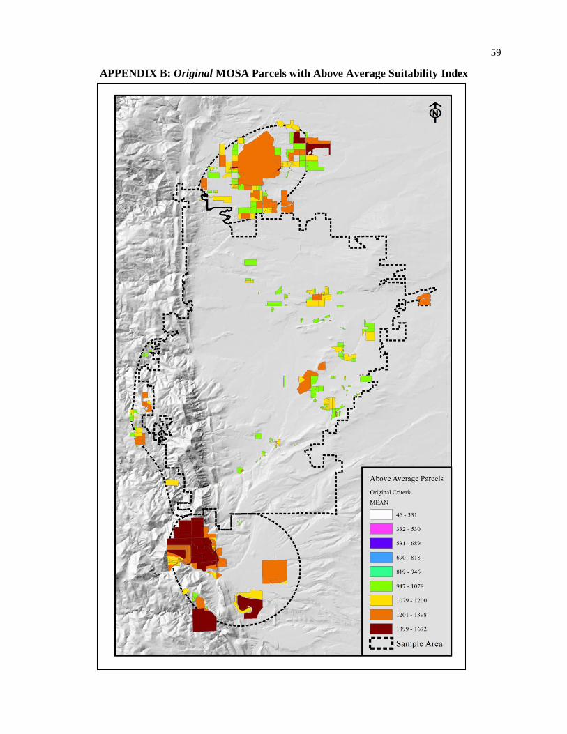
59

APPENDIX B: Original MOSA Parcels with Above Average Suitability Index

60

APPENDIX C: Adjusted MOSA Parcels with Above Average Suitability Index