MODELING OF WAX DEPOSITION IN A CRUDE OIL CARRYING...

!

!!

MODELING OF WAX DEPOSITION IN A CRUDE OIL CARRYING PIPELINE

by

Preston Montalvo

A thesis submitted to the faculty of The University of Utah

in partial fulfillment of the requirements for the degree of

Master of Science

Department of Chemical Engineering

The University of Utah

May 2012

!

!

Copyright © Preston Montalvo 2012

All Rights Reserved

!

T h e U n i v e r s i t y o f U t a h G r a d u a t e S c h o o l

STATEMENT OF THESIS APPROVAL

The thesis of

has been approved by the following supervisory committee members:

, Chair Date Approved

, Member

Date Approved

, Member

Date Approved

and by , Chair of

the Department of

and by Charles A. Wight, Dean of The Graduate School.

Preston Montalvo

Milind Deo 3/21/2012

Jaye Magda 3/21/2012

Rich Roehner 3/21/2012

JoAnn Lighty

Chemical Engineering

!

!

!

!!

!!

ABSTRACT

The oil modeled in this thesis has a large amount of paraffin and must be

transported from where it is extracted to a refinery over a distance that includes changes

in elevation and temperature. This study investigated the deposition that would occur due

to the paraffin in the oil. In this study the paraffin containing oil was mixed with a

diluent in order to lower the wax appearance temperature (WAT) of the oil for one case.

The second case involved mixing the paraffin containing oil with a light crude oil that did

not contain a large amount of paraffins. The cases were modeled using the DepoWax

module found in the commercially available software PVTsim, by Calsep International

Consultants. Both of the cases were modeled in a pipeline, when the weather would be

the coldest due to the ambient temperature being much lower than the WAT. The large

temperature gradient in the pipeline to the outside air causes the temperature of the oil to

drop below the WAT and pipeline pressure to be quite high. High Temperature Gas

Chromatography (HTGC), viscosity measurements and Fourier Transform Infrared

Spectroscopy (FTIR) were used to characterize the oil. The HTGC gave the carbon

number distribution of the paraffin containing oil as well as the diluent. Viscosity

measurements gave rheological values for the oil at different temperatures as well as

different dilutions with the diluent. The FTIR was used to determine the wax appearance

temperature (WAT). The measured values from the previous tests all were used as inputs

to DepoWax to characterize the oil and the mixtures to be modeled in the pipeline.

!

!

CONTENTS ABSTRACT ...................................................................................................................... iii

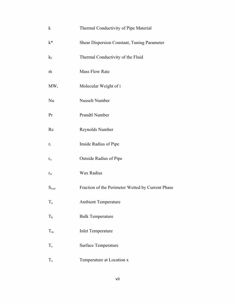
NOMENCLATURE ......................................................................................................... vi

ACKNOWLEDGEMENTS ............................................................................................. x

INTRODUCTION ............................................................................................................ 1

LITERATURE REVIEW OF WAX DEPOSITION ..................................................... 4

2.1 Introduction ................................................................................................................... 4 2.2 Jessen and Howell (1958) ............................................................................................. 4 2.3 Hunt (1962) ................................................................................................................... 6 2.4 Burger et al. (1981) ....................................................................................................... 8 2.5 Weingarten et al. (1986) ............................................................................................... 9 2.6 Brown et al. (1993) ..................................................................................................... 10 2.7 Hsu et al. (1994) .......................................................................................................... 12 2.8 Hamouda et al. (1995) ................................................................................................ 13 2.9 Creek et al. (1999) ...................................................................................................... 14 2.10 Leiroz and Azevedo (2005) ...................................................................................... 16 2.11 Wax deposition as a whole ....................................................................................... 19 2.11.1 Molecular diffusion of wax ............................................................................ 19 2.11.2 Shear dispersion of precipitated wax ............................................................. 20 2.11.3 Brownian diffusion of precipitated wax ........................................................ 20 2.11.4 Gravity settling of precipitated wax ............................................................... 21 2.11.5 Sloughing of wax ........................................................................................... 21

ANALYTICAL MEASUREMENTS FOR THE MODEL ......................................... 22

3.1 Mixing the black wax crude oil and diluent ............................................................... 22 3.2 FTIR analysis .............................................................................................................. 23 3.3 Rheology ..................................................................................................................... 23 3.4 Composition characterization ..................................................................................... 24

RESULTS OF ANALYTICAL MEASUREMENTS ................................................... 25

4.1 FTIR analysis .............................................................................................................. 25 4.1.1 Wax appearance temperature (WAT) .............................................................. 25

!

v!!!

4.1.2 Estimation of solids ......................................................................................... 27 4.2 Rheology ..................................................................................................................... 29 4.3 High temperature gas chromatography (HTGC) ........................................................ 39

MODELING .................................................................................................................... 41

5.1 Introduction to modeling ............................................................................................ 41 5.2 Flow model ................................................................................................................. 41 5.3 Temperature model for the pipeline ............................................................................ 42 5.3.1 Overall heat transfer coefficient ....................................................................... 43 5.3.2 Inner heat transfer coefficient .......................................................................... 43 5.3.3 Outside heat transfer coefficient ...................................................................... 44 5.4 Methods used by DepoWax to predict wax deposition .............................................. 45 5.4.1 Deposition by molecular diffusion ................................................................... 45 5.4.2 Deposition of by shear dispersion .................................................................... 46 5.5 Input of experimental data into PVTsim and DepoWax ............................................. 46

RESULTS OF MODELING AND CONCLUSIONS .................................................. 48

6.1 Description of the model ............................................................................................. 48 6.2 Case one waxy oil and diluent mixture ....................................................................... 48 6.3 Discussion of waxy oil and diluent mixture ............................................................... 54 6.4 Case two waxy oil and light crude mixture ................................................................ 54 6.5 Discussion of light crude and waxy oil mixture ......................................................... 59 6.6 Conclusions ................................................................................................................. 59

APPENDIX: FLASH OUTPUT FROM PVTSIM ...................................................... 61

REFERENCES ................................................................................................................ 66 !

!!!!!!!!

!

vi!!

!!!!!

NOMENCLATURE !

Symbol Definition

A Area Available for Wax Deposition

Cib Concentration of i in the Bulk

Ciw Concentration of i at the Wall

Cp Specific Heat

Cwall Volume Fraction of Wax Deposited at the Wall

d Inner Diameter of the Pipe

Di Diffusion Coefficient of I

Dil Percent of Diluent Added

f Friction Factor

g Gravitational Constant

Gr Grashof Number

hi Inside Heat Transfer Coefficient

ho Outside Heat Transfer Coefficient

!

vii!!

k Thermal Conductivity of Pipe Material

k* Shear Dispersion Constant, Tuning Parameter

kf Thermal Conductivity of the Fluid

ṁ Mass Flow Rate

MWi Molecular Weight of i

Nu Nusselt Number

Pr Prandtl Number

Re Reynolds Number

ri Inside Radius of Pipe

ro Outside Radius of Pipe

rw Wax Radius

Swet Fraction of the Perimeter Wetted by Current Phase

Ta Ambient Temperature

Tb Bulk Temperature

Tin Inlet Temperature

Ts Surface Temperature

Tx Temperature at Location x

!

viii!!

U Overall Heat Transfer Coefficient

v Linear Velocity

VDiff Volumetric Diffusion of Wax

VShear Volumetric Shear Dispersion of Wax

x Location on Pipe

xw Deposit Thickness

Greek

α Thickness Correction Factor, Tuning Parameter

β Diffusion Tuning Parameter

βv Volumetric Thermal Expansion Coefficient

γ Shear Rate

δ Thickness of Laminar Sub-Layer

∂P/∂L Pressure Drop

ε Roughness of Pipe

θ Angle From the Horizontal

µ Viscosity of the Fluid

µb Viscosity of the Fluid in the Bulk

!

ix!!

µw Viscosity of the Fluid at the Wall

ν Kinematic Viscosity

ρ Density

ρi Density of Wax Forming Component i

ρwax Average Density of Wax in the Bulk

!

!!

ACKNOWLEDGEMENTS !! I would like to thank Dr. Milind Deo for his guidance and financial support over

the past year while working on this project. Also working with members of Petroleum

Research Center has been a great learning experience. I would also like to thank Dr. Rich

Roehner for his tutorial on PVTsim, as well as Dr. Magda for his suggestions and also for

serving on my supervisory committee.

My family is also due thanks for their support while working on this project. Also

all of the other graduate students I met throughout my studies at the University of Utah.

!

!

CHAPTER 1

INTRODUCTION

The need for energy is becoming more crucial these days and is causing more

companies to drill for oil that has high paraffin concentrations. The paraffin, also

referred to as wax, poses a large problem when it forms and deposits in pipelines carrying

this oil. The problem is observed in which the ambient temperature is lower than the wax

appearance temperature (WAT), the oil cools and wax will form resulting in deposition.

The deposition of the wax decreases the amount of oil traveling through the pipeline and

also increases pumping costs. This arises from a decrease in diameter for oil flow. Pipe

friction also increases due to solids, i.e., asphaltenes, which can deposit into the wax

formation.

There are methods to deal with wax deposition in pipelines. One method is to

routinely scrape the deposits from the pipe walls. This method is known as ‘pigging’.

Other methods include adding chemicals to inhibit the formation of wax in the pipeline.

There is also introducing hot oil into the system. This will cause the deposit to be

dissolved because it gets heated above its WAT. The problem with this method is that

once the deposit has been dissolved back into the hot flowing oil the oil will cool back

down further down the pipeline and deposition will continue. Mixing a waxy crude oil

with another that does not have as high a wax content is also another method to pump the

waxy oil to its final destination.

!!

2 !

!!

The method employed to deal with wax deposition is based on the cost of the

solution. Regular pigging will keep the pipeline clean and free of deposition. Chemical

inhibitors are quite expensive and they have not been shown to completely eliminate wax

deposition in pipelines. With the use of the chemical inhibitors, eventually the line must

be pigged out adding even more to the cost, although pigging intervals could be at larger

time spans. Also with the blending of two oils together, eventually the pipeline will need

to be pigged using this type of wax management.

The goal of the treatments is to determine how much and how fast the wax

deposit will build up. Using a model to predict deposition thickness over a period of time

as well as operating conditions of the pipeline can lead to a better maintenance schedule.

Many groups have researched the wax phenomenon deposition. However due to

different testing methods and assumptions made there is a discrepancy on exactly how

the mechanisms of deposition occur. There is agreement that the primary mechanisms

are diffusion and shear dispersion of wax. The diffusion of wax can occur by dissolved

wax diffusing to the wall and depositing and also by the diffusion of wax particles, which

have formed in the bulk, to the wall and depositing. Shear dispersion results in transport

to the pipe wall based on shear by precipitated wax particles. Shearing can also affect the

strength of deposit. If the flowing oil exerts a high enough shear on the deposit, it can be

pulled from the wall; this is known as sloughing. When some of the wax sloughs off, the

remaining wax is harder.

This thesis models pipeline flow of a high paraffin containing crude oil. This oil

flows in a pipeline over a distance of approximately 110 miles with large elevation

!!

3 !

!!

changes. The model looks at the addition of a light fraction petroleum distillate, referred

to as a diluent, and also looks at blending the black wax crude oil with a lighter crude oil.

!!

4 !

!!

CHAPTER 2

LITERATURE REVIEW OF WAX DEPOSITION

2.1 Introduction !

Wax can be defined as paraffin deposits that are insoluble in crude oil at the

prevailing producing conditions of temperature and pressure [12]. Wax deposition has

always posed a production problem in the petroleum industry. The topic has been studied

for many years by many different groups of researchers. The aim of the literature review

performed in this chapter is to summarize findings on wax deposition that are available in

the literature.

Each paper in this chapter is analyzed paying attention to the hypothesis, the

methodology employed, observations and the conclusions made.

2.2 Jessen and Howell (1958) Plastic coated pipes used on oil fields, to prevent corrosion, were observed to

have little or no wax deposition. Jessen and Howell [12] wanted to verify if different

types of pipe as well as different flow rates reduced or eliminated deposition.

The apparatus constructed to test their hypothesis consisted of a flow loop with

two test-sections each a length of 5’ but varying diameters of 3/4” and 2”, made either of

plastic, steel or coated pipe with steel being the control. Each pipe material used had the

two test-sections. Cooling was achieved by submerging the test-sections in a water bath

!!

5 !

!!

by circulating water through coils packed in ice. A hot water bath was also used to keep

the circulating oil above its cloud point in the reservoir. Two centrifugal pumps were

used in order to produce turbulent flow. The oil transported through the flow loop

consisted of microcrystalline waxes in kerosene. In order to control the flow rate of the

liquid in the flow loop a series of bypasses were used, this also was used to mix the oil in

the reservoir. The flow rate was measured by using a differential manometer placed on

each of the test-sections. Tests were run for a time period of about 3 hours. Once a test

was completed the test-sections were removed and a tight fitting rubber squeegee was

pushed down the pipe in order to collect the paraffin deposit. The paraffin deposit was

mixed with pentane and centrifuged at 1,500 rpm for 20 minutes; the solids insoluble in

pentane were recorded as paraffin.

Some of the observations made were that the plastic and the coated pipes showed

lower deposition than the steel pipe. Another observation made was that as the flow rate

was increased the amount of paraffin deposition also increased. The deposition reached a

maximum when the flow transitioned from laminar to turbulent flow. Once the flow

transitioned to the turbulent regime the deposition decreased rapidly; the plastic pipes

with Reynolds numbers greater than 4,000 showed no deposition. The researchers

proposed two mechanisms for the paraffin deposition both being due to mass transfer.

They also observed viscous drag of the particles exceeding the shear stresses of the

deposited paraffin, at higher flow rates.

The first mass transfer mechanism is the diffusion of the paraffin to the wall

where the deposit will grow. The second was that paraffin crystals have already formed

in the flowing system in which particle diffusion to the wall occurs. The deposition in

!!

6 !

!!

the plastic pipes was noticed to be 3 times greater at low velocities when the temperature

was 1° F higher than the cloud point than when it was when the oil was 15° F below the

cloud point. In the steel pipe not much of a difference was noticed. At the lower

temperatures the paraffin crystals would increase, but the deposition did not increase.

Since the deposition did not increase with decreased temperature the diffusion of paraffin

to the walls was proposed to be controlling.

The viscous drag, at higher flow rates, was proposed to actually remove some of

the paraffin from the wall, resulting in the decrease of paraffin deposition. The paraffin

deposits at the higher flow rates were also noted to be harder than the paraffin deposits at

the lower flow rates.

2.3 Hunt (1962)

! Laboratory tests, performed by Elton B. Hunt Jr. [10], were completed in order to

determine mechanism of paraffin deposition under similar conditions of well tubing in

the field. The studies were completed under steady flow conditions. The author noted

that cooling was the controlling factor for wax deposition; this conclusion was made due

to no deposition of wax occurring under constant temperature conditions.

The experimental setup consisted of a cold spot apparatus as well as paraffin

deposition apparatus. The cold spot test consisted of a cold finger with a plate that was

soldered on the end of it and submerged in a stirred heated wax-oil slurry contained in a

beaker heated by circulating hot water, while the finger was cooled by circulating cool

water. The slurry temperature was decreased at a constant rate of 1.2° F/hour for 15.5

hours. Upon completion of the experiment the plates were removed and examined for the

amount of deposit, hardness of deposit and the adherence of deposit to the plate.

!!

7 !

!!

A flow loop, for deposition studies, was constructed to mimic the gradients under

field conditions. Oil was pumped, at a constant rate from a reservoir maintained at 200°

F, through a vertical test section up of 23.3’, 1/8” pipe. A precooler was used to cool the

incoming oil to the desired temperature at the inlet of the test section. A separate

recirculation pump mixed the test section fluid. To prevent oxidation of the hot oil a

nitrogen blanket and an oxidation inhibitor were used. The flow loop had two different

versions consisting of a high and low temperature gradient used. The experiments were

run for 21.5 hours to 155 hours. Once a test was completed the test section was drained

and dismantled in some cases the test section was cut into 10” lengths. The dismantled

test section was then visually examined and weighed to determine the amount of deposit.

The oil was evaporated off of the deposit and then weighed to determine the amount of

wax deposited. It was noted that no wax was lost during evaporation.

It was observed that inside the test section specks of wax appeared at the pipe

wall near the inlet and become a continuous film of increasing thickness towards the top

of the test section. As time increased the deposit became a continuous film throughout

the test section. From the results of the visual observations it was proposed that

deposition was initiated by direct nucleation of wax on or adjacent to the pipe wall and

that the deposit grows by the diffusion of wax to the previously deposited wax. Both the

low and high temperature gradient tests gave similar results. From the results of the low

and high temperature tests it was concluded that the deposition mechanism does not

change when decreasing the temperature gradient.

The results of the cold spot test showed that the wax did not adhere to smooth

stainless steel but did adhere to sand blasted stainless steel. It was also observed that the

!!

8 !

!!

wax did not adhere to smooth plastic coatings but did adhere when the plastic was

roughened by sandpaper. Similar results were made in the test sections. This led to the

conclusion that the wax does not adhere to the surface but is held in place by the

roughness and/or irregularities of the surface.

2.4 Burger et al. (1981)

! Wax deposition was occurring at the southern end of the Trans Alaskan Pipeline

(TAPS), even though the flow rate was high, 1.5 million barrels per day. Burger, Perkins

and Striegler [4] wanted to investigate the mechanisms of wax deposition and also

wanted to determine the expected nature and the thickness of the deposits found in TAPS.

To study the deposition an experimental set up was constructed. The setup consisted of

2.9 m long, 6.35 mm and 12.7 mm stainless steel tubes in parallel horizontal and also

parallel vertical configurations. Each of the tubes had its own oil and coolant pumps,

allowing independent operation of each tube. All of the tubes were operated under totally

laminar conditions and were scaled with wall shear stress rather than the Reynolds

number. The temperature and heat flux values were kept in the range of TAPS during

initial start-up and early flow. Flow tests lasted from 2 to 200 h, in which the oil and the

coolant were both pumped at constant rates. At the end of each test, once the oil was

removed, the tubes were heated to 50° C and washed with toluene, for the small diameter

tubes. The large diameter tubes were cleaned with a scraper. The amount of deposited

wax was determined by the acetone precipitation technique mentioned in the paper.

Field test experiments were also completed on 2440 m long with diameters of 10, 15 and

20 cm. Six test sites were spaced at 490 m along each of the pipelines. Each test site had

!!

9 !

!!

60 cm spool pieces that were removed, at various time intervals during a test, and the wax

scraped to determine the weight and the crystal content.

The total deposition was modeled as the sum of three lateral transport

mechanisms molecular diffusion of wax, Brownian diffusion and shear dispersion of the

wax particles. Gravity settling was studied for both the horizontal and vertically

arranged tubes, but showed no significant effect. The researchers mention that shear

dispersion might redisperse settled solids, eliminating any gravity settling effect.

The authors concluded that deposition occurs due to the transport of dissolved and

precipitated wax crystals under the conditions in which the oil is cooling. Under different

conditions the rate-controlling step varies upon conditions being tested. At high

temperature and high heat flux conditions molecular diffusion is controlling, while under

the conditions of TAPS, lower temperatures and low heat fluxes, shear dispersion is

controlling. It was also found that Brownian diffusion is small when compared to the

other mechanisms.

2.5 Weingarten et al. (1986)

! Burger [4] described the methods of primary wax deposition to be molecular

diffusion, mass diffusion, and shear dispersion. Weingarten and Euchner [21]

investigated the two mechanisms independently of one another.

In order to measure deposition due to diffusion only a diffusion cell was built. In

the cell the oil was kept static while one end of the cell was heated and the other cooled,

to create a temperature gradient. The tests lasted for 48 h to 170 h, with each end

maintained at constant temperature. At the end of each test the oil was drained, the cell

disassembled and the deposit weighed. The amount of wax was determined by using the

!!

10 !

!!

same acetone precipitation technique used by Burger [4]. The results of the diffusion

tests found the wax fraction to be constant at 0.18.

The shear dispersion mechanism was also investigated. A flow loop consisting of

1/4” stainless steel tube, for oil, inside a 1/2” copper tube, used to control temperature.

Pressure drop across the test section was continuously monitored to calculate the volume

of the deposit, assuming the deposit is uniform. The temperature of the oil ranged from

37° F to 66° F, heat transfer rates of 6 BTU/h-ft2 to 1840 BTU/h-ft2 and shear rates from

12 s-1 to 4960 s-1 were used. Oil temperatures below the wax crystallization temperature

were preferred so that the deposition due to diffusion could be accurately measured.

Low and high shear rate tests were performed. The rate of deposition due to diffusion

and shear dispersion were plotted on the same graph in order to compare results. The low

shear rate experiments showed the deposition to gradually increase over time. The

deposition over time was greater than that only due to diffusion, which confirmed shear

dispersion as a mechanism. The high shear rate tests showed a rapid increase in

deposition, similar to diffusion, followed by a decrease and finally resulting in a rate of

zero deposition. The decrease of wax deposition was attributed to sloughing off of the

wax deposit. The flow for the high shear test remained laminar throughout, meaning that

the sloughing occurred when the wall shear stress was greater than that of the wax

deposit, not due to turbulence.

2.6 Brown et al. (1993)

! Deposition of wax under flowing conditions was studied by Brown, Niesen and

Erickson [3]. The results of the experimental tests were then put into a computer model

to predict deposition rates at the long term.

!!

11 !

!!

The experimental setup consisted of 1/4” and 3/8” stainless steel tubing, each 39”

long, submerged in a water bath to control the temperature. Continuous measurements of

inlet, outlet and wall temperature were recorded, as well as the pressure drop and the flow

rate across the test section. Under laminar flow conditions the deposition thickness can

be calculated based on the flow rate and pressure drop, assuming a uniform deposit. The

calculated deposition was also compared to the actual deposition by collecting the

paraffin and weighing it.

Using Burger’s [4] equations of molecular diffusion and shear dispersion, the

shear dispersion was tested. To test the shear dispersion mechanism tests were completed

at varying shear rates, while maintaining a constant inlet and wall temperature, not a zero

flux. At the increased shear rate the deposition actually decreased rather than increased

linearly as suggested by Burger. A zero heat flux case was also tested because no

molecular diffusion would occur, and shear deposition would be unaffected. No

deposition occurred under the zero heat flux condition so it was concluded that shear

dispersion does not contribute to deposition.

The modeling of the deposition allows for varying the diffusion coefficient in

order to fit experimental data; essentially it has become a data fitting parameter. The

model also assumes that the rate of paraffin deposition is slow compared to the rate at

which the pipeline comes to a new steady state. It is mentioned that although the

pressure drop is a primary variable in the model the roughness of the deposit is much

more important, but in the model the roughness value is the same as the thickness of the

deposit.

!!

12 !

!!

2.7 Hsu et al. (1994) ! Most studies involving wax deposition consist of circulating the wax containing

crude oil under laminar conditions. Hsu, Santamaria, and Brubaker [11] studied

deposition under turbulent conditions.

To conduct the deposition studies a flow loop was built. The flow loop consisted

of two identical test sections. The test sections were each 5’ long and 0.402” inner

diameter stainless steel. The first referred to as the ‘test tube unit’ was used to test for

deposition at various operating conditions. The ‘reference tube’ was maintained above

the oil temperature to inhibit deposition and also used to measure pressure drop to

compare to the ‘test tube unit’ in order to calculate the deposition thickness. Temperature

was controlled on each test section using a cooling jacket. The volumetric flow rate,

fluid density, system pressure, pressure across the test sections and temperature at various

locations were all recorded. At the end of the test nitrogen was used to purge the test

sections and then the lines were pigged.

Under turbulent conditions it was found that wax deposition decreased. It was

also found that turbulent conditions depress the temperature at which the maximum

deposition rate occurs, meaning that the actual pipeline could be operated at lower

temperature. The decrease in deposition was explained by a sloughing effect. The higher

flow rate created higher shear stresses removing some of the deposit from the wall.

At the completion of each test the tubes were pigged out and the deposit analyzed

by simulated distillation and melting point. It was found that with an increase in

retention time the deposit showed increases in both hardness and carbon number. At

lower oil temperatures the deposit formed was found to be softer. When the oil

!!

13 !

!!

temperature approached the ambient temperature, i.e., low heat flux, the deposit was

softer and more homogeneous.

2.8 Hamouda et al. (1995)

! Of all the deposition mechanisms Hamouda and Davidsen [8] wanted to show that

deposition by molecular diffusion is dominant.

The experimental setup consisted of a series of heat exchangers, where oil was

kept heated in a tank to maintain temperature while being pumped. The primary heat

exchanger, which was the test section, was 25 m long and 1/2" diameter pipe made of

aluminum inside of 1” diameter stainless steel pipe. Temperature and pressure

measurements were made in every loop of the heat exchanger. Deposition was calculated

by measuring the pressure drop across predetermined lengths of pipe. Flow rates were

also varied 5 to 11 L/min. The oil was also put under a nitrogen blanket to minimize

oxidation.

To study the deposition mechanisms the test pipe was divided into three sections

15, 5 and 5 m. In the first section, 15 m, the oil was cooled from 27° C to 18° C. In the

second section, 5 m, the temperature was kept at 17° C. This was done to minimize the

temperature gradient to eliminate molecular diffusion. In the final section, 5 m, the

conditions of the first section were restored.

The deposition increased between 5 and 7.7 L/min, with a maximum deposition

rate at 7.05 L/min. The increase in deposition at these flow rates were due to molecular

diffusion and/or shear dispersion, where the temperature and concentration gradient are

both factors. Above 7.7 L/min the deposition drastically decreased and zero deposition

!!

14 !

!!

occurred at 11 L/min. Deposition decreased due to the increase in the shear stress, which

results in the removal of deposition from the wall.

In the second section almost no deposition occurred. If an appreciable amount of

deposition occurred shear dispersion would have been considered a larger contributing

factor. It was concluded that the shear dispersion is small compared to molecular

diffusion and is not a major mechanism.

The investigators also found that deposition occurred for shear rates between

3500 s-1 and 5500 s-1, above the maximum shear rate no deposition was detected. To

determine the amount of the deposit a ‘paraffin adhesion constant’ was defined. This was

multiplied by the sum of the amounts of deposition due to shear dispersion and molecular

diffusion. When the shear rate was above 5500 s-1 the constant was set to 0 and when the

shear rate was below 3500 s-1 the constant was set equal to 1. The higher shear rate

coincides with the higher flow rate at which no deposition was detected.

2.9 Creek et al. (1999)

! Experiments to determine the effects of flow rate and temperature difference on

deposition rate, as well as the fraction of oil in the deposit, were performed for single-

phase flow by Creek et al. [6]. In this case the shear dispersion was considered

insignificant based on previous findings [8].

The flow loop was 50 m long, 43.4 mm inner diameter configured as a horizontal

‘U’. The entire tube was jacketed to control temperature. At every 5 m along the tube

temperature and pressure measurements were taken. Wax deposits were collected from

removable spools located at 20 m from the inlet and 5 m from the outlet. Flow rate of the

oil and coolant was also measured. Pressure drop, energy balance based on temperature

!!

15 !

!!

difference, volume changes in the test section, ultrasonic transit time and direct

measurement were the different methods used to determine deposit thickness in the study.

The fraction of oil in the deposit was determined by high temperature gas

chromatography. Modeling software, from Multiphase Solutions Inc. by Brown [3], was

also used alongside the experiments.

The temperature difference between the oil and wall was the first study

performed. Both laminar and turbulent flow was tested for this case. Both show a linear

increase in deposition with the laminar case having thicker deposits. The deposits found

in the test section under the laminar case were found to be much softer than for the

turbulent case. Another note about deposit hardness was that the larger the difference in

temperature between the oil and the wall, the softer the deposit. The modeling software

followed the same trend as the experimental results and gave near what was measured for

deposition [3].

Another test that was performed was to keep a constant temperature difference

between the pipe wall and flowing oil of 8.3° C while decreasing the inlet temperature of

the oil to as much as 25° C below the wax appearance temperature (WAT). These tests

were performed under laminar conditions. It was also found that no deposition was

observed when there was no temperature difference. The modeling software for this case

also gave the same trend but there was more scatter among all the methods used to

calculate deposit thickness [3].

Using the same temperature difference of 8.3° C between the flowing oil and the

wall, the effect of varying flow rate was also tested. As the flow rate was increased it

was found that the deposit thickness decreased. This was true for both turbulent and

!!

16 !

!!

laminar flow. The result from the turbulent tests showed that the wax content of the solid

was between 60 and 80%. Sloughing was also mentioned as the reason why the deposit

decreased in thickness over time. The modeling software showed the inverse of what

was measured for increasing flow rate. It showed an increase in deposit thickness and

then a decrease [3].

During the measurements of the deposition thickness the energy balance method

was found to fit the data for deposition thickness more accurately for laminar flow

conditions. The pressure drop method for calculating deposit thickness proved to be

more accurate for turbulent flow conditions.

2.10 Leiroz and Azevedo (2005)

Leiroz and Azevedo [13] noticed that in models predicting wax deposition

constants were adjusted in order to fit the predictions of the model for the actual data

collected, either from the field or laboratory. This was good for a specific scenario, but

not the importance of individual mechanisms. The study used experiments and numerical

analysis to study diffusion-based mechanisms.

The study employed two deposition tests, both using a model oil. The first test

for deposition was under stagnant conditions. The model oil for the stagnant tests

consisted of a 10% by volume solution of paraffin. The paraffin solution consisted of

carbon numbers of C21 to C38. The paraffin solution was then dissolved in n-paraffin.

The WAT for the model oil was determined to be 27° C the properties of the oil were

also known. The experimental set up for the stagnant tests consisted of a deposition cell.

The cell had dimensions of 10 x 30 x 0.5 mm. The 0.5 mm was the area available for

deposition this was made by “sandwiching” two pieces of glass together, held in place by

!!

17 !

!!

copper fins. The fins had thermocouples attached to each to record the temperature. The

oil was pumped into the cell, and temperature in the cell was maintained above the WAT.

During the test one side of the cell remained hot and the other side was cooled. This

allowed for the deposition to be recorded and digitized.

The experiments under laminar flow conditions used a model oil with a WAT of

36° C and consisted of a rectangular test section with dimensions of 3 x 10 x 300 mm.

The walls of the test section were made of 2 mm glass plates and the top and bottom of

the test section was made of copper, which was soldered to hollow copper blocks. The

copper blocks had water pumped through them, in order to control and maintain

temperature. Temperature was monitored by thermocouples attached to the copper walls.

The temperature of the oil was controlled upstream with a coil-tube heat exchanger. An

electric heater heated a smaller tank downstream, previous to the test section, in order to

avoid deposition before entering the test section. To study the deposition the oil was

allowed to flow above the WAT until a steady state condition was achieved, after steady

state was achieved cold water was circulated through the copper blocks to cool the test

section. To visualize the whole length of the test section, the flow rate was set and a

camera was set at a specified location once the cooling began the camera began to record

the test section. After deposition was achieved, the copper blocks were heated to remove

the deposition and the test was repeated under the same conditions with the camera

moved further down the test section. This was done until the entire test section was

recorded.

Simulations of the experiments were also completed. The model for the stagnant

experiment consisted of the following assumptions: one-dimensional heat and mass

!!

18 !

!!

transfer, constant properties and saturated liquid at the solid fluid interface. The model

for the laminar flow system assumed one-dimensional flow, with velocity varying in the

axial direction due to the deposition of wax. The flow also employed the use of a friction

factor. Heat losses were also calculated for each of the walls. Burger’s [4] molecular

diffusion model accounted for the growth of the deposited layer.

When the results were modeled for the stagnant condition it was concluded that

the model for molecular diffusion under predict the actual amount of deposition. This led

the authors to believe that the other mechanisms do play a role, although heat losses in

the walls of the deposition cell were not considered.

From the experimental results of the laminar flow condition it was observed that

the deposition on the top of the test section was equal to the deposition on the bottom of

the test section. The symmetry of the deposition visually showed that gravity settling

was not a relevant mechanism of deposition. The authors also found that in their

experiments within the first 10 minutes of testing the deposition was about 50% of the

final steady state deposition. Another observation made by the authors was that with

increase of axial length, deposition increases, while the model predicts a decrease. The

only agreement of data came from the steady state condition, in which both the

experimental results and the model show an increase in deposition. The conclusion of

the study shows that the models under predict the actual deposition when only molecular

diffusion is considered. This implies that other mechanisms do in fact play a role in

deposition.

!

!!

19 !

!!

2.11 Wax deposition as a whole ! In this area many groups have researched and proposed ideas of the mechanisms

of deposition. Many experiments have been carried out to study this phenomenon. The

experiments carried out either were used to focus on one type of deposition mechanism or

to study it as a whole. The purpose for carrying out this research is to predict the amount

of wax deposited as well as the properties of the deposit. This is very important in order

to mitigate wax deposition. It has been found that changing certain operating parameters

can help to minimize the deposition of wax in a pipeline. It is also useful to know, if

deposition cannot be prevented, when treatment of the pipeline may become necessary.

The treatments can include chemical inhibitors or mechanical methods (pigging). From

the literature reviewed previously the mechanisms of deposition were found to be:

1. Molecular diffusion of dissolved wax

2. Shear dispersion of precipitated wax

3. Brownian diffusion of precipitated wax

4. Gravity settling of precipitated wax

5. Sloughing of wax

2.11.1 Molecular diffusion of wax !

Molecular diffusion of wax is based on a concentration difference. It is also

affected by temperature gradients within the flowing pipeline. This problem can be seen

in pipelines in which the oil is flowing below the Wax Appearance Temperature (WAT)

over long distances. With oil being a mixture of many different hydrocarbons

concentration gradients will develop rapidly once the oil temperature falls below the

WAT, due to each component having its own temperature dependence on solubility in the

!!

20 !

!!

solution. This mechanism of deposition has been found to be very important in

deposition studies and has also been confirmed by many different groups [3, 4, 6, 8, 13].

Molecular diffusion of wax will be investigated later in this thesis using the DepoWax

module found in PVTsim by Calsep International Consultants.

2.11.2 Shear dispersion of precipitated wax ! Shear dispersion occurs when the wax particles move across fluid streamlines due

to differences in shear imparted by other flowing particles. The particles in solution

rotate as they flow, and due to the viscosity of the fluid the rotating particles will impart a

shear force on nearby particles. In a high presence of particles the interactions between

them will increase and the lateral transport of wax particles will occur across the

streamlines toward the wall and deposit. Shear dispersion is considered to be one of the

major mechanisms in wax deposition and appears to play a bigger role at lower

temperatures as well as lower heat fluxes [3, 4, 6, 21]. Shear dispersion is the second

mechanism considered in the DepoWax module and will be used in the modeling of wax

deposition in this thesis.

2.11.3 Brownian diffusion of precipitated wax ! Brownian diffusion of precipitated wax is based on random movements of the

precipitated particles. This is also affected by concentration of wax particles in solution.

Typically the particles in solution will have no net displacement. In the case of high

concentration of suspended wax particles in a flowing system, collisions will increase and

the particles will move towards the wall where there is a lower concentration. Brownian

diffusion is not considered to play a pivotal role in wax deposition because it is small

!!

21 !

!!

compared to other mechanisms of wax deposition. As mentioned by Burger [4],

Brownian diffusion was prominently mentioned in the USSR literature. In this thesis

Brownian diffusion is not considered.

2.11.4 Gravity settling of precipitated wax ! Gravity settling occurs when a heavier particle settles due to the force of the

Earth’s gravity. Wax particles are denser than the surrounding fluid and will begin to

settle out under stagnant conditions. Under flowing conditions, especially under

turbulent conditions, as the particles settle out the flow can cause settled wax particles to

return to the bulk. The shear dispersion can also remove the wax particles that have

settled out due to gravity. Due to the previously mentioned reasons, gravity settling of

wax particles is not considered to play a large role in wax deposition.

2.11.5 Sloughing of wax ! In sloughing of wax the wax layer actually decreases in thickness [3, 8, 11, 12].

This arises from the shear stress felt by the deposit on the wall. When the shear stress

increases beyond the yield stress of the deposit, the deposit is sloughed off. This

mechanism is not studied in this thesis but does play a vital role for the restart of plugged

pipelines.

!!

22 !

!!

CHAPTER 3

ANALYTICAL MEASUREMENTS FOR THE MODEL

The DepoWax module in PVTsim allows the fluids to be characterized based on

analytical measurements. The use of the analytical measurements in the modeling

software allows for a more accurate simulation.

The analytical measurements were performed on the black wax crude oil, as well

as other samples of the black wax crude oil with a diluent added at varying weight

percentages. The measurements that were performed were wax appearance temperature

and estimation of solids percentage, viscosity and compositional characterization.

3.1 Mixing the black wax crude oil and diluent

!The crude oil the oil had to be heated, since it was solid at room temperature. The

crude oil was heated in a beaker on a hot plate with a stirrer inside until it melted and

became possible to transfer a known amount. The diluent was liquid at room

temperature, made up of mostly light end carbons. The mixing was done based on

weight percent. First the crude oil, once melted, then it was transferred to sample bottle

using a Pasteur pipette that was placed on a digital scale that was zeroed. The amount of

oil and diluent mixed in the sample bottle all depended on the weight percent of the

mixture being tested. The samples prepared were a 10%, 30% and 50% by weight

!!

23 !

!!

diluent mixture. Once these were mixed the sample bottles were capped, to eliminate

evaporation of diluent, and labeled in order to perform analytical tests on them later.

3.2 FTIR analysis

!WAT and an estimate of the amount of solid wax in the sample at different

temperatures were determined using an FTIR technique developed by Roehner [18].

Using this method, the IR spectra of the crude oil (4000 cm-1 to 600 cm-1) were

obtained for temperature ranges varying from sample to sample. The temperature ranged

from 60 °C to 3.0 °C. IR absorbance of the sample was measured in a temperature

controlled liquid cell that was held between clear and polished NaCl windows in a Perkin

Elmer FTIR Spectrometer. Sixteen scans were performed at each of the temperatures

used.

The area of interest of the samples was the peak area found between the range

735-715 cm-1, attributed to the rocking vibrations of long chain methylene groups. The

software included with the spectrometer calculated the peak area. A plot of the peak area

versus temperature was created in a spreadsheet where the WAT was determined and the

solids weight percentage was estimated.

3.3 Rheology

! Below the WAT the crude oil displays time-dependent, non-Newtonian shear

thinning behavior, as the shear stress increases the viscosity of the fluid decreases. The

viscosity measurements were performed on the black wax crude oil as well as the 10%,

30% and 50% by weight diluent mixtures.

!!

24 !

!!

Viscosity was measured using a Brookfield DV-II+ cone and plate viscometer. A

sample size of 1.0 mL was used for each of the viscosities measured. Once the sample

was placed, the plate was locked in place creating a closed system for the sample. Once

locked in place the plate was then heated above the WAT to remove any memory from

the sample. Viscosities were measured at varying temperatures by setting a

predetermined temperature and allowing the sample to come to equilibrium at that

temperature. Using different shear rates, at the maintained temperature, viscosity was

measured to get a time-independent value of viscosity. The viscosity collected was a

function of temperature as well as shear rate.

3.4 Composition characterization

! To obtain a carbon number distribution of the black wax crude oil, high-

temperature gas chromatography (HTGC) was performed on it as well as the diluent.

The carbon number distribution plays an important role when characterizing the fluids in

the DepoWax module.

The procedure used for this was an HTGC simulated distillation (HTGC-SimD)

[7] based on ASTM D-5307 [19]. This procedure results in the total weight percent of

the single carbon number (SCN), along with the weight percentages of n-alkane and non-

n-alkanes of each SCN. The modified procedure gives the weight percentages of SCNs

up to SCN 80. The n-alkane corresponds to the paraffin content, to get wax fraction the

n-alkane weigh percent is divided by the SCN. These tests were completed at the Energy

and Geoscience Institute at the University of Utah.

!!

25 !

!!

CHAPTER 4

RESULTS OF ANALYTICAL MEASUREMENTS

The results from the analytical measurements performed, as described in the

previous chapter, are presented here. The results from the analytical measurements play

a large role in characterizing the fluids in the DepoWax database. Use of the analytical

measurements allows for the model to more accurately represent the flow in the pipeline.

4.1 FTIR analysis

4.1.1 Wax appearance temperature (WAT)

FTIR analysis was performed on the black wax crude oil and the 10%, 30% and

50% by weight diluent and crude oil mixtures. The WAT decreased with increasing

amounts of diluent. The WAT showed a linear trend for the case of no addition of

diluents to adding 50% diluent by weight and is given by the following equation:

WAT = −38.98 ∗ D+ 41.27 (4.1)

where D represents the percent of diluent added. Values of WAT for each of the

different amounts of diluent are shown in Table 4.1. Also shown in Figure 4.1 is the

linear trend that the WAT followed for different dilutions tested.

!!

26 !

!!

Table 4.1 WAT from FTIR analysis. Weight %

Diluent Wax Appearance Temperature (°C)

0 41 10 37 30 31 50 21

Figure 4.1 WAT for different amounts of diluent added.

20

25

30

35

40

45

0% 10% 20% 30% 40% 50%

Wax

App

eara

nce

Tem

pera

ture

(°C

)

Wt% Diluent

!!

27 !

!!

4.1.2 Estimation of solids !

Also with the WAT an estimation of solids percentage was completed on the

same samples. Each of the samples shows a similar behavior that was expected as the

temperature continues to decrease the amount of solids increase. Eventually the solids

amount levels off showing that all of the solids have precipitated out of solution. Similar

to the WAT, when the amount of diluent was increased the amount of solids in the

sample decreased. The weight percent solids vs. temperature graphs are shown for each

of the samples in Figure 4.2 to Figure 4.5.

!

Figure 4.2 Weight percent solids for the black wax crude oil.

8.00

10.00

12.00

14.00

16.00

18.00

20.00

0 5 10 15 20 25 30 35 40

Wt%

sol

ids

Temperature (°C)

!!

28 !

!!

Figure 4.3 Weight percent solids for the 10% by weight diluent mixture.


2.00

4.00

6.00

8.00

10.00

12.00

14.00

16.00

0 5 10 15 20 25 30 35

Wt%

Sol

ids

Temperature (°C)

4.00

5.00

6.00

7.00

8.00

9.00

10.00

11.00

0 5 10 15 20 25 30

Wt%

Sol

ids

Temperature (°C)

!!

29 !

!!


4.2 Rheology ! The viscosity of the waxy crude oil increases rapidly as the temperature decreases

and then becomes a solid once it has cooled below its WAT. With the oil turning to a

solid once it continues to cool below its WAT the pipeline the oil is flowing in can

become plugged. With the addition of the diluent to the waxy sample the viscosities were

affectively decreased. With increasing amounts of diluent added viscosities were

decreased from the original black wax. The values of the viscosity and strain rate are

both used in the DepoWax module. Viscosities vs. strain rate at varying temperatures are

shown in Figure 4.6 to Figure 4.9. Accompanying the previously mentioned figures are

Table 4.2 to Table 4.5 showing the strain rate, shear stress and temperature of each of the

samples.!!

!

4.00

4.50

5.00

5.50

6.00

6.50

7.00

7.50

0 2 4 6 8 10 12 14 16 18 20

Wt%

Sol

ids

Temperature (°C)

!!

30 !

!!

Figure 4.6 Viscosity of the waxy crude oil at varying temperatures and shear rates.

20

200

2000

20000

200000

0 50 100 150 200 250

Vis

cosi

ty (c

P)

Shear Rate (s^-1)

35 C

37 C

40 C

43 C

45 C

50 C

60 C

!!

31 !

!!

Figure 4.7 Viscosity of the 10% by weight diluent mixture at varying temperatures and shear rates.

10

100

1000

10000

100000

0 50 100 150 200 250

Vis

cosi

ty (c

P)

Shear Rate (s^-1)

30 C

35 C

40 C

50 C

60 C

!!

32 !

!!


10

100

1000

10000

100000

1000000

0 50 100 150 200 250

Vis

cosi

ty (c

P)

Shear Rate (s^-1)

25 C

27 C

30 C

33 C

35 C

40 C

50 C

60 C

!!

33 !

!!


1

10

100

1000

10000

100000

1000000

0 50 100 150 200 250

Vis

cosi

ty (c

P)

Shear Rate (s^-1)

10 C

15 C

20 C

25 C

30 C

40 C

50 C

!!

34 !

!!

Table 4.2!Shear stress and strain rate at varying temperatures for the waxy crude oil.!Temperature (°C) Shear Stress (Pa) Strain Rate (s^-1)

60 66.8 200 60 33.4 100 50 108.1 200 50 57 200 50 25 40 50 13.8 20 45 161.2 200 45 84.5 100 45 37.4 40 45 19.7 20 45 11.8 10 43 218.2 200 43 116 100 43 51.1 40 43 29.5 20 43 17.7 10 40 753 200 40 469.9 100 40 291 40 40 222.2 20 40 182.8 10 37 1230 100 37 849.3 40 37 743.1 20 37 709.7 10 37 692 5 35 1708 40 35 1537 20 35 1486 10 35 1449 5 35 1421 4 35 1366 2 35 1187 1

!!

35 !

!!

Table 4.3 Shear stress and strain rate at varying temperatures for the 10% by weight diluent mixture.

Temperature (°C) Shear Stress (Pa) Strain Rate (s^-1) 60 31.5 200 60 15.7 100 50 27.5 200 50 13.8 100 40 241.8 200 40 143.5 100 40 76.7 40 40 49.2 20 35 815.9 200 35 536.7 100 35 344.1 40 35 277.2 20 30 1095 10 30 1018 5 30 998 4 30 985 2 30 924 1

!!

36 !

!!

Table 4.4 Shear stress and strain rate at varying temperatures for the 30% by weight diluent mixture.

Temperature (°C) Shear Stress (Pa) Strain Rate (s^-1) 60 27.5 200 60 13.8 100 50 45.2 200 50 22.6 100 40 100.3 200 40 52.1 100 35 450.2 200 35 273.3 100 35 153.3 40 35 118 20 35 80.6 10 33 723.5 200 33 475.8 100 33 308.7 40 33 245.8 20 33 204.5 10 30 1260 100 30 906.3 40 30 792.3 20 30 759 10 30 723.5 5 30 719.6 4 30 613.4 2 30 442.4 1 27 1757 40 27 1549 20 27 1474 10 27 1437 5 27 1427 4 27 1013 2 27 812 1 25 1633 2 25 1303 1

!!

37 !

!!

Table 4. 5 Shear stress and strain rate at varying temperatures for the 50% by weight diluent mixture.

Temperature (°C) Shear Stress (Pa) Strain Rate (s^-1) 50 11.8 200 50 5.9 100 40 17.7 200 40 9.83 100 30 145.5 200 30 88.5 100 30 49.2 40 30 31.5 20 30 21.6 10 25 414.9 200 25 273.3 100 25 180.9 40 25 149.4 20 25 133.7 10 20 713.7 100 20 479.7 40 20 436.5 20 20 420.7 10 15 1299 100 15 1010 40 15 855.2 20 15 841.4 10 15 772.6 5 15 640.9 2 10 1480 10 10 1311 5 10 1280 4 10 1234 2 10 1101 1

!!

38 !

!!

4.3 High temperature gas chromatography (HTGC)

Characterization of the oil by HTGC was also used to characterize the fluid in the

DepoWax module. The waxy crude oil had carbon numbers as high as C81. The

distribution can be seen in Figure 4.10. The diluent used also had the HTGC procedure

performed on it and consisted of carbon numbers below 10; this distribution is shown in

Figure 4.11. The light crude oil used in the modeling process was previously used [14] in

another study. The carbon number data, from the previous study, were used to

characterize the light crude oil and can be seen in Figure 4.12.

Figure 4.10 Carbon number distribution of the waxy crude oil.

0 0.25 0.5

0.75 1

1.25 1.5

1.75 2

2.25 2.5

2.75 3

3.25

10 15 20 25 30 35 40 45 50 55 60 65 70 75 80

Wt%

Carbon Number

!!

39 !

!!

Figure 4.11 Carbon number distribution of the diluent.

Figure 4.12 Carbon number distribution of the light crude oil.

0

5

10

15

20

25

30

35

5 6 7 8 9 10

Wt%

Carbon Number

0

0.5

1

1.5

2

2.5

3

3.5

4

4.5

5

5 10 15 20 25 30 35 40 45 50 55 60

Wt%

Carbon Number

!!

40 !

!!

CHAPTER 5

MODELING

5.1 Introduction to modeling ! The modeling conducted in this thesis was performed using a commercially

available simulation package. The program, PVTsim by Calsep International

Consultants, contains a module called DepoWax. This module makes it possible to

predict wax deposition in crude oil carrying pipelines. As described in the previous

chapters the modeling of the flow becomes more reliable if analytical measurements are

made in the lab and the oil that is being modeled is characterized. Without the

characterization of the oil being used PVTsim can calculate properties of the oil based on

thermodynamic calculations. However these calculations may not be the same as what

was measured in the lab. The following section describes the methods the DepoWax

module employs to model the deposition of wax in the pipeline [16, 17].

5.2 Flow model

! In DepoWax there are two flow models used one for single-phase flow and

another for two-phase flow. Single-phase flow was only considered in this thesis. The

flow model is given by

!"!" !"#$%

= !!" !"# ! + !!!!! (5.1)

!!

41 !

!!

where ! is the density fluid, g is the acceleration due to gravity, ! is the angle of the

pipeline from the horizontal, ! is the linear velocity and d is the inner diameter of the

pipeline. The term f is the friction factor and is a function of the roughness of the pipe, !,

inner diameter and the Reynolds number. The friction factor can be calculated from the

following expression

f = 5.5×10!! 1+ 2×10! !! +!"!!"

! ! (5.2)

The Reynolds number is the ratio of inertial to viscous forces.

Re = ! !!"! (5.3)

5.3 Temperature model for the pipeline

! The rate of heat transfer from the oil through the pipe wall and to the environment

or vice versa depending on the time of year or location of the pipeline is a very important

factor in the transport of the wax containing oil. As the temperature begins to drop the

amount of wax appearing in solution will increase. An energy balance is used in which

the pipeline is divided into sections and a temperature can be calculated at a position x.

T! = !T! + T!" − T! exp !!!"!!!

x (5.4)

From the above equation a temperature profile can be calculated with knowledge of the

mass flow rate ṁ, the specific heat Cp, pipeline diameter d and the overall heat transfer

coefficient U. Ta represents the ambient temperature and Tin is in temperature of the

inlet.

!!

42 !

!!

5.3.1 Overall heat transfer coefficient ! The overall heat transfer coefficient takes into account the inner, hi, and outer heat

transfer, ho, coefficients as well as the thermal conductivity, k, of the pipeline and is

calculated by

U = !!!! !!!!!

+!" !!!!!!

!!!!,!!!!! + !

!!!!

!!

(5.5)

in this equation ri is the inner radius and ro the outer radius. The term ki-1,I represents the

thermal conductivity of the wax between the two radii ri-1 and ri. As the deposition

increases the program uses an additional layer wax radius, rw, which is a function of

deposit wax thickness, xw, and the inner radius of the pipe and is given by

r! = r!" − x! (5.6)

5.3.2 Inner heat transfer coefficient ! The inner heat transfer coefficient depends on the flow regime laminar,

transitional or turbulent and is based on the Nusselt number,

Nu = ! !!!!! (5.7)

where kf represents the thermal conductivity of the fluid. The Nusselt number can be

calculated from correlations to the dimensionless Reynolds and Prandtl numbers,

Pr =! !!!!! (5.8)

The correlations are also based on what flow regime the fluid is in. DepoWax uses the

Sieder-Tate correlation as the default selection for the calculation of the inner heat

transfer coefficient. This correlation was used for this thesis. When the Reynolds number

is greater than 10,000 the Nusselt number is given by

!!

43 !

!!

Nu = 0.027Re!.!Pr! ! !!!!

!.!" (5.9)

where µb is the viscosity of the fluid in the bulk and µw is the viscosity of the fluid at the

wall. When the Reynolds number falls between 2,300 and 10,000 the Nusselt number

can be calculated by

Nu = 0.027Re!.!Pr! ! 1− !×!"!!"!.!

!!!!

!.!"! (5.10)

When the flow is laminar, and the Reynolds number is less than 2,300 the Nusselt

number is given by

Nu = max 0.184 GrPr ! !, 3.66 (5.11)

DepoWax uses the maximum number from Equation 5.11, typically the value of 3.66 is

used for the laminar flow regime. Gr is the Grashof number and is given by

Gr! = ! !!!(!!!!!)!!!! (5.12)

in the above equation g is gravity, ! is the volumetric thermal expansion coefficient, the

two temperatures Ts and Tb are at the surface and in the bulk and ! is the kinematic

viscosity of the fluid.

5.3.3 Outside heat transfer coefficient ! The outer heat transfer coefficient is a specified value that remains constant for a

given section of pipe. Heat transfer coefficients can be specified for free or forced

convection in air or water. Free convection for air was used in this thesis and was

specified at a value of 4000 mW/m*°C.

!

!!

44 !

!!

5.4 Methods used by DepoWax to predict wax deposition !5.4.1 Deposition by molecular diffusion ! The DepoWax module can consider wax deposition from the oil phase or the gas

phase. The gas phase is not applicable to this thesis. Only two of the mechanisms are

considered for wax deposition, molecular diffusion and shear dispersion. Both methods

are calculated on a volume basis of wax deposition; the rate of deposition by molecular

diffusion of a wax-forming component is given by

V!"## = !!! !!!!!!! !!"#!"!

!!!!!!! (5.13)

where ci is the molar concentration of component i in the bulk and at the wall. Swet refers

to the fraction of the perimeter wetted by the current phase, and MWi is the molecular

weight of component i, !i being the density of component i. The Greek symbol, δ,

represents the laminar sublayer inside of the pipeline and is given by [1].

δ = !α ∗ !11.6√2 !!"

!√! (5.14)

The tuning parameter, ! is used as a thickness correction factor that is tuned to match

experimental results, the values range from 0 to 100, a value of 1.00 was used in this

study. The term Di in Equation 5.8 is the diffusion coefficient of a wax-forming

component, and is calculated by the following correlation [8].

!! = !!×13.3×10!!"×!!.!"!!

!".!!"!!!

!!.!"#

!"!!!

!!.!" (5.15)

The diffusivity also contains a tuning parameter, !, used to fit experimental data. The

value can be set from 0 to 100; the value used in this study was 1.2.

!!

45 !

!!

5.4.2 Deposition of wax by shear dispersion ! Deposition by shear dispersion is calculated on a volume basis. The rate of

deposition is calculated from the correlation of Burger [4] discovered.

!!!!"# = !∗!!"##!"!!"#

(5.16)

where Cwall is the volume fraction of deposited wax at the wall, ! is the shear rate at the

wall, A is the area available for wax deposition and !wax is the average density of wax in

the bulk phase. The constant k* is the shear dispersion constant. This is a tuning

parameter used to match experimental results. The value can be set between 0 and

0.0001 g/cm2 (0 to 0.025 lb/ft2). This can be set low because wax deposition due to shear

dispersion has been considered negligible [4, 8] and in this study it was set at 1x10-9.

5.5 Input of experimental data into PVTsim and DepoWax

The experimental measurements previously discussed in Chapter 4 also play a

role in the modeling of the pipeline. For each of the physical properties measured

experimentally the oils and diluent must be created in PVTsim, before it can be used in

DepoWax. To create the three fluids in PVTsim the carbon number distribution of each

of the fluids had to be put in. Creating the new fluids was completed by selecting “Enter

New Fluid” under the fluid tab. Once this input was selected a box popped up. This box

allowed for the carbon number distribution to be input for each of the fluids. Since the

carbon number distribution was done by HTGC the weight fraction box was selected

when entering the values for each carbon number. This was completed for all three of the

fluids. Once the fluids were created the mixtures had to be created as well. Using “Mix”

under the fluid tab made this possible. This allowed for the waxy oil to be mixed with

!!

46 !

!!

the diluent and the light crude oil in the previously mentioned weight fractions. After the

mixtures were created the rheological data could then be entered for the waxy oil and

diluent mixtures that were made and measured analytically. When entering the rheology

data for each fluid the viscosity measurement is input for each fluid above the WAT.

Once below the WAT the shear rate is input for the range of temperatures. The final

characteristic that was added to each of the analytically measured fluids was the actual

WAT measured.

!

!!

47 !

!!

CHAPTER 6

RESULTS OF MODELING AND CONCLUSIONS

6.1 Description of the model

The waxy crude oil pipeline runs from extraction point to the refinery where it can

be refined into products. The diameter of the pipeline is 10” (0.254 m) with a wall

thickness of 0.5” (0.0127 m) made out of cast iron with a thermal conductivity of

28.881 BTU/hr ft °F (50009 mW/m °C), constant provided by DepoWax. Other inputs

used that are important to the modeling include the thermal conductivity of the wax, the

roughness of the wax and the three tuning parameters mentioned in Chapter 5. The

thermal conductivity of the wax was a default value from DepoWax, 0.145 BTU/hr ft °F

(251.072 mW/m °C). The wax roughness value used was the same roughness value used

for asphalt dipped cast iron pipe [4], 0.0004 ft (0.0001 m). The flow modeling consisted

of two cases both being different. In the first the waxy crude oil was mixed with the

diluent and in the second it was mixed with the light crude oil. For both of these cases

the target flow rate was 40,000 bbl/day. Figure 6.1 shows a cross-sectional view of the

path that the proposed pipeline follows as well as a temperature profile for the flow. The

pipeline modeled is for an above ground pipeline. It also shows the location of the

booster stations used along the pipeline to get the oil to the refinery.

!!

48 !

!!

Figure 6. 1 Cross-sectional elevation map and temperature profile for the pipeline !

6.2 Case one waxy oil and diluent mixture ! The modeling for the waxy oil and diluent mixtures will be presented in this

section. The simulations were completed for cold weather. The cold weather was chosen

because the possibility for deposition was at its highest due to the large temperature

gradient of the oil and the ambient air. The results of the waxy oil with no diluent up to

the waxy oil mixed with 50% by weight diluent are shown in increasing order from

-20.00

-15.00

-10.00

-5.00

0.00

5.00

10.00

15.00

20.00

4000

5000

6000

7000

8000

9000

10000

11000

0 10 20 30 40 50 60 70 80 90 100 110 120 130

Tem

pera

ture

(°F

)

Ele

vatio

n (f

t)

Distance (mi) Elevation and Distance Booster Stations Winter

!!

49 !

!!

Figure 6.2 to Figure 6.5. For each of the cases modeled the inlet temperature remained

the same at 140 °F, this was done to have the oil enter the pipeline well above the WAT.

The inlet pressure and the pressures at each of the booster stations varied for each of the

cases in which the diluent was added and for the case where it was not added. The

pressure was varied due to the decreasing viscosity of the oil with the different amounts

of diluent added. The pressures are summarized in Table 6.1 to Table 6.4.!

Figure 6.2 Deposition of the waxy oil with no diluent addition.

0

0.05

0.1

0.15

0.2

0.25

0.3

0 10 20 30 40 50 60 70 80 90 100 110 120 130

Dep

ositi

on (m

m)

Distance (mi.)

Day 1 Day 2 Day 3 Day 4 Day 5

!!

50 !

!!

Table 6.1 Inlet pressure and the pressures of the booster stations for the waxy oil with no diluent added.

Inlet 16,000 PSI Booster One 8,000 PSI Booster Two 5,000 PSI Booster Three 1,000 PSI

Figure 6.3 Deposition of the waxy oil and 10% by weight diluent mixture.

!

Table 6.2 Inlet pressure and the pressures of the booster stations for the waxy oil and 10% by weight diluent added.


0

0.05

0.1

0.15

0.2

0.25

0 10 20 30 40 50 60 70 80 90 100 110 120 130

Dep

ositi

on (m

m)

Distance (mi.)


!!

51 !

!!

Figure 6.4 Deposition of the waxy oil and 30% by weight diluent mixture. !!!Table 6.3 Inlet pressure and the pressures of the booster stations for the waxy oil and 30% by weight diluent mixture.


!!!!!!!!!

0

0.005

0.01

0.015

0.02

0.025

0.03

0.035

0.04

0.045

0 10 20 30 40 50 60 70 80 90 100 110 120 130

Dep

ositi

on (m

m)

Distance (mi.)


!!

52 !

!!

Figure 6.5 Deposition of the waxy oil and 50% by weight diluent mixture. !!!Table 6.4 Inlet pressure and the pressures of the booster stations for the waxy oil and 50% by weight diluent mixture.

Inlet 7,000 PSI Booster One 500 PSI Booster Two 400 PSI Booster Three 200 PSI

!

!

!

!

!

0

0.01

0.02

0.03

0.04

0.05

0.06

0.07

0.08

0 10 20 30 40 50 60 70 80 90 100 110 120 130

Dep

ositi

on (m

m)

Distance (mi.)


!!

53 !

!!

6.3 Discussion of waxy oil and diluent mixture ! The modeling of the waxy oil mixed with diluent showed a decrease in deposition

with increasing amount of diluent, with the no diluent addition case showing the largest

deposition in case one. The deposition is shown to increase with each passing day; this is

because wax is deposited on top of the previous day’s deposition from the flowing oil.

The 10% by weight diluent mixture shows a slight decrease from the waxy oil alone. The

30% by weight and 50% by weight both show the largest decrease in wax deposition.

While the 30% by weight mixture shows a lower deposit thickness than the 50% by

weight mixture. However the 50% by weight mixture does have a long stretch of

pipeline that exhibits no deposition.

6.4 Case two waxy oil and light crude mixture

! This section presents the results of the waxy oil mixed with the light crude oil.

The simulations were also completed when the weather is cold. The mixtures follow the

same pattern as the mixtures in case one. The mixtures are the light crude only, 10% by

weight waxy oil, 30% by weight waxy oil and 50% by weight waxy oil. The inlet

temperature of the mixtures is the same as it was in case one, 140 °F. The results of the

deposition modeling are shown in Figure 6.6 to Figure 6.10. The inlet pressures and the

booster station pressures are also summarized in Table 6.5 to Table 6.9.

!!

54 !

!!

Table 6.5 Inlet pressure and the pressures of the booster stations for the light crude with no waxy oil added.


Figure 6.6 Deposition of the light crude oil with no waxy oil added.

!

!

!

!

!

0

0.001

0.002

0.003

0.004

0.005

0.006

0.007

0.008

0.009

0 10 20 30 40 50 60 70 80 90 100 110 120 130

Dep

ositi

on (m

m)

Distance (mi.)


!!

55 !

!!

Table 6.6 Inlet pressure and the pressures of the booster stations for the light crude and 10% by weight waxy oil mixture.


Figure 6.7 Deposition of the light crude oil with 10% by weight waxy oil added. !

!

!

!!

0

0.002

0.004

0.006

0.008

0.01

0.012

0.014

0 10 20 30 40 50 60 70 80 90 100 110 120 130

Dep

ositi

on (m

m)

Distance (mi.)


!!

56 !

!!



Figure 6.8 Deposition of the light crude oil with 30% by weight waxy oil added.

!!!!!!

!

0

0.005

0.01

0.015

0.02

0.025

0.03

0.035

0.04

0 10 20 30 40 50 60 70 80 90 100 110 120 130

Dep

ositi

on (m

m)

Distance (mi.)


!!

57 !

!!



Figure 6.9 Deposition of the light crude oil with 50% by weight waxy oil added.

!

!

!

0

0.005

0.01

0.015

0.02

0.025

0.03

0.035

0.04

0.045

0 10 20 30 40 50 60 70 80 90 100 110 120 130

Dep

ositi

on (m

m)

Distance (mi.)


!!

58 !

!!

6.5 Discussion of light crude and waxy oil mixture ! The second case where the black wax is mixed with the light crude oil shows a

lower amount of deposition than that of case one. The models show that as the percent of

black wax mixed with the light crude increases the deposition increases, with the 50% by

weight black wax and light crude showing the largest amount of deposition for case two.

The light crude oil alone does show deposition. Deposition is shown for the light crude

alone because there are still carbon numbers above C18, although not as many when

compared to the black wax, which are paraffins that lead to the deposition in the second

case.

6.6 Conclusions

! The simulations show that the deposition for case two will result in a lower

amount than that for case one. However to get the light crude oil the company pumping

the waxy crude oil would need to purchase some of the light crude to blend with the

waxy crude oil. The light crude oil could be blended near the beginning of the pipeline;

this would not require the light crude oil to be transported by other means, other than

another pipeline, which could already be in place. In the case of the diluent, it would

need to be transported in from a refinery, since it is a light fractional distillate from the

crude oil. Using the simulations of the pipeline deposition also aids in a maintenance

schedule of the pipeline for both of the cases. The simulations allow a proactive

approach to keep the pipeline from being plugged and then possibly having to abandon an

entire section or large costs associated with removing the plug in the pipeline.

!!

59 !

!!

The recommendation for the waxy oil and diluent mixture is 30% by weight

diluent. While this does not entirely stop the deposition it does hinder it. In this case

there also is the possibility of recovering the diluent at the refinery as well as getting

more from the fraction that is the waxy crude oil resulting in a possible excess of diluent

that could be transported back to the start of the pipeline.

For the case of the waxy oil mixed with the light crude oil the 50% by weight

mixture would be recommended, as it shows the lowest amount of deposition for the

second case. The light crude oil would also be more readily available due to the current

pipeline pumping the light crude oil.

The pumping pressure for the two cases is quite large. The reason for the pressure

being so large is due to the large temperature gradient between the oil and the outside air.

The oil would cool below the WAT for both cases quite rapidly during flow, causing an

increase in deposition and a larger pressure gradient required to continue flow in the

pipeline.

Overall when the two cases are compared the waxy crude oil with diluent addition

shows that a lower overall deposition throughout the whole pipeline will decrease. The

light crude does show a decrease in deposition and then begins to increase, as the pipeline

gets closer to the refinery. From the simulations the case of the diluent addition appears

to be the best for the case of reducing pipeline deposition and ensuring flow. However to

determine which case would be the most feasible, an economic study would need to be

completed.

!!

60 !

!!

APPENDIX

FLASH OUTPUT FROM PVTSIM

Table A.1 to Table A.8 show the physical properties of each of the oils used in the

simulation. The flash capability of PVTsim was used to do this. All the flashes were

completed at 60 °F and 14.65 psia. The flashes were performed in order of increasing

diluent, from the black wax only to the 50% by weight diluent mixture shown in Table

A.1 to Table A.4. The second set of flash calculations were performed in order from

light crude oil only to 50% by weight waxy oil added and are shown in Table A.5 to

Table A.9.

Table A.1 Flash output for the waxy crude oil.

Property Value Units Volume 6.57 ft³/lb-mol Density 55.4767 lb/ft³ Z Factor 0.0173 ---

Molecular Weight 364.39 ---

Enthalpy -46840.1 BTU/lb-mol Entropy -39.56 BTU/lb-mol °F

Heat Capacity (Cp) 166.01 BTU/lb-mol °F

Heat Capacity (Cv) 160.22 BTU/lb-mol °F

Kappa (Cp/Cv) 1.036 --- Thermal

Conductivity 0.053 BTU/hr ft °F

!!

61 !

!!

Table A.2 Flash output for the 10% by weight diluent mixture.








Table A.3 Flash output for the 30% by weight diluent mixture.








!!

62 !

!!

Table A. 4 Flash output for the 50% by weight diluent mixture.








!

Table A.5 Flash output for the light crude oil. Property Value Units Volume 3.99 ft³/lb-mol Density 52.7792 lb/ft³ Z Factor 0.0105 ---







!

!

!!

63 !

!!

Table A.6 Flash output for the 10% by weight waxy oil mixture. Property Value Units Volume 4.31 ft³/lb-mol Density 53.9564 lb/ft³ Z Factor 0.0113 ---







Table A.7 Flash output for the 30% by weight waxy oil mixture. Property Value Units Volume 5.56 ft³/lb-mol Density 55.5148 lb/ft³ Z Factor 0.0146 ---







!!

64 !

!!

Table A.8 Flash output of the 50% by weight waxy oil mixture. Property Value Units Volume 5.06 ft³/lb-mol Density 54.9878 lb/ft³ Z Factor 0.0133 ---







!

!

!!

65 !

!!

!!

!!!

REFERENCES

[1] Bendiksen, K. H., et al. "The Dynamic Two-Fluid Model OLGA: Theory and Application." SPE, no. 19451, 171-180,1991.

![2] Bird, B. R., W.E. Stewart and E.N Lightfoot. Transport Phenomena. 2nd edition.

New York: John Wiley and Sons, 2002 [3] Burger, E. D., T. K. Perkins and J. H. Striegler. "Studies of Wax Deposition in the

Trans Alaska Pipeline." Journal of Petroleum Technology, pp. 1075-1086, 1981. [4] Brown, T. S., V. G. Niesen and D. D. Erickson. "Measurement and Prediction of

the Kinetics of Paraffin Deposition." SPE, no. 26548, pp. 353-368, 1993. [5] Cameron Hydraulic Data 17th Edition, Ingersoll-Rand. New Jersey, 1988. [6] Creek, J. L., et al. "Wax Deposition in Single Phase Flow." Fluid Phase

Equilibria, pp. 801-811, 1999. [7] Dahdah, N. F. "Comparative Conpositional Study of Crude Oil Solids from the

Trans Alaska Pipeline System Using High-Temperature Gas Chromatography." Energy & Fuels, pp. 211-217, 2002.

[8] Hamouda, A. A., and S. Davidsen. "An Approach for Simulation of Paraffin

Deposition in Pipelines as a Function of Flow Characteristics With a Referene to Teesside Oil Pipeline." SPE, no. 28966, pp. 213-224, 1995.

[9] Hayduk, W., and B. S. Minhas. "Correlations for Prediction of Molecular

Diffusivities in Liquids." The Canadian Journal of Chemical Engineering, pp. 295-299, 1985.

[10] Hunt, E. "Laboratory Study of Paraffin Depositon." Petroleum Transactions,

pp. 1259-1269, 1962 [11] Hsu, J.J. C., M. M. Santamaria and J. P. Brubaker. "Wax Deposition of Waxy

Live Crudes Under Turbulent Flow Conditions." SPE, no. 28480, pp. 179-192, 1994.

!!

66 !

!!

[12] Jessen, F. W., and J. N. Howell. "Effect of Flow Rate on Paraffin Accumulation in Plastic, Steel, and Coated Pipe." Petroleum Transactions, pp. 80-84, 1958.

![13] Leiroz, A.T., and L. F. A. Azevedo. “Studies on the Mechanisms of Wax

Deposition in Pipelines.” OTC no. 17081, 1-11, 2005 ![14] Parra-Ramírez, M. J. Precipitation and Characterization of Asphaltenes. Ph.D.

Thesis, University of Utah, 2002

[15] Pedersen, K. S. "Prediction of Cloud Point Temperatures and Amount of Wax Precipitation." SPE, no. 27629, pp 46-49, 1994.

[16] PVTsim 19 Methodology Documentation, Calsep International Consultants,

Houston, TX, 2009. [17] PVTsim Help, Calsep International Consultants, Houston, TX, 2009 [18] Roehner, R. M., and F. V. Hanson. "Determination of Wax Precipitation

Temperature and Amount of Precipitated Solid Wax Versus Temperature for Crude Oils Using FT-IR Spectroscopy." Energy & Fuels, pp. 756-763, 2001

[19] Rønningsen, H. P., and K. S. Pedersen. "Effect of Precipitated Wax on Viscosity

– A Model for Predicting Non-Newtonian Viscosity of Crude Oils." Energy & Fuels, pp. 43-51, 2000.

[20] Standard Test Method for Determination of Boiling Range Distribution of Crude

Petroleum by Gas Chromatography, ASTM D 5307-97, 1997. ![21] Weingarten, J. S., and J. A. Euchner. "Methods for Predicting Wax Precipitation

and Deposition." SPE Production Engineering, pp. 121-126, 1988.

!!

!

MODELING OF WAX DEPOSITION IN A CRUDE OIL CARRYING...

Documents

Transcript of MODELING OF WAX DEPOSITION IN A CRUDE OIL CARRYING...