Modeling of water pipeline filling events accounting for air phase interactions1

Bernardo C. Trindade1

Jose G. Vasconcelos2

2

ABSTRACT3

In order to avoid operational issues related to entrapped air in water transmission mains, water refilling4

procedures are often performed carefully to ensure no pockets remain in the conduits. Numerical models5

may be an useful tool to simulate filling events and assess whether air pockets are adequately ventilated.6

However, this flow simulation isn’t straightforward mainly because of the transition between free surface and7

pressurized flow regimes and the air pressurization that develops during the filling event. This work presents8

an numerical and experimental investigation on the filling of water mains considering air pressurization9

aiming towards the development of a modeling framework. Two modeling alternatives to simulate the10

air phase were implemented, either assuming uniform air pressure in the air pocket or applying the Euler11

equations for discretized air phase calculations. Results compare fairly well to experimental data collected12

during this investigation and to an actual pipeline filling event.13

Keywords: Water pipelines; Pipeline filling; Flow regime transition; Air Pressurization; Numerical modeling14

INTRODUCTION15

Transmission mains are important components of water distribution systems and a relevant concern is16

the safety of operational procedures performed on those. Among the operational procedures one includes17

what is referred to as pipeline priming, the refilling operations that often follows maintenance tasks that18

require total or partial emptying of the conduits. During refilling procedures, the air phase initially present19

in the pipeline may become entrapped between masses of water in the form of air pockets. Entrapped20

pockets may lead to pressures surges in the system and loss of conveyance when not properly expelled via air21

valves. However, as it will be shown, there is limited investigation on the development of numerical models22

to simulate pipeline priming, particularly involving the effects of entrapped air.23

Similarly to other applications that involve the transition between pressurized and free surface flows24

(also referred to as mixed flows), there are certain characteristics on water pipeline filling events that pose25

challenges to the development of numerical models:26

1Hydraulics and Hydrology Engineer, Bechtel Corporation. Former Graduate Student, Dept. of Civil Engrg., AuburnUniversity, 238 Harbert Engineering Center, Auburn, AL, 36849. E-mail: bct0004@auburn.edu

2A.M. ASCE, Assistant Professor, Dept. of Civil Engrg., Auburn University, 238 Harbert Engineering Center, Auburn, AL,36849. E-mail: jvasconcelos@auburn.edu

1

1. Pipeline filling events are characterized by the transition between free surface and pressurized flow27

regimes, and while there are different approaches to simulate such transitions, current models are28

limited by difficulties in properly incorporating the interaction between flow features (e.g. bores and29

depression waves) or because issues such as post-shock oscillations;30

2. Pipeline filling is a two-phase, air-water flow problem, and models handling the two separate phases31

need to be appropriately linked. The handling of the interface between air and water is particularly32

challenging;33

3. Due to the formation of bores and the large discrepancy in the celerity magnitudes between different34

portions/phases of the flow, non-linear numerical schemes should be used if bores are anticipated so35

that diffusion and oscillations at bores and shocks are minimized;36

4. At certain regions of the flow, particularly at the vicinity of curved air-water interfaces, shallow water37

assumptions are not applicable due to strong vertical acceleration as the problem is intrinsically38

three-dimensional (Benjamin, 1968);39

5. Several different mechanisms may result in the entrapment of air pockets during filling events, yet40

because conditions leading to such entrapments are still not fully understood, these cannot be properly41

implemented in numerical models.42

Related studies on the interference between air and water in closed conduits started as early as Kalinske43

and Bliss (1943), focusing on steady flows in which a hydraulic jump filled the conduit causing air entrainment44

through the jump. The work presented an expression relating the amount of air entrained by the jump as in45

terms of the Froude number of the free-surface portion of the flow upstream the jump. Recent experimental46

investigation on air-water interactions in water pipelines has led to advances on the understanding of the47

removal of air pockets by dragging, leading to expressions for the required water flow/velocity that will result48

in the removal of air bubble and pockets from pipes. Among such works one includes Little (2008) Pothof49

and Clemens (2010) and Pozos et al. (2010). The removal of these pockets, however, would occur during50

the operation of these pipelines, and thus is different from the air ventilation process that takes place during51

pipeline priming.52

Numerical simulation of the filling of water pipelines required the use of flow regime transition models53

since conduits start empty and will be fully pressurized by the end of the event. Such models simulate54

both flow regimes, and one may classify these models in two main types: shock-capturing and interface-55

tracking models. Shock-capturing models apply a single set of equations to calculate both pressurized and56

free-surface flow regimes and require the use of a conceptual model to handle pressurized flows using free-57

surface flow equations. These models are generally simpler to implement, provide seamless representation of58

2

the interaction between various flow features, but have the drawback of generating numerical oscillations at59

pipe-filling bore fronts that can be addressed by appropriate flux selection or numerical filtering technique60

(Vasconcelos et al., 2009). Interface-tracking models are more complex to implement as they require a set of61

equations for each flow regime and proper interaction between flow features is more complex to represent;62

however the resolution of pressurization bores is exact (no diffusion) and there are no post-shocks at pipe-63

filling bores.64

With regards to air simulation, most models used a framework that is based on the ideal gas law, with65

fewer alternatives using a discretized framework. To date, most one-dimensional, unsteady flow models that66

accounted for air pockets in pipelines is of the interface-tracking type and use lumped inertia approach67

to simulate the water phase, while air is simulated using implementations of the ideal gas law. Possibly,68

the first such work was proposed by Martin (1976), which presented a model to compute surges caused by69

the compression of air pockets at the end of an upward sloped pipeline. Such models assume well defined70

interfaces between air and a water phases, essentially a portion of the system would be in pressurized water71

regime while the other would have the entire cross section occupied by air. In some instances of these72

model application an orifice equation is added to the air formulation to account for air ventilation during73

the compression process. This modeling approach further assumes uniform pressure head for the entire air74

mass, and is herein referred to as Uniform Air Pressure Head or for brevity UAPH model. An example of75

other models that uses the same principles of the UAPH model is includes the work presented by Zhou et al.76

(2002) which studied the compression of air pockets in the context of stormwater systems considering that77

the air ventilation at orifices may be choked.78

Two other numerical modeling studies focused in the filling water mains and have also used the interface-79

tracking and lumped inertia approaches. Liou and Hunt (1996) proposed an simple alternative to simulate80

the pipeline filling characterized by flow regime transition, but have not including effects of air pressurization.81

The model avoided the difficulties associated with shock-fitting technique by assuming a vertical interface82

between air and water, implying in an instantaneous transition between dry pipe and pressurized flow upon83

inflow front arrival. The second water main filling model using interface tracking was proposed by Izquierdo84

et al. (1999). The model simulates the rapid startup of pipelines that are partially filled, so that the flow85

admission generates the entrapment of air pockets. Air phase modeling uses the UAPH approach without86

ventilation for air pockets. Fuertes et al. (2000) tested that model against experimental data in order to87

validate the model with good agreement, but the tested inflow rate is possibly too large to be representative88

of pipeline priming operations.89

As presented, these modeling studies that combine lumped inertia and UAPH approaches assume: 1)90

well defined interfaces separating air and water phases; 2) high inflow rates as consequence of the elevated91

3

driving pressure head; and 3) uniform pressure in the air pockets. The first assumption may be invalid in92

cases when air is not actually intruding into the pressurized flow, as discussed in (Vasconcelos and Wright,93

2008). The second assumption usually does not hold if the filling is performed gradually. However, the latter94

assumption may be applicable, and is addressed in the present investigation.95

Chaiko and Brinckman (2002) presented a comparative study of three modeling alternatives to simulate96

air/water interactions in a idealized pipe filling problem. The first model solves both phases by applying97

the method of characteristics (M.O.C.), so that water characteristic lines need to be interpolated to match98

the grid during simulation; the second model simplifies air phase modeling by applying a type of UAPH99

model; and the third applied UAPH for air phase and M.O.C. for water phase, however calculating only the100

unperturbed portion of the water flow so that the characteristic lines have constant slope and match the101

grid without the need of interpolation. The authors run tests for a vertical set up which consisted of a a102

cylinder with an air pocket on the upper part which is compressed by the water phase due to an increase in103

the water pressure at the bottom of the cylinder. It was found that the second model alternative captured104

all the relevant events as well as the first model, even though the second didn’t capture small oscillations105

due to the reflection of the pressure wave in the air, which has no major importance in most practical106

applications. However, the geometry used in that study is idealized, and a question is how the obtained107

results are translated to a more complex setup where initially stratified flow exists along with moving water108

pressurization interfaces.109

Two studies are presented here as instances of shock-capturing models to simulate rapid filling of closed110

conduits. In the context of stormwater simulation Arai and Yamamoto (2003) presented a model that111

performs flow regime transition calculation including a discretized air phase calculation approach. The model112

apply the Saint-Venant equations for water phase and the Preissmann slot to account for pressurization. The113

model was implemented in a simple, quasi-horizontal geometry, and air was modeled with a set of discretized114

mass and momentum equations. Model results compared well with experimental results, and indicate the115

importance of accounting for air phase effects during simulation. The conditions for air pocket entrapment116

were not focused in this study, and the linear numerical scheme applies in the study (four-point Preissmann117

scheme) is not appropriate to adequately capture bores when Courant numbers are very low; this is an issue118

that is further discussed ahead.119

The second study involved a finite volume models using numerical schemes based on approximate Riemann120

solvers that overcome problems with low Courant numbers were applied in the context of pipeline filling. A121

model based on the Saint-Venant equations was presented by Vasconcelos (2007) using the TPA approach122

(Vasconcelos et al., 2006). This model was subsequently used in a study that involved the filling of an actual123

4.4 km-long, 350-mm diameter water transmission main operated by CAESB, Environmental Sanitation124

4

Company from Brasilia, Brazil (Vasconcelos et al., 2009). Field measurements of inflow rates, pressure125

heads indicated that the model was able to capture the general trend of the filling. Yet, some discrepancies126

between the pressure measurement and predictions were attributed to the inability of the numerical model127

to incorporate limited ventilation conditions and consequently effects of air pressurization to the flow.128

OBJECTIVES129

The present work aims to obtain further insight on air-water interactions during water pipeline filling130

operations, with the overarching objective of developing a numerical framework that may be used to simulate131

a priori filling operations in pipelines and detect operational issues related to the entrapment of air pockets.132

To achieve this objective, two numerical models were proposed that differ in the strategy in which air is133

modeled. Both alternatives use the variation of the TPA model presented by Vasconcelos and Wright (2009)134

to describe the water phase. Air phase modeling is performed either by using a discretized framework that135

applies the Euler equation or by using a type of UAPH model. Another objective was to assess the benefits136

of using a discretized framework to simulate air phase.137

Associated with the numerical development, an experimental program was conducted using a scale model138

apparatus that incorporates essential features of a water pipeline filling problem. Key parameters in the139

problem were systematically varied, including inflow rate, pipeline slope and ventilation degree. Experimen-140

tal measurements included pressure, pressurization interface trajectories and inflow rates. Both modeling141

alternatives for air phase were compared to experimental data and to the field data of an actual water main142

filling event presented by Vasconcelos et al. (2009).143

METHODOLOGY144

Numerical model145

Certain flow features of the water main pipeline filling problem were determinant in the model’s formula-146

tion so that it could describe the filling process adequately. With regards to the water phase, these features147

include:148

• Mixed flows: handled by applying the TPA model variation from (Vasconcelos and Wright, 2009);149

• Post-shock oscillations at pipe-filling bore fronts: use of a numerical filtering scheme (Vasconcelos150

et al., 2009);151

• Air pocket entrapment and pressurization: used either the Euler equations or UAPH model;152

• Free-surface and pipe-filling bores: Use of the approximate Riemann solver presented by Roe (Mac-153

chione and Morelli, 2003);154

• Solution stationarity: use approach presented by Sanders and Bradford (2011).155

5

Air phase in the model is represented by a well-defined air pocket that is not significantly fractured.156

This pocket shrinks due to compression by the water phase that gradually occupies the lowest points in157

the pipeline profile. Air is displaced and escapes through ventilation orifices located at selected locations.158

According to Tran (2011) for such flow conditions air compression process may be considered isothermal and159

this assumption is used in both models approaches used to simulate air phase. Air phase is calculated as160

if the only atmospheric connections occur at ventilation points, which are treated as orifices for simplicity.161

Ideal ventilation with negligible air phase pressure head is assumed to exist prior to the formation of an162

entrapped air pocket, as it will be discussed later. When a pocket forms, it is delimited by a ventilation163

orifice and a flow regime transition interface, either abrupt (pipe-filling bore) or gradual. In the proposed164

model, an air pocket is caused by the closure of a downstream valve or by the development of a pressurization165

interface as water fills the lowest points of the pipeline. Figure 1 presents a sketch of a typical application,166

whereas Figure 3 presents the overall structure of the proposed model.167

Water phase modeling168

The TPA model, used in the water phase simulation, modifies the Saint-Venant equations, enabling them169

to simulate both pressurized flows and free-surface flow regimes. This model has been improved in the past170

years and the alternative used here was presented in Vasconcelos and Wright (2009). This alternative has a171

term that accounts for air phase pressure head, so that the modified St. Venant equations are, in divergence172

format:173

∂U

∂t+∂F(U)

∂x= S (1)

where174

U =

AQ

, F(U) =

Q

Q2

A + gA(hc + hs) + gApipehair

, S(U) =

0

gA(S0 − Sf )

(2)

hair

= 0→ Free-surface flow without entrapped air pocket or Pressurized flow

6= 0→ Free-surface flow with entrapped air pocket

(3)

hs =

0 → Free-surface flow

a2

g

(A−Apipe)Apipe

→ Pressurized flow(4)

6

hc =

D

3

3sin(θ)− sin3(θ)− 3θcos(θ)

2θ − sin(2θ)→ Free-surface flow

where θ = π − arccos[(y −D/2)(D/2)]

D

2→ Pressurized flow

(5)

where U = [A,Q]T is the vector of the conserved variables, A is the flow cross sectional area, Q is the175

flow rate, F(U) is the vector with the flux of conserved variables, g is the acceleration of gravity, hc is176

the distance between the free surface and the centroid of the flow cross section (limited to D/2), hs is the177

surcharge head, hair is the extra head due to entrapped air pocket pressurization, θ is the angle formed by178

free surface flow width and the pipe centerline, D is the pipeline diameter, Apipe is the cross sectional area179

(0.25πD2) and a is the celerity the acoustic waves in the pressurized flow.180

The numerical solution used in the implementation of the water phase model used the Finite Volume181

Method and the approximate Riemann solver of Roe, as presented in Macchione and Morelli (2003). This182

choice was motivated by the significant discrepancy in the celerity values between the free-surface and183

pressurized flows, and between air and water flows. This discrepancy may be in the order of 2 or 3 orders of184

magnitude and yields an extremely low Courant number for the free-surface water flow. Non-linear schemes185

such as the Roe scheme are known to provide accurate bore predictions even in very low Courant number186

conditions.187

For dry bed regions of the flow it was assumed that the flow depth would start as a minimum water188

depth of 1 mm. In such cases, the model would then predict the existence of a non-physical flow of this thin189

layer down the pipeline slope. To deal with this problem it was used the approach presented in Sanders and190

Bradford (2011). In this formulation, in order keep a minimum water layer with no motion and at the same191

time keep the stationarity of the solution, two criteria were followed in order to perform flow calculations192

at interior finite volume cells: one is based on the ratio between friction forces and the other based on the193

minimum submerged area of the cell. After computing these criteria to all cells in the domain, only the194

cells in which at least one of the two criterion is met have the flow variables calculated. Details of this195

formulations are omitted for brevity, but may be found in the aforementioned paper.196

Two source terms were considered for the water phase modeling, one accounting for pipe walls friction197

and the other accounting for pipe slope. Both calculations followed the approach presented in Sanders and198

Bradford (2011). For the pipe walls friction source term, a semi-implicit formulation based on the Manning’s199

equation was used, while for the pipe slope a formulation which preserves stationarity of the solution was200

used.201

The upstream boundary condition for water phase refers to all which is inside the red dashed box in202

7

figure 1. It is based on an iterative solution that ensures that local continuity and linear momentum at the203

pipeline inlet are satisfied, regardless of the flow regime at that location. The local continuity equation for204

the reservoir is:205

dHres

dt= Qrec −Qin (6)

where Hres is the reservoir water level, Qrec is the flow rate which is admitted into the reservoir from206

the recirculation system and Qin is the flow rate which enters the upstream end of the pipe. The calculation207

of the updated flow velocity at the upstream boundary cell (un+11 ) uses an ordinary differential equation208

representing the linear momentum conservation, which in turn is derived from a lumped inertia approach:209

un+11 = un1 + ∆t

{[g

∆x

(Hnres −Keq

un2 |un2 |2g

)− (wdepth2 +max(0, hs

n2 + hair

n2 ))

]−f u

n2 |un2 |2∆x

− un22

2∆x

} (7)

where wdepth is the local water depth, n is the time step index, Keq is the overall local loss coefficient in210

the inlet and f is the friction head loss in the short pipe portion inside the boundary condition right after211

the inlet.212

After the velocity in the cell is obtained, Froude number is calculated with the current wdepth1 in order213

to assess if the flow is subcritical. If this is the case, wdepthn+11 is updated according to the M.O.C. Hartree214

for free-surface flows as shown in Sturm (2001). If flow depth at inlet is less than the pipe diameter D then215

the surcharge head hs is set to zero while hair may be non-zero if there is any entrapped pocket. On the216

other hand, if wleveln+11 > D, flow at inlet is pressurized, hair is set to zero and hs is recalculated to match217

the piezometric head at the upstream end, calculated with the energy equation. With the depth and the218

head updated, the flow area An+11 is updated and a new flow rate is then calculated with un+1

1 and An+11 .219

The downstream boundary condition used to compare the model with the experiments can be either220

a fully opened or closed gate valve. For the case in which the valve is fully opened, the approach called221

transmissive condition presented in Toro (2001) is used. For the case in which the downstream boundary222

condition is a closed valve the boundary condition is calculated enforcing the relevant characteristic equation223

and zero velocity at the downstream end:224

wleveln+1No =

crg

(Kr) un+1No = 0 (8)

where Kr is a constant factor that depends on the flow conditions in the previous time step (Sturm,225

2001). If wleveln+11 > D, the flow depth at the downstream end becomes pressurized. In such case, wlevel

n+1No226

8

is set to the value of the pipe diameter and hs is set as the extra head of the cross section minus D, and227

hair is set to zero.228

Air phase modeling229

In the proposed model, air is initially considered as a continuous layer over the water layer (stratified230

water in free-surface flow mode). During the simulation, air is handled in one of two following manners:231

1. At the first stage of the filling, when the air within a given pipe reach consists in an entire layer that232

is connected to atmosphere at the ventilation orifice and at its lowest point within the pipe (ideal233

ventilation), it is assumed that the air pressure in the entire layer is approximately atmospheric, and234

air velocity is assumed negligible. This condition persists until a pocket is formed at the lowest point235

during the filling process.236

2. At the second stage, once an air pocket is formed, the connection to the atmosphere at its lowest point237

is lost. Air phase pressure is expected to develop during the filling process, requiring calculations with238

either one of the two proposed air phase models to determine its pressure and influence in the water239

flow.240

An algorithm was developed to track air pocket volume, start and end nodes as it shrinks in order241

to simulate its behavior with any of the two models. For this, the mechanism considered for air pocket242

formation is the isolation of an air mass due to the development of a flow regime transition interface or a243

closed downstream valve. As mentioned, it is assumed that during a pipeline filling event this air pocket will244

be delimited by a ventilation orifice and a flow regime transition interface. This interface will move mainly245

towards the air pocket ventilation point, compressing the air pocket and forcing its elimination through the246

ventilation orifice, as it is sketched in Figure 1.247

The model alternative that uses UAPH model assumes: a) uniform pressure in the whole air phase; 2)248

the validity of the ideal gas law; and 3) isothermal air flow. This model may be expressed either as:249

ρnV np = ρn+1V n+1p → Mn

air = Mn+1air (9)

where Mair is the mass of air within the pocket with volume Vp, and ρ is the specific mass of air. In250

order to consider the air escape or admission an extra term was added to equation 9, yielding:251

ρnV np = ρn+1V n+1p +Mair

n+1out (10)

9

where Mairout is the air mass that escapes through the ventilation orifice in that instant, calculated as252

presented in equation 19 presented ahead.253

The second alternative to model the air phase uses a discretized framework, applying an one-dimensional,254

isothermal form of the Euler equation:255

∂U

∂t+∂F(U)

∂x= S (11)

256

U =

ρρu

, F(U) =

ρu

ρu2 + p

, S(U) =

Sd1

Sd2 + Sf a

(12)

with the pressure p defined as257

p = ρα2 (13)

where U is the vector of conserved variables, F is the vector of the conserved variables fluxes, S is the258

vector of source terms, α is the celerity of the acoustic waves in the air, and Sd1,i, Sd2,i and Sf a are source259

terms.260

Applying the Lax-Friedrichs scheme - LxF - as presented in Toro (2001) to equation 12, one has the261

following expressions to update the conserved variables:262

ρn+1i =

ρni+1 + ρni−1

2− ∆t

2∆x

[(ρu)ni+1 − (ρu)ni−1

]+ ∆tSd1,i

(ρu)n+1i =

(ρu)ni+1 + (ρu)ni−1

2− ∆t

2∆x

{[(ρu)ni+1 − (ρu)ni−1

] uni+1 + uni−1

2

+α2 ρni+1 − ρni−1

2∆x

}+ ∆t(Sd2,i + Sf a)

(14)

The choice for the LxF scheme was based on its simplicity and the lack of shocks in the air phase flow.263

In pipeline filling problems, the mechanism causing the motion of the air phase is the displacement of264

air in the cross section caused by changes in the water flow depth underneath the air pocket. This effect is265

accounted for in the source terms Sd, as presented in Toro (2009):266

Sd1Sd2

=1

A

(∂Aair∂t

+∂Aair∂x

uair

) ρρu

(15)

where Aair = (π/4)D2−A, and is calculated only in free surface flow cells. An explicit implementation of267

source terms Sd led to instability of the numerical solution, so a semi-implicit approach was applied here. The268

air phase is first calculated without considering changes in Aair returning a preliminary solution U = [ρ, ρu],269

which then needs to be adjusted with a correction factor φ so that a definitive solution is achieved. The270

10

definitive solution and correction factor φ are represented by:271

U =

ρρu

= φ

ρρu

(16)

with272

φ =

[1 +

1

Ani

(Aair

n+1i −Aairni

∆t+Aair

n+1i+1 −Aair

n+1i−1

2∆xuni

∗

)]−1

(17)

The solution of Sd source terms presented some oscillations at the region of the strongest free surface flow273

gradients, at the vicinity of the pressurization front. Two approaches were used together to minimize these274

oscillations. The first one was to limit φ to the range φ = [1.005 : 0.995]. The second was the application of275

an oscillation filter in the air phase internal nodes, following Vasconcelos et al. (2009) with ε = 0.05. This276

approach resulted in a good balance between pressure accuracy, presenting an average continuity error of277

less than 4% for the air phase in the comparison with the experimental cases and 1% in the comparison278

with the field measurements. The likely source of the continuity error for the Euler equation model are the279

orifice boundary condition and the limitation of the correction factor φ (equation 16) to a certain value,280

which distorts the actual required air compression due to pocket vertical shrinking. However undesirable,281

air continuity errors did not seem to have an major impact in the overall results, as the comparison between282

numerical models and experiment indicate.283

The other source term added to the simulation of the air phase flows was the friction between the air284

phase and the pipe walls, as described in Arai and Yamamoto (2003):285

Sf a =faPaua|ua|

8gAair(18)

where Pa is the perimeter of the air flow.286

For the UAPH model, the boundary condition used at the uppermost point in the pipeline reach (where287

the ventilation valve was located) was a discharging orifice. The orifice is represented by an equation similar288

to one presented in289

Zhou et al. (2002):290

Mairn+1out = ∆tCdAorifρ

n+1

√2ρn+1 − ρatm

ρatmα2 (19)

where Cd is the discharge coefficient that is assumed as Cd = 0.65, and Aorif is the orifice area. Equation291

19 was coupled with equation 10 to yield:292

ρnV np = ρn+1V n+1p + ∆tCdAorifρ

n+1

√2ρn+1 − ρatm

ρatmα2 (20)

11

For the Euler equation model, two boundary conditions are required. At the lower point of the pipe,293

where water pressurization front is displacing the air, a reflexive boundary condition (Toro, 2001) was used.294

At the uppermost point, the ventilation orifice boundary condition for the Euler equation approach is similar295

to the UAPH model in the sense that both apply a continuity equation along with the orifice equation. The296

continuity equation for this boundary condition is:297

∆tAn+1air ρ

n+11 un+1

1 = An+1air ∆x(ρn+1

1 − ρn1 ) +Mairn+1out (21)

where Mairout is the air mass discharged through the ventilation orifice, calculated using equation 19.298

Equation 21 is solved for un+11 using the Riemann invariants for the isothermal, one-dimensional, primitive299

version of the Euler equation (Pulliam, 1994):300

uair1 = uair2 − α(log10ρ2 − log10ρ1) (22)

On both models, calculations are stopped when pocket has evacuated 95% of its original volume. When301

this condition is reached, the average head of the air pocket is assigned to its cells, remaining constant302

until the end of the simulation. This was motivated to avert calculations instabilities caused by increasingly303

smaller air pocket volumes, and follow the strategy used in Zhou et al. (2002).304

Experimental program305

An experimental investigation was conducted to gather insights on the characteristics of the pipeline306

filling problem with limited ventilation, and to validate the proposed numerical model. The apparatus307

was inspired in the one presented in Trajkovic et al. (1999), yet with modifications that limited ventilation308

conditions.309

Experimental apparatus setup310

A sketch of the experimental apparatus is presented in Figure 2. The experimental apparatus included a311

clear PVC pipeline with length L = 10.96−m and diameter D = 101.6−mm, with adjustable slope. At the312

upstream end, a 0.66 m3 capacity water reservoir supplied flow to the pipeline through a 50 mm ball valve;313

at the downstream end flow discharged freely through a 101.6 mm knife gate valve into a 0.62 m3 reservoir,314

and flow was subsequently recirculated with pumps. Right after the inlet control valve, a T junction was315

installed in the pipe so that different caps with ventilation orifices could be installed. Initial, steady flow316

conditions were such that free surface flows exist at the whole pipeline, as the downstream gate was fully317

opened. A sudden closure maneuver (within 0.3 seconds) of the knife gate valve at the downstream end of318

the pipeline blocked the downstream ventilation, triggered a backward-moving pressurizing interface, and319

12

resulted in the entrapment of an air pocket. These air pockets became pressurized as water accumulated320

at downstream end of the pipe pushed the air mass through the ventilation orifice in the beginning of the321

pipe. Two pressure transducers Meggit-Endevco 8510B-5 were installed at the upstream end of the pipe322

(x∗ = x/L = 1, measured from the downstream end) and at an intermediate point x∗ = 0.39. Transducer323

results were calibrated each experimental run with the aid of four digital manometers, with of 3.5-m H20324

maximum pressure head and 0.3% accuracy. Flow rates were measured with a Nortek MicroADV positioned325

in the recirculation system, and confirmed by a paddle-wheel flow meter.326

Experimental procedure327

1. With the desired slope set in the pipeline, the pumps were started; valves near the pump were throttled328

enough to provide the selected steady flow rate to the system;329

2. The desired ventilation orifice was installed;330

3. When water level at upstream reservoir and pipeline attained steady levels, it was performed readings331

at all manometers, as well the upstream reservoir head;332

4. The data logging was started for the pressure transducers, the MicroADV, and manometer at the333

upstream reservoir;334

5. The downstream knife gate valve was rapidly maneuvered and closed entrapping an air pocket and335

creating a backward-moving pressurization front;336

6. Digital cameras (30 FPS) recorded the whole pipe filling process, one of them tracking the bore and337

another one tracking the pressurization interface;338

7. When the pressurization interface approached the ventilation orifice, it was rapidly closed to avoid339

water spilling;340

8. Pump was shut down and control valves closed so that pressure could attain a hydrostatic conditions;341

9. Manometers readings were performed and data logging was stopped;342

The use of two cameras to track the inflow/pressurization front was particularly necessary in the cases343

where interface breakdown (Vasconcelos and Wright, 2005) occurred; otherwise just one camera tracking344

the pipe-filling bore front was used. The described experimental program varied systematically flow rates,345

ventilation orifice diameters and pipeline slopes. Table 1 presents the ranges of the tested experiment346

variables, with a total of 36 conditions tested. A minimum of two repetitions were performed for each347

condition to ensure consistency of the data collected.348

RESULTS AND DISCUSSION349

The experimental results are compared with the proposed numerical model using both approaches to350

simulate the air phase pressure. The numerical model predictions are also compared with the field data351

13

collected by Vasconcelos et al. (2009), during an actual refilling operation of a 4.4-km long, 350-mm diameter,352

ductile iron pipeline in Brasilia, Brazil, operated by the waterworks company, CAESB.353

Experimental results354

Figure 4 shows the pressure history close to the ventilation orifice for all tested cases in the experimental355

program with normalized orifice diameter d∗orif = dorif/D smaller or equal to 0.125. The transducer at that356

station was located at the pipe crown, so it measured air phase pressures for most of the filling processes.357

As it would be anticipated, higher pressurization levels were observed for smaller ventilation orifices while358

the filling time was smaller for higher flow rates.359

Air phase pressure head results were not significantly different for varying pipeline slopes. On the other360

hand, there was a slight difference in the filling time between different pipeline slopes for a given ventilation361

orifice and flow rate. This difference is attributed to the different initial water levels in the apparatus prior362

to the closing of the knife gate valve at the downstream end. Also as it can be noticed in Figure 4, the363

smallest ventilation the air phase pressure head kept increasing during the filling process, indicating steady364

flow for these cases was not attained.365

Figure 5 presents the pressure head hydrograph for x∗ = 0.39 (measured at pipe crown) for experimental366

runs with d∗orif ≤ 0.125. A sudden step up in the pressure values the moment in which the flow regime367

transition interface reached that station. As in the case of pressure measurements at the ventilation orifice,368

these pressures kept increasing due to the increase in the air pressure for the smallest ventilation case. The369

magnitude of the jump in the pressure readings was an indication of the strength of the pipe-filling bore370

front, which increased for larger inflow rates and ventilation orifices. The absence of this discontinuity was371

a sign of either gradual pressurization interface and/or the occurrence of interface breakdown feature due to372

the interaction between the backward propagating pipe-filling bore front and the depression wave generated373

at the pipeline inlet by the air pressurization. The relevance of the interface breakdown feature is that374

its occurrence may pose difficulties to the application of pipeline filling models that use well-defined inflow375

interfaces as a modeling hypothesis.376

To illustrate the impact of the interface breakdown feature to results, Figure 6 presents two set of377

trajectories of moving pressurization interfaces for normalized flow rates of Q∗ = Q/√gD5 = 0.245 and378

0.490 and 2% slope, measured for all tested ventilation diameters. All these interfaces start as pipe-filling379

bore fronts at x∗ = 0 as the gate valve is closed. Such bores lasted until x∗ ≈ 0.28 when they encountered380

the depression wave originated from the upstream end of the pipe. For both flow rates interface breakdown381

feature was noticed when the smallest ventilation orifice was used. Upon occurrence of the feature, the382

pipe-filling bore became an open-channel bore that moved more slowly toward the ventilation orifice, leaving383

14

an air intrusion on its top. Interestingly, as the backward-moving bores approached the ventilation orifice384

there was an acceleration on their motion, regardless whether interface breakdown occurred or not. The385

cause for this change in bore velocity is not determined yet.386

When interface breakdown occurred, interface measurements included both the position of the open-387

channel bore and the pressurization front. The latter was a gradual transition, and immediately following388

the interface breakdown it was noticed that the pressurization front retreated. Soon afterwards, the pres-389

surization front resumed the motion toward the ventilation orifice, trailing the open-channel bore. Figure 7390

presents the trajectories for the condition Q∗ = 0.245 and 1% slope, for all four tested d∗orif . The largest one391

(d∗orif = 0.50) has not generated any sign of air pressurization, and the pipe-filling bore kept its shape as it392

propagated toward the ventilation point. However, for (d∗orif < 0.50) there was the occurrence of interface393

breakdown, and the the trajectory of the pressurization fronts (thin lines) are plotted along the trajectories394

of the pressurization bores. For the cases when d∗orif = 0.125 and d∗orif = 0.0938 the trajectory of the gradual395

pressurization front was approximately parallel to the backward moving bore, which was moderately slowed396

by the interface breakdown. For the smallest ventilation (d∗orif = 0.0625), on the other hand, the velocity of397

the pressurization bore was significantly reduced, with a much larger separation between the pressurization398

front and interface breakdown.399

Comparison between experimental results and numerical model predictions400

The comparison between experimental results and corresponding numerical predictions is presented in401

Figures 8 and 9. All calculations were performed assuming that the clear PVC pipeline Manning roughness402

coefficient was n=0.0085, and the wave celerity assumed for the PVC pipe was 200 m/s. Courant numbers403

of 0.80, 0.90, and 0.95 were tested and results are shown for the case Cr=0.80.404

Air phase pressure head predictions for (d∗orif < 0.50) and 1.0% slope are compared with experimental405

results in Figure 8. Both Euler and UAPH approaches models showed good agreement with experimental406

data for most of the cases, specially for the lower flow rates (Q∗ = 0.245 and Q∗ = 0.368). At higher flow407

rates and smaller orifice sizes air pressures were slightly over-predicted. In few of the numerical predictions408

there were strong, high-frequency oscillations on the air pressurization results as the pocket volume shrank409

to zero. Results obtained in the intermediate point (x∗ = 0.39) for slope of 0.5% are presented in Figure410

9, and indicate fair agreement between numerical and experimental results. There is a tendency of pressure411

over-prediction by the numerical model, which also anticipates the arrival of the pressurization front at the412

upstream end of the system. In chart with Q∗ = 0.490, d∗orif = 0.0625, there are two zones of with oscillations,413

but these are due to the flow regime transition that are resulting from the use of the shock-capturing TPA414

method. Animation of the simulated results for this particular case show that the backward-moving bore415

15

front stops briefly close to x∗ = 0.4 between T ∗ 0.6 and T ∗ 0.8, resuming its movement towards upstream416

later on. During this the oscillations are not detected in the simulation results.417

A limitation of the numerical predictions was related to the prediction of the interface breakdown oc-418

currences. The proposed numerical model (both air phase model implementations) was able to predict the419

onset of the interface breakdown as the interaction of the depression wave and pipe filling bore resulted in420

an open channel bore. However, unlike the experiments, the predicted pressurization front does not retreat421

following the breakdown. There was a some over-prediction of the pressure head in cases when interface422

breakdown occurred; results obtained with Euler equation indicate the instant of the breakdown by a second,423

smaller increase in pressure head at t∗ ≈ 0.2. This discrepancy, however, was not significant and has not424

compromised the general accuracy of the numerical model.425

Observations during the experimental runs indicate that pressure increases at the upstream reservoir426

during the filling events. One recalls that prior to the knife gate valve closure, the reservoir head was steady.427

Considering that the inflow rate into the reservoir was constant, the increase in reservoir head following the428

knife gate valve maneuver indicates a drop in the inflow rate admitted into the pipeline inlet due to the429

almost instantaneous air pressurization. Steeper reservoir pressure head increase is linked to stronger air430

pressurization and decrease in the flow admitted into the system, which resulted in the depression wave that431

trigged interface breakdown events. The numerical model provides generally agreement with experimental432

measurements. Results, however, are not presented here for brevity.433

It can be observed that both models yielded similarly accurate results when compared to experimental434

data despite the two considerably different approaches to simulate air phase. Yet, an aspect to be considered435

is the computational effort involved in each air phase modeling alternative. In general, the simulation time436

using the Euler equation model was over 9 times larger than one required by the UAPH model approach437

for the comparison with the experimental results. Not only due to the additional model complexity, but438

the enforcement of the Courant condition for the air phase simulation using resulted in even smaller time439

steps as the celerity of the air phase was in the order of 300 m/s. The criterion for computation end was the440

shrinkage of the pocket to a lower volume limit (5% of initial volume).441

Model comparison with actual pipeline filling event442

The comparisons between the field data and the numerical predictions for the filling of CAESB ductile443

iron pipeline are presented below in Figures 11 to 13. This 350 mm diameter transmission main has a pump444

station, and the filling process occurs in two steps. In the first step, the initial 4.4-km extension line is filled445

by gravity, throttling the upstream butterfly valve so that the inflow rate is limited to Q∗ = 0.18. In the446

second step, pumps are turned on and the remainder 2.8 km of the pipeline is filled. The analysis presented447

16

here focuses in simulation of the initial 1,700 meters of the gravity filling. The air valves positioned at x=400448

m correspond to a couple of 50-mm, spherical shutter air release valves. The actual discharge area of these449

valves was not measured, and was calibrated in the numerical model so that the observed air pressure at the450

discharge point was approximately similar to the measurements.451

The pipeline profile is presented in Figure 10, and the assumed values for the Manning roughness was452

n = 0.011 and for the celerity was 100 m/s. While the anticipated celerity is probably much larger, the453

adopted value is adequate considering that the modeling is not focusing on transient pressure issues but454

instead on pipeline filling. Moreover, the larger celerity helped reduce the computational effort for the455

simulation. In these simulations, continuity error for the air phase calculation were limited to 1%.456

The work by Vasconcelos et al. (2009) applied the TPA model that did not incorporate effects of air457

pressurization to simulate pipeline filling. Figure 11 presents a comparison of the pressure head hydrograph458

measured downstream from the pump station (x ≈ 380m), and the sample frequency was 4 seconds. One459

notices that the field measurement signal an increase in the pressure head at about 200 seconds into the460

simulation and attains a stable level. At about t > 1100 s the pressure begins to steadily rise again and461

will arrive at 8 m when t > 2700 s. The results obtained with the traditional TPA model indicate a small462

pressure rise (corresponding to the water depth) until about t = 2300 s, when the pressure rapidly climbs463

achieving levels over 7.5 m after t = 3500 s. The results obtained with both the proposed model better464

approximate the field measurements. Pressure begins to climb at t=500 seconds, and will arrive at 8.0 m465

for T=2900 seconds (Euler equation model). The UAPH model presents fairly good agreement too, but at466

t = 1700 s it begins to diverge from the solution obtained by the Euler equation, and pressure will attain467

the 8.0 m only for t = 3500 s.468

An analogous comparison, this time however focusing on the measured and predicted inflow rate admitted469

into the pipeline, is presented in Figure 13. Flow measurements in the water main were performed with an470

electromagnetic flow meter, with a sampling frequency of 1 minute. The butterfly valve opening was gradual,471

and took approximately 4 minutes. The simulation performed with the traditional TPA model (presented in472

Vasconcelos et al. (2009)) reproduced this gradual opening; the results presented here have skipped this for473

simplicity, assuming the final opening right on the onset of simulation. Flow measurement indicate an initial474

flow rate slightly above 40 L/s, which will start declining for t > 1600s, stabilizing in 29 L/s when t=2700475

seconds. Assuming that the flow rate drop is caused by air pressurization (as in the case of the experiments476

performed in this study), there seems to be a slight inconsistency with the pressure measurements which477

indicate that pressure begins to climb when for t > 1200s. The cause for this possible inconsistency is not478

determined. The numerical prediction by the TPA model indicate that the flow rate drop will occur much479

later, whereas the proposed model indicate the flow rate drop occurring much sooner, as soon as air pressure480

17

begins to climb in the pipeline.481

CONCLUSIONS482

This work presented two model framework alternatives for the simulation of the filling of a water mains483

considering effects of air pressurization, together with experimental investigations on this problem using484

an experimental apparatus. While different modeling alternatives to this or related problems have been485

proposed, some of the hypothesis used in these previous investigations may limit the applicability of these486

in cases when the filling is performed gradually and ventilation is limited. Thus there is a need of a new487

formulation that considers these two constraints in the simulation.488

In general both numerical models alternatives were successful in capturing the general trend of the489

pressures heads and flow rates variation for experimental and field data. The model was also able to predict490

accurately predict the occurrence of flow regime transitions, pipe-filling bores, interface breakdown and491

interactions between flow features. While the UAPH model presents itself as an alternative that has much492

smaller computational effort, the results obtained with the model using the Euler equation better approached493

the field measurements. Future versions of the proposed model frameworks will aim to improve its stability494

and reduce air phase continuity errors. Moreover, future versions of this model will try to incorporate other495

mechanisms such as air pocket movement caused by drag and buoyancy forces.496

Experimental results confirmed the importance that ventilation design has on the maximum pressures497

observed in a system. A significant increase in the maximum pressure in the system along with a increase498

in the filling time was observed for the smallest ventilation orifices. Experimental results established the499

relationship of stronger pipeline slopes with increased pipeline filling time.500

Future developments for this problem should also address more complex pipeline geometries, including501

the formation of several air pockets at the same time and a wider range of boundary conditions anticipated502

in transmission mains. Finally, as more insight is gained in the mechanisms for air pocket formation in closed503

conduits, these may be included in the formulation of numerical models for the pipeline filling flow problem.504

ACKNOWLEDGEMENTS505

The authors thank the data provided by CAESB regarding the monitoring of the filling of the water main506

presented in this work. The support of Auburn University in conducting this research is also acknowledged.507

18

NOTATION508

The following symbols are used in this paper.509

a = celerity the acoustic waves in the pressurized flow

A = water flow cross sectional area

Aorif = orifice area

Aair = air flow cross sectional area π4D

2 −A

Cd = discharge coefficient that is assumed as Cd = 0.65

dorif = ventilation orifice diameter

d∗ = normalized ventilation diameter dorif/D

D = pipeline diameter

f = friction head loss in the short pipe portion inside the boundary condition right after the inlet

F(U) = vector with the flux of conserved variables

g = acceleration of gravity

hc = distance between the free surface and the centroid of the flow cross section (limited to D/2)

hs = surcharge head

hair = extra head due to entrapped air pocket pressurization

Hres = reservoir water level

Keq = overall local loss coefficient in the inlet

Mair = mass of air within the pocket

Mairout = air mass that escapes through the ventilation orifice

MOC = Method of characteristics

n = time step index

Pa = water flow wet perimeter

Q = water flow rate

Q∗ = normalized flow rate Q/√gD5

Qrec = water flow rate which is admitted into the reservoir from the recirculation system

Qin = water flow rate which enters the upstream end of the pipe

S = vector of source terms

S1 = source term for a continuity equation

S2 = source term for a momentum equation

Sdisp,i = source term that accounts for air displacement

Sf = source term that accounts for shear stress between air and pipe walls

510

19

u = flow velocity

U = vector of the conserved variables

U = vector conserved variables prior to air displacement correction

UAPH = Uniform air pressure head

Vp = air pocket volume

wdepth = local water depth

α = celerity of the acoustic waves in the air

ρ = specific mass of air

φ = correction factor for air displacement source terms

θ = angle formed by free surface flow width and the pipe centerline

511

512

REFERENCES513

Arai, K. and Yamamoto, K. (2003). “Transient analysis of mixed free-surface-pressurized flows with modified514

slot model 1: Computational model and experiment.” Proc. FEDSM03 4th ASME-JSME Joint Fluids515

Engrg. Conf. Honolulu, Hawaii, Paper, Vol. 45266.516

Benjamin, T. B. (1968). “Gravity currents and related phenomena.” Journal of Fluid Mechanics, 31(02),517

209–248.518

Chaiko, M. and Brinckman, K. (2002). “Models for analysis of water hammer in piping with entrapped air.”519

J. of Fluids Engineering, 124, 194.520

Cunge, J. A. et al. (1980). Practical Aspects of Computational River Hydraulics. Pitman Advanced Pub.521

Program.522

Fuertes, V., Arregui, F., Cabrera, E., and Iglesias, P. (2000). “Experimental setup of entrapped air pockets523

model validation.” BHRA Group Conference Series Publication, Vol. 39, Bury St. Edmunds; Professional524

Engineering Publishing; 1998. 133–146.525

Izquierdo, J., Fuertes, V., Cabrera, E., Iglesias, P., and Garcia-Serra, J. (1999). “Pipeline start-up with526

entrapped air.” Journal of Hydraulic Research, 37(5), 579–590.527

Kalinske, A. and Bliss, P. (1943). “Removal of air from pipe lines by flowing water.” Proc. American Society528

of Civil Engineers (ASCE), 13(10), 3.529

Liou, C. P. and Hunt, W. A. (1996). “Filling of pipelines with undulating elevation profiles.” J. Hydr. Engrg.,530

122(10), 534–539.531

20

Little, M. J. , Powell, J. C. , and Clark, P. B. (2008). “Air movement in water pipelines – some new532

developments.” Proc. 2008 BHRA International Conference on Pressure Surges.533

Macchione, F. and Morelli, M. (2003). “Practical aspects in comparing shock-capturing schemes for dam534

break problems.” J. Hydr. Engrg., 129, 187.535

Martin, C. S. (1976). “Entrapped air in pipelines.” Proc. Second BHRA International conference on pressure536

surges.537

Pothof, I. and Clemens, F. (2010). “Experimental study of air-water flow in downward sloping pipes air-water538

flow in downward sloping pipes.” Int. J. of Multiphase Flow.539

Pozos, O., Sanchez, A., Rodal, E., and Fairuzov, Y. (2010). “Effects of water-air mixtures on hydraulic540

transients.” Can. J. of Civil Engrg., 37(9), 1189–1200.541

Pulliam, T. H. (1981). “Characteristic Boundary Conditions for the Euler Equations.” Proceeding of Sym-542

posium on Numerical Boundary Condition Procedures NASA CP 2201, p. 165543

Sanders, B. and Bradford, S. (2011). “Network implementation of the two-component pressure approach for544

transient flow in storm sewers.” J. Hydr. Engrg., 137, 158.545

Sturm, T. W. (2001). Open Channel Hydraulics. McGraw-Hill, 1st edition.546

Toro, E. (2009). Riemann solvers and numerical methods for fluid dynamics: a practical introduction.547

Springer Verlag.548

Toro, E. F. (2001). Shock-Capturing Methods for Free-Surface Shallow Flows. Wiley.549

Trajkovic, B., Ivetic, M., Calomino, F., and D’Ippolito, A. (1999). “Investigation of transition from free550

surface to pressurized flow in a circular pipe.” Water science and technology, 39(9), 105–112.551

Tran, P. (2011). “Propagation of pressure waves in two-component bubbly flow in horizontal pipes.” J. Hydr.552

Engrg., 137, 668.553

Vasconcelos, J. G. (2007). “Modelo matematico para simulacao de enchimento de adutoras de agua.” Proc.554

24th Brazilian Congress of Environ. Sanit. Engrg., Belo Horizonte, Brazil (in Portuguese).555

Vasconcelos, J., Wright, S., and Roe, P. (2006). “Improved simulation of flow regime transition in sewers:556

Two-component pressure approach.” J. Hydr. Engrg., 132, 553.557

Vasconcelos, J., Wright, S., and Roe, P. (2009). “Numerical oscillations in pipe-filling bore predictions by558

shock-capturing models.” J. Hydr. Engrg., 135, 296.559

21

Vasconcelos, J. G., Moraes, J. R. S., and Gebrim, D. V. B. (2009). “Field measurements and numerical560

modeling of a water pipeline filling events.” Event Proc. 33rd IAHR Congress.561

Vasconcelos, J. G. and Wright, S. J. (2005). “Experimental investigation of surges in a stormwater storage562

tunnel.” J. Hydr. Engrg., 131(10), 853–861.563

Vasconcelos, J. and Wright, S. (2008). “Rapid Flow Startup in Filled Horizontal Pipelines.” J. Hydr. Engrg.,564

134(7), 984–992.565

Vasconcelos, J. and Wright, S. (2009). “Investigation of rapid filling of poorly ventilated stormwater storage566

tunnels.” J. Hydr. Res., 47(5), 547–558.567

Zhou, F. F., Hicks, F. E., and Steffler,P. M.(2002). “Transient flow in a rapidly filling horizontal pipe568

containing trapped air.” J. Hydr. Engrg., 128(6).569

Zhou, L., Liu, D., Karney, B., and Zhang, Q. (2011). “The influence of entrapped air pockets on hydraulic570

transients in water pipelines.” J. Hydr. Engrg..571

22

List of Tables572

1 Experimental variables. Flow rate normalized by Q∗ = Q/√gD5 and ventilation diameter by573

d∗ = dorif/D . . . . . . . . . . . . . . . . . . . . . . . . . . . . . . . . . . . . . . . . . . . . . 24574

23

TABLE 1. Experimental variables. Flow rate normalized by Q∗ = Q/√gD5 and ventilation diameter by

d∗ = dorif/D

Variables Tested range Normalized range

Flow rate 2.53, 3.79 and 5.05 L/s 0.245, 0.368 and 0.490Slope 0.5, 1 and 2% N/AVent. orifice diam. 0.63, 0.95, 1.27, and 5.06 cm 0.0625, 0.09375, 0.125, 0.5

24

List of Figures575

1 Representation of the proposed model key components . . . . . . . . . . . . . . . . . . . . . . 26576

2 Sketch of the experimental apparatus used in the investigation . . . . . . . . . . . . . . . . . 27577

3 Flow chart for the model calculation procedures . . . . . . . . . . . . . . . . . . . . . . . . . . 28578

4 Measured air phase pressure heads for all tested conditions where dorif < 0.5. . . . . . . . . . 29579

5 Pressure head variation at the pipe crown for x∗ = 0.39 for all tested conditions where d∗orif <580

0.5. . . . . . . . . . . . . . . . . . . . . . . . . . . . . . . . . . . . . . . . . . . . . . . . . . . . 30581

6 Trajectory of moving bore for Q∗ = 0.245 (a) and Q∗ = 0.368 (b) and pipeline slope = 2% . . 31582

7 Trajectory of moving bore (thick line) and pressurization interface (thin line) for Q∗ = 0.245583

and slope of 1% . . . . . . . . . . . . . . . . . . . . . . . . . . . . . . . . . . . . . . . . . . . . 32584

8 Measured and predicted air phase pressures head for all tested conditions where dorif < 0.5585

and slope 1% . . . . . . . . . . . . . . . . . . . . . . . . . . . . . . . . . . . . . . . . . . . . . 33586

9 Measured and predicted pressures at the pipe crown for x∗ = 0.39, dorif∗ < 0.5 and slope 1% 34587

10 Pipeline profile used by Vasconcelos et al. (2009) investigation . . . . . . . . . . . . . . . . . . 35588

11 Field measurements and predicted heads at the upstream ventilation valve of the water main 36589

12 Field measurements and predicted heads at the downstream ventilation valve of the water main 37590

13 Field measurements and flow rates at the upstream ventilation valve of the water main . . . . 38591

25

Ventilation orifices

Air pockets

water

flow

Energy Grade Line

FIG. 1. Representation of the proposed model key components

26

Ventilation orifice Downstream valve

Water inlet from a reservoir

6.69 m

10.96 m

Pressure transducers

Recirculation pumpADV

FIG. 2. Sketch of the experimental apparatus used in the investigation

27

FIG. 3. Flow chart for the model calculation procedures

28

0

1

2

3

4

5

6

7Q*=0.245, dorif

*=0.125

0

1

2

3

4

5

6

7

h air* =

h air/

D

Q*=0.245, dorif*=0.09375

0

1

2

3

4

5

6

7

0 1 2 3

Q*=0.245, dorif*=0.0625

Q*=0.368, dorif*=0.125

Q*=0.368, dorif*=0.09375

0 1 2 3

t*=t/(L/(gD)0.5)

Q*=0.368, dorif*=0.0625

Q*=0.490, dorif*=0.125

Q*=0.490, dorif*=0.09375

0 1 2 3

Q*=0.490, dorif*=0.0625

S = 0.5% S = 1.0% S = 2.0%

FIG. 4. Measured air phase pressure heads for all tested conditions where dorif < 0.5.

29

0

1

2

3

4

5

6

7

0 1 2 3

Q*=0.245, dorif*=0.0625

0 1 2 3

t*=t/(L/(gD)0.5)

Q*=0.245, dorif*=0.09375

0 1 2 3

Q*=0.245, dorif*=0.125

0

1

2

3

4

5

6

7

h air* =

h air/

D

Q*=0.368, dorif*=0.0625 Q*=0.368, dorif

*=0.09375 Q*=0.368, dorif*=0.125

0

1

2

3

4

5

6

7Q*=0.490, dorif

*=0.0625 Q*=0.490, dorif*=0.09375 Q*=0.490, dorif

*=0.09375

S = 0.5% S = 1.0% S = 2.0%

FIG. 5. Pressure head variation at the pipe crown for x∗ = 0.39 for all tested conditions where d∗orif < 0.5.

30

FIG. 6. Trajectory of moving bore for Q∗ = 0.245 (a) and Q∗ = 0.368 (b) and pipeline slope = 2%

31

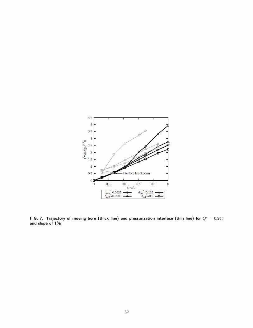
FIG. 7. Trajectory of moving bore (thick line) and pressurization interface (thin line) for Q∗ = 0.245and slope of 1%

32

0

1

2

3

4

5

6

7

0 1 2 3

Q*=0.245, dorif*=0.0625

0

1

2

3

4

5

6

7

h res

* =h r

es/D

Q*=0.245, dorif*=0.09375

0

1

2

3

4

5

6

7Q*=0.245, dorif

*=0.125

0 1 2 3

t*=t/(L/sqrt(gD))

Q*=0.368, dorif*=0.0625

Q*=0.368, dorif*=0.09375

Q*=0.368, dorif*=0.125

0 1 2 3

Q*=0.490, dorif*=0.0625

Q*=0.490, dorif*=0.09375

Q*=0.490, dorif*=0.125

Euler equation UAPH Exp rep 1 Exp rep 2

FIG. 8. Measured and predicted air phase pressures head for all tested conditions where dorif < 0.5 andslope 1%

33

0

1

2

3

4

5

6

7

0 1 2 3

Q*=0.245, dorif*=0.0625

0

1

2

3

4

5

6

7

h res

* =h r

es/D

Q*=0.245, dorif*=0.09375

0

1

2

3

4

5

6

7Q*=0.245, dorif

*=0.125

0 1 2 3

t*=t/(L/sqrt(gD))

Q*=0.368, dorif*=0.0625

Q*=0.368, dorif*=0.09375

Q*=0.368, dorif*=0.125

0 1 2 3

Q*=0.490, dorif*=0.0625

Q*=0.490, dorif*=0.09375

Q*=0.490, dorif*=0.125

Euler equation UAPH Exp rep 1

FIG. 9. Measured and predicted pressures at the pipe crown for x∗ = 0.39, dorif∗ < 0.5 and slope 1%

34

FIG. 10. Pipeline profile used by Vasconcelos et al. (2009) investigation

35

0

2

4

6

8

10

0 500 1000 1500 2000 2500 3000 3500 4000

head

(m

)

time (s)

MeasuredTraditional TPA

UAPHEuler equations

FIG. 11. Field measurements and predicted heads at the upstream ventilation valve of the water main

36

0

5

10

15

20

25

0 500 1000 1500 2000 2500 3000 3500 4000

head

(m

)

time (s)

MeasuredTraditional TPA

UAPHEuler equations

FIG. 12. Field measurements and predicted heads at the downstream ventilation valve of the watermain

37

0

0.01

0.02

0.03

0.04

0.05

0.06

0 500 1000 1500 2000 2500 3000 3500 4000

flow

rat

e ($

m3 /s

$)

time (s)

MeasuredTraditional TPA

UAPHEuler

FIG. 13. Field measurements and flow rates at the upstream ventilation valve of the water main

38