9th IAEA TM on H-mode Physics and Transport BarriersCatamaran Resort Hotel, San Diego

2003-09-25

Modeling of Transport Barrier Based on

Drift Alfven Ballooning Mode Transport Model

A. Fukuyama, M. Uchida and M. HondaDepartment of Nuclear Engineering,

Kyoto University, Kyoto 606-8501, Japan

Motivation

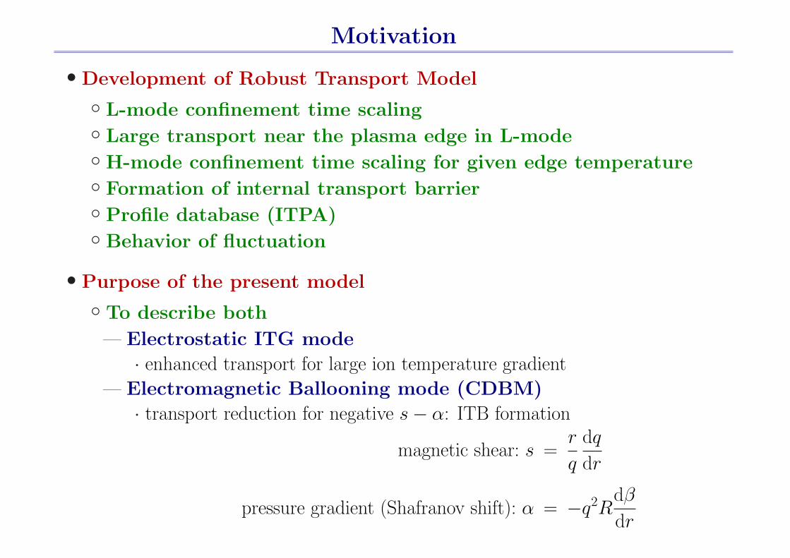
• Development of Robust Transport Model

L-mode confinement time scaling Large transport near the plasma edge in L-mode H-mode confinement time scaling for given edge temperature Formation of internal transport barrier Profile database (ITPA) Behavior of fluctuation

• Purpose of the present model

To describe both

— Electrostatic ITG mode

· enhanced transport for large ion temperature gradient

— Electromagnetic Ballooning mode (CDBM)

· transport reduction for negative s− α: ITB formation

magnetic shear: s =r

q

dq

dr

pressure gradient (Shafranov shift): α = −q2Rdβ

dr

Turbulent Transport Model

CDBMReduced MHD equation

ElectromagneticIncompressible

Toroidal ITG[hIon Fluid Equation

ElectrostaticBoltzmann Distribution of Electron

Drift Alfven Ballooning ModeReduced Two-Fluid Equation

ElectromagneticCompressible

• Small pressure gradient: Electrostatic ITG

• Large pressure gradient: Electromagnetic BM

• Without drift motion, it reduces to CDBM

• Ion parallel viscosity and compressibility desta-bilizes the mode

• s− α dependence similar to the CDBM mode

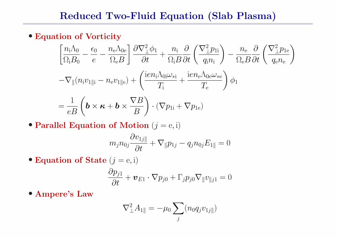
Reduced Two-Fluid Equation (Slab Plasma)

• Equation of Vorticity[niΛ0

ΩiB0− ε0

e− neΛ0e

ΩeB

]∂∇2

⊥φ1

∂t+

ni

ΩiB

∂

∂t

(∇2⊥p1i

qini

)− ne

ΩeB

∂

∂t

(∇2⊥p1e

qene

)

−∇‖(niv1‖i − nev1‖e) +

(ieniΛ0iω∗i

Ti+

ieneΛ0eω∗eTe

)φ1

=1

eB

(b× κ + b× ∇B

B

)· (∇p1i +∇p1e)

• Parallel Equation of Motion (j = e, i)

mjn0j

∂v1j‖∂t

+∇‖p1j − qjn0jE1‖ = 0

• Equation of State (j = e, i)

∂pj1

∂t+ vE1 · ∇pj0 + Γjpj0∇‖v‖j1 = 0

• Ampere’s Law

∇2⊥A1‖ = −µ0

∑j

(n0qjv1j‖)

Linear Analysis: Slab Plasma

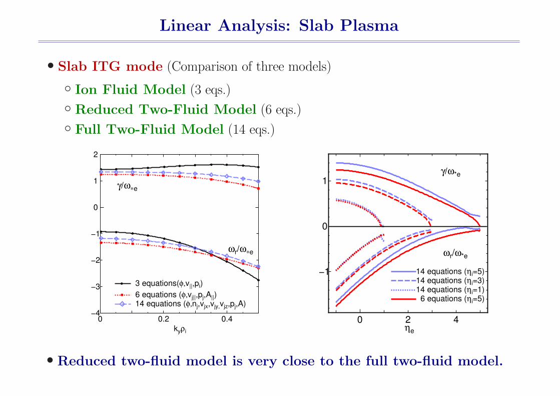
• Slab ITG mode (Comparison of three models)

Ion Fluid Model (3 eqs.)

Reduced Two-Fluid Model (6 eqs.)

Full Two-Fluid Model (14 eqs.)

0 0.2 0.4−4

−3

−2

−1

0

1

2

kyρi

ωr/ω∗e

3 equations(φ,v||,pi)

14 equations (φ,nj,vjx,vjy,vjz,pj,A)

γ/ω∗e

6 equations (φ,vj||,pj,A||)

0 2 4

−1

0

1

ηe

γ/ω*e

ωr/ω*e

14 equations (ηi=5)14 equations (ηi=3)14 equations (ηi=1) 6 equations (ηi=5)

• Reduced two-fluid model is very close to the full two-fluid model.

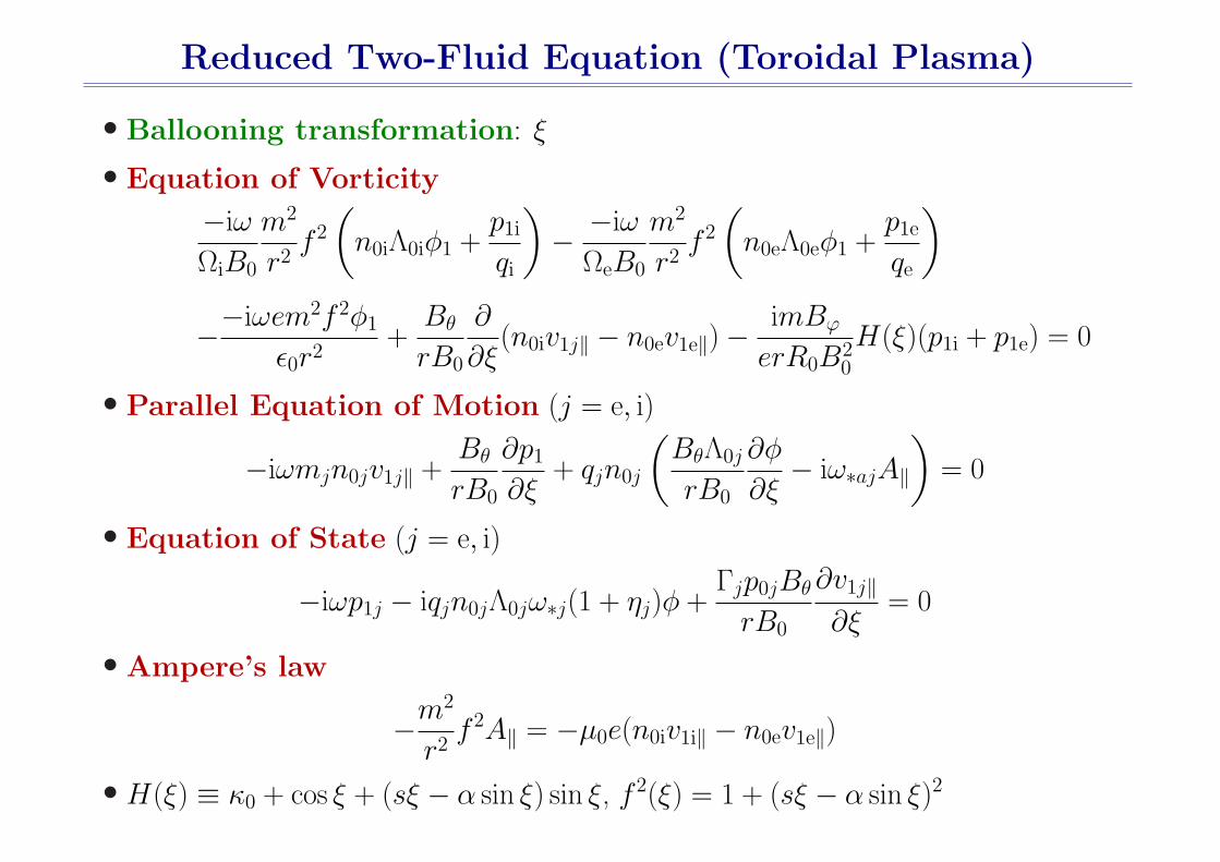
Reduced Two-Fluid Equation (Toroidal Plasma)

• Ballooning transformation: ξ

• Equation of Vorticity

−iω

ΩiB0

m2

r2f 2

(n0iΛ0iφ1 +

p1i

qi

)− −iω

ΩeB0

m2

r2f 2

(n0eΛ0eφ1 +

p1e

qe

)

−−iωem2f 2φ1

ε0r2+

Bθ

rB0

∂

∂ξ(n0iv1j‖ − n0ev1e‖)−

imBϕ

erR0B20

H(ξ)(p1i + p1e) = 0

• Parallel Equation of Motion (j = e, i)

−iωmjn0jv1j‖ +Bθ

rB0

∂p1

∂ξ+ qjn0j

(BθΛ0j

rB0

∂φ

∂ξ− iω∗ajA‖

)= 0

• Equation of State (j = e, i)

−iωp1j − iqjn0jΛ0jω∗j(1 + ηj)φ +Γjp0jBθ

rB0

∂v1j‖∂ξ

= 0

• Ampere’s law

−m2

r2f 2A‖ = −µ0e(n0iv1i‖ − n0ev1e‖)

• H(ξ) ≡ κ0 + cos ξ + (sξ − α sin ξ) sin ξ, f 2(ξ) = 1 + (sξ − α sin ξ)2

Linear Analysis: Toroidal Plasma

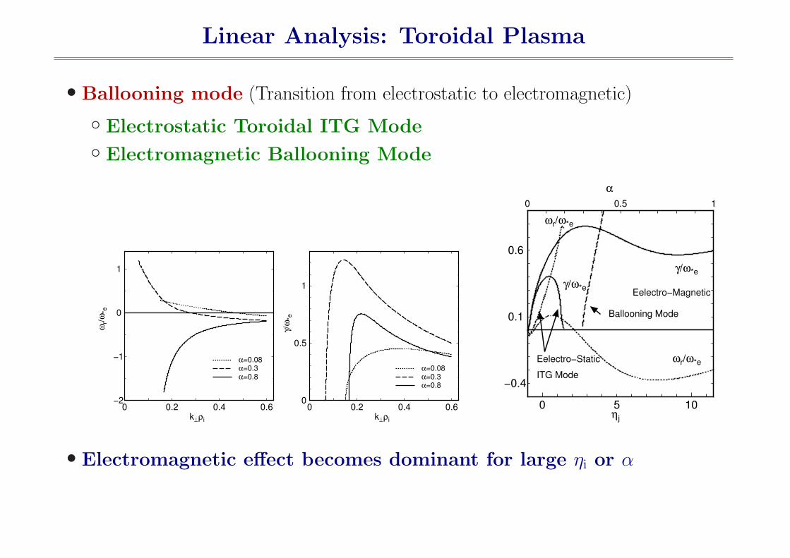
• Ballooning mode (Transition from electrostatic to electromagnetic)

Electrostatic Toroidal ITG Mode

Electromagnetic Ballooning Mode

0 0.2 0.4 0.6−2

−1

0

1

α=0.8α=0.3α=0.08

k⊥ρi

ωr/ω

*e

0 0.2 0.4 0.60

0.5

1

α=0.8α=0.3α=0.08

k⊥ρi

γ/ω

*e

0 5 10

−0.4

0.1

0.6

0 0.5 1

ηj

γ/ω*e

ωr/ω*e

Eelectro−Magnetic

Eelectro−Static

γ/ω*e

ωr/ω*e

α

Ballooning Mode

ITG Mode

• Electromagnetic effect becomes dominant for large ηi or α

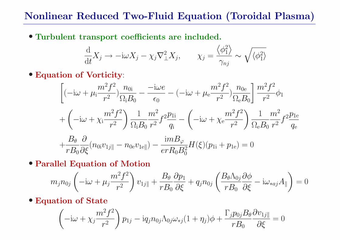
Nonlinear Reduced Two-Fluid Equation (Toroidal Plasma)

• Turbulent transport coefficients are included.

d

dtXj → −iωXj − χj∇2

⊥Xj, χj =

⟨φ2

1

⟩

γnj∼

√〈φ2

1〉

• Equation of Vorticity:[(−iω + µi

m2f 2

r2)

n0i

ΩiB0− −iωe

ε0− (−iω + µe

m2f 2

r2)

n0e

ΩeB0

]m2f 2

r2φ1

+

(−iω + χi

m2f 2

r2

)1

ΩiB0

m2

r2f 2p1i

qi−

(−iω + χe

m2f 2

r2

)1

ΩeB0

m2

r2f 2p1e

qe

+Bθ

rB0

∂

∂ξ(n0iv1j‖ − n0ev1e‖)−

imBϕ

erR0B20

H(ξ)(p1i + p1e) = 0

• Parallel Equation of Motion

mjn0j

(−iω + µj

m2f 2

r2

)v1j‖ +

Bθ

rB0

∂p1

∂ξ+ qjn0j

(BθΛ0j

rB0

∂φ

∂ξ− iω∗ajA‖

)= 0

• Equation of State(−iω + χj

m2f 2

r2

)p1j − iqjn0jΛ0jω∗j(1 + ηj)φ +

Γjp0jBθ

rB0

∂v1j‖∂ξ

= 0

• Ampere’s Law

−m2

r2f 2A‖ = −µ0e(n0iv1i‖ − n0ev1e‖)

• CDBM Eigenmode Equation

∂

∂ξ

γf

γ + ηrm2f + λm4f 2

∂φ1

∂ξ− (γ2f + γµm2f )φ1 +

αγ

γ + χm2fH(ξ)φ = 0

Marginal Stability Condition (γ = 0)

1

λ

∂2φ

∂ξ2− µm6f 3φ +

αm2f

χH(ξ)φ = 0

• Low β DABM Eigenmode Equation: Marginal Stability Condition

∂2φ

∂ξ2− µiχi

τ 2APc2m6f 3

r6ω2pi

φ +m2c2αi

2r2ω2pi

H(ξ)φ = 0

• Eigenmode equations for CDBM and DABM are similar.

Nonlinear Analysis (Toroidal Plasma)

• Amplitude Dependence of the Growth Rate

Linear growth rate (χj = 0) is sensitive to k⊥ρi.

For large α, electromagnetic effect becomes important.

Saturation level can be estimated from the marginal condition.

0 1 20

0.2

0.4

0.6

0.8

χj, µj [m2/s]

γ/ω

*e

(α=0.02, s=0.4, k⊥ρi=0.26)

(a)

0 1 20

0.1

µj, χj[m2/s]

γ/ω

*e

(α=0.02, s=0.4, k⊥ρi=0.36)

(b)

0 10 200

0.2

0.4

µj, χj[m2/s]

γ/ω

*e

DABM

ITGM

(α=0.2, s=0.4, k⊥ρi=0.11)

(c)

• Dependence on s and α

Transport of DABM is much larger than that of CDBM.

Negative magnetic shear reduces the transport.

χ is proportional to α3/2 for small α.

There exists critical α above which transport is strongly enhanced.

0 1

10−3

10−2

10−1

100

(α=0.01)

s

χ j, µ

j

[m2/s]

DABMCDBM

10−2 10−1 10010−1

100

101

102

s=0.8

α

χ js=0.4s=0.2s=−0.4(EM)s=−0.4(ES)

10−2 10−1 100

−1

0

1

s=0.8

α

ωr/ω

*e

s=0.4s=0.2s=−0.4s=−0.4

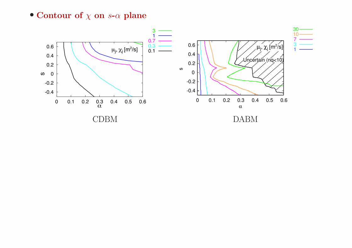
• Contour of χ on s-α plane

3 1

0.7 0.3 0.1

-0.4

-0.2

0

0.2

0.4

0.6

0 0.1 0.2 0.3 0.4 0.5 0.6

µj, χj [m2/s]

α

s

30 10 7 3 1

-0.4

-0.2

0

0.2

0.4

0.6

0 0.1 0.2 0.3 0.4 0.5 0.6α

s

Uncertain (nq<10)

µj, χj [m2/s]

CDBM DABM

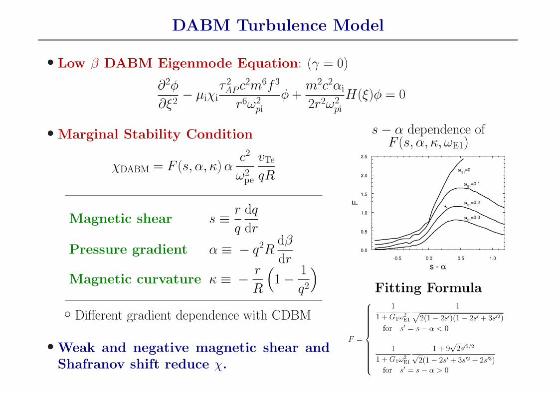
DABM Turbulence Model

• Low β DABM Eigenmode Equation: (γ = 0)

∂2φ

∂ξ2− µiχi

τ 2APc2m6f 3

r6ω2pi

φ +m2c2αi

2r2ω2pi

H(ξ)φ = 0

• Marginal Stability Condition

χDABM = F (s, α, κ) αc2

ω2pe

vTe

qR

Magnetic shear s ≡ r

q

dq

dr

Pressure gradient α ≡ − q2Rdβ

dr

Magnetic curvature κ ≡ − r

R

(1− 1

q2

)

Different gradient dependence with CDBM

• Weak and negative magnetic shear andShafranov shift reduce χ.

s− α dependence ofF (s, α, κ, ωE1)

0.0

0.5

1.0

1.5

2.0

2.5

-0.5 0.0 0.5 1.0

F ωE1

=0.2

ωE1

=0.3

ωE1

=0.1

ωE1

=0

s - α

Fitting Formula

F =

1

1 + G1ω2E1

1√2(1− 2s′)(1− 2s′ + 3s′2)

for s′ = s− α < 0

1

1 + G1ω2E1

1 + 9√

2s′5/2

√2(1− 2s′ + 3s′2 + 2s′3)

for s′ = s− α > 0

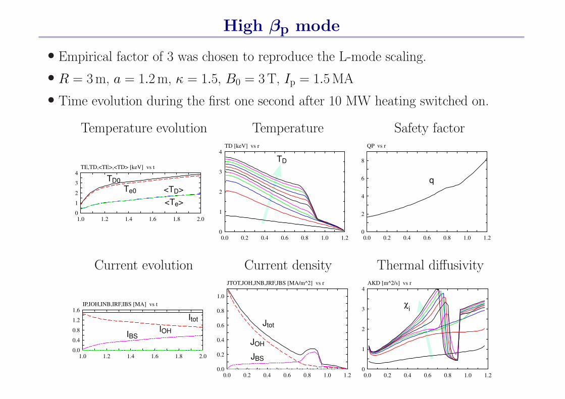
High βp mode

• Empirical factor of 3 was chosen to reproduce the L-mode scaling.

• R = 3 m, a = 1.2 m, κ = 1.5, B0 = 3 T, Ip = 1.5 MA

• Time evolution during the first one second after 10 MW heating switched on.

Temperature evolution Temperature Safety factor

TE,TD,<TE>,<TD> [keV] vs t

1.0 1.2 1.4 1.6 1.8 2.00

1

2

3

4TD0

Te0

<Te><TD>

TD [keV] vs r

0.0 0.2 0.4 0.6 0.8 1.0 1.20

1

2

3

4TD

QP vs r

0.0 0.2 0.4 0.6 0.8 1.0 1.20

2

4

6

8

q

Current evolution Current density Thermal diffusivity

IP,IOH,INB,IRF,IBS [MA] vs t

1.0 1.2 1.4 1.6 1.8 2.00.0

0.4

0.8

1.2

1.6Itot

IOHIBS

JTOT,JOH,JNB,JRF,JBS [MA/m^2] vs r

0.0 0.2 0.4 0.6 0.8 1.0 1.20.0

0.2

0.4

0.6

0.8

1.0

Jtot

JBS

JOH

AKD [m^2/s] vs r

0.0 0.2 0.4 0.6 0.8 1.0 1.20

1

2

3

4

χi

Summary

• In order to describe both the electrostatic ion temperature gradi-ent (ITG) mode and the electromagnetic current diffusive ballooningmode (CDBM), we have derived a set of reduced two-fluid equationsin both slab and toroidal configurations and numerically solved themas an eigenvalue problem.

• Linear analysis in a toroidal configuration describes a ballooningmode, which we call DABM (Drift Alfven Ballooning Mode).

Small pressure gradient: Toroidal ITG mode

Large pressure gradient: Ballooning mode with stabilizing ω∗

• Based on the theory of self-sustained turbulence, we have numeri-cally calculated the transport coefficients from the marginal stabilitycondition.

When α is small, χ is approximately proportional to α3/2.

χ is an increasing function of s−α; similar to CDBM model whichsuccessfully reproduces the ITB formation.

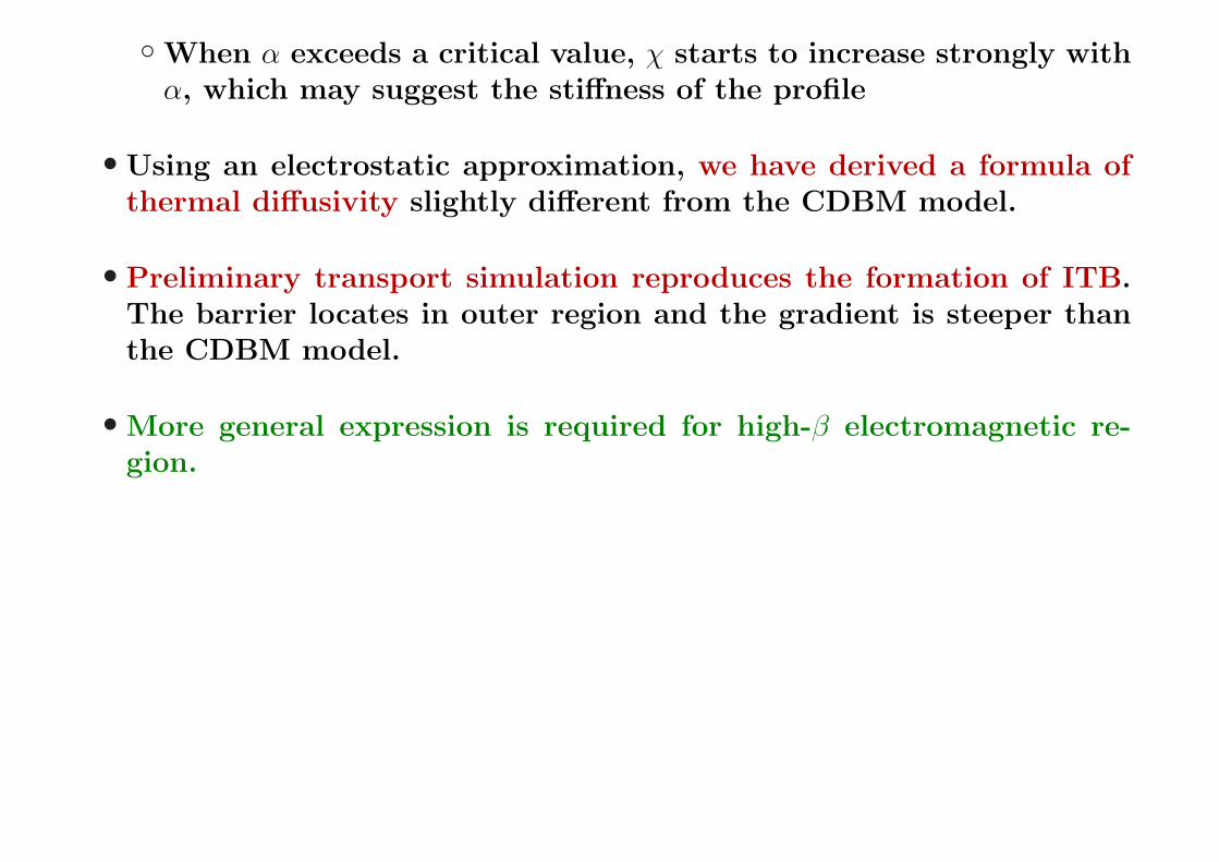
When α exceeds a critical value, χ starts to increase strongly withα, which may suggest the stiffness of the profile

• Using an electrostatic approximation, we have derived a formula ofthermal diffusivity slightly different from the CDBM model.

• Preliminary transport simulation reproduces the formation of ITB.The barrier locates in outer region and the gradient is steeper thanthe CDBM model.

• More general expression is required for high-β electromagnetic re-gion.

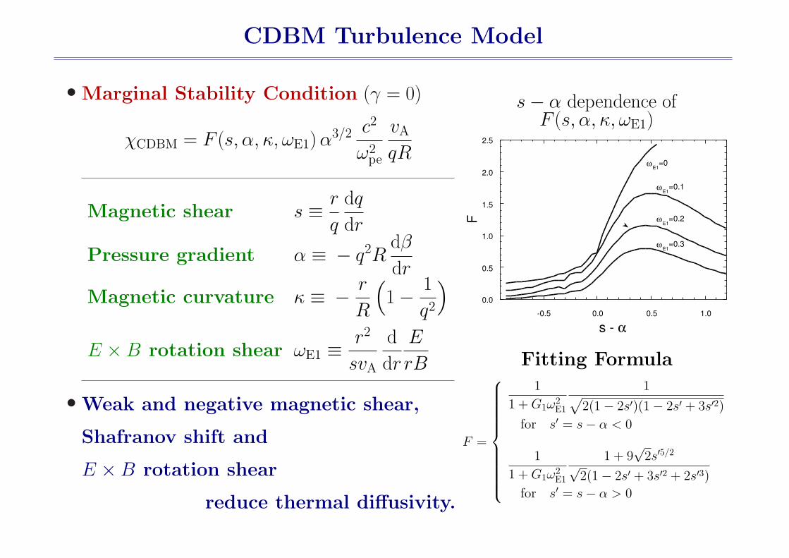
CDBM Turbulence Model

• Marginal Stability Condition (γ = 0)

χCDBM = F (s, α, κ, ωE1) α3/2 c2

ω2pe

vA

qR

Magnetic shear s ≡ r

q

dq

dr

Pressure gradient α ≡ − q2Rdβ

dr

Magnetic curvature κ ≡ − r

R

(1− 1

q2

)

E ×B rotation shear ωE1 ≡ r2

svA

d

dr

E

rB

• Weak and negative magnetic shear,

Shafranov shift and

E ×B rotation shear

reduce thermal diffusivity.

s− α dependence ofF (s, α, κ, ωE1)

0.0

0.5

1.0

1.5

2.0

2.5

-0.5 0.0 0.5 1.0

F ωE1

=0.2

ωE1

=0.3

ωE1

=0.1

ωE1

=0

s - α

Fitting Formula

F =

1

1 + G1ω2E1

1√2(1− 2s′)(1− 2s′ + 3s′2)

for s′ = s− α < 0

1

1 + G1ω2E1

1 + 9√

2s′5/2√

2(1− 2s′ + 3s′2 + 2s′3)for s′ = s− α > 0

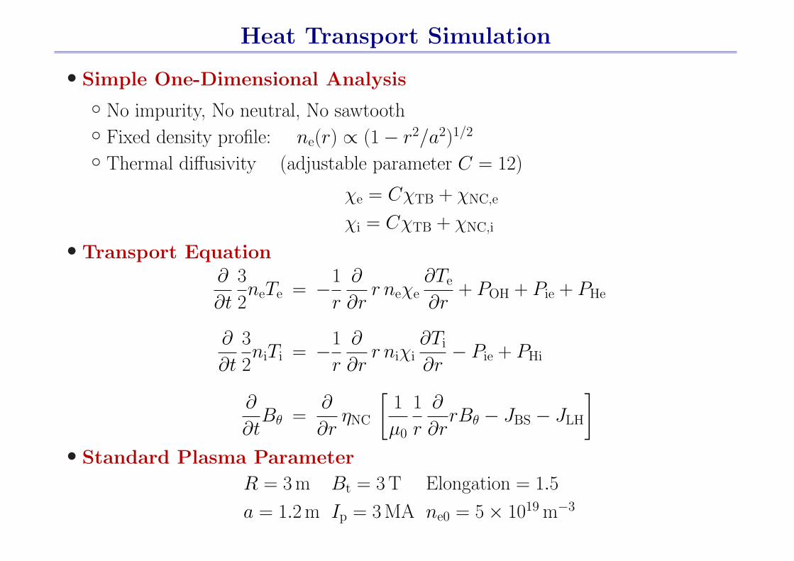
Heat Transport Simulation

• Simple One-Dimensional Analysis

No impurity, No neutral, No sawtooth Fixed density profile: ne(r) ∝ (1− r2/a2)1/2

Thermal diffusivity (adjustable parameter C = 12)

χe = CχTB + χNC,e

χi = CχTB + χNC,i

• Transport Equation∂

∂t

3

2neTe = −1

r

∂

∂rr neχe

∂Te

∂r+ POH + Pie + PHe

∂

∂t

3

2niTi = −1

r

∂

∂rr niχi

∂Ti

∂r− Pie + PHi

∂

∂tBθ =

∂

∂rηNC

[1

µ0

1

r

∂

∂rrBθ − JBS − JLH

]

• Standard Plasma Parameter

R = 3 m Bt = 3 T Elongation = 1.5

a = 1.2 m Ip = 3 MA ne0 = 5× 1019 m−3

High βp mode (1)

• R = 3 m, a = 1.2 m, κ = 1.5, B0 = 3 T, Ip = 1 MA

• Time evolution during the first one second after heating switched on

Temperater Current Safety factor

Te

T [k

eV]

r [m]0.0 0.2 0.4 0.6 0.8 1.0 1.2

0

2

4

6JTOT

J [M

A/m

2 ]r [m]

0.0 0.2 0.4 0.6 0.8 1.0 1.20.0

0.2

0.4

0.6

r [m]

q q

0.0 0.2 0.4 0.6 0.8 1.0 1.20

4

8

12

Shear Normalized Pressure Thermal diffusivity

s

s

r [m]0.0 0.2 0.4 0.6 0.8 1.0 1.2

0.0

0.5

1.0

1.5 α

α

r [m]0.0 0.2 0.4 0.6 0.8 1.0 1.2

0

1

2

3

4

χD

r [m]χ

[m2 /

s]

0.0 0.2 0.4 0.6 0.8 1.0 1.20

5

10

15

20

High βp mode (2)

• One second after heating power of PH = 20 MW was switched on

Temperater profile Current profile Safety factor

Te

TD

T [k

eV]

r [m]0.0 0.2 0.4 0.6 0.8 1.0 1.2

0

2

4

6JTOT

JOH

J [M

A/m

2 ]r [m]

JBS

0.0 0.2 0.4 0.6 0.8 1.0 1.2

0.0

0.2

0.4

0.6

r [m]

q q

0.0 0.2 0.4 0.6 0.8 1.0 1.20

4

8

12

Shear and pressure Thermal diffusivity s− α diagram

0.0 0.2 0.4 0.6 0.8 1.0 1.2

0

1

2

3

4

r [m]

s

α F(s,α)

s, α

, F(s

,α) χ

D

χTB

χNC

r [m]

χ [m

2 /s]

0.0 0.2 0.4 0.6 0.8 1.0 1.20

5

10

15

20

0 1 2 3 4 50.0

0.4

0.8

1.2

1.6

α

s before heating

1s after heating on

r=0m

r=0.6m

r=0.6m

r=1.2m

Simulation of Current Hole Formation

• Current ramp up: Ip = 0.5 −→ 1.0 MA

• Moderate heating: PH = 5 MW

• Current hole is formed.

• The formation is sensitive to the edge temperature.

.1*2+

./-*2+

.,0*2+

.*/+

-0

,0

.*/+

-0

,0

/.*0+

,1

-110.0*2+

1.-*2+

1,/*2+0./*1+

-2

,2

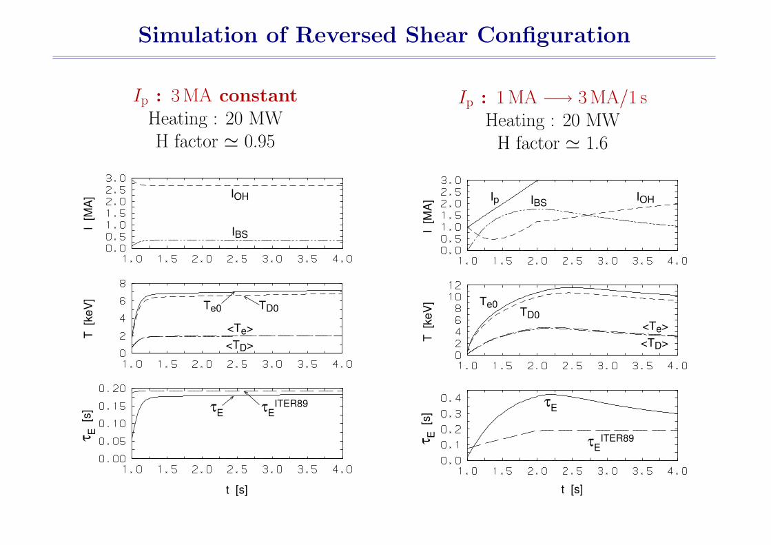
Simulation of Reversed Shear Configuration

Ip : 3 MA constantHeating : 20 MWH factor ' 0.95

I [M

A]

T [k

eV]

τ E [

s]

IBS

IOH

Te0 TD0

<Te><TD>

τE τEITER89

t [s]

Ip : 1 MA −→ 3 MA/1 sHeating : 20 MW

H factor ' 1.6

I [M

A]

T [k

eV]

τ E [

s]

Ip IBS IOH

Te0TD0

<Te><TD>

τE

τEITER89

t [s]

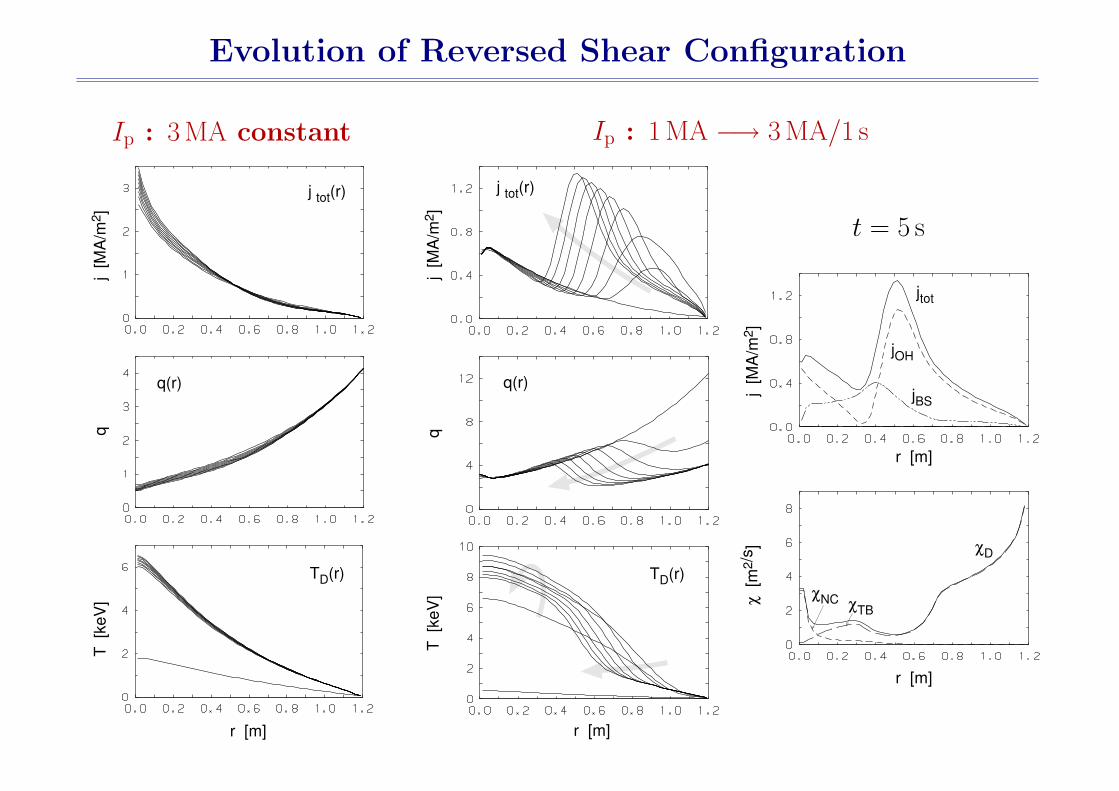
Evolution of Reversed Shear Configuration

Ip : 3 MA constant

j [M

A/m

2 ]T

[keV

]

j tot(r)

q(r)

TD(r)

r [m]

q

Ip : 1 MA −→ 3 MA/1 s

j [M

A/m

2 ]

j tot(r)

q(r)

TD(r)

T [k

eV]

r [m]

q

t = 5 s

j [M

A/m

2 ]χ

[m2/

s ]

jtot

jBS

jOH

r [m]

r [m]

χD

χTBχNC