MODELING OF REACTION KINETICS AND CHEMICAL REACTORS IN TRANSFORMATION OF BIOMASS

Johan Wärnå, Åbo Akademi

Laboratory of Industrial Chemistry and Reaction Engineering, Åbo Akademi

Reactormodelling

Catalysis

Kinetics

Aim with reactor and reaction kinetics modeling

Often the reaction routes, reaction kinetics and kinetic parameters are unknown

Combining Experimental work in

laboratory Mathematical modeling in

order to obtain a simulation tool for the design of reactors for the desired reaction

Scale up

ModelLab

Plant

Why do we need to know reactionkinetic parameters

Design of reactors Reaction rates determine the size or residence times

of the reactants Slow reaction longer residence time , larger

reactor

Biomaterial: Modelling works as beforebut what is new ?

Biomaterial More complex molecules from nature Mixture of molecules Often large molecules Diffusion influence makes a larger role (catalytic

reactions) A lot of properties have to be estimated or measured ?

Model building

Start with Literature studies Physical properties Derive some possible kinetic models and reaction paths

for your reaction A+B C+D 2X+Y Z Set up reactor model dc/dt=r Make experimental plan

Principles of reactor modelling

Kinetics and thermodynamics

Mass and heat-transfer Flow

REACTOR MODEL

Physicalproperties

Steps in reactor modelling

0 20 40 60 80 100 1200

10

20

30

40

50

60

70

A

B

E

F

IJ

Improve model

Moreexperiments

Fit of model toexperimental data

dcdt

rB= ⋅ρ

( )( )22

22

11

'

HHii

HjHAjj cKcK

ccKKkr

++=

∑

Reactor model

Reaction kineticsmodel

SoftwareModel solverParameter estimationMinimize object function

( )∑ −= ijestii wyyQ 2,exp,

Tid Volym ml C_syra mol/l0 427 7.55 426 7.3410 425 7.215 424 6.7830 423 6.3345 422 5.8260 421 5.7120 420 4.74180 419 4.034300 417 3.53360 416 3.38420 415 3.1261380 414 2.9

Experimental data

Reactor models

Homogeneous models One phase Gas or liquid Homogeneous catalyst

Heterogeneous Two or three phases Gas, liquid and solid catalyst

Three phase laboratory reactors

Basic Reactor Models

0 An 1An

Batch reactor

CSTRContinuos Stirred Tank Reactor

PFRPlug Flow Reactor

Batch

CSTR

PFR

ii r

dtdc

=

ii r

dtdc

=

iii rcc=

−τ

0

More complex reactor modelsWhat to include

Reaction anddiffusion

Reaction ?

Reaction ?

Gas-liquid solubilityMasstransfer

Porous catalystDiffusion

Three phase reactor model

GiLi

i

bLii

bGib

Li

kkK

cKcN 1+

−=

psLiv

bLi

R

Li aNaNdV

nd+=

•

vbLi

R

Gi aNdV

nd±=

•

2

2i ei i i

p ip

dc D d c dcs rdt dr r dr

ρε

= + +

Liquid phase

Gas phase

Gas-Liquid masstransfer

Reaction and diffusion incatalyst particle

ODE + PDE system

Experimental dataWhat to collect ?

Time Pressure Temp A B C D E pH 0 43.3 91 29.648 0.097 0.11 0.188 0 7.215 48.7 94 27.987 1.733 1.914 0.143 0 7.3220 48.6 92 22.583 5.353 2.628 0.167 0 7.0840 49.0 90 19.559 7.969 3.963 0.291 0 6.9360 50.0 90 17.847 9.762 3.772 0.066 0 6.79120 48.9 90 15.081 11.038 5.881 0.246 0 6.79180 52.5 90 12.284 12.956 6.31 0.321 0 6.73240 47.6 90 10.696 14.781 7.032 0.253 0 6.7300 48.9 90 8.334 15.558 7.412 0.327 0 6.54

Collect all possible data from your experimentsIt can be used in the model

Software for estimation of reaction kinetic parameters and reactor modelling

Parameter estimation Simulation Sensitivity Optimization

Athena Visual Studio

Modest

Software

Modest Windows or Linux Fortran compiler Intel Visual Fortran Gfortran

2 versions Windows user interface Text input file (Linux and

Windows) MCMC

Additional graphics with Matlab

Athena Visual Studio Windows Fortran compiler Intel Visual Fortran G95

Other optionsMatlabOctave (open source)Process simulator

AspenPro II

The models are not in the programsThe user has to write the program code for the modelsBasic programming skills needed !

Mathematical methodsNumerical solvers in the software

Algebraic model Non linear equation model (NLE) NLE (Non Linear Equation Systems) Newton-Raphson method Ordinary differential equation model (ODE) Backward

difference method PDE solver

Optimization and parameter estimation Simflex and/or Levenberg-Marquardt methods

Estimation of parameters and their distributions in models Markow Chain MonteCarlo MCMC

Examples

Estimation resultsk=0.042745285K=3.020598Ea=58593.68

0 500 1000 15002

3

4

5

6

7

8

60 C

70 C

Time

c

Two experiments at60 ºC and 70 ºC

Batch reactordc/dt=mcat*rate

Esterification results

Acid + Alcohol -> Ester + Water

r k e c cK

c ci

ER T T

A Beq

c D

A

medel= −

−−

1 1 1

Results, statisticsTotal SS (corrected for means) 0.8183E+02Residual SS 0.8513E+00Std. Error of estimate 0.1631E+00Explained (%): 98.96

The Hessian:

0.167E+05 0.312E+02 0.189E-030.312E+02 0.619E+00 -0.274E-070.189E-03 -0.274E-07 0.138E-08

Estimated Estimated Est. Relative Parameter/Parameters Std Error Std Error (%) Std. Error

0.453E-01 0.133E-02 2.9 34.10.306E+01 0.218E+00 7.1 14.00.708E+05 0.440E+04 6.2 16.1

The covariances of the parameters:

0.176E-05-0.891E-04 0.475E-01-0.243E+00 0.131E+02 0.193E+08

The correlation matrix of the parameters:

1.000-0.308 1.000-0.042 0.014 1.000

Sensitivity analysis: Did we find the best values for the estimated parameters

Vary one parameterAnd keep the otherParameters at fixed values

Calculate Sum of square error

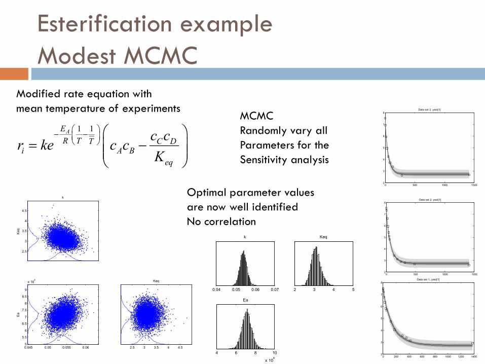
Esterification example: Modest MCMC (Markow Chain Monte Carlo)

0 500 1000 15002

4

6

8 data set 1

0 500 1000 15002

4

6

8 data set 2

0 500 1000 15002

4

6

8 data set 3

2.5

3

3.5

4

4.5

Keq

k

0 5 10 15 20

x 109

6.6

6.8

7

7.2

7.4

7.6

x 104

Ea

2.5 3 3.5 4 4.5

Keq

0 0.5 1 1.5 2

x 1010

k

2 3 4 5

Keq

6.5 7 7.5 8

x 104

Ea

AEC DRT

i A Beq

c cr ke c cK

− = −

Fit of model to experimentaldata looks good

Optimal values forparameters arenot well identified

Correlation betweenEA and k

Rate equation

Esterification exampleModest MCMC

2.5

3

3.5

4

4.5

Keq

k

0.045 0.05 0.055 0.065

5.5

6

6.5

7

7.5

8

8.5

9

x 104

Ea

2.5 3 3.5 4 4.5

Keq

0.04 0.05 0.06 0.07

k

2 3 4 5

Keq

4 6 8 10

x 104

Ea

0 500 1000 15002

3

4

5

6

7

8Data set 3, yest[1]

0 500 1000 15002

3

4

5

6

7

8Data set 2, yest[1]

0 200 400 600 800 1000 1200 14002

3

4

5

6

7

8Data set 1, yest[1]

1 1AER T T C D

i A Beq

c cr ke c cK

− −

= −

Optimal parameter valuesare now well identifiedNo correlation

Modified rate equation with mean temperature of experiments

MCMCRandomly vary allParameters for theSensitivity analysis

Modeling and Scale-up of Sitosterol Hydrogenation Process: from laboratory slurry reactor to plant scale

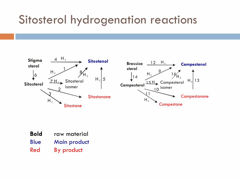
Sitosterol hydrogenation reactions

Sitosterol

Sitostanol

Sitostanone

Sitostane

H 2

1

23

Stigmasterol

H 24

H 2

Sitosterolisomer

H 2

H 2

H 25

8

76

Campesterol

Campestanol

Campestanone

Campestane

H 29

1011

Brassicasterol

H 212

H 2

Campesterolisomer

H 2

H 2

H 213

16

1514

Bold raw materialBlue Main productRed By product

Model for Sitosterol hydrogenationIdea

Feedstock from natural sources (always different composition) Set up reaction kinetics model Reactor model for laboratory reactor Reactor model for plant reactor (10 m3)

For every new feedstock make laboratory experiments and estimate reaction kinetic parameters

Simulate the plant reactor with the new parameters

Kinetic model and reactor model

( )( )22

22

11

'

HHii

HjHAjj cKcK

ccKKkr

++=

∑

Based on this mechanistic hypothesis, the rates of the hydrogenation steps become:

DD

ccKKk=r

H

HAHA

2

211

2 D

cKk=r AA22

DD

ccKKk=r

H

HAHA

2

233

2

DD

ccKKk=r

H

HJHJ

2

244

2 DD

ccKKk=r

H

HCHC

2

255

2 DD

ccKKk=r

H

HJHJ

2

266

2

DD

ccKKk=r

H

HAHA

2

277

2 DD

ccKKk=r

H

HKHK

2

288

2 DD

ccKKk=r

H

HEHE

2

299

2

DcKk=r EE10

10 DD

ccKKk=r

H

HEHE

2

21111

2 DD

ccKKk=r

H

HIHI

2

21212

2

DD

ccKKk=r

H

HGHG

2

21313

2 DD

ccKKk=r

H

HIHI

2

21414

2

where D and DH2 are defined as

KKJJIIGG

FFEEDDCCBBAA

cKcKcKcKcKcKcKcKcKcK=D

++++++++++1

2221 HHH cK= D +

ibi rρ=

dtdc

bHvHH ρraN=

dtdc

+

− H

GvlvH c

KRTPak=aN /

ρB catalyst bulk density =mcat/VliqNH flux of hydrogen from gas to liquidK gas-liquid equilibrium constantkl gas-liquid mass transfer coefficientr reaction rate

Liquidphase

• Catalyst 1, Raw material 1– Temperatures 70ºC, 95 ºC and 120 ºC– Pressure 4, 7, 9.5 bar– Catalyst amount 2.9 g– 9 data sets

• Catalyst 2, Raw material 2– Temperatures 70ºC, 95 ºC and 120 ºC– Pressure 15, 30, 45 bar– Catalyst amount 1.25 g– 9 data sets

Experiments performed in laboratory reactor

Experiment 1-9Catalyst 1

Explained 99.82 %

Experiment 10-18Catalyst 2

Explained 99.06 %

Parameter value Std. Error(%) Parameter value Std. Error(%)

k1 (mol/ m3min) 274 13.9 548 34.1

k2 (mol/ m3min) 7.51 14.2 25.2 28.7

k3 (mol/ m3min) 1.93 17.3 57.1 23.9

k6 (mol/ m3min) 15.5 5.8 421 21.2

k7 (mol/ m3min) 2.95 19 1470 30.6

k8 (mol/ m3min) 0.0109 53.1 5.37 19.2

k9 (mol/ m3min) 259 13.9 1660 18.9

k10 (mol/ m3min) 12.2 15.1 39.9 26.8

k11 (mol/ m3min) 0.761 27.7 0.0607 68.5

k14 (mol/ m3min) 44.4 24.8 2970 34.4

ΔEA1 (J/mol) 57000 2.8 74100 5.2

ΔEA2 (J/mol) 95300 3.4 55200 20.9

ΔEA3 (J/mol) 124000 3.8 98000 9.5

ΔEA6 (J/mol) 43700 4.8 80100 6.1

ΔEA7 (J/mol) 99900 10 84400 5.3

ΔEA8 (J/mol) 27500 36.3 41200 5.7

KA (m3/mol) 0.000776 19.6 0.00161 29

KB (m3/mol) 0.718 20.1 6.51 26.2

KJ (m3/mol) 0.0186 12.5 0.0147 26.1

KK (m3/mol) 0.0618 38.2 4.87 21

KH2 (m3/mol) 0.275 11.1 0.0562 15.1

ΔH2 (J/mol) 18600 25.2 3440 58.3

0 20 40 60 80 100 1200

10

20

30

40

50

60

70

A

B

E

F

IJ

0 20 40 60 80 100 120

0

0.5

1

1.5

2

2.5

3

3.5

4

4.5

5

GH

CDK

Dataset 1, exp 5, 7 bar, 70°C

0 5 10 15 20 25 30 35 40 45 50 0 5

10 15 20 25 30 35 40 45 50

Experimental

Est

imat

ed

Sitosterol

0 0.5 1 1.5 2 2.5 3 3.5 4 4.5 50

0.5

1

1.5

2

2.5

3

3.5

4

4.5

5Sitostanone

Experimental

Est

imat

ed

Fit of model to experiments

0 20 40 60 80 100 1200

10

20

30

40

50

60

70

A

B

E

F

IJ

0 20 40 60 80 100 1200

0.5

1

1.5

2

2.5

3

3.5

4

4.5

5

G

H

C

D

K

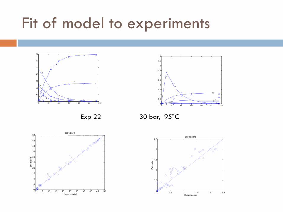
Exp 22 30 bar, 95°C

0 5 10 15 20 25 30 35 40 45 50 0 5

10 15 20 25 30 35 40 45 50

Experimental

Est

imat

ed

Sitosterol

0 0.5 1 1.5 2 2.5 0

0.5

1

1.5

2

2.5

Experimental

Est

imat

ed

Sitostanone

Fit of model to experiments

100 200 300 400 5000

1

2

3x 10

4

k1 0 5 10 15 20

0

500

1000

1500

2000

k2

0 2 4 60

500

1000

1500

2000

k3 0 10 20 30 40

0

0.5

1

1.5

2x 10

4

k6

Sensitivity plots: Check that parameters are well identified

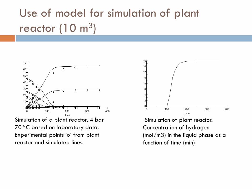
Use of model for simulation of plant reactor (10 m3)

0 10 20 30 40 50 60 70

0 100 200 300 400 time

Simulation of a plant reactor, 4 bar 70 °C based on laboratory data. Experimental points ‘o’ from plant reactor and simulated lines.

0 2 4 6 8

10 12 14 16

0 100 200 300 400 time

Simulation of plant reactor. Concentration of hydrogen (mol/m3) in the liquid phase as a function of time (min)

Reaction and diffusion: LactoseHow are by products formed Lactose is inexpensive There is a lot of lactose (by-product of cheese manufacturing) Lactose intolerance is common Lactose can be isomerized Lactose can be oxidized Lactose can be hydrogenated Lactitol is a sweetening agent Lactulose is a laxative Lactobionic acid is an organ preserving liquid

Lactulose

Lactobionicacid

SorbitolGalactitol

O O OHOH

OHHO

OHOH

OH

O O OHOH

OHHO

OHOH

OH

Lactulitol

Lactitol

+

Alternative reaction schemes

Alternative 2

Alternative 1

Experiments + linear plots

Effect of catalyst amount Effect of hydrogen pressure

Linear plots rate constant

How are By-products formed

The behaviour of by-products is complicated It can be revealed with yield-conversion plots how

sorbitol and galactitol are formed ?

0 50 100 150 200 250 3000

5

10

15

20

25

30

35

40

45

time (min)

w-%

20 bar

20 bar

70 bar

70 bar

0 50 100 150 200 250 3000

0.1

0.2

0.3

0.4

0.5

time (min)

w-%Preliminary data fit

Main products ok By products bad

Alternative reaction schemes in brief

Alternative 1

Lactose → lactitol → sorbitol+galactitol (1,5)Lactose → lactulose → lactulitol (2,4)Lactose ↔ lactobionic acid (3)

Alternative 2

Lactose → lactitolLactose → lactulose -> lactulitolLactose ↔ lactobionic acidLactose → sorbitol + galactitol

Mass balances, rate equationsand yield

Bjiji r

dtdc ρν∑= ( )( )ll

nHHH

nHHAj

j cKcK

cckR

∑++=

11 22

22

2

AckR 11 '=AckR 22 '=

DA ckckR 333 '' −−=CckR 44 '=BckR 55 '=

)))'''(exp(/ 3210 tkkkcc BAA ρ++−=

))'exp()''))(exp('''/('(/ 5510 tktkkkkcc BBAB ρρ −−−−=))'exp()''))(exp('''/('(/ 4420 tktkkkkcc BBAC ρρ −−−−=

))''exp(1)(''/'(/ 30 tkkkcc BAD ρ−−=))'exp(1)('/1()''exp(1)(''/1))(('''/()''(/ 444410 tkktkkkkkkcc BBAE ρρ −−−−−−=))'exp(1)('/1()''exp(1)(''/1))(('''/()''(/ 555510 tkktkkkkkkcc BBAF ρρ −−−−−−=

)**)1()1)((1/(/ 5510 ααα XXcc AB −−−−=)**)1()1)((1/(/ 4420 ααα XXcc AC −−−−=

Xcc AD 30/ α=)1**)1()(1/(/ 44420 −−+−= αααα XXcc AE)1**)1()(1/(/ 55510 −−+−= αααα XXcc AF

Improved data fitting results

0 50 100 150 200 2500

5

10

15

20

25

30

35

40

Lactose

Time (min)Galactitol & Sorbitol

Lactitol

W-%

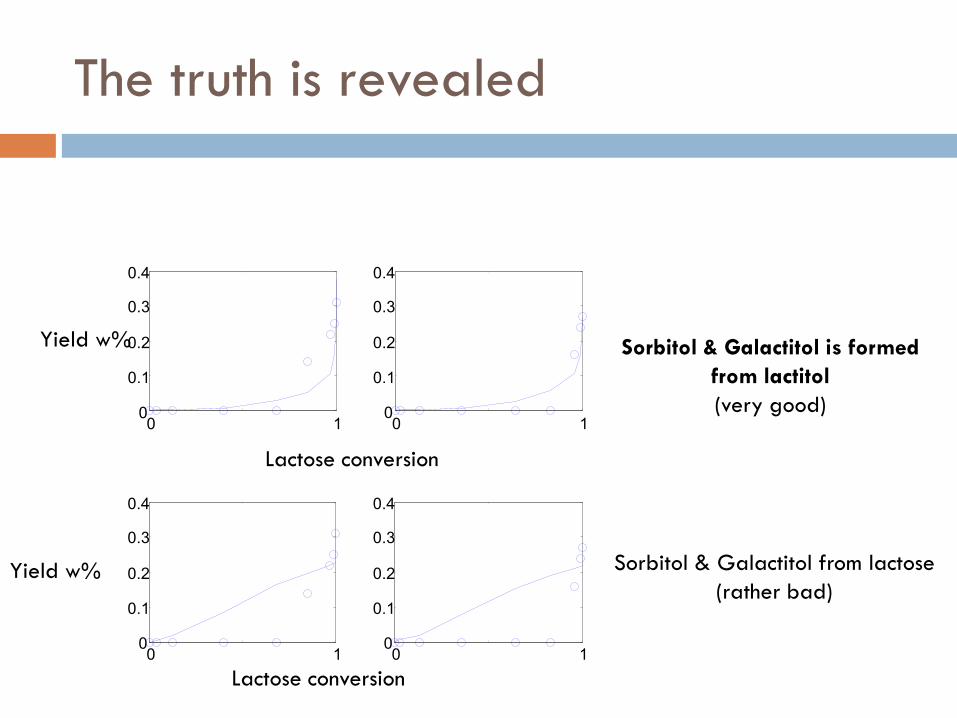
The truth is revealed

0 10

0.1

0.2

0.3

0.4

0 10

0.1

0.2

0.3

0.4

0 1 0

0.1

0.2

0.3

0.4

0 1 0

0.1

0.2

0.3

0.4

Sorbitol & Galactitol from lactose(rather bad)

Sorbitol & Galactitol is formedfrom lactitol(very good)

Yield w%

Yield w%

Lactose conversion

Lactose conversion

Particle model

( )

−= −

drrNdrr

dtdc S

iSpip

i ρε 1

∑=j

jjiji aRr ν

Reaction, diffusion and catalyst deactivation in porous particles

Particle model

Rates

Lactose hydrogenation

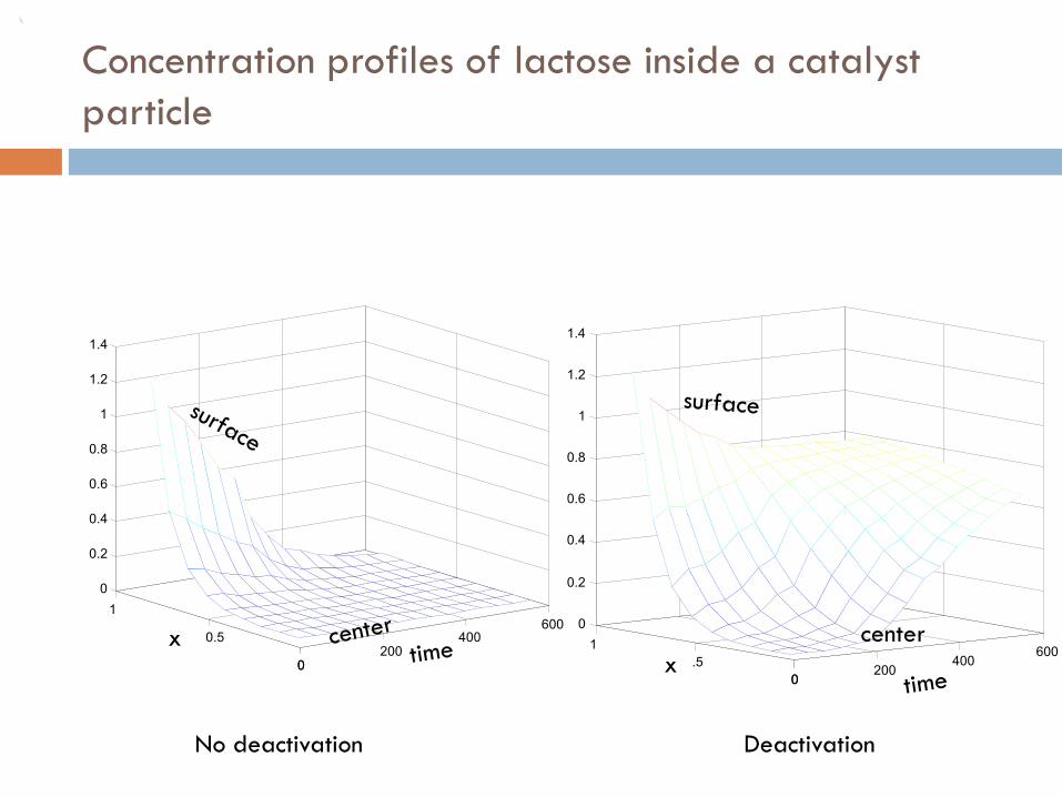
Concentration profilesInside catalyst particleWith different particle sizes

SurfaceCenter

LactuloseLactulitol

0 0.1 0.2 0.3 0.4 0.5 0.6 0.7 0.8 0.9 10

1

2

3

4

5

6

7x 10

-3

x

c (m

ol/l)

0.03 mm

0.03 mm

0.3 mm0.3 mm

1.0 mm

1.0 mm

3.0 mm

3.0 mm

0200

400600

0

0.5

10

0.2

0.4

0.6

0.8

1

1.2

1.4

0200

400600

0.5

10

0.2

0.4

0.6

0.8

1

1.2

1.4

Concentration profiles of lactose inside a catalyst particle

No deactivation Deactivation

centerxx

Production of DMC Dimethylcarbonate

•DMC•Methylating and carbonylatingagent•Biodegradable•Gasoline additive – replacingMTBE•Electrolyte in lithium batteries

DMC model

DMC

MeOH CO2

r1=k1*cA*cBr2=k2*cC*cwaterr3=k3*cE*cWaterr4=k4*cC*cFr5=k5*cG*cAr6=k6*cB*cEr7=k7*cE*cAr8=k8*cH*cBr9=k9*cH*cWater! Batch reactor modelds(1)=-2.0d0*r1-2.0d0*r5-r7+r2

+2.0d0*r4 ! metanolds(2)=-r3-r6-r7 ! butylenoxideds(3)= -r1+r2-r8 ! CO2ds(4)= r5+r8-r5+r4 ! But carbonateds(5)= r1-r2+r5-r4 ! DMCds(6)= r7-r8-r9

Wood chip

2D dynamic model Reaction Diffusion Structural changes during

reaction: porosity changes

Most complex model we havemade !

Conclusions

More and more complex molecules and mixtures from the nature enter the arena

Development of new catalyst and reactortechnologies is the key issue for betterprocesses and products

Mathematical modelling should cover allaspects: kinetics, mass transfer, flow modellingto process modelling – in a balanced way

But keep the models as simple as possible

Teknisk kemi och reaktionsteknik

Åbo Akademi

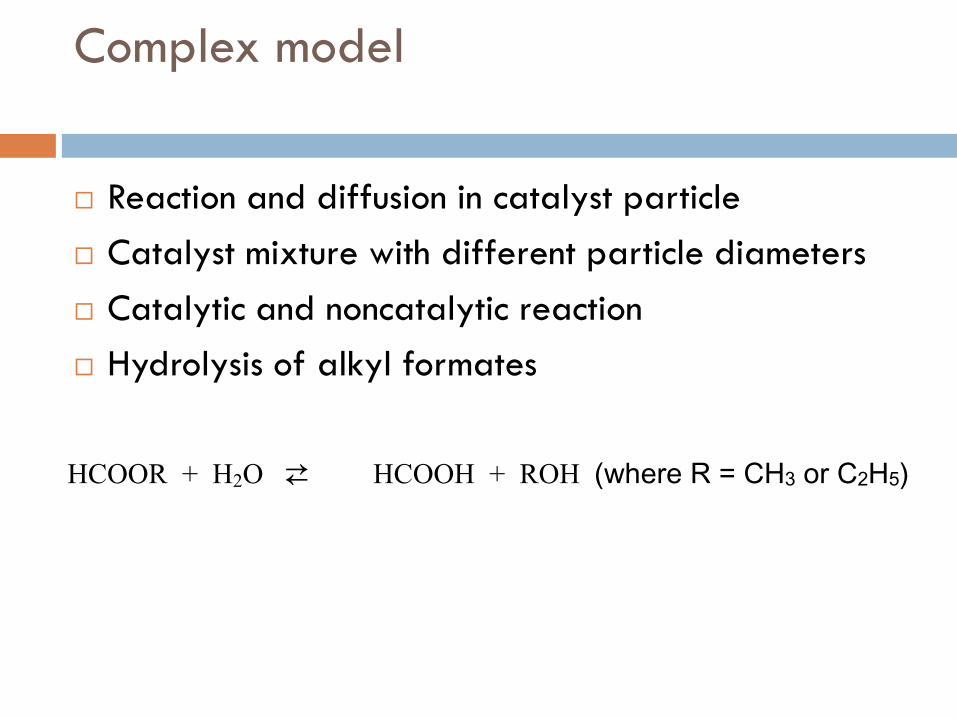
Complex model

Reaction and diffusion in catalyst particle Catalyst mixture with different particle diameters Catalytic and noncatalytic reaction Hydrolysis of alkyl formates

HCOOR + H2O ⇄ HCOOH + ROH (where R = CH3 or C2H5)

Reactor and kinetic model

Catalyst particle Reaction+diffusion

Batch reactor Catalyst particles of

different sizes

Reaction kinetics

2cat,i P eii i i

noncat,i 2 2P P j

rρ DdC d da-1rdtε R dX X dX

C Cε

= + + +

dC 2i a y N xp j ij jdt j

noncatr= +∑

C DA B

eq

c cr k c cK

= −

1 1

0

AER T Tk k e − − =

1 1

0,ref

HR T T

eq eqK k e ∆

− − =

0

2

4

6

8

10

12

14

16

18

58.9

-68.

2

68.2

-79.

1

79.1

-91.

7

91.7

-106

106-

123

123-

143

143-

165

165-

192

192-

222

222-

258

258-

299

299-

346

346-

401

401-

465

465-

539

539-

625

625-

724

724-

840

840-

973

973-

1128

Diameter range (µm)

%

Mathematical model

Ordinary differential model (ODE) Partial Differential Model (PDE)

Backward difference Convert PDE to ODE:s by method of lines

Model code

where (s < 0.0d0 ) s=1.0d-10catrad=catrad/100 ! radius in dm

if (iobs.lt.nobs.and.t.gt.0.0d0) then t1=xdata(1,iobs) ! timet2=xdata(1,iobs+1)Te1=xdata(2,iobs)Te2=xdata(2,iobs+1)Temp=Temp+(Te2-Te1)/(t2-t1)*(t-t1)end ifVolume=Volume-float(iobs-1)*5.0d0

Temp=Temp+273.15d0 do k=1,ndistidist=(k-1)*ncom*npcat

nmax=npcat+1! call discr(npcat,2,4,nmax,discr_points,discr_int,ierr)

call diffusion(poro,tortu,temp,diff)

ap=(shape+1.0d0)*mcat/volume/catrad(k)/rhop

rhob=mcat/volume /1.0d-3! calculate concentration profile inside catalyst particle

nd=maxptsdo i=1,ncom

ix=ncom+1+(i-1)*npcat +idist

ib1 = 2 ! centerib2 = 1 ! surface

ind = 1 !3

index=0call deriv1(ind,ib1,ib2,nd,npcat,ndp2,nmax,index,h,

& s(ix),dc1(ix),dum,ierr)

call rates(conc,ratehet,ratehom,xdata,gpar, ngpar,& lpar, nlpar,nx,nobs,iobs,iset)

xpos=dfloat(j-1)/dfloat(npcat-1)! xpos=discr_points(j)

do i=1,ncom! print *,i,j,conc(i),ratehet(i)

dpr2=diff(i)/poro/catrad(k)/catrad(k)

icat=ncom+j+(i-1)*npcat+idistil=i ! bulk concentration

if (j.eq.npcat) then ! surface of catalyst! ds(icat)=dc1(icat)+kla*catrad(k)/diff(i)*(s(il)-s(icat)) ! slurry reactor

ds(icat)=dc1(icat)+kla*(s(il)-s(icat)) ! slurry reactorelse if (j.eq.1) then ! center of catalyst particle

ds(icat)= 1.0d2*dc1(icat)else

! ds(icat)=dpr2*dc2(icat)+dpr2*shape/xpos* ! & dc1(icat)+rhop/poro*cratehet(i)

ds(icat)=dpr2*dc2(icat)+dpr2*shape/xpos* & dc1(icat)+rhop/poro*ratehet(i)+ratehom(i)

! print *,i,conc(i),ratehet(i),dpr2,diff(i)end if

rate_het_particle(i,j,k)=ratehet(i)+ratehom(i)

end do! pause

end do

end do ! k

if (ierr.ne.0) thenwrite(*,*)'error from deriv ',ierrstop

end if

dum(1)=0.0d0avnlpi(1:ncom)=0.0d0

do i=1,ncomdo k=1,ndist

do j=2,npcat

Complex modelMore time neededTo write model code

Concentration inside catalyst particle for different particle sizes (mm)

0 0.1 0.2 0.3 0.4 0.5 0.6 0.7 0.8 0.9 17

7.2

7.4

7.6

7.8

8

8.2

x

c m

ol/d

m3

1.1

0.9

0.79

0.68

0.58

0.50.44

0.370.32

0.15

Catalystparticle

Fit of model to experimental data

0 50 100 1500

0.5

1

1.5

time (min)

mol

1g

0 50 1000

0.5

1

1.5

time (min)

mol

2.5g

0 50 1000

0.5

1

1.5

time (min)

mol

5g

0 50 1000

0.5

1

1.5

time (min)

mol

10g

Kinetic model

1

11 1 9 2

zHMRr k K pH c θ +=

2

12 4 9 2

zHMRr k K pH c θ +=

13 3 HMRr k c=

24 4 HMRr k c=1

5 5 9 2z

MATr k K pH c θ += ( ) ( )1 26 7 8 9 2 1zHMR HMR MATf k c k c c K pHθ θ θ θ= + + + + −

( )( )1 'i i

ffθ

θ θθ+ = +

( ) ( )1 2

16 7 8 9 2' 1 z

HMR HMR MATf k c k c k c z K pHθ θ −= + + + +

Where the coverage is obtained from

The coverage can be solved iteratively with the Newton-Raphson method

The derivative is

ExampleMCMC

Reactions 1 HMR_1 → MAT 2 HMR_2 → MAT 3 HMR_1 → prop_MAT_1 4 HMR_2 → prop_MAT_2 5 MAT → BP

Modest code

do i=1,1000fun=theta+kk*

1 theta**z+sqrt(K9*pH2)*theta-1.0d0funp=1.0d0+kk*z*theta**(z-1.0d0)+sqrt(K9*pH2)

theta1=theta-fun/funp! print *,i,theta,theta1,fun,funp

if (abs(theta1-theta).lt.1.0d-5) then ! convergedtheta=theta1 goto 20

end iftheta=theta1if (i.gt.999) thenprint *,'max iterations reached 1000 ',theta,theta1stop

end if end do ! iterate again

rhoB=mcat/vol/1.0d-3 ! gram/liter

r1=k1*sqrt(K9)*cHMR1*sqrt(pH2)*theta**(z+1.0d0)r2=k2*sqrt(K9)*cHMR2*sqrt(pH2)*theta**(z+1.0d0)r3=k3*cHMR1 r4=k4*cHMR2 r5=k5*sqrt(K9)*cMAT*sqrt(pH2)*theta**(z+1.0d0)

ds(1)=(-r1-r3)*rhoB ! cHMR1ds(2)=(-r2-r4)*rhoB ! cHMR2ds(3)=(r1+r2-r5)*rhoB ! cMATds(4)= r3*rhoB ! cP1ds(5)= r4*rhoB ! cP2ds(6)= r5*rhoB ! cB

Find coverage

Kinetic and reactor model

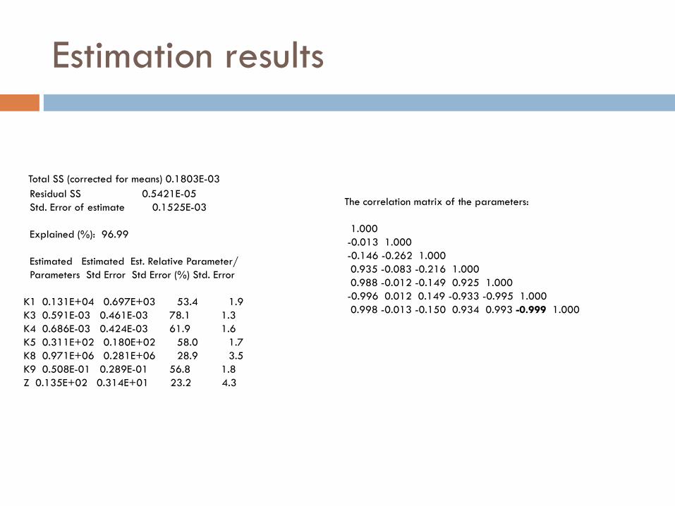
Estimation results

Total SS (corrected for means) 0.1803E-03Residual SS 0.5421E-05Std. Error of estimate 0.1525E-03

Explained (%): 96.99

Estimated Estimated Est. Relative Parameter/Parameters Std Error Std Error (%) Std. Error

K1 0.131E+04 0.697E+03 53.4 1.9K3 0.591E-03 0.461E-03 78.1 1.3K4 0.686E-03 0.424E-03 61.9 1.6K5 0.311E+02 0.180E+02 58.0 1.7K8 0.971E+06 0.281E+06 28.9 3.5K9 0.508E-01 0.289E-01 56.8 1.8Z 0.135E+02 0.314E+01 23.2 4.3

The correlation matrix of the parameters:

1.000-0.013 1.000-0.146 -0.262 1.0000.935 -0.083 -0.216 1.0000.988 -0.012 -0.149 0.925 1.000

-0.996 0.012 0.149 -0.933 -0.995 1.0000.998 -0.013 -0.150 0.934 0.993 -0.999 1.000

MCMC, sensitivity analysis

0

5

10

15x 10

-4

2

1

0

5

10x 10

-4

3

2

20

40

60

4

3

5

10x 10

5

5

4

0.020.040.060.080.1

6

5

500100015002000250010

15

20

7

0 5 10 15

x 10-4

0 5 10

x 10-4

20 40 60 2 4 6 8 10

x 105

0.020.040.060.08 0.1

6

Did we find the optimal parameter value ?

0 500 1000 1500 2000 2500 30000

1

2

3

4

5

6

7

8x 10

-4 Parameter 1: 1

-2 0 2 4 6 8 10 12 14 16 18

x 10-4

0

500

1000

1500

2000

2500Parameter 2: 2

-2 0 2 4 6 8 10 12

x 10-4

0

500

1000

1500

2000

2500

3000Parameter 3: 3

0 10 20 30 40 50 60 70 800

0.005

0.01

0.015

0.02

0.025

0.03

0.035Parameter 4: 4

1 2 3 4 5 6 7 8 9 10 11

x 105

0

0.5

1

1.5

2

2.5

3x 10

-6 Parameter 5: 5

0 0.02 0.04 0.06 0.08 0.1 0.120

10

20

30

40

50

60

70Parameter 6: 6

Fit of model to experimental data

0 20 40 600

1

2

3

4x 10

-3 data set 1

0 20 40 600

1

2

3

4x 10

-3 data set 2

0 100 200 3000

1

2

3

4x 10

-3 data set 3

0 100 200 3000

1

2

3

4x 10

-3 data set 40 5 10 15 20 25 30

0

0.5

1

1.5

2

2.5

3

3.5x 10

-3 data set 5

0 20 40 60 80 100 1200

0.5

1

1.5

2

2.5

3

3.5

4x 10

-3 data set 6