2006-451: MODELING OF PIPE FLOWS AND OBSERVATION OFLAMINAR-TURBULENT TRANSITION IN SMOOTH PIPES

Glen Thorncroft, California Polytechnic State UniversityGlen Thorncroft is an Associate Professor of Mechanical Engineering at California PolytechnicState University, San Luis Obispo. He received his Ph.D. from University of Florida in 1997.Currently he teaches courses in Thermal Sciences, Fluid Mechanics, and Experiment Design. Hisresearch is in two-phase flow, heat transfer, and instrumentation.

James Patton, California Polytechnic State University

© American Society for Engineering Education, 2006

Page 11.936.1

Modeling of Pipe Flow and Observation of

Laminar-Turbulent Transition in Smooth Pipes

Abstract

An undergraduate experiment has been developed to measure the mass flow rate of water

exiting a constant-head tank through a tube. There are three tubes that can be investigated

independently, with each tube having different entrance geometry. The scenario is a common

problem found in undergraduate fluid mechanics textbooks, and loosely based on a classic

experiment by Osborne Reynolds. The design of the experiment, and the pedagogical structure,

provide a diverse set of educational objectives to be attained. Students are directed not only to

develop a model to predict the mass flow rate of the exiting water, but also to predict the

accuracy of the resulting model using uncertainty analysis. The experiment is designed to obtain

laminar-turbulent transition, and the students use their model to measure the upper-limit

transition Reynolds number. The result is an experiment that demonstrates a fundamental

application of fluid mechanic – pipe flow theory. Further, the experiment promotes the role and

importance of uncertainty analysis in engineering experimentation, and provides an avenue for

students to conceptualize laminar and turbulent flow and the physical significance of the

Reynolds number. A detailed description of the experiment is presented, along with the

development of the pipe flow model and associated uncertainty analysis. The turbulence-based

model compares well to the experimental data in the turbulent regime, and the data predictably

deviates during transition. The Reynolds number of transition was demonstrated to vary from

the accepted value of 2300, depending on tube inlet geometry. Finally, experimentally

determined values of pipe friction factor were plotted against Reynolds number, and found to

closely match the classic Moody Diagram. A pedagogical approach is developed along with the

experiment facility, and is also described in detail.

Introduction

The development of an undergraduate engineering laboratory is challenging, because a

laboratory serves two sometimes distinct sets of goals. The first are generally classroom-specific

goals: to demonstrate physical phenomena developed in the classroom, to compare theoretical

models to experimental data, and to develop an approach to analyzing and designing complex

engineering systems. The second goals are laboratory-specific: to introduce methods of

measurement and instrumentation, to collect, organize, analyze, and interpret data, and to

develop an approach to engineering experimentation. Woven into these goals is the objective of

promoting teamwork, communication skills (written and oral), and at the same time achieving

learning objectives like those of Bloom’s Taxonomy1.

The difficulty of attaining such a diverse set of objectives can lead to some goals being

underemphasized – often, ironically, the laboratory-specific goals. Frequently, the complexity of

an experiment, and the sheer amount of data collected, focuses student attention on “crunching

data.” As a result, the goal of the students often becomes the mere completion of the assignment,

instead of any thoughtful analysis of the results. Furthermore, some aspects of experimentation

are neglected; an example of this is the topic of uncertainty analysis, which is of fundamental

importance to engineering experimentation and well-suited to the laboratory. Numerous studies,

Page 11.936.2

such as those of Allie et al.2 and Deardorff

3, demonstrate that uncertainty analysis is given little

thought in engineering education in general.

In this work, the authors present an experiment developed for a fluid mechanics

laboratory. The goal is to develop a simple experiment to demonstrate pipe flow and the effect of

major and minor frictional losses, and to solidify a physical understanding of laminar and

turbulent flow and the role of the Reynolds number. However, it was also desired to incorporate

uncertainty analysis, and to demonstrate its role in interpreting the results of an experiment. At

the same time, the authors sought to achieve an open-ended approach to the experiment, in order

to promote a sense of “discovery” and to encourage thoughtful analysis of the data.

The experiment presented in this work is simple in concept and operation. Students are

asked to predict the mass flow rate of water exiting a constant-head tank, through each of three

long tubes, each with different entrance geometry. The problem, illustrated in Figure 1, is

commonly found in undergraduate fluid mechanics textbooks, and the experiment itself is

loosely based on the pioneering work of Osborne Reynolds4. Reynolds used a similar apparatus

to examine the structure of laminar and turbulent pipe flows. The analysis of this experiment a

fairly straightforward application of pipe flow theory, except that in addition to predicting the

mass flow rate of the water, students are directed to predict how accurately their model will

compare with experimental data. Predicting the accuracy of their model, as well as the accuracy

of the measurements, requires uncertainty analysis. The results of uncertainty analysis are used

to identify the major causes of uncertainty, and to interpret whether the differences between the

predicted and measured mass flow rates are “important.”

z L

D 2

1

water h

m%

Figure 1. Schematic of water draining out of a constant-head tank through an exit tube.

In addition to developing a model, analyzing its accuracy, and then verifying the model

by comparison with experimental data, the students can also apply the model to discover

something new. Specifically, the experiment has been designed so that, if the tank is allowed to

empty, at certain water heights in the tank the flow that exits the tube undergoes laminar-

turbulent transition. The students record the height of the water when transition occurs, and can

apply their model to determine the velocity at that moment. From this information the students

Page 11.936.3

Page 11.936.4

Tank

wall

Exit tube

r = 1.59 mm

(0.0625 in)

Compression

Seal

Flow

Reentrant

Rounded

Square-

edged

Figure 3. Diagram of drain tube inlet geometries and seals.

Figure 4. Photograph of facility.

Page 11.936.5

The water height in the tank is held constant through one of four standpipes, which drain

back to the reservoir. The height of the tank (and thus the range of water heights) was chosen

carefully so that, depending on the water height, laminar, transition, or turbulent flow could be

achieved in the exit tubes. The standpipes and fill line are connected to the tank via PVC

bulkhead fittings. The standpipes are attached with threaded pipe fittings, and additional

standpipes of various heights are available to achieve water heights from about 2.5 cm (1 in) to

38 cm (15 in) above the centerline of the exit tubes. During operation, one of four water heights

can be selected by opening one of the standpipe valves. The tallest standpipe has no valve, so

that if the remaining valves are closed, the last standpipe automatically drains, preventing the

tank from overflowing. The water height in the tank is measured with a clear plastic scale

attached to the side of the tank, as seen in the photograph of Figure 4.

Inside the reservoir, water from the pump is directed through one of two paths, which

provide different mass flow rates. In the first path, the water is directed through an orifice,

which reduces the mass flow rate, and a check valve that prevents backflow when the pump is

turned off. This path is used during operation of the experiment, when data is being collected.

The second path bypasses the orifice, used when higher flow is needed to quickly fill the tank at

the beginning of the experiment. The water enters the tank through a J-shaped pipe, directing the

inlet water to the bottom of the tank, which reduces disturbance to the water. To help visualize

operation of the system, the plumbing between the tank and reservoir is constructed of clear,

schedule 40 PVC (1.90 cm, or 0.75 inch ID).

Analysis

1) Development of Pipe Flow Model

Analysis is performed on the control volume depicted in Figure 1. State 1 is taken to be

to free surface of the water in the tank, which is maintained at a constant height h above the drain

tube centerline; state 2 is defined at the tube exit. Assuming steady, incompressible flow,

Conservation of Energy yields the pipe flow equation,

TlhgzVp

gzVp

,

2

2

1

2

22?ÕÕ

Ö

ÔÄÄÅ

Ã--/ÕÕ

Ö

ÔÄÄÅ

Ã-- c

tc

t , (1)

where is the pressure at the control volume surface, と is the density of the water, p c is the

kinetic energy coefficient of the flow at each location, V is the mean velocity, g is gravity, z is

the elevation at each location, and is the total head loss across the pipe. The above equation

can be simplified be recognizing that the pressure at surfaces 1 and 2 are both atmospheric and

therefore cancel. The elevation is defined as zero in the chosen control volume, and the

velocity at surface 1 is assumed to be negligible. Therefore Eq. (1) reduces to

Tlh ,

1z

TlhV

gh ,

2

2

2?/c , (2)

Page 11.936.6

where = h. The kinetic energy coefficient, 2z c , depends on the flow regime: for laminar flow,

c is equal to 2, while for turbulent flow c ranges from approximately 1.03 to 1.08, depending

on the shape of the velocity profile5.

Two effects contribute to the total head loss, : the first is the major loss due to pipe

friction,

Tlh ,

2

2

,

V

D

Lfh Ml ? , (3)

where is the pipe friction factor. In the laminar regime, f is given by f

D

lamfRe

64? , (4)

where is the Reynolds number based on inside pipe diameter. For the turbulent regime, the

Blasius correlation has been chosen, assuming smooth pipe: DRe

25.0Re

3164.0

D

turbf ? . (5)

In both flow regimes, developing-length effects have been neglected as a first approximation.

The second head loss is a minor loss due to the entrance of the pipe,

2

2

,

VKh ml ? . (6)

For the reentrant tube, K is approximately 0.78; for the square-edged tube, K Ã 0.5. For the

rounded entrance, K depends on the radius of the rounded edge, r, relative to the inside diameter

of the tube, D. For this entrance, r/D is approximately 0.2, and therefore K Ã 0.04 (following

Fox and McDonald5).

Substituting Eqs. (3) and (6) into Eq. (2) and solving for the exit velocity yields

5.0

2)/(

2ÙÚ

×ÈÉ

Ç--

?DLfK

ghV

c , (7)

from which the mass flow rate can be calculated using

4/2

222 DVAVm predicted rtt ??% . (8)

Once the geometry and working fluid are selected, the solution to Equations (7) and (8) requires

two pieces of information: the water height, h, and the flow regime (laminar or turbulent). Since

Page 11.936.7

the friction factor depends on Reynolds number, and the Reynolds number itself is a function of

the exit velocity, Eq. (7) in its present form cannot be solved explicitly for 2V . However, it can

be solved simply by iteration or with an equation solver.

2) Simplified Model

A simplified model could be developed by ignoring the effects of friction in Eq. (2).

Without friction, the head loss is zero, and the flow is uniform (henceTlh , c =1). Eq. (2) reduces

to Bernoulli’s equation, and the solution yields

ghV 22 ? , (9)

which is also called Torricelli’s Law. The purpose of the simplified model is as a first, order-of-

magnitude solution, as well as to examine the relative effect of fluid friction by comparison with

the advanced model.

3) Measured Mass Flow Rate

The analytical model will be compared to measured values of mass flow rate. The

simplest method to measure mass flow rate is to collect water from the exiting stream over a

period of time, and measure the resulting mass (the “bucket-stopwatch” method). The mass flow

rate is determined by

t

mmm

if

measured F

/?% , (10)

where is the initial mass of the (empty) bucket, is the final (filled) bucket, and is the

elapsed time.

im fm tF

4) Uncertainty Analysis

Prior to the experiment, an uncertainty analysis is performed in order to assess the

precision to be expected from (1) the predicted mass flow rate, and (2) the measured mass flow

rate. It is important to perform this analysis prior to the experiment (and establish the technique

as important to students) for several reasons. First, uncertainty analysis is a tool to assess the

precision of the results of an experiment; it is a design tool that is used to identify sources of

uncertainty in order to design a more precise experiment (albeit in this case the experiment has

already been built). Second, uncertainty analysis establishes a baseline for comparing the

measurements to the model and judging the model’s accuracy. For example, any differences

between a model’s prediction and experiment results are generally not ascribable to any physical

effect or faulty assumption if the differences are within the uncertainty bounds of either quantity.

Moreover, when uncertainty analysis is not performed, it is difficult to determine whether the

differences are “important.”

Page 11.936.8

Uncertainty analysis is first performed on the analytical model. Approximating the

uncertainties in the quantities of Eq. (7) to be independent, a general expression for the

uncertainty in a function is given by Coleman and Steele),...,( 21 kxxxR 6,

2/122

2

2

1

...2 Ù

ÙÚ

×

ÈÈÉ

ÇÕÕÖ

ÔÄÄÅ

Õ•

--ÕÕÖ

ÔÄÄÅ

Õ•

-ÕÕÖ

ÔÄÄÅ

Õ•

?ki x

k

xxR Ux

RU

x

RU

x

RU , (11)

where are variables contributing uncertainties to the function R. In the case of Eq. (7),

uncertainty analysis takes the form

kxxx ,..., 21

),,,,,,(22 DLfKhgVV c? .

and substitution of Eq. (7) into Eq. (11) yields a resulting value for the uncertainty, 2V

U , in the

exit velocity. The uncertainty in the predicted mass flow rate can be determined by performing

the same analysis on Eq. (8), and the same analysis is used to determine the uncertainty in the

measured mass flow rate, Eq. (10).

The estimated uncertainties in the constitutive measurements used to determine the

uncertainty in the predicted and measured mass flow rates are listed in Table 1. The uncertainty

in gravity (about 0.3 %) is a generally accepted value, which is primarily due to the dependency

of gravity on latitude. Uncertainties in the quantities h , L , and were estimated from the

resolutions of the respective measuring scales, while the elapsed time

fi mm ,

tF was estimated from the

reaction time in operating the stopwatch. The inside diameter, D, of the tubes were measured by

filling each tube with water and measuring the resulting volume. The resulting equation,

2/1

4ÕÕÖ

ÔÄÄÅ

Ã?

L

mD

tr , (12)

resulted in a mean tube diameter, which was of more interest than local diameter. Uncertainty

analysis yielded a measured diameter within ± 0.003 cm. The uncertainty in water density, t ,

accounts for variation with temperature, and the uncertainty in friction factor was selected as

±15%, a generally accepted value for the Blausius correlation. Finally, uncertainties in the

entrance loss coefficient, K, and the kinetic energy coefficient, c , were chosen as reasonable

approximations.

The resulting uncertainties in the predicted and measured mass flow rates vary from

condition to condition. However, to get an initial estimate, a “typical” water height of 25 cm is

used. Assuming turbulent flow, uncertainty analysis shows that the predicted mass flow rate is

on the order of ± 6%, with the uncertainty in the friction factor playing the largest role. On the

other hand, the measured mass flow rate when h was about 25 cm yields an uncertainty of

approximately ± 1%. The bucket-stopwatch is accurate to this level because the bucket was

Page 11.936.9

allowed to fill for a long period of time -- about 200 s -- so that about 7 kg of water was

collected. Thus the relative effect of the uncertainties is reduced.

Table 1. Estimated measurement uncertainties.

Quantity

Estimated

Uncertainty

gravity, g (9.81 m/s2) ± 0.03 m/s

2

water height, h ± 0.16 cm

pipe length, L ± 0.5 cm

mass of water and bucket, fi mm , ± 0.005 kg

filling time, t ± 1 s

pipe inside diameter, D ± 0.003 cm

water density, t ± 0.2 %

friction factor, f ± 15 %

entrance loss coefficient, K ± 20 %

kinetic energy coefficient, c ± 10 %

Results

Figure 5 depicts the measured mass flow rate of water for each exit tube as a function of

tank water height. Also depicted on the plot is the mass flow rate predicted by Torricelli’s Law

(Eq. 9), which neglects friction. The data show that, at a given water height, the tube with the

rounded entrance experiences the highest mass flow rate, followed by the square-entrance tube,

then the reentrant tube. This result is expected, since the rounded entrance imparts the least

friction loss, followed by the square entrance and reentrant geometries. Further, it is seen that,

although the model based on Torricelli’s Law captures the general shape of the data, the model

over-predicts the mass flow rate by approximately 100 percent, predominantly due to the

assumption of frictionless flow.

Figures 6 and 7 compare the generalized mass flow rate model (including friction) with

the measured mass flow rates obtained from the square entrance and reentrant geometries,

respectively. The dashed lines represent the uncertainty bounds on the model; the uncertainty

bands on the experimental data are not shown, but are within the size of the symbols. In both

graphs, the model compares well to the data, even when transition flow was observed (this

occurred at the lowest water height for both tube geometries, as shown in the figures). It should

be noted that the model matches the data well, despite the fact that developing-length effects

were ignored.

The transition between laminar and turbulent flow was readily identifiable, and marked

by intermittent oscillations between the two flow regimes. Figure 8 illustrates the difference

between the regimes as observed at the exit of the rounded-entrance tube. At the same water

height in the tank, the laminar flow velocity is higher than that of turbulent flow, since there is

less frictional resistance in laminar flow. Reynolds4 referred to these laminar-turbulent

oscillations as “flashes;” later Prandtl and Tietjens7 identified structures within the flow that they

Page 11.936.10

called “puffs” and “slugs,” which are unstable turbulent regions in the flow. The nature of these

structures remains a topic of advanced study in the field8, 9

.

0.00

1.00

2.00

3.00

4.00

5.00

6.00

0 10 20 30 4

Tank water height (cm)

mass f

low

rate

(kg/m

in)

0

roundedsquarereentrantTorricelli's Law

Figure 5. Measured mass flow rate as a function of tank water height for three

tube entrances, and comparison with model based on Torricelli’s law.

0.00

0.50

1.00

1.50

2.00

2.50

3.00

0 10 20 30 4

Tank water height (cm)

mass f

low

rate

(kg/m

in)

0

square, turbulent

square, transition

Blasius turbulent model

Figure 6. Predicted and measured mass flow rate as a function of water height for

square entrance. Dashed lines represent uncertainty bounds of model.

Page 11.936.11

0.00

0.50

1.00

1.50

2.00

2.50

3.00

0 10 20 30 4

Tank water height (cm)

mass f

low

rate

(kg/m

in)

0

reentrant, turbulent

reentrant, transition

Blasius turbulent model

Figure 7. Predicted and measured mass flow rate as a function of water height for

reentrant tube entrance. Dashed lines represent uncertainty bounds of model.

(a) (b)

Figure 8. Photographs of (a) laminar and (b) turbulent flow emanating from the

rounded-entrance tube at a height of approximately 24 cm above the centerline of

the tube. Page 11.936.12

Figure 9 compares the model to the mass flow rates measured from the rounded-entrance

tube. Several features are apparent from the graph. First, transition was observed over a wider

range of water heights (and mass flow rates) than for the other two tubes. The wider range of

mass flow rates undergoing transition can be attributed to the fact that the rounded entrance

disturbs the flow much less than the square or reentrant, thus promoting transition at higher

values of mass flow rate. Second, the model slightly under-predicts the mass flow rate in the

turbulent flow regime. However, the data obtained in the transitional flow regime deviates

significantly from the shape of the turbulent-flow model (the transition data appears to “bulge”

upward). The fact that the mass flow rate during transition is higher than that expected by the

model can be explained by the fact that the model assumes turbulent flow, and the transition flow

is an intermittent oscillation between laminar and turbulent flow. Since the mass flow rate

increases when the flow becomes laminar, the average mass flow rate is increased. In fact, if the

model is adjusted to assume laminar flow, it is seen that the measured mass flow rate during

transition is between the laminar and turbulent models. This result is depicted in Figure 9.

0.00

0.50

1.00

1.50

2.00

2.50

3.00

0 10 20 30 4

Tank water height (cm)

mass f

low

rate

(kg/m

in)

0

rounded, turbulent flowrounded, transition flowBlasius turbulent modelLaminar flow model

Figure 9. Predicted and measured mass flow rate as a function of water height for

rounded entrance. Dashed lines represent uncertainty bounds of model.

The fact that the model under-predicts the turbulent data in Figure 9 is interesting, and to

develop an explanation for this discrepancy, the authors reexamined a fundamental assumption

in the model. The presence of a developing length was neglected. Following White10

,

6/1Re4.4 D

e

D

L… , (13)

Page 11.936.13

is a generally accepted correlation for the developing length, Le, for turbulent flow. For the

Reynolds numbers encountered in this study, the ratio Le/D ranges from approximately 16 to 20.

The overall L/D ratio for the exit tubes is approximately 114, so the developing length takes up

less than 20% of the overall length. Furthermore, correlations presented by Benedict11

for the

“apparent” friction factor in the developing region predict higher values of friction factor than

those for fully developed flow. Including the apparent friction factor in the model would yield a

higher overall friction factor; however, the data in Figure 9 suggest that the overall friction factor

in the tube is lower. One issue with the “apparent” friction factor correlations presented by

Benedict is that they assume the flow to be turbulent from the entrance. However, the behavior

of the flow in the developing region of a tube is quite complicated, as discussed above.

The discrepancy between predicted and measured mass flow rates might be attributable to

an additional behavior that was observed during the experiment. The velocity of the flow exiting

the rounded-entrance tube was seen to oscillate slightly from higher to lower velocity, even as

the flow exiting the tube remained turbulent. It is interesting to note that these oscillations

preceded the onset of laminar flow at the exit of the tube. In fact, when the flow at the exit

became laminar, it did so at the peak of one of those turbulent velocity oscillations. It would

seem that the flow consisted of a laminar length, followed by a turbulent length in the tube. If

this is the case, oscillations in the length of the laminar region would explain the velocity

oscillations, as well as the increased mass flow rate that was observed. Moreover, the fact that

the model more closely matches the data obtained from the square-entrance and reentrant tubes

could be that the entrances disturb the flow enough to promote turbulence, and minimize the

laminar behavior. Indeed, the small oscillations in the turbulent flow were not observed in those

tubes.

Despite the observations and reasoning described above, the cause for the slight

discrepancy between the data and the model could be due to the model itself. The model utilized

the Blasius correlation for the friction factor (Eq. 5), but its estimated uncertainty (about ±15%)

is the largest contributor to the uncertainty in the model. The choice of friction factor

correlation, therefore, can have a large impact on the predicted mass flow rate. To illustrate this

effect, the model was modified to incorporate the Nikuradse model for friction factor11

,

. (14) 237.0Re221.000332.0 /-?f

This correlation gives slightly lower values of f, and thus higher predicted mass flow rates from

the model. The resulting model then compares more favorably to the rounded-entrance data, as

can be seen in Figure 10. It should be noted that no improvement in modeling can be claimed for

the data of the square-entrance and reentrant geometries (Figures 11 and 12, respectively).

Page 11.936.14

0.00

0.50

1.00

1.50

2.00

2.50

3.00

0 10 20 30 4

Tank water height (cm)

mass f

low

rate

(kg/m

in)

0

rounded, turbulent flow

rounded, transition flow

Nikuradse model

Blasius model

Laminar Flow Model

Figure 10. Comparison of models based on Nikuradse and Blasius friction factor,

and laminar flow correlation, with data for rounded entrance geometry.

0.00

0.50

1.00

1.50

2.00

2.50

3.00

0 10 20 30 4

Tank water height (cm)

mass f

low

rate

(kg/m

in)

0

square, turbulent

square, transition

Nikuradse model

Blasius model

Figure 11. Comparison of models based on Nikuradse and Blasius friction factor

correlations with data for square entrance geometry. Page 11.936.15

0.00

0.50

1.00

1.50

2.00

2.50

3.00

0 10 20 30 4

Tank water height (cm)

mass f

low

rate

(kg/m

in)

0

reentrant, turbulent

reentrant, transition

Nikuradse model

Blasius model

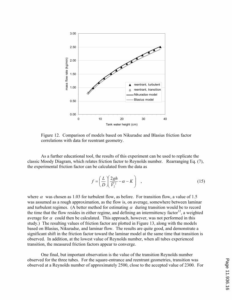
Figure 12. Comparison of models based on Nikuradse and Blasius friction factor

correlations with data for reentrant geometry.

As a further educational tool, the results of this experiment can be used to replicate the

classic Moody Diagram, which relates friction factor to Reynolds number. Rearranging Eq. (7),

the experimental friction factor can be calculated from the data as

ÕÕÖ

ÔÄÄÅ

Ã//Õ

ÖÔ

ÄÅÃ? K

V

gh

D

Lf c

2

2

2 , (15)

where c was chosen as 1.03 for turbulent flow, as before. For transition flow, a value of 1.5

was assumed as a rough approximation, as the flow is, on average, somewhere between laminar

and turbulent regimes. (A better method for estimating c during transition would be to record

the time that the flow resides in either regime, and defining an intermittency factor12

, a weighted

average for c could then be calculated. This approach, however, was not performed in this

study.) The resulting values of friction factor are plotted in Figure 13, along with the models

based on Blasius, Nikuradse, and laminar flow. The results are quite good, and demonstrate a

significant shift in the friction factor toward the laminar model at the same time that transition is

observed. In addition, at the lowest value of Reynolds number, when all tubes experienced

transition, the measured friction factors appear to converge.

One final, but important observation is the value of the transition Reynolds number

observed for the three tubes. For the square-entrance and reentrant geometries, transition was

observed at a Reynolds number of approximately 2500, close to the accepted value of 2300. For

Page 11.936.16

the rounded-entrance tube, however, transition occurred up to Re à 6000. This discrepancy is an

important result, because students often believe that the transition Reynolds number is a fixed

value. Of course, transition to turbulence can be delayed to even higher Reynolds numbers by

reducing the disturbances in the flow further.

The visual observation of transition and the measured transition Reynolds number

provide an opportunity for students to develop a physical concept of the Reynolds number and its

role in laminar and turbulent flows. The oscillating laminar and turbulent flow that occurs

during transition can be explained partly by the difference in wall friction between the two

regimes, and by the physical definition of the Reynolds number as the ratio of inertia forces to

viscous forces in the fluid. At the same water level, a laminar flow will produce more mass flow

than a turbulent flow, because the wall friction is lower in laminar flow. At higher flow

velocities, though, disturbances in the flow can overtake the viscous forces in the fluid to cause

turbulent flow. If the flow transitions to turbulent, however, the higher wall friction reduces the

velocity in the flow, and the flow can transition back to laminar as the viscous forces again

dominate.

What is confusing to many students is the apparent contradiction that in laminar flow,

viscous forces dominate, yet friction is reduced. This experiment provides an opportunity to

clarify that the Reynolds number pertains to inertia and viscous forces at a fluid particle level,

while the wall friction is a macroscale effect.

0.01

0.02

0.03

0.04

0.05

0.06

1000 2000 3000 4000 5000 6000 7000 8000 9000 10000

Reynolds number, Re

fric

tion f

acto

r, f

rounded

square

reentrant

Nikuradse model

Blasius model

Laminar flow model

Figure 13. Measured friction factor, and comparison to models of Nikuradse,

Blasius, and laminar flow. The empty symbols (ゴ,ﾖ,〉) refer to measurements

taken during transition.

Page 11.936.17

Pedagogical Approach

The pedagogy for this experiment is modeled after the work of Herb et al.13

, who applied

the Learning Cycle of Kolb14

and the 4MAT system of McCarthy15

to engineering instruction.

Specifically, the authors have adopted an approach to the experiment that can be described as

follows:

1. Modeling the System. The students are directed to examine the system, make appropriate

assumptions, and then develop a model to predict the mass flow rate of the water from

each of the exit tubes as a function of water height in the tank. This process is done with

a minimum of instructor input, for as open-ended an analysis as possible. However, the

students are directed to create two models for the system: a simplified model, neglecting

fluid friction, and an advanced model that includes friction effects. The purpose of the

simplified model is as a first, order-of-magnitude solution, as well as to examine the

relative effect of fluid friction by comparison with the advanced model. At the same

time, the students examine how the experiment will be operated and how the mass flow

rate will be measured (it is accomplished by weighing an amount of water collected in a

bucket over a measured period of time).

2. Predicting the Accuracy of the Model. The students are directed to perform uncertainty

analysis on the predicted and measured mass flow rate, and evaluate how accurate they

expect their results to be.

3. Testing the Model. The experiment is run, and data are collected. The data are used to

plot the mass flow rate of exiting water as a function of tank water height. In practice,

only four water heights are studied, which were carefully chosen so the resulting flow is

turbulent. Four data points is sufficient to demonstrate the efficacy of the models while

reducing the data collection to a reasonable level of effort.

4. Determining the Transition Reynolds Number. With the model for mass flow rate

successfully verified, the model can be used as a tool to “discover” the transition

Reynolds number. By shutting off the fill pump and allowing the tank to drain slowly,

students can observe when the turbulent flow first begins its transition from turbulent to

laminar flow. Because the water level is decreasing, the mass flow rate cannot be

measured with the “bucket-stopwatch” method. Instead, students record the water height

when transition begins, and use their model to calculate the average mass flow rate. (The

tank drains slowly enough that transient effects are negligible.) Thus, having developed a

model, they can now apply it to answer a new question.

Conclusions

The experiment developed in this work presents a simple problem to undergraduate fluid

mechanics students, which is to predict the mass flow rate of water exiting a constant-head tank.

The scenario, however, provides physical insight and promotes an engineering approach to

Page 11.936.18

experimentation that is not easily revealed in the classroom. Comparison of the model to the

experiment reveals several important effects:

‚ The model, an application of pipe flow theory, compares well to the mass flow rates

measured from the square-entrance and reentrant geometry tubes. The model slightly

under-predicts turbulent mass flow rate from the rounded-entrance tube. Observations

suggest that the difference might be attributed to the possibility of a laminar developing

length; however, the variation in empirical friction factor models was shown to be a

major factor as well.

‚ During transition, particularly for the rounded-entrance tube, the mass flow rate deviates

significantly from the turbulence-based pipe flow model. The mass flow rate is higher

than predicted, which is expected given that the transition flow actually alternates

between laminar and turbulent flow.

‚ The experiment was designed to result in transition flow at certain water tank heights.

Transition was marked by alternating laminar and turbulent flow, which is readily

observable. This feature allows students to test their understanding of the nature of the

Reynolds number and the structure of laminar and turbulent flows.

‚ The transition Reynolds number was approximately 2500 for the square-entrance and

reentrant tubes, close to the expected value of 2300. However, the rounded entrance tube

yielded a value of approximately 6000, demonstrating that by reducing disturbances, a

flow can attain higher velocities (and hence higher Reynolds numbers) before

transitioning to turbulence.

‚ Further analysis of the data gives measured values of friction factor, which, plotted

against Reynolds number, give a chart that closely matches the classic Moody Diagram.

Along with achieving the technical goals of the course, the pedagogy was developed to

reveal more than simply the verification of a pipe flow model. In particular,

‚ Performing uncertainty analysis reveals how accurate the model is expected to be prior to

running the experiment. The technique also allows for judging whether the differences

between a model and experimental data are “significant.”

‚ Students are asked not only to develop a model and verify it, but they are also directed to

use the model as a tool to discover something new – in this case, to measure the transition

Reynolds number. Furthermore, students discover that the transition Reynolds number is

not a fixed value, but rather an empirical one. This study is an excellent example of how

the Learning Cycle approach can be applied in the laboratory.

Acknowledgments

The authors wish to thank Professor Ernst Blattner and undergraduate student James

McDougall, who contributed to the development of this experiment. The authors also wish to

thank the Mechanical Engineering Student Fee Allocation Committee for financial support,

Edward L. “Tres” Clements III for assistance in fabrication of the apparatus, and J. Matthew

Patton for operational support and data collection.

Page 11.936.19

References

1. Bloom, B.S., Taxonomy of Educational Objectives, Allyn and Bacon, Boston, MA, 1984.

2. Allie, S., Buffler, A., Campbell, B., Lubben, F., Evangelinos, D., Psillos, D., and Valassiades, O., “Teaching

Measurement in the Introductory Physics Laboratory,” The Physics Teacher, Vol. 41, 23-30, 2003.

3. Deardorff, D.L., Introductory Physics Students’ Treatment of Measurement Uncertainty, Ph.D. Dissertation,

North Carolina State University, Raleigh, NC, 2001.

4. Reynolds, O., “An Experimental Investigation of the Circumstances Which Determine Whether the Motion of

Water Shall be Direct or Sinuous; And of the Law of Resistance in Parallel Channels,” Philosophical

Transactions of the Royal Society of London, Vol. 174, Pt. 3, 1883, pp. 935-982.

5. Fox, R.W. and McDonald, A.T., Introduction to Fluid Mechanics, 4th Ed., John Wiley and Sons, New York,

1992.

6. Coleman, H.W. and Steele, W.G., Experimentation and Uncertainty Analysis for Engineers, 2nd Ed., John

Wiley and Sons, New York, 1999.

7. Prandtl, L. and Tietjens, O.G., Applied Hydro-and Aeromechanics, Dover, New York, 1934.

8. Fowler, A.C. and Howell, P.D., “Intermittency in the Transition to Turbulence,” SIAM Journal of Applied

Mathematics, Vo. 63, No. 4, pp. 1184-1207, 2003.

9. Faisst, H. and Eckhardt, B., “Senstitive Dependence on Initial Conditions in Transition to Turbulence in Pipe

Flow,” Journal of Fluid Mechanics (submitted for publication).

10. White, F.M., Fluid Mechanics, 5th Ed., McGraw-Hill, 2003.

11. Benedict, R.P., Fundamentals of Pipe Flow, John Wiley and Sons, New York, 1980.

12. Schlichting, H., Boundary-Layer Theory, 7th Ed., McGraw-Hill, New York, 1979.

13. Harb, J.N., Durrant, S.O., and Terry, R.E., “Use of the Kolb Learning Cycle and the 4MAT System in

Engineering Education,” Journal of Engineering Education, 82, pp. 70-77, 1993.

14. Kolb, D.A., Experiential Learning: Experience as the Source of Learning and Development, Prentice-Hall,

Englewood Cliffs, NJ, 1984.

15. McCarthy, B., The 4MAT System: Teaching to Learning Styles with Right/Left Mode Techniques, EXCEL, Inc,

1987.

Page 11.936.20