Helsinki University of Technology Department of Signal Processing and Acoustics Espoo 2008 Report 1

MODELING OF NONLINEAR AND TIME-VARYING PHENOMENA IN THE GUITAR Jyri Pakarinen Dissertation for the degree of Doctor of Science in Technology to be presented with due permission for public examination and debate in Auditorium S4, Faculty of Electronics, Communications and Automation, Helsinki University of Technology, Espoo, Finland, on the 4th of March 2008, at 12 o'clock noon.

Helsinki University of Technology

Faculty of Electronics, Communications and Automation

Department of Signal Processing and Acoustics

Teknillinen korkeakoulu

Elektroniikan, tietoliikenteen ja automaation tiedekunta

Signaalinkäsittelyn ja akustiikan laitos

Helsinki University of Technology

Department of Signal Processing and Acoustics

P.O. Box 3000

FI-02015 TKK

Tel. +358 9 4511

Fax +358 9 460224

E-mail Lea.Soderman@tkk.fi

ISBN 978-951-22-9242-4 ISSN 1797-4267

Espoo, Finland 2008

ABABSTRACT OF DOCTORAL DISSERTATION HELSINKI UNIVERSITY OF TECHNOLOGY

P. O. BOX 1000, FI-02015 TKKhttp://www.tkk.fi

Author Jyri Pakarinen

Name of the dissertation

Manuscript submitted Sept. 29, 2007 Manuscript revised Jan. 9, 2008

Date of the defence March 4, 2008

Article dissertation (summary + original articles)MonographFacultyDepartment

Field of researchOpponent(s)Supervisor

Abstract

Keywords digital signal processing, musical acoustics, model-based sound synthesis, computer music

ISBN (printed) 978-951-22-9242-4

ISBN (pdf) 978-951-22-9243-1

Language English

ISSN (printed) ISSN 1797-4267

ISSN (pdf) ISSN 1797-4275

Number of pages 244

Publisher Helsinki University of Technology, Department of Signal Processing and Acoustics

Print distribution Report 1 / TKK, Department of Signal Processing and Acoustics

The dissertation can be read at http://lib.tkk.fi/Diss/

Modeling of Nonlinear and Time-Varying Phenomena in the Guitar

X

Faculty of Electronics, Communications, and AutomationDepartment of Signal Processing and AcousticsAudio Signal ProcessingProf. Julius O. Smith IIIProf. Vesa Välimäki

X

This dissertation studies some of the nonlinear and time-varying phenomena related to the guitar, and suggests newphysics-based models for their realistic discrete-time simulation for sound synthesis purposes. More specifically, thetension modulation phenomenon is studied and three new algorithms are introduced for synthesizing it. Energy-relatedproblems are discovered with conventional digital waveguide models when their pitch is varied, and two noveltechniques are suggested as a remedy. A new wave digital filter based real-time model is presented for simulating anonlinear vacuum-tube amplifier stage, found in typical high-quality guitar amplifiers. The first study of the handlingnoise on wound strings is presented. Using this information together with the time-varying digital waveguide energycompensation techniques mentioned above, a new real-time slide guitar synthesis algorithm is introduced. Also, thegeneration of flageolet tones on string instruments is discussed and a novel physics-based model for their simulation ispresented. In general, the results presented in this dissertation can be used for improving the current physics-basedstring instrument synthesizers and vacuum-tube amplifier models.

ABVÄITÖSKIRJAN TIIVISTELMÄ TEKNILLINEN KORKEAKOULU

PL 1000, 02015 TKKhttp://www.tkk.fi

Tekijä Jyri Pakarinen

Väitöskirjan nimi

Käsikirjoituksen päivämäärä 29.9.2007 Korjatun käsikirjoituksen päivämäärä 9.1.2008

Väitöstilaisuuden ajankohta 4.3.2008

Yhdistelmäväitöskirja (yhteenveto + erillisartikkelit)MonografiaTiedekuntaLaitosTutkimusalaVastaväittäjä(t)Työn valvoja

Tiivistelmä

Asiasanat digitaalinen signaalinkäsittely, musiikkiakustiikka, soitinmallinnus, tietokonemusiikki

ISBN (painettu) 978-951-22-9242-4

ISBN (pdf) 978-951-22-9243-1

Kieli Englanti

ISSN (painettu) ISSN 1797-4267

ISSN (pdf) ISSN 1797-4275

Sivumäärä 244

Julkaisija Teknillinen korkeakoulu, Signaalinkäsittelyn ja akustiikan laitos

Painetun väitöskirjan jakelu Raportti 1 / TKK:n Signaalinkäsittelyn ja akustiikan laitos

Luettavissa verkossa osoitteessa http://lib.tkk.fi/Diss/

Kitaran epälineaaristen ja aikamuuttuvien ilmiöiden mallinnus

X

Elektroniikan, tietoliikenteen ja automaation tiedekuntaSignaalinkäsittelyn ja akustiikan laitos

ÄänenkäsittelytekniikkaProf. Julius O. Smith IIIProf. Vesa Välimäki

X

Tämä väitöskirja käsittelee tiettyjä kitaraan liittyviä epälineaarisia ja aikamuuttuvia ilmiöitä, ja tarjoaa uusia, fysiikanlakeihin perustuvia, äänisynteesimalleja niiden todenmukaista simulointia varten. Kirjassa käsitellään kielenjännitysmodulaation aiheuttamaa epälineaarisuutta, ja ehdotetaan kolme uutta synteesialgoritmia sen mallinnukseen.Väitöskirjatyössä on havaittu soitinmallinnuksessa laajalti käytettyjen aaltojohtokielimallien vaimenemiseen liittyviäongelmia kielen äänenkorkeuden muuttuessa, ja kaksi kompensaatiomenetelmää ehdotetaan ratkaisuksi tähänongelmaan. Uusi aaltodigitaalisuodinpohjainen reaaliaikamalli esitetään kitaravahvistimissa yleisesti käytettyjenelektroniputkivahvistinasteiden simulointia varten. Kirjassa analysoidaan punottuja kieliä soitettaessa aiheutuviahälyääniä sekä esitellään tätä analyysia ja edellä mainittuja kompensaatiomenetelmiä käyttämällä aikaansaatuslidekitaran äänisynteesimalli. Kirjassa selitetään myös kielisoittimiin liittyvien huiluäänten syntymekanismi, sekätarjotaan uusi, kielen fysiikkaan pohjautuva algoritmi niiden syntetisoimiseksi. Tässä väitöskirjassa esitettyjä tuloksiavoidaan käyttää hyödyksi nykyisten soitin- ja vahvistinmallien toiminnan parantamisessa.

7

Preface

I consider myself a very lucky person. I have been given an opportunity to pursue two

of my greatest passions, music and science, and to combine them into my doctoral

work at the unit formerly known as Laboratory of Acoustics and Audio Signal Pro-

cessing at Helsinki University of Technology. For this opportunity, I am most grateful

to my supervisor and instructor, Prof. Vesa Välimäki. Vesa’s guidance, ideas, and

strive for efficiency have improved the quality of my thesis and helped me in getting

this work done in a relatively short time. I wish to express my gratitude to Prof. Matti

Karjalainen and Dr. Cumhur Erkut for support, inspiring discussions, and their endless

patience for explaining and re-explaining many physics-based modeling issues to me.

The contents of this thesis owe a lot to the co-writers of my publications: Dr. Stefan

Bilbao, Dr. Balázs Bank, Dr. Henri Penttinen, and Mr. Tapio Puputti. I want to thank

Mr. David Yeh for reading and commenting my manuscript, Mr. Luis Costa for his

careful proofreading, and my opponent Prof. Julius Smith for finding some time in

his busy schedule to travel from sunny California to not-so-sunny Finland for my doc-

toral defense. The effort of my pre-examiners, Prof. Federico Avanzini and Dr. Seppo

Uosukainen, both geniuses in their respective fields, is also acknowledged.

The acoustics lab is an extraordinary working environment, filled with interesting and

colourful personalities. Among the labsters, I especially want to thank our secretary

Lea Söderman for taking care of the bureaucracy and numerous practicalities involved

in my dissertation, my roommate Mairas for providing poor humor and five years worth

of intensive tech support, Mara and Hynde for other technical and computer-related is-

sues; Heidi-Maria Lehtonen, Laura Lehto, and Hannu Pulakka for second-lunch com-

pany; the Chechnyan rebels: Carlo Magi (In Memoriam 1980-2008), Toni Hirvonen,

ex-member Petri Korhonen, Ville Pulkki, Toomas Altosaar, and Miikka Tikander. I

am obliged to Prof. Gary Scavone, the Altosaar family, and all the great researchers at

8

McGill University, Montreal, for hosting my short-term scientific mission during the

fall of 2006.

I wish to acknowledge the financial supporters of this work: GETA graduate school, the

Graduate School of Electrical and Communications Engineering, Helsinki University

of Technology, Tekniikan edistämissäätiö, Nokia Foundation, Emil Aaltonen Founda-

tion, Academy of Finland (CAPSAS, project no. 104934), EU IST-2001-33059 project

(ALMA), and COST action no. 287 (ConGAS).

Also outside the lab, I feel privileged to be surrounded by such wonderful people. I

wish to thank my parents, grandparents, brother, and friends (you know who you are)

for supporting me. I greatly appreciate the rewarding counterbalance that our band

Superjaded (Pekkeri, Anna, Jesse, Janne, and Mikko) has provided for my life. Finally,

I wish to express my deepest gratitude and affection for my wife Annika and our lovely

daughter Mimosa, for their unconditional love and support.

Espoo, 12th of February 2008,

Jyri Pakarinen

9

Contents

Preface 7

Contents 9

List of Publications 11

Author’s Contribution 13

List of Abbreviations 17

List of Symbols 19

List of Figures 21

1 Introduction 23

1.1 History . . . . . . . . . . . . . . . . . . . . . . . . . . . . . . . . . 23

1.2 Nonlinearity and time-variance . . . . . . . . . . . . . . . . . . . . . 26

1.3 Aim and contents of this thesis . . . . . . . . . . . . . . . . . . . . . 28

2 Linear string acoustics 31

2.1 Ideal string vibration . . . . . . . . . . . . . . . . . . . . . . . . . . 31

2.2 Losses and stiffness . . . . . . . . . . . . . . . . . . . . . . . . . . . 35

3 Physics-based sound synthesis 38

3.1 Kirchhoff vs. wave models . . . . . . . . . . . . . . . . . . . . . . . 40

3.2 Digital waveguides . . . . . . . . . . . . . . . . . . . . . . . . . . . 41

3.3 Wave digital filters . . . . . . . . . . . . . . . . . . . . . . . . . . . 43

4 Modeling of nonlinear and time-varying phenomena 46

4.1 Geometric string nonlinearities . . . . . . . . . . . . . . . . . . . . . 46

10

4.1.1 Previous work . . . . . . . . . . . . . . . . . . . . . . . . . 46

4.1.2 Tension modulation . . . . . . . . . . . . . . . . . . . . . . . 47

4.1.3 Modeling of tension modulation . . . . . . . . . . . . . . . . 52

4.1.4 Energy compensation . . . . . . . . . . . . . . . . . . . . . . 53

4.2 Vacuum-tube nonlinearity . . . . . . . . . . . . . . . . . . . . . . . . 54

4.2.1 Operation of a triode stage . . . . . . . . . . . . . . . . . . . 55

4.2.2 Modeling of vacuum-tube amplifiers . . . . . . . . . . . . . . 58

4.3 Nonlinearities in other string instruments . . . . . . . . . . . . . . . . 61

4.4 Time-varying phenomena in guitars . . . . . . . . . . . . . . . . . . 62

4.4.1 Varying-length string . . . . . . . . . . . . . . . . . . . . . . 63

4.4.2 Fret noise . . . . . . . . . . . . . . . . . . . . . . . . . . . . 63

4.4.3 Time-varying spatial damping . . . . . . . . . . . . . . . . . 66

5 Conclusions and future development 68

References 72

Errata 95

11

List of Publications

This thesis consists of an overview and of the following publications which are referred

to in the text by their Roman numerals.

I J. Pakarinen, V. Välimäki, and M. Karjalainen, “Physics-based methods for

modeling nonlinear vibrating strings.” Acta Acustica united with Acustica,

No. 2, pp. 312-325, March/April, 2005.

II J. Pakarinen, M. Karjalainen, V. Välimäki, and S. Bilbao, “Energy behavior

in time-varying fractional delay filters for physical modeling of musical in-

struments.” In Proc. IEEE Intl. Conf. Acoust., Speech and Signal Proc., vol.

3, pp. 1-4, Philadelphia, PA, USA, March 19-23, 2005.

III V. Välimäki, J. Pakarinen, C. Erkut, and M. Karjalainen, “Discrete-time

modelling of musical instruments.” Reports on Progress in Physics, 69(1),

pp. 1-78, Jan. 2006.

IV M. Karjalainen and J. Pakarinen, “Wave digital simulation of a vacuum-tube

amplifier.” In Proc. IEEE Intl. Conf. Acoust., Speech and Signal Proc., vol.

5, Toulouse, France, May 14-19, 2006.

V J. Pakarinen, H. Penttinen, and B. Bank, “Analysis of the handling noises on

wound strings.” Journal of the Acoustical Society of America, 122(6), pp.

EL197-EL202, Dec. 2007.

VI J. Pakarinen, T. Puputti, and V. Välimäki, “Virtual slide guitar.” Accepted

for publication in Computer Music Journal, 2008.

VII J. Pakarinen, “Physical modeling of flageolet tones in string instruments.” In

Proc. 13th Eur. Signal Proc. Conf., Antalya, Turkey, September 4-8, 2005.

12

13

Author’s Contribution

Publication I: ”Physics-Based Methods for Modeling Nonlinear Vi-brating Strings”Previous digital waveguide models of tension modulated strings are lumped. This

means that physically correct interaction with the simulated string is possible only

at certain pre-defined locations. This article describes two novel spatially distributed

string models with tension modulation nonlinearity, which allow interaction at any spa-

tial location on the string. The author invented the novel finite difference algorithm,

coded both algorithms, and wrote the article.

Publication II: ”Energy Behavior in Time-Varying Fractional DelayFilters for Physical Modeling of Musical Instruments”This publication discusses the unnatural damping of digital waveguide strings with

time-varying length. Two novel algorithms are provided as a solution. The present

author formulated and implemented one of these methods, the controllable wave digital

filter delay line, and wrote Section 3, except for the second paragraph.

Publication III: ”Discrete-Time Modelling of Musical Instruments.”This study is an attempt to summarize all current musical instrument modeling tech-

niques into a thorough tutorial article. This is the first review article on the subject

that covers different modeling methods at such a detailed level. The author wrote Sec-

tions 8, 11, and most of Section 4. Also, a novel technique for simulating nonlinear,

energy-preserving strings in Sec. 11.2 was devised by the author.

Publication IV: ”Wave digital simulation of a vacuum-tube ampli-fier”In this article, a novel physical modeling technique for simulating vacuum-tube ampli-

14

fier stages is presented. Unlike most previous techniques, this method simulates each

circuit component in real time, resulting in a physically accurate but still real-time

computable model. The author wrote Sections 3.1 and 3.4, and collaborated in writing

Section 3.2. He also generated the related publication web page, and recorded the dry

demo samples.

Publication V: ”Analysis of the handling noises on wound strings.”The handling noise created by a moving finger on wound strings is studied. This is the

first scientific report analyzing this common phenomenon. The presented work enables

more realistic musical string synthesis in the future, since parametric models for the

handling noise can be generated. Research results reveal that the noise consists of time-

varying and static harmonic components. The former are due to the string windings,

while the latter are caused by the excitation of longitudinal string modes. The present

author is the main responsible for the underlying research. Discussions with co-authors

supported the planning of the work, and the measurements were carried out with co-

author #2. The author wrote the article, except for Sections IV and V.

Publication VI: ”Virtual Slide Guitar”A new physics-based model for synthesizing slide guitar sounds is presented. This

contains a new model for synthesizing the contact sounds between the slide tube and

the strings. The synthesis model operates in real-time and it is controlled using a

camera-based, gestural user interface. The author devised the model and wrote the

article, except for some parts of the introduction and of the section discussing the real-

time implementation. He also supervised the software implementation of the real-time

virtual slide guitar.

Publication VII: ”Physical modeling of flageolet tones in string in-struments”A new synthesis model for simulating flageolet tones on string instruments is pre-

15

sented. This method allows a more physical interaction with the string than the previ-

ous comb-filter-based techniques. For example, the amount of spatial damping can be

varied in time in a physically meaningful way. The present author is solely responsible

for the research and writing of this publication.

16

17

List of Abbreviations

3D Three-dimensional

BC Before Christ

DC Direct current

DSP Digital signal processing

DWG Digital waveguide

FIR Finite impulse response

IIR Infinite impulse response

K Kirchhoff

LTI Linear and time-invariant

MSW McIntyre, Schumacher, and Woodhouse (algorithm)

PDE Partial differential equation

W Wave

WDF Wave digital filter

18

19

List of Symbols

α [rad] Angle between the string and the soundboard at the termination

δ(·) Dirac’s delta function

κ [m] Radius of gyration

µ [kg/m] Linear mass density

τair [s] Time constant for decay caused by air damping

τint [s] Time constant for decay caused by internal string damping

τsup [s] Time constant for decay caused by energy loss through supports

τtot [s] Time constant for total decay

φn [rad] Initial phase of mode n

ct [m/s] Transversal wave propagation velocity

cl [m/s] Longitudinal wave propagation velocity

ds [m] Elongated length of a string segment

e Base for natural logarithms (e ≈ 2.7183)

f(x, t) [N/m] Excitation force density

fn [Hz] Frequency of mode n = 1, 2, 3 . . .

f0 [Hz] Fundamental frequency

n Mode index

t [s] Time variable

u [m] Transversal string displacement

u0 [m] Transversal string displacement at time t = 0

v [m] Longitudinal string displacement

w Torsional component of the string vibration

x, y, z [m] Spatial coordinates of a string segment

z−N Integer delay of length N

z−d Fractional delay of length d

(·)x Spatial derivative in the x-direction

20

(·)t Temporal derivative

A [m2] Cross-sectional area of a string

B Inharmonicity coefficient

Fn(t) [N] Excitation force of mode n

E [N/m2] Young’s modulus

Hn(t) Time-domain impulse response of mode n

Hl(z) Digital waveguide loss filter

Igk [A] Grid-to-cathode current of a vacuum-tube

Ipk [A] Plate-to-cathode current of a vacuum-tube

L [m] String length

L′ [m] Elongated string length

R(f) [1/s] Frictional resistance per unit mass

Rn [1/s] Frictional resistance per unit mass for mode n

T [N] String tension

T0 [N] Nominal string tension

Tu [N] Transversal component of string tension

Vg [V] Grid-to-ground voltage of a vacuum-tube

Vgk [V] Grid-to-cathode voltage of a vacuum-tube

Vk [V] Cathode-to-ground voltage of a vacuum-tube

Vp [V] Plate-to-ground voltage of a vacuum-tube

Vpk [V] Plate-to-cathode voltage of a vacuum-tube

21

List of Figures

3.1 A simple digital waveguide string . . . . . . . . . . . . . . . . . . . 42

3.2 The Kilroy bandstop circuit and its wave digital equivalent . . . . . . 44

4.1 Displaced string segment. . . . . . . . . . . . . . . . . . . . . . . . . 48

4.2 Typical string termination in a guitar. . . . . . . . . . . . . . . . . . . 51

4.3 Circuit diagram of a typical triode tube stage . . . . . . . . . . . . . . 56

4.4 Simulated characteristic plane of a typical triode tube (12AX7) . . . . 57

22

23

1 Introduction

1.1 History

Mankind has enjoyed the music of plucked string instruments for several millenia. The

earliest archeological illustrations of plucked string instruments have been found in the

Magdalenian cave in Ariége, France, where the rock art portrays a shaman holding an

object believed to be a musical bow, drawn approximately 17500 years ago [Sieveking,

1998]. Eventually, the primitive musical bow evolved into various plucked string in-

struments, such as harps, psalteries, and lutes. For an extensive tutorial on the history

of plucked instruments refer to [Jahnel, 1981]. One type of a gut-stringed lute, the 16th

century Spanish vihuela, can be seen as the ancestor of the modern six-string guitar.

The 19th century Spanish luthier Antonio de Torres (1817-1892) had a major impact

on the construction of the guitar by enlarging the body and introducing the fan-shaped

top-plate bracings [Fletcher and Rossing, 1988]. The concept of modern guitar was

dramatically changed with the introduction of the solid-body electric guitar by musical

instrument manufacturers Fender and Gibson in the 1950s.

First reported studies on vibrating strings were conducted by the Greek philosopher

Pythagoras (about 580-500 BC). He discovered that two plucked strings in equal ten-

sion produced pitches in consonant, or pleasing, intervals when their lengths were in

small integer ratios, such as 12, 1

3, 1

4, . . .. Pythagoras’ work was not continued until two

thousand years later, when an Italian luthist and composer Vincenzo Galilei (1520-

1591) found that contrary to the knowledge at that time, the string tension did not

follow the Pythagorean consonance ratios [Caleon and Subramaniam, 2007]. Instead,

he concluded that the tension ratio between two similar strings with equal lengths was

4:1 when they were tuned an octave apart [Foley, 2007].

24

Later, Vincenzo’s son, Galileo Galilei (1564-1642) revealed that the perceived pitch

of a vibrating string is determined by its frequency, i.e. the number of vibrations per

time unit [Caleon and Subramaniam, 2007]. Therefore, he correctly reasoned that the

pleasing consonance intervals were produced when the frequencies of the two strings,

rather than other string properties, were in integer ratios. At the same time, a French

philosopher and mathematician Marin Mersenne (1588-1648) discovered the relation

between a string’s length, tension, density, and the produced frequency [Foley, 2007].

The vibrational movement of an ideal string was studied in the early 18th century by

English mathematician Brook Taylor (1685-1731), who first noted in 1715 that the ac-

celeration of the string was proportional to its curvature [Mumford, 2006]. Using the

theory of calculus, introduced by Sir Isaac Newton (1643-1727) and Gottfried Wil-

helm Leibnitz (1646-1716) in the late 17th century, Daniel Bernoulli (1700-1782) was

able to derive the partial differential equation for an ideal string. He also provided a

solution in 1738 using separation of variables, which was later refined by Leonhard

Euler (1707-1783) and Joseph Louis Lagrange (1736-1813) [Robinson, 1982].

In 1747 a new solution to the wave equation was presented by the French mathemati-

cian Jean le Rond d’Alembert (1717-1783). He stated [Lindsay, 1973] that the solution

can be seen as a superposition of two arbitrary wave components, traveling in opposite

directions on the string. After this, Bernoulli, Euler, Lagrange, and d’Alembert de-

bated over the true general solution for the wave equation for several years [Shenitzer,

1998]. In 1759, starting from a finite set of linearly connected elementary masses, La-

grange showed that the harmonic vibration of a string is obtained as the number of the

elements approaches infinity [Rayleigh, 1945]. The discussion was finally concluded

in 1807, when the French mathematician and physicist Jean Baptiste Joseph Fourier

(1768-1830) showed that any function, e.g. the initial displacement of a string, can be

given as an infite sum of sinusoids.

25

As musicians have known for long, the vibrating string has to be connected to an

instrument body for sufficient sound radiation. Thus, the vibrational properties of the

musical instrument itself have a major impact on the produced sound. There are many

studies on the vibration of a guitar body in the literature (e.g. [Fletcher and Rossing,

1988], see [Richardson, 2003] for an overview), but since it is essentially a linear and

time-invariant phenomenon1, it will not be discussed further in this thesis. For electric

guitars, the magnetic pickup and amplifier properties also contribute a great deal to the

sound. Electric guitar body vibrations have been studied in [Esposito, 2003], and a

report on magnetic pickups can be found in [Jungmann, 1994]. The effect of a guitar

amplifier will be discussed in Chapter 4.2.

The birth of computers in the mid-twentieth century gave new, powerful tools for musi-

cal instrument research. The first discrete-time string models were presented by Hiller

and Ruiz in the early 1970s [Hiller and Ruiz, 1971a,b]. Article III provides a more

thorough discussion on the simulation of a vibrating string. Several discrete-time gui-

tar body models have been presented during the last two decades, starting from simple

filters [Karjalainen and Laine, 1991; Karjalainen et al., 1991, 1993b], to more sophisti-

cated admittance-based [Cuzzucoli and Lombardo, 1999; Woodhouse, 2004] and finite

element [Elejabarrieta et al., 2001; Derveaux et al., 2003; Bader, 2003, 2005; Bécache

et al., 2005] models. Hybrid body models containing warped filters, resonators, and

reverb algorithms have been presented in [Karjalainen et al., 1999; Penttinen et al.,

2000, 2001b]. A comparison between synthesized and measured guitar tones has been

published in [Woodhouse, 2004].

1An opposing view has been presented in [Besnainou et al., 2001], but it is generally consideredinvalid [Erkut, 2002; Penttinen, 2006].

26

1.2 Nonlinearity and time-variance

The definition of nonlinearity is probably best made through negation. A system with

input x and output f(x) is considered linear, if it is both

• additive, i.e. if f(x1 + x2) = f(x1) + f(x2) and

• homogeneous, i.e. if f(αx) = αf(x), for all α.

An intuitive way of illustrating linearity is to plot the output of a system as a function

of the input. For memoryless linear systems, the result is always a straight line through

the origin, hence the term linear. On the other hand, if a system fails to fulfill either of

the requirements above, it is nonlinear. The input-output relation of a nonlinear system

is a curve, which is not a straight line.

A system is considered time-variant, if its response properties depend explicitly on

time. In other words, an input signal x(t) produces the output

• y(t) = f(x(t), t) at a given time instant t.

Thus, due to the time-variance, the system output can change even if x(t) remains con-

stant. In conclusion, nonlinearity and time-variance are two distinct properties. Thus, a

system might be either nonlinear or time-variant, both, or neither. Systems, which are

linear and do not depend explicitly on time are called linear and time-invariant (LTI)

systems.

So, what is the practical relevance of whether a system is LTI or non-LTI, one might

ask. The answer is that for LTI systems, a special set of analysis tools, called LTI

27

system theory, can be used. Probably the most fundamental property of an LTI system

is that its behavior is explicitly defined by its impulse response. The impulse response

is, as its name implies, the output of the system when a single impulse is given as

the input. When the impulse response of a lumped, i.e. dimensionless, LTI system

is known, its response for any input signal can be obtained by convolving the input

signal in the time domain with the impulse response. This is a remarkable simplifica-

tion since it reduces all the functionality of the system into one signal. For spatially

distributed systems, convolving the impulse response in the space domain with an ar-

bitrary excitation gives meaningful results only if the system is space invariant, as in

the hypothetical case of an infinitely long string, for example. Since real strings are

not space invariant, simple spatial convolution does not suffice. This will be discussed

further in Sec. 2.

For non-LTI systems, this reduction is not possible. The impulse response of a non-

linear system tells only how the system reacts to an impulse input, but in general it

does not tell anything about the system’s response to any other signal. Therefore, if

the behavior of a nonlinear system is to be defined only by its input-output relation

(the so-called black-box approach), one would have to measure the system’s output

for every imaginable input signal. For time-varying systems, the case is even more

complicated, since the response for a given input depends also on when the input was

fed to the system.

Obviously, LTI systems are a lot easier to analyze or simulate than non-LTI systems

from the engineering point of view. Thus, it is not surprising that various systems are

often considered LTI, although, in the strict sense, they are not. In many cases, the

parameter ranges are chosen so that the inaccuracy due to this erroneous assumption

is negligible, i.e. the system is nearly-enough LTI. However, as nature does not follow

simple mathematical restrictions, the LTI assumption does not hold for real systems in

general. Especially in the case of musical instruments, there are various phenomena in

28

which the LTI assumption does not yield realistic results.

1.3 Aim and contents of this thesis

The scope of this thesis is physics-based sound synthesis of string instruments. The

purpose of this branch of research is to use the laws of physics to artificially create

the sounds of real sounding objects, such as musical instruments. These synthesis

techniques can then be implemented for example in electronic keyboards, computer

programs, and mobile devices. Traditionally, most plucked string instruments have

been considered LTI in the synthesis point of view. Although usually faster to com-

pute, LTI string instrument models often sound too artificial or static to be interesting

for a human listener. The present thesis aims to address this problem by adding the

effect of many important non-LTI properties involved in real string instruments, gui-

tars in particular. The inclusion of these phenomena results in more realistic sound

synthesizers that respond to the user’s action more intuitively than previous synthesis

models.

In addition to the physical accuracy of these methods, their ability to produce real-time

sound synthesis is of paramount importance. Usually, there is a trade-off between these

requirements, so a choice has to be made between physical accuracy and system sim-

plicity. Since the author’s main motive for physical modeling of musical instruments

is real-time sound synthesis, the choice of generating models which are sufficiently

accurate for human listeners but can still produce synthesized sound in real time has

been made.

This thesis consists of a summary and seven articles. The articles are published in inter-

national peer-reviewed journals and conferences, and the summary aims to give a con-

29

cise description of the results obtained as well as to provide more thorough background

information. The summary consists of five sections. Section 1 discusses the history of

string instrument research, introduces the concept of nonlinearity and time-variance,

and clarifies the aim and purpose of this work. Section 2 studies the vibrational behav-

ior of a linear string, and section 3 gives a brief overview of the simulation methods

used in this thesis. Section 4 discusses the guitar-related nonlinear and time-varying

phenomena that are studied and modeled in articles I-VII. Section 5 gives a conclusion

of the scientific results presented in this thesis. The rest of the thesis consists of the

articles.

Articles I and III introduce new spatially distributed sound synthesis algorithms for

tension modulated strings. These models simulate the initial pitch descent and mode

coupling effects of real string instruments. Unlike previous nonlinear string models,

the new algorithms allow the user to correctly interact with the string at any location

along its length, thus increasing the flexibility of string synthesizers.

Article II presents two new methods for compensating for artificial energy losses en-

countered in current varying-pitch string models. Using the presented techniques, more

realistic models for strings with rapidly varying pitch can be generated. The nonlinear

string model introduced in article III, and the virtual slide guitar introduced in article

VI use these methods.

Article IV introduces a new model for real-time simulation of a guitar tube ampli-

fier stage. In contrast to most previous algorithms, this technique allows a realistic

component-level simulation of the amplifier circuit. More importantly, the proposed

model is modular, which means that the circuit topology can be easily varied. This

simulation scheme is a first step towards a new type of a virtual guitar amplifier, where

the user could easily alter the device’s component values and circuit connections and

immediately hear the resulting change in amplifier’s tone. This future guitar ampli-

30

fier simulator could also be used a prototyping tool for conventional tube amplifier

designers.

Handling noises on wound strings is analyzed in article V, which is the first scientific

study of this nonlinear and time-varying phenomenon to the author’s best knowledge.

These squeaky contact sounds are created by a moving finger on a wound string, and

they can frequently be heard in most guitar recordings, even though musicians often try

to avoid creating them. The inclusion of these effects is crucially important if realistic

guitar synthesis is desired, since a total lack of handling sounds make a synthetic string

instrument sound too machine-like and dull. Using the results presented in article V,

more realistic synthesis algorithms for wound string instruments can be generated.

Article VI introduces a new musical instrument, the virtual slide guitar. The physics-

based synthesis engine of this instrument uses the research results presented in articles

II and V, and it is capable of creating realistic slide guitar sounds. The virtual slide

guitar has a gestural camera-based user interface, so that the user can play this virtual

instrument simply by making slide guitar playing movements in front of a camera,

similarly as presented in Karjalainen et al. [2006].

Finally, a physics-based synthesis model for flageolet tones on string instruments is

presented in article VII. Flageolet tones (a.k.a. harmonics) can be generated nearly

with all string instruments by damping the string at some specific locations. The ad-

vantage of the proposed technique over previous flageolet tone modeling mechanisms

is that it allows a more realistic simulation also when the damping is varying in time,

which often happens in real playing situations.

31

2 Linear string acoustics

2.1 Ideal string vibration

The vibration of a string can be decomposed into four orthogonal components. This

means that each infinitely short string segment can move in four independent direc-

tions, called polarizations. The first two polarizations, horizontal and vertical, are

transversal to the string, i.e. they move perpendicular to the direction of the string. The

third polarization, longitudinal, expresses the compressional waves within the string

medium. Finally, the fourth polarization, torsional, describes the string’s movement

around its longitudinal axis.

Although the torsional polarization plays an important role in characterizing the vibra-

tion of a bowed string, it has a negligible effect in the case of plucked strings. Thus,

only transversal and longitudinal vibrations are discussed in what follows. Also, since

the physical laws dictating the behavior of the horizontal and vertical polarizations are

the same, mainly the transverse string displacement u is discussed in what follows.

The mathematics in the remainder of this section follow the derivations presented in

several textbooks, e.g. [Fletcher and Rossing, 1988], except that here the focus is on

obtaining the string’s impulse response.

Consider an ideal string – a perfectly flexible, lossless cord – which is tightly fixed

at both ends. The transversal vibration of this theoretical string is governed by the

linearized inhomogeneous wave equation

utt − c2tuxx =

f(x, t)

µ, (2.1)

where ut and ux denote the temporal and spatial partial derivatives, respectively. Vari-

32

able

ct =

√T

µ(2.2)

denotes the transversal wave velocity, where T is the tension of the string and µ is

its linear mass density, i.e. mass per unit length. Variable f in Eq. (2.1) denotes an

external excitation force density, which depends on the longitudinal coordinate x and

time, t. In other words, Eq. (2.1) relates the string’s acceleration to its curvature and

an external excitation. The longitudinal vibration of the string obeys a similar rule as

in Eq. (2.1), except that for the longitudinal wave velocity

cl =

√EA

µ, (2.3)

where E is Young’s modulus and A is the cross-sectional area of the string.

As discussed in Sec. 1.1, d’Alembert solved Eq. (2.1) using the traveling-wave solu-

tion

u(x, t) = u0(x + ctt) + u0(x− ctt), (2.4)

where u0(x) = 12u(x, 0) denotes the initial string displacement. Although the synthesis

algorithms discussed later in this thesis are mainly based on d’Alembert’s solution, it

is educational to take a closer look at the closed-form solution of Eq. (2.1), presented

by Bernoulli:

u(x, t) =∞∑

n=1

sin(nπx

L

)[an cos

(nπctt

L

)+ bn sin

(nπctt

L

)]. (2.5)

Here, L is the length of the string, so that 0 ≤ x ≤ L. Symbols an and bn are constants

defining the modal amplitudes. By setting t = 0 in Eq. (2.5), the initial displacement

of the string can be given as

u(x, 0) =∞∑

n=1

an sin(nπx

L

). (2.6)

For the initial velocity, taking the time derivative of Eq. (2.5) and setting t = 0 yields

ut(x, 0) =∞∑

n=1

nπct

Lbn sin

(nπx

L

). (2.7)

33

In order to solve an, Euler and Lagrange suggested multiplying each side of Eq. (2.6)

by sin(kπx/L) and integrating from 0 to L [Robinson, 1982] to get2

an =2

L

∫ L

0

u(x, 0) sin(nπx

L

)dx. (2.8)

Similarly, Eq. (2.7) gives

bn =2

nπct

∫ L

0

ut(x, 0) sin(nπx

L

)dx. (2.9)

In other words, if the initial string displacement and velocity are known, the vibration

of an ideal string is explicitly given by Eqs. (2.5), (2.8), and (2.9). It must be noted

that Eqs. (2.5) through (2.9) give the solution for the homogeneous wave equation,

corresponding to the case where f(x, t) = 0 in Eq. (2.1).

Since the ideal string is an LTI system, the closed-form solution to the inhomogeneous

wave equation can be obtained by using the impulse response. This would mean setting

f(x, t) = δ(x − x0)δ(t) in Eq. (2.1), i.e. using a (spatial and temporal) force density

impulse as an excitation. If the initial string displacement is zero, applying a force

impulse at x = x0 at time t = 0 corresponds to setting the initial acceleration to

utt =δ(x− x0)δ(t)

µ, (2.10)

due to Newton’s second law. Hence, the initial velocity becomes

ut =

∫δ(x− x0)δ(t)

µdt =

δ(x− x0)

µ. (2.11)

Substituting Eq. (2.11) into (2.9) and reformulating Eq. (2.5) (note that for zero initial

displacement an = 0) gives

u(x, t) =∞∑

n=1

sin(nπx

L

) 2

nπct

∫ L

0

δ(x− x0)

µsin(nπx

L

)dx sin

(nπctt

L

). (2.12)

2More rigorously, it can be stated that the functions√

2L sin

(nπxL

)are an orthonormal system of the

space L(2)[0, L].

34

Additionally, noting that since the frequency of mode n is fn = nct/(2L), the transver-

sal wave velocity can be written as ct = 2Lfn/n. Also, since it is easy to see that the

integral in Eq. (2.12) equals sin (nπx0/L) /µ, the string vibration resulting from the

force impulse becomes

u(x, t) =1

πLµ

∞∑n=1

sin(nπx

L

) 1

fn

sin (2πfnt) sin(nπx0

L

). (2.13)

Thus, Eq. (2.13) represents the impulse response of an ideal string, fixed at both ends.

In order to get the response for any point-like excitation f(x0, t), time-domain convo-

lution must be applied.

For obtaining the string response to any spatially distributed excitation f(x, t), the case

is different. It must be noted that although the system under discussion is LTI, it is not

spatially invariant. This means that the vibration of a point on the string depends on

its longitudinal coordinate, and simply convolving f(x, t) with Eq. (2.13) in space

does not yield the correct solution. Instead, one must spatially integrate f(x, t) with

the modal shapes in order to get the temporal excitation for each mode separately. In

other words, since Eq. (2.13) gives the string response for any point-like excitation,

the string response for a spatially distributed excitation can be obtained using superpo-

sition, i.e. summing over the spatial points. Formally, the string response for arbitrary

force excitation is thus given as

u(x, t) =1

πLµ

∞∑n=1

sin(nπx

L

)Hn(t) ∗ Fn(t), (2.14)

where ∗ denotes convolution and

Hn(t) =1

fn

sin (2πfnt) (2.15)

is the impulse response of mode n and

Fn(t) =

∫ L

0

sin(nπx

L

)f(x, t)dx (2.16)

is the excitation force of that mode.

35

2.2 Losses and stiffness

In contrast to the ideal string, real strings lose their energy and their vibration grad-

ually decays. Three main reasons for the decay are [Fletcher and Rossing, 1988] air

damping, internal damping, and transfer of mechanical energy through the supports.

The first two of these are dissipative mechanisms due to viscoelastic and thermody-

namic losses. They convert the kinetic energy of the string into heat and are therefore

irreversible processes. Mechanical energy transfer is a process in which the kinetic

energy flows from the string to the instrument body. A small portion of this energy can

also flow back to the string, thus making the energy transfer bidirectional in nature.

These loss types are briefly discussed in what follows. For a more detailed study of

loss mechanisms in musical strings, refer to [Valette, 1995].

Air damping is caused by the viscous flow that retards the movement of the string.

There is also a small energy transfer from the string directly into the surrounding air,

but since the string itself is a poor radiator (its diameter is small compared to the wave-

length) this loss is often considered negligible. For a given frequency, air damping

causes an exponential decay of vibration. This decay is expressed using the time con-

stant τair, which is a function of the properties of the string and air and the vibration

frequency [Fletcher and Rossing, 1988]. A physical interpretation for τair is the time it

takes for the string vibration to decay to 1/e part due to air damping only.

Internal damping consists of all thermo-3 and viscoelastic forces that resist movement

within the string structure. The decay caused by internal damping is characterized

with time constant τint, which has a similar physical interpretation as τair, except that

instead of air damping, only internal damping is considered. String stiffness introduces

additional hysteretic damping, which can also be included in τint, if the frequency-

3Although thermoelastic losses generally play a minor role in metallic strings, they can have a no-ticeable effect in a certain frequency region, as stated in [Zener, 1937; Valette, 1995].

36

dependent behavior of the internal losses are suitably selected. For wound strings,

dry friction, i.e. the friction between contiguous turns of the wound wire, also damps

the string movement. The detailed effect of this phenomenon is, however, not well

understood [Valette, 1995].

Damping through the end supports is often characterized by the coupling impedance,

or its reciprocal, admittance (mobility), between the string and the instrument body.

The impedance gives the ratio between force and the resulting velocity, and it depends

on the string and body properties, contact type, and vibration frequency. The damping

effect of the end supports is again of exponential type and thus it can be given as a

time constant τsup, which essentially is a function of impedance [Fletcher and Rossing,

1988].

The net effect of the major losses can now be expressed using a resistance term [Morse,

1948; Bank, 2006]

R(f) =1

τtot

=1

τair

+1

τint

+1

τsup

, (2.17)

which is the effective frictional resistance per unit mass. Naturally, R depends not

only on the vibration frequency, but also on the physical properties of the string and air

discussed above. In practice, the correct value of R cannot be defined analytically, but

must be measured from the decay times of real string instruments over some frequency

range. For this reason, it is most practical to denote R as a function of frequency only.

As opposed to ideal strings, real strings are not perfectly flexible, but possess some

bending stiffness. This means that in addition to the string tension T , there is another

restoring force that tends to keep the string in its equilibrium position. In practice,

the stiffness causes dispersion, i.e. harmonic frequencies become stretched so that the

upper partials end up higher in frequency when compared to the perfectly harmonic

case. Stiffness plays a major role in the vibration of thick strings, such as those used

37

in the piano, but it is not important for guitar strings due to their smaller diameter

[Järveläinen and Karjalainen, 2006].

Finally, the partial differential equation (PDE) governing the motion of a lossy string

with nonzero stiffness is given as

utt − c2tuxx + 2R(f)ut +

EAκ2

µuxxxx = f(x, t), (2.18)

where κ is the radius of gyration. The solution to Eq. (2.18) is the same as that given

in Eq. (2.14), except that the losses cause the mode impulse response presented in Eq.

(2.15) to have an additional multiplicative decay term [Morse, 1948]:

Hn,lossy(t) =e−Rnt

fn

sin (2πfnt) , (2.19)

where Rn is the frictional resistance for mode n. In principle, a finite damping through

the supports lowers the modal frequencies since the vibrational length of the string

increases. However, if the damping is small, this shift in frequencies can be considered

negligible, i.e.

fn =1

2π

[(πnct

l

)2

−R(f)2

] 12

≈ nct

2l. (2.20)

The stiffness causes the spreading of the modal frequencies so that

fn = f0n√

1 + Bn2, (2.21)

where f0 is the fundamental frequency and

B =EA

T

(πκ

L

)2

(2.22)

is called the inharmonicity coefficient [Fletcher et al., 1962].

38

3 Physics-based sound synthesis

The purpose of physics-based sound synthesis is to create artificial instrument sounds

using the laws of physics. In most cases, it is desirable that the synthesized sounds re-

semble the sound of real instruments as much as possible. In some cases, however, the

synthesized sounds should represent the tones played on an imaginary instrument, a

musical tool for which a real-life implementation would be impractical or even impos-

sible to build (consider, e.g. the 24-string virtual super guitar, introduced in [Laurson

et al., 2002]).

At the time of the writing of this thesis, the largest drawback of physics-based sound

synthesis is the poor sound quality compared to sample-based synthesis methods. This

is caused by the fact that in order to be able to run in real-time, the physical models

often have to be simplified greatly. Also, insufficient control data causes the models

to sound unrealistic; high-quality guitar synthesis, for example, is hard to implement

with a different user interface than the one in a real guitar. Sample-based synthesis

methods can obviously produce very realistic instrument sounds, but they are greatly

limited in flexibility, since they are essentially just modified record-and-playback ma-

chines. Although sample-based approach is suitable for synthesizing instruments with

a relatively small expressive range, such as the organ, it fails to reproduce the nuances

of a more expressive instrument, such as the violin. An excellent article on evaluation

of different sound synthesis techniques can be found in [Jaffe, 1995].

The major advantage in all model-based sound synthesis is the flexibility; the same

model can produce a myriad of different sounds. For example, a general bowed-string

instrument model could produce all the tones of the whole bowed-string instrument

family. Preferably, the synthesizer would conceptually act like a real instrument, so

that the user’s action would produce an intuitive change in the produced sound. This

39

way, a musician could play the virtual model just like a real instrument, without first

having to undergo special training for getting used to the model parameters. It must be

noted that such a system does not necessarily have to be implemented using physics;

sample-based synthesizers and spectral synthesis models can aim to do this as well,

although it usually is much more complicated.

Here lies, however, probably the greatest advantage of physics-based sound synthesis:

the mapping between the model parameters and the aspects of the resulting sound is

objective, i.e. defined by the universal laws of nature. In other synthesis methods, this

mapping is subjective. This means that in non-physics-based synthesis techniques the

system designer gets to choose the representation of the model parameters. Thus, he

might call a certain parameter “distance” just because changing that parameter seems

to change the distance between the listener and the virtual instrument in his own opin-

ion. In physics-based models, mother nature has made these decisions already, and

there is no need for the error-prone subjective part. It must be noted that in practice, it

is advisable to use also perceptual information in deciding which physical phenomena

are to be simulated and to which extent. If real-time sound synthesis is to be obtained,

there is little use of simulating processes that do not yield audible results. Perceptual

studies of synthesized string instrument sounds have been reported e.g. in [Järveläinen,

2003].

An exhaustive tutorial on physics-based sound synthesis methods is provided in article

III. For this reason, only those two modeling techniques, digital waveguides (DWGs)

and wave digital filters (WDFs), that are essential for understanding the research results

presented in this thesis are discussed in sections 3.2 and 3.3, respectively. Furthermore,

the discussion is focused on guitar-related modeling, although these paradigms can be

used for simulating various other systems as well. Both digital waveguides and wave

digital filters are based on the wave-formalism, which is elaborated in the following.

40

3.1 Kirchhoff vs. wave models

As discussed in article III, physics-based sound synthesis techniques can be divided

into two categories: those that operate with Kirchhoff (K for short) variables, and

those that operate with wave (W) variables. Operating with K variables means that in

addition to the system states, also the digital signals inside the model represent phys-

ical quantities directly. Often these quantities are arranged in pairs (called Kirchhoff

pairs, hence the name) such as voltage and current or pressure and volume flow. The

operation of a system is then usually defined using immittances, i.e. impedances or

admittances, which give the relation between the Kirchhoff pair.

Operating with W variables means that instead of using physical quantities directly, the

model uses d’Alembert’s approach (see Sec. 2) and represents its variables as wave de-

compositions of the physical quantities. Thus, in a W-based model, the signals inside

the synthesis engine represent waves, e.g. pressure waves, traveling in opposite direc-

tions, and the actual physical quantities are obtained by summing the waves together.

In W-based models, the operation of a system is defined by its reflectance instead of

its immittance. Reflectance is defined as the relation between the wave going into the

system and the wave coming out (i.e., reflecting) from the system. From the signal

processing point of view the system reflectance can be seen as equivalent to the sys-

tem’s transfer function, representing the ratio between the input and output signals in

the frequency domain.

A major conceptual difference between K- and W-models is that in W-based systems

the direction of causality is fixed, as discussed in article III. In other words, a decision

has been made that the input causes the output. In K-models, the direction of causality

is left open. For example, in a mass-spring oscillator one might think that the restoring

force of the spring causes the mass to gain velocity, or alternatively that the velocity of

41

the mass results in spring displacement and therefore causes a restoring force. If the

system is LTI, the direction of causality is not important from the modeling point of

view, since both interpretations yield the same model. However, with non-LTI systems

a different interpretation leads to a different model. W-based modeling techniques

avoid this ambiguity by forcing the system designer to choose explicitly the input and

output variables.

It must be noted that although immittances and reflectances are frequency-domain

quantities, the actual modeling is most often carried out in the time domain. In practice,

this is obtained by approximating them with digital filters.

3.2 Digital waveguides

The term digital waveguide modeling was introduced by Julius Smith in the 1980s

[Smith, 1985, 1987]. The same principle of using wave variables and scattering junc-

tions had been used already earlier in the Kelly-Lochbaum speech synthesis model

[Kelly and Lochbaum, 1962; Strube, 2000]. Also the Karplus-Strong string model

[Karplus and Strong, 1983] can be seen as a simplified case of a DWG system, although

its relation to physics-based modeling was not apparent at the time of its introduction.

For an excellent tutorial on DWG modeling, see [Smith, 1992].

In practice, DWG systems can be efficiently constructed using delay lines which con-

tain the traveling wave components. In DWG strings, the time delay of the delay loop

equals the inverse of the string’s fundamental frequency. For correct tuning, fractional

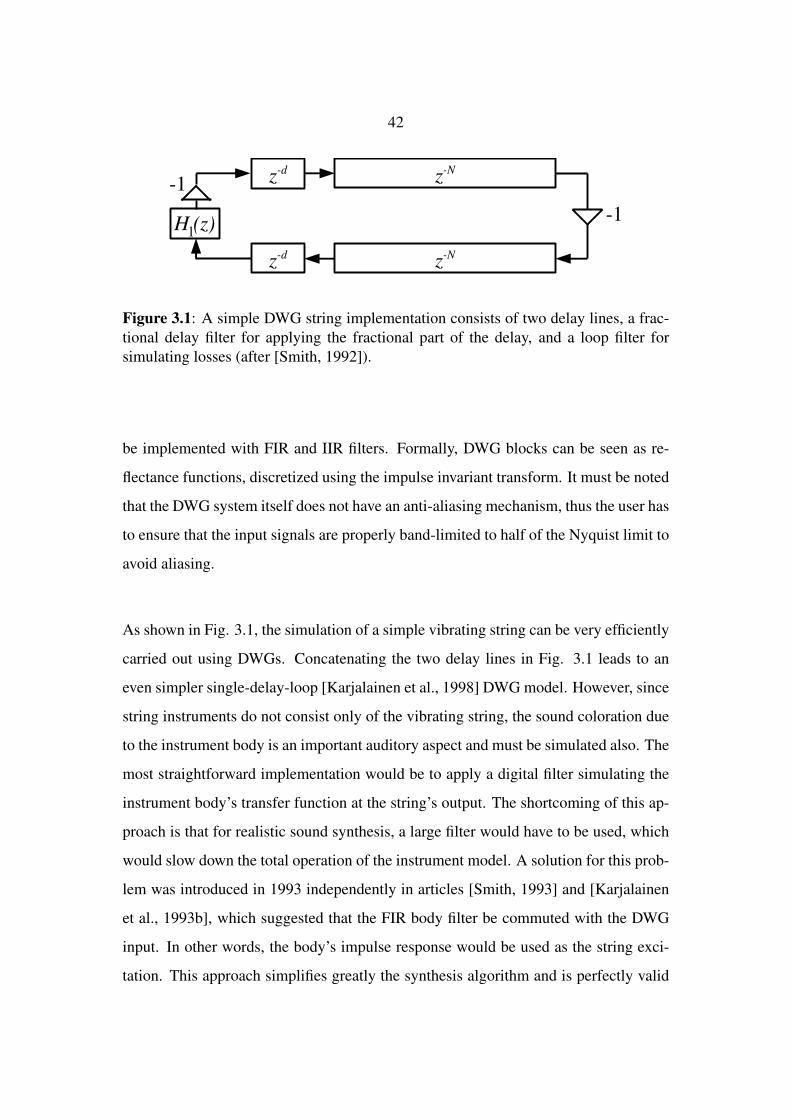
delay filters [Laakso et al., 1996] are used. Figure 3.1 illustrates a simple DWG string.

In the most straightforward implementation, only a pointer update per time step is re-

quired for modeling wave propagation. Simulation of losses, inharmonicities, etc. can

42

Figure 3.1: A simple DWG string implementation consists of two delay lines, a frac-tional delay filter for applying the fractional part of the delay, and a loop filter forsimulating losses (after [Smith, 1992]).

be implemented with FIR and IIR filters. Formally, DWG blocks can be seen as re-

flectance functions, discretized using the impulse invariant transform. It must be noted

that the DWG system itself does not have an anti-aliasing mechanism, thus the user has

to ensure that the input signals are properly band-limited to half of the Nyquist limit to

avoid aliasing.

As shown in Fig. 3.1, the simulation of a simple vibrating string can be very efficiently

carried out using DWGs. Concatenating the two delay lines in Fig. 3.1 leads to an

even simpler single-delay-loop [Karjalainen et al., 1998] DWG model. However, since

string instruments do not consist only of the vibrating string, the sound coloration due

to the instrument body is an important auditory aspect and must be simulated also. The

most straightforward implementation would be to apply a digital filter simulating the

instrument body’s transfer function at the string’s output. The shortcoming of this ap-

proach is that for realistic sound synthesis, a large filter would have to be used, which

would slow down the total operation of the instrument model. A solution for this prob-

lem was introduced in 1993 independently in articles [Smith, 1993] and [Karjalainen

et al., 1993b], which suggested that the FIR body filter be commuted with the DWG

input. In other words, the body’s impulse response would be used as the string exci-

tation. This approach simplifies greatly the synthesis algorithm and is perfectly valid

43

as long as the string can be considered LTI. For nonlinear or time-varying strings, e.g.

strings that change their pitch during vibration, commuted DWG synthesis cannot di-

rectly be used, since changing the total delay length would vary the instrument body

resonances.

3.3 Wave digital filters

Wave digital filters are a special class of digital filters with physically meaningful pa-

rameters. The WDF technique was formulated by Alfred Fettweis in the late 1960s

[Fettweis, 1971] for discrete-time modeling of analog electric circuits. For a tutorial

on WDF modeling, see [Fettweis, 1986]. Unlike DWGs, WDFs are designed for sim-

ulating lumped, i.e. point-like, systems, although they can be extended for simulating

multidimensional systems in some cases [Bilbao, 2001].

Another difference between DWGs and WDFs is the type of discretization: WDFs

discretize the system reflectance using the bilinear transform, which maps the analog

frequency axis in the s-domain inside the unit circle in the z-domain. This avoids

aliasing of the system response, but introduces warping of the high frequencies since

the infinite analog frequency is mapped onto the Nyquist frequency in the digital do-

main. It must be noted that this warping takes place only in the system response and

not in the wave variables themselves. Thus, also with WDFs, the input signal must be

band-limited to half of the Nyquist limit to avoid signal aliasing. In practice, DWG

and WDF systems can be interconnected (through a scaling coefficient in some cases),

as the wave variables are essentially the same. Wave digital filters are especially well-

suited for modeling electric circuits. This is convenient for simulating the electric

guitar, since the circuitry involved in the magnetic pickups and the amplifier forms an

essential part of the instrument’s sound.

44

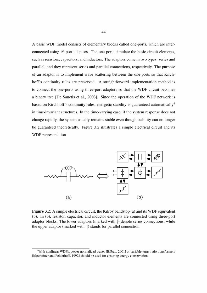
A basic WDF model consists of elementary blocks called one-ports, which are inter-

connected using N -port adaptors. The one-ports simulate the basic circuit elements,

such as resistors, capacitors, and inductors. The adaptors come in two types: series and

parallel, and they represent series and parallel connections, respectively. The purpose

of an adaptor is to implement wave scattering between the one-ports so that Kirch-

hoff’s continuity rules are preserved. A straightforward implementation method is

to connect the one-ports using three-port adaptors so that the WDF circuit becomes

a binary tree [De Sanctis et al., 2003]. Since the operation of the WDF network is

based on Kirchhoff’s continuity rules, energetic stability is guaranteed automatically4

in time-invariant structures. In the time-varying case, if the system response does not

change rapidly, the system usually remains stable even though stability can no longer

be guaranteed theoretically. Figure 3.2 illustrates a simple electrical circuit and its

WDF representation.

Figure 3.2: A simple electrical circuit, the Kilroy bandstop (a) and its WDF equivalent(b). In (b), resistor, capacitor, and inductor elements are connected using three-portadaptor blocks. The lower adaptors (marked with ◦|) denote series connections, whilethe upper adaptor (marked with ||) stands for parallel connection.

4With nonlinear WDFs, power-normalized waves [Bilbao, 2001] or variable turns-ratio transformers[Meerkötter and Felderhoff, 1992] should be used for ensuring energy conservation.

45

Each port in a WDF network holds a computational parameter, the port impedance,

which is used in calculating the wave scattering. Effectively, the port impedance values

of all circuit elements are interdependent. By choosing the individual port impedances

correctly, the one-port elements become extremely simple DSP blocks, where the in-

stantaneous dependency between input and output is removed. For a list of some typ-

ical circuit components and their WDF realizations, see article III, p. 41. Since the

signal flow between each element is bidirectional, special scheduling is needed in or-

der for the WDF network to be realizable. The binary-tree approach [De Sanctis et al.,

2003] uses reflection-free ports for implementing the scheduling. A detailed descrip-

tion of the binary-tree method is provided in Sec. 8 of article III.

If the modeled circuit is LTI, the port impedances remain constant throughout the sim-

ulation. Unfortunately, this is not the case with nonlinear WDF elements. Consider,

for example, that the leftmost resistor in Fig. 3.2(a) would be nonlinear. This would

mean that its resistance value, and thus the port impedance, would vary as a function

of the incoming signal. Since the port impedances are interconnected through adaptor

elements, changing the port impedance of any element would require a recalculation

of every port impedance within the circuit. The binary-tree approach [De Sanctis et al.,

2003] can handle one nonlinear element in the WDF network using its special schedul-

ing technique. Other nonlinearities can be connected through delay blocks, if desired.

For memoryless nonlinearities, i.e. nonlinear resistors, the reflectance can be imple-

mented as a simple lookup table, as done in article IV. For nonlinearities with memory

(nonlinear reactances), special mutator elements can be used [Sarti and De Poli, 1999].

It must be noted that, with nonlinearities, aliasing cannot always be avoided even with

properly bandlimited input signals. The reason for this is that the nonlinear distortion

creates high-frequency signal components that will alias back to the baseband. This

aliasing is audible if the nonlinearity is too strong. In article IV, aliased components

are suppressed by using temporal oversampling.

46

4 Modeling of nonlinear and time-varying

phenomena

This chapter focuses on explaining a set of non-LTI phenomena related to the guitar,

namely tension modulation, vacuum-tube nonlinearity, time-varying pitch and damp-

ing, and handling noise. Previous simulation attempts are recapitulated, and new

synthesis models introduced in articles I-IV and VI-VII are discussed. For a gen-

eral overview of musical instrument nonlinearities, see [Fletcher, 1998]. Modeling of

various non-LTI effects in musical instruments are discussed in article III and [Bilbao,

2007].

4.1 Geometric string nonlinearities

The term “nonlinear strings”, widely used in the literature, usually refers to a special

vibrational aspect, where the spatial structure of the string causes nonlinear behavior.

Thus, the nonlinearity is caused by the geometry of the string rather than its material

properties, for example. This type of nonlinearity will be studied more thoroughly in

what follows.

4.1.1 Previous work

Many publications considering geometric string nonlinearities can be found in the lit-

erature; see overviews in [Narasimha, 1968; Tolonen, 2000; Erkut, 2002; Bank, 2006].

First studied by Kirchhoff in the late 19th century and later revised by Carrier [Carrier,

1945], the geometric nonlinearities in strings are responsible for various phenomena.

47

One of the most audible effects is the initial pitch glide phenomenon [Carrier, 1945;

Valette, 1995], where a heavily plucked string experiences a pitch descent as its vibra-

tion decays due to tension modulation. Another interesting effect is the generation of

missing modes due to nonlinear coupling, where new vibrational modes are generated

after the plucking event [Miles, 1965; Legge and Fletcher, 1984; Feng, 1995; Valette,

1995; Conklin, 1999]. Transversal polarizations are also coupled due to the nonlinear-

ity, causing the vibration to have a whirling motion [Murthy and Ramakrishna, 1964;

Miles, 1965; Anand, 1969; Elliott, 1980; Gough, 1984; Miles, 1984]. The coupling

between transversal and longitudinal modes [Morse and Ingard, 1968; Giordano and

Korty, 1996] in turn leads to generation of another set of harmonics [Nakamura and

Naganuma, 1993], called phantom partials [Conklin, 1999]. The generation mecha-

nism of phantom partials is explained in detail in [Bank and Sujbert, 2005].

In thin strings with relatively high tension, such as those used in a guitar, the longitudi-

nal and transverse vibrations can be considered separable [Oplinger, 1960; Narasimha,

1968; Anand, 1969], as will be discussed later in this thesis. Coupling between the

transverse modes through torsional vibration has been discussed in [Watzky, 1992].

The nonlinearity also causes the string to experience amplitude jumps under forced

oscillation [Murthy and Ramakrishna, 1964; Tufillaro, 1989; Hanson et al., 1994]. An

excellent classification of geometric string nonlinearities can be found in [Bank, 2006].

4.1.2 Tension modulation

A more thorough explanation for the pitch glide and generation of missing harmonics

due to tension modulation is given in the following. The derivation follows the one

presented in [Legge and Fletcher, 1984]. A similar approach has also been used in

[Bank, 2006].

48

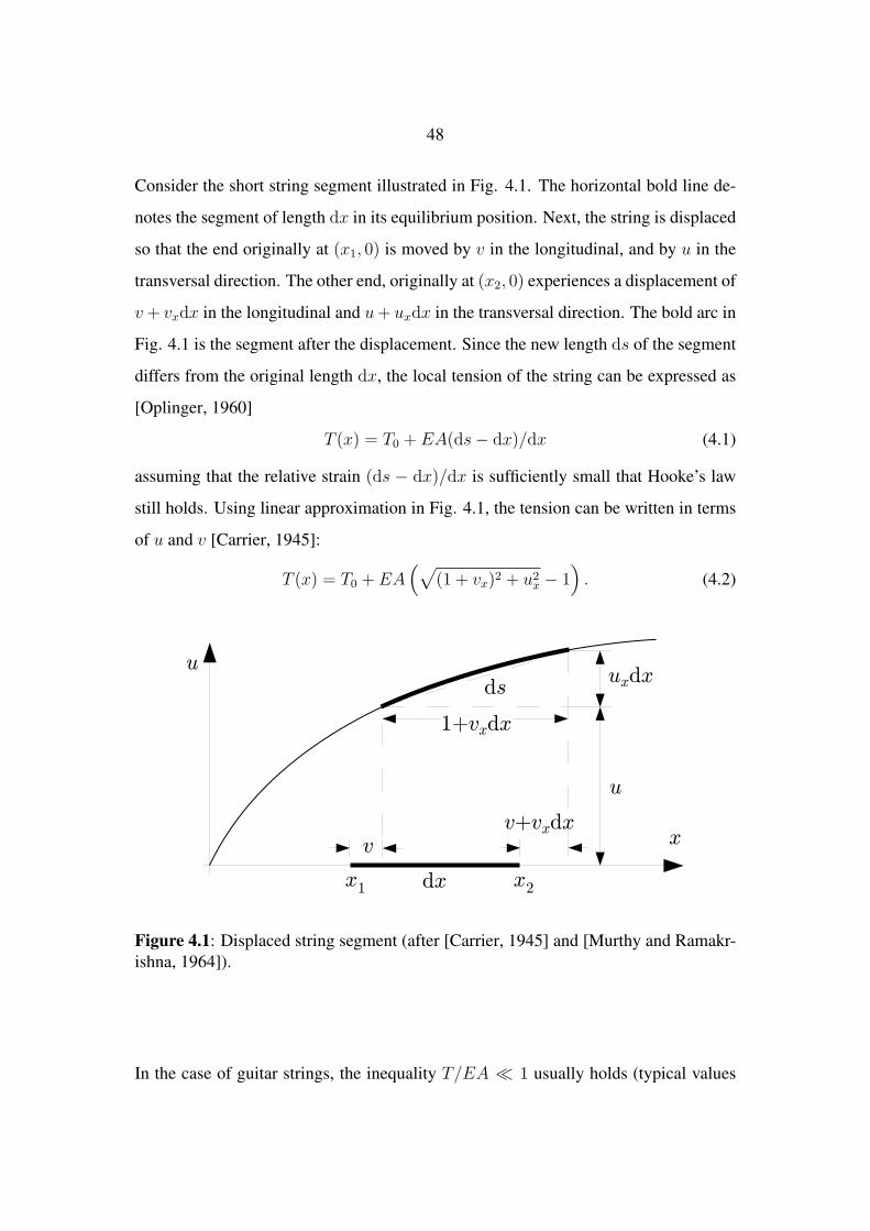
Consider the short string segment illustrated in Fig. 4.1. The horizontal bold line de-

notes the segment of length dx in its equilibrium position. Next, the string is displaced

so that the end originally at (x1, 0) is moved by v in the longitudinal, and by u in the

transversal direction. The other end, originally at (x2, 0) experiences a displacement of

v + vxdx in the longitudinal and u + uxdx in the transversal direction. The bold arc in

Fig. 4.1 is the segment after the displacement. Since the new length ds of the segment

differs from the original length dx, the local tension of the string can be expressed as

[Oplinger, 1960]

T (x) = T0 + EA(ds− dx)/dx (4.1)

assuming that the relative strain (ds − dx)/dx is sufficiently small that Hooke’s law

still holds. Using linear approximation in Fig. 4.1, the tension can be written in terms

of u and v [Carrier, 1945]:

T (x) = T0 + EA(√

(1 + vx)2 + u2x − 1

). (4.2)

Figure 4.1: Displaced string segment (after [Carrier, 1945] and [Murthy and Ramakr-ishna, 1964]).

In the case of guitar strings, the inequality T/EA � 1 usually holds (typical values

49

for a low-e string made of steel are T ≈ 76N , E ≈ 20× 1010 Nm2 , and A ≈ 1.04mm2).

Thus, looking at Eqs. (2.2) and (2.3) it can be seen that the longitudinal wave velocity

is considerably larger than the transversal one. A simplifying assumption can now be

made; if the longitudinal tension propagation is considered instantaneous5, each point

on the string will experience the same tension at a given time instant, and the tension

becomes uniform [Oplinger, 1960]6:

T = T0 + EA(L′ − L)/L, (4.3)

where

L′ =

∫ L

0

√1 + u2

xdx ≈ L +1

2

∫ L

0

u2xdx (4.4)

is the elongated length, i.e. the total length of the displaced string. Substituting Eq.

(4.4) in Eq. (4.3) gives an approximation for the spatially uniform tension

T = T0 +1

2

EA

L

∫ L

0

u2xdx. (4.5)

In the lossy case, the impulse response of the string can be written using Eqs. (2.14)

and (2.19) as

u(x, t) =∞∑

n=1

an sin(nπx

L

)sin(2πfnt + φn)e−Rnt, (4.6)

where

an =1

πLµfn

. (4.7)

The φn term in Eq. (4.6) simply denotes the initial phase of mode n. Substituting Eq.

(4.6) into Eq. (4.5) yields the time-varying tension as a function of the string vibration:

T (t) = T0 +1

2

EA

L

∫ L

0

(∞∑

n=1

annπ

Lcos(nπx

L

)sin(2πfnt + φn)e−Rnt

)2

dx. (4.8)

5More precisely, the excitation bandwidth must be small enough so that the longitudinal modes areexcited well below their resonances [Bank, 2006].

6This simplification is sometimes referred to as Anand’s argument due to a more detailed three-dimensional study presented in [Anand, 1969]. However, it first appears in [Oplinger, 1960].

50

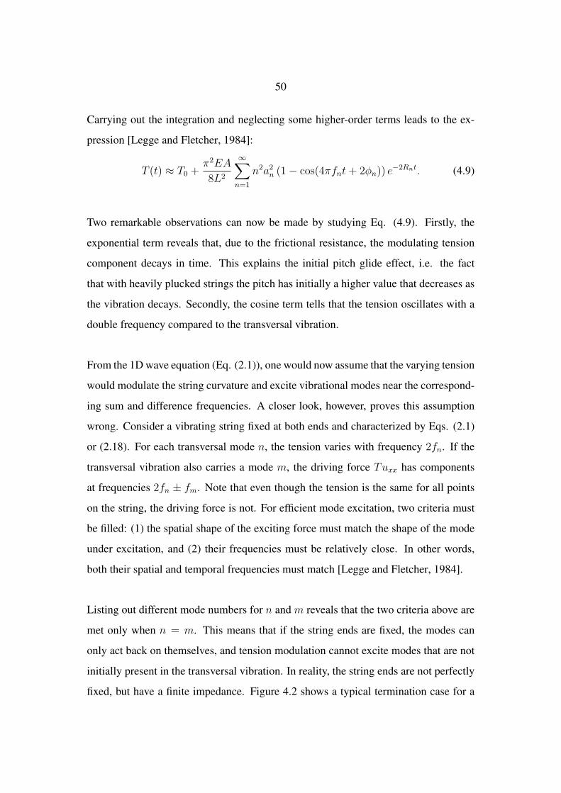
Carrying out the integration and neglecting some higher-order terms leads to the ex-

pression [Legge and Fletcher, 1984]:

T (t) ≈ T0 +π2EA

8L2

∞∑n=1

n2a2n (1− cos(4πfnt + 2φn)) e−2Rnt. (4.9)

Two remarkable observations can now be made by studying Eq. (4.9). Firstly, the

exponential term reveals that, due to the frictional resistance, the modulating tension

component decays in time. This explains the initial pitch glide effect, i.e. the fact

that with heavily plucked strings the pitch has initially a higher value that decreases as

the vibration decays. Secondly, the cosine term tells that the tension oscillates with a

double frequency compared to the transversal vibration.

From the 1D wave equation (Eq. (2.1)), one would now assume that the varying tension

would modulate the string curvature and excite vibrational modes near the correspond-

ing sum and difference frequencies. A closer look, however, proves this assumption

wrong. Consider a vibrating string fixed at both ends and characterized by Eqs. (2.1)

or (2.18). For each transversal mode n, the tension varies with frequency 2fn. If the

transversal vibration also carries a mode m, the driving force Tuxx has components

at frequencies 2fn ± fm. Note that even though the tension is the same for all points

on the string, the driving force is not. For efficient mode excitation, two criteria must

be filled: (1) the spatial shape of the exciting force must match the shape of the mode

under excitation, and (2) their frequencies must be relatively close. In other words,

both their spatial and temporal frequencies must match [Legge and Fletcher, 1984].

Listing out different mode numbers for n and m reveals that the two criteria above are

met only when n = m. This means that if the string ends are fixed, the modes can

only act back on themselves, and tension modulation cannot excite modes that are not

initially present in the transversal vibration. In reality, the string ends are not perfectly

fixed, but have a finite impedance. Figure 4.2 shows a typical termination case for a

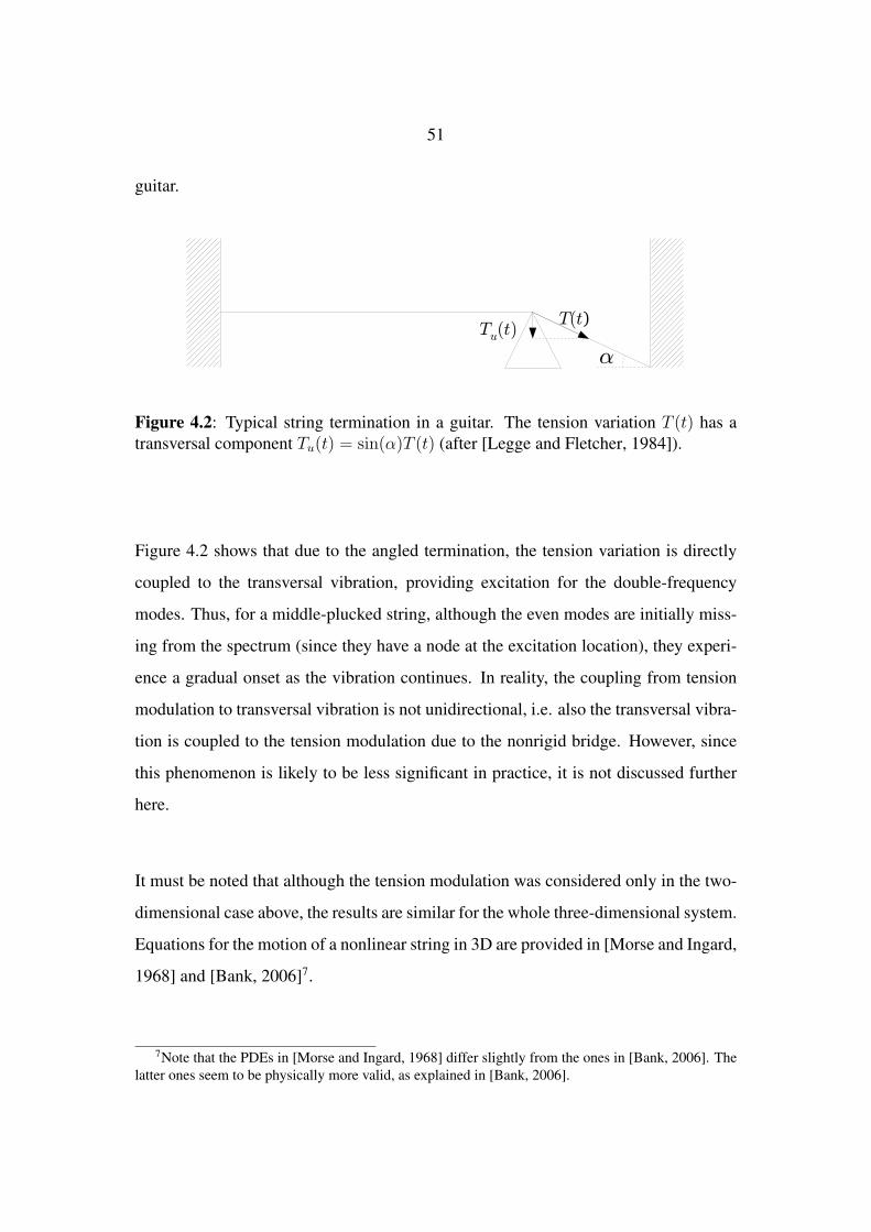
51

guitar.

Figure 4.2: Typical string termination in a guitar. The tension variation T (t) has atransversal component Tu(t) = sin(α)T (t) (after [Legge and Fletcher, 1984]).

Figure 4.2 shows that due to the angled termination, the tension variation is directly

coupled to the transversal vibration, providing excitation for the double-frequency

modes. Thus, for a middle-plucked string, although the even modes are initially miss-

ing from the spectrum (since they have a node at the excitation location), they experi-

ence a gradual onset as the vibration continues. In reality, the coupling from tension

modulation to transversal vibration is not unidirectional, i.e. also the transversal vibra-

tion is coupled to the tension modulation due to the nonrigid bridge. However, since

this phenomenon is likely to be less significant in practice, it is not discussed further

here.

It must be noted that although the tension modulation was considered only in the two-

dimensional case above, the results are similar for the whole three-dimensional system.

Equations for the motion of a nonlinear string in 3D are provided in [Morse and Ingard,

1968] and [Bank, 2006]7.

7Note that the PDEs in [Morse and Ingard, 1968] differ slightly from the ones in [Bank, 2006]. Thelatter ones seem to be physically more valid, as explained in [Bank, 2006].

52

4.1.3 Modeling of tension modulation

Numerical simulation of the tension modulation nonlinearity has been carried out by

several techniques. Energy-preserving finite-difference models have been introduced

in [Furihata, 2001; Bilbao, 2004a,b] (see an overview in [Bilbao, 2005]). The advan-

tage of these models is that their numerical stability can be guaranteed. On the other

hand, their computational requirements are often too demanding for real-time sound

synthesis. A modal-based approach for nonlinear string simulation has been taken in

[Trautmann and Rabenstein, 2000] and [Bilbao, 2004b]. Also, hybrid models using

finite-difference strings with resonators for simulating longitudinal modes have been

presented [Bank and Sujbert, 2004; Bank, 2006], as well as models which use separate

DWGs for simulating different polarizations [Bank and Sujbert, 2003]. Stabilization

issues related to undamped nonlinear strings have been addressed in [Shahruz, 1999;

Kobayashi and Sakamoto, 2007].

One popular modeling method has been to use DWGs, where the length of the de-

lay line has been varied in order to simulate the initial pitch glide phenomenon [Kar-

jalainen et al., 1993a; Välimäki et al., 1998; Välimäki et al., 1999; Tolonen et al.,

1999, 2000; Erkut et al., 2002]. A similar approach had been taken already earlier

by Pierce and Van Duyne for modeling a vibrating string terminated in a nonlinear

spring [Pierce and Van Duyne, 1997]. However, since these algorithms use a lumped

fractional delay at the termination of the waveguide, the whole string essentially be-

comes a dimensionless black-box model, where physically meaningful interaction is

restricted to the string ends only. Article I tackles this deficiency by presenting a spa-

tially distributed nonlinear digital waveguide string model, which allows interaction

with the entire length of the string. This new waveguide model uses time-varying

first-order allpass filters evenly distributed along the string. The desired delay change

is evaluated from the tension variation, and the allpass filter coefficients are updated

53

each time sample. It must be noted that although the model is presented in a spatially

distributed form, the string tension is considered uniform.

Article I also introduces an experimental finite-difference model of a spatially dis-

tributed nonlinear string. The nonlinearity is simulated by using fractional delay filters

to estimate the string state between sampling instants and thus varying the temporal

sampling interval during run-time. Although the digital waveguide model discussed

above performs better than the finite difference one, the derivation of the latter nicely

shows that tension modulation can be simulated in a finite difference scheme by simply

varying the time step of the algorithm during run-time.

4.1.4 Energy compensation

Another shortcoming of the previous nonlinear DWG models (and time-varying waveg-

uides in general), is the fact that changing the waveguide length at run time introduces

artificial energy variation. Consider, for example, a DWG string which is rapidly short-

ened to half of its original length. If no precautions are taken, half of the signal samples

in the delay lines are discarded, and the string loses its energy. It must be noted that

even though the energetic behavior of a real string under pitch change has not been

clarified, this type of artificial energy loss caused by the delay-line structure of the

DWG is clearly not physical and must be compensated for.

Article II presents two novel energy-compensation methods to resolve this problem.

The first method uses the string length variation to evaluate the artificial energy change

each time sample, and adjusts a scaling parameter inside the waveguide accordingly.

The second method uses power-normalized WDF one-ports in series connection as

delay lines in a DWG string. Due to the energy-preserving properties of power-

normalized WDF elements, the resulting varying-tension DWG does not encounter

54

the artificial energy change. Using the power-normalized DWG string presented in II,

a new energy-preserving nonlinear DWG string model is proposed in article III. Basi-

cally, this nonlinear DWG model can be seen as an extension of the spatially distributed

DWG string in article I, with inclusion of the WDF energy-conservation technique de-

scribed in article II. The energy-scaling method, also introduced in II, is used in the

virtual slide guitar, presented in article VI.

4.2 Vacuum-tube nonlinearity

Probably the single most important nonlinear phenomenon related to the electric gui-

tar is the distortion effect caused by nonlinear amplification, vacuum-tube amplifiers

in particular. From the engineering point of view, vacuum-tube technology seems out-

dated in comparison to the modern solid-state (i.e. transistor-based) technology, due

to the large size, high power consumption, poor durability, and expensive price of the

tube elements. Therefore, it might be surprising that throughout the history of the elec-

tric guitar, vacuum-tube amplifiers have been favored by most professional guitarists.

A major reason for this is that the distinctive tone of tube amplifiers was popularized

in the 1950s and 60s by the early rock’n roll bands. At that time, before the transistor

revolution, vacuum-tube technology was the only viable solution for electric audio am-

plification. Since then, the perceptually favorable warm distortion of tube amplifiers

has become the de-facto standard of the rock’n roll guitar sound. From the auditory

point of view, vacuum tubes and transistors behave very similarly when operated in

their linear range. However, major audible differences emerge when the signal starts

to saturate [Hamm, 1973], as happens nearly always with the electric guitar.

A typical guitar amplifier unit consists of a preamplifier, equalization circuit, and a

power amplifier. The purpose of the preamplifier is to magnify the relatively weak

55

signal from the magnetic guitar pickups and to provide buffering so that the pickup

response is not changed by the amplifier circuitry. The equalization unit (a.k.a. tone-

stack) provides a typical V-shaped equalization for compensating the pickup’s high

resonance at mid-frequencies, and gives the user additional control over the tone. The

power amplifier boosts the signal so that it is strong enough to drive a loudspeaker.

In the so-called all-tube guitar amplifiers, both the pre- and power amplifier circuits

are implemented with tube technology. Typically, they consist of one or more tube

stages, i.e. circuits that contain a vacuum-tube and other electric components. The

power amplifier also contains an output transformer for generating a suitable voltage

for the loudspeaker and often a phase-splitter circuit for feeding two equal but opposite

signals to the power tubes.

The nonlinear behavior of a triode tube-stage, encountered in preamps, is studied fur-

ther in the following. The same principles can be applied for tetrode and pentode stages

found in power amplifiers, although their operational details are different. An overview

of vacuum-tubes used in audio applications can be found in [Barbour, 1998], while

a more detailed tutorial on different vacuum-tube circuits is provided in [Langford-

Smith, 1954]. The detailed vacuum-tube physics is discussed in [Spangenberg, 1948].

4.2.1 Operation of a triode stage

The circuit diagram of a typical triode tube stage is shown in Fig. 4.3, where the oval

symbol denotes the triode tube. Physically, the tube consists of three electrodes: plate,

cathode, and grid, thus the name triode. The electrodes are marked with black dots in

Fig. 4.3, and the symbols Vp, Vk, and Vg denote the voltages between these respective

points and the ground. The electrodes are enclosed in a glass shell, and a vacuum is

generated inside this casing. The operational idea of the triode tube is that the current

flowing from the plate to the cathode is controlled by the grid, which is located in

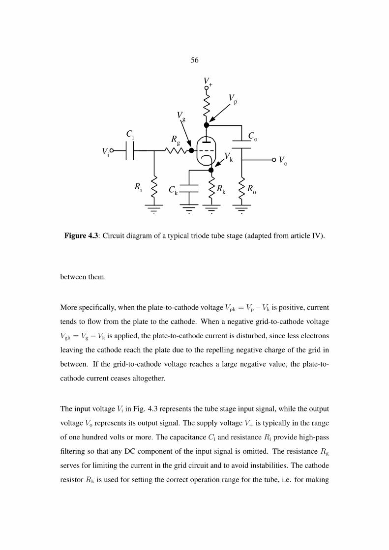
56

Figure 4.3: Circuit diagram of a typical triode tube stage (adapted from article IV).

between them.

More specifically, when the plate-to-cathode voltage Vpk = Vp−Vk is positive, current

tends to flow from the plate to the cathode. When a negative grid-to-cathode voltage

Vgk = Vg − Vk is applied, the plate-to-cathode current is disturbed, since less electrons

leaving the cathode reach the plate due to the repelling negative charge of the grid in

between. If the grid-to-cathode voltage reaches a large negative value, the plate-to-

cathode current ceases altogether.

The input voltage Vi in Fig. 4.3 represents the tube stage input signal, while the output

voltage Vo represents its output signal. The supply voltage V+ is typically in the range

of one hundred volts or more. The capacitance Ci and resistance Ri provide high-pass

filtering so that any DC component of the input signal is omitted. The resistance Rg

serves for limiting the current in the grid circuit and to avoid instabilities. The cathode

resistor Rk is used for setting the correct operation range for the tube, i.e. for making

57

a negative bias for Vgk. The cathode capacitance Ck bypasses the cathode resistor,

increasing gain at audio frequencies. The output capacitance Co and resistance Ro

separate the DC component from the plate voltage Vp and yield the output voltage Vo.

The plate-to-cathode current Ipk (which causes the output voltage Vo) is a nonlinear

function of the plate-to-cathode and grid-to-cathode voltages:

Ipk = f(Vpk, Vgk). (4.10)

Figure 4.4 illustrates the function in Eq. (4.10) for a typical triode tube 12AX7. It

must be noted that besides being nonlinear, this relation also is essentially implicit,

since Vpk depends on Ipk. If a high-amplitude signal is fed to the input of the tube

Figure 4.4: A simulated characteristic plane of a typical triode tube (12AX7). Thecurrent Ipk is a nonlinear function of both the plate-to-cathode and grid-to-cathodevoltages Vpk and Vgk.

stage, it might happen that the grid-to-cathode voltage becomes positive. In this case,

58

a current Igk starts to flow from the grid to the cathode, thus producing a voltage drop

IgkRg across Rg. This reduces the grid voltage and causes an additional nonlinearity.

4.2.2 Modeling of vacuum-tube amplifiers

Despite their acclaimed tone, tube amplifiers have some impractical properties: they

are heavy, expensive, and relatively fragile. On the other hand, different classes of

tube amplifiers are known to have quite different tonal qualities. Thus, for obtaining a

variety of high-quality tones, guitarists have traditionally had to resort to an expensive

arsenal of different tube amplifiers. For these reasons, there has been a demand for

modeling amplifiers in recent decades. Several companies (e.g. Roland, Line6, Vox,

Fender, Yamaha) have pursued making products that realistically simulate a collection

of tube amplifiers.

Although solid-state amplifiers also produce nonlinear distortion, it is essentially dif-

ferent from the vacuum-tube distortion (see, e.g. [Santo, 1994]). Thus, for realistic

solid-state modeling of tube amplifiers, special transistor-based emulation circuits have

been suggested: [Todokoro, 1976; Sondermeyer, 1981, 1984; Pritchard, 1989, 1991;

Butler, 1991; Tiers and Kieffer, 1991; Pritchard, 1992, 1995; Sondermeyer, 1996;

Pritchard, 1997, 1998a,b,c]. Also, transistor-based models for simulating the guitar

amplifier’s loudspeaker [Pittman and Buck, 1990], and the loudspeaker-microphone-

setup [Kelsey, 1998] have been reported.

Since the 1990s, the trend of tube amplifier modeling has shifted towards simulation

via digital signal processing (DSP). The advantage of digital algorithms over analog

electric circuits is their versatility: new model parameters are simply loaded into the

system memory when the user switches between amplifier models. Also, the whole

virtual amplifier can be implemented as a computer program, and model updates can

59

be made available through the Internet. The term virtual analog modeling describes

this general approach for digitally simulating analog electric circuits. Some digital

amplifier modeling patents can be found in the literature [Kuroki and Ito, 1998; Doidic

et al., 1998; Suruga et al., 2002; Gustafsson et al., 2004] while some others incorporate

also the simulation of special audio effects [Pennock et al., 2003], and multi-channel

amplifier modeling [Limacher et al., 2005, 2006]. Tube amplifiers and other nonlinear

signal processing systems can also be approximated by varying the coefficients of a

linear filter according to the input signal level, as suggested in [Kemp, 2006].

It is interesting to note that although there are various patents in solid-state tube model-

ing, surprisingly few can be found on tube simulation using DSP. One explanation for

this could be that in the quickly evolving music technology market, it is more advis-

able for the manufacturers to implement the software-based technology as quickly as

possible than to patent it. Solid-state tube amplifier modeling products are more easily

reverse-engineered by rival companies, and thus they require the additional protection

by the patent. Despite the marketing claims, current digital tube amplifier modeling

products in general do not simulate the tube circuitry using physics-based modeling.

Instead, most commercial DSP amplifier emulators use very simple signal-based mod-

els matched to the processing power of the hardware [Zölzer, 2007]. In recent years,

also DSP modeling of guitars has been introduced [Celi et al., 2004].

There are some academic studies on simulation of nonlinear audio circuits available

in the literature; a short overview is provided in [Schattschneider and Zölzer, 1999].

Although nonlinear system theory offers tools such as the Volterra series [Rugh, 1981]

for approximating mild nonlinearities [Schattschneider and Zölzer, 1999; Abel and

Berners, 2006], they are in general not well-suited for efficient modeling of strongly

saturating nonlinearities, such as those encountered in guitar amplifiers. Static non-

linearities can also be approximated using broken-line approximation, as suggested in

[Schimmel and Misurec, 2007].

60

Non-real-time vacuum-tube simulation has been implemented using the SPICE [Quar-

les et al., 2007; Leach, 1995; Möller et al., 2002] and Matlab [Matlab; Zölzer, 2002]

softwares, while simplified real-time tube-amplifier models have been reported in [Sapp

et al., 1999; Möller, 2004; Schimmel, 2003; Karjalainen et al., 2006; Santagata et al.,

2007]. An analytic model of a triode tube stage has been presented in [Serafini], and

computational issues of nonlinear electric circuits have been addressed in [Serafini and

Zamboni]. The equalization circuitry of guitar amplifiers have also been simulated

[Curtis et al., 2001; Yeh and Smith, 2006]. In addition to vacuum-tube amplifiers,

other nonlinear electric audio circuits, such as the Moog ladder filter [Moog, 1965;

Huovilainen, 2004; Välimäki and Huovilainen, 2006; Hèlie, 2006], chorus and flanger

[Huovilainen, 2005], and distortion and overdrive pedals [Yeh et al., 2007a,b] have

been modeled.

The WDF modeling approach, reviewed in Sec. 3.3, is a promising approach for mod-

eling nonlinearities in real-time [Sarti and De Poli, 1999]. Although several stud-

ies on nonlinear WDF electric circuit simulation have been conducted [Meerkötter

and Scholtz, 1989; Meerkötter and Felderhoff, 1992; Fränken et al., 2001; WDInt],

WDF models for vacuum-tubes have not been previously introduced. Article IV of

this thesis presents WDF model for a triode vacuum-tube amplifier stage. A real-

time implementation of this model is carried out using the BlockCompiler software

[Karjalainen, 2003]. This new algorithm correctly mimicks the basic nonlinear opera-

tion of a single tube stage and realistically simulates the distorted vacuum-tube sound.

Although the WDF implementation of a vacuum-tube stage is computationally less

efficient than a direct signal-based filtering approach, this new algorithm provides a

more accurate, physics-based model suitable, e.g. for rapid prototyping of novel tube

amplifier circuits. Sound examples of the WDF tube stage are available at http://

www.acoustics.hut.fi/publications/papers/icassp-wdftube/.

61

4.3 Nonlinearities in other string instruments

As one might have guessed, the set of guitar-related phenomena discussed so far is by

no means a complete listing of all nonlinear string behavior. In fact, many other non-

linear aspects affect the sound of various string instruments. One of the most important

ones (and one of the most studied ones, too) is the nonlinear friction between the string

and the bow in violin-type instruments. The nonlinearity causes the bow-string contact

to undergo a stick-slip movement, where the string repeatedly attaches to and detaches

from the constantly moving bow. This periodic excitation is the origin of bowed string

vibration, and thus the source of violin-type instrument sounds.

Many literary works study the bow-string nonlinearity in detail: [McIntyre and Wood-

house, 1979; Schumacher, 1979; Cremer, 1983; Woodhouse, 1993; Schumacher and

Woodhouse, 1995b; Pitteroff and Woodhouse, 1998; Guettler, 2002; Woodhouse and

Galluzzo, 2004]. Also, various modeling approaches have been suggested for sim-

ulating this phenomenon (see an overview in [Serafin, 2004]), for example DWGs

[Smith, 1986, 1997; Takala et al., 2000; Holm and Toiviainen, 2004]8, finite differ-

ences [Palumbi and Seno, 1999], mass-spring models [Cadoz et al., 2001], and modal

synthesis [Antunes et al., 2000]. Other modeling approaches have been presented in

[Schumacher and Woodhouse, 1995a,b; Woodhouse, 2003; Woodhouse and Galluzzo,

2004].

When a piano key is pressed and the hammer hits a string, the layer of felt covering the

hammer is compressed in a nonlinear manner. This causes the hammer to appear harder

when played with a greater intensity, and softer when played lightly. Thus, a heavily

pressed key results in a sound that has a lot of energy in the high frequencies of the

initial transient, while a softly pressed key produces a mellower tone. This hammer-

8Also the MSW algorithm, presented in [McIntyre et al., 1983] can be seen as a waveguide-basedmodel, although it was presented before the waveguide formalism had been developed.

62

felt nonlinearity has been studied, e.g. in [Hall, 1986, 1987a,b, 1992] and simulated

in [Suzuki, 1987; Boutillon, 1988; Chaigne and Askenfelt, 1994a]. For a performance

evaluation of the synthesis model presented by Chaigne and Askenfelt, see [Chaigne

and Askenfelt, 1994b]. The phantom partials, mentioned already in section 4.1.1, are

also an important nonlinear effect in the piano.

Another interesting nonlinearity in plucked string instruments is the displacement con-

straint that the instrument body or fretboard poses to the string. This effect is best

illustrated by slap bass players, who vigorously pop the string so that it hits the fret-

board and produces a percussive sound. Naturally, this technique can be applied to the

guitar as well, although it is less frequently encountered. This effect is discussed and

modeled in the following publications: [Rank and Kubin, 1997; Karjalainen, 2002;

Krishnaswamy and Smith, 2003]. In some string instruments, such as the indian sitar

or tanpura, the displacement constraint takes place at the curved bridge. This phe-

nomenon, introduced in [Raman, 1921], has been thoroughly studied in [Burridge

et al., 1982] and [Valette, 1995].

4.4 Time-varying phenomena in guitars

In guitars, almost all musically interesting events are caused by time-varying string

properties. This section summarizes three important time-varying phenomena: the

varying-length string, fret noise, and time-varying spatial damping.

63

4.4.1 Varying-length string

An important time-varying phenomenon encountered in many string instruments is the

change in the playing length of the string during its vibration. This takes place in ev-

ery string instrument where multiple pitches are to be played on a single string. As

with other non-LTI phenomena, physically correct simulation of this aspect might turn

out to be problematic, depending on the modeling technique. In DWG string models,

varying the length (or pitch) of the string corresponds to changing the delay line length

during the running of the algorithm. As discussed in Sec. 4.1.4, this causes an arti-

ficial energy change in the DWG string. Also, when the delay line length is varied,

commuted DWG synthesis, discussed in Sec. 3.2, cannot be used, since changing the

total delay length would also shift the simulated instrument body resonances. Physi-

cally, this would correspond to dynamically varying the size of instrument body during

playing. Although this non-physical behavior might be modeled as a special effect (as

done in [Penttinen et al., 2001a]), it is generally not desired. Varying-length digital

waveguides form the core of the synthesis algorithms presented in articles I, II, III, and

VI.

4.4.2 Fret noise

The guitar-related term fret noise refers to the usually unintentional handling noises

generated by the guitarist’s moving fingers on wound strings. These squeaky sounds

are especially audible in acoustic guitar music, and their imitation is essential for real-

istic guitar synthesis. It must be noted that despite the name, these noises have nothing

to do with the actual frets, and they are encountered also in fretless string instruments,

such as violins. Since the fret noise is caused by the friction between a moving finger

and the strings, it is essentially nonlinear [Urbakh et al., 2004]. Also, it can be seen as

64

a time-varying phenomenon, since the characteristics of the excitation and the result-

ing noise vary considerably in time. Tutorials on friction-based sounds are provided in

[Serafin, 2004] and [Rocchesso and Fontana, 2003].

Due to the complicated nature of friction, general simulation models are considered

impossible to formulate [Olsson et al., 1998]. Thus, there are many different friction

models available in the literature. These models can be divided into static (a.k.a. ki-

netic) and dynamic models [Rocchesso and Fontana, 2003]. For static models, the

friction force is a function of the relative instantaneous velocity between the moving

bodies. For dynamic models, the friction force depends on the velocity via a differen-

tial equation. Generally, transient simulation is more accurate with dynamic models

[Altpeter, 1999]. Under constant- or low velocities, both model types behave similarly.

The first simple static friction model was already proposed by Leonardo da Vinci [20-

sim] in the 15th century. As later improved by Coulomb (1785), this model is usually

referred to as the Coulomb friction model. Basically, it states that the frictional force

is opposite to the direction of the movement, but it does not take the magnitude of the

velocity into account. The concept of static friction was introduced by A. J. Morin in

1833, and a viscous friction model was developed by O. Reynolds in 1866. In 1902,

Stribeck suggested that the friction force is a non-monotonic function of the sliding

velocity.

The first dynamic friction model was introduced by Dahl in the late 1960s [Dahl, 1968]

(reviewed in [Olsson et al., 1998]). This was the first model that could simulate the

dynamic pre-sliding displacement. Almost three decades later, a more advanced mod-

eling scheme, the LuGre friction model [Canudas de Wit et al., 1995], which also

simulates the frictional lag and the varying break-away force between the moving bod-

ies, was introduced. The LuGre model has later been extended to include hysteresis

in the friction force [Swevers et al., 2000]. Also, a class of elasto-plastic models that

65

allow a purely elastic regime for small displacements [Dupont et al., 2002] have been

formulated.

Article V of this thesis is the first scientific study analyzing the handling noise on

wound strings. Based on this analysis, a contact sound synthesizer is proposed for sim-

ulating the slide guitar in article VI. As presented in article V, the fret noise is generated

by an exciter (the moving finger-string contact) whose output is modified by a resonator

(the vibrating string). The resulting noise has a time-varying harmonic structure with

also a few static harmonics. The frequencies and root-mean-square amplitudes of the

time-varying harmonic components were found to be linearly dependent on the sliding

velocity. Longitudinal wave components were discovered to be responsible for static

harmonics in the noise. It must be noted that although most friction-related studies

are interested in finding the relationship between the sliding velocity and the resulting

force, article V studies how the sliding velocity directly affects the resulting sound. In

a way, the handling noise model in V can be seen as a static friction model, since the

excitation force depends only on the sliding velocity. Recorded sound examples of the

contact noise discussed in article V can be found at http://www.acoustics.

hut.fi/publications/papers/jasael-handling-noise/.

There is a close resemblance between the sliding contact sound model presented in

article VI and the rolling sound synthesis model in [Rocchesso and Fontana, 2003].

However, the algorithm in [Rocchesso and Fontana, 2003] uses a fractal approach for

surface modeling, and implements the friction noise as a special type of pink noise,

called fractal noise. This approach is based on the assumption that the surface texture

is more or less random, and has a high self-similarity. In the case of wound strings,

however, the surface of the string consists of windings, and can therefore be considered

periodic from the sliding point of view. Rolling sound synthesis has been developed

further in publications [Rath, 2003; Rath and Rocchesso, 2004, 2005].

66

In conclusion, the handling noise model proposed in article VI falls somewhere be-

tween a friction model and a periodic impact model. A video of the virtual slide gui-

tar described in article VI can be found at http://www.acoustics.hut.fi/

publications/papers/vsg/. Impact models for sound synthesis have been

implemented using modal techniques [Adrien, 1991; Pai et al., 2001; Rocchesso and

Fontana, 2003; Aramaki et al., 2006] and granular synthesis [Cook, 2002]. Resynthesis

of natural impact sounds is discussed in [Aramaki and Kronland-Martinet, 2006]. Also,

perceptional aspects of impact sounds have been studied [Gaver, 1988; Freed, 1990;

Lutfi and Oh, 1997; Kunkler-Peck and Turvey, 2000; Klatzky et al., 2000; Avanzini

and Rocchesso, 2001b,a; Rocchesso and Fontana, 2003; Avanzini et al., 2005].

4.4.3 Time-varying spatial damping

Spatial damping of a vibrating string refers here to the effect where a musician gently

touches the vibrating string at some location with a finger, setting the string displace-

ment to zero at that point. If performed at a correct location, this will force a vibrational

node at the touched point, but will leave the string vibrating. From the resulting flute-

like tone, called a flageolet tone (or a harmonic in the guitar terminology), all modes

which do not have a vibrational node at the touch point will be missing. In a way, the

plucking event (spatial excitation) can be seen as an opposite operation to the spatial

damping, since the plucking excites those modes that do not have a node at the pluck-

ing point, whereas the spatial damping attenuates all modes that do not have a node at

the damping point.

By damping the string at different locations, the musician can produce flageolet tones

with different pitches. In reality, the spatial damping is carried out in a time-varying

manner; the damping is released quickly right after it has been applied, so that the

string vibration does not attenuate too much. It must be noted that since the human

67

finger is not a point-like object, also the flageolet components will attenuate gradually

if the damping is not released.

Article VII presents a novel physics-based method for synthesizing flageolet tones.

Unlike previous filter-based implementations (e.g. [Penttinen et al., 2006]), this new

technique is able to correctly simulate the spatial damping also in the time-varying

case. The model is based on a DWG string, where a WDF damper (i.e. mechani-

cal resistor) is connected at the desired damping location. This damping location can

be changed during the running of the algorithm. By varying the amount of damping,

realistic flageolet tones can be generated. Sound examples are available on the article’s

companion web-page: http://www.acoustics.hut.fi/publications/papers/

eusipco-flageolets/. Article VII also introduces a commuted version of the

string model, where the LTI parts have been lumped as separate filters.

68

5 Conclusions and future development

This thesis studies some of the nonlinear and time-varying aspects related to the guitar

and presents physics-based methods for their realistic discrete-time modeling. Non-

linearities caused by tension modulation were studied and three new synthesis algo-

rithms were proposed for simulating them. The first algorithm, introduced in article

I, uses time-varying fractional delay filters, evenly distributed inside the delay lines of

a DWG string. The second algorithm, also introduced in article I, uses time-varying

fractional delay filters in varying the temporal sampling instants in a finite-difference

string. The third algorithm, introduced in article III, uses a series connection of time-

varying power-normalized WDFs as a delay line inside a DWG string. Unlike most

previous nonlinear string models, all of these novel algorithms are spatially distributed,

so that they allow interaction with various locations on the string.

Energy-related problems were found to arise with time-varying DWG models, and two

new techniques presented in article II were offered as a remedy. The first technique

evaluates the undesired energy variation from the string elongation each time instant

and tunes a scaling coefficient inside the DWG loop for compensation. The second

technique uses power-normalized WDFs, a.k.a. generalized allpass filters, as delay

elements inside a DWG string. Due to the energy-preserving properties of power-

normalized WDFs, the string energy remains unaltered even though the string tension

is varied. This second technique allows the DWG string to remain spatially distributed,

as shown in the case study of a nonlinear string in article III. The nonlinear operation

of a vacuum-tube amplifier stage was analyzed and a new model for simulating a guitar

tube amplifier stage was proposed in article IV. This novel real-time algorithm simu-

lates the entire amplifier circuit as a WDF network. Unlike previous guitar amplifier

models, this new design is modular, so that more flexible editing of the circuit structure

is enabled.

69

A first study of the handling noise created by a moving finger–string contact was pre-

sented in article V. The handling noise was found to consist of a lowpass-type noise

with both static and dynamic harmonic components. The lowpass cutoff frequency,

frequencies of the dynamic harmonics, and the total amplitude of the contact noise

were found to be dependent on the sliding velocity of the finger–string contact point.

Also, the longitudinal string vibration modes were discovered to generate the static

harmonics. Using the information presented in article V together with the energy-

compensation method in article II, a new real-time synthetic instrument, the virtual

slide guitar, was introduced in article VI. The synthesis model is controlled using a

camera-based gestural user interface, similar to what presented in [Karjalainen et al.,

2006]. Also, the virtual slide guitar includes a novel physics-based synthesis block for

generating the contact noise between the slide tube and the strings.

The generation of flageolet tones was studied and a novel physics-based synthesis al-

gorithm for their synthesis was presented in article VII. This DWG model uses a WDF

damper for simulating the effect of a finger, gently attenuating the string in the desired

location. Due to the physics-based realization of the damper, correct simulation of

time-varying damping is obtained.

In conclusion, the new results obtained in this thesis provide new understanding and

modeling tools for simulating the guitar-related non-LTI phenomena and can be used

for making the current guitar synthesis sound more realistic.

An obvious future task for physics-based sound synthesis research is to find new al-

gorithms for realistic simulation of those musical instruments that have not been pre-

viously modeled. Also, the improvement of current synthesis models in both sound

quality and computational efficiency remains to be done. As discussed in article III,

there is no silver bullet for physics-based instrument modeling: different vibrational

systems often require different modeling schemes. Thus, an important future chal-

70

lenge in physics-based sound synthesis is to create a unifying simulation strategy that

efficiently combines the different modeling techniques. The idea of interconnecting

different modeling paradigms has been studied in [Rabenstein et al., 2007], and meth-

ods for combining state-space and wave digital filter models [Petrausch and Raben-

stein, 2005], as well as waveguide and finite difference models [Karjalainen and Erkut,

2004; Smith, 2004] have been presented.

For creating realistic synthetic instruments, extraction of control data for the models

must be further developed. This can be obtained using sensors (such as pressure or ac-

celeration) or optics-based gesture recognition, for example. Haptic interactivity with

the synthesizers can be implemented using e.g. vibrotactile actuators, as described in

[Marshall and Wanderley, 2006]. In many cases the synthesis model parameters are

not directly measurable, so physical parameter estimation must be carried out from

instrument recordings. Some studies applying this for plucked strings [Traube and

Smith, 2000; Liang and Su, 2000; Nackaerts et al., 2001; Erkut, 2002; Riionheimo and

Välimäki, 2003; Penttinen, 2006], bowed strings [Serafin et al., 2001], piano strings

[Aramaki et al., 2001], and the trumpet [D´haes and Rodet, 2003] have already been

conducted. Synthesis parameter estimation from recordings is closely related to auto-

matic music transcription, where playing gestures are extracted from recorded music;

see, e.g. [Klapuri and Davy, 2006] for a tutorial. By using automatic music tran-

scription together with high-quality physics-based sound synthesis, extremely efficient

music compression algorithms could be developed, since only the synthesis parameters

and control gesture data would have to be stored or transmitted.

More interestingly, with a unified modeling approach, the user could create the instru-

ment using a virtual lutherie system, which would allow the compilation of a musical

tool from physical subsystems, such as strings, plates, horns, etc., and the resulting

instrument would behave similar to a real, physical instrument. This system could be

implemented on a computer or a hand-held device, and it could be used by real instru-

71

ment builders for rapid prototyping of new designs, or by music enthusiasts just for

entertainment. When combined with realistic control, such systems could, e.g., enable

live music performances through the Internet, where each musician of the orchestra

could participate by playing one’s self-made virtual instrument anywhere in the world.

72

References

20-sim. Static friction phenomena. Internet page http://www.20sim.com/

webhelp4/library/iconic_diagrams/Mechanical/Friction/

Static_Friction_Models.htm (checked Jun. 11, 2007).

J. Abel and D. P. Berners. A technique for nonlinear system measurement. In Proc.

121st AES Convention, San Francisco, CA, USA, Oct. 5-8, 2006.

J.-M. Adrien. The missing link: Modal synthesis, 1991. In G. De Poli, A. Piccialli

and C. Roads eds. Representations of Musical Signals. MIT Press, Cambridge, MA,

USA.

F. Altpeter. Friction Modeling, Identification and Compensation. PhD thesis, École

Polytechnique Fédérale de Lausanne, Lausanne, Switzerland, 1999.

G. V. Anand. Large-amplitude damped free vibration of a stretched string. J. Acoust.

Soc. Am., 45(5):1089–1096, 1969.

J. Antunes, M. Tafasca, and L. Henrique. Simulation of the bowed string dynamics. In

5ème Conférence Française d’Acoustique, Lausanne, Switzerland, Sept. 3-7, 2000.

M. Aramaki and R. Kronland-Martinet. Analysis-synthesis of impact sounds by real-

time dynamic filtering. IEEE Trans. on Audio, Speech, and Language Proc., 14(2):

695–705, 2006.

M. Aramaki, J. Bensa, L. Daudet, P. Guillemain, and R. Kronland-Martinet. Resyn-

thesis of coupled piano string vibrations based on physical modeling. J. New Mus.

Res., 30(3):212–218, 2001.

M. Aramaki, R. Kronland-Martinet, T. Voinier, and S. Ystad. A percussive sound

synthesizer based on physical and perceptual attributes. Computer Music J., 30(2):

32–41, 2006.

73

F. Avanzini and D. Rocchesso. Modeling collision sounds: Non-linear contact force.

In Proc. Intl. Conf. Digital Audio Effects, pages 61–66, Limerick, Ireland, Dec. 6-9

2001a.

F. Avanzini and D. Rocchesso. Controlling material properties in physical models of

sounding objects. In Proc. Intl. Computer Music Conf., Havana, Cuba, Sept. 18-22,

2001b.

F. Avanzini, S. Serafin, and D. Rocchesso. Interactive simulation of rigid body interac-

tion with friction-induced sound generation. IEEE Trans. Speech and Audio Proc.,

13(5):1073–1081, Sept. 2005.

R. Bader. Physical model of a complete classical guitar body. In Proc. Stockholm Mus.

Acoust. Conf., volume 1, pages 121–124, Stockholm, Sweden, Aug. 6-9, 2003.

R. Bader. Computational Mechanics of the Classical Guitar. Springer, New York, NY,

USA, 2005.

B. Bank. Physics-based Sound Synthesis of String Instruments Including Geometric

Nonlinearities. PhD thesis, Budapest University of Technology and Economics,

Budapest, Hungary, Feb. 2006. Available on-line at http://www.mit.bme.

hu/~bank/phd (checked Jul. 18, 2007).

B. Bank and L. Sujbert. Modeling the longitudinal vibration of piano strings. In Proc.

Stockholm Mus. Acoust. Conf., pages 143–146, Stockholm, Sweden, Aug. 6-9, 2003.

B. Bank and L. Sujbert. A piano model including longitudinal string vibrations. In

Proc. Intl. Conf. Digital Audio Effects, Naples, Italy, Oct. 5-8 2004. Available on-

line at http://www.fisica.unina.it/mfa/acust/dafx04/ (checked

Jul. 18, 2007).

B. Bank and L. Sujbert. Generation of longitudinal vibrations in piano strings: From

physics to sound synthesis. J. Acoust. Soc. Am., 117(4):2268–2278, Apr. 2005.

74

E. Barbour. The cool sound of tubes. IEEE Spectrum, 35(8):24–35, Aug. 1998.

E. Bécache, A. Chaigne, G. Derveaux, and P. Joly. Numerical simulation of a guitar.

Computers and Structures, 83(2-3):107–126, 2005.

C. Besnainou, V. Gibiat, J. Frelat, and J. Curtin. The sound qualities of string instru-

ments: A new approach by body’s nonlinearities. In Proc. Intl. Symp. on Musical

Acoustics (ISMA 2001), volume 1, pages 161–164, Perugia, Italy, Sept. 2001.

S. Bilbao. Wave and Scattering Methods for the Numerical Integration of Partial Dif-

ferential Equations. PhD thesis, Stanford University, Palo Alto, CA, USA, 2001.

S. Bilbao. Energy-conserving finite difference schemes for tension-modulated strings.

In Proc. Intl. Conf. on Acoustics, Speech, and Signal Proc., page 285 288, Montreal,

Canada, May 17-21, 2004a.

S. Bilbao. Modal-type synthesis techniques for nonlinear strings with an energy con-

servation property. In Proc. Intl. Conf. Digital Audio Effects, pages 119–124, Naples,

Italy, Oct. 5-8, 2004b. Available on-line at http://www.fisica.unina.it/

mfa/acust/dafx04/ (checked Jul. 18, 2007).

S. Bilbao. Conservative numerical methods for nonlinear strings. J. Acoust. Soc. Am.,

118(5):3316–3327, Nov. 2005.

S. Bilbao. Robust physical modeling sound synthesis for nonlinear systems. IEEE

Signal Proc. Mag., 24(2):32–41, Mar. 2007.

X. Boutillon. Model for piano hammers: Experimental determination and digital sim-

ulation. J. Acoust. Soc. Am., 83(2):746–754, 1988.

R. Burridge, J. Kappraff, and C. Morshedi. The Sitar String, a Vibrating String with a

One-Sided Inelastic Constraint. SIAM J. Appl. Math., 42(6):1231–1251, 1982.

B. K. Butler. Tube sound solid-state amplifier, 1991. U.S. Patent No. 4,987,381.

75

C. Cadoz, J-L. Florens, and S. Gubian. Bowed string synthesis with force feedback

gestural interaction. In Proc. Intl. Computer Music Conf., Havana, Cuba, Sept. 18-22

2001.

I. S. Caleon and R. Subramaniam. From Pythagoras to Sauveur: tracing the history of

ideas about the nature of sound. Physics Education, 42(2):173–179, 2007.

C. Canudas de Wit, H. Olsson, K. J. Åström, and P. Lischinsky. A new model for

control of systems with friction. IEEE Trans. Automatic Control, 40(3):419–425,

Mar. 1995.

G. F. Carrier. On the nonlinear vibration of an elastic string. Q. Appl. Math., 3:157–

165, 1945.

P. J. Celi, M. A. Doidic, D. W. Fruehling, and M. Ryle. Stringed instrument with

embedded DSP modeling, 2004. U.S. Patent No. 6,787,690.

A. Chaigne and A. Askenfelt. Numerical simulations of piano strings. I. A physical

model for a struck string using finite difference methods. J. Acoust. Soc. Am., 95(2):

1112–1118, 1994a.

A. Chaigne and A. Askenfelt. Numerical simulations of piano strings. II. Comparisons

with measurements and systematic exploration of some hammer-string parameters.

J. Acoust. Soc. Am., 95(3):1631–1640, Mar. 1994b.

H. A. Conklin. Generation of partials due to nonlinear mixing in a stringed instrument.

J. Acoust. Soc. Am., 105(1):536–545, 1999.

P. R. Cook. Real Sound Synthesis for Interactive Applications. A. K. Peters, Ltd.,

Wellesley, MA, USA, 2002.

L. Cremer. The Physics of the Violin. MIT Press, Cambridge, MA, USA, 1983.

D. V. Curtis, K. L. Chapman, and C. C. Adams. Simulated tone stack for electric guitar,

2001. U.S. Patent No. 6,222,110.

76

G. Cuzzucoli and V. Lombardo. A physical model of the classical guitar, including the

player’s touch. Computer Music J., 23(2):52–69, 1999.

P. Dahl. A solid friction model. Technical report, The Aerospace Corporation, El

Segundo, CA, USA, 1968. TOR-158 (3107-18).

G. De Sanctis, A. Sarti, and S. Tubaro. Automatic synthesis strategies for object-based

dynamical physical models in musical acoustics. In Proc. Intl. Conf. on Digital

Audio Effects, pages 219–224, London, England, Sept. 8-11 2003.

G. Derveaux, A. Chaigne, P. Joly, and E. Bécache. Time-domain simulation of a guitar:

Model and method. J. Acoust. Soc. Am., 114:3368–3383, 2003.

M. Doidic, M. Mecca, M. Ryle, and C. Senffner. Tube modeling programmable digital

guitar amplification system, 1998. U.S. Patent No. 5,789,689.

P. Dupont, V. Hayward, and B. Armstrong. Single state elasto-plastic models for fric-

tion compensation. IEEE Trans. Automatic Control, 47(5):787–792, May 2002.

W. D´haes and X. Rodet. A new estimation technique for determining the control pa-

rameters of a physical model of a trumpet. In Proc. Intl. Conf. Digital Audio Effects,

London, UK, Sept. 8-12 2003. Available on-line at http://www.elec.qmul.

ac.uk/dafx03/proceedings/index.html (checked Jun. 15, 2007).

M. J. Elejabarrieta, A. Ezcurra, and C. Santamaria. Vibrational behaviour of the guitar

soundboard analysed by means of finite element analysis. Acust. united Acta Acust.,

87:128–136, 2001.

J. A. Elliott. Intrinsic nonlinear effects in vibrating strings. Am. J. Phys., 48:478–480,

1980.

C. Erkut. Aspects in Analysis and Model-Based Sound Synthesis of Plucked String In-

struments. PhD thesis, Helsinki Univ. of Tech., Espoo, Finland, 2002. Available on-

line at http://lib.tkk.fi/Diss/2002/isbn9512261901/ (checked

Jul. 18, 2007).

77

C. Erkut, M. Karjalainen, P. Huang, and V. Välimäki. Acoustical analysis and model-

based sound synthesis of the kantele. J. Acoust. Soc. Am., 112:1681–1691, Oct.

2002.

E. Esposito. A comparative study of the vibro-acoustical behaviour of electric guitars

produced in different decades. In Proc. Stockholm Mus. Acoust. Conf., volume 1,

pages 125–128, Stockholm, Sweden, Aug. 6-9, 2003.

Z. C. Feng. Does nonlinear intermodal coupling occur in a vibrating stretched string?

J. Sound and Vibration, 182(5):809–812, 1995.

A. Fettweis. Digital filters related to classical structures. AEU: Archive für Elektronik

und Übertragungstechnik, 25:78–89, Feb. 1971.

A. Fettweis. Wave digital filters: Theory and practice. Proc. IEEE, 74(2):270–327,

Feb. 1986.

H. Fletcher, E. D. Blackham, and R. Stratton. Quality of piano tones. J. Acoust. Soc.

Am., 34(6):749–761, Jun. 1962.

N. H. Fletcher and T. D. Rossing. The Physics of Musical Instruments. Springer-

Verlag, New York, USA, 1988.

N.H. Fletcher. The nonlinear physics of musical instruments. Rep. Prog. Phys., 62:

723–764, 1998.

B. Foley. String article. Online article http://boldstrummerltd.com/

essay2.php, 2007. (checked Apr. 17th, 2007).

D. Fränken, K. Meerkötter, and J. Waßmuth. Passive parametric modeling of dynamic

loudspeakers. IEEE Trans. on Speech and Audio Proc., 9(8):885–891, 2001.

D. J. Freed. Auditory correlates of perceived mallet hardness for a set of recorded

percussive events. J. Acoust. Soc. Am., 87(1):311–322, 1990.

78

D. Furihata. Finite difference schemes for nonlinear wave equation that inherit energy-

conservation property. J. Comput. Appl. Math., 134:37–57, 2001.

W. W. Gaver. Everyday Listening and Auditory Icons. PhD thesis, Univ. of California,

San Diego, CA, USA, 1988.

N. Giordano and A. J. Korty. Motion of a piano string: Longitudinal vibrations and

the role of the bridge. J. Acoust. Soc. Am., 100(6):3899–3908, 1996.

C. Gough. The nonlinear free vibration of a damped elastic string. J. Acoust. Soc. Am.,

75(5):1770–1776, 1984.

K. Guettler. The Bowed String. On the Development of Helmholtz Motion and on the

Creation of Anomalous Low Frequencies. PhD thesis, Royal Institute of Technology,

Stockholm, Sweden, 2002.

F. Gustafsson, P. Connman, O. Oberg, N. Odelholm, and M. Enqvist. System and

method for simulation of non-linear audio equipment. U.S. Patent Application

20040258250, 2004.

D. Hall. Piano string excitation in the case of small hammer mass. J. Acoust. Soc. Am.,

79:141–147, 1986.

D. Hall. Piano string excitation II: General solution for a hard narrow hammer. J.

Acoust. Soc. Am., 81:535–546, 1987a.

D. Hall. Piano string excitation III: General solution for a soft narrow hammer. J.

Acoust. Soc. Am., 81:547–555, 1987b.

D. E. Hall. Piano string excitation. VI: Nonlinear modeling. J. Acoust. Soc. Am., 92

(1):95–105, Jul. 1992.

R. O. Hamm. Tubes versus transistors – is there an audible difference? J. Audio Eng.

Soc., 21(4):267–273, May 1973.

79

R. Hanson, J. Anderson, and H. K. Macomber. Measurements of nonlinear effects in a

driven vibrating wire. J. Acoust. Soc. Am., 96(3):1549–1556, 1994.

T. Hèlie. On the use of volterra series for real-time simulations of weakly nonlinear

analog audio device: application to the Moog ladder filter. In Proc. Intl. Conf.

Digital Audio Effects, pages 7–12, Montreal, Canada, Sept. 18-20 2006. Available

on-line at http://www.dafx.ca/dafx06_proceedings.html (checked

Jul. 18, 2007).

L. Hiller and P. Ruiz. Synthesizing musical sounds by solving the wave equation for

vibrating objects: Part I. J. Audio Eng. Soc., 19(6):462–470, Jun. 1971a.

L. Hiller and P. Ruiz. Synthesizing musical sounds by solving the wave equation for

vibrating objects: Part II. J. Audio Eng. Soc., 19(7):542–551, Jun. 1971b.

J.-M. Holm and P. Toiviainen. A method for modeling finite width excitation in phys-

ical modeling sound synthesis of bowed strings. J. New Mus. Res., 33:345–354,

2004.

A. Huovilainen. Nonlinear digital implementation of the Moog ladder filter. In Proc.

Intl. Conf. Digital Audio Effects, Naples, Italy, Oct. 5-8 2004. Available on-line at

http://www.fisica.unina.it/mfa/acust/dafx04/ (checked Jul. 18,

2007).

A. Huovilainen. Enhanced digital models for analog modulation effects. In Proc.

Intl. Conf. Digital Audio Effects, pages 155–160, Madrid, Spain, Sept. 20-22 2005.

Available on-line at http://dafx05.ssr.upm.es/ (checked Nov. 23, 2007).

D. A. Jaffe. Ten criteria for evaluating synthesis techniques. Computer Music J., 19

(1):76–87, 1995.

F. Jahnel. Manual of Guitar Technology. Verlag Das Musikinstrument, Frankfurt am

Main, Germany, 1981.

80

H. Järveläinen. Perception of attributes in real and synthetic instrument sounds. PhD

thesis, Helsinki Univ. of Tech., Espoo, Finland, 2003. Available on-line at http:

//lib.tkk.fi/Diss/2003/isbn9512263149/ (checked Aug. 24, 2007).

H. Järveläinen and M. Karjalainen. Perceptibility of inharmonicity in the acoustic

guitar. Acta Acust. united Acust., 92(5):842–84, 2006.

T. Jungmann. Theoretical and Practical Studies on the Behaviour of Electric Gui-

tar Pick-Ups. Master’s thesis, Fachhochschule Kempten, Department of Elec-

trical Engineering, 1994. Available on-line at http://www.acoustics.

hut.fi/publications/files/theses/jungmann_mst.pdf (checked

Jul. 18, 2007).

M. Karjalainen. 1-D digital waveguide modeling for improved sound synthesis. In

Proc. Intl. Conf. on Acoustics, Speech, and Signal Proc., pages 1869–1872, Orlando,

FL, USA, May 13-17, 2002.

M. Karjalainen. BlockCompiler: Efficient simulation of acoustic and audio systems.

In Proc. 114th AES Convention, Amsterdam, The Netherlands, Mar. 22-25 2003.

M. Karjalainen and C. Erkut. Digital waveguides vs. finite difference schemes: Equiv-

alence and mixed modeling. EURASIP J. Appl. Signal Proc., (7):978–989, Jun.

2004.

M. Karjalainen and U. K. Laine. A model for real-time sound synthesis of guitar on a

floating-point signal processor. In Proc. Intl. Conf. on Acoustics, Speech, and Signal

Proc., volume 5, pages 3653–3656, Toronto, Canada, May 14-17, 1991.

M. Karjalainen, U. Laine, and V. Välimäki. Aspects in modeling and real-time syn-

thesis of the acoustic guitar. In Workshop on Applications of Signal Processing to

Audio and Acoustics, New Paltz, NY, USA, Oct. 20-23 1991.

M. Karjalainen, J. Backman, and J. Pölkki. Analysis, modeling, and real-time sound

synthesis of the kantele, a traditional Finnish string instrument. In Proc. Intl. Conf.

81

on Acoustics, Speech, and Signal Proc., pages 229–232, Minneapolis, MN, USA,

Apr. 27-30, 1993a.

M. Karjalainen, V. Välimäki, and Z. Jánosy. Towards high-quality sound synthesis of

the guitar and string instruments. In Proc. Intl. Computer Music Conf., pages 56–63,

Tokyo, Japan, Sept. 10-15, 1993b.

M. Karjalainen, V. Välimäki, and T. Tolonen. Plucked-string models: From the

Karplus-Strong algorithm to digital waveguides and beyond. Computer Music J.,

22(3):17–32, 1998.

M. Karjalainen, V. Välimäki, H. Penttinen, and H. Saastamoinen. DSP equalization of

electret film pickup for the acoustic guitar. J. Audio Eng. Soc., 1999.

M. Karjalainen, T. Mäki-Patola, A. Kanerva, and A. Huovilainen. Virtual air guitar. J.

Audio Eng. Soc., 54(10):964–980, Oct. 2006.

K. Karplus and A. Strong. Digital synthesis of plucked-string and drum timbres. Com-

puter Music J., 7(2):43–55, 1983.

J. L. Kelly and C. C. Lochbaum. Speech synthesis. In Proc. 4th Intl. Congr. Acoust.,

pages 1–4, Copenhagen, Denmark, Sept. 1962.

J. G. Kelsey. Audio signal processing circuit for electric guitars for simulating the

sound produced by the combination of an amplifier and microphone, 1998. U.S.

Patent No. 5,731,536.

M. J. Kemp. Audio effects synthesizer with or without analyzer. U.S. Patent No

7,039,194 B1, May 2006.

A. Klapuri and M. Davy, editors. Signal Processing Methods for Music Transcription.

Springer, New York, NY, USA, 2006.

R. L. Klatzky, D. K. Pai, and E. P. Krotkov. Perception of material from contact sounds.

Presence: Teleoperators and Virtual Environment, (4):399–410, Aug. 2000.

82

T. Kobayashi and T. Sakamoto. Adaptive stabilization of Kirchhoff’s non-linear strings

by boundary displacement feedback. Mathematical methods in the applied sciences,

30:1209–1221, 2007.

A. Krishnaswamy and J. O. Smith. Methods for simulating string collisions with rigid

spatial objects. In Workshop on Applications of Signal Processing to Audio and

Acoustics, New Paltz, New York, USA, Oct. 2003.

A. J. Kunkler-Peck and M. T. Turvey. Hearing shape. J. of Experimental Psychology:

Human Perception and Performance, 26(1):279–294, 2000.

R. Kuroki and T. Ito. Digital audio signal processor with harmonics modification,

1998. U.S. Patent No. 5,841,875.

T. I. Laakso, V. Välimäki, M. Karjalainen, and U. K. Laine. Splitting the unit delay -

tools for fractional delay filter design. IEEE Signal Proc. Mag., 13(1):30–60, 1996.

F. Langford-Smith. Radiotron Designer’s Handbook. Radio Corporation of America,

4th edition, 1954. Available on-line at http://geek.scorpiorising.ca/

RDH4.html (checked Jul. 19, 2007).

M. Laurson, V. Välimäki, and C. Erkut. Production of virtual acoustic guitar music. In

Proc. Audio Eng. Soc. 22nd Intl. Conf., pages 249–255, 2002.

W. M. Leach, Jr. Spice models of vacuum-tube amplifiers. J. Audio Eng. Soc., 43(3):

117–126, 1995.

K. A. Legge and N. H. Fletcher. Nonlinear generation of missing modes on a vibrating

string. J. Acoust. Soc. Am., 76(5):5–12, Jul. 1984.

S.-F. Liang and A. W. Y. Su. Recurrent neural-network-based physical model for the

chin and other plucked-string instruments. J. Audio Eng. Soc., 48(11):1045–1059,

2000.

83

O. Limacher, M. Ryle, M. Doidic, and C. A. Hatzinger. Multi-channel nonlinear pro-

cessing of a single musical instrument signal, 2005. U.S. Patent No. 6,881,891.

O. Limacher, M. Ryle, M. Doidic, and C. A. Hatzinger. Multi-channel nonlinear pro-

cessing of a single musical instrument signal, 2006. U.S. Patent No. 6,998,528.

R. B. Lindsay, editor. Acoustics: Historical and Philosophical Development, chapter

Investigation of the curve formed by a vibrating string (d’Alembert 1747), pages

119–123. Dowden, Hutchinson & Ross, New York, NY, USA, 1973.

R. A. Lutfi and E. L. Oh. Auditory discrimination of material changes in a struck-

clamped bar. J. Acoust. Soc. Am., 102(6):3647–3656, Dec. 1997.

M. T. Marshall and M. M. Wanderley. Vibrotactile feedback in digital musical in-

struments. In Proc. Conf. New Interfaces for Musical Expression, pages 226–229,

2006.

Matlab. Internet page http://www.mathworks.com/ (checked Aug. 30, 2007).

M. E. McIntyre and J. Woodhouse. On the fundamentals of bowed string dynamics.

Acustica, 43(2):93–108, 1979.

M. E. McIntyre, R. T. Schumacher, and J. Woodhouse. On the oscillations of musical

instruments. J. Acoust. Soc. Am., 74(5):1325–1345, Nov. 1983.

K. Meerkötter and T. Felderhoff. Simulation of nonlinear transmission lines by wave

digital filter principles. In Proc. IEEE Intl. Symp. on Circuits and Systems, pages

875–878, May 1992.

K. Meerkötter and R. Scholtz. Digital simulation of nonlinear circuits by wave digital

filter principles. In Proc. IEEE Intl. Symp. on Circuits and Systems, pages 720–723,

New York, NY, USA, 1989.

J. W. Miles. Stability of forced oscillations of a vibrating string. J. Acoust. Soc. Am.,

38:855–865, 1965.

84

J. W. Miles. Resonant, nonplanar motion of a stretched string. J. Acoust. Soc. Am., 75:

1505–1510, 1984.

S. Möller. Emulating Brian May’s guitar amp sound. Sound on Sound,

Internet article, May 2004. Article written by Paul White, available

on-line at http://www.soundonsound.com/sos/may04/articles/

tcinterview.htm (checked May 21, 2007).

S. Möller, M. Gromowski, and U. Zölzer. A measurement technique for highly

nonlinear transfer functions. In Proc. Intl. Conf. Digital Audio Effects, pages

203–206, Hamburg, Germany, Sept. 26-28, 2002. Available on-line at http:

//www.dafx.de/ (checked Jan. 8, 2008).

R. Moog. A voltage-controlled low-pass high-pass filter for audio signal processing.

In Proc. 17th AES Convention, New York, NY, USA, Oct. 11-15, 1965.

P. M. Morse. Vibration and sound. McGraw-Hill, New York, NY, USA, 2nd edition,

1948.

P. M. Morse and U. K. Ingard. Theoretical Acoustics. Princeton, New Jersey, USA,

1968.

D. Mumford. Modeling the world with mathematics: course handouts, Brown Uni-

versity, USA, 2006. Available on-line at http://www.dam.brown.edu/

people/mumford/AM18/ (checked Jul. 18, 2007).

G. S. Srivinisa Murthy and B. S. Ramakrishna. Nonlinear character of resonance in

streched strings. J. Acoust. Soc. Am., 38(0):461–471, 1964.

A. Nackaerts, B. De Moor, and R. Lauwereins. Parameter estimation for dual-

polarization plucked string models. In Proc. Intl. Computer Music Conf., pages

203–206, Havana, Cuba, Sept. 17-23, 2001.

I. Nakamura and D. Naganuma. Characteristics of piano sound spectra. In Proc.

Stockholm Mus. Acoust. Conf., pages 325–330, Stockholm, Sweden, 1993.

85

R. Narasimha. Non-linear vibration of an elastic string. J. Sound and Vibration, 8(1):

134–146, 1968.

H. Olsson, K. J. Åström, C. Canudas de Wit, M. Gäfvert, and P. Lischinsky. Friction

models and friction compensation. European J. of Control, (4):176–195, Dec. 1998.

D. Oplinger. Frequency Responce of a Nonlinear Stretched String. J. Acoust. Soc.

Am., 32(12), 1960.

D. K. Pai, K. van den Doel, D. L. James, J. Lang, J. E. Lloyd, J. L. Richmond, and S. H.

Yau. Scanning physical interaction behavior of 3D objects. In Proc. of SIGGRAPH

2001, pages 87–96. ACM Press New York, NY, USA, 2001.

M. Palumbi and L. Seno. Metal string. In Proc. Intl. Computer Music Conf., Beijing,

China, Oct. 22-28, 1999.

J. D. Pennock, R. M. Urry, and J. D. Hanson. System for customizing musical effects

using digital signal processing techniques, 2003. U.S. Patent No. 6,664,460.

H. Penttinen. Loudness and Timbre Issues in Plucked Stringed Instruments - Anal-

ysis, Synthesis, and Design. PhD thesis, Helsinki Univ. of Technology, Es-

poo, Finland, 2006. Available on-line at http://lib.tkk.fi/Diss/2006/

isbn9512283891/ (checked Jul. 18, 2007).

H. Penttinen, V. Välimäki, and M. Karjalainen. A digital filtering approach to obtain a

more acoustic timbre for an electric guitar. In Proc. X European Signal Processing

Conf., volume 4, pages 2233–2236, Tampere, Finland, Sept. 5-8, 2000.

H. Penttinen, M. Karjalainen, and A. Härmä. Morphing instrument body models. In

Proc. Intl. Conf. Digital Audio Effects, pages 50–54, Limerick, Ireland, Dec. 6-9,

2001a.

H. Penttinen, M. Karjalainen, T. Paatero, and H. Järveläinen. New techniques to model

reverberant instrument body responses. In Proc. Intl. Computer Music Conf., pages

182–185, Havana, Cuba, Sept. 17-23, 2001b.

86

H. Penttinen, J. Pakarinen, V. Välimäki, M. Laurson, H. Li, and M. Leman. Model-

based sound synthesis of the guqin. J. Acoust. Soc. Am., 120(6):4052–4063, Dec.

2006.

S. Petrausch and R. Rabenstein. Interconnection of state space structures and wave

digital filters. IEEE Trans. on Circuits and Systems II: Express Briefs, 52(2):90–93,

2005.

J. R. Pierce and S. A. Van Duyne. A passive nonlinear digital filter design which

facilitates physics-based sound synthesis of highly nonlinear musical instruments.

J. Acoust. Soc. Am., 101(2):1120–1126, Feb. 1997.

R. Pitteroff and J. Woodhouse. Mechanics of the contact area between a violin bow and

a string. Part I: Reflection and transmission behaviour. Part II: Simulating the bowed

string. Part III: Parameter dependance. Acust. united Acta Acust., pages 543–562,

1998.

R. A. Pittman and M. D. Buck. Emulated guitar loudspeaker, 1990. U.S. Patent No.

4,937,874.

E. K. Pritchard. Semiconductor amplifier with tube amplifier characteristics, 1989.

U.S. Patent No. 4,809,336.

E. K. Pritchard. Semiconductor emulation of tube amplifiers, 1991. U.S. Patent No.

4,995,084.

E. K. Pritchard. Semiconductor emulation of tube amplifiers, 1992. U.S. Patent No.

5,133,014.

E. K. Pritchard. Semiconductor emulation of vacuum tubes, 1995. U.S. Patent No.

5,434,536.

E. K. Pritchard. Solid state emulation of vacuum tube audio power amplifiers, 1997.

U.S. Patent No. 5,636,284.

87

E. K. Pritchard. Solid state circuit for emulating push-pull tube amplifier, 1998a. U.S.

Patent No. 5,805,713.

E. K. Pritchard. Tube emulator amplifier system, 1998b. U.S. Patent No. 5,734,725.

E. K. Pritchard. Tube amplifier fat emulation structure, 1998c. U.S. Patent No.

5,761,317.

T. Quarles, D. Pederson, R. Newton, A. Sangiovanni-Vincentelli, and C. Wayne.

The spice page, 2007. Internet article http://bwrc.eecs.berkeley.edu/

Classes/IcBook/SPICE/ (checked Jun. 5, 2007).

R. Rabenstein, S. Petrausch, A. Sarti, G. De Sanctis, C. Erkut, and M. Karjalainen.

Block-based physical modeling for digital sound synthesis. IEEE Signal Proc. Mag.,

24(2):42–54, Mar. 2007.

C. V. Raman. On some Indian stringed instruments. Proc. Indian Assoc. Cultiv. Sci.,

7:29–33, 1921.

E. Rank and G. Kubin. A waveguide model for slapbass synthesis. In Proc. Intl. Conf.

on Acoustics, Speech, and Signal Proc., pages 443–446, München, Germany, Apr.

21-24, 1997.

M. Rath. An expressive real-time sound model of rolling. In Proc. Intl. Conf. Digital

Audio Effects, London, UK, Sept. 8-11, 2003.

M. Rath and D. Rocchesso. Informative Sonic Feedback for Continuous Human -

Machine Interaction - Controlling a Sound Model of a Rolling Ball. In Proc. Intl.

Workshop on Interactive Sonification, Bielefeld, Germany, Jan. 8-9, 2004.

M. Rath and D. Rocchesso. Continuous sonic feedback from a rolling ball. IEEE

Multimedia, 12(2):60–69, 2005.

J. W. S. Rayleigh. The Theory of Sound, chapter Historical introduction (R. B. Lind-

say). Dover Publications Inc., New York, NY, USA, 2nd rev. edition, 1945.

88

B. E. Richardson. Guitar models for makers. In Proc. Stockholm Mus. Acoust. Conf.,

pages 117–120, Stockholm, Sweden, Aug. 6-9, 2003.

J. Riionheimo and V. Välimäki. Parameter estimation of a plucked string synthesis

model using a genetic algorithm with perceptual fitness calculation. EURASIP J.

Appl. Signal Proc., 2003(8):791–805, 2003.

E. A. Robinson. A historical perspective of spectrum estimation. Proc. IEEE, 70(9):

885–907, Sept. 1982.

D. Rocchesso and F. Fontana, editors. The Sounding Object. PHASAR Srl, Florence,

Italy, 2003. Available on-line at http://www.soundobject.org (checked

Jul. 18, 2007).

W. J. Rugh. Nonlinear System Theory: The Volterra/Wiener Approach. Johns Hop-

kins Univ. Press., Baltimore, MD, USA, 1981. Available on.line at http://www.

ece.jhu.edu/~rugh/volterra/book.pdf (checked Jul. 18, 2007).

F. Santagata, A. Sarti, and S. Tubaro. Non-linear digital implementation of a para-

metric analog tube ground cathode amplifier. In Proc. Intl. Conf. Digital Audio Ef-

fects, pages 169–172, Bordeaux, France, Sept. 10-15 2007. Available on-line at

http://dafx.labri.fr/main/dafx07_proceedings.html (checked

Dec. 17, 2007).

B. Santo. Volume cranked up in amp debate. Electronic Engineering Times, pages

24–35, Oct. 1994. Available on-line at http://www.trueaudio.com/at_

eetjlm.htm (checked Jul. 18, 2007).

M. Sapp, J. Becker, and C. Brouer. Simulation of vacuum-tube amplifiers. J. Acoust.

Soc. Am., 105(2):1331, 1999.

A. Sarti and G. De Poli. Toward nonlinear wave digital filters. IEEE Trans. Signal

Proc., 47(6):1654–1668, Jun. 1999.

89

J. Schattschneider and U. Zölzer. Discrete-time models for nonlinear audio systems.

In Proc. Intl. Conf. Digital Audio Effects, Trondheim, Norway, Dec. 9-11 1999.

J. Schimmel. Using nonlinear amplifier simulation in dynamic range controllers. In

Proc. Intl. Conf. Digital Audio Effects, London, UK, Sept. 8-11 2003.

J. Schimmel and J. Misurec. Characteristics on broken-line approximation and its use

in distortion audio effects. In Proc. Intl. Conf. Digital Audio Effects, pages 161–

164, Bordeaux, France, Sept. 10-15 2007. Available on-line at http://dafx.

labri.fr/main/dafx07_proceedings.html (checked Dec. 17, 2007).

R. T. Schumacher. Self-sustained oscillations of the bowed string. Acustica, 43(2):

109–120, 1979.

R. T. Schumacher and J. Woodhouse. Computer modelling of violin playing. Contemp.

Phys., 36:79–92, 1995a.

R. T. Schumacher and J. Woodhouse. The transient bahviour of models of bowed-

string motion. Chaos, 5:509–523, 1995b.

S. Serafin. The Sound of Friction: Real-time Models, Playability and Musical Applica-

tions. PhD thesis, Stanford University, 2004. Available on-line at http://www.

imi.aau.dk/~sts/serafinthesis.pdf (checked Dec. 10, 2007).

S. Serafin, J.O. Smith, H. Thornburg, F. Mazzella, A. Tellier, and G. Thonier. Data

driven identification and computer animation of a bowed string model. In Proc. Intl.

Computer Music Conf., Havana, Cuba, Sept. 18-22, 2001.

T. Serafini. A complete model of a tube amplifier stage. Available on-line at http:

//www.simulanalog.org/tubestage.pdf (checked Aug. 9, 2007).

T. Serafini and P. Zamboni. State variable changes to avoid non-computational issues.

Available on-line at http://www.simulanalog.org/statevariable.

pdf (checked Aug. 9, 2007).

90

S. M. Shahruz. Boundary control of Kirchhoff’s non-linear string. Intl. J. Control, 72

(6):560–563, 1999.

A. Shenitzer. Function. Part I. Amer. Math. Month., 105(1):59–67, Jan. 1998.

A. Sieveking. The sorcerer and the musical bow. PAST: the Newsletter of the Pre-

historic Society, 29, 1998. Available on-line at http://www.ucl.ac.uk/

prehistoric/past/past29.html (checked Jul. 18, 2007).

J. O. Smith. On the equivalence of the digital waveguide and finite difference time

domain schemes. In http://arxiv.org/abs/physics/0407032, Dec.

2004. (checked Jun. 15, 2007).

J. O. Smith. A new approach to digital reverberation using closed waveguide networks.

In Proc. Intl. Computer Music Conf., pages 47–53, Vancouver, Canada, 1985.

J. O. Smith. Efficient simulation of the reed-bore and bow-string mechanisms. In Proc.

Intl. Computer Music Conf., pages 275–280, The Hague, The Netherlands, 1986.

J. O. Smith. Music applications of digital waveguides. Technical report, CCRMA,

Stanford University, CA, USA, 1987. STAN-M-39.

J. O. Smith. Physical modeling using digital waveguides. Computer Music J., 16(4):

74–87, Winter 1992.

J. O. Smith. Efficient synthesis of stringed musical instruments. In Proc. Intl. Com-

puter Music Conf., pages 64–71, Tokyo, Japan, Sept. 1993.

J. O. Smith. Nonlinear commuted synthesis of bowed strings. In Proc. Intl. Computer

Music Conf., Thessaloniki, Greece, Sept. 25-30, 1997.

J. C. Sondermeyer. Circuit for distorting an audio signal, 1981. U.S. Patent No.

4,405,832.

J. C. Sondermeyer. Circuit for simulating vacuum tube compression in transistor am-

plifiers, 1984. U.S. Patent No. 4,439,742.

91

J. C. Sondermeyer. Solid state circuit for emulating tube compression effect, 1996.

U.S. Patent No. 5,524,055.

K. R. Spangenberg. Vacuum tubes. McGraw-Hill, New York, NY, USA, 1948.

H. W. Strube. The meaning of the Kelly-Lochbaum acoustic tube model. J. Acoust.

Soc. Am., 108(4):1850–1855, 2000.

M. Suruga, Y. Suzuki, and K. Matsumoto. Electric instrument amplifier, Feb. 26 2002.

U.S. Patent No. 6,350,943.

H. Suzuki. Model analysis of a hammer-string interaction. J. Acoust. Soc. Am., 82(4):

1145–1151, 1987.

J. Swevers, F. Al-Bender, C. G. Ganseman, and T. Prajogo. An integrated friction

model structure with improved presliding behavior for accurate friction compensa-

tion. IEEE Trans. Autom. Control, 45:675–686, 2000.

T. Takala, J. Hiipakka, M. Laurson, and V. Välimäki. An expressive synthesis model

for bowed string instruments. In Proc. Intl. Computer Music Conf., pages 70–73,

Berlin, Germany, Sept. 2000.

J. S. Tiers and T. E. Kieffer. Solid state amplifier simulating vacuum tube distortion

characteristics, 1991. U.S. Patent No. 5,032,796.

S. Todokoro. Signal amplifier circuit using a field effect transistor having current un-

saturated triode vacuum tube characteristics, 1976. U.S. Patent No. 4,000,474.

T. Tolonen. Object-Based Sound Source Modeling. PhD thesis, Helsinki Univ. of

Tech., Espoo, Finland, 2000. Available on-line at http://lib.tkk.fi/Diss/

2000/isbn9512251965/ (checked Jul. 18, 2007).

T. Tolonen, C. Erkut, V. Välimäki, and M. Karjalainen. Simulation of plucked strings

exhibiting tension modulation driving force. In Proc. Intl. Computer Music Conf.,

pages 5–8, Beijing, China, Oct. 22-28, 1999.

92

T. Tolonen, V. Välimäki, and M. Karjalainen. Modeling of tension modulation nonlin-

earity in plucked strings. IEEE Trans. Speech and Audio Proc., 8(3):300–310, May

2000.

C. Traube and J. O. Smith. Estimating the plucking point on a guitar string. In Proc.

Intl. Conf. Digital Audio Effects, pages 153–158, Verona, Italy, Dec. 7-9 2000.

L. Trautmann and R. Rabenstein. Sound synthesis with tension modulated nonlin-

earities based of functional transformations. In Acoustics and Music: Theory and

Applications, pages 444–449, Montego Bay, Jamaica, Dec. 20-22, 2000.

N. Tufillaro. Nonlinear and chaotic string vibrations. Amer. J. Phys., 30(8):408–414,

1989.

M. Urbakh, J. Klafter, D. Gourdon, and J. Israelachvili. The nonlinear nature of fric-

tion. Nature, 430(6999):525–528, 2004.

C. Valette. Mechanics of Musical Instruments, chapter The Mechanics of Vibrating

Strings, pages 116–183. Springer, Wien - New York, 1995.

V. Välimäki and A. Huovilainen. Oscillator and filter algorithms for virtual analog

synthesis. Computer Music J., 30(2):19–31, 2006.

V. Välimäki, T. Tolonen, and M. Karjalainen. Plucked-string synthesis algorithms

with tension modulation nonlinearity. In Proc. IEEE Intl. Conf. Acoustics, Speech

and Signal Proc., volume 2, pages 977–980, Phoenix, Arizona, Mar. 15-19, 1999.

V. Välimäki, T. Tolonen, and M. Karjalainen. Signal-dependent nonlinearities for

physical models using time-varying fractional delay filters. In Proc. Intl. Computer

Music Conf., pages 264–267, Ann Arbor, MI, USA, Oct. 1998.

A. Watzky. Non-linear three dimensional large-amplitude damped free vibration of a

stiff elastic stretched string. J. Sound and Vibration, 153:125–142, Feb. 1992.

93

WDInt. Online documentation, 2003. http://www-nth.uni-paderborn.de/

wdint/index.html (checked May 21, 2007).

J. Woodhouse. Bowed string simulation using a thermal friction model. Acta Acust.

united Acust., 89:355–368, 2003.

J. Woodhouse. Plucked guitar transients: Comparison of measurements and synthesis.

Acta Acust. united Acust., 90(5):945–965, 2004.

J. Woodhouse. Idealised models of a bowed string. Acustica, 79:233–250, 1993.

J. Woodhouse and P. M. Galluzzo. The bowed string as we know it today. Acta Acust.

united Acust., 90:579–589, 2004.

D. T. Yeh and J. O. Smith. Discretization of the ’59 Fender Bassman tone stack. In

Proc. Intl. Conf. Digital Audio Effects, pages 1–6, Montreal, Canada, Sept. 18–20,

2006. Available on-line at http://www.dafx.ca/proceedings/papers/

p_001.pdf (checked Jul. 18, 2007).

D. T. Yeh, J. S. Abel, and J. O. Smith. Simplified, physically-informed models of

distortion and overdrive guitar effects pedals. In Proc. Intl. Conf. Digital Audio

Effects, pages 189–196, Bordeaux, France, Sept. 10-15 2007a. Available on-line

at http://dafx.labri.fr/dafx07_proceedings.html (checked Nov.

23, 2007).

D. T. Yeh, J. S. Abel, and J. O. Smith. Simulation of the diode limiter in gui-

tar distortion circuits by numerical solution of ordinary differential equations. In

Proc. Intl. Conf. Digital Audio Effects, pages 197–204, Bordeaux, France, Sept.

10-15 2007b. Available on-line at http://dafx.labri.fr/main/dafx07_

proceedings.html (checked Dec. 17, 2007).

C. Zener. Internal Friction in Solids I. Theory of Internal Friction in Reeds. Phys. Rev.,

52:230–235, Aug. 1937.

94

U. Zölzer, editor. DAFX - Digital Audio Effects. John Wiley Sons Ltd., 2002.

U. Zölzer, 2007. Personal correspondence.