Center for Turbulence ResearchProceedings of the Summer Program 2006

269

Modeling of high-pressure mixing and combustionin liquid rocket injectors

By L. Cutrone†, M. Ihme AND M. Herrmann

A unified treatment of general fluid thermodynamics is developed to handle fluid flowsover their entire thermodynamic states. In particular, attention has been focused on thecorrect evaluation of the p − v − T relationship in the trans- and super-critical regime,using a modified version of the Peng Robinson cubic equation of state and deriving fromit analytical expressions for enthalpy and specific heats. The proposed approach alsoprovides an improved calculation for the transport properties (i.e., mixture viscosity andthermal conductivity) using models available in the literature and developed specificallyfor high-pressure conditions. The resulting routines are incorporated into a precondition-ing scheme with all the Jacobian matrices derived directly from the same fundamentalthermodynamic theory. Finally, a new approach for high-pressure non-premixed reactingflows is proposed using a flamelet-based combustion model.

1. Introduction

Numerical modeling of near-critical mixing and combustion processes poses a variety ofchallenges that include all of the classical closure problems and a unique set of problemsimposed by the introduction of thermodynamic non-idealities and transport anomalies.Near the critical point, defined as the point at which the liquid state of the matter ceasesto exist, propellant mixture properties exhibit liquid-like densities, gas-like diffusivities,and pressure-dependent solubilities. Surface tension and heat of vaporization approachzero, and the isothermal compressibility and constant pressure specific heat increasesignificantly. These phenomena have a considerable impact on the evolutionary dynamicsexhibited by a given system.

Depending on the injector type, fluid properties, and flow characteristics, two limitingextremes may be deduced:

(a) At subcritical chamber pressures, injected liquid jets undergo the classical cascadeof processes associated with atomization. Ligaments are detached from the jet surface,forming droplets, which subsequently break up and vaporize. For this situation, dynamicforces and surface tension promote the formation of a heterogeneous spray that evolvescontinuously over a wide range of thermophysical regimes.

(b) When the chamber pressure approaches or exceeds the critical pressure of a partic-ular propellant, injected liquid jets undergo a “transcritical” change of state as inter-facialfluid temperatures rise above the saturation or critical temperature of the local mixture.For this situation, diminished inter-molecular forces promote diffusion-dominated pro-cesses prior to atomization. Respective jets vaporize, forming a continuous fluid in thepresence of exceedingly large gradients. Cold tests (injection of liquid nitrogen, LN2, ingaseous nitrogen, GN2) reveal that the structure of the injected propellant appears morelike a turbulent gaseous jet than a liquid spray (Mayer et al. 1998).

† CIRA, Italian Aerospace Research Center, Capua 81043, Italy

270 L. Cutrone, M. Ihme & M. Herrmann

The purpose of this work is to develop a pure Eulerian (i.e., mono-phase) methodologyfor the simulation of the mixing and combustion of liquid propellants in operating con-ditions typical of rocket combustion chambers. For this class of engines, pressures arealways supercritical, while temperature could be either sub- or super-critical; however,propellants are typically injected into an environment that exceeds the critical tempera-ture and pressure for both fuel and oxidizer, and a fast transition to a supercritical statecan be observed. In this condition, it is possible to neglect the liquid phase and treat theliquid as a “dense” gaseous jet. However, the ideal gas equation of state is not capableof computing the correct p − v − T relationship for oxygen and fuel at the operatingpressure and temperature typical of LOx/HC rocket combustion chambers; the densityof O2 under ideal gas conditions is 250 kg/m3, which corresponds to only 25% of thevalue at supercritical conditions, having a density of 1100 kg/m3. For this reason, a newexpression for the equation of state has been proposed.

2. Governing equations

The RANS (Reynolds-Averaged Navier-Stokes) equations for a two-dimensional multi-component chemically reacting system of n species can be expressed as

∂Q

∂t+∂E − Ev

∂x+∂F − Fv∂y

= S, (2.1)

where Q = (ρ, ρu, ρv, ρH, ρk, ρω, ρYi) is the vector of the conservative variables, with,

as usual, ρ, (u, v), H indicating, respectively, the Favre-average mean value of density,

velocity and total enthalpy, k, ω, and Yi indicating turbulent kinetic energy, its specificdissipation rate and mean mass fraction of species i, while E, Ev, F , and Fv are theinviscid and viscous fluxes vectors (Schwer 1999).

Two fundamental issues have been identified as causes of difficulties in achieving con-vergence using a time-marching scheme when dealing with low-speed flows: machineround-off errors associated with the calculation of the pressure gradient in the momen-tum equation and numerical stiffness arising from eigenvalue disparity. The former canbe easily overcome by decomposing the pressure into a constant and a fluctuating part,p = p0 + pg, where the constant pressure, p0, should be taken so as to comprise themajority of p. It is then possible to substitute in the flux vector the pressure p with itsgauge value pg, noting that ∇ (p0 + pg) = ∇pg. The second problem will be circumventedby preconditioning the RANS equations (2.1) adding a pseudo time derivative Γ∂Qv/∂τ ,

where Qv = (p, u, v, T , k, ω, Yi) is the vector of the primitive variables and

Γ =∂Q

∂Qv=

ρ′pt

0 0 ρT ρk 0 ρYiρ′ptu ρ 0 ρT u ρku 0 ρYi u

ρ′ptv 0 ρ ρT v ρkv 0 ρYi v

ρhpt + Hρ′pt− 1 ρu ρv HρT + ρhT hkρ+ 5ρ

3 + Hρk 0 ρhYi + HρYikρ′pt

0 0 kρT ρ+ kρk 0 kρYiωρ′pt 0 0 ωρT ρkω ρ ωρYi

Yiρ′

pt0 0 YiρT ρkYi 0 ρ+ YiρYi

,

(2.2)is the preconditioning matrix. Of course, when the convergence is reached in pseudo

Modeling of high-pressure mixing and combustion in liquid rocket injectors 271

time, ∂Qv/∂τ = 0, the new system is equivalent to the Eq. (2.1). In order to preserveconsistency of the model, the preconditioning matrix and all the other Jacobian matriceswill be evaluated using the same thermodynamic relationship.

3. Thermodynamic model

3.1. Equation of state and thermodynamic properties

The Peng Robinson (PR) equation of state (Peng & Robinson 1976; Harstad et al. 2000)is one of the most frequently used cubic equations of state (CEOS) for two reasons:(1) its straightforward implementation and (2) it was found to be more accurate thanother CEOS. The PR equation of state is:

p =RT

Vm − b− a

(V 2m + 2Vmb− b2)

, (3.1)

where R is the universal gas constant and Vm is the molar volume. The parameter a andb account for the effects of attractive and repulsive forces between the molecules and, asindicated by Twu et al. (1991), a proper temperature dependence of a is essential for thereproduction of vapor pressures. Wilson (1964) was the first to introduce a general formof the temperature dependence of the a function in a CEOS. However, the a(T ) functionthat gained widespread popularity was proposed by Soave (1972) as an equation of theform

a(T ) = a(Tc)α(T ), with α =[1 + c

(1− (T/Tc)

0.5)]2

, (3.2)

where Tc is the critical temperature. Due to its reasonable accuracy and simplicity,Soave’s α function type has subsequently been used by many investigators in the de-velopment of cubic equations of state. Among them, PR EOS (Peng & Robinson 1976)is a well-known example.

More recently, Harstad, Miller, and Bellan (2000) have presented computationally ef-ficient forms of EOSs, particularly of PR-EOS. They have also shown that it is possibleto extend the equations’ validity beyond the range of data using departure functions.In this study the mixing rule proposed by Miller et al. (2001) is used to extend the PRequation of state to mixtures. In particular, the parameters a and b can be obtained by

a =

Ns∑

i

Ns∑

j

χiχjaij , b =

Ns∑

i

χibi, (3.3)

where Ns is the number of the species considered and aij and bi are functions of the purecomponent parameters, as described by the following combining rules:

aij = 0.457236(RTc,ij)2

[1 + cij

(1−

√T/Tc,ij

)]2

/pc,ij , (3.4)

bi = 0.077796RTc,ijpc,ij

, cij = 0.37464 + 1.52226ωij − 0.26992ω2ij . (3.5)

The diagonal elements of the “critical” matrices are equal to their corresponding puresubstance counterparts, i.e., Tc,ii = Tc,i, pc,ii = pc,i, and ωii = ωi. The off-diagonalelements are evaluated through additional rules:

Tc,ij =√Tc,iiTc,jj (1− kij) , pc,ij = Zc,ij (RTc,ij/Vc,ij) , ωij =

1

2(ωii + ωjj) , (3.6)

272 L. Cutrone, M. Ihme & M. Herrmann

Vc,ij =1

8

[(Vc,ii)

(1/3) + (Vc,jj)(1/3)

], Zc,ij =

1

2(Zc,ii + Zc,jj) , (3.7)

where Zc is the critical compressibility factor (defined as the ratio between the density ofideal and real gas at the critical point) and kij is the binary interaction parameter thatis a function of the species being considered. In Eq. (3.5) the acentric factor ω appears,that is defined as ω = −log10 (P satr )− 1 at Tr = 0.7, where Pr = p/pc.

To ensure self-consistency in the model, all of the thermodynamic properties of the flowhave to be calculated from the same equation of state. The properties of interest for thepresent fluid dynamic simulations are the specific enthalpy, h, and the constant pressurespecific heat, Cp. Each of these properties can be obtained through various derivativesand functions of the Gibbs energy (G), which is defined as:

G(T, p) =

∫ Vm,u

Vm

p(V′m, T, χi)dV

′m + pVm −RT +

∑

i

χi[G0α +RT ln (χi)

], (3.8)

where the superscript 0 represents the “low pressure” reference condition for the inte-gration as generally used in the departure function formalism described by Prausnitzet al. (1986), and Vm,u is given below. Note that the integral is ill-defined for a zero-pressure reference condition; hereinafter the reference condition has been chosen to bep0 = 1 bar such that Vm,u = RT/(p0). From this relation, the following expressions formolar enthalpy and molar heat capacity can been obtained:

h = G− T(∂G

∂T

)∣∣∣∣p,χ

= h0 + pVm −RT +K1

(a− T ∂a

∂T

), (3.9)

and

Cp =

(∂h

∂T

)∣∣∣∣p,χ

= C0p − T

(∂p/∂T )2Vmχ

(∂p/∂v)T− R− T ∂

2a

∂T 2K1, (3.10)

K1 =1

2√

2bln

[Vm +

(1−√

2)b

Vm +(1 +√

2)b

], (3.11)

where the partial derivatives of a with respect to temperature are evaluated analyticallyas

∂a

∂T= − 1

T

∑

i

∑

j

χiχjaij

cij√T/Tc,ij

1 + cij

(1−

√T/Tc,ij

)

, (3.12)

and

∂2a

∂T 2=

0.457236R2

2T

∑

i

∑

j

χiχj (1− cij)Tc,ijpc,ij

√Tc,ijT

. (3.13)

3.2. Evaluation of mixture viscosity

The viscosity of a gas is a strong function of pressure near the critical point and at highpressure. The proposed method of Chung et al. (1984) relies on the development of abase formulation valid at low pressures, which is used as the starting point to develop anexpression for viscosity that is valid at high (supercritical) pressure and low (transcritical)temperature, thus

µ = µ∗36.344 (MwTc)

(1/2)

V2/3m,c

, (3.14)

Modeling of high-pressure mixing and combustion in liquid rocket injectors 273

Tr=T/Tc0.5 1 1.5 2 2.5 3

0.2

0.4

0.6

0.8

1

(a) Compressibility factor, Z

Tr=T/Tc0.6 0.8 1 1.2 1.4 1.6 1.8 2

1000

6000

11000

16000

(b) Specific heat, Cp

Tr=T/Tc0.8 1 1.2 1.4.0E+00

5.0E-05

1.0E-04

1.5E-04

2.0E-04

(c) Viscosity, µ

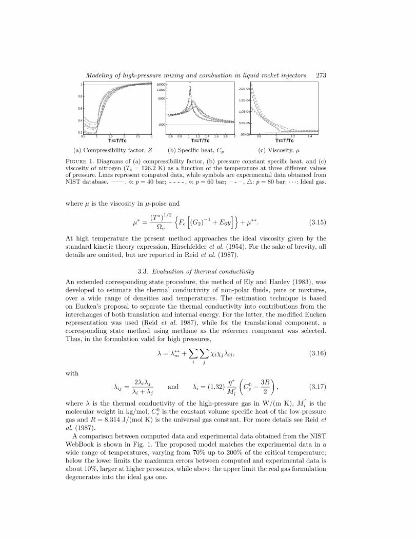
Figure 1. Diagrams of (a) compressibility factor, (b) pressure constant specific heat, and (c)viscosity of nitrogen (Tc = 126.2 K) as a function of the temperature at three different valuesof pressure. Lines represent computed data, while symbols are experimental data obtained fromNIST database. —— , : p = 40 bar; - - - - , : p = 60 bar; – - – , 4: p = 80 bar; · · ·: Ideal gas.

where µ is the viscosity in µ-poise and

µ∗ =(T ∗)1/2

Ωv

Fc

[(G2)

−1+ E6y

]+ µ∗∗. (3.15)

At high temperature the present method approaches the ideal viscosity given by thestandard kinetic theory expression, Hirschfelder et al. (1954). For the sake of brevity, alldetails are omitted, but are reported in Reid et al. (1987).

3.3. Evaluation of thermal conductivity

An extended corresponding state procedure, the method of Ely and Hanley (1983), wasdeveloped to estimate the thermal conductivity of non-polar fluids, pure or mixtures,over a wide range of densities and temperatures. The estimation technique is basedon Eucken’s proposal to separate the thermal conductivity into contributions from theinterchanges of both translation and internal energy. For the latter, the modified Euckenrepresentation was used (Reid et al. 1987), while for the translational component, acorresponding state method using methane as the reference component was selected.Thus, in the formulation valid for high pressures,

λ = λ∗∗m +∑

i

∑

j

χiχjλij , (3.16)

with

λij =2λiλjλi + λj

and λi = (1.32)η∗

M′i

(C0v −

3R

2

), (3.17)

where λ is the thermal conductivity of the high-pressure gas in W/(m K), M′i is the

molecular weight in kg/mol, C0v is the constant volume specific heat of the low-pressure

gas and R = 8.314 J/(mol K) is the universal gas constant. For more details see Reid etal. (1987).

A comparison between computed data and experimental data obtained from the NISTWebBook is shown in Fig. 1. The proposed model matches the experimental data in awide range of temperatures, varying from 70% up to 200% of the critical temperature;below the lower limits the maximum errors between computed and experimental data isabout 10%, larger at higher pressures, while above the upper limit the real gas formulationdegenerates into the ideal gas one.

274 L. Cutrone, M. Ihme & M. Herrmann

4. Combustion model

For the prediction of the heat release and the effect of the density change on the flowfield, a flamelet/progress variable (FPV) model is used (Pierce & Moin 2004). In thisflamelet-based model, a non-premixed flame is considered as an ensemble of laminarflamelets and their chemical state is obtained from the solution of the flamelet equations

−χ2

∂2Yk∂Z2

= ωk , (4.1a)

−χ2

∂2T

∂Z2− χ

2Cp

(∑

k

Cp,k∂Yk∂Z

+∂Cp∂Z

)∂T

∂Z= − 1

Cp

∑

k

hkωk , (4.1b)

where ωk is the chemical production rate per unit mass of species k and the scalardissipation rate is χ = 2αZ∇Z · ∇Z.

In the FPV model, all flame states are parameterized by the mixture fraction and areaction progress parameter λ. The reaction progress parameter is based on a reactivescalar, the progress variable C, and is defined to be independent of the mixture frac-tion. Using this parameter, the state relation, obtained from a flamelet table, for allthermodynamical and chemical variables, denoted by φ = (T, Yi)

T, can be written as

φ = Fφφφ(Z, λ) . (4.2)

The progress variable is a linear combination of some product mass fractions, and canbe obtained from Eq. (4.2) as

C = FC(Z, λ) . (4.3)

The mean scalar quantities φ are obtained using a presumed joint PDF of Z and λ,which are modeled using a beta-distribution and a Dirac-distribution:

φ(Z, Z ′′2, λ) =

∫∫Fφφφ(Z, λ)β(Z; Z, Z ′′2)δ(λ− λ)dλdλ . (4.4)

The application of this model then requires the solution of the transport equation for λ,which is rather difficult. Here, the table is re-interpolated to a different set of independentparameters and λ is replaced by C. The flamelet library then provides the filtered scalars

as function of Z, Z ′′2, and C. In addition to the solution of the Navier-Stokes equations,

the FPV model requires the solution of the following transport equations for Z and Z ′′2,and C:

∂ρZ

∂t+

∂

∂xj(ρujZ) =

∂

∂xj

[(α+ αt

Z)ρ∂Z

∂xj

], (4.5a)

∂ρZ ′′2

∂t+

∂

∂xj(ρujZ ′′2) =

∂

∂xj

[(α+ αt

Z′′2)ρ∂Z ′′2

∂xj

]+ 2ρχ , (4.5b)

∂ρC

∂t+

∂

∂xj(ρujC) =

∂

∂xj

[(α+ αt

C)ρ∂C

∂xj

]+ ρωC , (4.5c)

where Z is the mean mixture fraction, Z ′′2 is the variance of the mixture fraction, C isthe mean progress variable, and α is the equal diffusion coefficient for all species. Thegradient transport assumption for turbulent fluxes is used and the mean scalar dissipationrate, χ, appearing as a sink term in the equation for the variance of the mixture fraction,

is calculated as χ = γε/kZ ′′2 with γ = 2.

Modeling of high-pressure mixing and combustion in liquid rocket injectors 275

Chamber pressure 5.98 MPaTemperature 128.7 K

Density 514.0 kg/m3

Velocity 0.736 m/sReynolds number 23,250

Table 1. RCM01-b test case.

344 BRANAM AND MAYER

The c subscript refers to the centerline or maximum value for theprole and the innity symbol designates the environmentalvalues.By use of this method, the proles are 1.0 at the centerline and zerooutside the jet itself. Nondimensionalizing length measurementsuses the jet diameter d , full width half maximum (FWHM) valuesr1=2 , and axial location as indicated.

Comparing the ow properties in the axial direction requires aslightly differentnondimensionalizingapproach.Density, tempera-ture, and velocity are of particular interest inasmuch as they employthe injectionconditions½0, T0 , and u0 rather than the localcenterlinevalues as shown in the following equations:

½C D .½ ¡ ½1/=.½0 ¡ ½1/

T C D .T1 ¡ T /=.T1 ¡ T0/; uC D u=u0 (4)

Jet Divergence Angle

The jet divergence angle seems to be one of the most highlyconsidered parameters for jet ows. It is easily measured and com-pared with other results. Chehroudi et al.11 provided a compari-son of many different empirical models with available test dataunder various conditions. Of particular interest to this experimentwere the models put forth by Dimotakis12 and Papamoschou andRoshko.13 Dimotakis12 investigated the entrainment of mass owinto the growing shear layer of a freejet. He proposed a vortic-ity growth rate equation (to follow), which depends on veloc-ity and density ratio between the uid ows. For these condi-tions, the velocity ratio is zero, simplifying the following equationconsiderably:

± 0!

D 0:17

(

.1 ¡ u1=u0/£

1 C .½1=½0/12 .u1=u0/

¤

)

£

Á

1 C³

½1

½0

´12

¡

£

1 ¡ .½1=½0/12

¤

f1 C 2:9[.1 C u1=u0/=.1 ¡ u1=u0/]g

!

(5)

Papamoschou and Roshko13 proposed a visual thickness equationfor incompressible, variable-density mixing layers while study-ing the turbulence and compressibility effects in plane shear lay-ers. This relationship uses a convective velocity denition to re-late the difference in the ows. The experimentally determinedconstant (0.17) allows results to be compared with axisymmet-ric jet ows. Again, with velocity ratio zero, the relationshipsimplies to

± 0vis D 0:17

³

1 ¡u1

u0

´

£

1 C .½1=½0/12

¤

£

1 C .u1=u0/.½1=½0/12

¤(6)

Variousmethodscoulddeterminethe spreadingangle from the com-putational models. Direct evaluation of the edge of the shear layerusing a 0.99 rolloff point for temperature, density, and velocitypro-vides a simple method to accomplish this task. This method can becompared with values determined using an FWHM approach. Theedge of the shear layer is difcult to determine from Raman im-ages, and so the procedure is used to determine the location of halfof the maximum value and then the value is multiplied by two, assuggested by Chehroudi et al.11 A similar approach for the compu-tationalmodels also calculateFWHM values to use as a comparisonfor the Raman results. The shadowgraph images allow direct deter-mination of the angle. These pictures clearly show the edge of theshear layer.

Experimental Setup

Figure 2 shows the pressurized chamber with the injector usedin the experiments along with the boundary conditions assumedfor the model. The diameter of the injector is 2.2 mm, and thelength-to-diameterratio is greater than 40 which is expectedto yieldfully developed pipe ow at the injector exit plane. The chamber

is equipped with an electronic heater to keep the wall temperatureconstant.Opticalaccessto thechamberis providedby fourwindows.The temperature of the injected uid is targeted at values between100 and 130 K, the injection velocity can range from 1 to 10 m/s,and the chamber pressure can be as high as 6 MPa. Table 1 showsthe data for our test cases.

The temperature of the injected uid is generally measuredat position 1 (T1 in Fig. 3). Because the test setup includes notemperature regulation system, the injection temperature is variedby starting the injection at the ambient temperature of the injec-tor and the piping. During injection, the piping and the injectorcool down while the injected uid heats up. When the temper-ature of the injected uid reaches its targeted value at T1, theexperiment records the shadowgraph or Raman images. Becausethe time required to take the images is short compared to thetime the injector needs to cool down, the project assumes quasi-steady-state conditions. Nevertheless, there is a certain heat trans-fer from the injector to the uid during the measurement resultingin a temperature difference between T1 and T2 (Fig. 3) depend-ing on the injection conditions. To determine the exact injectionconditions at T2, calibration measurements at this position werenecessary.

A rst approach (T2a) used a thermocoupleas shown on the leftin Fig. 4. The jet is heavily disturbed by the thermocouple, and itis possible the tip of the thermocouple is not completely wettedby the injected nitrogen. Therefore, these measurements were ex-pected to give higher than actual values, providing an upper boundfor the expected temperature. A second series of temperature mea-surements was performed using the setup shown on the right in

Fig. 2 Test chamber.

Fig. 3 Injector.

344 BRANAM AND MAYER

The c subscript refers to the centerline or maximum value for theprole and the innity symbol designates the environmentalvalues.By use of this method, the proles are 1.0 at the centerline and zerooutside the jet itself. Nondimensionalizing length measurementsuses the jet diameter d , full width half maximum (FWHM) valuesr1=2 , and axial location as indicated.

Comparing the ow properties in the axial direction requires aslightly differentnondimensionalizingapproach.Density, tempera-ture, and velocity are of particular interest inasmuch as they employthe injectionconditions½0, T0 , and u0 rather than the localcenterlinevalues as shown in the following equations:

½C D .½ ¡ ½1/=.½0 ¡ ½1/

T C D .T1 ¡ T /=.T1 ¡ T0/; uC D u=u0 (4)

Jet Divergence Angle

The jet divergence angle seems to be one of the most highlyconsidered parameters for jet ows. It is easily measured and com-pared with other results. Chehroudi et al.11 provided a compari-son of many different empirical models with available test dataunder various conditions. Of particular interest to this experimentwere the models put forth by Dimotakis12 and Papamoschou andRoshko.13 Dimotakis12 investigated the entrainment of mass owinto the growing shear layer of a freejet. He proposed a vortic-ity growth rate equation (to follow), which depends on veloc-ity and density ratio between the uid ows. For these condi-tions, the velocity ratio is zero, simplifying the following equationconsiderably:

± 0!

D 0:17

(

.1 ¡ u1=u0/£

1 C .½1=½0/12 .u1=u0/

¤

)

£

Á

1 C³

½1

½0

´12

¡

£

1 ¡ .½1=½0/12

¤

f1 C 2:9[.1 C u1=u0/=.1 ¡ u1=u0/]g

!

(5)

Papamoschou and Roshko13 proposed a visual thickness equationfor incompressible, variable-density mixing layers while study-ing the turbulence and compressibility effects in plane shear lay-ers. This relationship uses a convective velocity denition to re-late the difference in the ows. The experimentally determinedconstant (0.17) allows results to be compared with axisymmet-ric jet ows. Again, with velocity ratio zero, the relationshipsimplies to

± 0vis D 0:17

³

1 ¡u1

u0

´

£

1 C .½1=½0/12

¤

£

1 C .u1=u0/.½1=½0/12

¤(6)

Variousmethodscoulddeterminethe spreadingangle from the com-putational models. Direct evaluation of the edge of the shear layerusing a 0.99 rolloff point for temperature, density, and velocitypro-vides a simple method to accomplish this task. This method can becompared with values determined using an FWHM approach. Theedge of the shear layer is difcult to determine from Raman im-ages, and so the procedure is used to determine the location of halfof the maximum value and then the value is multiplied by two, assuggested by Chehroudi et al.11 A similar approach for the compu-tationalmodels also calculateFWHM values to use as a comparisonfor the Raman results. The shadowgraph images allow direct deter-mination of the angle. These pictures clearly show the edge of theshear layer.

Experimental Setup

Figure 2 shows the pressurized chamber with the injector usedin the experiments along with the boundary conditions assumedfor the model. The diameter of the injector is 2.2 mm, and thelength-to-diameterratio is greater than 40 which is expectedto yieldfully developed pipe ow at the injector exit plane. The chamber

is equipped with an electronic heater to keep the wall temperatureconstant.Opticalaccessto thechamberis providedby fourwindows.The temperature of the injected uid is targeted at values between100 and 130 K, the injection velocity can range from 1 to 10 m/s,and the chamber pressure can be as high as 6 MPa. Table 1 showsthe data for our test cases.

The temperature of the injected uid is generally measuredat position 1 (T1 in Fig. 3). Because the test setup includes notemperature regulation system, the injection temperature is variedby starting the injection at the ambient temperature of the injec-tor and the piping. During injection, the piping and the injectorcool down while the injected uid heats up. When the temper-ature of the injected uid reaches its targeted value at T1, theexperiment records the shadowgraph or Raman images. Becausethe time required to take the images is short compared to thetime the injector needs to cool down, the project assumes quasi-steady-state conditions. Nevertheless, there is a certain heat trans-fer from the injector to the uid during the measurement resultingin a temperature difference between T1 and T2 (Fig. 3) depend-ing on the injection conditions. To determine the exact injectionconditions at T2, calibration measurements at this position werenecessary.

A rst approach (T2a) used a thermocoupleas shown on the leftin Fig. 4. The jet is heavily disturbed by the thermocouple, and itis possible the tip of the thermocouple is not completely wettedby the injected nitrogen. Therefore, these measurements were ex-pected to give higher than actual values, providing an upper boundfor the expected temperature. A second series of temperature mea-surements was performed using the setup shown on the right in

Fig. 2 Test chamber.

Fig. 3 Injector.

Figure 2. Test chamber and injector.

The solution of Eq. (4.4) provides the mean composition Yi that can be used in Eqs.(3.1)–(3.16) in order to calculate density, enthalpy, and the transport properties at highpressure.

5. Mixing test cases

5.1. RCM01b- test case

The RCM01-b test case (Mayer et al. 1998) is a very good benchmark case because itseparates the effect of the real-gas modeling and turbulent mixing from combustion. Itconsists of the simulation of the injection of a dense cryogenic jet of liquid nitrogen ina light and warm environment of gaseous nitrogen. The geometry of the test facility isshown in Fig. 2. The test chamber consists of a cylindrical vessel with an inner diameter of122 mm. The actual length of the vessel is 1000 mm. The injector is located in the centerof the face plate. The injector element’s inner diameter is 2.2 mm. The tube length is 90mm. As the tube length to tube diameter is more than 40, a fully developed turbulentvelocity profile is expected at the end of the tube (point T2). The operating conditionsfor the RCM01-b test are reported at point T1, in Table 1.

The 2-D axysimmetric steady computation has been performed with the flow solverC3NS-DB, using a computational grid with about 30,000 points with an y+

1 < 1 at thewalls. The same simulation was performed on two additional grid levels, one coarser withabout 7,500 points and one finer with about 120,000 points. The results (not shown here)indicate that the intermediate level achieves grid independence. The turbulence modelused is the k − ω model in the low Reynolds number version of Wilcox (1998).

Figures 3(a) and 3(b) show the computed density profiles in two planes orthogonal tothe injection direction. The first one, referring to a section very close to the injectionpoint (x = 11 mm), shows the good agreement between real gas model predictions andexperimental data. Strong discrepancies exist between the ideal gas predictions and the

276 L. Cutrone, M. Ihme & M. Herrmann

R/d

Den

sity

[kq/

m^3

]

-4 -3 -2 -1 0 1 2 3 4

100

200

300

400

500

(a) x/d = 5.

R/d

Den

sity

[kq/

m^3

]

-4 -3 -2 -1 0 1 2 3 450

100

150

200

(b) x/d = 25 .

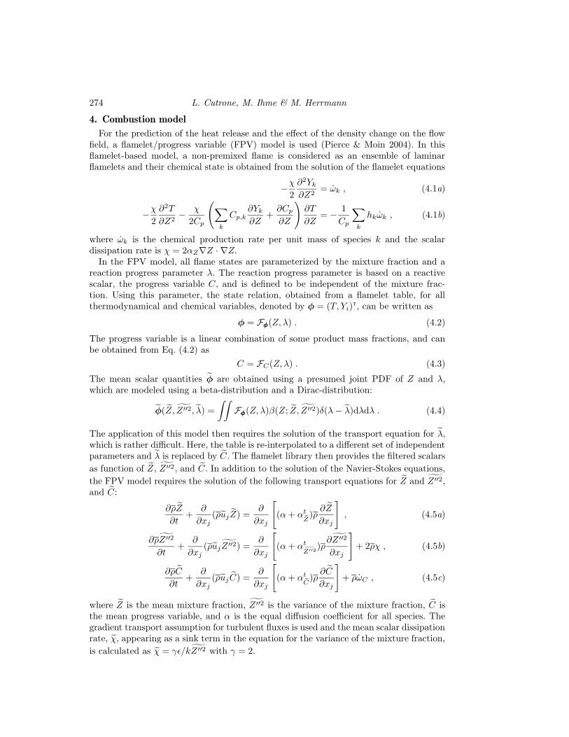
Figure 3. Density profiles: comparison between different levels of real gas corrections: —— Fullcorrection (EOS, thermodynamic and transport data); – - – Partial correction (EOS and ther-modynamic data); - - - - Only EOS correction; – - - – Ideal gas; • Experimental data.

0.095 0.105 0.115 0.125 0.135 0.145 0.155

0.31 0.435 0.56 0.685 0.81 0.935

(a)

0.095 0.105 0.115 0.1251.2 1.8 2.4 3 3.6 4.2 4.8

T=128.96 T=149.82T=139.14CA B

Temperature [K]

Zh

50 100 150 200 250 300 350 400 4501

2

3

4

5

A

B

C

(b)

Figure 4. Computed compressibility factor and specific heat factor (Cpr/Cpid) contours.

experimental data: near the injector, in fact, high-pressure effects are very strong, asclearly shown by the compressibility factor and the ratio between real and ideal specificheats presented in Figs. 4(a)–(b). Moving downstream, the cold nitrogen jet mixes withthe nitrogen of the chamber and warms up: real gas effects decrease, as indicated againin Fig. 4(a), but a non-ideal behavior still exists, as demonstrated by the difference inthe real and ideal gas predicted density profiles presented in Fig. 3(b) at a radial section55 mm downstream of the injection point.

At this location in the computed field, the difference between three levels of approx-imation can be seen: the first one (dash-dotted line) considers only the correction onthe equation of state, the second (dashed line) adds the correction on the thermody-namic data (enthalpy and Cp), while the last one (solid line) computes also the transportproperties in high-pressure condition. The first two levels of approximation fail in thecorrect evaluation of the density profile, especially for the peak value, whereas, if thecomplete real gas model is used (solid line), the difference between the computed andthe experimental density profile reduces.

Finally, Fig. 4(b) shows that the constant pressure specific heat goes through a max-imum: this situation can be handled by the proposed model because it predicts a finitevalue for Cp at the critical point, while theory says that it goes to infinity. In such a way it

Modeling of high-pressure mixing and combustion in liquid rocket injectors 277

Figure 5. A schematic diagram of the rocket shear coaxial injector examined.

is possible to simulate the whole process in which a transition occurs from the subcriticalto supercritical condition, as the in mentioned cases of injection of liquid propellants tohigh-pressure rocket combustion chambers.

5.2. O2-CH4 jet

A schematic diagram of the model injector considered in the simulation of a O2-CH4 jet ispresented in Fig. 5. Co-flowing methane (outer) and oxygen (inner) streams are injectedat the inlet and separated by a 0.3 mm thick LOx post. The inner diameter of the LOx

post is δ =1.2 mm, and that of the methane pipe is 2.4 mm. Fully developed turbulentpipe flow is assumed at the injector outlets. The combustion chamber is initializatedwith gaseous methane at 300 K and 100 bar. The injection velocities of the two streamsare chosen to match the mass-flux ratio in the experiment conducted by Singla et al.(2004). The computational domain includes the injector ducts and part of the combustionchamber; the domain extends downstream of the injector face plate up to a length of 40δ and a radius of 24 δ. The simulation has been performed solving the 2-D axisymmetricRANS equations on a grid with approximately 13,000 grid points. The grid is clusterednear walls, and the first cell near walls is chosen in order to resolve the inertial subrangeof the turbulent boundary layer (y+ < 1). Finally, non-slip adiabatic conditions areenforced along all the solid walls.

In Figs. 6 and 7, the mean density and mean axial velocity are shown along the radialdirection, at different axial locations. The reference data have been obtained by a LEScomputation (Zong & Yang 2005) using a different model for the equation of state. Boththe thermodynamic models have been developed to correctly describe the gas propertiesat high pressure, therefore, the good agreement between the current simulation and theLES confirms that the proposed RANS tool is able to describe correctly the mixing offuel and oxidizer in high-pressure (i.e., supercritical) conditions.

5.3. Reacting O2-CH4 jet

The turbulent combustion model has been tested by performing a simulation of a reactiveO2-CH4 jet: the geometry of the test is similar to that used for the non-reacting test,Fig. 5, but in this case the computational domain is limited only to the mixing regionafter the injectors. The thickness of the LOx post is 0.4 mm, its inner diameter is δ =7mm, while the outer diameter of the methane duct is 8.8 mm.

The chamber is at 100 bar and propellants are injected at 300 K and velocity of 150

278 L. Cutrone, M. Ihme & M. Herrmann

Density, [kg/m3]

y/

0 500 10000

2

4

6

8

10

δ

Density, [kg/m3]

y/

0 500 10000

2

4

6

8

10

δ

Density, [kg/m3]

y/

200 400 600 8000

2

4

6

8

10δ

Density, [kg/m3]

y/

0 500 10000

2

4

6

8

10

δ

Density, [kg/m3]

y/

0 500 10000

2

4

6

8

10

δ

(a) x/δ = 2

Density, [kg/m3]

y/

0 500 10000

2

4

6

8

10

δ

Density, [kg/m3]

y/

0 500 10000

2

4

6

8

10

δ

Density, [kg/m3]

y/

200 400 600 8000

2

4

6

8

10

δ

Density, [kg/m3]

y/

0 500 10000

2

4

6

8

10

δ

Density, [kg/m3]

y/

0 500 10000

2

4

6

8

10

δ

(b) x/δ = 4

Density, [kg/m3]

y/

0 500 10000

2

4

6

8

10

δ

Density, [kg/m3]

y/

0 500 10000

2

4

6

8

10

δ

Density, [kg/m3]

y/

200 400 600 8000

2

4

6

8

10

δ

Density, [kg/m3]

y/

0 500 10000

2

4

6

8

10

δ

Density, [kg/m3]

y/

0 500 10000

2

4

6

8

10

δ

(c) x/δ = 6

Density, [kg/m3]

y/

0 500 10000

2

4

6

8

10

δ

Density, [kg/m3]

y/

0 500 10000

2

4

6

8

10

δ

Density, [kg/m3]

y/

200 400 600 8000

2

4

6

8

10

δ

Density, [kg/m3]

y/

0 500 10000

2

4

6

8

10

δ

Density, [kg/m3]

y/

0 500 10000

2

4

6

8

10

δ

(d) x/δ = 8

Density, [kg/m3]y/

0 500 10000

2

4

6

8

10

δ

Density, [kg/m3]

y/

0 500 10000

2

4

6

8

10

δ

Density, [kg/m3]

y/

200 400 600 8000

2

4

6

8

10

δ

Density, [kg/m3]

y/

0 500 10000

2

4

6

8

10

δ

Density, [kg/m3]

y/

0 500 10000

2

4

6

8

10

δ

(e) x/δ = 10

Figure 6. Radial distribution of density at five axial stations. —— : Current RANSsimulation; • : LES simulation.

Velocity, [m/s]

y/

0 10 20 300

2

4

6

8

10

δ

Velocity, [m/s]

y/

0 10 20 300

2

4

6

8

10

δ

Velocity, [m/s]

y/

0 10 20 300

2

4

6

8

10

δ

Velocity, [m/s]

y/

0 10 20 300

2

4

6

8

10

δ

Velocity, [m/s]

y/

0 10 20 300

2

4

6

8

10

δ

(a) x/δ = 2

Velocity, [m/s]

y/

0 10 20 300

2

4

6

8

10

δ

Velocity, [m/s]

y/

0 10 20 300

2

4

6

8

10

δ

Velocity, [m/s]

y/

0 10 20 300

2

4

6

8

10

δ

Velocity, [m/s]

y/

0 10 20 300

2

4

6

8

10

δ

Velocity, [m/s]

y/

0 10 20 300

2

4

6

8

10

δ

(b) x/δ = 4

Velocity, [m/s]

y/

0 10 20 300

2

4

6

8

10

δ

Velocity, [m/s]

y/

0 10 20 300

2

4

6

8

10

δVelocity, [m/s]

y/0 10 20 300

2

4

6

8

10

δ

Velocity, [m/s]

y/

0 10 20 300

2

4

6

8

10

δ

Velocity, [m/s]

y/

0 10 20 300

2

4

6

8

10

δ

(c) x/δ = 6

Velocity, [m/s]

y/

0 10 20 300

2

4

6

8

10

δ

Velocity, [m/s]

y/

0 10 20 300

2

4

6

8

10

δ

Velocity, [m/s]

y/

0 10 20 300

2

4

6

8

10

δ

Velocity, [m/s]

y/

0 10 20 300

2

4

6

8

10

δ

Velocity, [m/s]

y/

0 10 20 300

2

4

6

8

10

δ

(d) x/δ = 8

Velocity, [m/s]

y/

0 10 20 300

2

4

6

8

10

δ

Velocity, [m/s]

y/

0 10 20 300

2

4

6

8

10

δ

Velocity, [m/s]

y/

0 10 20 300

2

4

6

8

10δ

Velocity, [m/s]

y/

0 10 20 300

2

4

6

8

10

δ

Velocity, [m/s]

y/

0 10 20 300

2

4

6

8

10

δ

(e) x/δ = 10

Figure 7. Radial distribution of velocity at five axial stations. —— : Current RANSsimulation; • : LES simulation.

m/s. A 2-D axisymmetric simulation is performed on a grid with approximately 10,000grid points.

A comparison was provided by the LES results obtained by Ierardo et al. (2004) forthe same test cases. In Fig. 8, the contour-plot of the temperature in both simulationsis shown: the peak value is close to 3400 K for both cases, even if the current simulationuses a flamelet library based on a detailed kinetic reaction scheme (GRIMECH 2.11),while the LES adopts a single-step scheme. Differences arise in the prediction of the heatrelease and in the thickness of the flame: the LES flame diffuses more in the oxygen

Modeling of high-pressure mixing and combustion in liquid rocket injectors 279

(a)

T [K]: 300 702.685 1105.37 1508.05 1910.74 2313.42 2716.11 3118.79

-0.004

0.0

x[m

]

0.005

0.0 0.01 z [m] 0.02 0.03

(b)z [m]

x[m

]

0 0.01 0.02 0.03-0.004

0

0.004

T [K]: 300 565.772 831.544 1097.32 1363.09 1628.86 1894.63 2160.4 2426.17 2691.95 2957.72 3223.49 3489.26T [K]: 300 742.953 1185.91 1628.86 2071.81 2514.77 2957.72 3400.67

-0.004

0.0

x[m

]

0.005

0.0 0.01 z [m] 0.02 0.03

Figure 8. Contours of temperature for the combustion of O2-CH4: (a) LES simulation(Ierardo et al. 2004); (b) current RANS simulation.

Y

Mas

sF

ract

ion

0 0.001 0.002 0.003 0.004 0.0050

0.2

0.4

0.6

0.8

1

(a) x/δ = 0.1

Y

Mas

sF

ract

ion

0 0.001 0.002 0.003 0.004 0.0050

0.2

0.4

0.6

0.8

1

(b) x/δ = 0.5

Y

Mas

sF

ract

ion

0 0.001 0.002 0.003 0.004 0.0050

0.2

0.4

0.6

0.8

1

(c) x/δ = 1.0

Y

Mas

sF

ract

ion

0 0.001 0.002 0.003 0.004 0.0050

0.2

0.4

0.6

0.8

1

(d) x/δ = 2.0

Y

Mas

sF

ract

ion

0 0.001 0.002 0.003 0.004 0.0050

0.2

0.4

0.6

0.8

1

(e) x/δ = 3.0

Y

Mas

sF

ract

ion

0 0.001 0.002 0.003 0.004 0.0050

0.2

0.4

0.6

0.8

1

(f) x/δ = 4.0

Figure 9. Mixture radial composition at six different axial section. —— : YCH4 ;- - - - : YO2 ; – - – : YH2O;· · · : YH2 ; — — : YCO; – - - – : YCO2 .

stream and the heat release is gradual, while in the current simulation the combustionis limited to a very thin layer at the interface between fuel and oxidizer, the heat releaseis very fast, and the flame is still attached to the injector post. Oxygen remains at theoutflow depicted in Fig. 9, where the composition of the flow, at six axial stations, isreported.

6. Conclusions and future work

A self-consistent model is presented for the simulation of monophase supercriticalreacting flows. The model is able to describe the correct behavior of the thermodynamicproperties of a gas mixture for a wide range of temperatures and pressures, and inparticular in the range of interest for the simulation of liquid rocket combustion chambers.

280 L. Cutrone, M. Ihme & M. Herrmann

Some non-reacting test cases have been conducted and the good agreement betweenthe computed data and experimental and numerical data, available in the literature,demonstrates the suitability of the monophase approach to the simulation of supercriticalbi-phase flows. Further investigation is needed to assess the accuracy and the reliabilityof the proposed turbulent combustion models: numerical data available in the literature,allows for a preliminary verification of the code capabilities, but experimental tests are,of course, necessary to achieve final validation.

Acknowledgment

The authors are grateful to Prof. Pitsch for useful suggestions and for help in thegeneration of the flamelet library used in this work.

REFERENCES

Chung, T.H., Lee, L.L. & Starling, K. E. 1984 Applications of the kinetic gastheories and multiparameter correlation for prediction of diluite gas viscosity andthermal-conductivity. Ind. Eng. Chem. Fund. 23, 8–13.

Ely, J.F. & Hanley, H.J.M. 1983 Prediction of transport properties: thermal conduc-tivity of pure fluids and mixtures. Ind. Eng. Chem. Fund. 22, 90–97.

Harstad, K.G., Miller, R.S. & Bellan, J. 2000 Efficient high pressure state equa-tions. Amer. Inst. Chem. Eng. J. 43 , 1675–1706.

Hirschfelder, J.O., Curtiss, C.F. & Bird, R.B. 1954 Molecular Theory of Gasesand Liquids. John Wiley and Sons, New York.

Ierardo, N., Congiunti, A. & Bruno, C. 2004 Mixing and combustion in supercrit-ical O2/CH4 liquid rocket injectors. AIAA Paper 2004-1163.

Mayer, W. et al. 1998 Atomization and breakup of cryogenic propellants under high-pressure subcritical and supercritical conditions. J. Prop. Power. 14, 835–842.

Miller, R., Harstad, K. & Bellan, J. 2001 Direct numerical simulations of super-critical fluid mixing layers applied to heptane-nitrogen. J. Fluid Mech. 436, 1–39.

Peng, D.Y. & Robinson, D.B. 1976 A new two-constant equation of state. Ind. Eng.Chem. Fund. 15, 58–64.

Pierce, C. & Moin, P. 2004 Progress-variable approach for large-eddy simulation ofnon-premixed turbulent combustion. J. Fluid Mech. 504, 73–97.

Prausnitz, D., Lichtenthaler, R. & De Azevedo, E. 1986 Molecular Thermody-namics for Fluid Phase Equation, Prentice-Hall.

Reid, R.C. et al. 1987 The Properties of Gases and Liquids, MGraw-Hill Inc.

Schwer,D. A. 1999 Numerical study of unsteadiness in non-reacting and reacting mix-ing layer. PhD Thesis, The Pennsylvania State University.

Singla, G. et al. 2004 Transcritical Oxygen/transcritical or supercritical Methanecombustion. Proceedings of 30th International Symposium on Combustion, Chicago.

Soave, G. 1972 Equilibrium constants from a modified Redlich-Kwong equation of state.Chem. Eng. Sci. 27, 1197–1203.

Twu, C.H. et al. 1991 A cubic equation of state with a new alpha function and a newmixing rule. Fluid Phase Eq. 69, 33–50.

Wilcox, D. C. 1998 Turbulence Models for CFD. DCW Industries, Inc.

Wilson, G.M. 1964 Vapor-liquid equilibria correlated by means of a modified Redlich-Kwong equation of state. Advanced Cryogenic Eng. 9, 168–176.

Modeling of high-pressure mixing and combustion in liquid rocket injectors 281

Zong, N. & Yang, V. 2005 A numerical study of high-pressure Oxygen/Methane mixingand combustion of a shear coaxial injector. AIAA Paper 2005-0152.