
Modeling of Complex Pentahedron Solar Still Covers to ...
65
Brigham Young University Brigham Young University BYU ScholarsArchive BYU ScholarsArchive Theses and Dissertations 2012-07-05 Modeling of Complex Pentahedron Solar Still Covers to Optimize Modeling of Complex Pentahedron Solar Still Covers to Optimize Distillate Distillate Jeremy D. LeFevre Brigham Young University - Provo Follow this and additional works at: https://scholarsarchive.byu.edu/etd Part of the Mechanical Engineering Commons BYU ScholarsArchive Citation BYU ScholarsArchive Citation LeFevre, Jeremy D., "Modeling of Complex Pentahedron Solar Still Covers to Optimize Distillate" (2012). Theses and Dissertations. 3663. https://scholarsarchive.byu.edu/etd/3663 This Thesis is brought to you for free and open access by BYU ScholarsArchive. It has been accepted for inclusion in Theses and Dissertations by an authorized administrator of BYU ScholarsArchive. For more information, please contact [email protected], [email protected].
Transcript of Modeling of Complex Pentahedron Solar Still Covers to ...

Brigham Young University Brigham Young University
BYU ScholarsArchive BYU ScholarsArchive
Theses and Dissertations
2012-07-05
Modeling of Complex Pentahedron Solar Still Covers to Optimize Modeling of Complex Pentahedron Solar Still Covers to Optimize
Distillate Distillate
Jeremy D. LeFevre Brigham Young University - Provo
Follow this and additional works at: https://scholarsarchive.byu.edu/etd
Part of the Mechanical Engineering Commons
BYU ScholarsArchive Citation BYU ScholarsArchive Citation LeFevre, Jeremy D., "Modeling of Complex Pentahedron Solar Still Covers to Optimize Distillate" (2012). Theses and Dissertations. 3663. https://scholarsarchive.byu.edu/etd/3663
This Thesis is brought to you for free and open access by BYU ScholarsArchive. It has been accepted for inclusion in Theses and Dissertations by an authorized administrator of BYU ScholarsArchive. For more information, please contact [email protected], [email protected].

Modeling of Complex Pentahedron Solar
Still Covers to Optimize Distillate
Jeremy LeFevre
A thesis submitted to the faculty of Brigham Young University
in partial fulfillment of the requirements for the degree of
Master of Science
W. Jerry Bowman, Chair Matthew R. Jones
Christopher A. Mattson
Department of Mechanical Engineering
Brigham Young University
August 2012
Copyright © 2012 Jeremy LeFevre
All Rights Reserved

ABSTRACT
Modeling of Complex Pentahedron Solar Still Covers to Optimize Distillate
Jeremy LeFevre
Department of Mechanical Engineering, BYU Master of Science
This work shows the results of modeling and optimizing pentahedron-shaped covers for
application on a passive solar still. While modeling under the assumption of clear weather in Provo, Utah, United States of America, it was found that two main geometries resulted:
1. A single slope still with fully vertical back and sidewalls and a south face tilted at
37.1°, absorbing a total of 8.98 megajoules of direct solar radiation. 2. A half-pyramid shaped cover with vertical backwall, sidewalls tilted in at 60.6°, and a
south face tilted in at 41.5°, absorbing 9.34 megajoules of direct solar radiation. With improved covers, solar radiation absorbed by the basin can be maximized.
Maximum radiation absorbed will generally indicate maximum still output. In addition, the internal convection of a passive solar still was modeled in order to
compare with existing correlations to find the best convection correlation. The convection was modeled using Fluent 12 (CFD software package) and simulations were run for various geometries and temperatures. It was found that Shruti’s correlation agreed the best with the CFD results. However, another possible correlation is suggested here which accommodates a higher range of Grashof numbers. For a correlation of the form 𝑁𝑢 = 𝐶 · 𝑅𝑎𝑛, it was found that C = 1.02, 0.56, and 0.66, and n = 0.19, 0.24, and 0.24 for cover tilt angles of 15°, 30°, and 45° respectively. Also, Grashof number ranges are 4.0 x 10³ < Gr < 1.9 x 10⁷, 4.0 x 10⁴ < Gr < 1.9 x 10⁸, and 2.1 x 10⁵ < Gr < 1.0 x 10⁹ respectively. Keywords: Jeremy LeFevre, solar, still, distillation, desalination, water purification, thermal

ACKNOWLEDGEMENTS
Several of the faculty members here at BYU have made contributions to this work or
directly to me. It would be an oversight to not briefly acknowledge their help and contributions.
First, thanks to Dr. Bowman for paying my tuition every semester and making sure I had
TA work throughout the year. Also, thanks for lending me your reference materials on a regular
basis and directing the research to be able to accomplish something in the allotted time.
Also, thanks to Dr. Jones and Dr. Mattson for being on my committee and being patient
with me as my research slowly came along. A special thanks to Dr. Jones for all the help with the
heat transfer courses (especially radiative heat transfer, which was vital to this work).
Thanks to Dr. Maynes for lending me research licenses and somehow getting me through
advanced fluids and convective heat transfer.
Thanks to Skyler Chamberlain and Darrel Zeltner for working with me in various courses
and always making time to visit with me every time I stopped by their offices.

v
TABLE OF CONTENTS
LIST OF TABLES ...................................................................................................................... vii
LIST OF FIGURES ..................................................................................................................... ix
NOMENCLATURE ..................................................................................................................... xi
1 Introduction ........................................................................................................................... 1
Desalination .................................................................................................................... 1 1.1
Solar Distillation ............................................................................................................. 1 1.2
Basic Solar Still Model ................................................................................................... 2 1.3
Research .......................................................................................................................... 4 1.4
Objectives ....................................................................................................................... 7 1.5
2 Maximization of Absorbed Radiation for a Pentahedron Cover Geometry for Application in a Passive Solar Still ...................................................................................... 9
Introduction and Review of Literature ............................................................................ 9 2.1
Statement of Intent ........................................................................................................ 10 2.2
2.2.1 Geometries Currently Favored .................................................................................. 10
2.2.2 Geometries Explored in the Current Study ............................................................... 12
2.2.3 Varying Orientation and Shape of the Cover ............................................................ 13
Modeling Process .......................................................................................................... 13 2.3
2.3.1 Solar Radiation Modeling ......................................................................................... 13
2.3.2 Roof-type, Half-pyramid, and Single Slope Stills .................................................... 15
2.3.3 Cover Material’s Effect on the System ..................................................................... 22
2.3.4 Energy Balance and Resulting Heat Transfer ........................................................... 24
Optimization Process .................................................................................................... 24 2.4
2.4.1 Excel Radiation Model ............................................................................................. 24
2.4.2 Optimization Setup ................................................................................................... 25

vi
Optimization Results ..................................................................................................... 27 2.5
2.5.1 Geometries that Performed the Best ......................................................................... 28
2.5.2 Final Optimized Cover Geometries .......................................................................... 29
2.5.3 Visualization of Results ............................................................................................ 29
Conclusion of Optimization Results ............................................................................. 30 2.6
2.6.1 Implications for Engineers ........................................................................................ 31
2.6.2 Suggestions for Future Research .............................................................................. 31
3 Numerical Simulation of Convection in Triangular Cavities to Predict Solar Still Performance ........................................................................................................................ 33
Introduction and Literature Review .............................................................................. 33 3.1
Geometries Studied ....................................................................................................... 35 3.2
CFD Setup and Simulation ........................................................................................... 36 3.3
3.3.1 Mesh Creation ........................................................................................................... 36
3.3.2 Setup in CFD Package .............................................................................................. 37
Grid Dependence .......................................................................................................... 38 3.4
Results ........................................................................................................................... 40 3.5
Conclusions ................................................................................................................... 47 3.6
4 Research Conclusions ......................................................................................................... 49
Radiation Model Trends and Conclusions .................................................................... 49 4.1
CFD Convection Modeling ........................................................................................... 50 4.2
REFERENCES ............................................................................................................................ 51

vii
LIST OF TABLES
Table 2-1: Triangular Face Projected Areas ..........................................................................21
Table 2-2: Trapezoidal Face Projected Areas ........................................................................22
Table 2-3: Optimization Problem Summary ..........................................................................25
Table 2-4: Initial Solar Still Configurations ..........................................................................28
Table 2-5: Optimized Solar Still Configurations ...................................................................30
Table 3-1: CFD Results .........................................................................................................41
Table 3-2: Correlation Coefficients and Details ....................................................................42

ix
LIST OF FIGURES
Figure 1-1: Basin Solar Still Diagram and Terminology .......................................................2
Figure 1-2: Diagram of Energy Processes .............................................................................3
Figure 1-3: Popular Slope Cover Designs (conical still image modified from Watercone [11] ) ................................................5
Figure 1-4: Simple Concept Rendering of a Pentahedron Still..............................................6
Figure 2-1: Single Slope Cover..............................................................................................11
Figure 2-2: Double Slope or Roof Type Cover .....................................................................11
Figure 2-3: Half Pyramid Shaped Cover ...............................................................................12
Figure 2-4: Azimuth, Zenith, and Altitude Angles Defined ..................................................14
Figure 2-5: Radiation Model Geometry .................................................................................15
Figure 2-6: Illustration of the Projected Area on the Basin (Triangular Face Case 1) ..........18
Figure 2-7: Illustration of the Projected Area on the Basin (Trapezoidal Face Case 1) ........18
Figure 2-8: Illustration of the Projected Area on the Basin (Trapezoidal Face Case 4) ........19
Figure 2-9: Projected Triangle ...............................................................................................19
Figure 2-10: Projected Trapezoid ..........................................................................................20
Figure 2-11: Projected Trapezoid ..........................................................................................20
Figure 2-12: Design Space of Single Slope Still ...................................................................26
Figure 2-13: Design Space of Roof Type/Half-Pyramid Still ...............................................27
Figure 2-14: Initial Solar Still Configurations .......................................................................28
Figure 2-15: Optimized Solar Still Configuration .................................................................30
Figure 2-16: Optimized Single Slope ....................................................................................31
Figure 2-17: Optimized Half-Pyramid/Roof Type ................................................................31
Figure 3-1: Comparison of Existing Convection Correlations ..............................................34
Figure 3-2: Geometry and Dimensions of Triangular Cavity ................................................35

x
Figure 3-3: Mesh as Created in Gambit for 30° Triangle ......................................................37
Figure 3-4: Grid Dependence for Conductive Heat Transfer (ΔT = 1 K, θ=30°) ..................39
Figure 3-5: Grid Dependence for Convective Heat Transfer (ΔT = 1 K) ..............................39
Figure 3-6: Comparison of CFD Data with Proposed Correlations for 15°, 30°, and 45° ....43
Figure 3-7: Comparison of Shruti's Correlation with CFD Data (15°) ..................................43
Figure 3-8: Comparison of Shruti's Model with CFD Data (30°) ..........................................44
Figure 3-9: Comparison of Shruti's Correlation with CFD Data (45°) ..................................44
Figure 3-10: Comparison of Dunkle's Correlation with CFD Data .......................................45
Figure 3-11: Comparison of Clark's Correlation with CFD Data ..........................................45
Figure 3-12: Comparison of Farid/Shawaqfeh's Correlation with CFD Data .......................46
Figure 3-13: Comparison of Kumar/Tiwari's Correlation with CFD Data ............................46

xi
NOMENCLATURE
Symbol Description
∀ Volume Enclosed by Cover (m3)
∀basin Volume of Basin (Water) (m3)
∀cover Volume of Cover Material (m3)
A Absorptive coefficient (unitless)
Ab Basin Area (m2)
Ac Cover Area (m2)
Ap,basin, Ai’ Projected area to basin of ith cover surface
(m2)
C Nusselt Correlation Constant Coefficient
cp Specific Heat at Atmospheric Pressure (J/kg
K)
cp,basin Specific Heat of Basin (Water) (J/kg K)
cp,cover Specific Heat of Cover Material (J/kg K)
DAB Mass Diffusivity of Water into Air (m2/s)
�𝑑𝐸𝑑𝑡�𝑏𝑎𝑠𝑖𝑛
Basin Energy Differentiated by Time (W)
�𝑑𝐸𝑑𝑡�𝑐𝑜𝑣𝑒𝑟
Cover Energy Differentiated by Time (W)
g Acceleration Due to Gravity (9.81 m/s2)
Gr Grashof Number (unitless)

xii
h Internal Convective Heat Transfer
Coefficient (W/m2 K)
hm Mass Transfer Coefficient (m/s)
hex External Convective Heat Transfer
Coefficient (W/m2 K)
H Cover Height (m)
hm Convective Mass Transfer Coefficient (m/s)
IN Surface irradiation (W/m2)
ION Extraterrestrial irradiation (W/m2)
k Thermal Conductivity of the Fluid (W/m K)
K1 Beam scattering perturbation factor (unitless)
K2 Background diffuse irradiation (W/m2)
L Basin Length (m)
LC Characteristic Length
Le Lewis Number (unitless)
m Air mass (unitless)
n Nusselt Correlation Exponent Coefficient
𝑛�𝑠𝑢𝑛 Unit Vector in Sun’s Direction (unitless)
𝑛�𝑠𝑢𝑟𝑓𝑎𝑐𝑒,𝑖 Unit Vector Normal to ith Cover Surface
(unitless)
Nu Nusselt Number (unitless)
P Operating Pressure of Still (Pa)
Pr Prandtl Number (unitless)

xiii
q Total Convective Heat Transfer (Watts)
qconvection,in Internal Convective Heat Transfer (Watts)
qconvection,ex External Convective Heat Transfer (Watts)
qevaporation Heat Transfer by Mass Transfer (Watts)
qlosses Heat Losses from Basin (Watts)
qsolar,total,qsolar,absorbed Total solar power absorbed (Watts)
Qsolar,total Total solar energy absorbed (MJ)
qw” Wall Heat Flux (W/m2)
R Reflective coefficient (unitless)
Ra Rayleigh Number (unitless)
Rair Universal Gas Constant of Humid Air (J/kg
K)
S Sutherland Temperature (K)
T Transmissive coefficient (unitless)
t Cover thickness (m)
T∞ Ambient/Surroundings Temperature (K)
Tbasin Basin Temperature (K)
Tcover Cover Temperature (K)
Tfilm Film Temperature (K)
TH Basin Temperature (K)
TL Cover Temperature (K)
TR Linke turbidity factor (unitless)
Tref Reference Temperature (K)

xiv
Ulosses Basin Loss Heat Transfer Coefficient (W/m2)
W Basin Width (m)
x1 X coordinate of projected point 1 (m)
x2 X coordinate of projected point 2 (m)
y1 Y coordinate of projected point 1 (m)
y2 Y coordinate of projected point 2 (m)
α Additional intensity depletion factor
(unitless)
α Absorptivity (unitless)
αbasin Basin Absorptivity (unitless)
γ Azimuth angle (degrees or radians)
∂ Declination angle (degrees or radians)
ΔT Temperature Difference (K)
ε Rayleigh optical thickness of atmosphere
(unitless)
θbasin Basin Tilt Angle (degrees)
θ, θcover Cover Tilt Angle (degrees)
θ, θi , θcover Incident angle (degrees or radians)
θz Zenith angle (degrees or radians)
κ Attenuation coefficient (m-1)
μ Viscosity (Pa s)
μref Reference Viscosity (at Tref) (Pa s)
ρ Reflectivity (unitless)

xv
ρ Density (kg/m3)
ρbasin Density of Basin (Water) (kg/m3)
ρbasin,sat Water Saturation Density at Basin
Termperature (kg/m3)
ρcover Density of Cover Material(kg/m3)
ρcover,sat Water Saturation Density at Cover
Termperature (kg/m3)
τ Transmissivity (unitless)
φ Latitude (degrees)
φcover Cover Tilt Angle (degrees)
χ Refracted angle (degrees or radians)
ω Hour angle (degrees or radians)

1
1 INTRODUCTION
Providing access to clean water is rated as the third greatest challenge of engineering
according to engineeringchallenges.org [1]. The National Academy of Engineers estimates 1 in 6
people in the world do not have adequate water, and as a result, water shortages are responsible
for more deaths globally than war.
The UN’s 2006 Human Development Report [2] estimates that around 2 million children
die each year due to lack of sanitary drinking water. They also claim that the problem itself is
perpetuated due to its negative influence on the economies of developing countries.
Desalination 1.1
Desalination is a popular solution to the world’s water problems because 97% of the
earth’s water is too salty to drink [3]. The earth naturally desalinates water by evaporating ocean
water, leaving the salt in the oceans. When the humidified air cools, the water precipitates and
falls as rain. This natural process has inspired the engineering process known as solar distillation.
Solar Distillation 1.2
Figure 1-1 shows the basic setup of a solar still and also gives some basic terminology. A
typical passive solar still is very simple, composed of three main parts: a basin, a cover, and a
trough that leads to the distillate reservoir. The brackish water is evaporated by solar radiation

2
and the water vapor condenses on the cover. After condensing into large enough drops, the water
collects into the distillate troughs. The setup shown has an inclined basin, but most simple stills
have a basin tilt angle of zero for simplified manufacturing. Tiwari [4] cited multiple sources
showing that the dominant factor in solar still production is insolation. Anything that can
increase the insolation on the basin will improve the performance of the still.
Figure 1-1: Basin Solar Still Diagram and Terminology
Basic Solar Still Model 1.3
Analytical models of solar stills can be derived from a simple energy balance. When
developing any thermal model, there are usually several heat transfer processes to account for. It
is important to model the highest magnitude processes first. In the case of the solar still, a few
main processes dominate the model: solar input, internal convection, internal mass transfer
(evaporation), and basin heat losses. Figure 1-2 shows a diagram illustrating these heat transfer
processes.

3
Figure 1-2: Diagram of Energy Processes
The cover and basin can be treated as control volumes, and energy balances can be
performed on each. The cover yields the equation1
�𝒅𝑬𝒅𝒕�𝒄𝒐𝒗𝒆𝒓
= 𝒒𝒄𝒐𝒏𝒗𝒆𝒄𝒕𝒊𝒐𝒏,𝒊𝒏 + 𝒒𝒆𝒗𝒂𝒑𝒐𝒓𝒂𝒕𝒊𝒐𝒏 − 𝒒𝒄𝒐𝒏𝒗𝒆𝒄𝒕𝒊𝒐𝒏,𝒆𝒙, (1-1)
and the basin yields the equation
�𝒅𝑬𝒅𝒕�𝒃𝒂𝒔𝒊𝒏
= 𝒒𝒔𝒐𝒍𝒂𝒓,𝒂𝒃𝒔𝒐𝒓𝒃𝒆𝒅 − 𝒒𝒄𝒐𝒏𝒗𝒆𝒄𝒕𝒊𝒐𝒏,𝒊𝒏 − 𝒒𝒆𝒗𝒂𝒑𝒐𝒓𝒂𝒕𝒊𝒐𝒏 − 𝒒𝒍𝒐𝒔𝒔𝒆𝒔. (1-2)
Each term can be modeled individually as shown below.
𝒒𝒄𝒐𝒏𝒗𝒆𝒄𝒕𝒊𝒐𝒏,𝒊𝒏 = 𝒉𝑨𝒃(𝑻𝒃𝒂𝒔𝒊𝒏 − 𝑻𝒄𝒐𝒗𝒆𝒓) (1-3)
𝒒𝒆𝒗𝒂𝒑𝒐𝒓𝒂𝒕𝒊𝒐𝒏 = 𝒉𝒎𝑨𝒃(𝝆𝒃𝒂𝒔𝒊𝒏,𝒔𝒂𝒕 − 𝝆𝒄𝒐𝒗𝒆𝒓,𝒔𝒂𝒕) (1-4)
𝒒𝒄𝒐𝒏𝒗𝒆𝒄𝒕𝒊𝒐𝒏,𝒆𝒙 = 𝒉𝒆𝒙𝑨𝒄(𝑻𝒄𝒐𝒗𝒆𝒓 − 𝑻∞) (1-5)
𝒒𝒔𝒐𝒍𝒂𝒓,𝒂𝒃𝒔𝒐𝒓𝒃𝒆𝒅 = 𝜶𝒃𝒂𝒔𝒊𝒏𝑰𝑵 𝒄𝒐𝒔𝜽𝒛 ∑ 𝑻𝒊𝑨𝒊′𝟒𝒊=𝟏 (1-6)
1 All symbols can be found in the NOMENCLATURE.

4
𝒒𝒍𝒐𝒔𝒔𝒆𝒔 = 𝑼𝒍𝒐𝒔𝒔𝒆𝒔𝑨𝒃(𝑻𝒃𝒂𝒔𝒊𝒏 − 𝑻∞) (1-7)
�𝒅𝑬𝒅𝒕�𝒄𝒐𝒗𝒆𝒓
= �𝝆𝒄𝒑∀�𝒄𝒐𝒗𝒆𝒓𝒅𝑻𝒄𝒐𝒗𝒆𝒓
𝒅𝒕 (1-8)
�𝒅𝑬𝒅𝒕�𝒃𝒂𝒔𝒊𝒏
= �𝝆𝒄𝒑∀�𝒃𝒂𝒔𝒊𝒏𝒅𝑻𝒃𝒂𝒔𝒊𝒏
𝒅𝒕 (1-9)
The coefficients h, hm, hex, and Ulosses are typically modeled using correlations found from
experimental data or numerical modeling. In order to have an accurate thermal model, each of
the energy balance terms must be modeled accurately. Specifically, they must capture the major
effects of changing the cover geometry in order to be able to compare designs. In order to
perform an optimization of the still, a model is required that can account for changes in the cover
geometry. Modeling qconvection,in and qsolar,absorbed become particularly important when determining
still performance, and are the subject of this research. Specifically, finding the projected basin
area (Ai’) and the convection coefficient from a Nusselt correlation (Nu = f(Gr,Pr)).
Research 1.4
The analytical model may be used to optimize the geometry and increase total radiation
to a solar still basin. Popular designs of passive solar stills include single slope stills, roof type
stills, and cone shaped stills (see Figure 1-3). Beginning in the early 1970’s, researchers have
looked into optimizing the cover slope angle for single slope stills and roof angle for different
times of the day or year. Single slope and roof type solar stills lose some solar radiation due to
reflection when the sun is not perfectly normal to the cover surface. A different geometry might
improve the production of solar stills by transmitting more radiation. In this work, an analytical
model was created to evaluate the benefits of a complex pentahedron shaped cover versus a
single slope or roof shaped covers (see Figure 1-4).

5
Figure 1-3: Popular Slope Cover Designs (conical still image modified from Watercone [11] )
Much work has been done to optimize the angle of solar still covers and solar collectors
in general. It is generally agreed that the ideal slope for a given collector or cover is the latitude
of the location (for annual energy collected or annual yield). In 2004, Singh [5] experimentally
verified that the optimum angle for both the collector and the cover is the latitude of the location.
Ulgen [6] calculated the optimum solar collector angle for Izmir, Turkey (38 degrees latitude) at
30.3 degrees. For West/East facing sloped solar stills, it was found by Tiwari [7] that the
optimum cover angle was about 55 degrees (probably due to internal convective effects). Effects
such as weather patterns, pollution, convection and condensation loss can also change the ideal

6
angles mentioned above (for example the optimum for Izmir, Turkey, deviates about 8 degrees
from the latitude).
Figure 1-4: Simple Concept Rendering of a Pentahedron Still
Pentahedrons are not totally new designs, and Sayigh [8,9] has done some experiments
comparing dome covers to pyramid shaped covers. In his research, he found that a pyramid
shaped cover produced more distillate in an active still setup (warm water was pumped through
the basin trays). Fath [10] found from experimental data that pyramid type stills are less
economical than single slope stills. However, annual production was comparable, suggesting that
if the angles of the different faces were optimized to improve inlet of solar radiation, production
might be increased.
Another item of interest in the solar distillation community is finding convection
correlations to better predict still performance for a variety of conditions. A difficulty that arises
when changing the cover geometry is the effect that it has on the internal convection. While

7
many correlations exist, most fail to account directly for the change in relationship between the
Grashof and Nusselt number as the cover shape changes.
Objectives 1.5
The goals for this research were:
1. Modeling three types of solar still covers, a single slope, a roof type, and a complex
pentahedron.
2. Compare the radiation absorbed by the basin for any given day of the year for each still
based on irradiance data and solar altitude and azimuth angles.
3. Find geometric parameters that optimize each cover type for maximum solar radiation
capture.
4. Perform an analysis that predicts the convection coefficients for different cover
geometries to find a relationship between Nusselt and Grashof for those geometries.

9
2 MAXIMIZATION OF ABSORBED RADIATION FOR A PENTAHEDRON COVER GEOMETRY FOR APPLICATION IN A PASSIVE SOLAR STILL2
Introduction and Review of Literature 2.1
Solar still cover geometry is always a topic of interest when it comes to designing the
best possible solar still. Several different geometries have been explored but no real consensus to
the best geometry has ever been decided upon (perhaps because several parameters can favor
certain geometries under certain conditions). Ismail built and tested a hemispherical solar still
and was able to achieve outputs from 2.8 to 5.7 L/m2 per day under summer climatic conditions
in Dhahran [12]. Minasian constructed and tested a conical solar still with a wick parallel to the
cover, instead of a basin. It was found to produce from 2 to 4 L/m2 per day in Baghdad over the
year [13]. Tiwari conducted a test of fiber reinforced covers which compared the performance of
the single slope cover to the double slope cover (roof type) directly, and found that season was
the main factor in determining which geometry to use. Findings indicated that the double slope
produced 0.7 to 1.15 L/m2 per day during winter and 2.48 to 2.85 L/m2 per day during summer.
The single slope produced 0.74 to 1.10 L/m2 per day during winter and 2.21 to 2.40 L/m2 per day
during summer [14]. Finally, Fath has done a large amount of work on pyramid shaped covers,
which were found to produce about the same amount of distillate per day as a single slope still
(2.6 L/m2, the annual average for Aswan, Egypt) [10]. This work looks at a direct comparison of
three different cover geometries and optimizes each for conditions in Provo, Utah, United State
of America. 2 Chapter submitted for publishing in Desalination.

10
Statement of Intent 2.2
Three main cover geometries, discussed in this paper, have become the most widely used
and studied for passive, basin type solar stills. These include single slope, roof type, and pyramid
shaped covers. The main objective of this research was determining the geometry that would
maximize solar radiation to the basin. The cover geometry that optimizes solar radiation to the
basin would indicate the best candidate for application in a solar still. On the other hand, the
candidate that can produce the highest amount of distillate per day per unit cost could be a good
candidate as well. The three geometries studied are illustrated in Figures 2-1 to 2-3.
2.2.1 Geometries Currently Favored
Currently, the most commonly used solar still is the single slope configuration. It’s a
simple design and abundant research [15-17] has been done to evaluate its performance at
various locations under various climatic conditions. For this configuration, the cover faces south
(For this work, the still was assumed to be located in the northern hemisphere). One of the most
famous solar stills (built by Charles Wilson near Las Salinas, Chile) appears to have been a
single slope configuration [18]. Probably the next most popular cover type is the roof type
(sometimes called double slope). In this configuration, the covers face east and west. Roof type
covers typically have reduced performance at high latitudes or during the winter. Recently, there
has been increasing interest in pyramid shaped stills [10, 19-20]. The faces of pyramid stills face
all four directions (north, south, east, and west).

11
Figure 2-1: Single Slope Cover
Figure 2-2: Double Slope or Roof Type Cover

12
Figure 2-3: Half Pyramid Shaped Cover
2.2.2 Geometries Explored in the Current Study
The current study used variations on the three covers mentioned above. However, each
geometry was allowed to vary within certain parameters. The following describes how they were
allowed to vary.
Roof-type (double slope, east-west facing) solar stills studied in this work have two sides
both inclined at an angle φ to the horizontal, and a front face that could be vertical (as a
traditional double slope cover) or could be inclined at an angle θ so long as the sides remain
trapezoidal. The back face is vertical (Figure 2-2).
The half-pyramid, Figure 2-3, is basically a pyramid shape cut in half, with the cut face
oriented toward the north. The half-pyramid was chosen instead of a full pyramid because over
the course of the year, very little or no direct radiation will enter the rear surface of the cover, so
it is less beneficial to try to orient it favorably to the sun (especially during winter or at high
latitudes).
A single slope still is basically shaped like a wedge. Typically a single slope still has an
inclined front face with vertical sidewalls. The cover has been modified in this case to allow the

13
sides to collapse inward such that their tilt angle is φ, as long as the front face remains
trapezoidal (Figure 2-1).
2.2.3 Varying Orientation and Shape of the Cover
The cover’s faces (sides and front) were tilted and altered to optimize the total solar
radiation to the basin. All three geometries were optimized to find which configuration allowed
for the most radiation to the basin.
Modeling Process 2.3
Modeling the radiation through the cover of a solar still required several calculations.
Finding the radiation to the basin was broken down into three main steps: Modeling the direct
solar radiation source, modeling projected basin areas, and modeling the properties of the cover
material.
2.3.1 Solar Radiation Modeling
The first major step to finding the solar radiation to the basin was to accurately model the
irradiation provided by the sun at the relevant time of day and day of year. For a solar still, this
required a model of the solar irradiation over the entire course of the day. The general model
used here was from Tiwari’s text [4].
The irradiation and the direction of the sun depends on the time of year, as well as the
time of day. First, the time of year was determined, then the position of the sun was determined
over the course of the defined day. For the current study, the maximum annual average was
desired, so the autumnal equinox was selected (which will yield the same optimum as the annual
average).

14
Figure 2-4: Azimuth, Zenith, and Altitude Angles Defined
With the day of the year fixed, the sun’s position is defined by sweeping out two angles
across the sky: the zenith angle and the azimuth angle (see Figure 2-4). Zenith angle (θz) is
defined as the angle between the sun and the vertical direction. Azimuth angle (γ) is measured
between the vector produced by projecting the direction of the sun to the horizontal (in other
words, the NSEW direction of the sun) and a vector that points in the north direction along the
horizontal. Equations for both have been developed based on the geographic location (φ,
latitude), time of year (δ, declination angle), and time of day (ω, hour angle) [4].
𝜽𝒛 = 𝒄𝒐𝒔−𝟏[𝒄𝒐𝒔 𝝓 𝒄𝒐𝒔 𝜹 𝒄𝒐𝒔𝝎 + 𝒔𝒊𝒏 𝜹 𝒔𝒊𝒏𝝓] (2-1)
𝐜𝐨𝐬 𝜸 = �𝐬𝐢𝐧𝜹 𝐜𝐨𝐬𝝓−𝐜𝐨𝐬𝝎𝐜𝐨𝐬 𝜹 𝐬𝐢𝐧𝝓
𝐜𝐨𝐬𝜶, 𝒊𝒇 𝐬𝐢𝐧𝝎 < 𝟎
𝐜𝐨𝐬𝝎𝐜𝐨𝐬 𝜹 𝐬𝐢𝐧𝝓−𝐬𝐢𝐧𝜹 𝐜𝐨𝐬𝝓𝐜𝐨𝐬𝜶
, 𝒊𝒇 𝐬𝐢𝐧𝝎 > 𝟎 (2-2)

15
Figure 2-5: Radiation Model Geometry
The magnitude of solar irradiation depends on both the time of year, the time of day, and
the current atmospheric conditions. Probably the most difficult variables to model are the current
atmospheric conditions, as they are free to vary over the course of the day. In this study,
atmospheric conditions were assumed to be clear and non-hazy (which lead to assuming
parameters TR = 3.81, α = 0.08, K1 = 0.32, and K2 = 17.50) for the irradiation model [4]. Direct
irradiation (W/m2) is given
𝑰𝑵 = 𝑰𝑶𝑵𝒆−𝒎 𝜺 𝑻𝑹+ 𝜶 (2-3)
where m and ε are dependent on zenith angle. Then, direct irradiation must be multiplied by
cos(θi) to find the component normal to the surface of interest (where θi is the incident angle to
the surface, Figure 2-5). In the case illustrated in Fig. 2-4, the basin normal is vertical, so θi = θz.
2.3.2 Roof-type, Half-pyramid, and Single Slope Stills
Three types of still covers were treated in this study, as mentioned earlier.
All three covers were placed over a horizontal surface of arbitrary width (W) and length
(L) which were assumed to be 1 meter each for the current analysis. The tilt angle of both the

16
front face (oriented south) and the side faces of the single slope cover and roof-type cover could
change during optimization, to the point where they would effectively become a half-pyramid.
The other limiting case was where the tilt angles were 90° for the triangular side surfaces. The
north oriented surfaces were all maintained vertical and not allowed to vary.
Ultimately the direct portion of radiation that gets through a cover surface becomes a
projection of that shape to the basin. Another way of thinking about this is to pretend that a cover
surface is replaced by an opaque surface, and the shadow falls on the ground where the projected
area lies. The intersection of the shadow with the basin area is the area that has the potential to
absorb direct radiation from the same cover surface. See Figures 2-6 to 2-8 for an illustration of
this idea.
Points (x1, y1) and (x2, y2), shown in Figs. 2-9 to 2-11, are projections of the points
corresponding to the elevated corners of a given face.
A triangular surface and a trapezoidal surface will leave different projected areas on the
basin. Several different shapes are possible depending on the orientation of the sun. For the
triangular surface, the equation that determines the projected basin area depends on which region
the projected tip point falls within (Figure 2-9). As a result, there are six possible shapes and
corresponding equations for the projected basin area. For example, the projected basin area in
case 1 would be
𝑨𝒑,𝒃𝒂𝒔𝒊𝒏 = 𝒙𝟏𝑾𝟐
𝟐𝒚𝟏. (2-4)
Deriving this expression is simply a matter of finding the intersection area. In this case, you can
imagine two similar right triangles, one with a corner at (x1,y1), and one with a corner on the
border of regions 1 and 6. The area of any triangle is given
𝑨𝒕𝒓𝒊𝒂𝒏𝒈𝒍𝒆 = 𝟏𝟐𝑯𝒆𝒊𝒈𝒉𝒕 ∙ 𝑩𝒂𝒔𝒆, (2-5)

17
then the height can be found by the similar triangles,
𝒚𝟏𝑯𝒆𝒊𝒈𝒉𝒕
= 𝒙𝟏𝑾
. (2-6)
Then, the base is simply W.
For a trapezoidal surface, the shape of the projected basin area requires the projection of
two points. The shape formed on the basin depends sometimes on the position of one of the
points and sometimes the other. There are a total of eight shapes possible and therefore eight
equations. Case 1 for the trapezoid shows that the projected basin area would be
𝑨𝒑,𝒃𝒂𝒔𝒊𝒏 = 𝒙𝟐𝑾𝟐
𝟐𝒚𝟐 (2-7)
until the red lines shown in Figure 2-10 cross. Case 4 for the trapezoid shows that the projected
basin area would be
𝑨𝒑,𝒃𝒂𝒔𝒊𝒏 = 𝟏𝟐𝑳 �𝟐𝑾 + 𝑳(𝑾+𝒚𝟏)
𝒙𝟏�, (2-8)
which holds as long as −𝑥1𝑊+𝑦1
≥ 𝐿𝑊
, 𝑥1 ≤ −𝐿 𝑎𝑛𝑑 𝑦2 ≥ 0.

18
Figure 2-6: Illustration of the Projected Area on the Basin (Triangular Face Case 1)
Figure 2-7: Illustration of the Projected Area on the Basin (Trapezoidal Face Case 1)

19
Figure 2-8: Illustration of the Projected Area on the Basin (Trapezoidal Face Case 4)
Figure 2-9: Projected Triangle

20
Figure 2-10: Projected Trapezoid
Figure 2-11: Projected Trapezoid

21
Table 2-1: Triangular Face Projected Areas
Case/Region Area Constraints
1 𝐴′ =12𝑊𝐿
𝑥1𝑦1𝑊𝐿
𝑦1 < −𝑊,𝑥1𝑦1
<𝐿𝑊
2 𝐴′ =12𝐿 �2𝑊 −
𝑦1𝐿𝑥1� 𝑦1 ≤ −𝑊,
𝑥1𝑦1≥𝐿𝑊
3 𝐴′ =12𝐿 �𝑊 +
𝑊(𝑥1 + 𝐿)𝑥1
� 0 > 𝑦1 > −𝑊, 𝑥1 < −𝐿
4 𝐴′ =12𝐿 �2𝑊 +
𝐿(𝑦1 + 𝑊)𝑥1
� 𝑦1 ≥ 0,−𝑥1
𝑦1 + 𝑊≥
𝐿𝑊
5 𝐴′ =12𝑊𝐿
−𝑥1𝑦1 + 𝑊
𝑊𝐿
𝑦1 > 0,−𝑥1
𝑦1 + 𝑊<
𝐿𝑊
6 𝐴′ =12
(−𝑥1)𝑊 0 ≥ 𝑦1 ≥ −𝑊, 0 ≥ 𝑥1 ≥ −𝐿

22
Table 2-2: Trapezoidal Face Projected Areas
Case/Region Area Constraints
1 𝐴′ =12𝑊𝐿
𝑥2𝑦2
𝑦2 ≤ −𝑊,𝑥2𝑦2
<𝐿𝑊
2 𝐴′ =12𝐿 �2𝑊 −
𝑦2𝐿𝑥2
� 𝑥1 ≤ −𝐿,𝑦1 ≤ −𝑊,𝑥2𝑦2
≥𝐿𝑊
3 𝐴′ = 𝐿𝑊 �1 −12𝑦2𝑥2
+12𝑊 + 𝑦1𝑥1
� 0 > 𝑦1 > −𝑊, 0 > 𝑦2 > −𝑊,
𝑥1 < −𝐿, 𝑥2 < −𝐿
4 𝐴′ =12𝐿 �2𝑊 +
𝐿(𝑦1 + 𝑊)𝑥1
� 𝑥1 ≤ −𝐿,𝑦2 ≥ 0,−𝑥1
𝑦1 + 𝑊≥
𝐿𝑊
5 𝐴′ =12𝑊𝐿
−𝑥1𝑦1 + 𝑊
𝑦1 ≥ 0,−𝑥1
𝑦1 + 𝑊<
𝐿𝑊
6 𝐴′ =12
(−𝑥2)(2𝑊 + 𝑦2) 0 ≥ 𝑦2 ≥ −𝑊, 0 ≥ 𝑥2 ≥ −𝐿,𝑦1 < −𝑊
7 𝐴′ =12
(−𝑥2)(𝑊 + 𝑦2 − 𝑦1) 0 ≥ 𝑦2 ≥ −𝑊, 0 ≥ 𝑥2 ≥ −𝐿,
0 ≥ 𝑦1 ≥ −𝑊, 0 ≥ 𝑥1 ≥ −𝐿
8 𝐴′ =12
(−𝑥2)(𝑊− 𝑦1) 0 ≥ 𝑦1 ≥ −𝑊, 0 ≥ 𝑥1 ≥ −𝐿,𝑦2 > 0
2.3.3 Cover Material’s Effect on the System
The cover material plays an important role. If the cover material didn’t have directional
properties (diffuse transmitter), the cover geometry wouldn’t affect the radiation reaching the
basin. However, this model was made to study the directional properties of the cover material
and how they affect the total radiation reaching the basin.
For the preliminary study, the cover was assumed to be made of glass. After spectrally
averaging the index of refraction, it was found that for solar radiation, glass has an average index

23
of refraction of 1.458. It was also assumed that the attenuation coefficient of the glass was 1 x
10-4 m-1 for the solar spectrum. The glass was assumed to be 5 mm thick for every surface.
As found in the literature [21], the cover was modeled using electromagnetic wave
theory. Using the index of refraction, the reflectivity was defined
𝝆 = 𝟏𝟐�𝒔𝒊𝒏
𝟐(𝜽−𝝌)𝒔𝒊𝒏𝟐(𝜽+𝝌) + 𝒕𝒂𝒏𝟐(𝜽−𝝌)
𝒕𝒂𝒏𝟐(𝜽+𝝌)� (2-9)
𝒘𝒉𝒆𝒓𝒆 𝝌 = �𝒔𝒊𝒏−𝟏(𝒏𝒔𝒊𝒏𝜽) 𝒇𝒐𝒓 𝒏𝒔𝒊𝒏𝜽 ≤ 𝟏
𝟎 𝒇𝒐𝒓 𝒏𝒔𝒊𝒏𝜽 > 𝟏
The absorptivity and transmissivity are then given
𝜶 = 𝟏 − 𝝆 − 𝝉 𝒂𝒏𝒅 𝝉 = 𝒆−𝜿𝒕
𝐜𝐨𝐬𝝌 (2-10)
where t is the thickness of the cover, and κ is the attenuation coefficient [22].
For a finite slab of semitransparent material, the effective reflection, absorption, and
transmission coefficients were needed. From Siegel and Howell [22], the effective transmission
coefficient is
𝑻 = 𝝉(𝟏−𝝆)(𝟏−𝝆𝟐)(𝟏+𝝆)(𝟏−𝝆𝟐𝝉𝟐)
, (2-11)
the effective reflection coefficient is
𝑹 = 𝝆(𝟏 + 𝝉𝑻) , (2-12)
and the effective absorption coefficient is
𝑨 = (𝟏−𝝆)(𝟏−𝝉)(𝟏−𝝆𝝉)
. (2-13)

24
2.3.4 Energy Balance and Resulting Heat Transfer
Now that the solar angles, the solar irradiation, the projected basin areas, and the
transmission coefficients are known for each of the cover surfaces, the total radiation (qsolar,total)
to the basin was found (index i represents the surface).
𝒒𝒔𝒐𝒍𝒂𝒓,𝒕𝒐𝒕𝒂𝒍 = ∑ 𝑰𝑵𝑻𝒊𝑨𝒊′ 𝐜𝐨𝐬 𝜽𝒛𝟒𝒊=𝟏 = 𝑰𝑵 𝐜𝐨𝐬 𝜽𝒛 ∑ 𝑻𝒊𝑨𝒊′𝟒
𝒊=𝟏 (Watts) (2-14)
Optimization Process 2.4
For the optimization process, the total solar radiation to the basin (qsolar,total, W) was
integrated over the entire day to find the total energy absorbed, Qsolar,total (MJ). This predicted
which cover performed the best in terms of total energy absorbed by the basin (in this model, the
basin was simply assumed to be black).
2.4.1 Excel Radiation Model
Microsoft Excel 2010 was used to make a spreadsheet that calculated the total daily
energy absorbed. The results of qsolar,total were integrated numerically with the trapezoid rule and
a step size of 60 seconds to yield Qsolar,total. The optimization was done using Excel’s solver add-
in.

25
Table 2-3: Optimization Problem Summary
Optimization Problem Setup Find the values of θ and φ that maximize 𝑄𝑠𝑜𝑙𝑎𝑟,𝑡𝑜𝑡𝑎𝑙 = ∫ 𝐼𝑁 cos𝜃𝑧
24 ℎ𝑜𝑢𝑟𝑠0 ∑ 𝑇𝑖𝐴𝑖′4
𝑖=1 𝑑𝑡 where 𝐼𝑁 = 𝑓(𝑡) (see equation 2-3)
𝜃𝑧 = 𝑓(𝑡) (see equation 2-2) 𝜃𝑖 = 𝑓(𝜃𝑐𝑜𝑣𝑒𝑟 ,𝜑𝑐𝑜𝑣𝑒𝑟 , 𝑡) = cos−1�𝑛�𝑠𝑢𝑛 ∙ 𝑛�𝑠𝑢𝑟𝑓𝑎𝑐𝑒,𝑖�
𝑇𝑖 = 𝑓(𝜃𝑖) (see equation 2-11) 𝐴𝑖 = 𝑓(𝜃𝑐𝑜𝑣𝑒𝑟,𝜑𝑐𝑜𝑣𝑒𝑟, 𝑡) (see Tables 2-1 and 2-2)
Single Slope Constraints Roof Type/Half-Pyramid Constraints
𝑊 = 1 𝑚𝑒𝑡𝑒𝑟 𝐿 = 1 𝑚𝑒𝑡𝑒𝑟 1° ≤ 𝜃 ≤ 89° 1° ≤ 𝜑 ≤ 90°
2𝐻tan𝜑
< 𝑊
𝑊 = 1 𝑚𝑒𝑡𝑒𝑟 𝐿 = 1 𝑚𝑒𝑡𝑒𝑟 1° ≤ 𝜃 ≤ 90° 1° ≤ 𝜑 ≤ 89°
𝐻tan 𝜃
≤ 𝐿
2.4.2 Optimization Setup
The model was set up to vary each geometry according to the constraints given in section
3.2 above. GRG nonlinear algorithm was chosen. Automatic variable and objective scaling was
used to keep the optimization process as simple as possible. Forward difference approximation
was used for calculation of all derivatives. Once the geometric constraints were properly added,
the solver iterated until reaching the global maximum (depending on the starting point, usually
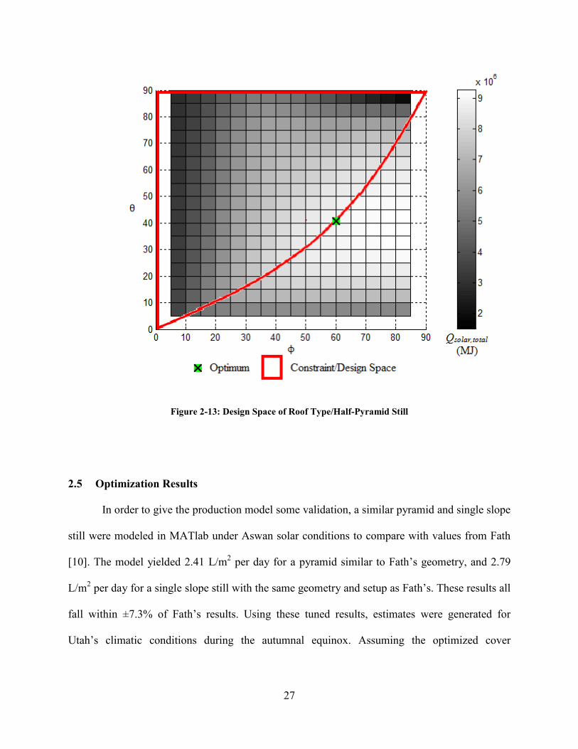
less than 10 iterations were required). To verify the global maximums, the design spaces and
optimums are shown in Figures 2-12 and 2-13. Table 2-3 shows the setup of the optimization
problem.

26
Figure 2-12: Design Space of Single Slope Still
27
Figure 2-13: Design Space of Roof Type/Half-Pyramid Still
Optimization Results 2.5
In order to give the production model some validation, a similar pyramid and single slope
still were modeled in MATlab under Aswan solar conditions to compare with values from Fath
[10]. The model yielded 2.41 L/m2 per day for a pyramid similar to Fath’s geometry, and 2.79
L/m2 per day for a single slope still with the same geometry and setup as Fath’s. These results all
fall within ±7.3% of Fath’s results. Using these tuned results, estimates were generated for
Utah’s climatic conditions during the autumnal equinox. Assuming the optimized cover

28
geometries, the half-pyramid would produce 1.36 L/m2 and the single slope would produce 1.23
L/m2 (within 10% of each other).
2.5.1 Geometries that Performed the Best
The geometry that outperformed all the others in terms of radiation reaching the basin
was the single slope cover (wedge). The pyramid was not far behind, only about 3.9% less
radiation arrived at the basin for the pyramid shape. Geometries resembling the roof type cover
were generally unfavorable because reflective losses were higher than the other geometries. The
initial geometries chosen show this general trend (Figure 2-14, Table 2-4).
Figure 2-14: Initial Solar Still Configurations
Table 2-4: Initial Solar Still Configurations
Still Type South Face Tilt (°) East/West Face Tilt (°) Energy Absorbed by Basin (MJ)Roof 57.3 60.2 8.04Pyramid 56.3 71.6 8.41Wedge 45 80.2 8.92

29
2.5.2 Final Optimized Cover Geometries
All three cover optimization processes produced valuable results for getting the best
cover geometry (in terms of radiation). The side faces of the single slope cover became vertical,
and the south face tilted at an angle of 37.1°. This shows that the south face contributes the most
to the total radiation hitting the basin.
The half-pyramid only changed its height, since the faces were all constrained to meet at
a point. The side angles converged to 60.6° with the horizontal and the south face tilted at 41.5°
at the end of the optimization.
The roof type cover aligned its south face to 41.5°, and then the height of the still
increased until the sides became triangles. The side faces were tilted at 60.6° at the end of the
optimization process, so essentially it evolved to become identical to the half-pyramid. The
optimizations were performed for winter and summer solstices as well, see Table 2-5.
2.5.3 Visualization of Results
The results of the optimization study are shown in Figure 2-15. The radiant power
absorbed by an uncovered black plate is shown, along with the optimized single slope, half-
pyramid, and roof type covers. Note that while the peak of the optimized single slope is higher,
the optimized pyramid is broader. The dips represent where the direct radiation reaches the
Brewster angle for one or more of the surfaces. Overall, there is slightly more area under the
single slope’s curve than the pyramid’s or roof’s curve. Figures 2-16 and 2-17 show the two
optimum cover geometries for the Provo, Utah conditions described previously.

30
Figure 2-15: Optimized Solar Still Configuration
Table 2-5: Optimized Solar Still Configurations
Conclusion of Optimization Results 2.6
For the optimization of solar radiation absorbed, the optimized single slope cover
performed better than the optimized half-pyramid, but the difference in total energy absorbed
was about 3.9%.
Still Type Season South Face Tilt (°) East/West Face Tilt (°) Energy Absorbed by Basin (MJ)Roof Vernal Equinox 41.6 60.6 8.98
Summer Solstice 17.2 31.8 15.8Autumnal Equinox 42.4 61.3 8.68Winter Solstice 84 78 2.45Average 46.3 57.925 8.9775
Pyramid Vernal Equinox 41.5 60.6 8.98Summer Solstice 18.4 33.6 15.8Autumnal Equinox 42.1 61.1 8.68Winter Solstice 83.8 77.8 2.45Average 46.45 58.275 8.9775
Wedge Vernal Equinox 37.1 90 9.34Summer Solstice 16.1 90 15.8Autumnal Equinox 37.2 90 9.05Winter Solstice 59.4 90 2.56Average 37.45 90 9.1875

31
2.6.1 Implications for Engineers
For solar distillation, a single slope cover and a half pyramid cover will perform nearly
the same. As a result, output of each will be nearly the same.
Figure 2-16: Optimized Single Slope
Figure 2-17: Optimized Half-Pyramid/Roof Type
2.6.2 Suggestions for Future Research
The model described in this article gives a reasonable approximation of the radiation
arriving at the basin, but the model neglects the effects of internal reflections. As radiation
coming in one face of the cover eventually arrives at another cover surface, a portion of that
radiation will be transmitted and another portion will be reflected back to another face of the
cover or even the basin. This would probably increase the amount of radiation arriving at the
basin, and should be considered as a topic of future studies. Also, future efforts could include the

32
effects of varied weather conditions, as cloudy conditions increase diffuse radiation and decrease
the direct component. This could yield a different optimized geometry when cover to basin
viewfactors are taken into consideration. Finally, a convection model that accurately takes into
account the possible variations in still cover geometry could yield more accurate results for
predicting the actual production.

33
3 NUMERICAL SIMULATION OF CONVECTION IN TRIANGULAR CAVITIES TO PREDICT SOLAR STILL PERFORMANCE3
Introduction and Literature Review 3.1
Accurately calculating the heat and mass transfer within a solar still is always of interest
to designers of solar stills. Without accurate convection correlations, there cannot be accurate
predictions of the total distillation (using the heat and mass transfer analogy). The heat and mass
transfer analogy can be related using the Lewis number, thermal conductivity, and mass
diffusivity. The relationship is given
𝒉𝒎 = 𝒉𝑫𝑨𝑩𝑳𝒆𝒏
𝒌. (3-1)
One of the first to study convection in cavities as it relates to solar distillation was
Dunkle, who found C = 0.075 and n = 1/3 for a correlation of the form
𝑵𝒖 = 𝑪 · (𝑮𝒓𝑷𝒓)𝒏 = 𝑪 · 𝑹𝒂𝒏 [23]. (3-2)
Clark came up with a similar correlation, except he extended the range to cover lower Grashof
Numbers and divided the coefficients into laminar and turbulent regions [24]. Shawaqfeh and
Farid found a fit with C = 0.067 and n = 1/3, also very similar to Dunkle’s results. Kumar and
Tiwari used regression to find C = 0.0322 and n = 0.4144 for Grashof numbers ranging in the
millions [25]. Finally, probably the most extensive work for triangular cavities was completed
by Shruti and Tiwari, in which coefficients were found for triangular geometries at 15°, 30°, and
3 Chapter submitted for publishing in Desalination.

34
45° [26, 27]. Table 3-2 summarizes coefficients and Grashof ranges for the mentioned works.
The characteristic length for these correlations is defined as
𝑳𝑪 = ∀𝑨𝒃
= 𝑯𝟐
(3-3)
Figure 3-1: Comparison of Existing Convection Correlations
While there are multiple correlations that have been developed for predicting the
convection and mass transfer coefficient, they are not always in good agreement (see Figure 3-1)
and some have limited Grashof number range. For example, Shruti’s correlations predict higher
Nusselt number at higher Grashof numbers than all the other correlations. On the other hand,
Farid and Shawaqfeh predict lower values of Nusselt over a wide range compared to all other
correlations. All of the previous correlations were experimentally measured using specific cover
geometries, and may be less accurate for cover geometries that are different than the original
cover for which they were developed. As a result, it is desirable to develop a correlation that can
-0.5
0.5
1.5
2.5
3.5
4.5
9 11 13 15 17 19
log(
Nu)
log(Gr)
Various Existing Correlations
DunkleClarkFarid/ShawaqfehKumar/TiwariShruti 15°Shruti 30°Shruti 45°

35
be used over a wide range of geometries and Grashof numbers. The current approach, like
Shruti’s, will account for changes in cover geometry and extend the range of Grashof numbers
compared to earlier correlations. CFD is an obvious choice when data is desired without having
to build a prototype or purchase data acquisition hardware.
In the paper that follows, the geometries studied will first be defined. Next, the
numerical grid and solution process will be described. Lastly, the results of the simulation will
be presented and compared to the correlations presented above.
Figure 3-2: Geometry and Dimensions of Triangular Cavity
Geometries Studied 3.2
The current study modeled right triangle cavities at angles of 15°, 30°, and 45°. The
reason for studying different geometries is due to changes in the flow with changes in the tilt
angle. These changes are due to the fact that the flow is impeded near the sharp corner of the
still, where the eddies are inhibited by the meeting of the two walls. As the mentioned
impediment is reduced by higher angles, the eddies are allowed to constructively interfere with
each other and direct the flow upward more easily where they meet.

36
Isothermal boundary conditions were assumed. However, a small (1e-4 m) adiabatic
surface was created to separate the isothermal boundaries and avoid discontinuities at the
intersection of the two isothermal boundaries. Dimensions of the cavities were L = 1 m and H =
tan(θ) m. See Figure 3-2 for an illustration of the geometry’s setup. To minimize calculation time
while still maintaining some accuracy to the experimental data, a 2D cavity was chosen.
CFD Setup and Simulation 3.3
3.3.1 Mesh Creation
Geometries were created and meshed in Gambit version 2.3.16. Five surfaces were
created, two representing the two cover surfaces at temperatures of TL, one representing the
surface of the basin at a temperature of TH, and two adiabatic regions were added to avoid
discontinuities at the corners. During the meshing process, a sizing function was used to scale the
node spacing to the order of the shortest lengths near the shortest adiabatic surfaces. The sizing
function was tied to those points with a characteristic size 0.0001 m, a maximum size 0.01 m,
and a growth rate of 1.15. Then, the surfaces and fluid were meshed using triangular elements to
reduce false diffusion. The mesh was then exported for use in Fluent 12. The 15° case started at
2559 nodes, the 30° case started at 4376 nodes, and the 45° case started at 7311 nodes. See
Figure 3-3 for an example of the mesh.

37
Figure 3-3: Mesh as Created in Gambit for 30° Triangle
3.3.2 Setup in CFD Package
As mentioned, Fluent 12 was used to setup and find a solution to the fluid problem.
Before running the fluid simulation, the energy equation was used to solve for the case in which
heat transfer occurs only via conduction (the effects of gravity were turned off in the model).
The total heat transfer was iterated until the surface monitors (heat flux integrated over the
various surfaces) converged and the mesh was refined by temperature until grid independence
was found. The refined mesh was then used for solving the actual convection cases. The pressure
based solver was selected; SIMPLE pressure-velocity coupling was used. To do the convection
calculations, gravity was turned on (g=9.81 m/s2). The RSM (Reynolds Stress Model) was
selected for the calculation of the viscosity, as simulations performed seemed to show the best
agreement with existing correlations. TL was held constant at 285 K while TH was varied from
285.01 to 385 K. Running simulations using different temperature differences generated results
at different values of Grashof number. Properties were assumed to be close to those of dry air, as

38
they were already in good agreement (less than 2% error for all properties) with Tiwari’s
calculation of humid air properties for the film temperature range [4].
𝑻𝒇𝒊𝒍𝒎 = 𝑻𝑯+𝑻𝑳𝟐
(3-4)
𝒌 =.𝟎𝟎𝟑𝟏 + 𝑻𝒇𝒊𝒍𝒎 · 𝟕.𝟕 · 𝟏𝟎−𝟓 (3-5)
𝒄𝒑 = 𝟏𝟏𝟔𝟏.𝟒𝟖𝟐 − 𝟐.𝟑𝟔𝟖𝟖𝟏𝟗 · 𝑻𝒇𝒊𝒍𝒎+.𝟎𝟏𝟒𝟖𝟓𝟓𝟏𝟏 · 𝑻𝒇𝒊𝒍𝒎𝟐 (3-6)
−𝟓.𝟎𝟑𝟒𝟗𝟎𝟗 · 𝟏𝟎−𝟓 · 𝑻𝒇𝒊𝒍𝒎𝟑 + 𝟗.𝟗𝟐𝟖𝟓𝟔𝟗 · 𝟏𝟎−𝟖 · 𝑻𝒇𝒊𝒍𝒎𝟒
−𝟏.𝟏𝟏𝟏𝟎𝟗𝟕 · 𝟏𝟎−𝟏𝟎 · 𝑻𝒇𝒊𝒍𝒎𝟓 + 𝟔.𝟓𝟒𝟎𝟏𝟗𝟔 · 𝟏𝟎−𝟏𝟒 · 𝑻𝒇𝒊𝒍𝒎𝟔
−𝟏.𝟓𝟕𝟑𝟓𝟖𝟖 · 𝟏𝟎−𝟏𝟕 · 𝑻𝒇𝒊𝒍𝒎𝟕
𝝆 = 𝑷𝑹𝒂𝒊𝒓𝑻𝒇𝒊𝒍𝒎
(3-7)
𝝁 = 𝝁𝒓𝒆𝒇 �𝑻𝒇𝒊𝒍𝒎𝑻𝒓𝒆𝒇
�𝟑/𝟐 𝑻𝒓𝒆𝒇+𝑺
𝑻𝒇𝒊𝒍𝒎+𝑺 (3-8)
Once all the parameters were set, the solution was run for each case and data was collected.
Grid Dependence 3.4
As mentioned above, grid independence was found for the conductive heat transfer
problem for each geometry, and an example is shown in Figure 3-4. As can be seen in Figure 3-
4, by about 10,000 nodes, the solution was within 1% of the grid independent solution. The
nearly grid independent meshes were then used to solve the convective problem. Due to limits on
time, hardware resources, and software licenses, grid independence was not studied for the
convective problem. However, the case where θ = 30° and ΔT = 1K was refined according to
velocity and turbulent viscosity gradients. The error was estimated by comparing the value of the
convective heat transfer for the coarse grids to that of the refined. It was found that up to 37%

39
error was possible using the coarser grid instead of the refined grid. Figure 3-5 shows the result
of the grid dependence study for the θ = 30°, ΔT = 1 K case.
Figure 3-4: Grid Dependence for Conductive Heat Transfer (ΔT = 1 K, θ=30°)
Figure 3-5: Grid Dependence for Convective Heat Transfer (ΔT = 1 K)

40
Results 3.5
At the end of the simulations, the data was gathered in a spreadsheet for evaluation. Table
3-1 and Figure 3-6 summarize the results. One goal of the research was to extend the range of
Grashof numbers over which a correlation was available, so the basin temperature was varied
logarithmically as shown in Table 3-1. Using Shruti’s experimental work [26], error and Grashof
number ranges were estimated for his varied tilt angle correlation (about 21.1% error). Similar
estimates for Grashof range were made from Farid and Shawaqfeh’s article [25]. Figure 3-7
shows this work’s CFD results, nearly paralleling Shruti’s model. Figure 3-8 (for the 30o tilted
cover plate) shows some disagreement between Shruti’s correlation and CFD data, but within the
estimated error bounds. Figure 3-9 (for the 45o tilted cover plate) again shows the parallel
behavior for Shruti’s results and the CFD results given here. Figure 3-6 shows the general trend
where cavities with lower cover tilt angles occupy a space with lower Nusselt numbers.
Dunkle’s correlation predicts Nusselt numbers approximately 35% to 55% lower than the CFD
results (Figure 3-10). Farid’s also seems to underestimate the Nusselt numbers (Figure 3-12).
Clark’s model (Figure 3-11) agrees well with the CFD for the higher range of Grashof numbers
in the turbulent region. Kumar and Tiwari’s model (Figure 3-13) seems to also occupy a region
very near the CFD results. After considering the correlations mentioned, it was found that
Shruti’s correlations matched the CFD results better than the others (see Figures 3-7 to 3-9).
Since the other correlations failed to capture the effects of changing the tilt angle, it’s logical to
assume that Shruti’s correlation is the most accurate. The deviation between Shruti’s results and
the CFD results is still fairly high, but two possibilities could give an explanation: 1. The actual
still covers used to collect experimental data by Shruti were three dimensional and finite,
whereas the CFD simulation was for a two dimensional enclosure (which implies an infinite

41
cover). 2. The actual single slope stills constructed by Shruti appear to have been trapezoidal
cavities rather than triangular cavities [26, 27], which would cause some deviation due to the
added gap between the basin and cover. The CFD data presented here was used to generate
correlation coefficients which are given in Table 3-2.
Note that these correlations should mainly be used in solar stills that resemble triangular
cavities, as error increases with deviations from the assumed geometry. Further work should be
done to find valid correlations for angles greater than 45° or less than 15°. With further data, the
correlation coefficients themselves could be modeled as functions of the tilt angle.
Table 3-1: CFD Results
15°
30°
45° Tcover (K) q (Watts) Tcover (K) q (Watts) Tcover (K) q (Watts)
285.01 9.57E-03 285.01 6.36E-03 285.01 6.05E-03 285.1 1.27E-01 285.1 9.96E-02 285.1 1.14E-01 286 2.09E+00 286 1.673 286 2.13E+00 295 3.32E+01 295 3.55E+01 295 3.62E+01 335 2.23E+02 335 2.23E+02 335 2.38E+02 385 5.07E+02 385 5.07E+02 385 5.43E+02

42
Table 3-2: Correlation Coefficients and Details
Author(s) Year C n Valid Range
Dunkle 1961 0.075 1/3 3.2 x 10⁵ < Gr < 107
Clark 1990 0.21
0.1255
1/4
1/3
104 < Gr < 2.5 x 10⁵
2.51 x 10⁵ < Gr < 107
Shawaqfeh/Farid 1995 0.067 1/3 1.6 x 10⁵ < Gr < 2.2 x 10⁷ (estimated)
Kumar/Tiwari 1996 .0322 0.4144 1.794 x 10⁶ < Gr < 5.724 x 10⁶
Shruti 1999
1.418
2.536
0.968
0.148
0.158
0.209
θ = 15°, 4.7 x 10⁵ < Gr < 4.8 x 10⁶
θ = 30°, 4.7 x 10⁶ < Gr < 4.8 x 10⁷
θ = 45°, 2.5 x 10⁷ < Gr < 2.5 x 10⁸
(estimated)
Current Work 2012
1.0
0.56
0.66
0.19
0.24
0.24
θ = 15°, 4.0 x 10³ < Gr < 1.9 x 10⁷
θ = 30°, 4.0 x 10⁴ < Gr < 1.9 x 10⁸
θ = 45°, 2.1 x 10⁵ < Gr < 1.0 x 10⁹

43
Figure 3-6: Comparison of CFD Data with Proposed Correlations for 15°, 30°, and 45°
Figure 3-7: Comparison of Shruti's Correlation with CFD Data (15°)
1.5
2
2.5
3
3.5
4
4.5
5
7.5 9.5 11.5 13.5 15.5 17.5 19.5 21.5
log(
Nu)
log(Gr)
CFD Results: log(Nu) vs. log(Gr)
15 degrees30 degrees45 degreesLinear (15 degrees)Linear (30 degrees)Linear (45 degrees)
y = 0.186568x + 0.019932 1.1
1.6
2.1
2.6
3.1
8 10 12 14 16 18 20
log(
Nu)
log(Gr)
CFD Results vs. Shruti Correlation (15°)
Shruti ExtendedShruti Extended +21.1%Shruti Extended -21.1%Shruti 15°CFD 15°Shruti (+21.1%)Shruti (-21.1%)CFD (+37%)CFD (-37%)Linear (CFD 15°)

44
Figure 3-8: Comparison of Shruti's Model with CFD Data (30°)
Figure 3-9: Comparison of Shruti's Correlation with CFD Data (45°)
y = 0.237946x - 0.580339 1.5
2
2.5
3
3.5
4
10 12 14 16 18 20 22 24
log(
Nu)
log(Gr)
CFD Results vs. Shruti Correlation (30°) Shruti ExtendedShruti Extended +21.1%Shruti Extended -21.1%Shruti 30°CFD 30°Shruti (+21.1%)Shruti (-21.1%)CFD (+37%)CFD (-37%)Linear (CFD 30°)
y = 0.241999x - 0.413469 2
2.5
3
3.5
4
4.5
5
12 14 16 18 20 22 24
log(
Nu)
log(Gr)
CFD Results vs. Shruti Correlation (45°)
Shruti ExtendedShruti Extended +21.1%Shruti Extended -21.1%Shruti 45°CFD 45°Shruti (+21.1%)Shruti (-21.1%)CFD (+37%)CFD (37%)Linear (CFD 45°)

45
Figure 3-10: Comparison of Dunkle's Correlation with CFD Data
Figure 3-11: Comparison of Clark's Correlation with CFD Data
1.25
1.75
2.25
2.75
3.25
3.75
4.25
4.75
7.5 12.5 17.5 22.5
log(
Nu)
log(Gr)
CFD Results vs. Dunkle Correlation
15° CFD
30° CFD
45° CFD
Dunkle
0.5
1
1.5
2
2.5
3
3.5
4
4.5
7.5 12.5 17.5 22.5
log(
Nu)
log(Gr)
CFD Results vs. Clark Correlation
15° CFD
30° CFD
45° CFD
Clark

46
Figure 3-12: Comparison of Farid/Shawaqfeh's Correlation with CFD Data
Figure 3-13: Comparison of Kumar/Tiwari's Correlation with CFD Data
00.5
11.5
22.5
33.5
44.5
7.5 12.5 17.5 22.5
log(
Nu)
log(Gr)
CFD Results vs. Farid/Shawaqfeh Correlation
15° CFD30° CFD45° CFDFarid/Shawaqfeh
1.5
2
2.5
3
3.5
4
4.5
7.5 12.5 17.5 22.5
log(
Nu)
log(Gr)
CFD Results vs. Kumar/Tiwari Correlation
15° CFD30° CFD45° CFDKumar/Tiwari

47
Conclusions 3.6
Improving the convection correlations within passive solar stills requires an expansion of
the existing correlations to include the specific geometric features of the still. For stills with
triangular covers, the current work’s correlation is as accurate as Shruti’s and can be used over a
larger range of Grashof numbers. The correlations presented in this paper can be used for cover
geometries with tilt angles ranging from 15o to 45o and for Grashof numbers from 4.0 X 10³ to
1.0 X 10⁹ (Grashof number range depends on the tilt angle) with less than 37% error.
Further work could be done to refine the meshes in order to further decrease the error
caused by the coarse grids used. Also, the range of angles could be expanded to include lower
and higher angles. An increase in access to computing resources might even make it possible to
model three dimensional effects and improve the correlations even further. In any case, Shruti’s
correlation is sufficient for most single slope passive stills and can be appropriately modified to
estimate the convection of varied cover angles. The current model can be used with acceptable
levels of uncertainty and over a wider range of Grashof numbers.

49
4 RESEARCH CONCLUSIONS
The analyses done previously give some insights to improving solar still performance.
Both the radiation analysis and the CFD simulations can be used to improve modeling and
optimization of solar still output. General trends seen from both analyses give us a general idea
of what direction to take future research and optimization efforts.
Radiation Model Trends and Conclusions 4.1
The radiation model showed that a single slope still can absorb more radiation over the
course of the day than any other pentahedron geometry. Assuming this trend holds even after
accounting for internal reflections, we can assume that the single slope still is the best design for
output per unit basin area. As mentioned in the introduction, maximized insolation will lead to
maximized output.
On the other hand, a single slope still may not be the most cost effective, as the cover
surface area of the optimized half-pyramid was only 76% that of the optimized single slope.
With the half-pyramid absorbing only 3.9% less radiation, this means the half-pyramid might
have a cost advantage. If both covers were made of the same material uniformly (that is to say
the same material for every cover surface), the half-pyramid would have an economic advantage.

50
CFD Convection Modeling 4.2
The CFD convection modeling showed one trend that becomes important when modeling
a passive solar still. The higher the angle of the cover, the higher the Nusselt numbers tend to be.
As far as comparing the new correlation given here to the existing correlations, it remains
difficult to definitively state which one is better than the other. The potential for error with the
proposed correlation is high, but the potential for error in the experimental correlations is also
high. However, the good agreement between Shruti’s correlation and the proposed correlation
suggests that both do better than the other correlations when cover geometry needs to be
accounted for. This is important when optimizing a solar still, because geometric parameters are
generally varied to find the most favorable solution. If more computing resources become
available, the error in the CFD correlation could be reduced significantly and the correlation
could be extended to include higher and lower angles. In addition, regression could be performed
to find a direct relationship between cover angle and the correlation coefficients if enough data is
gathered. Such improvements would bring experimental data closer to analytical estimates, and
ultimately improve the thermal modeling capabilities of the solar still community.
51
REFERENCES
[1] National Academy of Engineering. (June 14, 2010). “Provide Access to Clean Water.”
Grand Challenges for Engineering. Web.
[2] United Nations Development Programme. (2006). Human Development Report 2006: Beyond Scarcity: Power, Poverty and the Global Water Crisis. New York: Palgrave Macmillan. Print.
[3] U.S. Environmental Protection Agency. (Nov. 2, 2009). “Gulf of Mexico Program.” US
EPA. Web.
[4] Tiwari, G.N. and Tiwari, A.K. (2008). Solar Distillation Practice for Water Desalination Systems. Kent: Anshan Limited. 37, 43-51, 160, 168, 182-202. Print.
[5] Singh, H.N., Tiwari, G.N. (2004). “Monthly Performance of Passive and Active Solar
Stills for Different Indian Climatic Conditions.” Desalination, 168: 145-150. Web.
[6] Ulgen, Koray. (2006). “Optimum Tilt Angle for Solar Collectors.” Energy Sources, Part A, 28: 1171–1180. Web.
[7] Tiwari, G.N., Singh, A.K., Sharma, P.B., Khan, Emran. (1995). “Optimization of
Orientation for Higher Yield of Solar Still for a Given Location.” Energy Conversion Management, 36(3): 175-187. Print.
[8] Al-thani, F.N., Nasser, S.H., and Sayigh, A.A. (2000). World Renewable Energy
Congress VI, 2170-2173. Web.
[9] Al-thani, F.N., Nasser, S.H., and Sayigh, A.A. (2000). World Renewable Energy Congress VI, 2174-2177. Web.
[10] Fath, H.E.S., El-Samanoudy, M., Fahmy, K., and Hassabou, A. (2003). “Thermal-
economic Analysis and Comparison Between Pyramid-shaped and Single-slope Solar Still Configurations.” Desalination, 159: 69-79. Web. (accessed 24 April 2012).
[11] Watercone. (2008). “The Product.” MAGE Water Management. Web.
[12] Ismail, Basel I. (2009). “Design and Performance of a Transportable Hemispherical Solar
Still.” Renewable Energy. 34: 145-150. Web. (accessed 24 April 2012).

52
[13] Minasian, A.N. and Al-Karaghouli, A.A. (1992). “Floating Vertical Solar Still for Desalination of Marsh Water.” Renewable Energy. 2(6): 631-635. Print.
[14] Tiwari, G.N., Mukherjee, K., Ashok, K.R., and Yadav, Y.P. (1986). “Comparison of
Various Designs of Solar Stills.” Desalination. 60: 191-202. Print.
[15] Ahmed, S.T. (1988). “Study of Single Effect Solar Still with an Internal Condenser.” International Journal of Solar and Wind Technology. 5(6): 637.
[16] Madani, A.A. and Zaki, G.M. (1989). “Performance of Solar Still with Intermittent Flow
of Waste Hot Water in the Basin.” Desalination. 73: 167.
[17] Singh, H.N. and Tiwari, G.N. (2004). “Monthly Performance of Passive and Active Solar Stills for Different Indian Climatic Conditions.” Desalination. 168: 145.
[18] Avvannavar, Santosh M., Mani, Monto and Kumar, Nanda. (2008). “An Integrated
Assessment of the Suitability of Domestic Solar Still as a Viable Safe Water Technology for India.” Environmental Engineering and Management Journal. 7(6): 676. Web. (accessed 26 April 2012).
[19] Taamneh, Yazan and Taamneh, Madhar M. (2012). “Performance of Pyramid-shaped
Solar Still: Experimental Study.” Desalination. 291: 65-68. Web. (accessed 26 April 2012).
[20] Badran, Ali A., Al-Hallaq, Ahmad A., Salman, Imad A. Eyal, and Odat, Mohammad Z.
(2005). “A Solar Still Augmented with a Flat-plate Collector.” Desalination. 172: 227-234. Web. (accessed 26 April 2012).
[21] Duffie, John A. and Beckman, William A. (1980). Solar Engineering of Thermal
Processes, New York: John Wiley & Sons, 216-226. Print.
[22] Siegel, Robert, Howell, John R. and Menguç, M. Pinar. (2010). Thermal Radiation Heat Transfer. Boca Raton, Florida: CRC Press I LLC, 819-820. Print.
[23] Dunkle, R.V. (1961). “Solar Water Distilllation: The Roof Type Still and a Multiple
Effect Diffusion Still.” International Developments in Heat Transfer, A.S.M.E., Proceedings of International Heat Transfer, Part V, 895. (content as cited in Tiwari.)
[24] Clark, J.A. (1990). “The Steady-state Performance of a Solar Still.” Journal of Solar
Energy. 44(1): 43. (content as cited in Tiwari.)
[25] Shawaqfeh, A.T. and Farid, M.M. (1995). “New Development in the Theory of Heat and Mass Transfer in Solar Stills.” Solar Energy. 55: 527.
[26] Shruti, A. and Tiwari, G.N. (1998). “Convective Mass Transfer in Double Condensing
Chamber and Conventional Solar Still.” Desalination. 115: 181.

53
[27] Shruti, A. (1999). “Computer Based Thermal Modeling of an Advanced Solar Distillation
System: An Experimental Study.” Diss. IIT Delhi, New Delhi. (content as cited in Tiwari.)


![Tea LeaS€® · TeamLease Services Limited, CIN No: L7414OMHQOOOPLC124003 6th Floor, BMTC Commercial Complex, 80 Feet Road, Koramangala, Bangalore-560095. Pl]: ... Platform covers](https://static.fdocuments.in/doc/165x107/5e703ba50c93b224f809a853/tea-leasa-teamlease-services-limited-cin-no-l7414omhqoooplc124003-6th-floor.jpg)


