MODELING LARGE SCALE SPECIES ABUNDANCE …ac103/abundance_aoas.pdfSubmitted to the Annals of Applied...

Submitted to the Annals of Applied Statistics

MODELING LARGE SCALE SPECIES ABUNDANCEWITH LATENT SPATIAL PROCESSES

By Avishek Chakraborty∗,† Alan E. Gelfand∗,† Adam M.

Wilson∗,‡ Andrew M. Latimer∗,§ and John A. Silander, Jr.∗,‡

Duke University†, University of Connecticut‡ and University of California,Davis§

Modeling species abundance patterns using local environmentalfeatures is an important, current problem in ecology. The Cape Floris-tic Region (CFR) in South Africa is a global hotspot of diversity andendemism, and provides a rich class of species abundance data forsuch modeling. Here, we propose a multi-stage Bayesian hierarchicalmodel for explaining species abundance over this region. Our modelis specified at areal level, where the CFR is divided into roughly37, 000 one minute grid cells; species abundance is observed at somelocations within some cells. The abundance values are ordinally cat-egorized. Environmental and soil-type factors, likely to influence theabundance pattern, are included in the model. We formulate the em-pirical abundance pattern as a degraded version of the potential pat-tern, with the degradation effect accomplished in two stages. First,we adjust for land use transformation and then we adjust for mea-surement error, hence misclassification error, to yield the observedabundance classifications. An important point in this analysis is thatonly 28% of the grid cells have been sampled and that, for sampledgrid cells, the number of sampled locations ranges from one to morethan one hundred. Still, we are able to develop potential and trans-formed abundance surfaces over the entire region.In the hierarchical framework, categorical abundance classificationsare induced by continuous latent surfaces. The degradation modelabove is built on the latent scale. On this scale, an areal level spa-tial regression model was used for modeling the dependence of speciesabundance on the environmental factors. To capture anticipated sim-ilarity in abundance pattern among neighboring regions, spatial ran-dom effects with a conditionally autoregressive prior (CAR) werespecified. Model fitting is through familiar Markov chain Monte Carlomethods. While models with CAR priors are usually efficiently fitted,even with large datasets, with our modeling and the large number ofcells, runtimes became very long. So a novel parallelized computingstrategy was developed to expedite fitting. The model was run forsix different species. With categorical data, display of the resultantabundance patterns is a challenge and we offer several different views.

∗The work of the authors was supported in part by NSF DEB 056320 and NSF DEB0516198.

Keywords and phrases: conditional autoregressive prior, latent variables, misalignment,ordinal categorical data, parallel computing

1

http://www.imstat.org/aoas/

2 CHAKRABORTY ET AL.

The patterns are of importance on their own, comparatively acrossthe region and across species, with implications for species competi-tion and, more generally, for planning and conservation.

1. Introduction. Ecologists increasingly use species distribution mod-els to address theoretical and practical issues, including predicting the re-sponse of species to climate change (Midgley and Thuiller, 2007; Fitzpatricket al., 2008; Loarie et al., 2008), designing and managing conservation areas(Pressey et al., 2007), and finding additional populations of known species orclosely related sibling species (Raxworthy et al., 2003; Guisan et al., 2006). Inall these applications, the core problem is to use information about wherea species occurs and about relevant environmental factors to predict howlikely the species is to be present or absent in unsampled locations.

The literature on species distribution modeling covers many applications;there are useful review papers that organize and compare model approaches(Guisan and Zimmerman, 2000; Guisan and Thuiller, 2005; Elith et al.,2006; Graham and Hijmans, 2006; Wisz et al., 2008). Most species distribu-tion models ignore spatial pattern and thus are based implicitly on two as-sumptions: 1) environmental factors are the primary determinants of speciesdistributions and 2) species have reached or nearly reached equilibrium withthese factors (Schwartz et al., 2006; Beale et al., 2007). These assumptionsunderlie the currently dominant species distribution modeling approaches -generalized linear and additive models (GLM and GAM), species envelopemodels such as BIOCLIM (Busby, 1991), and the maximum entropy-basedapproach MAXENT (Phillips and Dudık, 2008). The statistics literaturecovers GLM and GAM models extensively. The latter tends to fit data betterthan the former since they employ additional parameters but lose simplic-ity in interpretation and risk overfitting and poor out-of-sample prediction.Climate envelope models and the now increasingly-used maximum entropymethods are algorithmic and not of direct interest here.

In addition to the fundamental ecological issues mentioned above, compli-cation arises in various forms in modeling abundance from imperfect surveydata such as observer error (Royle et al., 2007; Cressie et al., 2009), variablesampling intensity, gaps in sampling, and spatial misalignment of distribu-tional and environmental data (Gelfand et al., 2005a). First, since a region isalmost never exhaustively sampled, individuals not exposed to sampling willbe missed. Second, it may be that potentially present individuals are unde-tected (Royle et al., 2007) and, possibly vice versa, e.g., a false positive mis-

SPATIAL MODELING OF SPECIES ABUNDANCE 3

classification error with regard to species detection (Royle and Link, 2006).A third complication is that ecologists and field workers are biased againstabsences; they tend to sample where species are, not where they aren’t. Suchpreferential sampling and its impact on inference is discussed in Diggle etal. (2010). Further complications arise with animals due to their mobility.Previous work has developed spatial hierarchical models that accommodatesome of these difficulties, fitting these models to presence/absence data in aBayesian framework (Hooten et al., 2003; Gelfand et al., 2005a,b; Latimeret al., 2006).

The species distribution modeling discussed above is either in the pres-ence/absence or presence-only data settings; there is relatively little workon spatial abundance patterns, despite their theoretical and practical im-portance (Kunin et al., 2000; Gaston, 2003). Our primary contribution hereis to develop a hierarchical modeling approach for ordinal categorical abun-dance data, explained by the suitability of the environment, the effect ofland use/land transformation, and potential misclassification error. Ordinalclassifications are often the case in ecological abundance data, especiallyfor plants (Sutherland, 2006; Ibanez et al., 2009). From a stochastic model-ing perspective, categorical data can be viewed as outcome of a multinomialmodel, with the cell probabilities dependent on background features. Withina Bayesian framework such modeling is often implemented using data aug-mentation (Albert and Chib, 1993), introducing a latent hierarchical level.There, the ordered classification is viewed as clipped version of a single la-tent continuous response, introducing cut points. See also Oliveira (2000),Higgs and Hoeting (2009).

At the latent level, suitability of the environment can be modeled throughregression. Availability in terms of land use degrades suitability. That is, animportant feature of our modeling, from an ecological point of view, is that itdeals with transformation of the study area by human intervention. In muchof the region, the “natural” state of areas has been altered to an agriculturalor urban state, or the vegetation has been densely colonized by alien invasiveplant species. So, we cannot treat the entire region as equally available tothe plant species we are modeling. We must introduce a contrast betweenthe current abundance of species (their transformed or adjusted abundance)and their potential distributions in the absence of land use change (potentialabundance). These notions are formally defined at the areal unit level insection 3. A further degradation enabling the possibility of misclassificationand/or observer error in the data collection procedure can be accounted for


as measurement error in the latent surface. There is a substantial litera-ture on measurement error modeling for continuous observations, e.g. Fuller(1987), Stefanski and Carroll (1987), Mallick and Gelfand (1995). In ourmodeling we impose a hard constraint: with no potential presence (i.e. anunsuitable environment), we can observe only zero abundance. We enforcethis constraint on the latent scale. With cut points, modeled as random, weprovide an explanatory model for the observed categorical abundance data.Furthermore, we can invert from the latent abundance scale to the categori-cal abundances to predict abundance for unsampled cells and also to predictabundance in the absence of land use transformation.

With spatial data collection, we anticipate spatial pattern in abundance andthus introduce spatial structure into our modeling. That is, causal ecologi-cal explanations such as localized dispersal as well as omitted (unobserved)explanatory variables with spatial pattern such as local smoothness of geo-logical or topographic features suggest that, at sufficiently high resolution,abundance of a species at one location will be associated with its abun-dance at neighboring locations (Ver Hoef et al., 2001). Moreover, throughspatial modeling, we can provide spatial adjustment to cells that have notbeen sampled, accommodating the gaps in sampling and irregular samplingintensity mentioned above. In particular, we create a latent process modelthrough a trivariate spatial process specification, with truncated support,to capture potential abundance, land transformation-adjusted abundance,and measurement error-adjusted abundance. Since our environmental infor-mation is available at grid cell level, we use Markov random field (MRF)models (Besag, 1974; Banerjee et al., 2004) to capture spatial dependenceand to facilitate computation. However, we work with a large landscape ofapproximately 37, 000 grid cells which leads to very long runtimes in modelfitting and so we introduce a novel parallelized computing strategy to expe-dite fitting.

There have been other recent developments in modeling of species abun-dances, some using Bayesian hierarchical models. First, there has been somework on developing models that deal almost exclusively with animal cen-sus data, including count data and mark-recapture data (Royle et al., 2007;Conroy et al., 2008; Gorresen et al., 2009). Potts and Elith (2006) providesan overview of abundance modeling, in fact five regression models (Poisson,negative binomial, quasi-Poisson, the hurdle model and the zero-inflatedPoisson) fitted for one particular plant example. These models focus on cor-recting observer error and bias as well as under-detection (the species is


present but not observed) whence the “true” abundance is virtually alwayshigher than observed (Royle et al., 2007; Cressie et al., 2009). We note somevery recent work on working with ordinal species abundance in plant data byIbanez et al. (2009). This approach takes ordinally scored abundances anduses an ordered logit hierarchical Bayes model to infer potential abundancesfor species that are still spreading across the landscape.

The advantages of working within the Bayesian framework with Markovchain Monte Carlo (MCMC) model fitting are familiar by now - full in-ference about arbitrary unknowns, i.e. functions of model parameters andpredictions, can be achieved through their posterior distributions, and un-certainty can be quantified exactly rather than through asymptotics. In thisapplication we work with the disaggregated data at the level of individualspecies and sites to present spatially resolved abundance “surfaces” and tocapture uncertainty in model parameters. Doing this turns out to be moredifficult than might be expected as we reveal in our model developmentsection. The key modeling issues center on careful articulation of the defi-nition of events and associated probabilities, the misalignment between thesampling for abundance (at the relatively small sampling sites) and the avail-able environmental data layers (at a scale of minute by minute grid cells,roughly 1.55km × 1.85km over the region), the sparseness of observationsin terms of the entire landscape (with uneven sampling intensity includingmany “holes”), the occurrence of considerable human intervention with re-gard to land use across the landscape (“transformation”), and the need forspatially explicit modeling.

The format of the paper is as follows. Section 2 describes the motivatingdataset. Section 3 develops the multi-level abundance model. Section 4 de-tails the computational and inference issues. In Section 5 we present ananalysis of the data from the Cape Floristic Region (CFR) and concludewith some discussion and future extensions in Section 6.

2. Data Description. The focal area for this abundance study is theCape Floristic Kingdom or Region (CFR), the smallest of the world’s sixfloral kingdoms (Figure 1) As noted above, it encompasses a small regionof southwestern South Africa, about 90, 000 km2, including the Cape ofGood Hope and is partitioned into 36, 907 minute-by-minute grid cells ofequal area. It has long been recognized for high levels of plant species diver-sity and endemism across all spatial scales. The region includes about 9000


plant species, 69% of which are found nowhere else (Goldblatt and Manning,2000). Globally, this is one of the highest concentrations of endemic plantspecies in the world. It is as diverse as many of the world’s tropical rainforests and apparently has the highest density of globally endangered plantspecies (Rebelo, 2002). The plant diversity in the CFR is concentrated inrelatively few groups, such as the icon flowering plant family of South Africa,the Proteaceae. We focus on this family because the data on species distri-bution and abundance patterns are sufficiently rich and detailed to allowcomplex modeling. The Proteaceae have also shown a remarkable level ofspeciation with about 400 species across Africa, of which 330 species are99% restricted to the CFR. Of those 330 species at least 152 are listed as“threatened” with extinction by the International Union for the Conserva-tion of Nature. Proteaceae have been unusually well sampled across the re-gion by the Protea Atlas Project of the South African National BiodiversityInstitute (Rebelo, 2001). Data were collected at record localities: relativelyuniform, geo-referenced areas typically 50 to 100 m in diameter. In additionto the presence (or absence) at the locality of protea species, abundance ofeach species along with selected environmental and species-level informationwere also tallied (Rebelo, 1991). To date, some 60,000 localities have beenrecorded (including null sites), with a total of about 250,000 species countsfrom among some 375 proteas (Rebelo, 2006).

Abundance is given for a sampling locality. Evidently, there is no notionof abundance at a point; however, with roughly 60, 000 sites sampled overthe entire CFR, the relative scale of the Protea Atlas observations is smallenough when compared to our areal units to be considered as “points”. Inthe literature, abundance is sometimes measured as percent cover (Mueller-Dombois and Ellenberg, 2003). In our dataset, abundance is recorded as anordinal categorical classification of the count for the species with four cat-egories: category 0 : none observed, category 1 : 1 − 10 observed, category2 : 11 − 100 observed, category 3 : > 100 observed. Such categorization isfast and efficient for studying many species and many sampling locationsbut is certainly at risk for measurement error in the form of misclassifica-tion. Additionally, a large number of cells were not sampled at all. In fact,only 10, 158, i.e., 28%, were sampled at one or more sites. Even among cellssampled, some have just one or two sites while others have more than 100,reflecting the irregular and opportunistic nature of the sampling rather thanan experimentally designed sampling plan.

Turning to the covariates, in Gelfand et al. (2005a,b) 16 explanatory envi-


Longitude

Lat

itude

34°S

33°S

32°S

18°E 20°E 22°E 24°E

Fig 1. Location of the Cape Floristic Region (CFR) of South Africa. Inset shows thelocation of the CFR within the African Continent. The 90, 000 km2 region was dividedinto 36, 907 1-minute cells for modeling.

ronmental variables were studied, capturing climate, soil, and topographicfeatures (further detail is provided there). Here, we confine ourselves tothe six most significant variables from that study, which are Evapotran-spiration (APAN.MEAN), July (winter) minimum temperature (MIN07),January (summer) maximum temperature (MAX01), mean annual precip-itation (MEAN.AN.PR), summer soil moisture days (SUMSMD), and soilfertility (FERT1). Transformed areas (by agriculture, reforestation, alienplant infestation and urbanization) were obtained as a GIS data layer fromR. Cowling (private communication). Figure 2 shows the pattern of trans-formation across the CFR. Approximately 1/3 of the Cape has been trans-formed, mainly in the lowlands on more fertile soils where rainfall is adequate(Rouget et al., 2003). Most of the transformation outside of these areas, onthe infertile mountains, is due to dense alien invader species, which arecurrently a major threat to Fynbos vegetation and, in particular, to theProteaceae.


0.0

0.2

0.4

0.6

0.8

1.0

Fig 2. Proportion of untransformed land inside the CFR. Most of the transformation isdue to agriculture, but includes dense stands of alien invasive species.

3. Multi-level latent abundance modeling. In Section 3.1, we brieflyreview the earlier work on hierarchical modeling for presence/absence data,presented in Gelfand et al. (2005a,b) in order to reveal how we have gen-eralized it for the abundance problem. Section 3.2 develops our proposedprobability model for the categorical abundance data. In section 3.3, discreteprobability distributions are replaced using latent continuous variables. Insection 3.4, we discuss bias issues associated with modeling abundance dataand, in particular, how they affect our setting. Section 3.5 deals with explicitmodel details for the likelihood and posterior.

3.1. Hierarchical presence/absence modeling. In Gelfand et al. (2005a,b),the authors model at the scale of the grid cells in the CFR and providea block averaged binary process presence/absence model at this scale. Inparticular, let Ai ⊂ R

2 denote the geographical region corresponding to i-th

gridcell and X(k)i the event that a randomly selected location within Ai is

suitable (1) or unsuitable (0) for species k. Set P (X(k)i = 1) = p

(k)i . Then,

p(k)i is conceptualized by letting λ(k)(s) be a binary process over the region

indicating the suitability (1) or not (0) of location s for species k and taking


p(k)i be the block average of this process over unit i. That is,

(3.1) p(k)i =

1

|Ai|

∫

Ai

λ(k)(s)ds =1

|Ai|

∫

Ai

1(λ(k)(s) = 1)ds,

where |Ai| denotes the area of Ai. From Eq. (3.1), the interpretation is thatthe more locations within Ai with λ(k)(s) = 1, more suitable Ai is for speciesk, i.e., the greater the chance of potential presence in Ai. The collection of

p(k)i ’s over the Ai is viewed as the potential distribution of species k.

Let V(k)i denote the event that a randomly selected location in Ai is suitable

for species k in the presence of transformation of the landscape. Let T (s) bean indicator process indicating whether location s is transformed (1) or not(0). Then, at s, both T (s) = 0 (availability) and λ(k)(s) = 1 (suitability) areneeded in order that location s is suitable under transformation. Therefore,

(3.2) P (V(k)i = 1) =

1

|Ai|

∫

Ai

1(T (s) = 0)1(λ(k)(s) = 1)ds.

If, for each pixel, availability is uncorrelated with suitability, then Eq. (3.2)

simplifies to P (V(k)i = 1) = uip

(k)i where ui denotes the proportion of area

in Ai which is untransformed, 0 ≤ ui ≤ 1.

Next, assume that Ai has been visited ni times in untransformed areas within

the cell. Further, let y(k)ij be the observed presence/absence status of the kth

species at the jth sampling location within the ith unit. The y(k)ij |V (k)

i = 1

are modeled as i.i.d. Bernoulli trials with success probability q(k)i , i.e., for a

randomly selected location in Ai, q(k)i is the probability of species k being

present given the location is both suitable and available. Of course, given

Vi(k) = 0, y(k)ij = 0 with probability 1. Then, we have that P (y

(k)ij = 1) =

q(k)i uip

(k)i . Gelfand et al. (2005a,b) model the p

(k)i and q

(k)i using logistic

regressions. In fact, they use environmental variables and spatial random

effects to model the p(k)i ’s, the probabilities of potential presence, and, to

facilitate identifiability of parameters, use species level attributes to model

the q(k)i ’s.

3.2. Probability model for categorical abundance. We first define whatcategorical abundance means at an areal scale using the four ordinal cate-gories from Section 2. Suppressing the species index, let Xi denote the clas-sification for a randomly selected location in Ai and define pih = P (Xi = h)


for h = 0, 1, 2, 3. If λ(s) is a four-colored process taking values 0, 1, 2, 3 thenpih = 1

|Ai|

∫

Ai1(λ(s) = h) ds. That is, pih is the proportion of area within

Ai with color h, equivalently the proportion in abundance class h. The pih

denote the potential abundance probabilities, that is, in the absence of trans-formation.

We describe land transformation percentage (1 − ui) as a block average ofa binary availability process T (s) over Ai. It can also be interpreted as theprobability that a randomly selected site within Ai is transformed. At atransformed location abundance must be 0. Thus, as in Eq. (3.2), in thepresence of transformation, we revise pih to PT (Xi = h) = 1

|Ai|

∫

Ai1(T (s) =

0)1(λ(s) = h) ds. Under independence of abundance and land transforma-tion, we obtain PT (Xi = h) = uipih. The uipih denote the transformedabundance probabilities for h 6= 0. The probability of abundance class 0 un-der transformation is evidently 1−ui + uipi0. Let rih denote the abundanceclass probabilities in the presence of transformation.

Finally, suppose there is an observed categorical abundance at location jwithin Ai, say yij . There is an associated conceptual λij and an observedTij . Then, λij 6= λijTij if there has been transformation degradation at lo-cation j, unless λij = 0. Furthermore, if there has been a misclassificationerror at j yij 6= λijTij unless λij = 0. Let qih denote the abundance classprobabilities associated with the observed abundances. In section 3.3 wespecify a latent trivariate continuous abundance model that produces thep’s, r’s and q’s by integrating over appropriate intervals. This latent modelcan be viewed as the process model for our setting.

The dataset consists of observed abundances across several sampling siteswithin the CFR. Let D denote our CFR study domain so D is divided intoI = 36, 907 grid cells of equal area. For each cell i = 1, 2, 3, ..., I, we aregiven information on p covariates as vi = (vi1, vi2, ..., vip). Within Ai, theabundance category of a species was recorded at each of ni sampling sites.For many cells ni > 1. For site j in Ai we observe yij as a multinomial

trial, i.e. yiji.i.d.∼ mult({qih}), j = 1, 2, ..., ni. We have a large number of

unsampled cells i.e. ni = 0. In fact, out of 36, 907 cells only m = 10, 158(28%) were sampled at one or more sites. Figure 3 indicates locations ofsampled cells. For the unsampled cells there are no yij ’s in the dataset.Hence, the inference problem involves estimation of probabilities over theobserved cells as well as prediction over the unsampled region. Prediction ofa categorical response distribution for unsampled locations in a point level


model was discussed in Oliveira (2000) and Higgs and Hoeting (2009). Inour areal setup with only areal level v’s, we address this problem with aMRF model, as described in section 3.3. Again, we seek to infer about thep’s, r’s and q’s given the observed y’s for a subset of cells and v’s, knownfor all cells.

Fig 3. Cells within the CFR that have at least one observation from the Protea Atlasdataset are shown in light grey, while cells with no observations are shown in dark grey.

3.3. Latent continuous abundances. It is now common to model the prob-ability mass function of a scalar ordinal categorical variable through anunderlying univariate continuous distribution. In a more general setup, LeLoc’h and Galli (1997) and Armstrong et al. (2003) used latent random vec-tors to define the categorical probabilities in terms of these vectors takingvalues within a specific set. In a similar spirit, corresponding to an observedabundance category variable yij , we introduce a continuous latent variablezO,ij such that

yij =3

∑

h=0

h 1(αh−1 < zij < αh)


where α = (α−1 = −∞, α0 = 0, α1, α2, α3 = ∞) are an increasing sequenceof cutpoints. For identifiability and without loss of generality, we can setα0 = 0 and interpret zO,ij < 0 as absence, zO,ij > 0 as presence. We have,P (yij = h) = qih = P (zO,ij ∈ (αh−1, αh)). So qih will be determined by theprobability model specified for the zO,ij ’s. We will introduce spatial depen-dence between zO,ij ’s below but, for now, to simplify notation we drop thesubscript.

A simple model would put a Gaussian distribution on these latent zO’swhose means are linear functions of the associated v’s. This would provide aroutine categorical regression model but ignores known land transformationand potential measurement/ecological error error in the recorded abundancecategories. Instead, we introduce zP,ij to provide the pij ’s and zT,ij to pro-vide the rij ’s. We need a joint distribution to relate the zP , zT , and zO. Froma process perspective in terms of the proposed degradation, it seems nat-ural to specify this distribution in the form f(zP )f(zT |zP )f(zO|zT ). Since(zP , zT , zO) capture the sequential degradation of an associated categoricalabundance distribution, we need to use same set of α’s to produce meaningful(p, r, q) respectively. Now, we propose (and clarify) the following dependence

structure. Define c(µ) = µ− φ(µ)Φ(µ)

, where φ(·) and Φ(·) are the standard nor-

mal pdf and cdf respectively. Note that c(µ) = E(V |V ∼ N(µ, 1), V < 0)so c(µ) ≤ min(0, µ) for all µ ∈ R. Let

P (y = h|zO, u) = 1(αh−1 ≤ zO ≤ αh); 0 ≤ h ≤ 3

f(zO|zT ) = φ(zO; zT , 1)1zT≥0 + δzT1zT≤0

f(zT |zP , u) ∼ uδzP+ (1 − u)δc(zP )

f(zP |v, β, τ2) = φ(zP ; vT β + θ, 1).(3.3)

Again, the conditional modeling above is motivated by the degradation per-spective. To model the latent zP surface, we use the covariate information,i.e. climate and soil features that are believed to influence the abundancedistribution of different species in different ways. We also add a spatial ran-dom effect (θ) in the mean function to account for spatial association thatmay arise from factors, apart from included covariates, that may have spatialpattern. The covariate effects β as well as the spatial random effects θ arespecies-specific. Variances are fixed at 1 for identifiability (see section 3.5).Since we are working at areal scale, we assign each cell a single θ with theprior on θ1,2,...,I specified using a Gaussian Markov random field (MRF) (Be-sag, 1974) with first order adjacency proximities. See Banerjee et al. (2004)for details as well as further references.


Next, the zP surface is degraded by land transformation. A random loca-tion inside Ai is untransformed with probability ui. Then, zT = zP , i.e., adegenerate distribution at zP given zP . If it is transformed, the degrada-tion occurs so that the zT corresponds to the zero abundance category. Forsimplicity (with further discussion below), we make this a degenerate distri-bution at c(zP ) < 0, whence, zT |zP , u becomes a two point distribution asabove. Again, transformation is equivalent to absence and since α0 = 0 isthe upper threshold for that classification, we need zT < 0 for a transformedlocation. When a cell is completely transformed, from Eq. (3.3) we havezT < 0 w.p 1. For u = 1 (complete availability) zT and zP are the same. Forany 0 < u < 1, we get E(zT |zP ) = uzP + (1 − u)c(zP ).

Also, since c(x) < x, E(zT |zP ) ≤ zP , which is essential in the sense thattransformation can only degrade abundance (and clarifies our choice for c(·)).Posterior summaries of zT measure the prevailing abundance under trans-formation within the CFR. (In Appendix A.1 we show that |E(zT )| < ∞.)The two-point mixture distribution also implies the probability of abun-dance class 0, P (zT < 0) ≥ (1 − u), i.e., no matter how large the potentialabundance is within a cell, for any u < 1 there is a positive probabilitythat transformed abundance may fall below 0 at a random location withinthe cell. Other choices for the zT |zP specification besides a point mass atc(zP ) include putting a point mass at some arbitrary point c < 0, or usinga truncated normal zT |zP on R

−. In the first case, it is not ensured whetherzT ≤ zP (it depends on whether there are cells with zP < c) while the secondchoice adds complication for no benefit, is less interpretable and does notensure zT < zP with probability 1. Also, in section 4 we show that, in termsof fitting the model, the specification used in Eq. (3.3) is the same as usinga truncated normal distribution for land transformation.

Next, we modify the {zT } surface to produce {zO}. With regard to mea-surement error, the recorded category of abundance at a particular locationcan be different from the prevailing category due to inaccuracy in field as-sessment of species quantity. However, we assume that when the potentialabundance was zero, one can not record a nonzero abundance category forit (no false positives, see Royle and Link (2006) in this regard). This putsa directional constraint on the effect of noise. A specification for f(zT |zO)which is coherent with this restriction has, with zT > 0 (i.e., a presence),zO|zT ∼ N(zT , 1). This is a usual measurement error model (MEM) spec-ification. For a site with no presence zT < 0, our assumption says there


can not be any measurement error, thus in Eq. (3.3), for simplicity, we setzO to be same as zT . Again, other choices of zO|zT can be considered forthe zT < 0 event, but they will not have any impact on estimation of thezP surface, as we clarify in section 4. This sequential dependence structure,zP → zT → zO, implies that if zP < 0 so is zT and zO. Hence, if a site isnot suitable for a species, at no intermediate stage of the model can the sitehave any positive probability of species occurrence. A change in categorybetween actual and observed arises when the noise pushes zT to the otherside of some cutpoint to produce zO. And, because of the truncation struc-ture, that shift can not happen from the left of α0 = 0 to the right.

An alternative way to jointly model (zO, zT ) could use a bivariate normaldistribution with support truncated to R

2 − [0,∞)× (−∞, 0]. However, thisspecification fails to produce an f(zO|zT ) which match our intuition abouthow the degradation took place. Also, from the distributional perspective,the truncated normal redistributes the mass contained inside the left-outregion uniformly across the support whereas the specification in Eq. (3.3)shifts the mass only to (zO < 0) which is more in agreement with modelinga dataset such as ours where we have an inflated number of reported zeroabundances.

The simple dependence structure for zT |zP allows us to marginalize over zT

and work with zP and zO|zP as our joint latent distribution. We have,

f(zO|zP ) =

{

u φ(zO; zP , 1) + (1 − u)δc(zP ) zP > 0,

u δzP+ (1 − u)δc(zP ) zP < 0.

(3.4)

Rewriting Eq. (3.4) in a simpler form, we get

f(zO|zP ) ∼ u [φ(zO; zP , 1)1zP≥0 + δzP1zP≤0] + (1 − u)δc(zP ).(3.5)

Moreover, Eq. (3.5) has a nice interpretation in the sense that, first, it indi-cates whether the land is transformed or not with probability 1 − u. If theland is transformed it sets observed abundance to be zO = c(zP ) < zP . Inthe case of available land, if there is a potential presence, it allows for a MEMaround zP ; in the case of absence, it stays fixed at zP . Since zO is relatedto the observed data and zP is our surface of interest, the marginalizationremoves one stage of hierarchy from our model fitting and thus reduces corre-lation, yielding better behaved MCMC in model fitting. Furthermore, we canretrieve the zT surface after the fact since f(zT |zO, zP ) ∝ f(zT |zP )f(zO|zT ).


3.4. Measurement error and bias issues. In the introduction we notedthat measurement error and bias typically occur with ecological survey data.It can manifest itself in the form of detection error, spatial coverage bias(Royle et al., 2007), and under-reporting of absences. How do these biasesarise in our modeling ? Noteworthy points here are (i) the difference be-tween obtaining abundance as actual counts as opposed to through ordinalclassifications and (ii) what “no abundance” means across our collection ofgrid cells.

Non-detection bias (i.e., undetected individuals in a sampled location) tendsto be discussed more with regard to animal abundance (Ver Hoef and Frost,2003; Royle et al., 2007; Gorresen et al., 2009). Using counts, evidently ob-served abundance is at most true abundance; error can occur in only onedirection. With ordinal counts, the bias is still expected to reflect under-reporting but, depending upon the categorical definitions, will be much lessfrequent and need not be absolutely so. For example, in our dataset, plantpopulation size is visually estimated and an observation, especially of largepopulations, could potentially have error in either direction. In our modeling,“true” abundance is not “potential” abundance. For us, one could envisiontrue abundance on the latent scale as a “true” transformed abundance, sayzT with measurement error yielding zO. Then, one might insist that ourmeasurement error model requires zO ≤ zT . Under our measurement errorformulation using zT , we even allow zO > zP to account for potential over-estimation of abundance. Evidently, since yO may occasionally be less thanthe potential classification yP at that location, we may be slightly underesti-mating potential abundance. We don’t expect this to be consequential and,in any event, with no knowledge about the incidence of under-classificationin our setting, we have no sensible way to correct for this bias.

Turning to spatial coverage bias (i.e., individuals not exposed to samplingwill be missed), for us, with only 28% of grid cells sampled, we certainlyare subject to this. However, the spatial modeling we introduce helps in thisregard. The mean of zP,ij is vT

i β + θi regardless of whether we collected anydata in Ai. So, the regression is expected to find the appropriate level for thecell and the spatial smoothing associated with the θi is expected to providesuitable local adjustment. We could argue that, if sampling of grid cells israndom this bias can be ignored.

Perhaps the most difficult bias to address is the under-sampling of absences.This bias counters the previous ones; under-sampling of absences will tend


to produce over-estimates of potential abundance. In our setting, under-sampling of absences is reflected in the decision-making that leads to only28% of cells being sampled, i.e., it is not a random 28% that have beensampled. Different from spatial coverage bias, in this context, the ecologistexpresses confidence that the species is not present in some of the unsampledcells. If this is so and we were to set some additional abundances to 0 thiswould assert that these “0”s are not non-detects and would diminish poten-tial abundance, opposite to the case of non-detects. Of course, in the absenceof actual data collection, we would not see any of these 0’s and would adoptmodel-based inference regarding potential abundance for these cells. In anyevent, with no explicit knowledge of how sampling sites were chosen, we areunable to attempt correction for this bias. Possibly, approaches to addressthe effects of preferential sampling (Diggle et al., 2010) could be attemptedhere.

3.5. Likelihood and Posterior Distribution. The posterior distributionsof interest, p and r, will be constructed in the post MCMC analysis (dis-cussed in detail in section 4.3). From the conditional structure we first writeP (y = c|zO, α) = 1zO∈(αc−1,αc). So the likelihood function for a single sample

y turns out to be L(y|zO, α) =∏3

k=0 1(zO ∈ (αk−1, αk))1(y=k). Now f(zO|zP )

can be written as in Eq. (3.5)

Again, we have I cells with ni sampling sites within Ai. For each yij weintroduce a corresponding zO,ij and hence a pair of zT,ij , zP,ij , to representthe event happening at j-th sampling site within Ai. We work directly withthe zO|zP structure. Since we are interested in the areal level abundancedistribution and have covariates at areal resolution, we assume for fixed i,

zP,ijiid∼ N(· ; vT

i β + θi, 1). It is also assumed that the zO,ijs are conditionallyindependent given the zP,ij ’s.

Without loss of generality, re-index cells so that the first m of them aresampled and last I −m are not. The latter cells have no contribution to they column and hence no associated zO appears in the likelihood. Using a non-spatial model, we would work with a posterior on the domain of sampledcells only. But assuming a CAR prior structure with adjacency proximitymatrix W for the θ over the whole domain enables us to learn about zP forunsampled cells. In summary, the posterior distribution takes the following


form, up to proportionality, with Θ = (α, β, θ)

π(zP, zO,Θ|y,v,u) ∝m∏

i=1

ni∏

j=1

L(yij |zO,ij , α)f(zO,ij |zP,ij)f(zP,ij |vi,Θ)π(Θ)

π(Θ) = π(α)π(β)π(θ)

π(θ1,2,...,I) = CAR(η0,W ).(3.6)

We turn to the identifiability of the set of parameters under the hierarchicaldependent latent structure. First, with a latent continuous process yield-ing an ordinal categorical variable, the mean and scale of the distributioncan be identified only up to their ratio. In Eq. (3.3), the dependence across(zp, zT , zO) is specified through conditional means. Hence, all Gaussian dis-tributions there are specified with standard deviation 1. Four categories ofabundance allow three free probabilities and the corresponding four latentsurfaces will also have 3 degrees of freedom. As noted above, we set α0 = 0with α1, α2 as free parameters.

We also need to ensure that all three z surfaces can be distinguished fromeach other. Since transformation percentage 1 − u is given a priori, it isstraightforward to separate zP and zT . We turn to the joint distribution forzP , zO given as zO|zP ∼ N(zP , 1), zP ∼ N(vβ + θ, 1). With fixed variancesand no constraint on measurement error, there would be no need to bring inzP ; it is redundant, there is no way to distinguish between zP and zO, andone can use the marginal zO ∼ N(vβ + θ, 2). Now the constraint comes intothe picture; it makes the zO surface nonGaussian though the zP surface is.The greater the measurement error, the more departure from Gaussianityin the marginal distribution of zO. Again, the measurement error can notbe estimated on any absolute scale, since the latent z scales are fixed foridentifiability. It will be controlled by parameters like β and θ. To comparethe relative effect of measurement error across different species, under fixedscale parameters, P (zP < 0) is a candidate but other model features can beinformative as well.

Finally, the full model specification, described in Eq. (3.3), can be repre-sented through a graphical model, shown in Figure 4.

4. Posterior Computation and Inference. Here, we describe howto design a computationally efficient MCMC algorithm for the model. Wethen discuss how to summarize the posterior samples to estimate importantmodel features.


vi

!!C

C

C

C

C

C

C

C

θi

��

ui

��β // zP,ij //

��

zT,ij // zO,ij

��yP,ij αoo // yO,ij

Fig 4. Graphical model for latent abundance specification at site j within cell Ai. z’sdenote latent abundance processes, observed(O), transformed(T) and potential(P); y’s de-note interval-censored abundances, observed(O) and potential(P); u is proportion of landuntransformed, v’s are covariates; β’s are regression coefficients; α’s are cut points for z

scale and θ’s are spatial random effects.

4.1. Sampling. Introduction of latent layers, although increasing the pa-rameter dimension in the model, makes the posterior full conditionals stan-dard and easy to sample from. Our goal is to efficiently estimate componentsof Θ which control potential abundance. We rewrite Eq. (3.5) as follows

f(zO|zP ) = uφ(zO; zP , 1)1zP≥0 +[

uδzP+ (1 − u)δc(zP )

]

1zP≤0

+ (1 − u)δc(zP )1zP >0(4.1)

and work with Eq. (4.1) to implement the computation for the model fitting.

We start with updating all zO, zP using (Θ(t);y,v,u) and then drawingcomponents of Θ from their respective posterior full conditionals based onzP,(t+1), zO,(t+1). Given the draw from zP , sampling the components of Θis standard as in almost any spatial regression analysis (see Appendix A.3).For the set of θ’s, after sampling them sequentially, we need to “center themon the fly” (Besag and Kooperberg, 1995; Gelfand and Sahu, 1999). Themore challenging part is to update zO, zP |Θ. In Albert and Chib (1993),the latent variables were sampled in the MCMC from mutually independenttruncated Gaussian full conditionals, with the support determined by thecorresponding classification. For our model, the posterior full conditional forany zO is

π(zO|zP , y, u) ∝ f(zO|zP ) 1(zO ∈ (αy−1, αy)).

We take two different strategies to update zP , zO depending on the ob-served y. For any site with nonzero y we have (with α0 = 0), f(zO, zP |y >0, u) ∝ φ(zO|zP )1zO∈(αy−1,αy)φ(zP ) which amounts to sampling first a uni-

variate normal zO,(t+1)|(zP,(t), y, α) truncated within (α(t)y−1, α

(t)y ) and then


from zP,(t+1)| zO,(t+1),Θ(t) which is also Gaussian (with location

zO,(t+1)+µ(t)

2

and scale√1

2 where µ(t) = vT β(t) + θ(t)). For a site with observed y = 0 thecase is more complicated with details provided in Appendix A.2. All of thesampling distributions required in MCMC are listed in Appendix A.3.

4.2. Computational Efficiency. The algorithm described above is com-putationally demanding as we have two latent variables to sample at eachsampling site and one spatial parameter for each of the grid cells. How-ever since zP , zO are independent across cells given Θ, we can update themall at once. The problematic part is sampling the spatial effects, with ap-proximately 37, 000 grid cells. To handle this issue, we used a paralleliza-tion method where D is divided into disjoint and exhaustive subregionsD1, D2, ..., DL along with a resultant set of boundary cells B arising throughthe CAR proximity matrix. Thus, once θB is updated conditional on therest, then θD1 , θD2 , ..., θDL

given θB can be updated in parallel.

This algorithm is illustrated in the Figure 5, where we have a 15× 8 rectan-gular region with an adjacency structure W which puts weight only on thecells sharing a common boundary. Sequential updating would have required120 steps. We constructed a set of 48 boundary cells B (the dark cells inthe Figure 5). It divides the rectangle into 12 segments of 6 cells each, sothat conditional on θB, those segments can be updated independently ofeach other so we need only 54 updating steps. This is only an illustrativeexample, but for large regions, this may significantly improve the run time.However the time required for communication and data assimilation is anissue for this parallelization method. With increasing L although the timerequired for the sequential updating within each Di goes down, the size ofB increases as does the amount of communication required within the par-allel architecture. So a trade-off must be determined for choosing L; in oursetting L = 11 worked well.

4.3. Posterior Summaries. There are several ways to summarize infer-ence about the p and r distributions. According to our model, for Ai, pih =Φ(αh − vT

i β − θi)−Φ(αh−1 − vTi β − θi). Posterior samples of β, θ, τ2 enable

us to compute samples of the pi. A posterior sample of ri can be constructedusing the relation ri ≡ (1−ui+uipio, uipi1, uipi2, uipi3). Additionally, we cancalculate the mean as well as the uncertainty from these samples, enablingmaps for transformed abundance (r) and potential (p) abundance. For each


Fig 5. An example grid to illustrate parallel CAR implementation. Normal sequentialupdating would have required 120 steps in each iteration. By dividing the rectangle into 12segments of 6 cells each with 48 boundary cells (shown in dark grey), each segment can beupdated independently (conditional on the boundaries). In this example, the parallelizationresults in only 54 updating steps.

of pi and ri, we have 4 submaps, one for each abundance category. This isuseful in terms of assessing high and low abundance regions for the species.The β’s provide (up to fixed scale) the effect of a particular climate or soil-related factor on the abundance of a particular species. Comparison of thep and r maps informs about the effect of land transformation. One may alsobe interested in capturing p or r through a single summary feature ratherthan all 4 categorical probabilities. Grouped mean abundance (expectationwith respect to the p or r distribution) can be used with suitable categoricalmid-points. We note that the posterior inference can also be summarized onthe latent scale using posterior samples of the z’s. However, working on thez scale can only provide relative comparison.


5. Data Analysis. We have implemented the described model on abun-dance data for several different plant species over the whole CFR. We cen-tered and scaled all the v’s before using them in the model. As priors weused π(α) ≡ 1, π(β) = N(0, φI) with large φ = 100. For θ, we used η2

0 = 0.1and W to be a binary matrix with w(i, j) = 1 iff d(i, j) < 0.30. The thresh-old 0.30 was used to provide an 8 nearest neighbor structure for most ofthe cells. However for boundary cells, the number of neighbors varies from3 to 6. The parallelization algorithm was implemented inside R (www.r-project.org) using l = 11. The runtime for an individual species was about9000 iterations/day. The outputs presented below are created by first run-ning 12500 iterations of MCMC, discarding the initial 7500 samples andthinning the rest at every fifth sample. The β’s were quick to converge butthe α sequences were highly autocorrelated and moved more slowly in thespace.

Here we consider two species, Protea punctata (PRPUNC) and Protea repens(PRREPE). Summary of the model output is presented through the follow-ing table and diagrams. Table 1 provides the mean covariate effects for bothspecies along with the 95% equal tail credible interval width (in parenthe-ses). Considering 95% equal tail credible interval, all the covariate effectsare significant except Fert1 for P. punctata.

Table 1

Posterior summaries for covariate effects (mean and 95% c.i. width)

species Apan.mean Max01 Min07 Mean.an.pr Sumsmd Fert1

PRPUNC 1.2275 −0.9436 −0.8248 0.2439 0.1834 0.0306(0.3809) (0.2768) (0.1143) (0.1158) (0.2006) (0.1089)

PRREPE 0.6825 −0.4512 −0.0864 0.1753 −0.2958 0.0566(0.1710) (0.1179) (0.0612) (0.0673) (0.0996) (0.0455)

The mean posterior spatial effects are shown in Figure 6. Note that thespatial effects for the two species have quite different patterns, with Pro-tea repens having a region of low values in the northeast and larger valueselsewhere, while Protea punctata is more even across the landscape, butwith lower values towards the edges of the CFR. These surfaces capturethe spatial variability in abundance that is not explained by the other co-variates within the model. This suggests that the covariates predict higherabundance of P. repens in the northwest than what was observed, perhaps

http://www.r-project.org

http://www.r-project.org


Fig 6. Posterior mean spatial effects (θ) for Protea punctata (PRPUNC) and Protea repens(PRREPE). These effects offer local adjustment to potential abundance. Cells with valuesgreater than zero represent regions with larger than expected populations, conditional onthe other covariates.

indicating some unobserved limiting factor (such as unsuitable soils, moreextreme seasonality in rainfall, or dispersal limitations). Similarly for P.punctata, the covariates may over-predict abundances at the edges of theCFR where many environmental factors change as one transitions to otherbiome types.

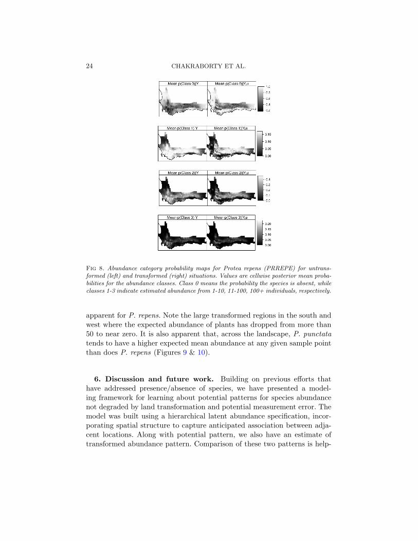
Figures 7 and 8 show the mean posterior abundance category probabili-ties (potential and transformed) for P. punctata (Figure 7) and P. repens(Figure 8). Comparing these plots among rows contrasts the probabilitiesassociated with each abundance class for the species, while comparing be-tween columns shows the effects of landscape transformations on abundanceclass probabilities. Both species show higher predicted abundances coincid-ing with mountainous areas of the CFR. This is where the fynbos biomedominates the landscape and where proteas are characteristically the dom-inant, indicator species (Rebelo et al., 2006). Note that P. punctata, a lesscommon species, is only slightly affected by landscape transformation, whilethere are dramatic differences for P. repens (Figure 9 and 10). This is be-cause P. punctata is mostly limited to dry, rocky or shale slopes (Rebelo,2001) which are less suitable for agriculture or development and thus mostly


Fig 7. Abundance category probability maps for Protea punctata (PRPUNC) for untrans-formed (left) and transformed (right) situations. Values are cellwise posterior mean proba-bilities for the abundance classes. Class 0 means the probability the species is absent, whileclasses 1-3 indicate estimated abundance from 1-10, 11-100, 100+ individuals, respectively.

untransformed. P. repens on the other hand is much more ubiquitous acrossthe region and can frequently occur in lowland areas that have been largelytransformed by human activities (Rebelo, 2001; Rebelo et al., 2006).

It is also useful to summarize these data through mean potential abundanceand mean transformed abundance (see section 4.3) as in Figures 9 and 10.These figures allow inspection of the underlying latent surfaces that areof interest to ecologists as a continuous relative representation of speciesabundances. However, the latent “z” scales may be difficult to interpret eco-logically and thus estimated potential and transformed abundance (usingthe grouped mean) are also shown. These represent the expected abundance(with respect to the p’s or r’s) of a species at a randomly selected samplelocation in that grid. The associated display makes it easy to visualize theeffects of habitat transformation on protea populations. P. punctata showsalmost no effects of landscape transformation, while large differences are


Fig 8. Abundance category probability maps for Protea repens (PRREPE) for untrans-formed (left) and transformed (right) situations. Values are cellwise posterior mean proba-bilities for the abundance classes. Class 0 means the probability the species is absent, whileclasses 1-3 indicate estimated abundance from 1-10, 11-100, 100+ individuals, respectively.

apparent for P. repens. Note the large transformed regions in the south andwest where the expected abundance of plants has dropped from more than50 to near zero. It is also apparent that, across the landscape, P. punctatatends to have a higher expected mean abundance at any given sample pointthan does P. repens (Figures 9 & 10).

6. Discussion and future work. Building on previous efforts thathave addressed presence/absence of species, we have presented a model-ing framework for learning about potential patterns for species abundancenot degraded by land transformation and potential measurement error. Themodel was built using a hierarchical latent abundance specification, incor-porating spatial structure to capture anticipated association between adja-cent locations. Along with potential pattern, we also have an estimate oftransformed abundance pattern. Comparison of these two patterns is help-


Mean z[P] Mean z[T]

−6

−5

−4

−3

−2

−1

0

1

2

Grouped Mean Abundance Grouped Mean Transformed Abundance

0

20

40

60

80

100

120

140

Fig 9. Mean posterior abundance summaries for Protea punctata (PRPUNC). On thelatent z-scale, “Mean z[P]” refers to potential abundance while “Mean z[T]” refers to thepotential abundance corrected for habitat transformation. The Grouped Mean Abundancerescales the Mean z[P] surface to the expected potential size of a population in a gridcell (using the observed abundance classes: absent, 1-10, 10-100, 100+). The Group MeanTransformed Abundance shows the expected size of a population after correcting for habitattransformation.

ful for understanding the effect of land transformation on species presenceand abundance and, in particular, for disentangling these effects from thoseof other environmental factors. This may facilitate designing strategies forspecies conservation as well as understanding the overall effects of climatechange.

This work has applications in biogeography and in conservation biology(Pearce and Ferrier, 2001; Gaston, 2003). We can now develop predictivemaps of “high quality” habitat sites within a species range, based on highpredicted abundances. This will help identify prime locations for effectiveconservation efforts. We can also estimate the impact of habitat transforma-


Mean z[P] Mean z[T]

−2.5

−2.0

−1.5

−1.0

−0.5

0.0

0.5

1.0

Grouped Mean Abundance Grouped Mean Transformed Abundance

0

10

20

30

40

50

60

70

Fig 10. Mean posterior abundance summaries for Protea repens (PRREPE). On the la-tent z-scale, “Mean z[P]” refers to potential abundance while “Mean z[T]” refers to thepotential abundance corrected for habitat transformation. The Grouped Mean Abundancerescales the Mean z[P] surface to the expected potential size of a population in a gridcell (using the observed abundance classes: absent, 1-10, 10-100, 100+). The Group MeanTransformed Abundance shows the expected size of a population after correcting for habitattransformation.

tion on the size of the population using the information from Figure 8 and 10,and thus identify threats to conservation. Predictive abundance maps willalso be useful to explore patterns in biodiversity and species abundances. Dospecies abundances tend to peak in the middle of the species’ range (Gaston,2003) ? Do areas of high biodiversity tend to have lower species abundances? Are there areas that are rich in both abundance and biodiversity (perhapsidentifying ideal regions for conservation efforts) ?

There are several natural extensions. One is to study the temporal change inabundance. With abundance data collected over time as well as associatedenvironmental factors such as rainfall and temperature, dynamic modeling of


species abundance with changing environmental factors, may give a clearerpicture of how a species is responding to climate change. Indeed, when con-nected to future climate scenarios, we may attempt to forecast prospectivespecies abundance. Similarly, if the transformation data is also time varying,we could illuminate the effect of land transformation in greater detail.

The current model uses transformation percentage (1−u) in a deterministicway (transformation having a binary effect on potential abundance). In othercases (e.g., to study abundance pattern of animals) it may be reasonable totreat transformation as another covariate influencing species habitat. Also,it may be imagined that the relationship between potential abundance andenvironmental variables is not linear as specified in (3), e.g., environmentalvariables may affect larger abundance classes differently from smaller abun-dance classes; piecewise linear specification, introducing different regressioncoefficients over the different abundance classes could be explored.

Another possible extension lies in joint modeling of two or more species.One may wish to learn whether two plant varieties are sympatric or al-lopatric and whether or not there is evidence for competitive interactionsor facilitation. Such modeling can be done by extending our model to havemultiple (zP,k, zT,k, zO,k) surfaces, where k is the species indicator. Depen-dence can be introduced in across zP,k surfaces by modeling θ(k) using anMCAR (Gefand and Vounatsou, 2003; Jin et al., 2005). Fitting such modelswill be very challenging if there are many grid cells.

Instead of taking an areal level approach, if covariate information is avail-able at point level (where sampling sites are viewed as “points” within thelarge region, D), one may consider a point-level model. This amounts to re-placing the CAR model with a Gaussian process prior for the spatial effects.With many sampling sites, we will need to use appropriate approximationtechniques (Banerjee et al., 2008).

Acknowledgement. The authors thank Guy Midgley and Anthony Re-belo for useful discussions.

APPENDIX A

A.1. Proof of E(zT ) finite.

Proof. E(zT ) = E(E(zT |zP )) = E(uzP + (1 − u)c(zP )) = E(zP − (1 −u) φ(zP )

1−Φ(zP )). Assuming zP ∼ N(µ, 1), enough to show∫ ∞−∞

φ(x)1−Φ(x))φ(x −


µ) dx < ∞Consider the quantity x2 φ(x)

1−Φ(x))φ(x − µ), if x → −∞, it goes to 0. Whenx → ∞, we have

limx→∞

x2 φ(x)

1 − Φ(x))φ(x − µ)

L′ptal= lim

x→∞

2xφ(x)φ(x − µ) − x3φ(x)φ(x − µ) − x2(x − µ)φ(x)φ(x − µ)

−φ(x)

= 0

So lim|x|→∞ x2 φ(x)1−Φ(x))φ(x − µ) = 0, thus we can get B1 < 0, B2 > 0, such

that φ(x)1−Φ(x))φ(x−µ) < 1

x2 for all x /∈ (B1, B2). Hence the result follows.

A.2. Posterior simulation of z’s for a site with no presence ob-served. We subdivide by considering the ways that we can generate a 0realization of y based on Eq. (3.5) (one may also use Eq. (3.3) to do this).

(i) The area is untransformed, the species was potentially there, butmissed during data collection or it was absent at that time instance; theevent is 1zP≥α0,zO≤α0 with prior probability π1 = uP (zP ≥ α0, zO ≤α0)

(ii) Potentially the species was absent there; the event is 1zP≤α0 with priorprobability π2 = P (zP ≤ α0)

(iii) The species was potentially there 1zP≥α0 , but the area was trans-formed; the event has prior probability π3 = (1 − u)P (zP ≥ α0).

These three events are exhaustive and mutually exclusive for the event(y = 0). Thus f(zP , zO|y = 0,Θ) is a 3-component mixture. To draw a(zP , zO) pair from this distribution amounts to first choosing a componentand then drawing a pair (zP , zO) from that component distribution. ByBayes rule, conditional on observed (y = 0), these three cases can happen

with posterior probability πi/3

∑

l=1

πl, i = 1, 2, 3. So we use a multinomial

to select which of these events took place. Before going into case by casedetails, it is worth mentioning that, in all these cases the sampling fromthe joint density of chosen mixture component was done via the marginalf(zP | · ·) followed by f(zO|zP , ··). The advantage of this scheme is that wedon’t need to draw from the latter because zO’s corresponding to y = 0 arenot involved in posterior full conditionals of any other parameters in themodel (as α0 = 0, fixed). If the second case is selected then f(zO, zP |·, ·) ∝[

uδzP+ (1 − u)δc(zP )

]

1zO≤01zP≤0φ(zP ) and thus marginalizing over zO, we


get f(zP | · ·) ∝ φ(zP )1zP≤0 which is a truncated Gaussian on R−. Simi-

larly under case (iii), we need to simulate zP from φ(zP )1zP≥0, a Gaussiantruncated on R

+. In case (i), f(zO, zP |·, ·) ∝ φ(zO; zP , 1)1zP≥01zO≤0φ(zP ),so marginalizing over zO we get f(zP | · ·) ∝ φ(zP )(1 − Φ(zP ))1zP≥0. An ef-ficient way to draw from this density is to propose a zP from a truncatednormal on R

+ and do a Metropolis-Hastings update with an independentproposal, using the quantity (1 − Φ(·)). However all sampling distributionsare summarized in A.3 below.

A.3. Posterior full conditionals needed for Gibbs sampling.

• If yij > 0, draw zO,ij N(zP,ij , 1)1(αyij−1,αyij). Draw zP,ij ∼ N(

vTi

β+θi

2 +zO,ij

2 , 12)

• If yij = 0, compute pij = (uΦ2([0,∞]× [−∞, 0] ; µij ,Σ0), 1−Φ(vTi β +

θ), (1−u)Φ(vTi β+θi)), where µij = (vT

i β+θi, vTi β+θi) and Σ0 =

(

1 11 2

)

are the location and dispersion parameters for bivariate normal joint

prior distribution of (zO,ij , zP,ij). Draw diji.i.d.∼ mult(pij). If dij = 1,

propose zproposeP,ij ∼ N(vT

i β + θi, 1)1(0,∞) and do a Metropolis Hast-

ings sampler using (1 − Φ(·)). Else if dij = 2 draw zP,ij ∼ N(vTi β +

θi, 1)1(−∞,0), else draw zP,ij ∼ N(vTi β + θi, 1)1(0,∞)

• Draw αh = unif(maxij:yij=h zO,ij ,minij:yij=h+1 zO,ij), h = 1, 2• Draw β ∼ N(µβ,Σβ)

∏

i,j N(zP,ij ; vi, β, θi)

• Draw θi ∼ N(zP,ij ; vi, β, θi)N(

∑

jwijθj

wi+,

τ20

wi+) for i = 1, 2, ...,m. Draw

θi ∼ N(

∑

jwijθj

wi+,

τ20

wi+) for i = m + 1, 2, ..., I

REFERENCES

Albert, J.H. and Chib, S. (1993) Bayesian analysis of binary and polychotomous re-sponse data. Journal of the American Statistical Association 88: 670–679.

Armstrong, M., Galli, A.G., Le Loc’h, G., Geffroy, F. and Eschard R. (2003)Plurigaussian simulations in geosciences. Springer-Verlag, Berlin, Germany.

Banerjee, S., Gelfand, A.E., Finley, A.O. and Sang, H. (2008) Gaussian predictiveprocess models for large spatial datasets. Journal of the Royal Statistical Society, SeriesB 70: 825–848.

Banerjee S., Carlin, B.P. and Gelfand, A.E. (2004) Hierarchical modeling and anal-ysis for spatial data. Chapman and Hall/CRC, Boca Raton

Beale, C. M., Lennon, J. J., Elston, D. A., Brewer, M. J. and Yearsley, J. M.

(2007) Red herrings remain in geographical ecology: a reply to Hawkins et al. Ecography30: 845–847.

Besag, J. (1974) Spatial interaction and the statistical analysis of lattice systems (withdiscussion). Journal of the Royal Statistical Society, Series. B 36: 192–236.


Besag, J. and Kooperberg, C. (1995) On conditional and intrinsic autoregressions,Biometrika 82(4): 733–746.

Busby, J. R. (1991) BIOCLIM A bioclimatic analysis and predictive system. In : NatureConservation: Cost Effective Biological Surveys and Data Analysis (Eds. C.R. Margulesand M.P. Austin.) pp. 64–68. CSIRO: Canberra.

Conroy, M.J., Runge, J.P., Barker, R.J., Schofield, M.R. and Fonnesbeck, C.J.

(2008) Efficient estimation of abundance for patchily distributed populations via two-phase, adaptive sampling. Ecology 89: 3362–3370.

Cressie, N., Calder, C.A., Clark, J.S., Ver Hoef, J.M. and Wikle, C.K. (2009)Accounting for uncertainty in ecological analysis: the strengths and limitations of hier-archical statistical modeling. Ecological Applications 19(3): 553–570.

De Oliveira, V. (2000) Bayesian prediction of clipped Gaussian random fields. Compu-tational Statistics and Data Analysis 34: 299–314.

Diggle, P.J., Menezes, R. and Su, T-L. (2010) Geostatistical analysis under preferen-tial sampling (with Discussion). Journal of the Royal Statistical Society, Series. C (toappear).

Elith, J., Graham, C. H., Anderson, R. P., Dudık, M., Ferrier, S., Guisan, A., Hi-

jmans, R. J., Huettmann, F., Leathwick, J. R., Lehmann, A., Li, J., Lohmann,

L. G., Loiselle, B. A., Manion, G., Moritz, C., Nakamura, M., Nakazawa,

Y., Overton, J. McC., Peterson, A. T., Phillips, S. J., Richardson, K. S.,

Scachetti-Pereira, R., Schapire, R. E., Soberon, J., Williams, S., Wisz, M.

S. and Zimmermann, N. E. (2006) Novel methods improve prediction of species’ dis-tributions from occurrence data. Ecography 29: 129–151.

Fitzpatrick, M.C., Gove, A.D., Nathan J. Sanders, N.J. and Dunn, R.R. (2008)Climate change, plant migration, and range collapse in a global biodiversity hotspot: theBanksia (Proteaceae) of Western Australia. Global Change Biology 14(6): 1337-1352.

Fuller, W.A. (1987) Measurement Error Models. John Wiley & Sons, Inc., New York.Gaston, K. (2003) The structure and dynamics of geographic ranges. 1st edition. Oxford

University Press, Oxford.Gelfand, A. E., Silander, J. A. Jr., Wu, S., Latimer, A. M., Lewis, P., Rebelo,

A.G. and Holder, M. (2005) Explaining species distribution patterns through hier-archical modeling. Bayesian Analysis 1: 42–92.

Gelfand, A.E., Schmidt, A. M., Wu, S., Silander, J. A. Jr., Latimer, A. M. and

Rebelo, A.G. (2005) Modelling species diversity through species level hierarchicalmodeling. Journal of the Royal Statistical Society, Series C 54(1): 1–20.

Gelfand, A.E. and Vounatsou, P. (2003) Proper multivariate conditional autoregres-sive models for spatial data analysis. Biostatistics 4: 11–25.

Gelfand, A. E. and Sahu, S. K. (1999) Identifiability, improper priors, and Gibbssampling for generalized linear models. Journal of the American Statistical Association94: 247–253.

Goldblatt, P. and Manning, J. (2000) Cape plants: a conspectus of the Cape Flora ofSouth Africa. National Botanical Institute of South Africa, Cape Town

Gorresen, P.M., McMillan, G.P., Camp, R.J. and Pratt, T.K. (2009) A spatialmodel of bird abundance as adjusted for detection probability. Ecography 32: 291–298.

Graham, C.H. and Hijmans, R.J. (2006) A comparison of methods for mapping speciesranges and species richness. Global Ecology and Biogeography 15: 578–587.

Guisan, A. and Zimmerman, N. E. (2000) Predictive Habitat Distribution Models inEcology. Ecological Modelling 135: 147–186.

Guisan, A. and Thuiller, W. (2005) Predicting species distribution: offering more thansimple habitat models. Ecology Letters 8: 993–1009.


Guisan, A., Lehman, A., Ferrier, S., Austin, M.P., Overton, J.M.C., Aspinall,

R. and Hastie, T. (2006) Making better biogeographical predictions of species’ dis-tributions. Journal of Applied Ecology 43: 386–392.

Higgs, M.D. and Hoeting, J.A. (2009) A clipped latent-variable model for spatiallycorrelated ordered categorical data. In Review.

Hooten, M.B., Larsen, D.R. and Wikle, C.K. (2003) Predicting the spatial distribu-tion of ground flora on large domains using a hierarchical Bayesian model. LandscapeEcology 18: 487–502.

Ibanez, I., Silander, J.A. Jr., Allen, J.M., Treanor S. and Wilson, A. (2009)Identifying hotspots for plant invasions and forecasting focal points of further spread.Journal of Applied Ecology (in review)

Jin, X., Carlin, B.P. and Banerjee, S. (2005) Generalized hierarchical multivariateCAR models for areal data. Biometrics 61: 950-961.

Kunin, W.E., Hartley, S. and Lennon, J. (2000) Scaling down: On the challenges ofestimating abundance from occurrence patterns. The American Naturalist 156: 560-566.

Latimer, A. M., Wu, S., Gelfand, A.E. and Silander, J. A. Jr. (2006) Buildingstatistical models to analyze species distributions. Ecological Applications 16(1): 33–50.

Le Loc’h, G. and Galli, A. (1997) Truncated plurigaussian method: Theoretical andpractical points of view. In: E.Y. Baafi and N.A. Schofield (eds.) Geostatistics Wollon-gong ’96, Vol. 1: 211–222.

Loarie, S.R., Carter, B.E., Hayhoe, K., McMahon, S., Moe, R., Knight, C.A.,

and Ackerly, D.D. (2008) Climate change and the future of California’s endemicflora. PLoS ONE 3: e2502.

Mallick, B. and Gelfand, A.E. (1995) Bayesian analysis of semiparametric propor-tional hazards models. Biometrics 51: 843–852.

Midgley G.F. and Thuiller, W. (2007). Potential vulnerability of Namaqualand plantdiversity to anthropogenic climate change. Journal of Arid Environments 70: 615–628.

Mueller-Dombois, D. and Ellenberg, H. (2003) Aims and methods of vegetationecology. Blackburn Press, Caldwell, NJ.

Pearce, J and Ferrier, S. (2001) The practical value of modelling relative abundance ofspecies for regional conservation planning: a case study. Biological Conservation 98(1):33–43

Phillips, S. J. and Dudık, M. (2008) Modeling of species distributions with Maxent:new extensions and a comprehensive evaluation. Ecography 31: 161–175.

Potts, J. M. and Elith, J. (2006) Comparing species abundance models. EcologicalModelling 199(2): 153–163.

Pressey, R.L., Cabeza, M., Watts, M.E. Cowling, R.M. and Wilson, K.A. (2007)Conservation planning in a changing world. Trends in Ecology and Evolution 22: 583–592.

Raxworthy, C.J., Martinez-Meyer, E., Horning, N., Nussbaum, R.A., Schneider,

G.E., Ortega-Huerta, M.A. and Peterson, A.T. (2003) Predicting distributionsof known and unknown reptile species in madagascar. Nature 426: 837–841.

Rebelo, A. G. (1991) Protea Atlas Manual: instruction booklet to the protea atlasproject. Protea Atlas Project Cape Town.

Rebelo, A. G. (2001) Proteas: a field guide to the proteas of southern Africa. FernwoodPress Vlaeberg, South Africa (2nd Edition).

Rebelo, A. G. (2002) The state of plants in the Cape Flora. In Proceedings of a conferenceheld at the Rosebank Hotel in Johannesburg 18: (Eds: G.H. Verdoorn and J. Le Roux)The State of South Africa’s Species. Endangered Wildlife Trust.


Rebelo, A. G. (2006) Protea atlas project website.http://protea.worldonline.co.za/default.htm

Rebelo, A. G., C. Boucher, N. Helme, L. Mucina and Rutherford, M. C. (2006)Fynbos Biome. In: L. Micina and M.C. Rutherford (eds.) The Vegetation of SouthAfrica, Lesotho and Swaziland. Streltzia 19. South African National Biodiversity Insti-tute, Pretoria, South Africa.

Rouget, M., Richardson, D. M., Cowling, R. M., Lloyd, J. W., and Lombard,

A. T. (2003) Current patterns of habitat transformation and future threats to biodi-versity in terrestrial ecosystems of the Cape Floristic Region, South Africa. BiologicalConservation 112: 63–83.

Royle, J.A., Kery, M., Gautier, R. and Schmidt, H. (2007). Hierarchical spatialmodels of abundance and occurrence from imperfect survey data. Ecological Monographs77: 465–481.

Royle, J.A., and Link, W.A. (2006) Generalized site occupancy models allowing forfalse positive and false negative errors. Ecology 87(4): 835–841.

Schwartz, M.W., Iverson, L.R., Prasad, A.M., Matthews, S.N. and O’Connor,

R.J. (2006) Predicting extinctions as a result of climate change. Ecology 87(7): 1611–1615.

Stefanski, L.A. and Carroll, R.J. (1987) Conditional scores and optimal scores forgeneralized linear measurement-error models. Biometrika 74: 703–716.

Sutherland, W.J. (2006) Ecological census techniques. 2nd edition. Cambridge Univer-sity Press. Cambridge.

Ver Hoef, J.M., Cressie, N., Fisher, R.N. and Case, T.J. (2001) Uncertainty andspatial linear models for ecological data. In: Spatial Uncertainty in Ecology (eds. Hun-saker, C.T., Goodchild, M.F., Friedl, M.A. and Case, T.J.), 214–237. Springer Verlag,New York.

Ver Hoef, J. M., and Frost, K. (2003) A Bayesian hierarchical model for monitoringharbor seal changes in Prince William Sound, Alaska. Environmental and EcologicalStatistics 10: 201–209.

Wisz, M.S., Hijmans, R.J., Li, J., Peterson, A.T., Graham, C.H. and Guisan,

A. (2008) Effects of sample size on the performance of species distribution models.Diversity and Distributions 14: 763–773.

Avishek Chakraborty

Alan E. Gelfand

Department of Statistical Science

Duke University

Durham, NC 27708

U.S.A.

E-mail: [email protected]@stat.duke.edu

Adam M. Wilson

John A. Silander, Jr.

Department of Ecology and Evolutionary Biology

University of Connecticut

Storrs, CT 06269

U.S.A.

E-mail: [email protected]@uconn.edu

Andrew M. Latimer

Department of Plant Sciences

University of California

Davis, CA 95616

U.S.A.

E-mail: [email protected]

http://protea.worldonline.co.za/default.htm

mailto:[email protected]





MODELING LARGE SCALE SPECIES ABUNDANCE …ac103/abundance_aoas.pdfSubmitted to the Annals of Applied...

Documents

Transcript of MODELING LARGE SCALE SPECIES ABUNDANCE …ac103/abundance_aoas.pdfSubmitted to the Annals of Applied...