
MODELING LAPSE RATES Investigating the Variables...
78
MODELING LAPSE RATES 1 Faculty of Management and Governance Department of Finance and Accounting Financial Engineering and Management MODELING LAPSE RATES Investigating the Variables that Drive Lapse Rates December 08, 2011 Zeist, the Netherlands Master Thesis Author: Cas Z. Michorius Committee: Dr. ir. E.A. van Doorn (University of Twente) Dr. B. Roorda (University of Twente) Drs. P.J. Meister AAG (Achmea)
-
Upload
phungkhanh -
Category
Documents
-
view
216 -
download
0
Transcript of MODELING LAPSE RATES Investigating the Variables...
MODELING LAPSE RATES 1
Faculty of Management and Governance
Department of Finance and Accounting
Financial Engineering and Management
MODELING LAPSE RATES
Investigating the Variables that
Drive Lapse Rates
December 08, 2011
Zeist, the Netherlands
Master Thesis
Author: Cas Z. Michorius
Committee: Dr. ir. E.A. van Doorn (University of Twente)
Dr. B. Roorda (University of Twente)
Drs. P.J. Meister AAG (Achmea)

MODELING LAPSE RATES 2
MODELING LAPSE RATES 3
MASTER THESIS
Modeling Lapse Rates:
Investigating the Variables That Drive Lapse Rates
December 08, 2011
Zeist, the Netherlands
Author: Cas Z. Michorius
Project initiator: Achmea holding, Zeist

MODELING LAPSE RATES 4
Abstract
In the life insurance industry individually closed contracts are accompanied by risks. This
report focuses on one of these risks, more specifically, the risk involving the termination of
policies by the policyholders or, as it is called, “lapse” risk
The possibility of a lapse can influence the prices of contracts, necessary liquidity of an
insurer and the regulatory capital which should be preserved. The possibility of a lapse is
reckoned to account for up to 50% of the contract‟s fair value and one of the largest
components of the regulatory capital. For these reasons it is of great importance to
prognosticate lapse rates accurately. These were the main reasons for conducting this research
on behalf of Achmea and for investigating models and explanatory variables. The research
question which functioned as the guide line for this research at Achmea is the following:
Can the current calculation model for lapse rates be improved1, while staying in compliance
with the Solvency II directive, and which variables have a significant2 relation to the lapse
rates?
The model applied and the explanatory variables analyzed are the result of a literature study.
This study provided the Generalized Linear Model [GLM] to be a suitable choice and led to a
list of 38 possible explanatory variables of which 9 were tested 3
. The GLM was applied to the
data of CBA and FBTO corresponding to the years 1996 to 2010 and aggregated per product
group. The seven product groups that were analyzed were: mortgages, risk, savings (regular
premium), savings (Single premium), unit-linked (Regular premium), unit-linked (Single
premium) and whole life & funeral. The aggregation of the data has been done using Data
Conversion System and Glean, two products of Sungard, and the data were analyzed using
SPSS 17, a product of IBM.
The research provided seven models, one for each product group, including variables as
“buyer confidence”, “first difference in lapse rates”, “gross domestic product [GDP]”,
“inflation”, “reference market rate” and “return on stock market”. Every model provided more
accurate predictions than the application of the mean of the data would. It should be noted
1 The performance of the model has been measured in terms of accuracy, on which it has also been compared.
2 The significance of the variables has been tested by statistical measures using a 5% level of significance.
3 Lagged values of these variables have been included as well, which led to a total of 14 analyzed variables.
MODELING LAPSE RATES 5
that, due to lack of data, this comparison has been done on the training set. The performance
of the models, when compared with the model provided by regulatory bodies (standard
formula), is dependent on the level of expected lapse rates as well as the relative error of the
predicted values. The level of the expected lapse rates greatly influences the standard formula,
whereas the relative error of the predicted values is one of the great contributors to the
prediction interval of the developed model.
Additional research showed that the choice for division of the data into several product groups
is supported by the huge diversity in lapse rate developments amongst the product groups.
Further analysis of the lapse rates with respect to the duration of policies also provided a
reason for further research. The analysis indicated that the effect of macro-economic variables
on lapse rates is dependent on its duration, indicating that the data per product group can be
subdivided or duration can be used as explanatory variable.
Based on the research results it is recommended to analyze the possibility of generalizing the
results by extending the research to other parts of Achmea. Next to that, it is recommended to
investigate the data on a policy level in order to assess the significance of other variables.
These additional researches will also increase the statistical strength and accuracy of the
inferences that can be made. It is also recommended to clarify the importance of (accurate
recording of) lapse rates and to denote a universal definition of a lapse, all to make sure that
the lapse data become unpolluted. Finally, it is advised to monitor the models and to examine
their performance and sensitivity to new data.

MODELING LAPSE RATES 6
Preface
Six years ago I commenced studying mechanical engineering, a bachelor study, at Saxion
University of Applied Sciences. After graduation I chose to enroll for the master‟s study
Financial Engineering and Management at the University of Twente to learn to apply my
mathematical skills to problems which are more financial by nature. During this master I
studied several courses which were (partly) focused on the insurance industry. These courses
raised my curiosity for the actual insurance industry and led to the application at Group Risk
Management of Achmea.
During the internship at Achmea I received help from several colleagues. Of these I would
like to thank L. Menger for interesting me in the research topic, providing much relevant
information and his guidance during the first weeks. For subsequent guidance and the final
review of this report I would like to thank P. J. Meister and T. Delen. Naturally I am thankful
for the opportunity to graduate at Achmea for which I have to thank M.R. Sandford. I would
like to thank all other colleagues at Group Risk Management and Actuarial Reporting who
provided time and information, of which special thanks goes out to R.A. Schrakamp for
providing the research data.
From the University of Twente I would like to thank E.A. van Doorn for being prepared to act
as my supervisor throughout this period and for his remarks and suggestions which have
helped me to improve this thesis. Also from the University Of Twente is B. Roorda who I
would like to thank for being prepared to act as additional/second supervisor and for his
answers to difficult questions throughout my master‟s program.
Finally, I would like to thank S.A. Leferink and Y.F.M. Michorius for their support and all
their additional comments without which this thesis could not have been finalized.

MODELING LAPSE RATES 7
TABLE OF CONTENTS
LIST OF IMPORTANT DEFINITIONS 9
CHAPTER 1 INTRODUCTION 11
CHAPTER 2 LAPSE RATES 14
2.1 THE RISE OF THE LIFE- AND PENSIONS INDUSTRY 14
2.2 THE RISKS WHICH ARE ASSOCIATED WITH THE LIFE- AND PENSIONS INDUSTRY 15
2.3 THE INTENTION OF SOLVENCY I AND II 16
2.4 SOLVENCY II 17
2.5 LAPSE RISK 18
2.6 LAPSE EVENTS 19
2.7 LAPSE EVENTS AND SOLVENCY II 20
CHAPTER 3 EXPLANATORY VARIABLES 22
3.1 EXPLANATORY VARIABLES IN LITERATURE 22
3.2 POSSIBLE EXPLANATORY VARIABLES 25
CHAPTER 4 PREDICTIVE MODELS 27
4.1 PREDICTIVE MODELS 27
4.2 THE REQUIREMENTS OF REGULATORY BODIES (THE DNB) FOR THE LAPSE RATE MODEL 29
4.3 ACHMEA’S INTERNAL MODEL 30
4.4 GENERALIZED LINEAR MODELS 32
4.5 THE LINK FUNCTION 34
CHAPTER 5 METHODS 37
5.1 SCOPE OF THE RESEARCH 37
5.2 APPARATUS 37
5.3 PROCEDURE & MEASUREMENT 38
5.3.1 Conditions which can be checked before formation of a model. 39
5.3.2 Model formation. 41
5.3.3 Condition which can be checked after formation of a model. 43
5.3.4 Selection of a model. 44
5.3.5 Conditions which can be checked after selection of the model. 45
5.3.6 Product groups for which models are formed. 46
5.3.7 Additional research. 48
5.4 (POSSIBLE) LIMITATIONS 48

MODELING LAPSE RATES 8
CHAPTER 6 DATA AND ANALYSIS 49
6.1 DATA SET 49
6.2 ANALYSIS 50
6.2.1 Formation of the model. 51
6.2.2 Comparison of the developed with the standard model. 61
6.2.3 Results of the other product groups. 63
6.2.4 Results of the additional research. 64
6.3 LIMITATIONS 66
CHAPTER 7 CONCLUSION AND RECOMMENDATION 67
7.1 CONCLUSION 67
7.2 RECOMMENDATION 69
REFERENCES 70
APPENDICES 77
APPENDIX 1: RISK MAP 78

MODELING LAPSE RATES 9
List of Important Definitions
The following definitions are those of terms which are used throughout this document.
An internal model is a model developed by an insurer to (partly) replace the Solvency II
standard model.
A lapse (event) is the termination of coverage by the policy owner/insured.
Note: In this study a “lapse event” is said to occur if a personal contract is fully terminated by
the policy holder and non-revivable, regardless of the refund, administrated at a divisional
level.
The lapse rate of a particular product group in a particular time period is the fraction of
lapses of the product group in that time period.
Lapse risk is the risk of loss, or of adverse change in the value of insurance liabilities,
resulting from changes in the level or volatility of the rates of policy lapses, terminations,
renewals and surrenders.
The Minimum Capital Requirement (MCR) “is the minimum level of security below which
the amount of financial resources should not fall. When the amount of eligible basic own
funds falls below the Minimum Capital Requirement, the authorisation of insurance and
reinsurance undertakings should be withdrawn.”(Solvency II Association, n.d.a)
The outcome/response variable is a dependent variable whose value is typically determined
by the result of a set of independent and random variables.
The predictor/explanatory variable is an “independent” variable which is used to explain or
predict the value of another variable.
The risk-free rate (of return) is the best rate that does not involve taking a risk. Both the
return of the original capital and the payment of interest are completely certain. The risk free
rate for a given period is taken to be the return on government bonds over the period. This is
because a government cannot run out of its own currency, as it is able to create more than
necessary.
MODELING LAPSE RATES 10
Solvency 2 “is a fundamental review of the capital adequacy regime for the European
insurance industry. It aims to establish a revised set of EU-wide capital requirements and risk
management standards that will replace the current solvency requirements.” (Solvency II,
Financial Services Authority).
The Solvency Capital Requirement (SCR) “should reflect a level of eligible own funds that
enables insurance and reinsurance undertakings to absorb significant losses and that gives
reasonable assurance to policyholders and beneficiaries that payments will be made as they
fall due” (Solvency II Association, n.d.b) to ensure that an (re)insurance company will be able
to meet its obligations over the next 12 months with a probability of at least 99.5%.
The standard model is the model prescribed by the Solvency II directive.
A surrender is a terminated policy, like a lapse, but when there is still a cash refund.
A termination is the cancellation of a life insurance policy by either the policyholder or the
insurance company.

MODELING LAPSE RATES 11
Chapter 1 Introduction
In the life insurance industry individually closed contracts are accompanied by risks. This
report focuses on one of these risks, specifically the risk of termination of a policy by the
policyholder.
Policyholders may exercise their right to terminate a contract; this event is called a lapse. One
of the problems with policies that lapse (at an early stage) is that not enough premium
payments have been made to cover the policy expenses. To diminish the negative effects of a
lapse, the loss on lapsed contracts is included in the calculation of new policy prices.
Consequently present and future policyholders will be held accountable for this risk by
adjusting future premiums. According to Grosen & Jorgensen (2000) the option to lapse can,
under certain conditions, account for up to 50% of the contract‟s fair value.
The uncertainty that surrounds policy lapses is the source of yet other problems. This
uncertainty or risk of loss due to the level and volatility of lapses is called lapse risk. To
ensure an insurer‟s continuity certain required buffers, or regulatory capital, are specified by
regulatory bodies. This regulatory capital should be preserved in a manner which is
considered to be risk free. Figures from Achmea (2010b) indicate that the increase in lapse
risk during 2010 accounted for the largest increase in regulatory capital. In order to mitigate
the negative effects of policy lapses it is important for an insurance company to develop
reliable models for predicting lapse rates. The recorded study on lapse rates goes back to the
beginning of the 20th century, where Papps (1919) tried to forecast lapse rates using an
analytical formula. Soon afterwards theories were developed on the influences of variables on
future lapse rates. Well-known hypotheses are the interest rate hypothesis and the emergency
fund hypothesis. The interest rate hypothesis suspects interest rate to be an explanatory
variable of lapse rates. It bases that suspicion on the thought that a change in relative
profitability of alternative investments might arise from interest rate fluctuation. This
hypothesis presumes that the market interest rate is seen as opportunity cost (Kuo, Tsai &
Chen, 2003). Looking at insurances from a different angle the emergency fund hypothesis
suggests that an insurance is seen “as an emergency fund to be drawn upon in times of
personal financial crisis” (Outreville, 1990, p.249). Although many of the past studies focused
on these hypotheses, recent research shifted to more complex predictors of lapse rates. The
huge diversity in published researches demonstrates that characteristics or behavior of the
MODELING LAPSE RATES 12
policyholder, insurance company and macro-economic environment can all experience a
significant association with lapse rates.
Associated with the research on explanatory variables is the research on predictive modeling,
in which explanatory variables can be included. Outreville (1990) published an article on
predicting lapse rates by use of explanatory variables which stirred up the interest in and
modeling of lapse rates. The number of publications on predictive models increased rapidly
since then, covering a vast amount of models ranging from single- to multi-factor models.
Even though many years of research have been conducted since then, no consensus has been
established on the specific model which should be used. Publishing authors concur that it is
due to the large variety of conditions per study that the insurance industry lacks a universally
applicable model and universally significant drivers. Studies on models which are done by
Kim (2005 and 2009) show that the choice for a model is, both, case as well as requirement
dependent.
For Achmea it is necessary to determine a predicted value of the lapse rates for calculations,
such as the pricing of insurances, and forecasting of cash flows. The goal of this research is to
find those variables which are seen as significant drivers of lapse rates and to determine which
model is most fit for forecasting with those variables. The model is subjected to requirements
set by regulatory bodies as well as company specific requirements. The regulatory body, in
this case De Nederlandsche Bank [DNB], employs the Solvency II which is developed by the
European Insurance and Occupational Pensions Authority [EIOPA4] to improve the
supervision of European insurers.
Summarizing, this research should comply with the requirements/legislation and has been
conducted to provide an answer to the question:
Can the current calculation model for lapse rates be improved5, while staying in compliance
with the Solvency II directive, and in particular, which variables have a significant 6relation to
the lapse rates?
4 EIOPA is one of three European Supervisory Authorities and is an independent advisory body to the European
Parliament and the Council of the European Union.
5 The performance of the model will be measured in terms of accuracy, on which it will also be compared.
6 The significance of the variables will be tested by a well-chosen statistical measure and should render a not yet
specified level of significance.
MODELING LAPSE RATES 13
To answer this question a literature study has been conducted on Solvency II, lapse risk and
lapse rates. Subsequent study has been done to provide a set of variables which were expected
to have significant influence on the lapse rate. A similar comparison study has been
performed for predictive models. Finally, using selection criteria and statistical methods, a
model has been formed. The performance of the model is analyzed by comparing the model
with the current lapse rate prediction method and a prediction method which is in
development.
This thesis is organized as follows.
Chapter two, lapse rates, starts with the rise of the life- and pension business as an
introduction and provides an overview of the regulations and associated risk
categories. Subsequently, the relationship between the regulations, risks and this
research will be provided, which is done by illustrating the importance of lapse rates.
Chapter three, explanatory variables, provides an overview of various insights and
expectations on lapse rates which have been tested in literature. The chapter ends with
a table in which all variables which have proven to experience or are expected to
experience a significant relationship with lapse rates are listed.
Chapter four, predictive models, provides an overview of the various types of models
which are widely used in the life insurance industry. Model requirements as well as
the results of researches which have been conducted internally are presented in this
chapter. The chapter concludes with different recommended approaches dependent on
the type of data which will be analyzed.
Chapter five, methods, briefly covers the scope of the research, used tools, analysis
procedure and (possible) limitations.
Chapter six, data and analysis, provides information on the sources which constitute
the used data set. The chapter continuous with a description of the data analysis and
the obtained results for all product groups and of additional research.
Chapter seven, conclusion and recommendation, provides some concluding remarks
and recommendations for improvements.
At the end of this thesis, after chapter seven, the list of literature sources and
appendices can be found.
MODELING LAPSE RATES 14
Chapter 2 Lapse Rates
In this chapter the concept lapse rate is elaborated and consequently the influence of a single
lapse will be elaborated as well. To understand the influence that lapse rate have on the
insurer this chapter provides a top-down elaboration of the risks accompanying an insurance
agency. After it is indicated which risk categories are existent and into which category the
lapse rates belong. Subsequently the operational definition of a “lapse event” is stated and the
relations between lapses, regulations and costs are mentioned, which led to the research
question.
2.1 The Rise of the Life- and Pensions Industry
In literature many stories are told about the rise of insurance industries all around the globe.
Regardless of the origin of the insurance scheme, which could be in India (Smith, 2004) or in
Rome (Robinson, 2009), they all served a similar purpose, namely; to hedge against the risk
of a contingent, uncertain loss at the expense of a certain but relatively small loss in the form
of a payment.
Through history many groups came up with a scheme to minimize exposure to a specific risk,
like the loss of cargo at sea, by forming a “club”. Members of such a club would pay a
premium at a specified frequency, of which the amount depended on factors as the coverage
length and the desired type of insurance. One of the more popular insurance clubs was the
burial club (Davis, 2006). Membership of a burial club ensured that the funeral expenses of
the person insured would be covered. Even though these clubs existed for centuries it took the
insurance industry a long time before the first legal privately owned insurer was founded.
Based on similar thoughts as the stories of the ancient sailors and burial clubs Achmea‟s story
started. It was in 1811 that a group of 39 Frisian farmers formed an insurance company called
Achlum, to insure their possessions against fire (Achmea, 2010a). This group of farmers grew
and merged with many other groups which all had their own founding story. The merger of
many of such companies led to the present conglomerate which provides insurances and
pensions as well as banking services. At the moment Achmea is the largest life insurer in the
Netherlands and has based its operations within as well as across the Dutch border. Achmea
employs around 22.000 employees and has a total of approximately 5 million policies
MODELING LAPSE RATES 15
outstanding (Nederlandse Zorgautoriteit, 2011). The vast amount of policies in the product
mix of Achmea may range from those that guarantee death benefits to retirement plans.
2.2 The Risks Which Are Associated with the Life- and Pensions Industry
The predecessors of present day insurers soon discovered that their simple insurance schemes
exposed them to many risks. Some of the people that recognized the flaws in insurances
would try to exploit them. Low to no entrance requirements was one of those flaws and led to
adverse selection (Lester, 1866). People, aware of a child‟s bad condition and low life
expectancy, would enroll the child in more than one club knowing that only a few premium
payments would provide a large death benefit. Such flaws in insurances led to the bankruptcy
of many insurers. As time went by, most of these risks have been dealt with due to the
evolution of the insurance industry and its products. The present life- and pensions business
recognizes the following risk categories7:
Life underwriting risk, also referred to as technical insurance risk, is the risk of a
change in (shareholders’) value due to a deviation of the actual claims payments from
the expected amount of claims payments (including expenses).
Note: Life underwriting risk, like all the other risks, can be sub-divided into many risk
types. One of the seven risks into which life underwriting risk can be divided is lapse
risk. The seven underlying risks and especially lapse risk will be elaborated later on.
The financial risks; Premiums that are paid by the insured are invested in financial
assets backing the insurance liabilities. Just as underwriting risk, financial risks are
very material for insurance companies. Financial risks can be categorized into the
following risks:
Market risk is the risk of changes in values caused by market prices or
volatilities of market prices differing from their expected values.
Credit risk is the risk of a change in value due to actual credit losses deviating
from expected credit losses due to the failure to meet contractual debt
obligations.
Liquidity risk is the risk stemming from the lack of marketability of an
investment that cannot be bought or sold quickly enough to prevent or
minimize a loss.
7 All definitions are derived from the Solvency II glossary (Comité Européen des Assurances, 2007).
MODELING LAPSE RATES 16
Operational risk is the risk of a change in value caused by the fact that actual losses,
incurred for inadequate or failed internal processes, people and systems, or from
external events (including legal risk), differ from the expected losses.
A graphical representation of these risks is presented in appendix 1 “Risk map”.
2.3 The Intention of Solvency I and II
Solvency I is the first legislation for (re)insurance companies in the European Union that
addressed rules on solvability requirements. It was introduced in the early 1970‟s by the
European Commission (Cox & Lin, 2006). The Solvency regulation compelled the
(re)insurers within their jurisdiction to hold an amount of capital as a reserve in case an
extreme event should occur.
A lot has changed since 1970. Risks have altered and become more diverse, the products have
become more complex and more and more businesses have expanded their activities across
their national border. This increase in complexity of the insurance industry is the reason why
Solvency II has been developed.
Where Solvency I concentrated on insurance liabilities and sum at risk, Solvency II includes
investment, financing and operational risk for the calculation of the capital requirement. This
expansion provides a more risk-based measure. Apart from a better quantification of the risks,
the regulation provides guidelines for insurers and their supervisors ánd disclosure and
transparency requirements. All these adjustments have been made to achieve higher financial
stability of the insurance sector and to regain customer confidence (European Central Bank,
2007).

MODELING LAPSE RATES 17
2.4 Solvency II
The set-up of Solvency II was borrowed from Basel II8 and consists of three mutually
connected pillars (International Centre for Financial Regulation, 2009):
Quantitative requirements (Pillar 1)
Qualitative requirements (Pillar 2)
Reporting & disclosure (Pillar 3)
As part of the first pillar there are two Solvency requirements, the Minimum Capital
Requirement (MCR) and the Solvency Capital Requirement (SCR). These measures are used
to examine the level of the available capital9. If the available capital lies between both
measures, capital reserves are said to be insufficient and supervisory action is triggered. In the
worst case scenario, in which even the MCR level is breached, the supervisory authority can
invoke severe measures; it can even prohibit the insurer to conduct any new business.
The value of the MCR and SCR can be calculated by prescribed formulas and models or
(complemented) by a model developed by the insurance company itself; an internal model. It
is up to the insurer to decide whether internal models are used. However, all internal models
do need to be endorsed by the supervisory authority, which is the DNB.
Achmea, on the authority of whom this research has been conducted, has chosen to develop a
partial internal model, which is a combination of prescribed and internal models. (Eureko
Solvency II Project, 2009). The chosen internal models should account for most of the
previously mentioned risk categories and, as mentioned, are only valid after they are approved
by the DNB.
8 Basel II is the second of the Basel Accords, which are issued by the Basel Committee on Bank Supervision.
The purpose of Basel II was to create standards and regulations on how much capital financial institutions must
put aside.
9 The available capital is closely related to the shareholders‟ equity at the statutory balance sheet. The
shareholders‟ equity is adjusted with revaluations of assets and liabilities to obtain an economic (or market
consistent) shareholders‟ value.
MODELING LAPSE RATES 18
2.5 Lapse Risk
Life underwriting risk, as previously mentioned, can be sub-divided into seven risks, which
are10
:
Mortality risk is the risk of loss, or of adverse change in the value of insurance
liabilities, resulting from changes in the level, trend, or volatility of mortality rates,
where an increase in the mortality rate leads to an increase in the value of insurance
liabilities.
Longevity risk is the risk of loss, or of adverse change in the value of insurance
liabilities, resulting from changes in the level, trend, or volatility of mortality rates,
where a decrease in the mortality rate leads to an increase in the value of insurance
liabilities.
Disability- and morbidity risk is the risk of loss, or of adverse change in the value of
insurance liabilities, resulting from changes in the level, trend or volatility of
disability, sickness and morbidity rates.
Life expense risk is the risk of loss, or of adverse change in the value of insurance
liabilities, resulting from changes in the level, trend, or volatility of the expenses
incurred in servicing insurance or reinsurance contracts.
Revision risk is the risk of loss, or of adverse change in the value of insurance
liabilities resulting from fluctuations in the level, trend, or volatility of the revision
rates applied to annuities, due to changes in the legal environment or in the state of
health of the person insured;
Life catastrophe risk is the risk of loss, or of adverse change in the value of insurance
liabilities, resulting from the significant uncertainty of pricing and provisioning
assumptions related to extreme or irregular events.
Note: In real life, catastrophes will have a direct effect on the profit, since settlements
will be paid immediately.
Lapse risk is the risk of loss, or of adverse change in the value of insurance liabilities,
resulting from changes in the level or volatility of the rates of policy lapses,
terminations, renewals and surrenders.
Note: These types of cancellations together encompass policies cancelled or renewed
by policyholders or insurers regardless of the surrender value.
10
All definitions are provided by the Committee of European insurance and Occupational Pensions
Supervisors[CEIOPS](2009).
MODELING LAPSE RATES 19
Lapse risk is the risk on which this research is focused; to be specific it is on the
underlying cancellations which, together, are called lapses. This will be elaborated in
the next section.
2.6 Lapse Events
A lapse event is the termination of a policy by the policyholder. For (scientific) analysis it
becomes harder to be specific as the focus becomes narrower. In literature there seems to be
no consensus about an operational definition of a “lapse event”, what a lapse is and
consequently what is treated as a lapse in lapse analyses. Generally speaking, lapsing is
recognized as the voluntary termination of a contract by the policyholder. But there are subtle
differences between the used definitions.
Distinction can be made between
Fully and partially terminated contracts;
A cash refund(surrender)* and no refund after termination 11
; and
Revivable and non-revivable contracts.
There is also a disagreement in literature as well as in reality on converted contracts. The
debate discusses whether contracts which are converted, and remain within the division or
within the company, should be counted as a lapse. Dependent on the level of analysis a
conversion, transfer from one product to another, might be registered as the loss of a client.
The definition of a lapse will determine the magnitude as well as the development of the lapse
pattern. The broader definitions will include more types of policy terminations and every type
may show a different development of its total policy terminations.
Operational definition
In this study a “lapse event” is said to occur if a personal contract is fully terminated by the
policy holder and is non-revivable. All contracts which satisfy these conditions are examined,
regardless of the refund, and the lapse data is administrated at a divisional level, which means
that the data is aggregated12
.
* A surrender is a terminated policy, like a lapse, but when there is still a cash refund. In which a cash refund
refers to a predetermined amount of money which is refunded whenever the contract passes away.
11 See Kiesenbauer(2011).
12 A similar definition has been used by Renshaw & Haberman (1986).

MODELING LAPSE RATES 20
2.7 Lapse Events and Solvency II
As element of the SCR and MCR calculations lapse rates influence the capital requirement
that will be set by the regulatory bodies. As part of the required capital calculation the choice
between an external and internal model has to be made for lapse events as well. The choice
for an internal model to prognosticate the lapse rates and to estimate its variance is stimulated
by the size of lapse risk compared to the overall size of the SCR and MCR. According to
CEIOPS (2008) “life underwriting risk constitutes the second largest component of the SCR,
lapse risk makes up for approximately 60 percent of the life underwriting risk module before
diversification effects.” To comprehend that statement it is necessary to list some of the
consequences that come with the uncertainty surrounding the estimation of the lapse rates.
The uncertainty in the estimation of the lapse rates has effect on many calculations, such as
the calculation of the:
SCR and MCR
Higher/lower outcomes for these measures will increase/decrease the regulatory
capital13
. This capital should be held (partially) in forms that are considered as risk-
free and cannot be invested otherwise. The costs involved with the regulatory capital
are equal to the opportunity costs, which are equal to the benefits which could have
been received by taking an alternative action.
Price of insurances
Lapse rates higher/lower than expected will increase/decrease (dependent on insurance
characteristics) prognosticated cash flows. It is often the case that the most substantial
administrative and acquisition costs are incurred at the beginning of a contract. Hence,
early lapses may cause negative cash flows. To remain at a certain level of profitability
this will be reflected by premium increases/decreases.
Liquidity assessment (Kuo, Tsai & Chen, 2003)
Liquidity of products is desired when it is uncertain whether the product will have to
be traded; an unexpected lapse is such an uncertainty. When lapsing is possible, the
hedging portfolio should be flexible to some extent. Liquidity of products comes at a
price, which means that the costs of a hedging portfolio are dependent on the lapse
rate. This will eventually translate into an (il)liquidity premium (part of the total
premium) to ensure cost coverage.
13
Kannan, Sarma, Rao & Sarma (2008) state that the sign of the influence of lapses on the statutory reserves
deviates per product group as well as over time.
MODELING LAPSE RATES 21
Profitability assessments (Loisel & Milhaud, 2010)
For the assessment of an insurance‟s or division‟s profitability it is of importance to
know whether future cash flows are congruent with the long-term expectation/plans14
.
The possibility of a lapse can be avoided in several ways. The most straightforward solution is
to ensure no lapse occurs by prohibiting it, which can be mentioned in the financial leaflet.
Due to regulatory constraints such a solution will lead to a patchwork of rules, which will not
be pleasant looking nor will it be clear/transparent. Another action, permitted when it is
mentioned in the financial leaflet, is the increase/decrease of premiums under specific
conditions (Achmea, 2007). Actions such as the formation of a watertight financial leaflet and
the execution of the consequential rights or the increase of premiums do not occur in practice,
unless extreme events occur. Such actions, even though they are legitimate, may damage the
goodwill of a company for they are experienced as unfair or vague.
Summarizing the list of consequences of and possible remedies for lapses, it seems best to try
to forecast lapses accurately and to limit the number of rigorous measures.
14
Note: For the comparison of profitability the definition of a lapse should be similar for the units under
comparison, which is not always the case, see section 2.6.
MODELING LAPSE RATES 22
Chapter 3 Explanatory Variables
Throughout literature many types of variables have been used, ranging from dummy to
continuous variables. Whereas some variables receive much empirical support, such as
product group, others receive contradicting remarks, such as unemployment rate (Carson &
Hoyt, 1992). Even more variables are suggested in articles as possibly relevant, but lack
empirical evidence. In this chapter the most important variables will be presented and this
chapter ends with a list of all possible explanatory variables.
3.1 Explanatory Variables in Literature
Explanatory (or predictor) variables are variables which are used to explain or predict changes
in the values of another variable. The latter is called the dependent or response variable.
According to Cerchiara, Edwards & Gambini (2008) the explanatory variables can be
subdivided into two classes indicating either rational or irrational behavior. Rational lapse
behavior is represented by the likely change in lapse frequency due to an evolution in the
financial markets. Irrational lapse behavior is represented by a change in lapse frequency due
to other changes than those in the characteristics of the financial markets. Irrational behavior,
lapse rate developments which are not due to evolutions in the financial market, encompasses
the explanatory variables such as gender and for instance the policy or policy holder its age.
The most used driver in predictive modeling of lapse rates is the insurance type. Examples of
insurance types are; mortgages, unit-linked products and whole life insurances. The
combination of guarantees, cash flows and other contract specifics that form an insurance is
often used as categorical variable. The argument is that the type of insurance may affect the
lapse behavior of an individual. Even though the choice for such a variable as a predictor
variable is customary, it remains a combination of variables and as such provides no clear
insight into the real drivers of the lapse rates.
Next to universally accepted drivers there are also some hypotheses formed which do not
always receive significant support. Within the scientific communities there are two well-
known hypotheses on lapse rates in the life insurance industry. The first one is the emergency
fund hypothesis (Outreville, 1990) and contends that the surrender value of an insurance
contract can be seen as an emergency fund in times of personal distress (Milhaud, Loisel &
Maume-Deschamps, 2010). Different indicators are used for personal distress, such as
MODELING LAPSE RATES 23
(transitory) income and unemployment. Dependent on the scope, these variables are denoted
as policyholder characteristics or macro-economic characteristics, using gross domestic
product (GDP) and national unemployment rate as approximations. Whereas some studies
support this hypothesis, others only evidence a low long-term or no relationship at all between
unemployment and lapses. The second hypothesis is the interest rate hypothesis and contends
that, in the eyes of an investor, the opportunity costs rise when the market interest rate
increases. The logic behind this reasoning is that a rise in interest rates will decrease the
equilibrium premium, the premium which is seen as adequate under present interest rates, and
consequently increase the likelihood that a similar contract can be obtained at lower costs
(Milhaud et al., 2010). Although Kuo, Tsai & Chen (2003) state that the second hypothesis is
favored over the first one, the Financial Services Authority [FSA] (2004 and 2010) supports
both hypotheses by stating that both the unaffordability - according for 60% of all lapses- and
relative product performance are the main drivers of lapses.
Next to the traditional hypotheses some new and less popular hypotheses have been
developed. One of these is the rational policy holder hypothesis which is based on the thought
that there is a reference market rate at which it is optimal to lapse a policy (Milevsky &
Salisbury, 2002). The authors base their optimal moment of lapsation on the Black-Scholes
formula. The hypothesis is quite similar to the interest rate hypothesis. The mayor difference
is in the chosen representation of the response variable. The interest rate hypothesis‟ outcome
is continuous, which was the likelihood of lapse, while the rational policy holder hypothesis
models lapse as being either optimal or not; making that response variable binary.
Whereas interest rate alone can be selected as explanatory variable it is often a combination of
variables that is used for predicting lapse rates. Some recent studies achieved high predictive
power by applying completely different sets of variables; Milhaud et al. (2010) achieved an
accuracy of 90%, whereas Briere-Giroux, Huet, Spaul, Staudt & Weinsier (2010) indicate that
their model achieved an even higher accuracy. In their studies the authors used variables such
as gender, premium size, premium frequency, surrender rate and the value of the insurance.
Note that some lagged/forwarded variables are used in the analysis as well and are denoted as
MODELING LAPSE RATES 24
being separate variables15
. The inclusion of such lagged/forwarded variables is done since a
certain reacting/anticipating behavior is expected which is proven to be present by
Kiesenbauer (2011).
Of the variables used in articles there are many variables that are strongly correlated. A nice
example is the correlation between the age of a contract, its maturity (remaining duration) and
the age of the insured. At the start of a contract period a contract‟s age and maturity are each
other‟s‟ opposites and they move in a perfect negatively correlated manner. When the
insurance‟s maturity reaches zero, its age will approximate the value the duration had at the
commencement of the contract. The correlation between the age of a contract and that of a
person is weaker, but still evident. They both age as time passes, depicting a similar absolute
development. The difference is that the relative lifespan development per time period will
often be much higher for a contract than for the insured, “time elapsed”/”total life span”.
Whenever such a perfect correlation is noticed one of the variables is excluded from the
analysis. Apart from this example there are many variables with high correlation coefficients,
which is why it is possible to find so many models with so many combinations different
combinations of variables.
To complement the list of variables deducted from articles a few extra variables were added to
the list which is presented in table 1. One of these added variables is postal code, which might
be an approximation of the social status or more precise the level of income. To add some
variables that function as indicators of economic turbulence; inflation, some first-order
differences of macro-economic variables and dummy (or binary) variables have been added.
To account for the possibility of a trend in the lapse rates the lagged lapse rate is also
examined on its explanatory possibility. Slow reactions or anticipating actions to the changing
environment are modeled by adding lagged or prognosticated values of the chosen variables
to the model. The mortality rate has been included because of the possibility of auto-
selection. Auto-selection concerns the selection of insurances, by a person, which seems most
beneficial. For instance, the choice to close a death benefit insurance contract when a death is
expected, as in the burial club example, is a form of auto-selection. A negative correlation is
15
Whether a variable is lagged or forwarded is indicated by parentheses next to the name of the variable. A
negative value between those parentheses indicates a lagged variable whereas a positive value represents a
forwarded variable.
MODELING LAPSE RATES 25
expected to exist between auto-selection and lapses. When a contract seems advantageous, the
contract is not expected to be lapsed. However, this does regard the personal life expectancy
which is difficult to measure and even hard to approximate.
A remark should be made on the great differences between the inferences which are derived
in articles with respect to the mentioned variables. The researches are conducted in multiple
regions and although they might use similar variables, the values and characteristics of the
variables can be extremely different. Reasons for this deviation are differences in policy
holder behavior, tax regimes, currencies and even by the subtle differences in definitions of
variables.
3.2 Possible Explanatory Variables
The main conclusion to be derived from literature is that there can be correlation between
lapse rates and policy holder, micro-/macroeconomic or company specific characteristics but
that the relationship is case dependent. Lapse behavior can no longer be explained using
simple models for it is not only subjected to rational behavior, but also by irrational behavior.
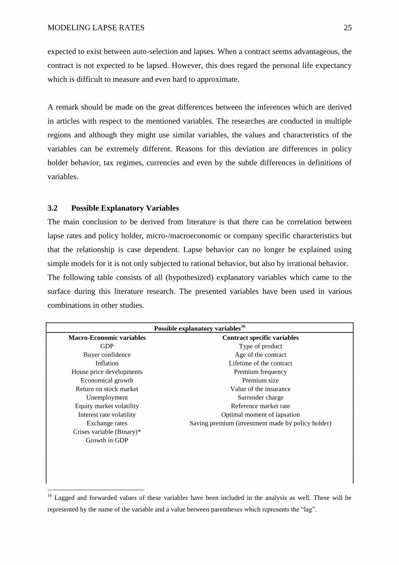
The following table consists of all (hypothesized) explanatory variables which came to the
surface during this literature research. The presented variables have been used in various
combinations in other studies.
Possible explanatory variables16
Macro-Economic variables Contract specific variables
GDP Type of product
Buyer confidence Age of the contract
Inflation Lifetime of the contract
House price developments Premium frequency
Economical growth Premium size
Return on stock market Value of the insurance
Unemployment Surrender charge
Equity market volatility Reference market rate
Interest rate volatility Optimal moment of lapsation
Exchange rates Saving premium (investment made by policy holder)
Crises variable (Binary)*
Growth in GDP
16
Lagged and forwarded values of these variables have been included in the analysis as well. These will be
represented by the name of the variable and a value between parentheses which represents the “lag”.

MODELING LAPSE RATES 26
Policy holder specific variables Company specific variables
Age of policy holder Division/part of the company
Gender Distribution channel
Widowed Negative publicity*
Marital status Crediting rate
Postal code*
New Legislation*
Mortality rate
Time variables
Ratios
Seasonal effects*
Calendar year of exposure
“*” Indicates that the variable is not mentioned in articles but is expected to be relevant.
Table 1 Possible explanatory variables
MODELING LAPSE RATES 27
Chapter 4 Predictive Models
“Generally, predictive modeling can be thought of as the application of certain algorithms and
statistical techniques to a data set to better understand the behavior of a target variable based
on the co-relationships of several explanatory variables.”17
For a predictive model to be
appropriate it needs to meet certain criteria. This section starts with an introduction to
predictive models which results in the choice for a Generalized Linear Model [GLM] as
modeling technique. Subsequently the different modeling criteria, ranging from those set by
Achmea to those set by the regulatory bodies, will be illustrated and the choice for a specific
GLM is explicated.
4.1 Predictive Models
Predictive models are favored relative to traditional models for they capture more risks and
can account for inter-variable correlation (Briere-Giroux et al., 2010). Whereas some
variables can be accurately predicted with a predictive model, others are more complex and
cannot be predicted with high accuracy. Depending on the amount of underlying drivers and
the assumed relationship between drivers and variables there are various models which can be
opted for.
The most basic type of predictive models with explanatory variables are the one-factor
models. These models suggest a significant relationship between a single variable and lapse
rates. A common predictor is the reference market rate, which is the interest rate provided by
a competitor (Briere-Giroux et al., 2010). This choice is justified by suggesting that the policy
holder (constantly) compares similar products and chooses its policy based on its relative
costs. Examples of such functions which are currently used by insurance companies are the18
:
Arctangent model:
Parabolic model: r
Exponential model:
In which
r is the monthly lapse rate
a, b, m, n are coefficients
∆ is the reference market rate minus crediting rate19
minus surrender charges
17
See Briere-Giroux et al.(2010, p.1).
18 See Kim (2005).
19 The crediting rate is the interest rate on an investment type insurance policy.
MODELING LAPSE RATES 28
CR is the crediting rate
MR is the reference market rate
Sign ( ) is +1 if ( ) is positive, -1 if ( ) is negative and 0 when ( ) is zero
Even more complex are the models which select their components and their coefficients based
on certain defined criteria and for which high mathematics/statistics is used to determine their
coefficients. In literature there are two such models which are said to be applicable in the
insurance industry. One is the classification and regression tree [CART] and the other is the
Generalized Liner Model.
CART-models produce either classification or regression trees, dependant on whether the
dependent variable is categorical or numeric. They are non-parametric forecasting methods.
The main procedure of the CART-model is the step by step division of lapse data into smaller
groups, based on binary rules. At each step the algorithm selects the variable or combination
of variables which provides the greatest purity of data in order to form homogeneous data
sets. The algorithm stops with dividing the data set as soon as an (arbitrarily) chosen criterion
has been reached. Examples of such criteria are: Equality of observations of the explanatory
variables in a given class, a minimum number of observations per node or a specific potential
of increase in data purity (Loisel & Maume-Deschamps, 2010). The advantages of this
method are that the results are easily interpretable, because of the tree structure, and that it is
nonparametric and nonlinear (StatSoft, n.d.). Another advantage is the fact that CART-models
can include continuous as well as categorical predictor variables, which is extremely useful
with variables such as gender, division and product type.
Main disadvantages are the complexity of the CART algorithms and the instability of the
model, a small change in data may lead to huge change in the outcome20
. Guszcza (2005)
states that the model does a poor job at modeling linear structure, but can be used as a pre-test
to analyze which variables or combination of variables might be explanatory. The CART-
model is just one type of tree model and by far not the most complex. Because of the
nonlinearity and its subdivision of data, the trees can provide pretty accurate results.
20
See Timofeev (2004).
MODELING LAPSE RATES 29
The second model which is mentioned in literature for the modeling lapse rates is the
generalized linear model. This model combines a number of linear variables into one
regression model and uses a link-function, a function which transforms the data distribution of
the linear variables, to predict an outcome variable, which is expected to have a distribution
from the exponential family of distributions. GLMs are favored for they can provide accurate
results when applied to lapse data, similar to the CART-models21
, while remaining
interpretable (Briere-Giroux et al., 2010).
A GLM is suited to model many different types of functions, due to its link-function, and can
predict (with) continuous as well as (with) binary variables. This characteristic is of great use
in the insurance industry since the lapse variable can be either zero or one on a policy level
and continuous between zero and one on an aggregated level. For these reasons the GLM
theory is investigated more thoroughly.
In the following two sections the requirements for lapse rate models and Achmea‟s lapse rate
model will be discussed, before going into more detail on GLMs
4.2 The Requirements of Regulatory Bodies (the DNB) for the Lapse Rate Model
With the implementation of Solvency II an amount of flexibility is given to the implementers,
enabling them to shape the regulatory capital calculation, partly, as they see fit. The main
flexibility is in the presented choice to use either a standard or an internal model. Since the
standard model is based on industry averages it might be beneficial to develop internal
model(s) whenever the company‟s risk is expected to be below industry‟s average,
considering that a decrease in modeled risk leads to a decrease in regulatory capital. The
requirements of the DNB for the model can be summarized as follows. The models should…
“…be able to provide an appropriate calculation of the SCR (Article 100);
…be an integrated part of the undertaking‟s risk management process and systems of
governance (Articles 43,110.5 and 118); and
…satisfy the tests and requirements as set out in Articles 118-123.”22
The test which is mentioned is the use test. That test will require firms “to demonstrate that
the internal model is widely used in and plays an important role in their system of governance
21
Loisel & Maume-Deschamps (2010) state that the GLM they analyzed provided more prudent results. 22
See FSA (2009a, p.15)
MODELING LAPSE RATES 30
(art 41-49), and in particular, their risk management system, decision making processes and
the ORSA (Own Risk & Solvency Assessment, ed.)” (Lloyd‟s, n.d.) The other requirements
are on statistical quality, calibration, profit & loss, validation and documentation standards.
Research presented by Deloitte (2010) states that it might be hard and too cost-/time-
consuming to develop and implement a full model -a model composed out of multiple internal
models for all risk categories. This is why the choice can be made to use the standard formula
for one or more of the Solvency II‟s risk categories. Such a combination is what is called a
partial model. Achmea chose to develop a partial model with inclusion of an internal model
for lapse rates.
4.3 Achmea’s Internal Model
The current lapse rate calculation
Currently there is no finished internal model which meets Achmea‟s as well as the DNB‟s
requirements. This means that the prescribed standard lapse rate formula is adopted, for the
time being, instead of an internal model. The calculation prescribed by the standard model for
regulatory capital held for lapse events is as described below.
The standard formula
The capital requirement for lapse risk under the standard formula is the maximum loss
resulting from one of three scenarios23
:
A permanent increase of lapse rates by 50%.
A permanent decrease of lapse rates by 50%.
A mass lapse event where 30% of the policies are surrendered at once.
Per scenario the new lapse rate is used to calculate the loss corresponding to a loss event that,
statistically speaking, occurs only once every two hundred years. The new lapse rate which is
used and to which the shocks are applied is chosen by the insurer based on its own
experience. The lapse rates which are expected, based on the insurer‟s experience, need to be,
amongst other things, plausible, testable and representative. The proposed lapse rate and the
method for obtaining it are examined by the DNB
23
See CEIOPS (2009).
MODELING LAPSE RATES 31
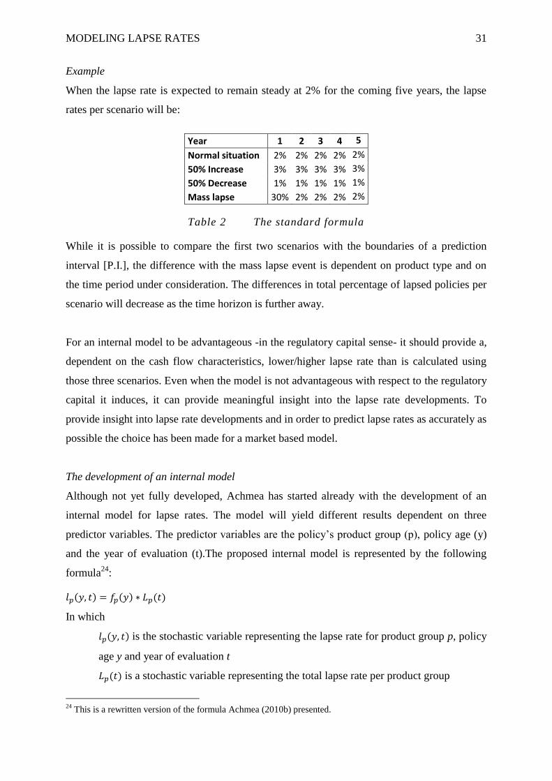
Example
When the lapse rate is expected to remain steady at 2% for the coming five years, the lapse
rates per scenario will be:
Year 1 2 3 4 5
Normal situation 2% 2% 2% 2% 2%
50% Increase 3% 3% 3% 3% 3%
50% Decrease 1% 1% 1% 1% 1%
Mass lapse 30% 2% 2% 2% 2%
Table 2 The standard formula
While it is possible to compare the first two scenarios with the boundaries of a prediction
interval [P.I.], the difference with the mass lapse event is dependent on product type and on
the time period under consideration. The differences in total percentage of lapsed policies per
scenario will decrease as the time horizon is further away.
For an internal model to be advantageous -in the regulatory capital sense- it should provide a,
dependent on the cash flow characteristics, lower/higher lapse rate than is calculated using
those three scenarios. Even when the model is not advantageous with respect to the regulatory
capital it induces, it can provide meaningful insight into the lapse rate developments. To
provide insight into lapse rate developments and in order to predict lapse rates as accurately as
possible the choice has been made for a market based model.
The development of an internal model
Although not yet fully developed, Achmea has started already with the development of an
internal model for lapse rates. The model will yield different results dependent on three
predictor variables. The predictor variables are the policy‟s product group (p), policy age (y)
and the year of evaluation (t).The proposed internal model is represented by the following
formula24
:
In which
is the stochastic variable representing the lapse rate for product group p, policy
age y and year of evaluation t
is a stochastic variable representing the total lapse rate per product group
24
This is a rewritten version of the formula Achmea (2010b) presented.

MODELING LAPSE RATES 32
is a deterministic scaling parameter for policy age y and product group p
The expected value of a stochastic variable, , is estimated by means of autoregressive
integrated moving average-models, ARIMA (0,0,0); ARIMA (0,1,0) and ARIMA (1,0,0),
which are well-known time series models, the models correspond to, respectively; a constant
with noise/trendless process, a random walk with drift and a first degree autoregressive
process (Achmea, 2010b). The ARIMA-models have some limitations of which their focus on
historical values is seen as the most disturbing for application in the life insurance industry.
The scaling parameters might make up for some of its shortcomings, although the process and
values of the scaling parameter remains unspecified. The effect of this focus on historic values
makes the model sensitive to unique events.
The added value of the research that will be done in subsequent sections, to the standard and
internal model, is the broad scope. In this research more variables are analyzed on their
significance and distribution, which is expected to lead to a more accurate result.
4.4 Generalized Linear Models
Generalized linear models represent a class of regression models, which involves more than
just linear regression models. One of the additional features is that the response variable can
have a distribution other than Normal; it can be any distribution of the exponential family of
distributions. Examples of probability distribution functions which belong to the exponential
family of distributions are: the Gaussian, Bernoulli, Binomial, Gamma, Poisson and Weibull
distribution. Another additional feature is that the relationship between the response variable
and explanatory variables can be chosen to be non-linear25
.
The composition of a GLM
A GLM consists of three components, which are (Anderson, 2010a):
1. A random component – This is the response variable (Y), it has to be identified and its
probability distribution has to be specified/assumed. In this research Y denotes the
lapse rate.
2. A systematic component – This is a set of explanatory variables (X) and
corresponding coefficients set β. A single observation is denoted as in which j
25
See Anderson (2010a) and Cerchiara et al. (2008).
MODELING LAPSE RATES 33
indicates it is the observation and m indicates it regards the variable in the
equation. The explanatory variables are entered in a linear manner, for example:
in which represents a constant.
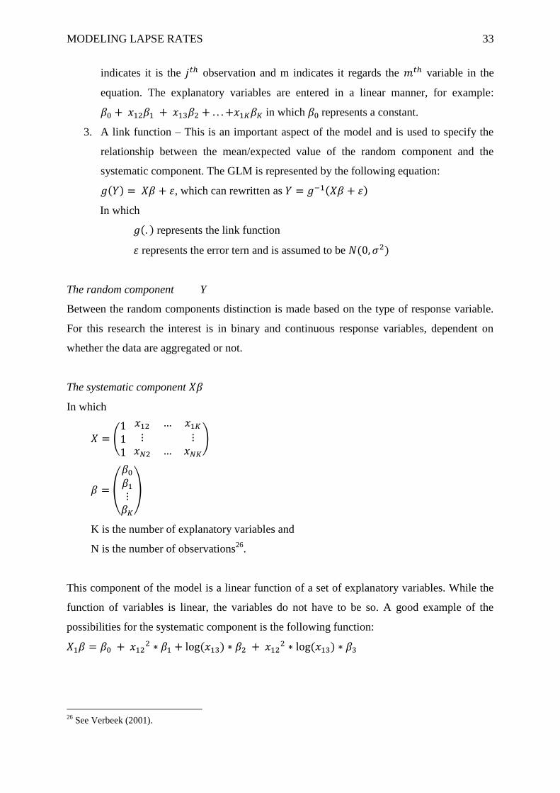
3. A link function – This is an important aspect of the model and is used to specify the
relationship between the mean/expected value of the random component and the
systematic component. The GLM is represented by the following equation:
, which can rewritten as
In which
represents the link function
represents the error tern and is assumed to be
The random component Y
Between the random components distinction is made based on the type of response variable.
For this research the interest is in binary and continuous response variables, dependent on
whether the data are aggregated or not.
The systematic component
In which
K is the number of explanatory variables and
N is the number of observations26
.
This component of the model is a linear function of a set of explanatory variables. While the
function of variables is linear, the variables do not have to be so. A good example of the
possibilities for the systematic component is the following function:
26
See Verbeek (2001).

MODELING LAPSE RATES 34
The link function
With the random component symbolizing the response variable and the systematic component
symbolizing the explanatory variables, the only thing missing (apart from the error term) is
the link between both sides; the relationship explaining how the explanatory variables relate
to the response variable. That relationship is described by the link function. The relationship
between the random component, systematic component and link-function is represented by
the following equation:
Applying a GLM involves assuming certain conditions of the data. The congruence of the
data with these assumptions should be checked before the model can be assessed.
Assumptions are made with respect to, for instance, the distribution of the variables and on
characteristics of the residuals.
Next to the assumptions that underlie GLM‟s there are certain guidelines for applying a GLM.
One guideline is to assume a linear relationship between the systematic component and the
random component when there is no reason to assume another than linear link-function to be
more appropriate. This is also the procedure which will be followed in this study. Nonetheless
the next section will be on the most relevant link-functions for binary and continuous lapse
data, to complete the theory on GLMs.
4.5 The Link Function27
Generally there are two different methods used for modeling lapse rates. The difference in
methods is in the link function and is mostly dependent on the aggregation level of the used
data. In this section the link functions for lapse data on policy as well as aggregated level are
presented.
Policy level data - Binary lapse variable
In many cases the lapse variable is recorded in such detail that its values are known per policy
and are either zero or one, representing no lapse or a lapse. This binary outcome renders a
couple of methods as inappropriate.
27
See Wei (2002).

MODELING LAPSE RATES 35
Researchers usually choose one of the following link-functions when dealing with binary
data:
Logit function,
Probit model,
In which is the inverse cumulative distribution function associated with the
standard Normal distribution.
Log-linear/Poisson
Application of one of these functions will provide an estimate which can be different from
zero or one. This is why a threshold is chosen and it is examined whether the prediction is
below or above that threshold which will determine whether the predicted value is rounded of
to zero or one.
The mentioned Poisson model assumes, amongst other things, that the changes in rate of
predictor variables have a multiplicative effect and that the variance is equal to the mean. The
Poisson model is regarded to be a suited choice for predicting extreme events. The model is
applied when the lapse rates are expected to be close to zero and when the results of the
model are used qualitative rather than quantitative (Cerchiara et al., 2008).
As shown by Anderson (2010b) there is little difference in results between the logit- and
probit-function, with the logit-function providing slightly more accurate results. Kim (2005)
also shows that the logit-function is generally better than existing surrender models which
only use a single parameter for lapse rate estimation. Congruent to those findings the logit-
function appears to be the most favored method for the modeling of lapse rates. Guszcza
(2005) compared some tree-models with logistic regression and concluded that logistic
regression outperformed the relative simple CART-model but was inferior to the more
sophisticated MARS-model. The low complexity and consequently high understandability of
logistic regression are additional reasons for the logit-function to be a suited predictor.
One of the advantages of the logit-function is that it can be used to form the odds-ratio
(Anderson, 2010b). The odds-ratio indicates how much an option is more likely than another
option. This scaling factor increases the interpretability and applicability of the model.

MODELING LAPSE RATES 36
Aggregated data - Continuous lapse variable
Not many articles on lapse rates in the insurance industry publish which link-function they
use for analyzing a continuous lapse variable.
Common link-functions are28
:
Linear regression
Logistic regression
This function is the same as the one for binary data.
Complementary log-log regression
The difference with binary data is that the predicted values are not rounded of to zero or one.
Which of the link-functions is most suited can be analyzed using either a graph, for instance a
scatterplot, or a statistical measure, for instance Pearson‟s correlation coefficient.
When the choice has been made to develop a GLM and it is hard to identify the data
distribution it is practice to start without a link function29
. This specific GLM is, as is
demonstrated above, known as the linear regression model.
Conclusion
On a policy level, where the lapse variable is either 0 or 1, the logit-link function is advised to
use with the lapse data.
On a more aggregated level, where the recorded lapse data are averages, it should be tested
which link-function suits the data the most, starting with linear regression.
28
See Fox(2008).
29 See Guyon & Elisseeff (2003).

MODELING LAPSE RATES 37
Chapter 5 Methods
This chapter starts with a quick explanation of the subjects of interest and of programs which
were used to analyze the data of those subjects. Subsequently the appliance of the linear
regression model is discussed; the procedure for forming a linear regression model is
explained, as well the assessment of certain model characteristics.
5.1 Scope of the Research
Due to several reasons lapse rates have not always been a field of study, neither in literature
nor within Achmea. This is why the data on lapses do not go as far back in time as the
company‟s origin and accurately recording of the data did not always have the highest
priority. That is also the reason why it is rather doubtful whether, in some cases, the recorded
lapse rates are just unusual or the data have not been accurately managed. Next to the state
and validity of the data, there is also the problem with obtainability of the data. Those
obstacles influenced the choice to model lapse rates just for a part of Achmea‟s portfolio. The
companies included in the analysis are CBA (Centraal Beheer Achmea) and FBTO (Friesche
Boeren en Tuinders Onderlinge). They constitute approximately 8% of Achmea‟s provisions
and are mainly oriented on the insurance market. Based on experience a difference between
individual and group contracts is suspected, which is why the lapse rates of only the
individually closed contracts are analyzed30
.
Since it cost too much time to get the needed authority to obtain the right data, only
aggregated lapse rates are available for analysis instead of policy specific data. As a result of
this unavailability of data a different modeling technique is applied than preferred, the amount
of data is restricted and consequently a lot of explanatory variables cannot be tested on
significance31
. The data available belong to the years 1996 to 2011 and were recorded on a
yearly basis. The data are not modified before analysis.
5.2 Apparatus
The policy data of Achmea‟s subsidiaries are not all recorded in a similar format. This is why
the program Data Conversion System (DCS) is used. DCS is a conversion system that can be
coded to transform the input‟s format. The conversed data are then used as input by Glean, an
analysis system. Glean is specifically designed to analyze policy data. Both programs, DCS
30
This expectation is supported by the report on persistency of the FSA (2010).
31 The little data set makes the relative influence of an observation quite high and, consequently, making the
availability of data one of the important factors which influence the results.

MODELING LAPSE RATES 38
and Glean, are developed by SunGard, a major software and technology services company
and are part of the regular data analysis process of Achmea.
After the data have been processed by Glean they are extracted and used as input for SPSS 17,
which is used for the formation of models. SPSS is a well-known statistical software program
which is developed by IBM. SPSS is promoted by IBM for its predictive analytics, the
function which is used in this research.
The graphical images which are not developed by SPSS 17 or Glean are made by programs
from the Microsoft Office 2010 package. Of this package the programs Excel and Word have
been used. It should be noted that these programs have not been included in the mathematical
part of the data-analysis.
5.3 Procedure & Measurement32
GLMs rest on certain assumptions about the data, assumptions which justify the use of the
regression models for purpose of prediction. There are four principal assumptions which are
linearity of the relationship between the dependent and independent variables and
independence, homoscedasticity33
and normality of the errors. Apart from those principal
assumptions there are conditions which should be tested to justify the application of statistical
measures and goodness-of-fit of the model. The procedure of the data-analysis can be
described by the following steps:
Conditions which can be checked before formation of a model
1. No outlier distortion
2. A linear relationship between dependent and independent variables
3. Independence of observations
Condition which can be checked after formation of a model
4. No multicollinearity34
5. Representativeness of the sample and proper specification of the model (no variables
were omitted)
32
The following procedure is applicable to continuous lapse data. The procedure described might differ from
those actions which should be taken when analyzing binary data. 33
Homoscedasticity states that all error terms have the same variance.
34 No multilcollinearity refers to the assumption that none of the explanatory variables is an exact linear
combination of the other explanatory variables, which would render the variable redundant.
MODELING LAPSE RATES 39
Selection of a model (in case of multiple possible models)
Conditions which can be checked after selection of the model
6. Normality of the residuals
7. Equality in variance of the errors (homogeneity of residual variance)
8. No auto-correlation of the errors
In the following subsections the procedure of verifying whether the assumptions/requirements
are fulfilled is described as well as the procedure for assessing the model.
5.3.1 Conditions which can be checked before formation of a model.
Assumption 1 No outlier distortion
Outliers are observations which are classified as being abnormal. Outliers are said to
influence the model in a negative way, since a model is fitted to the observation‟s data using
the leased squares formula. The least squares formula can be used when there are more
equations than unknowns; it provides the overall solution which minimizes the sum of the
squares of the errors made in solving every single equation.
When data are expected to be erroneous they can be ignored, excluded from the analysis,
transformed or the variable can be modified/excluded. The benchmark for outliers is chosen
rather arbitrarily. Usually observations are classified as outliers based on their deviation from
the mean, expressed in standard deviations of the sample. Outliers can be detected using a
boxplot. A boxplot calculates a measure called interquartile range (IQR), which is the
difference between the third and first quartile Subsequently an outlier is classified, in this
case, as all values which are 1.5* IQR below the first or above the third quartile.
However, when an outlier did not arise due to an error or an event that is known to occur once
and once only, the exclusion of the data might have negative consequences. The exclusion of
the data will make the model sensitive to the particular event. For this reason exclusion of
outliers is not done in this research unless it can be underpinned by a better reason than the
1.5*IQR measure.
Assumption 2 A linear relationship between dependent and independent variables
One of the main assumptions is the existence of a linear relationship between the dependent
and independent variables. This linearity can be assessed in two manners, namely;
MODELING LAPSE RATES 40
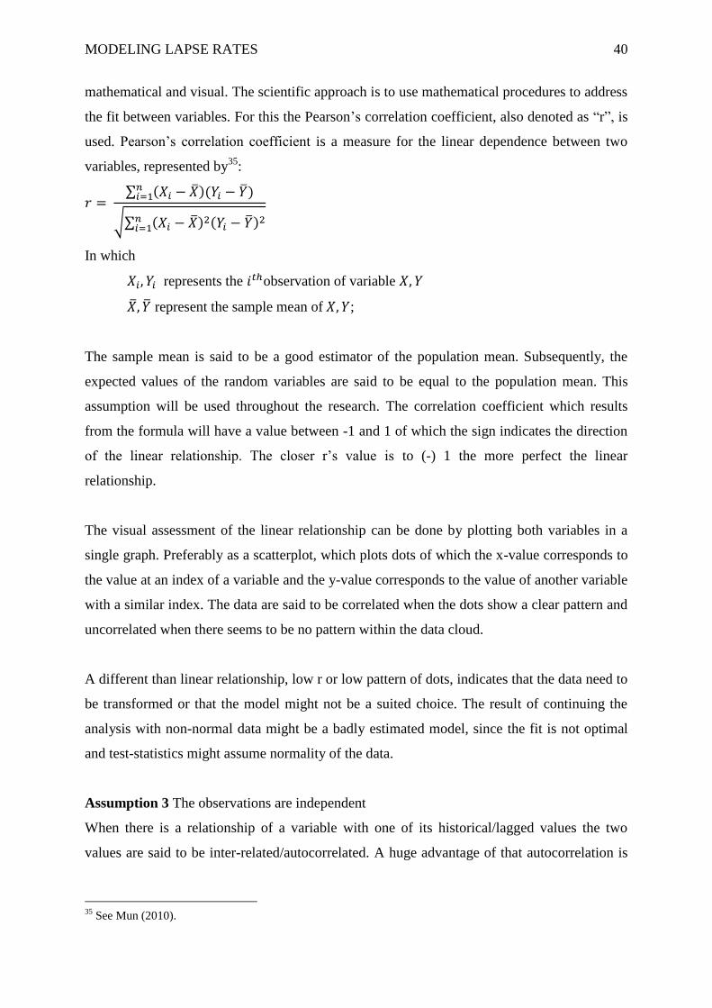
mathematical and visual. The scientific approach is to use mathematical procedures to address
the fit between variables. For this the Pearson‟s correlation coefficient, also denoted as “r”, is
used. Pearson‟s correlation coefficient is a measure for the linear dependence between two
variables, represented by35
:
In which
represents the observation of variable
represent the sample mean of ;
The sample mean is said to be a good estimator of the population mean. Subsequently, the
expected values of the random variables are said to be equal to the population mean. This
assumption will be used throughout the research. The correlation coefficient which results
from the formula will have a value between -1 and 1 of which the sign indicates the direction
of the linear relationship. The closer r‟s value is to (-) 1 the more perfect the linear
relationship.
The visual assessment of the linear relationship can be done by plotting both variables in a
single graph. Preferably as a scatterplot, which plots dots of which the x-value corresponds to
the value at an index of a variable and the y-value corresponds to the value of another variable
with a similar index. The data are said to be correlated when the dots show a clear pattern and
uncorrelated when there seems to be no pattern within the data cloud.
A different than linear relationship, low r or low pattern of dots, indicates that the data need to
be transformed or that the model might not be a suited choice. The result of continuing the
analysis with non-normal data might be a badly estimated model, since the fit is not optimal
and test-statistics might assume normality of the data.
Assumption 3 The observations are independent
When there is a relationship of a variable with one of its historical/lagged values the two
values are said to be inter-related/autocorrelated. A huge advantage of that autocorrelation is
35
See Mun (2010).
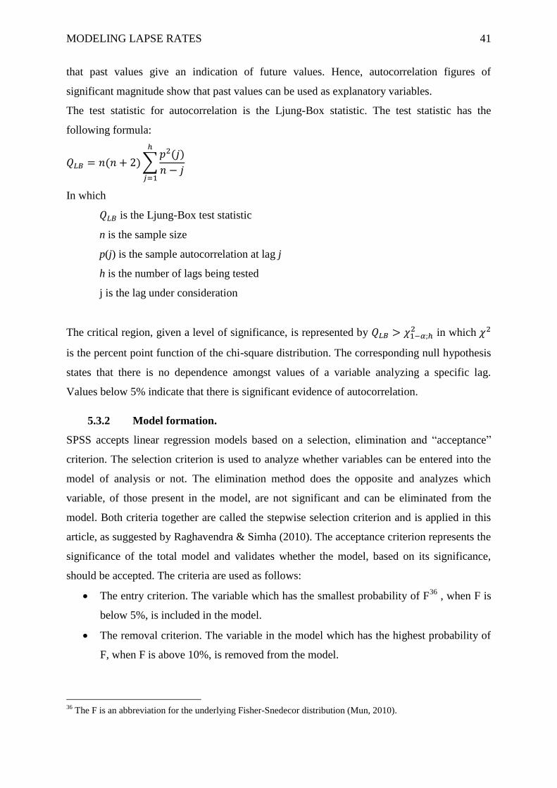
MODELING LAPSE RATES 41
that past values give an indication of future values. Hence, autocorrelation figures of
significant magnitude show that past values can be used as explanatory variables.
The test statistic for autocorrelation is the Ljung-Box statistic. The test statistic has the
following formula:
In which
is the Ljung-Box test statistic
n is the sample size
p(j) is the sample autocorrelation at lag j
h is the number of lags being tested
j is the lag under consideration
The critical region, given a level of significance, is represented by in which
is the percent point function of the chi-square distribution. The corresponding null hypothesis
states that there is no dependence amongst values of a variable analyzing a specific lag.
Values below 5% indicate that there is significant evidence of autocorrelation.
5.3.2 Model formation.
SPSS accepts linear regression models based on a selection, elimination and “acceptance”
criterion. The selection criterion is used to analyze whether variables can be entered into the
model of analysis or not. The elimination method does the opposite and analyzes which
variable, of those present in the model, are not significant and can be eliminated from the
model. Both criteria together are called the stepwise selection criterion and is applied in this
article, as suggested by Raghavendra & Simha (2010). The acceptance criterion represents the
significance of the total model and validates whether the model, based on its significance,
should be accepted. The criteria are used as follows:
The entry criterion. The variable which has the smallest probability of F36
, when F is
below 5%, is included in the model.
The removal criterion. The variable in the model which has the highest probability of
F, when F is above 10%, is removed from the model.
36
The F is an abbreviation for the underlying Fisher-Snedecor distribution (Mun, 2010).
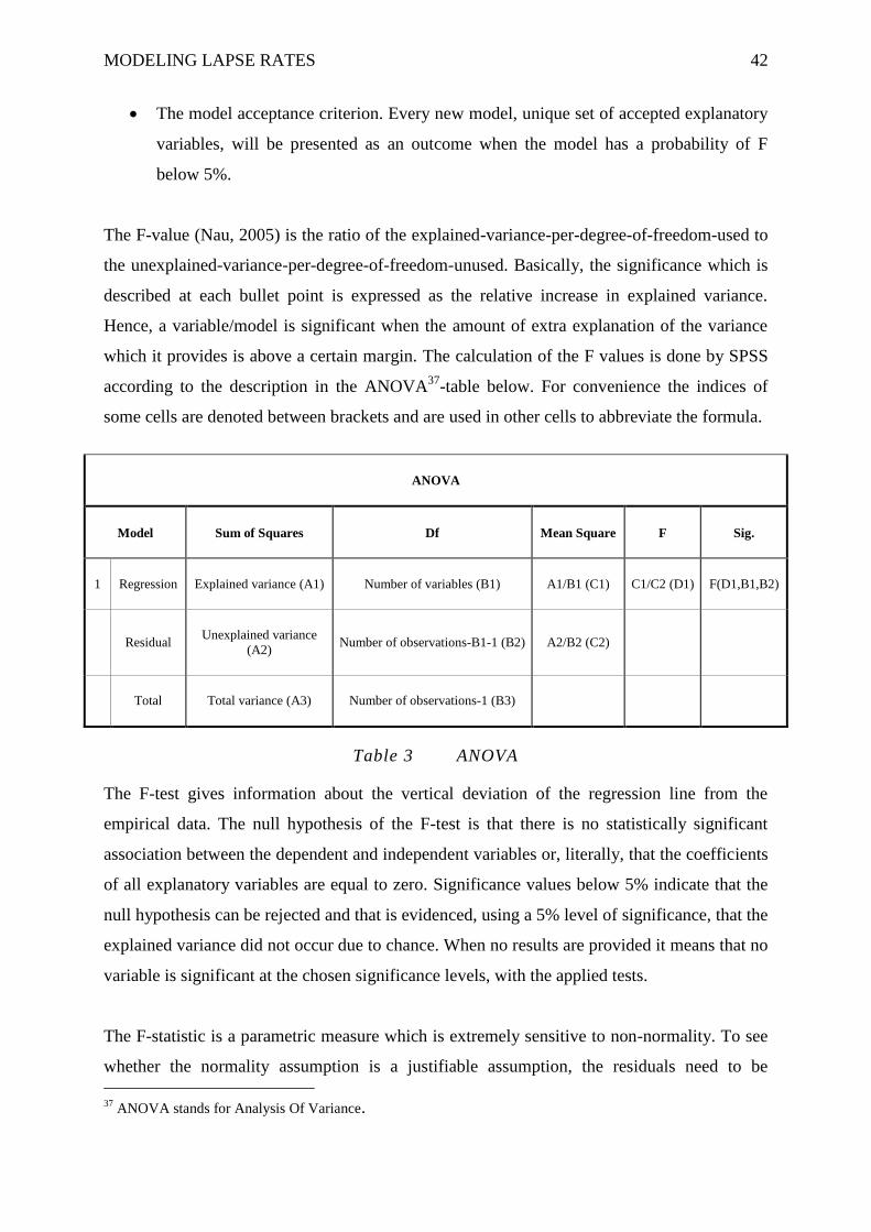
MODELING LAPSE RATES 42
The model acceptance criterion. Every new model, unique set of accepted explanatory
variables, will be presented as an outcome when the model has a probability of F
below 5%.
The F-value (Nau, 2005) is the ratio of the explained-variance-per-degree-of-freedom-used to
the unexplained-variance-per-degree-of-freedom-unused. Basically, the significance which is
described at each bullet point is expressed as the relative increase in explained variance.
Hence, a variable/model is significant when the amount of extra explanation of the variance
which it provides is above a certain margin. The calculation of the F values is done by SPSS
according to the description in the ANOVA37
-table below. For convenience the indices of
some cells are denoted between brackets and are used in other cells to abbreviate the formula.
ANOVA
Model Sum of Squares Df Mean Square F Sig.
1 Regression Explained variance (A1) Number of variables (B1) A1/B1 (C1) C1/C2 (D1) F(D1,B1,B2)
Residual Unexplained variance
(A2) Number of observations-B1-1 (B2) A2/B2 (C2)
Total Total variance (A3) Number of observations-1 (B3)
Table 3 ANOVA
The F-test gives information about the vertical deviation of the regression line from the
empirical data. The null hypothesis of the F-test is that there is no statistically significant
association between the dependent and independent variables or, literally, that the coefficients
of all explanatory variables are equal to zero. Significance values below 5% indicate that the
null hypothesis can be rejected and that is evidenced, using a 5% level of significance, that the
explained variance did not occur due to chance. When no results are provided it means that no
variable is significant at the chosen significance levels, with the applied tests.
The F-statistic is a parametric measure which is extremely sensitive to non-normality. To see
whether the normality assumption is a justifiable assumption, the residuals need to be
37
ANOVA stands for Analysis Of Variance.
MODELING LAPSE RATES 43
analyzed and checked on normality. If the data pass the normality test the F-statistic can be
used. Otherwise, with all things remaining equal, another test statistic should be chosen. An
alternative which is more robust is Levene‟s test (National Institute of Standards and
Technology & Sematech, n.d.). This test can be thought of when the normality assumption is
questioned. The model can be accepted when the significance is sufficient and the
assumptions and results are acceptable.
Next to the mathematical test there is again a visual test. The historical values of the
explanatory variables can be used to predict the lapse rates and a comparison can be made by
plotting real and predicted values for the year 2011 in combination with a 99.5% prediction
interval. The upper and lower bound of the 99.5% P.I. can be compared with the 50% in- and
decrease of the standard formula. Whether the results of the model are more advantageous for
the calculation of capital requirements et cetera will be dependent on the effects of lapses on
the profitability of product groups.
Before any inferences can be made there are a few other assumptions which should be
checked, the corresponding tests are described below.
5.3.3 Condition which can be checked after formation of a model.
Assumption 4 No multicollinearity
When the term multicollinearity is used in the context of multiple regression it concerns the
event of strong correlation amongst de predictor variables (Doorn, 2006). When there are
variables included in a model which experience high multicollinearity their individual effect
on the dependent variable becomes an arbitrary value. This might make the exclusion of one
of the mutual dependent variables inevitable. Another issue with multicollinearity is that some
independent variables are redundant with one and another. As a consequence one or more of
the variables do not add any predictive value, while they do cost a degree of freedom. This
will consequently weaken the analysis. Logically this type of multicollinearity can only occur
when more than one variable is present in the model. When the model consists of only one
variable the term multicollinearity has a totally different meaning. In that case the term
multicollinearity refers to the problem of having multiple different values of the response
variable related to one value of the independent variable. This type of multicollinearity would
provide difficulties in assessing the best regression coefficient for the regression line.
MODELING LAPSE RATES 44
The multicollinearity will be assessed based on the “variance inflation factor” (VIF). The VIF
can be calculated by (Yaffee, 2004):
In which is the coefficient of determination of the regression equation.
While there are no clear boundaries for the VIF-values, it is known that low values- with a
minimum of 1- indicate low multicollinearity. As a rule of thumb Yaffee (2004) suggests to
use a VIF-value of 10 as a boundary, with which values above 10 indicate alarming
multicollinearity. Next to the VIF-value SPSS also provides other measures for
intercorrelation among independent variables like tolerance and the variance proportion. Both
measures are related to the variance inflation factor.
Assumption 5 The sample is representative and the model has been properly specified (no
variables were omitted)
The representativeness of the sample is usually based on the randomness in the selection of
the sample. The sample used, FBTO and CBA data from 1996 to 2011, encompasses many
product groups and many policies. However, it is not known whether the lapse rate levels or
developments are representative for Achmea as a holding. This is why the research will only
help to make inferences on the lapse rates of this particular sample while leaving the
generalizability to be a question mark. Eventually, after accepting a model, the congruence of
the predicted lapse rates with the real lapse rates can be assessed. The deviation between both
rates will be an indication of the accuracy with which the rates can be predicted. The
deviation will indicate whether the model is a fine predictor, variables are missing or that the
deviation in prediction comes down to an unpredictable error term. In advance it can be noted
that the lack of many policy (holder) related data/variables might ensure that some relevant
variables are omitted, since those variables would probably help explaining individual
behavior more extensively.
5.3.4 Selection of a model.
Whenever more than one model is accepted using the prescribed test statistics the different
models should be compared. Next to the already explained statistics there is another measure,
the adjusted r square, which penalizes the model for the inclusion of extra variables. This
effect is created by adding the degrees of freedom to the calculation of the by the model
MODELING LAPSE RATES 45
accounted for proportion of the variation in the dependent variable (SAP, n.d.). In other
words, the additional explanatory power which is created by adding a variable to the model is
estimated. As a consequence the value of the measure decreases when the addition of an
explanatory variable does not increase the residual sum of squares more than would be
expected by chance. So, the model with the highest adjusted r square model is chosen to
represent the model with the highest goodness-of-fit.
5.3.5 Conditions which can be checked after selection of the model.
Assumption 6 The residuals are normally distributed
For this assessment the Kolmogorov-Smirnov (K-S) test is used. More specifically it is the
one-sample K-S test which is used. This test compares a sample with a reference probability
distribution, in this case with the Normal distribution. The hypotheses of this test are (Gate,
2000):
: There is no difference between the distribution of the data set and a normal one 38
: There is a difference between the distribution of the data set and normal 39
In the case of normal distributed residuals the outcome of the K-S test will have to be a level
of significance above 5%. A significance above 5% leads to the inference that should be
accepted, so the hypothesis that the residuals are normally distributed is accepted. As a visual
verification of the outcome of the K-S test the residuals can be shown by a histogram. For
convenience the normal-curve can be superimposed as a line, so that the normality of the data
can be observed by looking at its deviation from the superimposed curve.
Assumption 7 The errors have equal variances (homogeneity of residual variance)
Assessment of the equality of the variance of the errors is conducted by plotting the
standardized residuals versus the standardized predicted values. Homogeneity of residual
variance requires that the residuals per observation remain approximately constant as the
predicted value changes. An approximately constant level of variances would indicate that the
variance of the residuals is independent of the predicted value. Heteroscedasticity might occur
when some variables are skewed while others are not. This means that when the data has
passed the test for normality the chance of the data being homoscedastic will increase.
38
is the abbreviation of the null hypothesis.
39 is the abbreviation of the alternative hypothesis.
MODELING LAPSE RATES 46
Although violation of the assumption of homoscedasticity will not invalidate the regression
model, it will weaken it.
Assumption 8 The errors are not autocorrelated
This assumption is checked in a similar manner as assumption 3.
The independence of the residuals is tested mathematically and visually verified. The
mathematical interpretation of the level of dependence amongst the residuals is done using the
Ljung-Box statistic. The null-hypothesis of this test is that the data are random/not related to
their historical values, while rejecting this hypothesis would mean that the data are dependent
on historical values.
The independence of the residuals can be verified by plotting the residuals over time.
Dependence is demonstrated by the display of a pattern in the residuals over time.
Other model statistics
Closely related to r is the r square(d) statistic. R squared ( ) is the proportion of variation in
the dependent variable which is explained by the model. As r squared is literally the square of
r, it can be calculated by multiplying r by itself. The result will be a positive figure between 0
and one. A -value of one indicates a perfect explanation of the variance of the dependent
variable by the model.
5.3.6 Product groups for which models are formed.
For every product group, of which data is available, a different model will be formed, since
their underlying parameters are assumed to deviate significantly.
The product groups are provided by Achmea and the list is composed out of the following
groups:
Mortgages. A mortgage is a security interest in real property held by a lender as a
security for a debt, usually a loan of money. A mortgage will give profits from
investment fees and related risk products.
Lapses of a mortgage are expected to be sensitive to macroeconomic changes, such as
market interest.
Risk. The product group Risk contains term life insurance products (term assurance),
that is a life insurance which provides coverage at a fixed rate of payments for a

MODELING LAPSE RATES 47
limited period of time, the relevant term. After this term the policy expires and the
assured life is not covered anymore. It is the least expensive insurance type because
savings are not financed.
Term insurance is therefore expected not to be very sensitive to market interest, but is
probably sensitive to the liquidity position of the assured.
Savings (regular premium). Non-linked (traditional) insurance savings products
financed by regular premiums [RP] are comparable to bank savings. The difference
with bank savings is that insurance products must have an element of risk for the
insurance company or the insured.
Therefore a term insurance is attached to the savings policy, negative or positive risk
can both be attached. Savings policies can have a clause (tax related) that will prevent
lapses.
Savings (single premium). Non-linked (traditional) insurance savings products
financed by single premiums [SP] are comparable to the savings products with regular
premium payments. Since there is no obligation for the policyholder to pay future
premiums the emergency fund hypothesis seems most appropriate.
Unit-Linked (regular premium). Unit-linked insurance savings products financed by
regular premiums are comparable to Savings. The fund development of a unit-linked
product is very volatile due to the market returns (stock and interest returns).
Consequently lapses are expected to be negatively correlated with stock market
developments.
Unit-Linked (single premium). Unit-linked insurance savings products financed by
single premiums are comparable to Savings.
Whole life & Funeral. The whole life insurance (permanent insurance) and funeral
products have the same coverage as the risk products (term insurance) with a main
difference in the coverage term. Whole life and funeral products have a permanent
coverage until the insured deceases. Therefore the products must include a savings
part because the sum assured will be paid in the end. The savings part (technical
reserve) will in most policy agreements not be paid to the insured when the policy is
lapsed. Lapses are expected to have the same pattern as term insurance products.
MODELING LAPSE RATES 48
5.3.7 Additional research.
Two analyses have been chosen as additional research topics, namely:
1. The assumption of dissimilarity of the lapse rate development per product group is
tested, to verify that a different model per product group is essential.
2. For the group “whole life & funeral” the data of 1 and 5 year old insurances will be
analyzed, apart from the aggregated “whole life & funeral” data. This test is performed
to evidence the hypothesis that the age, or duration, of an insurance has influence on
the corresponding lapse behavior
5.4 (Possible) Limitations
Since the data set is small and the list of possible explanatory variables is only
composed of macro-economic variables there is a possibility that no model will pass
the significance tests.
The lack of policy data on policyholder characteristics might limit the insight the
model will provide in individual behavior, which might have consequence for the
goodness-of-fit of the model.
The data set does not include many observations. This absence of a long history will
limit the generalization of the model and might make it hard to obtain a model with a
high statistical significance.
Some of the measures which test the satisfaction of underlying assumptions might
disapprove the model(ing) choice. It will depend on the measure whether the incorrect
assumptions will jeopardize the results.
It is not analyzed whether the lapse data of CBA and FBTO deviate from Achmea‟s
aggregated lapse data; therefore it is not known whether this data set is representative
for the holding.
Due to a maximum availability of two future values of the explanatory variables the
lapse rate estimations can only be done for the near future.
Note: The standard model predicts lapse rates and assumes subsequent lapse rates to
be equal to the one-year future rate. The assumption of constant future lapse rates can
be applied to the models which will be developed as well.
MODELING LAPSE RATES 49
Chapter 6 Data and Analysis
This chapter is divided into two parts. Part one is on the used data set and explains which data
sources have been chosen. Part two consists of a description of the actual data-analysis for
one product group, which is followed by the corresponding results of the other product groups
and ends with the results of the two additional researches.
6.1 Data Set
The specific range of available lapse data is the data from 1996, on a yearly basis, until 2011.
The rate corresponding to the year 2011 is omitted from the analysis. These data have been
omitted since the year is not yet finished and it is not assumed that the number of lapse events
which have occurred during the first months is representative for the number of lapses during
the last months of 2011. As indicated before it is not analyzed whether the lapse data of CBA
and FBTO deviate from Achmea‟s aggregated lapse data.
The data on Gross Domestic Product [GDP] are provided by the European Central Bank
[ECB] (2011) which collects its data in cooperation with the DNB. As data on the reference
rate the 5-years treasury rate has been used. This rate is quoted by the Federal Reserve System
[FED] (n.d.). The choice has been made for data of the FED instead of the ECB, this has been
done since ECB recordings of Dutch treasury rates do not go back further than 1999.
As a stock market for comparison the Amsterdam Exchange Index [AEX] has been chosen,
which represents a maximum of 25 of the most actively traded securities that trade on
Euronext Amsterdam. The data on this variable are provided by Yahoo (n.d.). It should be
noted that there is some criticism on the relevance of a national index due to the
internationalization of investors their operations. Other criticism is on the AEX for not
representing the whole Dutch market and for including multinationals which lack significant
bonding with the Netherlands.
The data on growth in GDP, buyer confidence, inflation and unemployment are extracted
from the database of the Centraal Planbureau [CPB] (2011). It is mentioned in articles, and
apparent from the data, that the data of the CPB differ greatly from those of the World Bank„s
database. This deviation is, however, no longer present in the years which are of interest for
this research.
MODELING LAPSE RATES 50
Finally there were two macro events chosen which represented moments of extreme
circumstances. The first year in which an extreme situation happened was 1999, in which a
huge increase in lapse rates occurred, probably, due to the immense upcoming popularity of
unit linked mortgages (Achmea, 2010b). The second was the stock market crash during the
subprime mortgages crisis which is expected to have had its impact in 2008. The dot-com
bubble which took place in 2000 does not show any visual influence on the lapse rates. Since
it is hard to predict the occurrence of an extreme event, let alone the impact of the specific
event, it is unadvisable to include such dummy variables in the model. Because of the
uncertainty surrounding the variable it will only make sense when the events are expected to
have similar impact and future extreme events have similar influence and are predictable.
6.2 Analysis
The analysis of lapse data has been conducted a total of 9 times. Seven models have been
formed for the different product groups and two for the additional studies. That is why the
procedure, which is explained in the previous section, will be described only once using the
whole life & funeral data. This section will end with a summary of the important statistics and
conclusions regarding the other 8 models. It is important to note that all macro-economic
variables have been standardized, using their first value, since the values of some variables
were of immense magnitude.

MODELING LAPSE RATES 51
6.2.1 Formation of the model.
In this subsection the steps described in chapter 5 will be elaborated with use of the actual
data.
Assumption 1 No outlier distortion
Figure 1 displays the boxplot based on the whole life & funeral data.
Figure 1 Boxplot of the whole life & funeral lapse data
Based on the box plot the events 4 and 5 are classified as outliers, these points correspond to
the lapse rates of 1999 and 2000. SPSS uses two kinds of indicators for outliers, dots and
stars. Of these indicators stars are “extreme” outliers, those which are more than 3*IQR below
the first or above the third quartile, and the dots represent “normal” outliers, those which are
more than 1.5*IQR, but less than 3*IQR below the first or above the third quartile. When
further research indicates that the data appear too skewed to be normal these events can be
investigated on their influence on the data set. For now there is no reason to exclude the
observations.
Note that exclusion of the years 1999 and 2000 will decrease the small data set even further.
A boxplot without the two observations indicates that the skewness is diminished and also
shows that there are still outliers detectable in the remaining data set.

MODELING LAPSE RATES 52
Assumption 2 A linear relation between the dependent and independent variables
The two manners in which the dependency is analyzed is by using the r-measure and a
scatterplot. The following table lists the scatterplots of the lapse rates for Whole life and
Funeral insurances and each of the predictor variables. The figures are arranged on a
descending order based on their r (squared) statistic. Each figure is composed out of lapse
rate, represented on the y-axis, and a specific variable, represented on the x-axis. The specific
variable is one of macro-economic variables from the list of possible explanatory variables
and is each time denoted above the scatterplot.
Expl.
Variable GDP (+1) Buyer Confidence (-1) Lapse rate (-1)
R-statistic -0.916 0.895 0.772
R-squared 0.839 0.801 0.595
Scatterplot
Expl.
Variable
Return on Stock Market
(-2) Reference Market Rate
Return on Stock Market
(-1)
R-statistic 0.750 0.666 0.615
R-squared 0.562 0.444 0.378
Scatterplot
Expl.
Variable
First difference in lapse
rates Unemployment (+1) Growth in GDP
R-statistic 0.551 -0.440 0.426
R-squared 0.303 0.194 0.182
Scatterplot
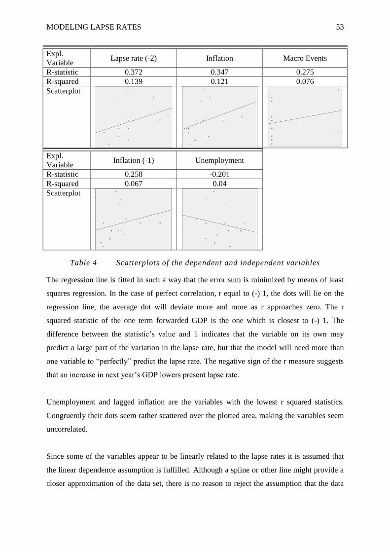
MODELING LAPSE RATES 53
Expl.
Variable Lapse rate (-2) Inflation Macro Events
R-statistic 0.372 0.347 0.275
R-squared 0.139 0.121 0.076
Scatterplot
Expl.
Variable Inflation (-1) Unemployment
R-statistic 0.258 -0.201
R-squared 0.067 0.04
Scatterplot
Table 4 Scatterplots of the dependent and independent variables
The regression line is fitted in such a way that the error sum is minimized by means of least
squares regression. In the case of perfect correlation, r equal to (-) 1, the dots will lie on the
regression line, the average dot will deviate more and more as r approaches zero. The r
squared statistic of the one term forwarded GDP is the one which is closest to (-) 1. The
difference between the statistic‟s value and 1 indicates that the variable on its own may
predict a large part of the variation in the lapse rate, but that the model will need more than
one variable to “perfectly” predict the lapse rate. The negative sign of the r measure suggests
that an increase in next year‟s GDP lowers present lapse rate.
Unemployment and lagged inflation are the variables with the lowest r squared statistics.
Congruently their dots seem rather scattered over the plotted area, making the variables seem
uncorrelated.
Since some of the variables appear to be linearly related to the lapse rates it is assumed that
the linear dependence assumption is fulfilled. Although a spline or other line might provide a
closer approximation of the data set, there is no reason to reject the assumption that the data

MODELING LAPSE RATES 54
experience linear dependency. A double-check of the linear relationship assumption will
occur in the next step, the model formation.
Assumption 3 The observations are independent
The test for autocorrelation amongst observations is performed using the Ljung-Box test. The
significance values which correspond to the Ljung-Box statistic are presented in the last
column of the table which is presented below.
Autocorrelations
Series:lapse rate
Lag Autocorrelation Std. Errora Ljung-Box Statistic
Value Df Sig.b
1 0,683 0,234 8,492 1 0,004
2 0,335 0,226 10,690 2 0,005
3 0,117 0,217 10,983 3 0,012
4 -0,042 0,208 11,023 4 0,026
5 -0,070 0,198 11,147 5 0,049
6 -0,072 0,188 11,294 6 0,080
7 -0,223 0,177 12,884 7 0,075
8 -0,316 0,166 16,527 8 0,035
9 -0,358 0,153 21,967 9 0,009
10 -0,329 0,140 27,485 10 0,002
11 -0,221 0,125 30,596 11 0,001
12 -0,094 0,108 31,345 12 0,002
13 0,023 0,089 31,412 13 0,003
a. The underlying process assumed is independence (white noise).
b. Based on the asymptotic chi-square approximation
Table 5 Autocorrelation of the lapse rates
The figures indicate that all lagged values, apart from lag 6 and 7, experience autocorrelation
which is significant at a 5% level of significance. Based on the significant autocorrelation
mall lagged values, apart from those of lag 6 and 7 can be included in the data analysis. A
consequence is that every included lagged value will decrease the amount of observations,
which is already little. For this reason the choice has been made to include the first and
second lag only40
.
40
Subsequent tests indicated that the autocorrelation at 3,4 and 5 lags did not appear to be significant enough to
be included in the model.

MODELING LAPSE RATES 55
Model formation
Based on the entry, removal and acceptance criterion SPSS provided the following models:
Model 1: ; and
Model 2:
Model 3:
The F-value and probability of F are presented in the following table.
Model Sum of Squares df Mean Square F Sig.
1
Regression 0,00018 1 0,000184 57 (11* )a
Residual 0,00004 11 0,000003
Total 0,00022 12
2
Regression 0,00020 2 0,000100 50 (6* )b
Residual 0,00002 10 0,000002
Total 0,00022 12
3
Regression 0,00021 3 0,000070 61 (3* )c
Residual 0,00001 9 0,000001
Total 0, 00022 12
a. Predictors: (Constant), GDP (+1)
b. Predictors: (Constant), GDP (+1), Buyer Confidence (-1)
c. Predictors: (Constant), GDP (+1), Buyer Confidence (-1), Unemployment
d. Dependent Variable: Lapse rate
Table 6 ANOVA of model 1, 2 and 3
As previously mentioned the null hypothesis of the F-test is that there is no statistically
significant association between the dependent and independent variables. All three models
have level of significance far below 5%, meaning that the null hypothesis, that all of the
coefficients of the explanatory variables are equal to zero, is rejected. Hence, it can be
concluded that, using a 5% level of significance, at least one of the coefficients is not equal to
zero.
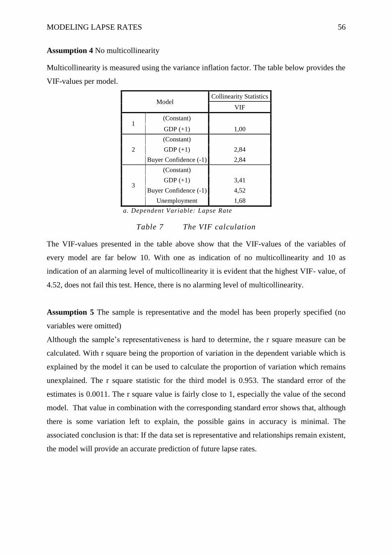
MODELING LAPSE RATES 56
Assumption 4 No multicollinearity
Multicollinearity is measured using the variance inflation factor. The table below provides the
VIF-values per model.
Model Collinearity Statistics
VIF
1 (Constant)
GDP (+1) 1,00
2
(Constant)
GDP (+1) 2,84
Buyer Confidence (-1) 2,84
3
(Constant)
GDP (+1) 3,41
Buyer Confidence (-1) 4,52
Unemployment 1,68
a. Dependent Variable: Lapse Rate
Table 7 The VIF calculation
The VIF-values presented in the table above show that the VIF-values of the variables of
every model are far below 10. With one as indication of no multicollinearity and 10 as
indication of an alarming level of multicollinearity it is evident that the highest VIF- value, of
4.52, does not fail this test. Hence, there is no alarming level of multicollinearity.
Assumption 5 The sample is representative and the model has been properly specified (no
variables were omitted)
Although the sample‟s representativeness is hard to determine, the r square measure can be
calculated. With r square being the proportion of variation in the dependent variable which is
explained by the model it can be used to calculate the proportion of variation which remains
unexplained. The r square statistic for the third model is 0.953. The standard error of the
estimates is 0.0011. The r square value is fairly close to 1, especially the value of the second
model. That value in combination with the corresponding standard error shows that, although
there is some variation left to explain, the possible gains in accuracy is minimal. The
associated conclusion is that: If the data set is representative and relationships remain existent,
the model will provide an accurate prediction of future lapse rates.

MODELING LAPSE RATES 57
Selection of a model
Three models are accepted based on the first criteria and not one of them experiences
significant multicollinearity. In the figure below some comparable statistics of the models are
presented.
Model R R Square Adjusted R Square Std. Error of the Estimate
1 0,916a 0,839 0,824 0,0018
2 0,954b 0,910 0,892 0,0014
3 0,976c 0,953 0,938 0,0011
a. Predictors: (Constant), GDP(+1)
b. Predictors: (Constant), GDP(+1), Buyer Confidence (-1)
c. Predictors: (Constant), GDP(+1), Buyer Confidence (-1), Unemployment
d. Dependent Variable: Lapse rate
Table 8 Model summary
Based on all of the values in the model summary it can be concluded that the third model
outperforms the first two regarding explanatory power. The adjusted r square measure is
higher and, logically, the standard error of the estimate is lower. The standard deviation of
the lapse variable is 0.0043. The reduction in the standard error of approximately 75%, from
0.0043 to 0.0011, indicates that the model has a better goodness-of-fit than the mean of the
sample does (Kiesenbauer, 2011). Figure 5 displays the actual lapse rates in combination with
the third model. The figure strengthens the conclusion that the model is preferred above using
the mean of the sample as prediction.
The tests which follow are all performed using model 3.
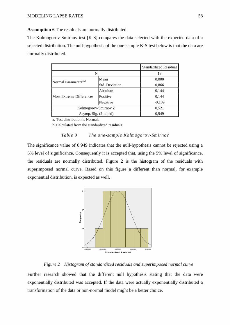
MODELING LAPSE RATES 58
Assumption 6 The residuals are normally distributed
The Kolmogorov-Smirnov test [K-S] compares the data selected with the expected data of a
selected distribution. The null-hypothesis of the one-sample K-S test below is that the data are
normally distributed.
Standardized Residual
N 13
Normal Parametersa,,b
Mean 0,000
Std. Deviation 0,866
Most Extreme Differences
Absolute 0,144
Positive 0,144
Negative -0,109
Kolmogorov-Smirnov Z 0,521
Asymp. Sig. (2-tailed) 0,949
a. Test distribution is Normal.
b. Calculated from the standardized residuals.
Table 9 The one-sample Kolmogorov-Smirnov
The significance value of 0.949 indicates that the null-hypothesis cannot be rejected using a
5% level of significance. Consequently it is accepted that, using the 5% level of significance,
the residuals are normally distributed. Figure 2 is the histogram of the residuals with
superimposed normal curve. Based on this figure a different than normal, for example
exponential distribution, is expected as well.
Figure 2 Histogram of standardized residuals and superimposed normal curve
Further research showed that the different null hypothesis stating that the data were
exponentially distributed was accepted. If the data were actually exponentially distributed a
transformation of the data or non-normal model might be a better choice.
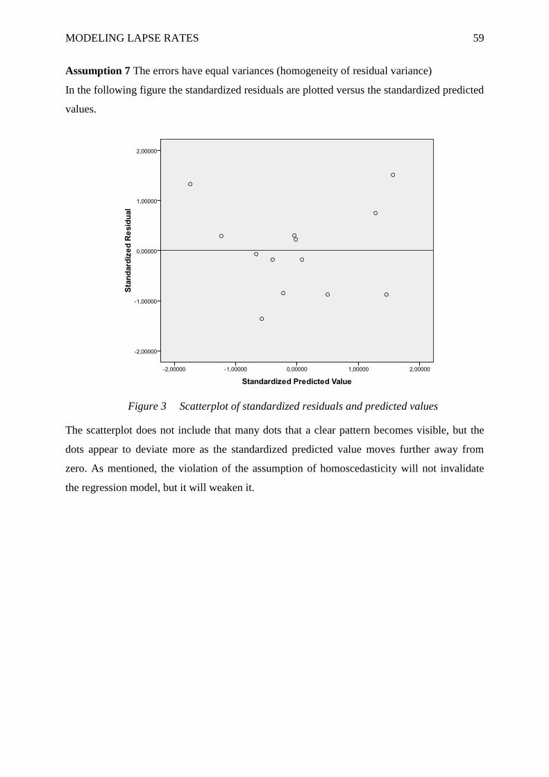
MODELING LAPSE RATES 59
Assumption 7 The errors have equal variances (homogeneity of residual variance)
In the following figure the standardized residuals are plotted versus the standardized predicted
values.
Figure 3 Scatterplot of standardized residuals and predicted values
The scatterplot does not include that many dots that a clear pattern becomes visible, but the
dots appear to deviate more as the standardized predicted value moves further away from
zero. As mentioned, the violation of the assumption of homoscedasticity will not invalidate
the regression model, but it will weaken it.
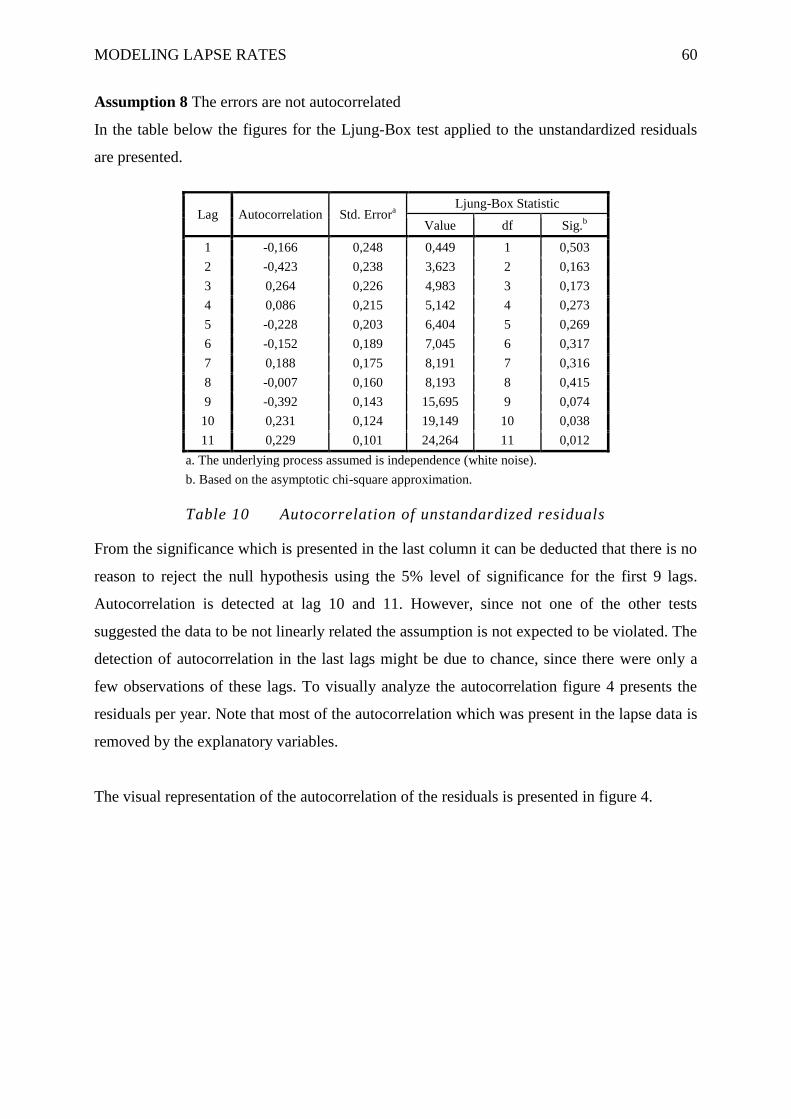
MODELING LAPSE RATES 60
Assumption 8 The errors are not autocorrelated
In the table below the figures for the Ljung-Box test applied to the unstandardized residuals
are presented.
Lag Autocorrelation Std. Errora
Ljung-Box Statistic
Value df Sig.b
1 -0,166 0,248 0,449 1 0,503
2 -0,423 0,238 3,623 2 0,163
3 0,264 0,226 4,983 3 0,173
4 0,086 0,215 5,142 4 0,273
5 -0,228 0,203 6,404 5 0,269
6 -0,152 0,189 7,045 6 0,317
7 0,188 0,175 8,191 7 0,316
8 -0,007 0,160 8,193 8 0,415
9 -0,392 0,143 15,695 9 0,074
10 0,231 0,124 19,149 10 0,038
11 0,229 0,101 24,264 11 0,012
a. The underlying process assumed is independence (white noise).
b. Based on the asymptotic chi-square approximation.
Table 10 Autocorrelation of unstandardized residuals
From the significance which is presented in the last column it can be deducted that there is no
reason to reject the null hypothesis using the 5% level of significance for the first 9 lags.
Autocorrelation is detected at lag 10 and 11. However, since not one of the other tests
suggested the data to be not linearly related the assumption is not expected to be violated. The
detection of autocorrelation in the last lags might be due to chance, since there were only a
few observations of these lags. To visually analyze the autocorrelation figure 4 presents the
residuals per year. Note that most of the autocorrelation which was present in the lapse data is
removed by the explanatory variables.
The visual representation of the autocorrelation of the residuals is presented in figure 4.
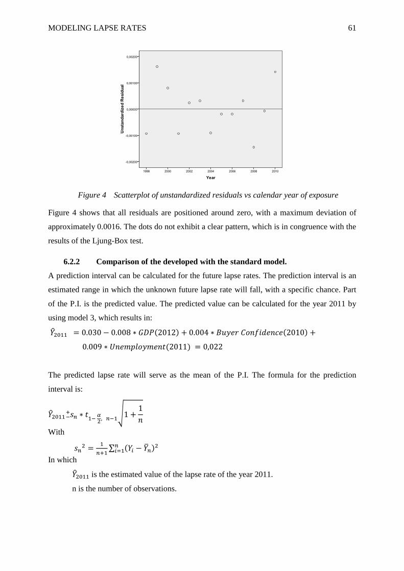
MODELING LAPSE RATES 61
Figure 4 Scatterplot of unstandardized residuals vs calendar year of exposure
Figure 4 shows that all residuals are positioned around zero, with a maximum deviation of
approximately 0.0016. The dots do not exhibit a clear pattern, which is in congruence with the
results of the Ljung-Box test.
6.2.2 Comparison of the developed with the standard model.
A prediction interval can be calculated for the future lapse rates. The prediction interval is an
estimated range in which the unknown future lapse rate will fall, with a specific chance. Part
of the P.I. is the predicted value. The predicted value can be calculated for the year 2011 by
using model 3, which results in:
The predicted lapse rate will serve as the mean of the P.I. The formula for the prediction
interval is:
With
In which
is the estimated value of the lapse rate of the year 2011.
n is the number of observations.
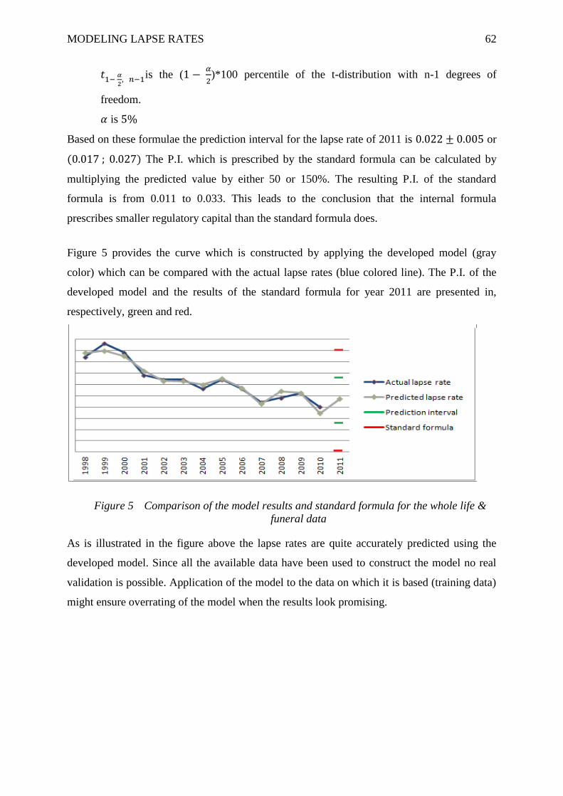
MODELING LAPSE RATES 62
is the (
)*100 percentile of the t-distribution with n-1 degrees of
freedom.
is
Based on these formulae the prediction interval for the lapse rate of 2011 is or
The P.I. which is prescribed by the standard formula can be calculated by
multiplying the predicted value by either 50 or 150%. The resulting P.I. of the standard
formula is from 0.011 to 0.033. This leads to the conclusion that the internal formula
prescribes smaller regulatory capital than the standard formula does.
Figure 5 provides the curve which is constructed by applying the developed model (gray
color) which can be compared with the actual lapse rates (blue colored line). The P.I. of the
developed model and the results of the standard formula for year 2011 are presented in,
respectively, green and red.
Figure 5 Comparison of the model results and standard formula for the whole life &
funeral data
As is illustrated in the figure above the lapse rates are quite accurately predicted using the
developed model. Since all the available data have been used to construct the model no real
validation is possible. Application of the model to the data on which it is based (training data)
might ensure overrating of the model when the results look promising.
19…
19…
20…
20…
20…
20…
20…
20…
20…
20…
20…
20…
20…
20…
Actual lapse rate
Predicted lapse rate
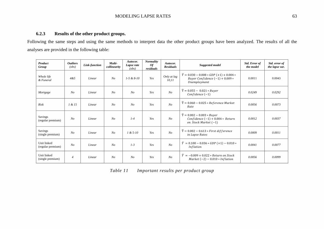
MODELING LAPSE RATES 63
6.2.3 Results of the other product groups.
Following the same steps and using the same methods to interpret data the other product groups have been analyzed. The results of all the
analyses are provided in the following table:
Product
Group
Outliers (obs)
Link-function Multi-
collinearity
Autocor.
Lapse rate
(obs)
Normality
Of
residuals
Autocor.
Residuals Suggested model
Std. Error of
the model
Std. error of
the lapse var.
Whole life
& Funeral 4&5 Linear No 1-5 & 8-10 Yes
Only at lag
10,11
0.0011 0.0043
Mortgage No Linear No No Yes No
0.0249 0.0292
Risk 1 & 15 Linear No No Yes No
0.0056 0.0073
Savings
(regular premium) No Linear No 1-4 Yes No
0.0012 0.0037
Savings
(single premium) No Linear No 1 & 5-10 Yes No
0.0009 0.0011
Unit linked (regular premium)
No Linear No 1-3 Yes No
0.0041 0.0077
Unit linked
(single premium) 4 Linear No No Yes No
0.0056 0.0099
Table 11 Important results per product group
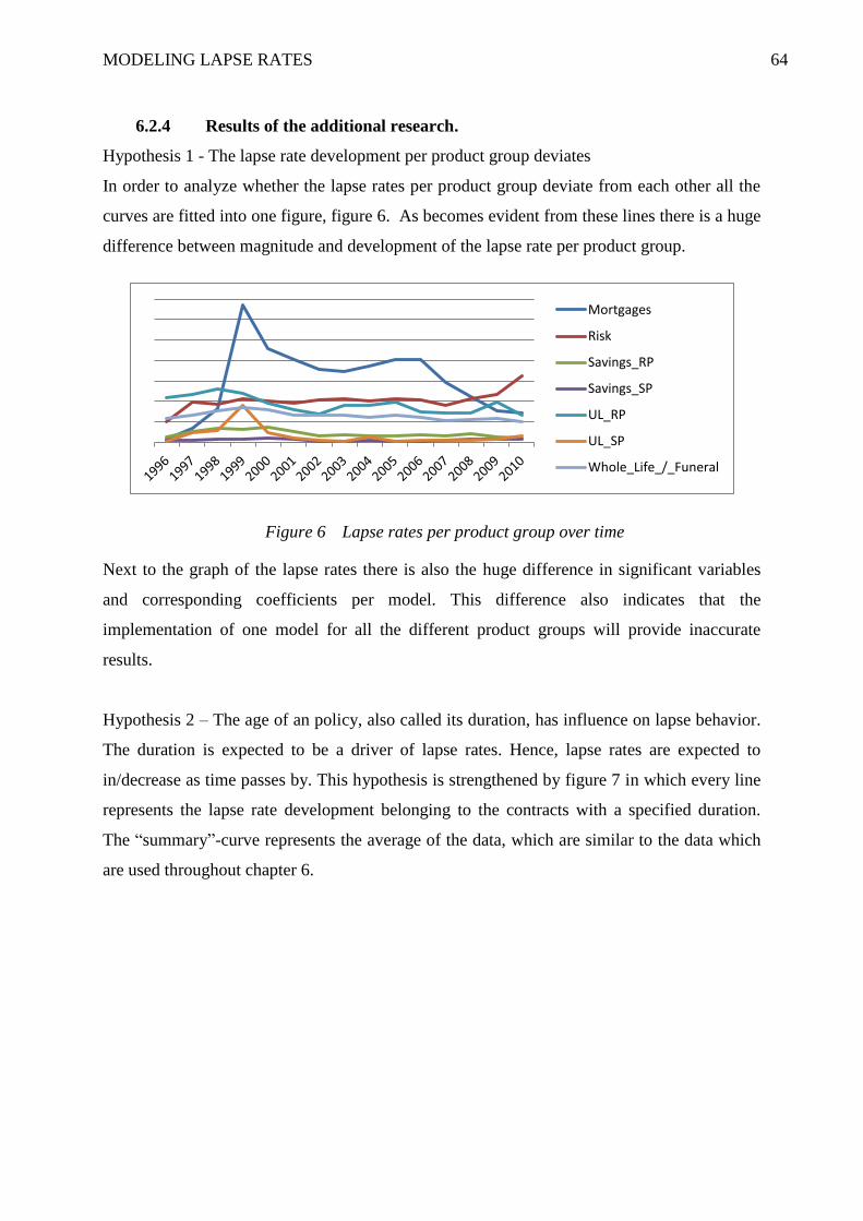
MODELING LAPSE RATES 64
6.2.4 Results of the additional research.
Hypothesis 1 - The lapse rate development per product group deviates
In order to analyze whether the lapse rates per product group deviate from each other all the
curves are fitted into one figure, figure 6. As becomes evident from these lines there is a huge
difference between magnitude and development of the lapse rate per product group.
Figure 6 Lapse rates per product group over time
Next to the graph of the lapse rates there is also the huge difference in significant variables
and corresponding coefficients per model. This difference also indicates that the
implementation of one model for all the different product groups will provide inaccurate
results.
Hypothesis 2 – The age of an policy, also called its duration, has influence on lapse behavior.
The duration is expected to be a driver of lapse rates. Hence, lapse rates are expected to
in/decrease as time passes by. This hypothesis is strengthened by figure 7 in which every line
represents the lapse rate development belonging to the contracts with a specified duration.
The “summary”-curve represents the average of the data, which are similar to the data which
are used throughout chapter 6.
Mortgages
Risk
Savings_RP
Savings_SP
UL_RP
UL_SP
Whole_Life_/_Funeral
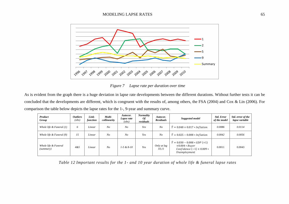
MODELING LAPSE RATES 65
Figure 7 Lapse rate per duration over time
As is evident from the graph there is a huge deviation in lapse rate developments between the different durations. Without further tests it can be
concluded that the developments are different, which is congruent with the results of, among others, the FSA (2004) and Cox & Lin (2006). For
comparison the table below depicts the lapse rates for the 1-, 9-year and summary curve.
Product
Group
Outliers
(obs) Link-
function
Multi-
collinearity
Autocor.
Lapse rate
(obs)
Normality
Of
residuals
Autocor.
Residuals Suggested model
Std. Error
of the model
Std. error of the
lapse variable
Whole life & Funeral (1) 6 Linear No No Yes No 0.0086 0.0114
Whole life & Funeral (9) 15 Linear No No Yes No 0.0042 0.0056
Whole life & Funeral
(summary) 4&5 Linear No 1-5 & 8-10 Yes
Only at lag
10,11
0.0011 0.0043
Table 12 Important results for the 1- and 10 year duration of whole life & funeral lapse rates
1
2
5
9
Summary
MODELING LAPSE RATES 66
When the model is applied to the whole life & funeral lapse data per duration, the first two
cases in table 13, the fit is less accurate than when the average of all durations is modeled. For
that reason, and based on these observations, deviation from the summary model is only
suggested when the lapse rates per duration need to be estimated. The better fit can be caused
by individual behavior which might influence the lapse data per duration while the summary
data are more influenced by macro-economic factors.
Noticeable is that the models for durations 1 and 9 use the same variable, which are different
from those used for the aggregated lapse data. The other remarkable result is that both models
include inflation but with different signs. While an increase in inflation will increase the lapse
rate of products with low durations, it will decrease the lapse rate for products with high
durations.
6.3 Limitations
Although the data set was small there were models, which proved to be significant,
formulized for every product group. These models should be looked upon with caution
for the model might be sensitive to new data.
The generalizability of the models over time and within the company remains
uncertain.
The missing policy data, as is indicated by the statistic and analysis of lapse rate
per policy duration, might help decrease the unexplained variance since the additional
data will increase the number of observations and variables.
The research focused on linear regression models, the appropriateness of this choice
compared to other models has not been analyzed. The small amount of data might
make it impossible to reject other distributions, such as the uniform or exponential
distribution.
MODELING LAPSE RATES 67
Chapter 7 Conclusion and Recommendation
7.1 Conclusion
This thesis started with a research question on explanatory variables and predictive models for
lapse rates in the life insurance industry, which was:
Can the current calculation model for lapse rates be improved41
, while staying in compliance
with the Solvency II directive, and which variables have a significant42
relation to the lapse
rates?
To answer the first part of the question examination had to be done to discover which
predictive models were available as well as applicable to this data set. To answer the second
part of the question it had to be examined which variables could have exercised influence on
the lapse rates, which was tested using data of CBA and FBTO on individually closed
contracts. With the theory in scientific papers as a basis, complemented by company
experience and logic, a list of 38 possible explanatory variables had been composed. The
available data were the aggregated data of CBA and FBTO on a yearly basis from 1996 to
2011.
Literature research on predictive modeling of lapse rates in the insurance industry led to the
choice for predicting with Generalized Linear Models. There are different types of GLMs
with applications dependent on the type and distribution of the included variables. For the
modeling of lapse rates two GLMs are recited. The logistic regression model has been chosen
to model binary lapse data and the linear regression model has been chosen, as a starting
point, for the modeling of continuous lapse data. Application of the linear regression model
provided formulae for forecasting future lapse rates.
A total of 14 variables - including lagged variables, the first difference of lapse rates and
lagged lapse rates – have been analyzed on their relationship with the average lapse rate. Of
these variables “buyer confidence”, “first difference in lapse rates”, “gross domestic product”,
“inflation”, “reference market rate” and “return on stock market” have proven to be valuable
for modeling. Buyer confidence was also of significance in the research of Kiesenbauer
41
The performance of the model has been measured in terms of accuracy, on which it has also been compared.
42 The significance of the variables has been tested by well-chosen statistical measures using a 5% level of
significance.
MODELING LAPSE RATES 68
(2011) which is also one of the only studies which took lagged explanatory variables into
account. The inclusion of reference market rate is analogous to the results of Cox & Lin
(2006) who included the variable complemented by growth in GDP and unemployment in
their predictive model for the aggregated lapse data of the US market. The FSA (2010) stated
that inflation accounted for about 60% of the lapses in their research, which was experienced
to be one of the most significant variables throughout the research. The exclusion of the
binary crises variable indicates that the shocks in 1999 and 2008, if present, were
(significantly) accounted for by the macro-economic variables, analogous to the expectancy
of Kim (2005).
A difference between the developed model and those posted by quoted researchers is in the
number of significant drivers. The general amount of drivers used in literature appeared to be
between 4 and 8, which is quite different from the one or two variable models of this research.
The number of used variables and the r squared statistics were lower than those of Milhaud et
al. (2010) and Briere-Giroux et al. (2010), this indicates that there might be room for
improvement. Although there is room for improvement of the models, every model provides
understandable results and they are all more accurate than the prediction of future lapse rates
by assuming the mean of the lapse data to be a good predictor.
The performance of the model, when compared with the standard formula, is dependent on
the level of expected lapse rates as well as the relative error of the predicted values. The level
of the expected lapse rates greatly influences the standard formula, whereas the relative error
of the predicted values is one of the great contributors to the prediction interval of the
developed model. The influence of the mass lapse event remains unknown and should be
analyzed as well.
Additional research indicated that the assumed difference in lapse rate (development) per
product group is justifiable and that the lapse rate per policy duration deviates in level as well
as in development. These results correspond to those of Cerchiara et al. (2008) who used lapse
data of an Italian banc-assurer of the period 1991 to 2007 and came up with, amongst other
things, policy duration and product class as explanatory variables. They also found
policyholder age and competitiveness of prices to be important, which were not tested. Other
research with congruent results is that of the he FSA (2010) which indicated that a difference
exists between the lapse behavior of contracts with single and regular premiums.

MODELING LAPSE RATES 69
All these findings should be interpreted with caution since assumptions have been made to
justify the applied linear regression model. One of the assumptions which have not been
extensively discussed is that the relations between relevant variables are assumed to remain
existent at future moments. The standard formula avoids this kind of problems since it does
not use any explanatory variables, which is also its weakness. The main difference between
the linear regression model and the time-series model which is in development is in the type
of variables which are included. Whereas the time-series model focuses on past lapse rate
values, the regression model may also includes (future) values of other variables.
7.2 Recommendation
The main limitation of this research was the small amount of data and their level of detail.
Since the results of this research are promising it is recommended to extend the research to
other parts of the company. To increase the statistical strength and accuracy of the inferences
that can be made it is recommended to examine the lapse rates at a policyholder level. This
will provide the option to include more variables in the modeling in order to explain
individual behavior. It should also be verified whether the data are pure and not contaminated,
since some data is expected to be contaminated due to policy mutations (Achmea, 2010b).
The promising results do stimulate monitoring of the model to check its reliability and
accuracy. One of the ways to analyze the model is to compare the results with the time series
model which is under development. If the results are satisfactory it should be investigated
how the model can be implemented in such a way that it fulfills the Solvency II use test.
Finally it should be noted that some confusion about the definition of lapses remains. This is
why it is advised to define and implement a general lapse rate definition to facilitate future
research and minimize the exposure of lapse rates to contamination.
MODELING LAPSE RATES 70
REFERENCES
Achmea (2007). Financial options and guarantees valuation techniques used for embedded
value. Zeist, the Netherlands: Achmea.
Achmea (2010a). Het verhaal van Achlum. Retrieved August 08, 2011, from
http://www.deagendavanachlum.nl/conventie/verhaal/.
Achmea (2010b). Memo: Methodology Lapse Risk – Life (concept). Zeist, the Netherlands:
Achmea.
Anderson, C.J. (2010a). Introduction to Generalized Linear Models (GLMs). Retrieved
October 05, 2011 from http://www.ed.uiuc.edu/courses/edpsy490AT/lectures/4glm1-ha-
online.pdf.
Anderson, C.J. (2010b). Logistic regression for dichotomous responses. Retrieved October
05, 2011 from http://www.ed.uiuc.edu/courses/edpsy490AT/lectures/5logreg-ha-2010-
online.pdf.
Briere-Giroux, G., Huet, J.F., Spaul, R., Staudt, A., & Weinsier, D. (2010). Predictive
modeling for life insurers. Retrieved on October 30, 2011 from
http://www.soa.org/files/pdf/research-pred-mod-life-huet.pdf.
Carson, J.M., & Hoyt, R.E. (1992). An econometric analysis of the demand for life insurance
policy loans. Journal of Risk and Insurance, 59(2), pp. 239-251.
Comité Européen des Assurances [CEA] (2007). CEA - Groupe Consultatif (2007) Solvency
II Glossary. Brussels, Belgium: Comité Européen des Assurances (CEA) and the Groupe
Consultatif Actuariel Européen (Groupe Consultatif).
Committee of European insurance and Occupational Pensions Supervisors[CEIOPS] (2008).
CEIOPS’ Report on its fourth Quantitative Impact Study (QIS4) for Solvency II. Retrieved
August 09, 2011 from https://eiopa.europa.eu/fileadmin/tx_dam/
files/consultations/QIS/CEIOPS-SEC-82-08%20QIS4%20Report.pdf.

MODELING LAPSE RATES 71
CEIOPS (2009). Draft CEIOPS Advice for Level 2 Implementing Measures on Solvency II:
Standard formula SCR - Article 109 c, Life underwriting risk. Retrieved August 09, 2011
from http://www.solvency-ii-association.com/Solvency_ii_Life_Underwriting_Risk.htm.
Centraal Planbureau (2011). Kerngegevens Nederland bijlage 2 cep2011. Retrieved October
30, 2011 from http://www.cpb.nl/sites/default/files/cijfer/Kortetermijnraming%20maart/
april%202011:%20Economie%20groeit,%20maar%20niet%20uitbundig/kerngegevens-
nederland-bijlage-2-cep2011.xls.
Cerchiara, R.R., Edwards, M. & Gambini, A. (2008). Generalized linear models in life
insurance: Decrements and risk factor analysis under Solvency II. Retrieved November 16,
2011 from
http://www.actuaries.org/AFIR/Colloquia/Rome2/Cerchiara_Edwards_Gambini.pdf.
Cox S. H. & Lin Y. (2006). Annuity lapse rate modeling: Tobit or not tobit?. Retrieved
October 30, 2011 http://www.soa.org/files/pdf/Cox%20Linn%20paper%2011-15-06.pdf.
Davis, E.C. (2003). Life Insurance: The origin of premiums, policies and plans. Retrieved
August 08, 2011 from http://ezinearticles.com/?Life-Insurance:--The-Origin-of-Premiums,-
Policies,-and-Plans&id=146330.
Deloitte (2010). Solvency II: Internal model requirements. Retrieved November 16, 2011
from http://www.deloitte.com/assets/Dcom-Belgium/Local%20Assets/Documents/EN/
Services/AERS/Actuarial%20and%20financial%20risk%20advisory/be-aers-fara-solvencyII-
internalmodels_apr2010.pdf.
Doorn, P.K.(2006). Voortgezette Statistiek voor Historici: Multipele regressieanalyse.
Retrieved October 05, 2011 from http://www.let.leidenuniv.nl/history/RES/VStat/
html/les6.html.
EMB Consultancy LLP (2007). Solvency II is based upon three pillars. Retrieved August 09,
2011 from http://www.solvency-2.com/news/threepillars.php.

MODELING LAPSE RATES 72
Eureko Solvency II Project (2009). Solvency II in the pocket. Zeist, the Netherlands: Eureko.
European Central Bank (2007). Potential impact of Solvency II on financial stability.
Frankfurt am Main, Germany: European Central Bank.
European Central Bank (2011). Netherlands – Gross domestic product at market price,
current prices, ECU/Euro, neither seasonally nor working day adjusted, main series.
Retrieved on November 10, 2011 from http://sdw.ecb.int/quickview.do?SERIES_KEY=119
.ESA.A.NL.N.0000.B1QG00.1000.TTTT.V.U.A.
Federal Reserve System (n.d.). Retrieved on October 30, 2011 from
http://www.federalreserve.gov/releases/h15/data.htm#fn1.
Financial Services Authority[FSA] (2004). Stopping short: why do so many consumers stop
contributing to long-term savings policies?. London, England: the Financial Services
Authority.
Fox, J. (2008). Applied regression analysis and Generalized Linear Models. Thousand Oaks,
the United States of America: SAGE Publications, Inc.
FSA (2009a). Insurance Risk Management: The Path to Solvency II, Feedback on DP08/4.
London, England: the Financial Services Authority.
FSA (2009b). Insurance Risk Management: The Path to Solvency II, Discussion paper 08/4.
London, England: the Financial Services Authority.
FSA (2010) 2010 Survey of the persistency of life and pensions policies. London, England:
the Financial Services Authority.
Gate, T. (2000). Normal distribution. Retrieved October 05, 2011 from
http://www.le.ac.uk/bl/gat/virtualfc/Stats/normal.htm.

MODELING LAPSE RATES 73
Grosen, A. & Jørgensen, P.L. (2000). Fair valuation of life insurance liabilities: The impact
of interest rate guarantees, surrender options and bonus policies. Insurance: Mathematics and
Economics, 26; 37-57.
Guszcza, J. (2005). CART from A to B. Retrieved October 30, 2011 from
http://www.casact.org/education/specsem/f2005/handouts/cart.ppt.
Guyon, I. & Elisseeff, A. (2003). An introduction to variable and feature selection. Journal of
Machine Learning Research, volume 3, 1157-1182.
Haberman, S. & Renshaw, A.E. (1986). Statistical analysis of life assurance lapses. Journal
of the Institute of Actuaries, 113, 459-497.
International Centre for Financial Regulation (2009). Solvency II: Summary and update.
Retrieved August 09, 2011 from http://www.icffr.org/getdoc/7b9a0e36-ed23-4129-94c3-
a4a071cd4e06/Misha-Patel---ICFR---Solvency-II-summary-and-updat.aspx.
Investopedia (n.d.). Capital Requirement. Retrieved August 24, 2011 from
http://www.investopedia.com/terms/c/capitalrequirement.asp#axzz1Vpb7Yetb.
Kannan, R., Sarma, K.P., Sarma, S.K. & Rao, A.V. (2008). Lapsation and its impact on
Indian life insurance industry. Retrieved October 30, 2011 from http://www.irdaindia.org/
Final%20Report%20on%20Lapse%20Study.pdf.
Kiesenbauer, D. (2011). Main determinants of lapse in the German life insurance industry.
Retrieved October 30, 2011 from http://www.uni-ulm.de/fileadmin/website_uni_ulm
/mawi/forschung/PreprintServer/2011/Lapse.pdf.
Kim, C. (2005). Modeling surrender and lapse rates with economic variables. North
American Actuarial Journal, 9(4), 56-70.
Kim, C. (2009). Valuing Surrender Options in Korean Interest Indexed Annuities. Asia-
Pacific Journal of Risk and Insurance, 3(2), 46-66.
MODELING LAPSE RATES 74
Kuo, W., Tsai, C., & Chen, W.K. (2003). An empirical study on the lapse rate: the co-
integration approach. Journal of Risk and Insurance, 70(3), 489-508.
Lester, C.E. (1866). The glory and shame of England: Vol. II. The glory and shame of
England. New York, the United States of America: Bartram & Lester.
Loisel, S., Maume-Deschamps, V. & Milhaud, X. (2010). Surrender triggers in life
insurance: Classification and risk predictions. Working paper.
Loisel, S. & Milhaud, X. (2010). From deterministic to stochastic surrender risk models:
Impact of correlation crises on economic capital. European Journal of Operational Research,
Elsevier, 214(2).
Lloyd‟s (n.d.). Key concepts: internal model. Retrieved October 26, 2011 from
www.lloyds.com/the-market/operating-at-lloyds/solvency-II/about/key-concepts.
Michigan state university (2002). Introduction to Person’s r correlation. Retrieved November
16, 2011 from
https://www.msu.edu/~nurse/classes/summer2002/813/week8pearsonrb.htm.
Milevsky, M.A., & Salisbury, T.S. (2002). The real option to lapse and the valuation of
death-protected investments. Retrieved August 24, 2011 from
http://www.ifid.ca/pdf_workingpapers/WP2000B.pdf.
Mun, J. (2010). Modeling risk. Hoboken, the United States of America: John Wiley & Sons,
Inc.
National Institute of Standards and Technology & Sematech. (n.d.). NIST/SEMATECH e-
Handbook of Statistical Methods. Retrieved October 05, 2011 from
www.itl.nist.gov/div898/handbook/.
Nau, R. (2005). Additional notes on regression analysis. Retrieved October 05, 2011 from
htttp://www.duke.edu./~rnau/regnotes.htm.

MODELING LAPSE RATES 75
Nederlandse Zorgautoriteit (2011). Marktscan Zorgverzekeringsmarkt Weergave van de markt
2007-2011. Retrieved August 08, 2011 from
http://www.nza.nl/104107/105773/354532/Marktscan_Zorgverzekeringsmarkt.pdf.
Outreville, J.F. (1990). Whole-life insurance lapse rates and the emergency fund hypothesis.
Insurance: Mathematics and Economics, 9(4), 249-255.
Papps, P.C.H. (1919). A method of estimating the rate of persistency. Record of the American
Institute of Actuaries, 8, 254.
Raghavendra, B.K. & Simha, J.B. (2010). Evaluation of logistic regression model with
feature selection methods on medical dataset. ACS-International Journal on Computational
Intelligence, 1(2).
Robinson, J.J. (2009). The history of life insurance. Retrieved August 08, 2011 from
http://healtharticlescentral.com/the-history-of-life-insurance/.
SAP (n.d.). Adjusted R square. Retrieved October 30, 2011 fromhelp.sap.com/
saphelp_bw21c/helpdata/en/35/e1e6b9e2df0c04e10000009b38f983/content.htm.
Smith, K. (2004). The History of Life Insurance. Retrieved August 08, 2011 from
http://www.financial-shopper-network.com/life_insurance_center.htm.
Solvency II Association (n.d.a). The Minimum Capital Requirement (MCR). Retrieved August
24, 2011 from http://www.minimum-capital-requirement.com/.
Solvency II Association (n.d.b). The Solvency Capital Requirement (SCR). Retrieved August
24, 2011 from http://www.solvency-capital-requirement.com/.
StatSoft (n.d.). Retrieved August 24, 2011 from
http://www.statsoft.com/textbook/classification-and-regression-trees/.

MODELING LAPSE RATES 76
Timofeev, R. (2004). Classification and Regression Trees (CART) Theory and Applications.
Retrieved August 24, 2011 from http://edoc.hu-berlin.de/master/timofeev-roman-2004-12-
20/PDF/timofeev.pdf.
Verbeek, M. (2001). A guide to modern econometrics. Chichester, England: John Wiley &
Sons, ltd.
Wei, W. H. (2002). Outline of generalized linear models. Retrieved October 05, 2011 from
http://web.thu.edu.tw/wenwei/www/glmpdfmargin.htm.
Yaffee, R.A. (2004). Regression analysis with SPSS. Retrieved October 05, 2011 from
http://nyu.edu/its/statistics/publications.html.
Yahoo (n.d.). AEX: Historical Prices. Retrieved October 30, 2011 from
http://finance.yahoo.com/q/hp?s=^AEX&a=09&b=12&c=1995&d=01&e=8&f=2011&g=m.

MODELING LAPSE RATES 77
APPENDICES
Appendix 1: Risk map

MODELING LAPSE RATES 78
Appendix 1: Risk Map
Figure 8 Risk map
In figure 8 most of the (sub-) risk categories which are mentioned in Solvency II and internal
reports are denoted. The tree structure provides a clear example of which variables fall into
which risk category.