Modeling in the Time Domain Introduction - … · Chapter 3 Modeling in the Time Domain Prepared...

Chapter 3 Modeling in the Time Domain

Prepared by: Dr. Mohammad Abdul Mannan of 27

Modeling in the Time Domain

Introduction The state-space approach (also referred to as the modern, or time-domain, approach) is a unified method for modeling, analyzing, and designing a wide range of systems.

The state-space approach can be used to represent nonlinear systems that have backlash, saturation, and dead zone.

It can handle, conveniently, systems with nonzero initial conditions.

Time-varying systems can be represented in state space.

Multiple-input, multiple-output systems can be compactly represented in state space with a model similar in form and complexity to that used for single-input, single-output systems.

It can be used to represent systems with a digital computer in the loop or to model systems for digital simulation. With a simulated system, system response can be obtained for changes in system parameters—an important design tool.

It is also attractive because of the availability of numerous state-space software packages for the personal computer.

While the state-space approach can be applied to a wide range of systems, it is not as intuitive as the classical approach.

The designer has to engage in several calculations before the physical interpretation of the model is apparent, whereas in classical control a few quick calculations or a graphic presentation of data rapidly yields the physical interpretation.

3.2 Some Observations We now demonstrate that for a system (as shown in Figure 3.1) with many variables, such as inductor voltage, vL(t), resistor voltage, vR(t), and capacitor charge, q (t), we need to use differential equations only to solve for a selected subset of system variables because all other remaining system variables can be evaluated algebraically from the variables in the subset. Our examples take the following approach:

1. We select a particular subset of all possible system variables and call the variables in these subset state variables.

2. or an nth-order system, we write n simultaneous, first-order differential equations in terms of the state variables. We call this system of simultaneous differential equations state equations.

3. If we know the initial condition of all of the state variables at t0 as well as the system input for t t0, we can solve the simultaneous differential equations for the state variables for t t0.

4. We algebraically combine the state variables with the system’s input and find all of the other system variables for t t0. We call this algebraic equation the output equation.

5. We consider the state equations and the output equations a viable representation of the system. We call this representation of the system a state-space representation.

Observation with First Order System

Let us now follow these steps through an example. Consider the RL network shown in Figure 3.1 with an initial current of i(0).

1. In this system the variables are i(t), vL(t), and vR(t). We select the current, i(t), for which we will write and solve a differential equation using Laplace transforms.

2. We write the loop equation,



)()()(

tvtRidt

tdiL (3.1)

Figure 3.1 RL network

3. Taking the Laplace transform, using Table 2.2, Item 7, and including the initial conditions, yields

)()()0()( sVsRIissIL (3.2)

Assuming the input, v(t), to be a unit step, u(t), whose Laplace transform is V(s)=1/s, we solve for I(s) and get

)0(1

)( Lis

sIRLs

L

Rs

i

L

Rss

LsI

)0(11

)(

L

Rs

i

L

Rs

sRsI

)0(111

)( (3.3)

from which

tLRtLR eieR

ti )/()/( )0(11

)( (3.4)

The function i(t) is a subset of all possible network variables [i(t), vL(t), and vR(t)] that we are able to find from Eq. (3.4) if we know its initial condition, i(0), and the input, v(t). Thus, i(t) is a state variable, and the differential equation (3.1) is a state equation.

4. We can now solve for all of the other network variables algebraically in terms of i(t) and the applied voltage, v(t). For example, the voltage across the resistor is

tLRtLRR eRietRitv )/()/( )0(1)()( (3.5)

The voltage across the inductor is

)()()()()( tRitvtvtvtv RL (3.6)

The derivative of the current is

)()(1

tRitvLdt

di (3.7)

Thus, knowing the state variable, i(t), and the input, v(t), we can find the value, or state, of any network variable at any time, t t0. Hence, the algebraic equations, Eqs. (3.5) through (3.7), are output equations.



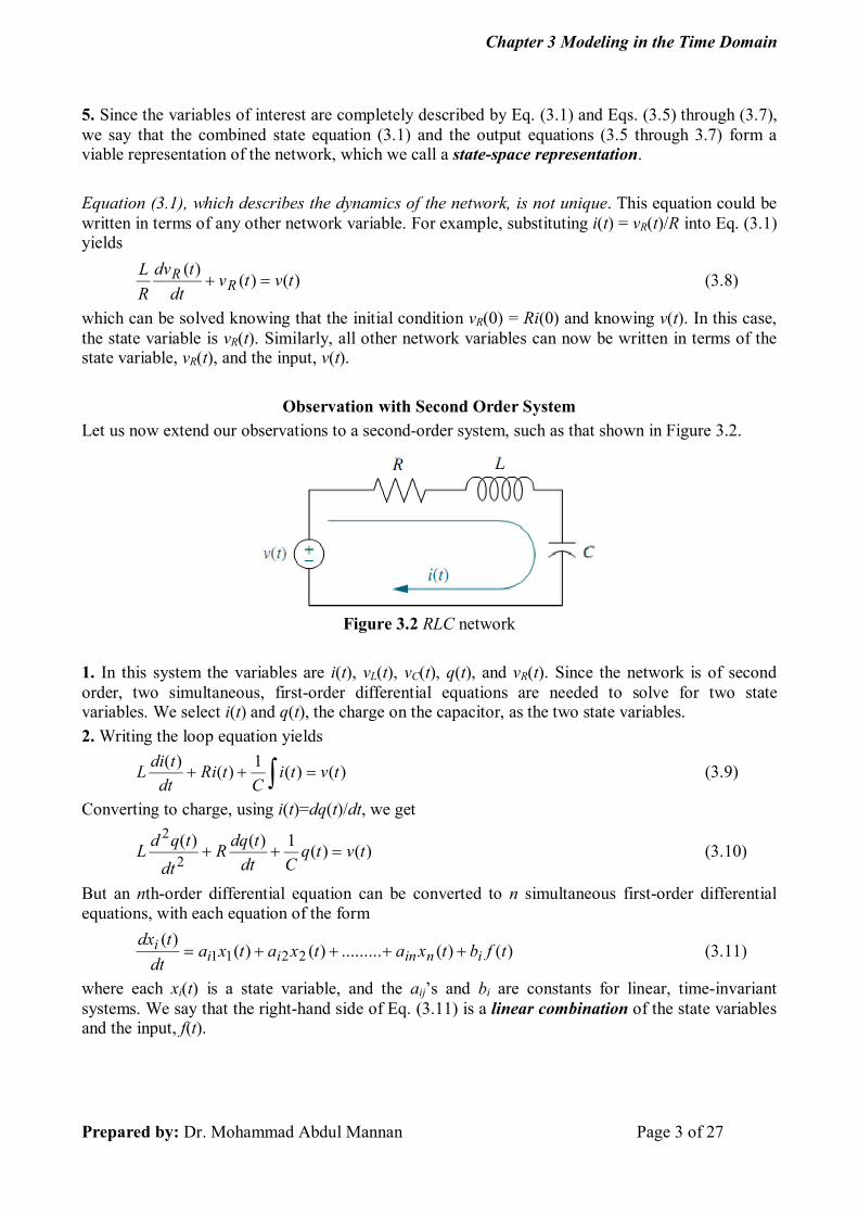
5. Since the variables of interest are completely described by Eq. (3.1) and Eqs. (3.5) through (3.7), we say that the combined state equation (3.1) and the output equations (3.5 through 3.7) form a viable representation of the network, which we call a state-space representation.

Equation (3.1), which describes the dynamics of the network, is not unique. This equation could be written in terms of any other network variable. For example, substituting i(t) = vR(t)/R into Eq. (3.1) yields

)()()(

tvtvdt

tdv

R

LR

R (3.8)

which can be solved knowing that the initial condition vR(0) = Ri(0) and knowing v(t). In this case, the state variable is vR(t). Similarly, all other network variables can now be written in terms of the state variable, vR(t), and the input, v(t).

Observation with Second Order System

Let us now extend our observations to a second-order system, such as that shown in Figure 3.2.

Figure 3.2 RLC network

1. In this system the variables are i(t), vL(t), vC(t), q(t), and vR(t). Since the network is of second order, two simultaneous, first-order differential equations are needed to solve for two state variables. We select i(t) and q(t), the charge on the capacitor, as the two state variables.

2. Writing the loop equation yields

)()(1

)()(

tvtiC

tRidt

tdiL (3.9)

Converting to charge, using i(t)=dq(t)/dt, we get

)()(1)()(

2

2

tvtqCdt

tdqR

dt

tqdL (3.10)

But an nth-order differential equation can be converted to n simultaneous first-order differential equations, with each equation of the form

)()(.........)()()(

2211 tfbtxatxatxadt

tdxininii

i (3.11)

where each xi(t) is a state variable, and the aij’s and bi are constants for linear, time-invariant systems. We say that the right-hand side of Eq. (3.11) is a linear combination of the state variables and the input, f(t).



We can convert Eq. (3.10) into two simultaneous, first-order differential equations in terms of i(t) and q(t). The first equation can be dq(t)/dt=i(t).The second equation can be formed by substituting i(t)dt=q(t) into Eq. (3.9) and solving for di(t)/dt. Summarizing the two resulting equations, we get

)()(

tidt

tdq (3.12a)

)(1

)()(1)(

tvL

tiL

Rtq

LCdt

tdi (3.12b)

3. These equations are the state equations and can be solved simultaneously for the state variables, q(t) and i(t), using the Laplace transform, if we know the initial conditions for q(t) and i(t) and if we know v(t), the input.

4. From these two state variables, we can solve for all other network variables. For example, the voltage across the inductor can be written in terms of the solved state variables and the input as

)(1

)()()( tqC

tRitvtvL (3.13b)

Equation (3.13) is an output equation; we say that vL(t) is a linear combination of the state variables, q(t) and i(t), and the input, v(t).

5. The combined state equations (3.12) and the output equation (3.13b) form a viable representation of the network, which we call a state-space representation.

Another choice of two state variables can be made, for example, vR(t) and vC(t), the resistor and capacitor voltage, respectively. The resulting set of simultaneous, first-order differential equations follows:

)()()()(

tvL

Rtv

L

Rtv

L

R

dt

tdvCR

R (3.14a)

)(1)(

tvRCdt

tdvR

C (3.14b)

Again, these differential equations can be solved for the state variables if we know the initial conditions along with v(t). Further, all other network variables can be found as a linear combination of these state variables.

Is there a restriction on the choice of state variables? Yes! Typically, the minimum number of state variables required to describe a system equals the order of the differential equation. Thus, a second-order system requires a minimum of two state variables to describe it.

We can define more state variables than the minimal set; however, within this minimal set the state variables must be linearly independent. For example, if vR(t) is chosen as a state variable, then i(t) cannot be chosen, because vR(t) can be written as a linear combination of i(t), namely vR(t)=Ri(t). Under these circumstances we say that the state variables are linearly dependent. State variables must be linearly independent; that is, no state variable can be written as a linear combination of the other state variables, or else we would not have enough information to solve for all other system variables, and we could even have trouble writing the simultaneous equations themselves.



The state and output equations can be written in vector-matrix form if the system is linear. Thus, Eq. (3.12), the state equations, can be written as

)()()()(

tttdt

tdBuAxx

x (3.15)

Where,

)(

)()(

ti

tqtx ;

dt

tdidt

tdq

tdt

td)(

)(

)()(

xx

; )()( tvt u ;

L

R

LC

110

A ;

L

10

B

Equation (3.13), the output equation, can be written as

)()()( ttCt Duxy (3.16)

Where, )()( tvt Ly ;

R

C

1C ; 1D

We call the combination of Eqs. (3.15) and (3.16) a state-space representation of the network of Figure 3.2. A state-space representation, therefore, consists of (1) the simultaneous, first-order differential equations from which the state variables can be solved and (2) the algebraic output equation from which all other system variables can be found. A state-space representation is not unique, since a different choice of state variables leads to a different representation of the same system.

3.3 The General State-Space Representation Linear Combination: A linear combination of n variables, xi, for i=1 to n, is given by the following sum, S:

1111 ............ xKXKxKS nnnn (3.17)

Linear Independence: A set of variables is said to be linearly independent if none of the variables can be written as a linear combination of the others. For example, given x1, x2, and x3, if x2=5x1+6x3, then the variables are not linearly independent, since one of them can be written as a linear combination of the other two. Now, what must be true so that one variable cannot be written as a linear combination of the other variables? Consider the example K2x2=K1x1+K3x3. If no xi=0, then any xi can be written as a linear combination of other variables, unless all Ki=0. Formally, then, variables xi, for i=1 to n, are said to be linearly independent if their linear combination, S, equals zero only if every Ki=0 and no xi=0 for all t 0. System Variable: Any variable that responds to an input or initial conditions in a system. State Variables: The smallest set of linearly independent system variables such that the values of the members of the set at time t0 along with known forcing functions completely determine the value of all system variables for all t t0. State Vector: A vector whose elements are the state variables. State Space: The n-dimensional space whose axes are the state variables. State Equations: A set of n simultaneous, first-order differential equations with n variables, where the n variables to be solved are the state variables.



Output Equation: The algebraic equation that expresses the output variables of a system as linear combinations of the state variables and the inputs. Now that the definitions have been formally stated, we define the state-space representation of a system. A system is represented in state space by the following equations:

)()()()(

tttdt

tdBuAxx

x (3.18)

)()()( ttt DuCxy (3.19)

For t t0 and initial conditions. x(t0), where x(t): State vector (xRn i.e. n-dimensional state vector) y(t): Output vector (yRm i.e. m-dimensional output vector) u(t): Input or control vector (uRr i.e. r-dimensional input or control vector) A: System or plant parameter matrix (an nn system or plant parameter matrix) B: Input or control matrix (an nr input or control matrix) C: Output matrix (an mn output parameter matrix) D: Feed forward Matrix (an mr feed forward parameter matrix)

)(

...

...

...

)(

)(

)(

2

1

tx

tx

tx

t

n

x ;

)(

...

...

...

)(

)(

)(

2

1

tu

tu

tu

t

r

u

)(

...

...

...

)(

)(

)(

2

1

ty

ty

ty

t

m

y ;

nnnn

n

n

aaa

aaa

aaa

.......

................

................

.......

.......

21

22221

11211

A ;

nrnn

r

r

bbb

bbb

bbb

.......

................

................

.......

.......

21

22221

11211

B ;

mnmm

n

n

ccc

ccc

ccc

.......

................

................

.......

.......

21

22221

11211

C ;

mrmm

r

r

ddd

ddd

ddd

.......

................

................

.......

.......

21

22221

11211

D

The parameters (elements) aij, bij, cij, and dij of the matrices A, B, C, and D are constant for the linear-time-invariant (LTI) system. If A is a constant parameter matrix and no input is applied (u=0), the state equation represents a homogeneous or autonomous linear system. On the other hand if input is applied (u0), the system is said to be non-homogeneous. Equation (3.18) is called the state equation, and the vector x, the state vector, contains the state variables. Equation (3.18) can be solved for the state variables. Equation (3.19) is called the output equation. This equation is used to calculate any other system variables. This representation of a system provides complete knowledge of all variables of the system at any t t0. Equations (3.18) may be expressed in terms of n first-order differential equations as follows:

)(....)()()(...)()()( 111211111121111 tubtubtubtxatxatxatx rrnn

)(....)()()(...)()()( 212212121221212 tubtubtubtxatxatxatx rrnn

……………… …………….

)(....)()()(...)()()( 12111211 tubtubtubtxatxatxatx rnrnnnnnnnn

The m outputs of the system at time t. may be expressed as linear combination of input and state variables as follows:



)(....)()()(...)()()( 111211111121111 tudtudtudtxctxctxcty rrnn

)(....)()()(...)()()( 212212121221212 tudtudtudtxctxctxcty rrnn

……….. ………..

)(....)()()(...)()()( 12111211 tudtudtudtxctxctxcty rmrmmnmnmmm

The Du(t) in Eq. (3.19) indicates a direct coupling of the input to the output of the system. Since this type of direct coupling of the input to the output is rare, the system may described the following equations:

)()()( ttt BuAxx (3.18a)

)()( tt Cxy (3.19a)

The system (3.18) and (3.19) represent a multi-input and multi-output (MIMO) system. The structure of a MIMO system is shown in the following figure.

Figure Structure of MIMO system.

Often the systems have single-input and single-output (SISO). The state variable representation of SISO system becomes:

)()()( tutt bAxx (3.18b)

)()( tty cx (3.19b)

Where, the input u(t) and output y(t) are scalars, and b and c are n-dimensional vectors. To obtain the internal states, that is the state variables, integrators could be employed in the system structure. The number of integrators involved in the system would be equal to the number of state variables. The time domain state variables representation of a MIMO and SISO system is shown in the following figure.

Why State Variable Approach? An nth order differential equation is not suitable for solution. It is best to obtain a set of n first order differential equations using a set of arbitrary variables called state variables. We need to evaluate the merits of state space approach. The special features of this approach are:

It can handle models both SISO and MIMO in a unified framework. Nonlinear as well as time varying systems can be analyzed conveniently.



The initial conditions can be easily incorporated in the state model, whereas transfer functions are defined for zero initial conditions.

Unlike transfer functions the system model includes the internal states variables as well.

It allows us to design a system with an optimal performance. The state model provides a time domain solution, which is of ultimate interest in

many situations. The state variable formulation in terms of matrix/vector modeling is very efficient

from a computational standpoint. In view of the mathematical elegance also the state variable method has been

adapted for analysis and design.

3.4 Applying the State-Space Representation The first step in representing a system is to select the state vector, which must be chosen according to the following considerations:

1. A minimum number of state variables must be selected as components of the state vector. This minimum number of state variables is sufficient to describe completely the state of the system. 2. The components of the state vector (that is, this minimum number of state variables) must be linearly independent.

Example 3.1: Given the electrical network of Figure 3.5, find a state-space representation if the output is the current through the resistor.

Figure 3.5 Electrical network for representation in state space.

Solution: The following steps will yield a viable representation of the network in state space. Step 1: Label all of the branch currents in the network. These include iL, iR, and iC, as shown in Figure 3.5. Step 2: Select the state variables by writing the derivative equation for all energy-storage elements, that is, the inductor and the capacitor. Thus,

CC i

dt

dvC (3.22)

LL v

dt

diL (3.23)

From Eqs. (3.22) and (3.23), choose the state variables as the quantities that are differentiated, namely vC and iL. Using Eq. (3.20) as a guide, we see that the state-space representation is complete if the right-hand sides of Eqs. (3.22) and (3.23) can be written as linear combinations of the state variables and the input. Since iC and vL are not state variables, our next step is to express iC and vL as linear combinations of



the state variables, vC and iL, and the input, v(t). Step 3: Apply network theory, such as Kirchhoff’s voltage and current laws, to obtain iC and vL in terms of the state variables, vC and iL. At Node 1,

LCLRC ivR

iii 1

(3.24)

which yields iC in terms of the state variables, vC and iL. Around the outer loop,

)(tvvv CL (3.25)

which yields vL in terms of the state variable, vC, and the source, v(t). Step 4: Substitute the results of Eqs. (3.24) and (3.25) into Eqs. (3.22) and (3.23) to obtain the following state equations:

LCC iv

Rdt

dvC

1 (3.26a)

)(tvvdt

diL C

L (3.26b)

or

LCC i

Cv

RCdt

dv 11 (3.27a)

)(11

tvL

vLdt

diC

L (3.27b)

Step 5: Find the output equation. Since the output is iR(t),

CR vR

i1

(3.28)

The final result for the state-space representation is found by representing Eqs. (3.27) and (3.28) in vector-matrix form as follows:

)(10

01

11

tv

Li

v

L

CRCi

v

i

v

dt

d

L

C

L

C

L

C

(3.29a)

L

CR i

v

Ri 0

1 (3.29b)

where the dot indicates differentiation with respect to time. Example 3.2: Find the state and output equations for the electrical network shown in Figure 3.6 if the output vector is y=[vR2 iR2]

T, where T means transpose. Solution: Immediately notice that this network has a voltage-dependent current source. Step 1 Label all of the branch currents on the network, as shown in Figure 3.6. Step 2 Select the state variables by listing the voltage-current relationships for all of the energy-storage elements:

LL v

dt

diL (3.30a)



CC i

dt

dvC (3.30b)

From Eqs. (3.30) select the state variables to be the differentiated variables. Thus, the state variables, x1 and x2, are CL vxix 21 ; (3.31)

Figure 3.6 Electrical network for Example 3.2.

Step 3 Remembering that the form of the state equation is

BuAxx (3.32) we see that the remaining task is to transform the right-hand side of Eq. (3.30) into linear combinations of the state variables and input source current. Using Kirchhoff’s voltage and current laws, we find vL and iC in terms of the state variables and the input current source. Around the mesh containing L and C,

222 Rivvvv RCRCL (3.33)

But at Node 2, LCR vii 42 . Substituting this relationship for iR2 into Eq. (3.33) yields

24 Rvivv LCCL (3.34)

Solving for vL, we get

2241

1Riv

Rv CCL

(3.35)

Notice that since vC is a state variable, we only need to find iC in terms of the state variables. We will then have obtained vL in terms of the state variables. Thus, at Node 1 we can write the sum of the currents as

LL

LR

LRC iR

vtii

R

vtiiitii

11

11

)()()( (3.36)

where vR1=vL. Equations (3.35) and (3.36) are two equations relating vL and iC in terms of the state variables iL and vC. Rewriting Eqs. (3.35) and (3.36), we obtain two simultaneous equations yielding vL and iC as linear combinations of the state variables iL and vC:

CCL viRvR 2241 (3.37a)

)(1

1tiiiv

RLCL (3.37b)

Solving Eq. (3.37) simultaneously for vL and iC yields



)(1

22 tiRviRv CLL

(3.38)

And

)(41

141

12

12 tiRv

RiRi CLC (3.39)

Where

1

2241

R

RR (3.40)

Substituting Eqs. (3.38) and (3.39) into (3.30), simplifying, and writing the result in vector-matrix form renders the following state equation:

)(41141

1

2

2

1

2

2

ti

C

RL

R

v

i

CRC

RLL

R

v

i

C

L

C

L

(3.41)

Step 4 Derive the output equation. Since the specified output variables are vR2 and iR2, we note that around the mesh containing C, L, and R2,

LCR vvv 2

(3.42a)

LCR vii 42

(3.42b)

Substituting Eqs. (3.38) and (3.39) into Eq. (3.42), vR2 and iR2 are obtained as linear combinations of the state variables, iL and vC. In vector-matrix form, the output equation is

)(1411

11 2

1

2

2

2

2 ti

R

v

i

R

R

R

i

v

C

L

R

R

(3.43)

Example 3.3: Find the state equations for the translationalmechanical system shown in Figure 3.7.

Figure 3.7 Translational mechanical system

Solution: First write the differential equations for the network in Figure 3.7, using the methods of Laplace-transformed equations of motion. Next take the inverse Laplace transform of these equations, assuming zero initial conditions, and obtain

0211

21

2

1 KxKxdt

dxD

dt

xdM (3.44)



)(222

2

21 tfKxdt

xdMKx (3.45)

Now let

dt

dv

dt

xd

dt

dv

dt

xdv

dt

dxv

dt

dx 222

21

21

2

22

11 ;;;

and then select x1, v1, x2, and v2 as state variables. Next form two of the state equations by solving Eq. (3.44) for dv1/dt and Eq. (3.45) for dv2/dt. Finally, add dx1/dt= v1 and dx2/dt= v2 to complete the set of state equations. Hence,

11 v

dt

dx (3.46a)

21

11

11

1 xM

Kv

M

Dx

M

K

dt

dv (3.46b)

22 v

dt

dx (3.46c)

)(1

22

21

2

2 tfM

xM

Kx

M

K

dt

dv (3.46d)

In vector-matrix form,

)(

10

0

0

00

1000

0

0010

22

2

1

1

22

111

2

2

1

1

tf

Mv

x

v

x

M

K

M

K

M

K

M

D

M

K

v

x

v

x

(3.47)

where the dot indicates differentiation with respect to time. What is the output equation if the output are x1(t) and x2(t)?

2

2

1

1

2

1

0100

0001

v

x

v

x

x

x (3.47a)

4.10 Laplace Transform Solution of State Equations Taking the Laplace transformation in both-sides Eq. (3.18.1) can be written as follows:

)()()0()( ssss BUAXxX (3.18.1)

Solving Eq. (3.18.7) for X(s), we get

)()0()( 11 ssss -- BUAIxAIX (4.96a)

)()0()( 1 sss - BUxAIX (4.96b)

)()0(det

adj)( s

s

ss BUx

AI

AIX

(4.96c)

x(t) can be obtained by taking inverse Laplace transform of Eq. (3.18.8).



Example 4.11: Given the system represented in state space by Eqs. (4.99),

te

1

0

0

92624

100

010

xx (4.99a)

xy 011 (4.99b)

2

0

1

0x (4.99c)

do the following: (a) Solve the preceding state equation and obtain the output for the given exponential input. (b) Find the eigenvalues and the system poles. Solution: (a) We will solve the problem by finding the component parts of Eq. (4.96), followed by substitution into Eq. (4.97). First obtain A and B by comparing Eq. (4.99a) to Eq. (4.92). Since

92624

10

01

s

s

s

s AI (4.101)

and

2

2

2

231

242624

924

19269

24269

1

sss

sss

sss

ssss AI (4.102)

Since U(s) (the Laplace transform for e-t) is 1=(s + 1); X(s) can be calculated. From Eq. (4.96b) as

1

1

1

0

0

2

0

1

242624

924

19269

24269

1

)(

)(

)(

)(2

2

2

23

3

2

1

ssss

sss

sss

ssssX

sX

sX

sX (4.103)

)4)(3)(2)(1(

293710)(

23

1

ssss

ssssX (4.104a)

)4)(3)(2)(1(

24212)(

2

2

ssss

sssX (4.104b)

)4)(3)(2)(1(

)24212()(

2

3

ssss

ssssX (4.104c)

The output equation is found from Eq. (4.99b). Performing the indicated addition yields



)()(

)(

)(

)(

011)( 21

3

2

1

sXsX

sX

sX

sX

sY

(4.105)

or

4

5.11

3

19

2

5.6

)4)(3)(2)(1(

)51612()(

23

sssssss

ssssY (4.106)

where the pole at -1 canceled a zero at -1. Taking the inverse Laplace transform, ttt eeety 432 5.11195.6)( (4.107)

(b) The denominator of Eq. (4.102), which is det(sI-A), is also the denominator of the system’s transfer function. Thus, det(sI-A)= 0 furnishes both the poles of the system and the eigenvalues: -2, -3, and -4.

4.11 Time Domain Solution of State Equations To solve the differential equation (3.18), we have

)()()( ttt BuAxx (3.18.3)

We now multiply both sides of Eq. (3.18.1) by e-At:

)()()( tetete ttt BuAxx AAA (3.18.4)

We know,

)()( tete

dt

ed ttt

Axxx AA

A

(3.18.5)

From Eqs. (3.18.2) and (3.18.3) we get:

)(tedt

ed tt

Bux A

A

(3.18.6)

Multiplying both sides by dt and integrating between the limits t0 and t, we obtain

t

t

tt detete0

00 )()()( Buxx AAA (3.18.7)

Where the dummy variable has been used in the integral to avoid confusion with t. Solving Eq. (3.18.5) for x(t), we get

t

t

t

t

ttt

dttt

detet

00

00

0

)()()()(

)()()(

Bux

Buxx AA

(4.109)

Where, tet A)( if t0=0, by definition, and which is called the state-transition matrix.

The first term (is called zero input response) on the right-hand-side of Eq. (3.18.6) is seen to be the complementary function or natural response of the system, while the second term (is called convolution integral), which is the convolution integral, is the particular solution or forced response or zero state response. Comparing Eq. (3.18.8) with Eq. (3.18.2), we recognize that e-At is inverse Laplace transform of (sI-A)-1. Similarly, the inverse Laplace transform of the second terms on the right-hand-side of Eq. (3.18.2) is recognized as the convolution integral in Eq. (3.18.8). Since



)(det

adj111 ts

ss -

AI

AIAI LL (4.111)

each term of )(t would be the sum of exponentials generated by the system’s poles.

The initial values of state-transition matrix and its derivative are:

I)0( (4.111.1)

Α)0( (4.111.2)

Example 4.12: For the state equation and initial state vector shown in Eqs. (4.112), where u(t) is a unit step, find the state-transition matrix and then solve for x(t).

)(1

0

68

10tu

xx (4.112a)

0

10x (4.112b)

68

1

68

10

0

0

s

s

s

ss AI

0)4)(2(86det 2 sssss AI from which the poles or eigenvalues are -2 and -4.

Since each term of the state-transition matrix is the sum of responses generated by the poles or eigenvalues, we assume a state-transition matrix of the form:

tttt

tttt

eKeKeKeK

eKeKeKeKt

48

27

46

25

44

23

42

21)( (4.114)

The derivative of state-transition matrix is

tttt

tttt

eKeKeKeK

eKeKeKeKt

48

27

46

25

44

23

42

21

4242

4242)( (4.114.1)

We know,

10

01)0(

8765

4321 IKKKK

KKKK (4.115)

And

68

10

4242

4242)0(

8765

4321 AKKKK

KKKK (4.117)

Comparing both-sides of Eq. (4.115) we have

121 KK (4.116a)

043 KK (4.116b)

065 KK (4.116c)

187 KK (4.116d)

Comparing both-sides of Eq. (4.117) we have



042 21 KK (4.118a)

142 43 KK (4.118b)

842 65 KK (4.118c)

642 87 KK (4.118d)

Solving (4.116a) and (4.118a), we get 1;2 21 KK

Solving (4.116b) and (4.118b), we get 2

1;

2

143 KK

Solving (4.116c) and (4.118c), we get 4;4 65 KK

Solving (4.116d) and (4.118d), we get 2;1 87 KK

Now, we can write

tttt

tttt

eeee

eeeet

4242

4242

2442

1

2

12

)( (4.119)

1

0

2442

1

2

12

)()(4)(2)(4)(2

)(4)(2)(4)(2

tttt

tttt

eeee

eeeet B

)(4)(2

)(4)(2

22

1

2

1

)(

tt

tt

ee

eet B (4.120)

0

1

2442

1

2

12

0)(4242

4242

tttt

tttt

eeee

eeeet x

tt

tt

ee

eet

42

42

44

20)( x (4.121)

tttt

ttttt

deedee

deedeedt

0

44

0

22

0

44

0

22

02

2

1

2

1

)()(

Bu

tt

ttt

ee

eedt

42

42

0

2

1

2

18

1

4

1

8

1

)()( Bu (4.122)

tt

tt

tt

ttt

t ee

ee

ee

eedtttt

42

42

42

42

00

2

1

2

18

1

4

1

8

1

44

2)()()()()( Buxx

tt

tt

ee

eet

42

42

2

7

2

78

7

4

7

8

1

)(x (4.123)



Example 4.13: Find the state-transition matrix of Example 4.12, using (sI-A)-1.

68

1

68

10

0

0

s

s

s

ss AI

from which

4242

842

1

42

6

8

16

86

12

1

ss

s

ss

ssss

s

s

s

sss AI (4.125)

Expanding each term in the matrix on the right by partial fractions yields

4

2

2

1

4

4

2

44

2/1

2

2/1

4

1

2

2

1

ssss

sssss AI (4.126)

Finally, taking the inverse Laplace transform of each term, we obtain

tttt

tttt

eeee

eeeet

4242

4242

2442

1

2

12

)( (4.127)

3.5 Converting a Transfer Function to State Space

Phase Variable Representation It is often convenient to consider the output of the system as one of the state variable and remaining state variable as derivatives of this state variable. The state variables thus obtained from one of the system variables and its (n-1) derivatives, are known as n-dimensional phase variables. Let, the transfer function is given by

011

1

01

1

....

....)(

asasas

bsbsb

sU

sY

sR

sCsG

nn

n

mm

mm

(3.48.1)

(a)

(b)

Figure 3.11.1 Decomposing a transfer function.



We can write Eq. (3.48.1) in the form as

)()()( 21 sGsGsG (3.48.2)

Where,

011

1

111

....

1)(

asasassU

sX

sR

sXsG

nn

n

(3.48.3)

0

11

112 ....)( bsbsb

sX

sY

sX

sCsG m

mm

m (3.48.4)

Eq. (3.48.3) can be written as follows:

sUsXasasas nn

n 101

11 .... (3.48.5)

Taking the inverse Laplace of (3.48.5), we have

tutxadt

da

dt

da

dt

dn

n

nn

n

1011

1

1 ....

tutxa

dt

tdxa

dt

txda

dt

txdn

n

nn

n

101

111

1

11 .... (3.48.6)

Now, let

2

11 x

dt

tdxtx (3.48.7a)

321

22

2 xdt

txd

dt

tdxtx (3.48.7b)

431

33

3 xdt

txd

dt

tdxtx (3.48.7c)

……………………………. ……………………………. …………………………….

121

22

2

nn

nn

n xdt

txd

dt

tdxtx (3.48.7d)

nn

nn

n xdt

txd

dt

tdxtx

11

11

1 (3.48.7e)

n

nn

ndt

txd

dt

tdxtx 1 (3.48.7e)

Using Eq. (3.48.7), the Eq. (3.48.6) can be written as follows:

tutxadt

tdxa

dt

txdatx

n

n

nn

101

111

1

1 ....

tutxatxatxatxatx nnnnn 1021121 .......

tutxatxatxatxatx nnnnn 1122110 ....... (3.48.9)

In vector-matrix form, Eq. (3.48.7) and (3.48.9) become



)(

1

0

....

0

0

0

....

....

10....000

........................

............000

00....100

00....010

....

1

3

2

1

12210

1

3

2

1

tu

x

x

x

x

x

aaaaax

x

x

x

x

n

n

nnn

n

(3.48.10)

Eq. (3.48.4) can be written as follows:

sXbsbsbsbsbsY mm

mm 101

22

11 .... (3.48.11)

Taking the inverse Laplace of (3.48.10), we have

txbdt

db

dt

db

dt

db

dt

dbty

m

m

mm

m

m 1012

2

21

1

1 ....

txbdt

tdxb

dt

txdb

dt

txdb

dt

txdbty

m

m

mm

m

m 101

121

2

211

1

11 ....

(3.48.12)

Using Eq. (3.48.7) we can write Eq. (3.48.11) as

txbtxbtxbtxbtxbty mmmm 10213211 .... (3.48.13)

In vector-matrix form, Eq. (3.48.12) becomes (where, mn)

)(

....

)(

)(

.....

)(

)(

0......)(

1

2

1

110

tx

tx

tx

tx

tx

bbbbty

n

m

mmm (3.48.14)

If the transfer function is given by the following type

011

1

0

....)(

asasas

b

sU

sY

sR

sCsG

nn

n

(3.48.15)

(a)

(b)



Figure 3.11.2 Decomposing a transfer function.

Figure 3.11.2 shows the decomposing of transfer function (3.48.15). According to Figure 3.11.2 and the expressions of Eqs. (3.48.10) and (3.48.14) we have

)(

0

....

0

0

0

....

....

10....000

........................

............000

00....100

00....010

....

0

1

3

2

1

12210

1

3

2

1

tu

bx

x

x

x

x

aaaaax

x

x

x

x

n

n

nnn

n

(3.48.16)

)(

....

)(

)(

.....

)(

)(

0...00...01)(

1

2

1

tx

tx

tx

tx

tx

ty

n

m

m (3.48.17)

Example 3.4: Find the state-space representation in phase-variable form for the transfer function shown in Figure 3.10(a). Solution: Step 1 Find the associated differential equation. Since

24269

24)(

23

ssssU

sY

sR

sCsG (3.54)

cross-multiplying yields

sRsCsss 24)(24269 23 (3.55)

The corresponding differential equation is found by taking the inverse Laplace transform, assuming zero initial conditions:

trtcdt

tdc

dt

tcd

dt

tcd24)(24

)(26

)(9

)(2

2

3

3

(3.56)

Step 2 Select the state variables. Choosing the state variables as successive derivatives, we get

)()(1 tctx (3.57a)

dt

tdctx

)()(2 (3.57b)

2

2

3)(

)(dt

tcdtx (3.57c)



3

33 )()(

dt

tcd

dt

tdx (3.57d)

Differentiating both sides and making use of Eq. (3.57) to find dx1/dt and dx2/dt, and Eq. (3.56) to find d3c/dt3=dx3/dt, we obtain the state equations. Since the output is c=x1, the combined state and output equations are

)()()(

211 txtxdt

tdx (3.58a)

)()()(

322 txtxdt

tdx (3.58b)

)(24)(9)(26)(24)()(

32133 trtxtxtxtxdt

tdx (3.58c)

)(1 txcy (3.58d)

Figure 3.10 (a) Transfer function; (b) equivalent block diagram showing phase variables where

y(t)=c(t). In vector-matrix form,

)(

24

0

0

)(

)(

)(

92624

100

010

)(

)(

)(

3

2

1

3

2

1

tr

tx

tx

tx

tx

tx

tx

(3.59a)

)(

)(

)(

001)(

3

2

1

tx

tx

tx

ty (3.59b)

At this point, we can create an equivalent block diagram of the system of Figure 3.10(a) to help visualize the state variables. We draw three integral blocks as shown in Figure 3.10(b) and label each output as one of the state variables, xi(t), as shown. Since the input to each integrator is xi(t),use Eqs.(3.58a),(3.58b),and(3.58c)to determine the combination of input signals to each integrator. Form and label each input. Finally, use Eq. (3.58d) to form and label the output, y(t)=c(t). The final result of Figure 3.10(b) is a



system equivalent to Figure 3.10(a) that explicitly shows the state variables and gives a vivid picture of the state-space representation. Example 3.5: Find the state-space representation of the transfer function shown in Figure 3.12(a).

Figure 3.12 (a) Transfer function; (b) decomposed transfer function; (c) equivalent block diagram. Where, y(t)=c(t).

Solution: Step 1 Separate the system into two cascaded blocks, as shown in Figure 3.12(b). The first block contains the denominator and the second block contains the numerator. Step 2 Find the state equations for the block containing the denominator. We notice that the first block’s numerator is 1/24 that of Example 3.4. Thus, the state equations are the same except that this system’s input matrix is 1/24 that of Example 3.4. Hence, the state equation is



)(

1

0

0

)(

)(

)(

92624

100

010

)(

)(

)(

3

2

1

3

2

1

tr

tx

tx

tx

tx

tx

tx

(3.63)

Step 3 Introduce the effect of the block with the numerator. The second block of Figure 3.12(b), where b2=1; b1=7, and b0=2, states that

sXsssC 12 27 (3.64)

Taking the inverse Laplace transform with zero initial conditions, we get

txtxtxtc 111 27 (3.65)

But

)()( 21 txtx

)()()( 321 txtxtx

Hence

txtxtxtcty 123 27 (3.66)

Thus, the last box of Figure 3.11(b) ‘‘collects’’ the states and generates the output equation. From Eq. (3.66),

)(

)(

)(

172

3

2

1

tx

tx

tx

ty (3.67)

Although the second block of Figure 3.12(b) shows differentiation, this block was implemented without differentiation because of the partitioning that was applied to the transfer function. The last block simply collected derivatives that were already formed by the first block. Once again we can produce an equivalent block diagram that vividly represents our state-space model. The first block of Figure 3.12(b) is the same as Figure 3.10(a) except for the different constant in the numerator. Thus, in Figure 3.12(c) we reproduce Figure 3.10(b) except for the change in the numerator constant which appears as a change in the input multiplying factor. The second block of Figure 3.12(b) is represented using Eq. (3.66), which forms the output from a linear combination of the state variables, as shown in Figure 3.12(c).

3.6 Converting from State Space to a Transfer Function [Transfer Function from State Equations] The transfer function can be obtained uniquely from the state equations. Taking the Laplace transform of both sides of Eqs. (3.18) and (3.19) with x(0) set equal to zero we get

)()()( sss BUAXsX (3.18.9)

)()()( sss DUCXY (3.19.1)

By solving (3.18.1) we get

)(-)( 1 sss BUAIX (3.18.2)

Substitute Eq. (3.18.2) in the Eq. (3.19.1), we have

)(-)( 1 sss UDBAICY (3.19.2)

The transfer function is now obtained as

DBAICU

Y 1-

)(

)()( s

s

ssG (3.19.3)



Eigenvalues and Transfer Function Poles The expression of (3.19.3) can be written as follows:

)(

)(

-det

-det-adj

-det

-adj)(

sQ

sP

s

ss

s

ssG

AI

AIDBAICD

AI

BAIC (3.19.4)

The denominator polynomial Q(s) is: AI -det)( ssQ (3.19.5)

The polynomial Q(s) is of degree n if A is an nn matrix. Since the poles of the transfer function are the roots of Q(s) and the roots of det(sI-A) are the eigenvalues of A, it is evident that the poles of the transfer function are identical to the eigenvalues of A. The numerator of the transfer function is given by

)(-adj)( sQssP DBAIC (3.19.6)

The degree of the first term in equation (3.19.6) is less than or equal to n-1, while that of the second term will be n, since D is scalar. Hence, the transfer function will always be proper if D is nonzero and will be strictly proper if D=0. Example 3.6: Given the system defined by Eq. (3.74), find the transfer function, T(s) = Y(s)/U(s), where U(s) is the input and Y(s) is the output.

)(

0

0

10

321

100

010

tu

xx (3.74a)

x001ty (3.74b)

Solution:

321

10

01

321

100

010

100

010

001

-

s

s

s

ss AI (3.75)

The denominator polynomial is obtained as

123-det)( 23 sssssQ AI

The adjoint of (sI-A) is obtained as:

2

2

)12(

)3(1

0323

-adj

sss

sss

sss

s AI

The numerator polynomial is obtained as BAIC -adj)( ssP

2310

0

0

10

)12(

)3(1

0323

001)( 2

2

2

ss

sss

sss

sss

sP

The transfer function may now be written as



123

2310

)(

)()(

)(

)()(

23

2

sss

ss

sQ

sPsG

sU

sYsT (3.77)

Example: Determine the transfer function for the following case:

111

021

102

A ;

1

0

1

B ; 112C ; 0D

Solution:

111

021

102

111

021

102

100

010

001

-

s

s

s

ss AI

The denominator polynomial is obtained as

175-det)( 23 sssssQ AI

The adjoint of (sI-A) is obtained as:

4423

1131

2123

-adj2

2

2

ssss

sss

sss

s AI

The numerator polynomial is obtained as

BAIC -adj)( ssP

34

1

0

1

4423

1131

2123

112)( 2

2

2

2

ss

ssss

sss

sss

sP

The transfer function may now be written as

175

34

)(

)()(

23

2

sss

ss

sQ

sPsG

Linearization Example 3.7: First represent the simple pendulum shown in Figure 3.14(a) (which could be a simple model for the leg of the robot shown in Figure 3.13) in state space: Mg is the weight, T is an applied torque in the direction, and L is the length of the pendulum. Assume the mass is evenly distributed, with the center of mass at L/2. Then linearize the state equations about the pendulum’s equilibrium point—the vertical position with zero angular velocity. Solution: First draw a free-body diagram as shown in Figure 3.14(c). Summing the torques, we get

TMgL

dt

dJ

sin

22

2 (3.79)



Where, J is the momment of innertia of the pendulum around the joint of rotation. Select the state variables x1 and x2 as phase variables. Letting

1x

And

11

2 xdt

dx

dt

dx

We write the state equation as

21 xx (3.80a)

J

Tx

J

MgL

dt

dx 12

2

2 sin2

(3.80b)

Thus, we have represented a nonlinear system in state space. It is interesting to note that the nonlinear Eq. (3.80) represent a valid and complete model of the pendulum in state space even under nonzero initial conditions and even if parameters are time varying. However, if we want to apply classical techniques and convert these state equations to a transfer function, we must linearize them.

Figure 3.14 (a) Simple pendulum; (b) force components of Mg; (c) free-body diagram Let us proceed now to linearize the equation about the equilibrium point, x1=0; x2=0, that is, =0 and d/dt=0. Let x1 and x2 be perturbed about the equilibrium point, or

11 0 xx (3.81a)

22 0 xx (3.81a)

Using Eq. (2.182), we have

11011

11

)sin(0sinsin xx

dx

xdx

x

(3.82)

From which

11sin xx (3.83)

Substituting Eqs. (3.81) and (3.83) into Eq. (3.80) yields the following state equations:

21 xx (3.84a)



J

Tx

J

MgLx 12

2 (3.84b)

which are linear and a good approximation to Eq. (3.80) for small excursions away from the equilibrium point. What is the output equation?

References

[1] Norman S. Nise, “Control Systems Engineering,” Sixth Edition, John Wiley and Sons, Inc, 2011.

Modeling in the Time Domain Introduction - … · Chapter 3 Modeling in the Time Domain Prepared...

Documents

Transcript of Modeling in the Time Domain Introduction - … · Chapter 3 Modeling in the Time Domain Prepared...