Modeling Guidelines for Switching Transientsdocshare01.docshare.tips/files/18263/182635568.pdf ·...
24
3-1 Special Publication, Modeling and Simulation Working Group 15.08 Modeling Guidelines for Switching Transients Report Prepared by the Switching Transients Task Force of the IEEE Modeling and Analysis of System Transients Working Group Contributing Members: D.W. Durbak(Co-Chairman), A.M. Gole (Co-Chairman),E.H. Camm, M.Marz, R.C. Degeneff, R.P. O’Leary, R. Natarajan, J.A. Martinez-Velasco, Kai-Chung Lee, A. Morched, R. Sha- nahan, E.R. Pratico, G.C. Thomann, B. Shperling, A. J. F. Keri, D.A. Woodford, L. Rugeles, V. Rashkes, A. Sarshar Abstract - Power Systems Switching Transients are initiated by the action of circuit breakers and switches and by faults. These actions include energization, de-energization, reclosing and fault clearing. The range of frequencies of pri- mary interest in a switching transients study vary from the fun- damental power frequency up to about 10 kHz. Therefore the proper representation must be chosen for the various compo- nents such as transmission lines and cables, transformers, source equivalents, loads and circuit breakers. Equipment mod- eling aspects for the analysis of switching overvoltages are the principal subject of this paper. Keywords : Electromagnetic Transients Simulation, emtp, Switching Transients, Transient Recovery Voltage. 1. INTRODUCTION Switching transients are caused by the operation of breakers and switches in a power system. The switching operations represent two main categories: i) energization phenomena and ii) de-energization of the system elements. The former category include energization of transmission lines or cables, transformers, reactors, capacitor banks etc. The latter category includes fault clearing and load rejections and so on. Due to the complexity of the mathematical repre- sentation of the equipment involved, digital simulation using an electromagnetic transients simulation program plays an important role in the study of switching transients. The results from such studies are useful for: i ) insulation co-ordination to determine overvoltages stresses on equipment ii ) determining the arrester characteristics iii ) determining the transient recovery voltage across circuit breakers. iv ) determining the effectiveness of transient mitigating devices, e.g., pre-insertion resistors, inductors and con- trolled closing devices. The level of detail required in the model varies with the study. For example, a line may be represented by a pi-section equivalent in some line energization studies. In other situations a distributed parameter model with fre- quency dependence may be necessary. In some instances the results are highly sensitive to the value of a certain parameter. For example, the maxi- mum overvoltage for a line energization depends on the exact point on the wave at which the switch contacts close. Thus a number of runs for the same system have to be made with the time of energization being different in each run either in a predictable manner (i.e., for determining the peak overvoltage) or statistically (for obtaining an over- voltage probability distribution). 2. MODELING REQUIREMENTS This section discusses general and specific model- ing requirements. General requirements include a discus- sion of the extent of the system to be modeled, frequency ranges and simulation time-steps. Specific requirements include the equipment models typically used for switching transients simulation. 2.1 TRANSMISSION LINES AND CABLES The most efficient and accurate transmission line models are distributed parameter models based on the trav- elling time τ and characteristic impedance Zc of the line[1,2]. Lumped parameter models (pi-circuits) are com- putationally more expensive (a number of cascaded short- sections are needed to approximate the distributed nature of the physical line) and less accurate. In the phase domain, the current in one phase will cause a voltage in another phase, because of the mutual impedance. In the modal domain, the modes are uncou- pled, and calculations are easier. The transformation between the domains for currents is given by the equation: (1) where [I phase ] is the phase current vector, [ T i ] is [ ] [][ ] e phase I T I i mod ⋅ =
Transcript of Modeling Guidelines for Switching Transientsdocshare01.docshare.tips/files/18263/182635568.pdf ·...
3-1
Special Publication, Modeling and SimulationWorking Group 15.08
Modeling Guidelines for Switching TransientsReport Prepared by the Switching Transients Task Force
of the IEEE Modeling and Analysis of System Transients Working Group
Contributing Members: D.W. Durbak(Co-Chairman), A.M. Gole (Co-Chairman),E.H. Camm, M.Marz, R.C. Degeneff, R.P. O’Leary, R. Natarajan, J.A. Martinez-Velasco, Kai-Chung Lee, A. Morched, R. Sha-nahan, E.R. Pratico, G.C. Thomann, B. Shperling, A. J. F. Keri, D.A. Woodford, L. Rugeles, V. Rashkes,
A. Sarshar
Abstract - Power Systems Switching Transients areinitiated by the action of circuit breakers and switches and byfaults. These actions include energization, de-energization,reclosing and fault clearing. The range of frequencies of pri-mary interest in a switching transients study vary from the fun-damental power frequency up to about 10 kHz. Therefore theproper representation must be chosen for the various compo-nents such as transmission lines and cables, transformers,source equivalents, loads and circuit breakers. Equipment mod-eling aspects for the analysis of switching overvoltages are theprincipal subject of this paper.
Keywords: Electromagnetic Transients Simulation, emtp,Switching Transients, Transient Recovery Voltage.
1. INTRODUCTION
Switching transients are caused by the operation ofbreakers and switches in a power system. The switchingoperations represent two main categories: i) energizationphenomena and ii) de-energization of the system elements.The former category include energization of transmissionlines or cables, transformers, reactors, capacitor banks etc.The latter category includes fault clearing and load rejectionsand so on.
Due to the complexity of the mathematical repre-sentation of the equipment involved, digital simulation usingan electromagnetic transients simulation program plays animportant role in the study of switching transients.
The results from such studies are useful for:i ) insulation co-ordination to determine overvoltages
stresses on equipmentii ) determining the arrester characteristicsiii ) determining the transient recovery voltage across circuit
breakers.iv ) determining the effectiveness of transient mitigating
devices, e.g., pre-insertion resistors, inductors and con-
trolled closing devices.
The level of detail required in the model varieswith the study. For example, a line may be represented by api-section equivalent in some line energization studies. Inother situations a distributed parameter model with fre-quency dependence may be necessary.
In some instances the results are highly sensitiveto the value of a certain parameter. For example, the maxi-mum overvoltage for a line energization depends on theexact point on the wave at which the switch contacts close.Thus a number of runs for the same system have to bemade with the time of energization being different in eachrun either in a predictable manner (i.e., for determining thepeak overvoltage) or statistically (for obtaining an over-voltage probability distribution).
2. MODELING REQUIREMENTS
This section discusses general and specific model-ing requirements. General requirements include a discus-sion of the extent of the system to be modeled, frequencyranges and simulation time-steps. Specific requirementsinclude the equipment models typically used for switchingtransients simulation.
2.1 TRANSMISSION LINES AND CABLES
The most efficient and accurate transmission linemodels are distributed parameter models based on the trav-elling time τ and characteristic impedance Zc of theline[1,2]. Lumped parameter models (pi-circuits) are com-putationally more expensive (a number of cascaded short-sections are needed to approximate the distributed natureof the physical line) and less accurate.
In the phase domain, the current in one phase willcause a voltage in another phase, because of the mutualimpedance. In the modal domain, the modes are uncou-pled, and calculations are easier. The transformationbetween the domains for currents is given by the equation:
(1)
where [Iphase] is the phase current vector, [Ti] is
[ ] [ ] [ ]ephase ITI i mod⋅=
3-2
the transformation matrix, and [Imode] is the modal current
vector. There is a similar expression for voltage, with trans-formation matrix [Tv]. Digital programs only work with real
matrices, so it is helpful if the components of the transforma-tion matrices do not have large imaginary parts. The trans-formation matrix for overhead lines is nearly real, but forcables it may have a significant imaginary part. It is alsosimplest if the transformation matrices are assumed to be fre-quency independent over the range of frequencies found inswitching surges. For overhead lines, the assumption of fre-quency independence can usually be made; for cables thematrices are often frequency dependent. In addition, for pipe-type cables, the cable impedance can be a function of thecable current, if pipe saturation occurs. The saturation is dif-ficult to model.
The distributed parameter model consists of adescription of each mode, and the transformation matrices toreturn to the phase domain. The description of each modewill probably consist of the surge impedance, resistance,velocity and length. More sophisticated frequency depen-dent models will include information on the variation of theparameters with frequency. This may be an important consid-eration when the ground return mode (zero sequence) isinvolved (e.g., during a line to ground fault). In these cases, afrequency dependent distributed parameter line model givesa very accurate representation for a wide range of frequen-cies in the transients phenomenon.The parameters for the dis-tributed parameter model (either frequency-dependent orconstant) are obtained from geometrical and physical infor-mation (line/cable dimensions, height above ground, conduc-tor and soil resistivity) by using a line/cable constantsprogram usually included with the EMTP-type programs
For secondary lines (not directly feeding the phe-nomenon under study), and for those studies where mostlypositive sequence conditions are involved (e.g., three-phaseenergization), a simple distributed constant parameters mod-els can gives satisfactory results.
The use of nominal pi-circuits [1,3] is usuallyrestricted to the case of very short lines when the line’s trav-elling time τ is smaller than the integration step ∆t of the sim-ulation. However, in many instances, cascaded pi-sectionscan be used without excessive loss of accuracy, for studiessuch as line energization [4,5]. The number of pi-circuitsused depends on the desired accuracy, and selecting anappropriate number is important.For overhead lines, theparameters for the pi-section can readily be obtained frompositive and zero sequence fundamental frequency imped-ance values that are used in load flow studies. Typical posi-tive and zero sequence parameters of the overhead lines arepresented in Table 1. The self and mutual impedances to beused in the pi-representation can be obtained using Eqn. 2
(2)
In many cable studies, such as disconnect switchoperation, the constant parameter assumption can be too lim-iting. Here a frequency dependent parameter model must beused, because the frequencies span a large bandwidth and thecable parameters significantly vary within this range. How-ever for solid dielectric cables, the constant parameter modelis often adequate. The calculations shown below are useful indetermining the maximum allowable pi-section length and inestimating errors.
Consider as an example a single phase cable with animpedance of Z per unit length and an admittance Y per unitlength. Then the propagation constant is given by
(3)
and the surge impedance is given by
(4)
Suppose the cable is lossless, and has a total lengthL. Assume each pi-section is used to represent a length (x.The surge impedance for the pi-section is Zo(, given by
(5)
From this expression it is easy to see how small x
Voltage Level
230 kV 345 kV 500 kV 765 kV
Com-ments:
No. of ccts=2Cond/phase=1Gnd. wires=1
ρ=100 Ω-m
No. of ccts=1Cond/phase=2Gnd. wires=2
ρ=100 Ω-m
No. of ccts=1Cond/phase=3Gnd. wires=2
ρ=100 Ω-m
No. of ccts=1Cond/phase=4Gnd. wires=2
ρ=100 Ω-m
X1, Ω/km 0.50 0.38 0.38 0.34
R1, Ω/km 0.052 0.032 0.018 0.017
X0, Ω/km 2.5 1.3 1.2 1.009
R0, Ω/km 0.49 0.341 0.33 0.33
C1, µF/km 0.0088 0.012 0.013 0.013
C0, µF/km 0.0041 0.0083 0.0075 0.0093
Table 1: Typical Transmission Line Parameters at 60 Hz
Xs13--- X0 2X1+( )=
Xm13--- X0 X1–( )=
Cs13--- C0 2C1+( )=
Cm13--- C0 C1–( )=
γ = YZ
Y
ZZo =
( )
∆⋅+≈8
12
xZZ oo
γπ
3-3
has to be for any desired matching of the surge impedance.Next consider the phase error across the length of the cablefor any frequency f. If is the phase shift at any frequency
across one pi-section, then is the phase shift across all N
sections. It can be shown that
(6)
Since the correct phase shift is , the error in the
phase shift can be easily found.
2.2 TRANSFORMERS
For switching surge transient studies, the trans-former model used is a reduced order representation with lessdetail (i.e., as in the example in Fig. 21) in comparison with amodel used for insulation studies. Usually a lumped parame-ter coupled-winding model with a sufficient number of R-L-C elements gives the appropriate impedance characteristics atthe terminal within the frequency range of interest. The non-linear characteristic of the core should usually be included,although the frequency characteristic of the core is oftenignored. This may be an oversimplification as the eddy cur-rent effect prevents the flux from entering the core steel athigh frequencies thereby making the transformer appear to beair-cored. This effect begins to be significant even at frequen-cies in the order of 3-5 kHz.
For swi tch ing surge s tud ies, the fo l lowingapproaches may be used:i ) The model may directly be developed from the trans-
former characteristic e.g., nameplate information or Doble measurements. The standard EMTP models fall into this category. Examples are described in [6,7]
ii ) A model synthesized from measured impedance v/s fre-quency response of the transformer as described in [8,9].This approach is used in the Case Study of section 3.3.5
iii ) A very detailed model obtained from the transformergeometry and material characteristics may be developed.The model is then reduced to one that is usable in thetime domain solution. Examples of this method aredescribed in [7,10,11].
When possible, the following techniques can beused to validate the model. A frequency response obtained bysimulation can be compared within the desired bandwidthwith the actual characteristic if available. This should bedone for all possible open and short circuit conditions on thewindings. Determining the fundamental frequency responsein the form of open and short circuit impedances is a standardcheck. The turns ratio or induced winding voltages at funda-mental frequency are of interest. Comparison with factorytests if available also validates the model. If terminal capaci-
tance measurements are available a comparison betweenmeasured and computed responses is useful.
2.3 SWITCHGEAR
Switchgear includes circuit breakers, circuit-switchers, vacuum switches and other devices which make orbreak circuits. In switching surge studies, the switch is oftenmodeled as an ideal conductor (zero impedance) whenclosed, and an open circuit (infinite impedance) when open.Transient programs allow various options to vary the closingtime ranging from one-shot deterministic closings to multi-shot statistical or systematic closings.
Statistical Switching: Transient voltage and current magni-tudes depend upon the instant on the voltage waveform atwhich the circuit breaker contacts close electrically [12]. Astatistical switching case typically consists of 100 or moreseparate simulations, each using a different set of circuitbreaker closing times. Statistical methods can be used to pro-cess the peak overvoltages from each simulation. Fig. 1 is aplot derived from 100 peak overvoltage magnitudes from theline energization case study presented in section III A. Thisplot shows a 10% probability (Y axis) of exceeding 2 pu volt-age (X axis).
Circuit breakers can close at any time (angle) on thepower frequency wave. For a single phase circuit, the set ofcircuit breaker closing times can be represented as a uniformdistribution from 0 to 360 degrees with reference to thepower frequency. The standard deviation for a uniform distri-
bution over 1 cycle is , where f is the frequency ofthe waveform.
A three phase (pole) circuit breaker can be modeledas three single phase circuit breakers, each with independentuniform distributions covering 360 degrees. However, analternative (dependent) model can be used if the three polesare mechanically linked and adjusted so that each poleattempts to close at the same instant. In reality, there will be afinite time or pole span between the closing instants of thethree poles. The pole span can be modeled with an additionalstatistical parameter, typically from a Gaussian (normal) dis-tribution. For a mechanically linked three pole circuitbreaker, the closing times use both uniform distributionparameters and Gaussian distribution parameters. All threedependent poles use the same parameter from the uniformdistribution, which varies from 0 to 360 degrees. Each poleuses a unique parameter from the Gaussian distribution. Thestandard deviation of the maximum pole span is typically 17to 25 percent of the maximum pole span. For the case studyin section III A, a maximum pole span of 5 ms was assumed.
Statistical cases with pre-insertion resistors or reac-tors require a second set of three phase switches. The first setis modeled as described above. The closing times of the sec-
γn
γnN
( )2
332
2424 N
LL
xLLN
γγγγγγ π −⋅=∆⋅⋅⋅
−⋅≈
γL
1 2 3f( )⁄

3-4
ond set (which shorts the resistors or reactors) are dependentupon the first set plus a fixed time delay, typically one-half toone cycle for pre-insertion resistors used with circuit break-ers, and 7 to 12 cycles (depending on application voltageclass) for pre-insertion reactors used with circuit-switchersclosing in air through high-speed disconnect blades.
Fig. 1. Overvoltage Distribution Probability
Pre-Striking: In the model described above, a normal distri-bution was assumed for the closing of the phase switches. Inreality, the withstand strength of the contacts decreases as thecontacts come closer. When the field stress across the con-tacts exceeds this withstand strength, pre-strike occurs. If thisis taken into account, the distribution of closing angles isconfined to the rising and peak portions of the voltage wave-shapes [13].
Some modern devices can control the closing angleof the poles to close at or near the voltage zero between thecontacts. Such devices are being applied to capacitor bankswitching and can reduce overvoltages and inrush currents.For such devices, the maximum angle in the tolerance of thevoltage zero closing control should be used. Alternatively, astatistical switching method can be applied to the breakerpoles over the time span around the voltage zero, within thetolerance of the closing time [13].
Opening: Typical transient studies require the switch to openat a current zero. The dynamic characteristic of the arc is usu-ally not important and is not modeled in most cases. How-ever, in certain instances where small inductive currents arebeing interrupted, the current in the switch can extinguishprior to its natural zero crossing. Severe voltage oscillationscan result due to this current-chopping that can stress the cir-cuit breaker. Modeling of this phenomenon is described inadditional detail in available literature [14,15] and is not cov-ered here
In cases of current chopping, an arc model may benecessary. A good description of the methodology is avail-able in [16].
Faults: Faults are usually modeled as ideal switches in serieswith other series elements if necessary. The switch can beclosed during the steady state solution or closed at a specifictime or voltage. Several runs with variations in the closinginstant should be carried out as the point on wave of switch-ing can affect the transient.
Sometimes faults are modeled with flashover con-trolled switches to represent a gap. The switch is operatedtypically, when the gap voltage exceeds a fixed value. Moresophisticated models include a volt-time characteristic.
Faults generally involve arcs. Arcs can be modeledby various approximations such as:i ) Ideal Switch (R= 0, V =0)ii ) Linear resistance R or constant voltage Viii ) Constant V and series Riv ) Series V and R that vary according to some assumed
functionv ) V and/or R that vary according to some differential
equation [17].
The most commonly used option is i) above as thearc voltage is usually small compared with voltage dropselsewhere (i.e., along the transmission line). Arc modelingcan be important when studying secondary arc phenomena,such as single pole reclosing. Discussion on the modeling ofthis phenomenon is available in the literature[18].
2.4 CAPACITORS AND REACTORS
Capacitor banks are usually modeled as a singlelumped element. However, some switching transient simula-tions require the modeling of secondary parameters such asseries inductance and loss resistance. The inductance of thebuswork is sometimes important when studying the back toback switching of capacitor banks, or in the study of faults onthe capacitance bus. The damping resistance of this induc-tance should be estimated for the natural frequency of oscil-lations.
Reactors are modeled in many studies by a simplelumped inductor with a series resistance. A parallel resis-tance may be added for realistic high frequency damping.Core saturation characteristic may also have to be modeled.A parallel capacitance across the reactor should be includedfor reactor opening studies (chopping of small currents). Thetotal capacitance includes the bushing capacitance and theequivalent winding to ground capacitance. For series reac-tors, there is a capacitance from the terminal to ground andfrom terminal to terminal.

3-5
2.5 SURGE ARRESTERS
Gapless metal oxide surge arresters are character-ized with a nonlinear voltage versus resistance characteristic.Two model types are used frequently in EMTP-type studies[19]. The pseudo non-linear model, while easy to set up, cancause computational problems with the solution as the char-acteristic can only change at the end of every time-step. Thepreferred model is a true non-linear element which iterates ateach time-step to a convergent solution and is thus numeri-cally robust. The V-I characteristic, usually determined fromthe 36 x 90 µs surge should be modeled with 5-10 (preferablyexponential as opposed to linear) segments.
Waveshape dependent characteristics are usually notrequired for most switching transient simulations. Likewise,the surge arrester lead lengths and separation effects can alsobe ignored for such studies. Modeling of the older seriesgapped SiC arresters is not discussed in this paper.
2.6 LOADS
Power system loads are mostly resistive, indicativeof heating and lighting loads, and the active component ofmotor loads. The reactive components of motor and fluores-cent lighting loads are the other major contributors to powersystem loads. In general, the power system load is repre-sented using an equivalent circuit with parallel-connectedresistive and inductive elements. The power factor of theload determines the relative impedance of the resistive andinductive elements. Shunt capacitance is represented with theresistive and inductive elements of the load if power-factorcorrection capacitors are used. Whenever loads are lumped ata load bus, the effects of lines, cables, and any transformersdownstream from the load bus need to be considered [5].This is particularly important for the modeling of high-fre-quency transient phenomena. In such cases, an impedance Zs
in series with the parallel R-L-C load equivalent circuit isappropriate as shown in Fig. 2. The series impedance, com-bined with the equivalent source impedance at the load bus,is typically in the range of 10 to 20 percent of the load imped-ance.
Certain types of load, e.g., large motor loads, elec-tronic loads, or fluorescent lighting loads, may require spe-cif ic representation of certain load components (e.g.induction motors, adjustable-speed drives, power supplies,etc.). The need for such detailed representation will be deter-mined by the phenomenon being investigated.
Actual power system loads are distributed through-out the system. Some concentration of loads occur in certainareas. Loads close to the substation can be lumped. Distantloads can be lumped based on load concentration and repre-sented along lines or distribution feeders described by suit-able line or cable models.
Fig. 2. Equivalent circuit representation of power system loads for simulating switching transients
2.7 SOURCES AND NETWORK EQUIVALENTS
In switching transient studies, the source is modeledas an ideal sine-wave source. Generators are modeled as avoltage behind a (subtransient) Thevenin impedance. Often anetwork equivalent is used in order to simplify the represen-tation of the portion of the power network not under study.Some typical network equivalents are shown in Fig. 3
Fig. 3. Conventional Network Equivalents
The first type a) represents the short circuit imped-ance (Thevenin equivalent) of the connected system. The X/R ratio is selected to represent the damping (the damping
angle is usually in the range 75o-85o). The second type b)represents the surge impedance of connected lines. Thisequivalent may be used to reduce connected lines to a simpleequivalent surge impedance and where the lines are longenough so that reflections are not of concern in the systemunder study. If the connected system consists of a knownThevenin equivalent and additional transmission lines, thetwo impedances may be combined in parallel in the mannerof Fig. 3c. It should be noted however, that this approachmay yield an incorrect steady-state solution if the equivalentimpedance of the parallel connected lines is of comparable
IL
RL
Load busVll
X
LX XC
ZS
RS
S
Xsc Rsc
Xsc Rsc
Zsc
Zsc
a) Short Circuit Impedance
c) Short Circuit Impedance + Surge Impedance
b) Surge Impedance

3-6
magnitude to the source impedance. In such a case it may notbe possible to lump the source and lines into one equivalentimpedance.
More complex equivalents which properly representthe frequency response characteristic (as opposed to the onesabove that are most accurate near fundamental frequency) arealso possible [20,21]. Mutually-coupled sources are oftentypical for line-fed substations.
2.8 TIME-STEP AND SIMULATION LENGTHS
The time step to be chosen should be small enoughto properly represent the smallest time constant in the mod-eled system. It should also be significantly smaller (typically1/20 th) than the period of the highest frequency oscillatorycomponent. Additional factors that affect the time-step arethe presence of non-linear characteristics such as arrestercharacteristics, and the minimum travel time of travellingwave cable and transmission line models. Time-steps in therange of 5 µs to 50 µs (typically 20 µs) are used. The simula-tion time in typical switching surge studies ranges from 20ms to 200 ms (typically 50 ms). Slightly larger time-steps (20µs-50 µs) can be used with programs that use interpola-tion[22], because the linear interpolation method calls forless iteration of surge arrester characteristics and also doesnot introduce spurious current chopping.
One simple method for checking the suitable time-step is to check if no further gains in accuracy accrue fromany further time-step reduction.
3. CASE STUDIES
Typical case studies are now presented for a practi-cal demonstration of the modeling guidelines. Several differ-ent examples are considered: Line energization, transientrecovery voltage determination for line and transformerfaults and the switching of shunt as well as series capacitorbanks.
3.1 LINE ENERGIZATION
Aim: The aim of such a study is to determine the overvoltagestresses and choose the insulation strength in order to achievean outage rate criterion [23].
3.1.1 Phenomena:
The energization of overhead transmission lines by closingthe circuit breaker produces significant transients. It isimportant to distinguish between two closely related phe-nomena: energization and reclosing. In the former case, thereis no trapped charge. In the latter case of reclosing, the linemay have been left with a trapped charge after the initialbreaker opening. In this case, the transient overvoltages canreach higher values (up to 4.0 pu).
3.1.2 Model
The source, transformer, overhead lines, circuit breaker andthe trapped charges (if any) on the line are to be modeled inorder to study the line energization transients. In this study asimple power system is used to demonstrate the simulationresults.
The network configuration of a 345 kV circuit isshown in Fig. 4. The 345 kV source (1 pu) is connectedthrough a transformer to the 203 km overhead line. The linewas modeled with several pi-sections in the mannerdescribed in section 2.2.1.The parameters are given at 60 Hzas:
Source and transformer impedance, Z1 = Z0 = (6.75 + j127)ΩLine impedance, Z1 = (0.04+j0.318) Ω/km
Line impedance, Z0 = (0.26+j1.015) Ω/kmCharging capacitance, C1 = 11.86 nF/km
Charging capacitance, C0 = 7.66 nF/km
Fig. 4. One Line Diagram of System Used for Energization Study
3.1.3 Simulation Results
First a statistical overvoltage study is conducted in order toevaluate the switching time at which maximum transients areproduced. The results of the statistical energization studywere presented in Fig. 1. Then the effect of various parame-ters and related issues on the energization transients are stud-ied.
Four, eight or sixteen pi-sections gave similarresults although the maximum overvoltage was slightlyhigher with eight pi-sections. No significant improvementwas obtained by reducing the time-step below 50 µs.
The overvoltages produced in the presence oftrapped charge on the line depend on the polarity and themagnitude of the trapped charges. Therefore additional stud-ies were carried out to see the effect of trapped charge on theline. For reclosure operations, it is assumed that trappedcharges on phases A, B, and C are -0.9, -0.8, and 0.8 per unitrespectively.
CB
Source (1 pu, 60Hz)203 km transmission line
TR TR - TransformerCB- Circuit breaker

3-7
From Table 2 it can be seen that the highest over-voltage magnitude due to the presence of trapped charges is2.839 pu. The corresponding overvoltage magnitude in theabsence of trapped charges are 2.2 pu (Fig. 1). Typical ener-gization waveforms are shown in Fig. 5.
Additional studies (not shown) that can be con-ducted on this model include the comparison of simultaneousand non-simultaneous closing of breaker contacts, the effectof including a closing resistance and including the effect onsurge arrester ratings.
Fig. 5. Voltage At Open End Of Line on Energization with Trapped Charge
3.2 ENERGIZATION OF PIPE-TYPE CABLE
Aim: To determine the maximum overvoltages in the cable.
3.2.1 Phenomena
As in the case of overhead transmission line energization, theovervoltage in the cable is a function of the point on wave of
the switching instant. The peak overvoltages are then deter-mined using statistical switching.
3.2.2 Model
The first example that was done was a 345 kV pipe-type(HPFF or high pressure fluid filled ) cable. A drawing of thecable is shown in Fig. 6. The 345 kV cable has 2500 kcmilsegmented conductors with a 1.824 inch diameter, 1.035 inchof paper insulation with a dielectric constant ε = 3.5. Thesheath is 0.01 inch.
Fig. 6. Geometry of HPFF cable example.
thick, and the sheath resistivity was set to ρ = 1.0x10⁻⁵ Ωm toaccount for the wrapping pitch. A 10.5 inch pipe with a 0.25
inch wall thickness was used; for the pipe a ρ = 14x10-8 Ωmwas used. It was assumed that all shields and the pipe werecontinuously grounded.
The cable was energized using the simple powersystem, shown in Fig. 7. The energizing was done with avariety of cable models, including traveling wave and pi-cir-cuit models. A decision must be made about the number ofpi-sections to be used in the model, and the equations fromthe preceding section can assist in making the choice. Forthe pipe-type cable, the positive sequence propagation con-
stant is γ1~ 3.75x10⁻³/km, and the zero sequence propagation
constant is γ0 ~ 7.28x10⁻³/km. Based on these values, for thesurge impedance of the pi-circuit to be within 10% of the cor-rect value, the pi-circuit section lengths must be less than 239km based on positive sequence parameters and less than 123km based on zero sequence. Therefore, the surge impedancerequirements have little impact on the pi-section length forthis short cable. Next, suppose it was desired that the oneway phase shift error be less than one radian at a frequency of900 Hz. Then, based on the positive sequence parameters 14pi-sections would be required for the 20 km cable. For thezero sequence parameters, 38 pi-sections would be requiredfor this same phase error! A 15 section model was actually
Location Phase A pu
Phase B pu
Phase C pu
Source end 1.272 2.164 2.413
Open end 1.442 2.839 2.784
Table 2: Overvoltages in the Presence of Trapped Charge

3-8
used. In addition, a 3 section model was used to see theeffect of using only a small number of sections.
Fig. 7. Simple power system for cable energizing.
Table 3: Maximum switching surges in pu at each end of the cable.
3.2.3 Simulation Results
The cable was energized with no reactors installed,to eliminate the influence of other equipment. A statisticalsimulation was conducted, consisting of 100 energizations,using a breaker with a 6 ms pole span and no insertion resis-tors. The maximum overvoltages obtained are shown inTable 3 for several cable models. The breaker pole closingtimes that gave the maximum voltage at the open end of thecable for the 60 Hz traveling wave model were then selected,and deterministic simulations were run using these closingtimes. Three simulations were done, using the 60 Hz travel-ing wave model, the 15 section 60 Hz pi model, and the 3section 60 Hz pi model. Plots of the voltage at the open cableend are shown in Fig. 8.
The deterministic simulations were then repeatedusing cable models evaluated at 1000 Hz. The results areshown in Fig. 9. As can be seen from the table, there is littledifference in the maximum switching surge for any of the 60Hz models. It appears that either the traveling wave model orpi- circuit model can be used to obtain a switching surge dis-tribution when the cable is energized. The results for the1000 Hz model are also consistent, but the values obtainedwith the 1000 Hz models are considerably smaller than thoseobtained with the 60 Hz models. Therefore, it would appearto be advisable to use a frequency dependent cable model if itis available.
Fig. 8. Switching surge overvoltage using 60 Hz models. Traveling wave model (top), 15 pi-section model (middle), 3 pi-section model (bottom).
Fig. 9. Switching surge overvoltage using 1000 Hz models. Traveling wave model (top), 15 pi-section model (middle), 3 pi-section model (bottom)
3.3 ENERGIZATION OF A SOLID DIELECTRIC CABLE
Aim: As in the previous section, the aim of this study is todetermine the maximum overvoltages in the cable resultingfrom energization. The effect of using different cable model-ling options such as various numbers of pi-section or distrib-uted parameters is also presented.
Cable Model H IN H OUT
Traveling wave model with 60Hz parameters
2.30 2.35
15 section pi-circuit model with60 Hz parameters
2.30 2.40
3 section pi-circuit model with60 Hz parameters
2.25 2.35
Traveling wave model with1000 Hz parameters
2.05 2.10
15 section pi-circuit model with1000 Hz parameters
2.05 2.10
3-9
3.3.1 Phenomena
Eddy current losses in the iron pipe around the cables in anHPFF system discussed above would have considerableeffect on the switching surges, resulting in lower overvolt-ages as compared to those for the solid dielectric cables.Therefore, another example was done using a 138 kV soliddielectric (SD) cable.
3.3.2 Model
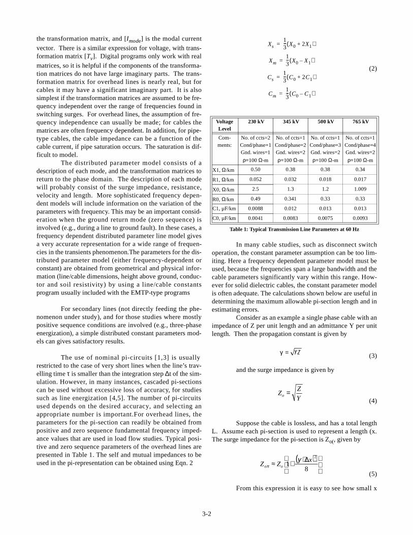
A 138 kV solid dielectric cable with the geometryshown in Fig. 10 was modelled.
The three cables were installed 1.2 m undergroundwith a 25 cm horizontal spacing between the conductors.The lead sheath was grounded at only one end, and thesheaths were crossbonded at 1000 m intervals.
Fig. 10. 138 kV SD cable.
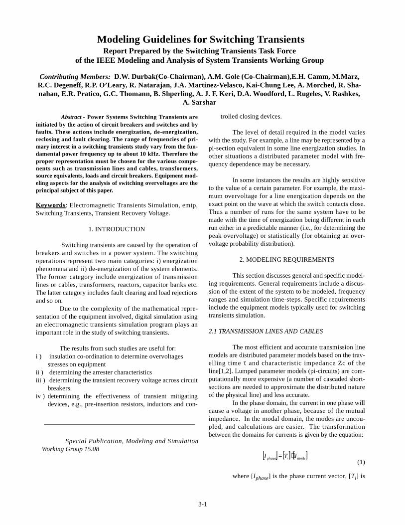
The circuit for energizing the 138 kV cable wasapproximately the same as used for the 345 kV HPFF cable,except of course the voltage levels had to be changed, andsome changes had to be made in the equipment. A typical138 kV compact design overhead line was used, and theautotransformer was turned around, with 230 kV used for thehigh side transformer voltage. The transformer size was alsoreduced to 100 MVA A sketch of the energizing circuit isshown in Fig. 11. In the several cases simulated, various dif-ferent models, pi-section as well as distributed parametermodels were used for the cable.
3.3.3 Simulation Results
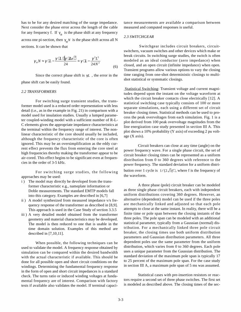
A series of statistical energizing simulations weredone, and the maximum overvoltages are shown in Table 4.As can be seen, the values obtained with the 60 Hz modelsare very close to each other. The 1000 Hz values are alsoconsistent, and, unlike the HPFF cable, the 1000 Hz valuesare very close to those obtained at 60 Hz. Therefore, the fre-quency dependent model may not be necessary for the SDcable.
Fig. 11. Simple circuit used for energizing 138 kV cable.
Table 4: Overvoltages when 138 kV cross bonded cable is energized.
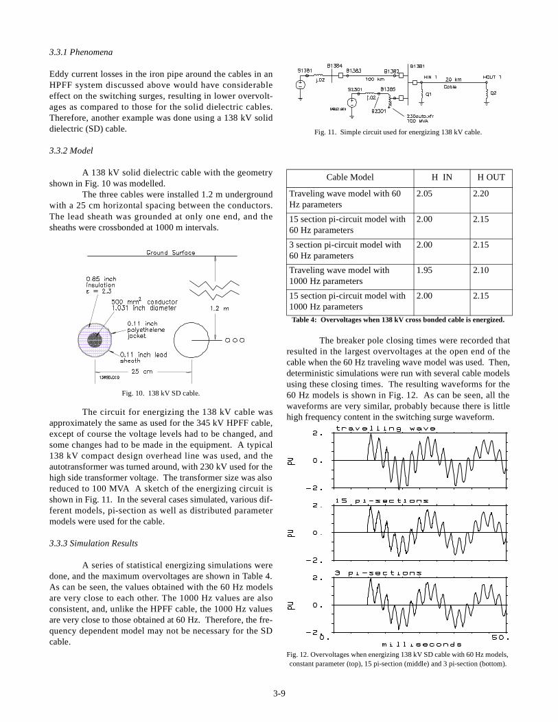
The breaker pole closing times were recorded thatresulted in the largest overvoltages at the open end of thecable when the 60 Hz traveling wave model was used. Then,deterministic simulations were run with several cable modelsusing these closing times. The resulting waveforms for the60 Hz models is shown in Fig. 12. As can be seen, all thewaveforms are very similar, probably because there is littlehigh frequency content in the switching surge waveform.
Fig. 12. Overvoltages when energizing 138 kV SD cable with 60 Hz models, constant parameter (top), 15 pi-section (middle) and 3 pi-section (bottom).
Cable Model H IN H OUT
Traveling wave model with 60 Hz parameters
2.05 2.20
15 section pi-circuit model with 60 Hz parameters
2.00 2.15
3 section pi-circuit model with 60 Hz parameters
2.00 2.15
Traveling wave model with 1000 Hz parameters
1.95 2.10
15 section pi-circuit model with 1000 Hz parameters
2.00 2.15

3-10
The deterministic simulations were then rerun usingthe 1000 Hz cable models. The results are shown in Fig. 13.As can be seen, for the SD cable there is not as much differ-ence between the 60 Hz and 1000 Hz results as there was forthe pipe-type cable. Again, this would seem to indicate thatthe frequency dependent model is not as important for the SDcable as it is for the pipe-type.
Fig. 13. Results of energizing 138 SD cable with 1000 Hz models, constant parameter (top), 15 pi (middle) and 3 pi (bottom).
- High Frequency Unit StepThe simulations that were done with the simple
power systems did not result in much high frequency contentin the cable voltage waveform. In order to produce a wavewith more high frequency content, one phase of the 138 kVSD cable was energized with a 1 pu unit step function. Thecircuit used to do the energizing is shown in Fig. 14. Both 60and 1000 Hz cable models were used.
Fig. 15 shows the result when 60 Hz models wereused. The top curve in the figure is when the constant param-eter model is used, the second curve is with the 15 pi-sectionmodel, the third with the 3 pi-section model, and the bottomwith a 100 pi-section model. Because of the high frequencycontent in the wave, the limitations of the 3 and 15 section pimodels are now seen. The 100 section pi model seems to beable to reproduce the high frequencies, but the voltage wave-form from this pi-circuit model looks considerably dampedthan does the one obtained when the constant parametermodel is used. This leads to some uncertainty about which ofthe two models would be preferable.
Fig. 14. Circuit used to apply pulse to one cable phase.
Fig. 15. Results from pulse energizing for 138 kV SD cable, 60 Hz constant parameter (top), 15 pi, (second), 3 pi (third) and 100 pi (bottom).
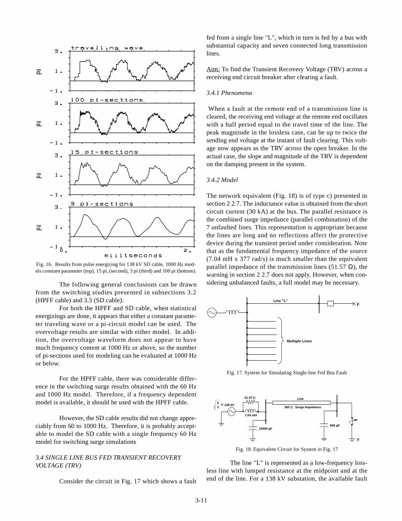
The results from the 1000 Hz models are shown inFig. 16. The limitations of the 3 and 15 section pi models areagain evident, although the 15 section model appears to givereasonably good results. Now, however, the constant param-eter and 100 section pi-circuit models give results that arevery close to each other. In the front edge of the first pulse, astair step effect can be seen. This is caused by voltagesinduced in the other two cables. Some oscillation can also beseen in these stair steps when the 100 section pi model isused. These oscillations are probably similar to the Gibb’sphenomenon encountered with Fourier Transforms.
3-11
Fig. 16. Results from pulse energizing for 138 kV SD cable, 1000 Hz mod-els constant parameter (top), 15 pi, (second), 3 pi (third) and 100 pi (bottom).
The following general conclusions can be drawnfrom the switching studies presented in subsections 3.2(HPFF cable) and 3.3 (SD cable):
For both the HPFF and SD cable, when statisticalenergizings are done, it appears that either a constant parame-ter traveling wave or a pi-circuit model can be used. Theovervoltage results are similar with either model. In addi-tion, the overvoltage waveform does not appear to havemuch frequency content at 1000 Hz or above, so the numberof pi-sections used for modeling can be evaluated at 1000 Hzor below.
For the HPFF cable, there was considerable differ-ence in the switching surge results obtained with the 60 Hzand 1000 Hz model. Therefore, if a frequency dependentmodel is available, it should be used with the HPFF cable.
However, the SD cable results did not change appre-ciably from 60 to 1000 Hz. Therefore, it is probably accept-able to model the SD cable with a single frequency 60 Hzmodel for switching surge simulations
3.4 SINGLE LINE BUS FED TRANSIENT RECOVERY VOLTAGE (TRV)
Consider the circuit in Fig. 17 which shows a fault
fed from a single line "L", which in turn is fed by a bus withsubstantial capacity and seven connected long transmissionlines.
Aim: To find the Transient Recovery Voltage (TRV) across areceiving end circuit breaker after clearing a fault.
3.4.1 Phenomena
When a fault at the remote end of a transmission line iscleared, the receiving end voltage at the remote end oscillateswith a half period equal to the travel time of the line. Thepeak magnitude in the lossless case, can be up to twice thesending end voltage at the instant of fault clearing. This volt-age now appears as the TRV across the open breaker. In theactual case, the slope and magnitude of the TRV is dependenton the damping present in the system.
3.4.2 Model
The network equivalent (Fig. 18) is of type c) presented insection 2 2.7. The inductance value is obtained from the shortcircuit current (30 kA) at the bus. The parallel resistance isthe combined surge impedance (parallel combination) of the7 unfaulted lines. This representation is appropriate becausethe lines are long and no reflections affect the protectivedevice during the transient period under consideration. Notethat as the fundamental frequency impedance of the source(7.04 mH x 377 rad/s) is much smaller than the equivalentparallel impedance of the transmission lines (51.57 Ω), thewarning in section 2 2.7 does not apply. However, when con-sidering unbalanced faults, a full model may be necessary.
Fig. 17. System for Simulating Single-line Fed Bus Fault
Fig. 18. Equivalent Circuit for System in Fig. 17
The line "L" is represented as a low-frequency loss-less line with lumped resistance at the midpoint and at theend of the line. For a 138 kV substation, the available fault
FLine "L"
Multiple Lines
Line
10000 pF
7.04 mH
600 pF
F
23
138 kV×51.57
360 Surge Impedance
Ω
Ω
3-12
current at the main bus is 30 kA and 3.7 kA at the fault loca-tion. Circuit parameters were selected for a 795 MCM line oflength 40 km to the fault location with a surge impedance of360 ohms.
Lumped bus capacitance of 10000 pF is representedat the supply station while 600 pF, which is typical for asmall substation, is represented at the station at the end of theline
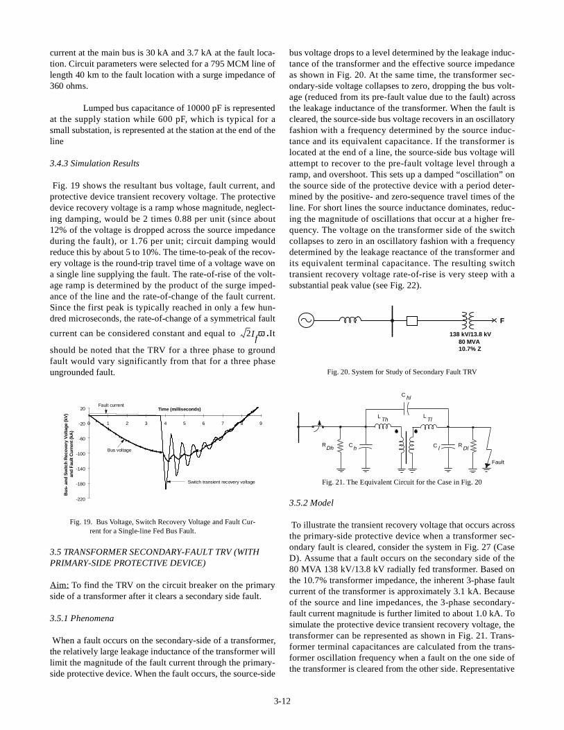
3.4.3 Simulation Results
Fig. 19 shows the resultant bus voltage, fault current, andprotective device transient recovery voltage. The protectivedevice recovery voltage is a ramp whose magnitude, neglect-ing damping, would be 2 times 0.88 per unit (since about12% of the voltage is dropped across the source impedanceduring the fault), or 1.76 per unit; circuit damping wouldreduce this by about 5 to 10%. The time-to-peak of the recov-ery voltage is the round-trip travel time of a voltage wave ona single line supplying the fault. The rate-of-rise of the volt-age ramp is determined by the product of the surge imped-ance of the line and the rate-of-change of the fault current.Since the first peak is typically reached in only a few hun-dred microseconds, the rate-of-change of a symmetrical fault
current can be considered constant and equal to .It
should be noted that the TRV for a three phase to groundfault would vary significantly from that for a three phaseungrounded fault.
Fig. 19. Bus Voltage, Switch Recovery Voltage and Fault Cur-rent for a Single-line Fed Bus Fault.
3.5 TRANSFORMER SECONDARY-FAULT TRV (WITH PRIMARY-SIDE PROTECTIVE DEVICE)
Aim: To find the TRV on the circuit breaker on the primaryside of a transformer after it clears a secondary side fault.
3.5.1 Phenomena
When a fault occurs on the secondary-side of a transformer,the relatively large leakage inductance of the transformer willlimit the magnitude of the fault current through the primary-side protective device. When the fault occurs, the source-side
bus voltage drops to a level determined by the leakage induc-tance of the transformer and the effective source impedanceas shown in Fig. 20. At the same time, the transformer sec-ondary-side voltage collapses to zero, dropping the bus volt-age (reduced from its pre-fault value due to the fault) acrossthe leakage inductance of the transformer. When the fault iscleared, the source-side bus voltage recovers in an oscillatoryfashion with a frequency determined by the source induc-tance and its equivalent capacitance. If the transformer islocated at the end of a line, the source-side bus voltage willattempt to recover to the pre-fault voltage level through aramp, and overshoot. This sets up a damped “oscillation” onthe source side of the protective device with a period deter-mined by the positive- and zero-sequence travel times of theline. For short lines the source inductance dominates, reduc-ing the magnitude of oscillations that occur at a higher fre-quency. The voltage on the transformer side of the switchcollapses to zero in an oscillatory fashion with a frequencydetermined by the leakage reactance of the transformer andits equivalent terminal capacitance. The resulting switchtransient recovery voltage rate-of-rise is very steep with asubstantial peak value (see Fig. 22).
Fig. 20. System for Study of Secondary Fault TRV
Fig. 21. The Equivalent Circuit for the Case in Fig. 20
3.5.2 Model
To illustrate the transient recovery voltage that occurs acrossthe primary-side protective device when a transformer sec-ondary fault is cleared, consider the system in Fig. 27 (CaseD). Assume that a fault occurs on the secondary side of the80 MVA 138 kV/13.8 kV radially fed transformer. Based onthe 10.7% transformer impedance, the inherent 3-phase faultcurrent of the transformer is approximately 3.1 kA. Becauseof the source and line impedances, the 3-phase secondary-fault current magnitude is further limited to about 1.0 kA. Tosimulate the protective device transient recovery voltage, thetransformer can be represented as shown in Fig. 21. Trans-former terminal capacitances are calculated from the trans-former oscillation frequency when a fault on the one side ofthe transformer is cleared from the other side. Representative
2I fω
Bus
- and
Sw
itch
Rec
over
y V
olta
ge (k
V)
and
Faul
t Cur
rent
(kA
)
-220
-180
-140
-100
-60
-20
20
0 1 2 3 4 5 6 7 8 9
Fault current
Bus voltage
Switch transient recovery voltage
T ime (milliseconds)
F
138 kV/13.8 kV80 MVA10.7% Z
Fault
RDh RDl
Chl
Ch C l
LThL
Tl

3-13
frequencies for power transformers are reported by Harnerand Rodriguez [24]. For the 138-kV winding, the frequencyof oscillation is approximately 9.6 kHz, while that of the13.8-kV winding is approximately 72.3 kHz. The high-fre-
quency capacitive coupling ratio (i.e., ) is
generally lower than 0.4 and was selected to be equal to 0.2for the simulation. As described in section 2.2.2, the capaci-tance is calculated from the known winding frequencies.
The effective terminal capacitances can be deter-mined based on the frequency of oscillation of each winding
by using the equation ,where f is the
frequency of oscillation of each of the windings in Hz, LT
(Henries) is the transformer leakage inductance (referred tothe winding of interest) and C (Farads) is the effective capac-itance. For the high-voltage winding:
and, for the low-voltage winding:
Based on the winding frequencies, and the trans-former leakage inductance of 67.48 mH (referred to the high-voltage winding), the winding terminal capacitances are:
Due to high-frequency winding resistance and eddycurrent losses, the oscillations are damped. This damping isrepresented by the resistance to ground in the equivalent cir-cuit shown in Fig. 21. For most transformers the damping isusually such that the damping factor (i.e., the ratio of succes-sive peaks of opposite polarity in the oscillation) is on theorder of 0.6 to 0.8. A conservative value of 0.8 was selectedfor this simulation. The time between peaks (of the same
polarity) of the oscillation is: , hence, for an
assumed damping factor, , the high-frequency damping
resistance, , can be calculated using the equation:
where L is the effective leakage inductance of the trans-former (referred to the winding of interest) and C is the effec-tive capacitance of the winding of interest.
Based on the transformer leakage inductance of67.48 mH and the terminal capacitances, the high-voltagewinding damping resistance is equal to 57.3 kΩ and that ofthe low-voltage winding is 7.48 kΩ.
3.5.3 Simulation Results
Fig. 22 shows the transient recovery voltage for the switch-ing device, the source-side and transformer-side voltages,and the 138 kV substation bus voltage for interrupting a faulton the secondary side of the transformer.
Fig. 22. Source, Transformer Side and 138 kV substation Bus Voltages for a Secondary Side Fault on a 80 MVA 138 kV/213.8 kV Transformer
3.6 SHUNT CAPACITOR SWITCHING
Aim: To present by example, modeling guidelines that shouldbe observed when simulating capacitor switching transients.A brief discussion of the transient phenomena associate withcapacitor switching is presented as background to the casestudy used to illustrate modeling guidelines. Understandingthe transient phenomena associated with any simulated eventwill allow a model of sufficient accuracy to be created whileavoiding needlessly complicated models that waste computerand engineering time.
3.6.1 Phenomena
Capacitor switching can cause significant transients at boththe switched capacitor and remote locations. The most com-mon transient problems when switching capacitors are (1)overvoltages at the switched capacitor during energization,(2) voltage magnification at lower voltage capacitors duringcapacitor energization, (3) transformer phase-to-phase over-voltages at a line termination during capacitor energization,(4) arrester energy duty during capacitor breaker restrike, (5)breaker current due to inrush from capacitors at the same busas a capacitor being energized and (6) breaker current due tooutrush from a capacitor into a nearby fault. Although all ofthese phenomena can be initiated by capacitor switching orfault initiation near a capacitor, they each produce differenttypes of transients that can adversely affect different powersystem apparatus. Some of the phenomena also have differ-ent modeling requirements. Each phenomena is briefly dis-cussed before being illustrating by example.
3.6.2 Switched Capacitor Overvoltages During Energization
Energizing a shunt capacitor from a predominately inductivesource results in an oscillatory transient voltage at the capac-itor bus with a magnitude that can approach twice the peakbus voltage prior to energization. The characteristic frequency
Chl Chl Cl+( )⁄
C 1 2πf( )2LT[ ]⁄=
C Ch Chl+=
C Cl Chl+=
Ch2.64nF=
Chl1.44nF=
Cl5.75nF=
1 f⁄ 2π LC=
DF
RD
RD
π LC----–
DFln---------------=
Per
uni
t pha
se-t
o-gr
ound
vol
tag
e
-2
-1.5
-1
-0.5
0
0.5
2.5 2.7 2.9 3.1 3.3 3.5 3.7 3.9
Time (milliseconds)
T rans former-s ide voltage
S ource-side voltage
Protective device transientrecovery voltage
138 kV S ubstation bus voltage

3-14
of the energization transient is:
where: LS = source inductance (Henries)C = capacitor bank capacitance (Farads)
This energization transient can excite system resonances orcause high frequency overvoltages at transformer termina-tions. The magnitude and duration of the energizing voltagetransient is dependent upon a number of factors including sys-tem strength, local transmission lines, system capacitances,and switching device characteristics. Voltage transient magni-tudes increase as system strength is reduced, relative to capac-itor size. In addition to reducing system surge impedance andincreasing system strength, transmission lines provide damp-ing. These three characteristics of transmission lines help re-duce capacitor energizing transients. Other capacitors in thevicinity of a switched bank help reduce capacitor energizingtransients because they reduce system surge impedance.Switching devices can be designed to reduce transients by us-ing closing control, pre-insertion resistors, or pre-insertion in-ductors. The closer to zero voltage at which a capacitor isenergized, the lower the resulting transients. The optimumclosing resistor size is approximately equal to the surge imped-ance of the source inductance and capacitor bank capacitanceas calculated below:
where: LS = source inductance (H)C = capacitor bank capacitance (F)
3.6.3 Voltage Magnification at Lower Voltage Capacitors
Normal capacitor bank energizing transients, which are limitedto twice the pre-switch capacitor bus voltage, are not a concernat the switched capacitor location. Significant transient voltag-es can occur at remote capacitors or cables when magnificationof the capacitor energizing transient occurs. The simple circuitin Fig. 23 illustrates the voltage magnification phenomena.
Fig. 23. Circuit Illustrating Voltage Magnification
The highest transient voltages, on a per unit basis, occur at thelower voltage capacitance (C2) during capacitor C1 energiza-
tion when (1) the capacitive Mvar rating of C1 is significantly
greater than that of C2 and (2) the natural frequencies f1 and f2(as defined below) are nearly equal.
and
The magnitude of the voltage magnification transient at C2 isdependent on switched capacitor size, source impedance, theimpedance between the two capacitances, system loading, andthe existence of other nearby low voltage capacitors. Moderateincreases in distribution system loading can significantly re-duce voltage magnification transients. Because transformerlosses increase significantly at higher frequencies, modelingthe frequency dependence of transformer losses, or simplymodeling the transformer X/R ratio at the capacitor’s naturalfrequency, can improve model accuracy and reduce the sever-ity of the voltage magnification simulated. Controlled breakerclosing, pre-insertion resistors, or pre-insertion inductors canbe used to reduce voltage magnification related transients.
Voltage magnification can also cause excessiveenergy duty at arresters protecting distribution capacitors.High energy arresters may be necessary if other methods ofreducing voltage magnification are not implemented.
3.6.4 Transformer Termination Phase-to-Phase Overvoltages
Capacitor energization can initiate traveling waves that will in-crease in magnitude when reflected at transformer termina-tions. These reflected surges will be limited to approximatelytwo per unit by the transformer line-to-ground arresters. Fourper unit phase-to-phase voltage transients can be caused by 2pu surges of opposite polarity appearing simultaneously ondifferent phases. This four per unit switching transient may ex-ceed a transformer’s switching surge withstand capability.IEEE standards do not specify transformer phase-to-phaseswitching surge withstand capability. As a worst case assump-tion, the phase-to-ground withstand could be used, but a valuecloser to 3.4 pu is probably more realistic. The transformermanufacturer should be consulted to determine the phase-to-phase switching surge withstand voltage of a specific trans-former.
System short circuit capability and the number of lines at theswitched capacitor location do not significantly affect this phe-nomena. Switched capacitor size affects the frequency of os-cillation that occurs when a capacitor is energized, and thus thevoltage that the traveling wave component of the transientrides on, but no generalization relating capacitor bank size andreflected phase-to-phase transient can be made. Radial linelength may have a more predicable effect. Higher phase-to-phase transients often occur on longer lines as the travelingwave oscillation peak begins to match up with the natural fre-quency of the capacitor energization transient. Oscillationsthat occur on very short lines may also be important, as theyhave the potential for exciting transformer internal resonances.
f1
2π LSC------------------=
Roptimum
LSC------=
f11
2π L1C1
--------------------= f21
2π L2C2
--------------------=
3-15
As with other capacitor switching related transients, thesetransients can be reduced by the use of synchronous closingcontrol, pre-insertion resistors, or pre-insertion inductors.
3.6.5 Capacitor Breaker Restrike Arrester Energy Duty
Arresters applied at large shunt capacitors should be evaluat-ed for their energy duty during capacitor breaker restrike. Thisis true even when the capacitor breakers are designed to be“restrike free.”
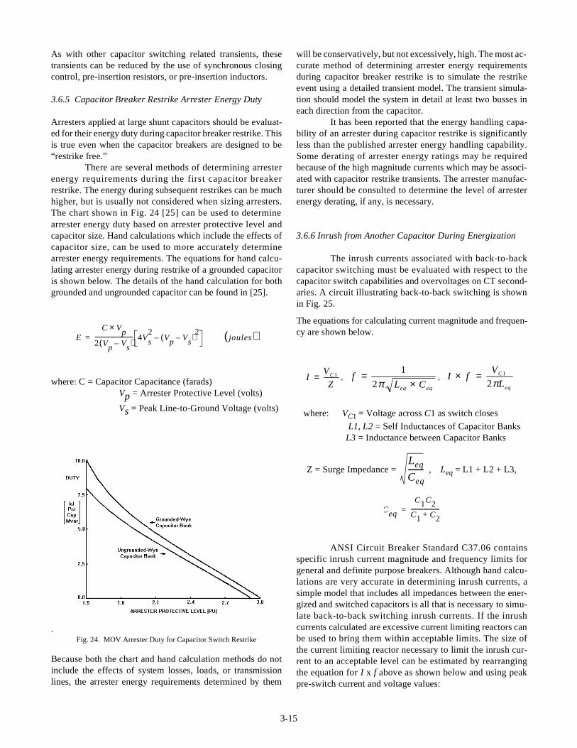
There are several methods of determining arresterenergy requirements during the first capacitor breakerrestrike. The energy during subsequent restrikes can be muchhigher, but is usually not considered when sizing arresters.The chart shown in Fig. 24 [25] can be used to determinearrester energy duty based on arrester protective level andcapacitor size. Hand calculations which include the effects ofcapacitor size, can be used to more accurately determinearrester energy requirements. The equations for hand calcu-lating arrester energy during restrike of a grounded capacitoris shown below. The details of the hand calculation for bothgrounded and ungrounded capacitor can be found in [25].
where: C = Capacitor Capacitance (farads)Vp = Arrester Protective Level (volts)
Vs = Peak Line-to-Ground Voltage (volts)
.Fig. 24. MOV Arrester Duty for Capacitor Switch Restrike
Because both the chart and hand calculation methods do notinclude the effects of system losses, loads, or transmissionlines, the arrester energy requirements determined by them
will be conservatively, but not excessively, high. The most ac-curate method of determining arrester energy requirementsduring capacitor breaker restrike is to simulate the restrikeevent using a detailed transient model. The transient simula-tion should model the system in detail at least two busses ineach direction from the capacitor.
It has been reported that the energy handling capa-bility of an arrester during capacitor restrike is significantlyless than the published arrester energy handling capability.Some derating of arrester energy ratings may be requiredbecause of the high magnitude currents which may be associ-ated with capacitor restrike transients. The arrester manufac-turer should be consulted to determine the level of arresterenergy derating, if any, is necessary.
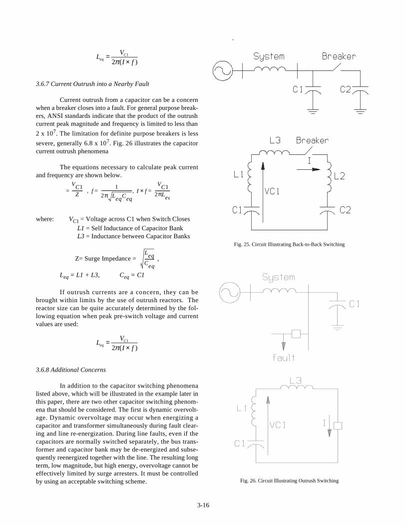
3.6.6 Inrush from Another Capacitor During Energization
The inrush currents associated with back-to-backcapacitor switching must be evaluated with respect to thecapacitor switch capabilities and overvoltages on CT second-aries. A circuit illustrating back-to-back switching is shownin Fig. 25.
The equations for calculating current magnitude and frequen-cy are shown below.
where: VC1 = Voltage across C1 as switch closes
L1, L2 = Self Inductances of Capacitor Banks L3 = Inductance between Capacitor Banks
Z = Surge Impedance = , Leq = L1 + L2 + L3,
ANSI Circuit Breaker Standard C37.06 contains
specific inrush current magnitude and frequency limits forgeneral and definite purpose breakers. Although hand calcu-lations are very accurate in determining inrush currents, asimple model that includes all impedances between the ener-gized and switched capacitors is all that is necessary to simu-late back-to-back switching inrush currents. If the inrushcurrents calculated are excessive current limiting reactors canbe used to bring them within acceptable limits. The size ofthe current limiting reactor necessary to limit the inrush cur-rent to an acceptable level can be estimated by rearrangingthe equation for I x f above as shown below and using peakpre-switch current and voltage values:
EC Vp×
2 Vp Vs–( )--------------------------- 4Vs
2Vp Vs–( )
2–= joules( )
IV
ZC= 1 , f
L Ceq eq
=×
1
2π, I f
V
LC
eq
× = 1
2π
Leq
Ceq--------
Ceq
C1C2C1 C2+--------------------=
3-16
3.6.7 Current Outrush into a Nearby Fault
Current outrush from a capacitor can be a concernwhen a breaker closes into a fault. For general purpose break-ers, ANSI standards indicate that the product of the outrushcurrent peak magnitude and frequency is limited to less than
2 x 10⁷. The limitation for definite purpose breakers is less
severe, generally 6.8 x 10⁷. Fig. 26 illustrates the capacitorcurrent outrush phenomena
The equations necessary to calculate peak currentand frequency are shown below.
where: VC1 = Voltage across C1 when Switch Closes
L1 = Self Inductance of Capacitor Bank L3 = Inductance between Capacitor Banks
Z= Surge Impedance = ,
Leq = L1 + L3, Ceq = C1
If outrush currents are a concern, they can bebrought within limits by the use of outrush reactors. Thereactor size can be quite accurately determined by the fol-lowing equation when peak pre-switch voltage and currentvalues are used:
3.6.8 Additional Concerns
In addition to the capacitor switching phenomenalisted above, which will be illustrated in the example later inthis paper, there are two other capacitor switching phenom-ena that should be considered. The first is dynamic overvolt-age. Dynamic overvoltage may occur when energizing acapacitor and transformer simultaneously during fault clear-ing and line re-energization. During line faults, even if thecapacitors are normally switched separately, the bus trans-former and capacitor bank may be de-energized and subse-quently reenergized together with the line. The resulting longterm, low magnitude, but high energy, overvoltage cannot beeffectively limited by surge arresters. It must be controlledby using an acceptable switching scheme.
.
Fig. 25. Circuit Illustrating Back-to-Back Switching
Fig. 26. Circuit Illustrating Outrush Switching
)(21
fI
VL C
eq ×=
π
IVC1
Z-----------= f,
1
2π LeqCeq
------------------------------- I f×,VC1
2πLeq----------------= =
LeqCeq----------
)(21
fI
VL C
eq ×=
π
3-17
Another concern when switching shunt capacitor banks is in-ternal overvoltages at remote transformers. These overvoltag-es are a function of the switching transient and transformerinternal resonance characteristics. Transformer terminal ar-resters may not adequately protect for this condition. Possiblesolutions include (1) capacitor switch pre-insertion resistorsor reactors and (2) capacitor bank reactors.
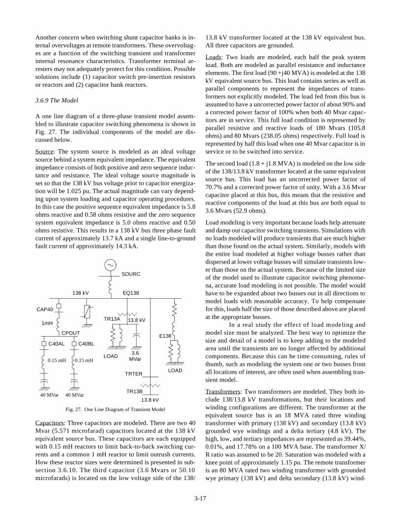
3.6.9 The Model
A one line diagram of a three-phase transient model assem-bled to illustrate capacitor switching phenomena is shown inFig. 27. The individual components of the model are dis-cussed below.
Source: The system source is modeled as an ideal voltagesource behind a system equivalent impedance. The equivalentimpedance consists of both positive and zero sequence induc-tance and resistance. The ideal voltage source magnitude isset so that the 138 kV bus voltage prior to capacitor energiza-tion will be 1.025 pu. The actual magnitude can vary depend-ing upon system loading and capacitor operating procedures.In this case the positive sequence equivalent impedance is 5.8ohms reactive and 0.58 ohms resistive and the zero sequencesystem equivalent impedance is 5.0 ohms reactive and 0.50ohms resistive. This results in a 138 kV bus three phase faultcurrent of approximately 13.7 kA and a single line-to-groundfault current of approximately 14.3 kA.
Fig. 27. One Line Diagram of Transient Model
Capacitors: Three capacitors are modeled. There are two 40Mvar (5.571 microfarad) capacitors located at the 138 kVequivalent source bus. These capacitors are each equippedwith 0.15 mH reactors to limit back-to-back switching cur-rents and a common 1 mH reactor to limit outrush currents.How these reactor sizes were determined is presented in sub-section 3.6.10. The third capacitor (3.6 Mvars or 50.10microfarads) is located on the low voltage side of the 138/
13.8 kV transformer located at the 138 kV equivalent bus.All three capacitors are grounded.
Loads: Two loads are modeled, each half the peak systemload. Both are modeled as parallel resistance and inductanceelements. The first load (90 +j40 MVA) is modeled at the 138kV equivalent source bus. This load contains series as well asparallel components to represent the impedances of trans-formers not explicitly modeled. The load fed from this bus isassumed to have a uncorrected power factor of about 90% anda corrected power factor of 100% when both 40 Mvar capac-itors are in service. This full load condition is represented byparallel resistive and reactive loads of 180 Mvars (105.8ohms) and 80 Mvars (238.05 ohms) respectively. Full load isrepresented by half this load when one 40 Mvar capacitor is inservice or to be switched into service.
The second load (1.8 + j1.8 MVA) is modeled on the low sideof the 138/13.8 kV transformer located at the same equivalentsource bus. This load has an uncorrected power factor of70.7% and a corrected power factor of unity. With a 3.6 Mvarcapacitor placed at this bus, this means that the resistive andreactive components of the load at this bus are both equal to3.6 Mvars (52.9 ohms).
Load modeling is very important because loads help attenuateand damp out capacitor switching transients. Simulations withno loads modeled will produce transients that are much higherthan those found on the actual system. Similarly, models withthe entire load modeled at higher voltage busses rather thandispersed at lower voltage busses will simulate transients low-er than those on the actual system. Because of the limited sizeof the model used to illustrate capacitor switching phenome-na, accurate load modeling is not possible. The model wouldhave to be expanded about two busses out in all directions tomodel loads with reasonable accuracy. To help compensatefor this, loads half the size of those described above are placedat the appropriate busses.
In a real study the effect of load modeling andmodel size must be analyzed. The best way to optimize thesize and detail of a model is to keep adding to the modeledarea until the transients are no longer affected by additionalcomponents. Because this can be time consuming, rules ofthumb, such as modeling the system one or two busses fromall locations of interest, are often used when assembling tran-sient model.
Transformers: Two transformers are modeled. They both in-clude 138/13.8 kV transformations, but their locations andwinding configurations are different. The transformer at theequivalent source bus is an 18 MVA rated three windingtransformer with primary (138 kV) and secondary (13.8 kV)grounded wye windings and a delta tertiary (4.8 kV). Thehigh, low, and tertiary impedances are represented as 39.44%,0.01%, and 17.78% on a 100 MVA base. The transformer X/R ratio was assumed to be 20. Saturation was modeled with aknee point of approximately 1.15 pu. The remote transformeris an 80 MVA rated two winding transformer with groundedwye primary (138 kV) and delta secondary (13.8 kV) wind-
SOURC
138 kV
CAP40
1mH
C40AL C40BL
TR13A
LOAD3.6
MVar
13.8 kV
LOAD
E138CPOUT
13.8 kV
TR13B
TRTER
EQ138
0.15 mH 0.15 mH
40 MVar 40 MVar
3-18
ings. The transformer impedances is 10.7% on its 80 MVAbase. Half this impedance is modeled on each winding. Thetransformer X/R ratio was assumed to be 20. Saturation wasmodeled with an approximately 1.2 pu knee.
Line Model: The line modeled is a 40 km long 138 kV lineconnecting the equivalent source bus with the remote buslabeled “TRTER”. The line uses 477 ACSR “Hawk” conduc-tor in a horizontal configuration. The conductor has 27 alu-minum strands and 6 steel strands, a DC resistance of 0.1221ohms per km at 25 degrees C, and a geometric mean radius of0.884 cm. Because of the need to accurately model voltagereflections at transformer terminated lines, this line was mod-eled using a frequency dependent distributed parametertransmission line model.
Surge Arrester Model: Following normal practices on solidlygrounded 138 kV systems, a 108 kV station class gaplessMOV surge arrester was included at the capacitor location.The non-linear arrester characteristic is modeled by a numberof exponential segments based on the arrester’s 36/90 µseccurrent/voltage characteristics. Arrester energy was moni-tored during capacitor breaker restrike. Fault Model: The fault model used in the outrush simula-tions is a 0.1 milliohm resistance in series with an idealswitch. When the fault is initiated, the switch is closed andwhen the fault is cleared the switch is opened.
3.6.10 Simulation Results:
Simulations were run to illustrate four different capacitorswitching events: capacitor energizing, capacitor breaker re-strike during de-energization, back-to-back capacitor inrush,and capacitor outrush into a fault. Each of these events are dis-cussed below.
Capacitor Energization: Capacitor energization was simu-lated to demonstrate three different phenomena. The first isthe transient overvoltage at the switched capacitor location.The second is voltage magnification at a lower voltagecapacitor. The third is phase-to-phase overvoltage at a trans-former terminated line.
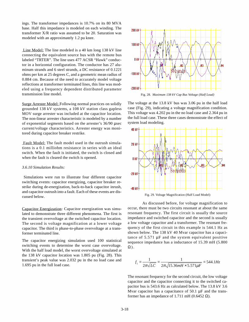
The capacitor energizing simulation used 100 statisticalswitching events to determine the worst case overvoltage.With the half load model, the worst overvoltage simulated atthe 138 kV capacitor location was 1.805 pu (Fig. 28). Thistransient’s peak value was 2.032 pu in the no load case and1.695 pu in the full load case.
Fig. 28. Maximum 138 kV Cap Bus Voltage (Half Load)
The voltage at the 13.8 kV bus was 3.06 pu in the half loadcase (Fig. 29), indicating a voltage magnification condition.This voltage was 4.202 pu in the no load case and 2.364 pu inthe full load case. These three cases demonstrate the effect ofsystem load modeling.
Fig. 29. Voltage Magnification (Half Load Model)
As discussed before, for voltage magnification tooccur, there must be two circuits resonant at about the sameresonant frequency. The first circuit is usually the sourceimpedance and switched capacitor and the second is usuallya low voltage capacitor and a transformer. The resonant fre-quency of the first circuit in this example is 544.1 Hz asshown below. The 138 kV 40 Mvar capacitor has a capaci-tance of 5.571 µF and the system equivalent positivesequence impedance has a inductance of 15.39 mH (5.800Ω ) .
The resonant frequency for the second circuit, the low voltagecapacitor and the capacitor connecting it to the switched ca-pacitor bus is 543.6 Hz as calculated below. The 13.8 kV 3.6Mvar capacitor has a capacitance of 50.1 µF and the trans-former has an impedance of 1.711 mH (0.6452 Ω).
HzFmHLC
f 1.544571.536.152
1
2
11 =
×==
µππ

3-19
Voltage magnification results from the fact that the two reso-nance frequencies are so close together.
The third phenomena of concern during capacitor energiza-tion is excessive phase-to-phase voltages at the end of a trans-former terminated line. As previously discussed, if this valueexceeds 3.4 pu there should be some concern for the trans-former insulation. In the half load case, the maximum phase-to-phase voltage simulated at the remote transformer’s 138kV terminals was 4.895 pu (Fig. 30). Phase-to-phase overvolt-ages of 5.286 and 4.673 were simulated under no load and fullload conditions. All of these voltages were simulated withoutarresters modeled. If arresters were modeled at the transform-er terminals, the phase to phase overvoltage would be limitedto twice the arrester discharge voltage, approximately 4 pu.
Breaker Restrike: The most severe energy duty for arrestersapplied at capacitor bank locations is often when a breaker re-strikes as a capacitor is taken out of service. For capacitorswitching transients, an arrester’s kJ/kV rating may be have tobe derated. The arrester manufacturer should be consulted todetermine the derating for a specific arrester. Since a properlyfunctioning breaker will always open at a current zero, statis-tical simulations are not required when simulating capacitorrestrike. Generally only one phase of a breaker will restrikeand, while the phase may reopen soon after the restrike, re-strikes are often simulated as being permanent. Restrike ismost severe when it occurs at the time of peak breaker tran-sient recovery voltage (TRV). The breaker TRVs simulatedwhen a restrike occurs as both 40 Mvar capacitors in the halfload model are opened is shown in Fig. 31.
Fig. 30. Ph-to-Ph Voltage at Remote Transformer (Half Load)
Fig. 31. Restrike Breaker TRV (Half Load Model)
The 108 kV Station Class arrester modeled has a switchingsurge protective level of 200 kV line-to-ground, 1.775 pu onthe 138 kV system. According to Figure 2, this arrester wouldhave to be able to dissipate about 6 kJ/kV of arrester rating.This may be excessive after derating the normal 7.2 kJ/kV ofrated voltage (8.9 kJ/kV of MCOV) of a station class arresterenergy used for capacitor protection. Under this conditiontransient simulation is necessary.
Simulated arrester voltages during capacitor breaker restrikeare shown in Fig. 32.
The simulated energy duty of the capacitor arrester,263 kJ, is shown in Fig. 33. A 108 kV station class arrestercan be expected to be able to dissipate about 778 kJ undernormal conditions. Derating the arrester energy handingcapability by half for capacitor breaker restrike still gives 389kJ of capability, well above the 263 kJ required. Althoughnot examined in this case, arrester energies at remote capaci-tors where voltage magnification may occurred should alsobe monitored.
Fig. 32. Arrester Bus Voltages During Capacitor Breaker Restrike
HzFmHLC
f 6.5431.50711.12
1
2
12 =
×==
µππ

3-20
Fig. 33. Arrester Energy During Breaker Restrike
Capacitor Inrush During Back-to-Back Switching: The con-cern during back-to-back switching is that capacitor inrushcurrents will exceed breaker ratings. The magnitude and fre-quency of the inrush current can exceed breaker capabilitiesif the impedance between the two capacitors is too low.Breakers applied between two capacitor banks at a single busare usually definite purpose breakers. According to Table 3Aof ANSI/IEEE C37.06, the product of the breaker current
magnitude and frequency must be less than 6.8 x 10⁷ (16 kAtimes 4250 Hz) for definite purpose breakers.
An equation for calculating the inductance necessary to limitthe I x f product to an acceptable level was given in subsection3.6.6. With Vmax equal to the peak line-to-ground voltage,times a conservative 1.05 pu voltage, the inductance neces-
sary to meet the 6.8 x 10⁷ breaker rating can be calculated tobe 0.277 mH or 0.139 mH per capacitor as shown below.Some of this inductance may be supplied by the buswork be-tween the two capacitors. Buswork rated for use on 138 kVsystems is usually considered to have an inductance of 0.9 µHper meter.
Back-to-back capacitor switching inrush currents are inde-pendent of load or nearby system components. Inrush currentswere simulated with a with a 0.15 mH reactor in series witheach 40 Mvar 138 kV capacitor. This resulted in a peak cur-rent of 12 kA at a frequency of 5.5 kHz, giving an I x f product
of 6.6 x 10⁷, below the 6.8 x 10⁷ limit.
Capacitor Outrush into a Fault: The concern during capaci-tor outrush into a fault is again breaker I x f ratings, butbecause the fault current may go through a general purposebreaker rather than a definite purpose breaker, the breaker I x
f rating will probably be a much lower 2.0 x 10⁷ rather than
6.8 x 10⁷. The equation derived in subsection 3.6.7 can beused, but the I x f product will be different and the reactormust placed so that the fault current discharged from bothcapacitors will have to flow through the reactor to get to themain bus, as shown between busses CAP40 and CPOUT in
Figure 5. In this case the reactor size was calculated to be0.942 mH, as shown below.
An outrush reactor value of 1.0 mH was used to simulate thisevent. This simulation gave a peak current (first current peak)of 1,966 amps at a frequency of 9,454 Hz. This results in an I
x f product of 1.86 x 10⁷, which is below the 2.0 x 10⁷ limit.
3.7 SERIES CAPACITOR SWITCHING
Series capacitors may be installed on transmissionlines to increase power transfer capability. Electromagnetictransient studies are required to determine the impact of theseries compensation on the existing system to ensure safeand reliable operation.Aim: To evaluate several aspects of system performance,including the following:• Surge Arrester Sizing: Establish surge arrester duty and
related protection settings for the capacitor bank.• Line Protection: Investigate relay requirements.• Line Breaker Transient Recovery Voltage (TRV): Deter-
mine the transient recovery voltage for the transmission line breakers of the compensated line.
• Line Energization: Investigate system behavior when the compensated line is energized.
• Bank Insertion and Bypass: Investigate system behavior when the series capacitor is bypassed or inserted.
• Single-Phase Reclosing: Determine line end arrester duty for single-phase reclosing operation.
Simulated events include varying size and locationof the series capacitor. However, these are generally deter-mined by steady-state, transient stability and subsynchronousresonance studies and by relaying requirements which arenot applicable to this document. Additionally, minimum andmaximum generator conditions may also be considered.
3.7.1 Model
Fig. 34 shows a representative system to be studied.The system model typically includes lines and transformersat least one bus back from the switching locations of interest.Transmission lines are modeled as distributed parameterlines considering their positive and zero sequence character-istics. Transformers are modeled using the saturable trans-former component model which represents each winding ofthe transformer as well as its saturation characteristics. Onebus away are equivalent sources modeled as mutually-cou-pled elements considering their positive and zero sequencecharacteristics. Series capacitors and other system compo-nents are modeled as lumped circuit elements with typicalquality factors represented. Also pertaining to series capaci-
mHkV
fI
VL 277.0
)108.6(2
31.118
)(2 7max =
×=
×=
ππ
mHkV
fI
VL 942.0
)102(2
31.118
)(2 7max =
×=
×=
ππ

3-21
tor modeling are its associated components such as thebypass breaker with its series reactor and the surge arresterconnected across the series capacitor. The surge arrestermodel uses the 36x90 µs voltage-current characteristic.
3.7.2 Phenomena and Simulation Results
The worst case fault conditions that keep the capac-itor bank inserted determine the maximum surge arresterenergy requirements. The case list includes three-phase, dou-ble-phase and single-phase faults. Also considered are sin-gle-phase reclosing events under fault conditions: the lineend breakers open on the faulted phase only to clear the fault,and then one end recloses.
Line protection may be evaluated by monitoringcurrents that would flow in the line relays during three-phaseand single-phase faults which are internal or external to thecapacitor bank.
The maximum TRV of line breakers may be evalu-ated by applying three-phase and single-phase faults at vari-ous locations along the line and at the series capacitor. Insome cases arresters or pre-insertion devices may be requiredto reduce the TRV to acceptable levels.
The effect of energizing the series compensated linewith and without the capacitor bypassed can be evaluated.
The impact of capacitor bank insertion and bypass
should be simulated under varying power flow and otheroperating conditions. The bypass switch TRV is evaluatedfrom the simulation of capacitor bank insertion. The simula-tion of capacitor bypass determines the inrush currents.Results are compared to the withstand ratings at the breakerand its series reactor.
Waveforms of sample results are shown 5 for theseswitching transients cases:
i ) Single-Phase Fault, Clearing, and Reclosing (Fig. 35)ii ) Three-Phase Fault at Middle of Line and Clearing (Fig.
36 and Fig. 37)iii ) Series Capacitor Bank Insertion (Fig. 38)
4. CONCLUSIONS
This report presented general rules for the study ofswitching surges using electromagnetic transients simulation.The main goal is to have as simple a model as possible with-out a significant loss in accuracy. In addition to the modelingrepresentations, general concerns such as the time-step to beused and the extent of the system to be studied were alsoaddressed. The modeling techniques were illustrated withcase studies on line energization, TRV, shunt capacitor bankswitchings and series capacitor bank switchings.
Fig. 34. System Model for Series Capacitor Study
BUS 1115 KV
BUS 2115 KV
69 KV
69 KV

3-22
Fig. 35. Simulation Results: Single-Phase Fault, Clearing, and Reclosing
Fig. 36. Simulation Results: Three-Phase Fault at Middle of Line and Clearing
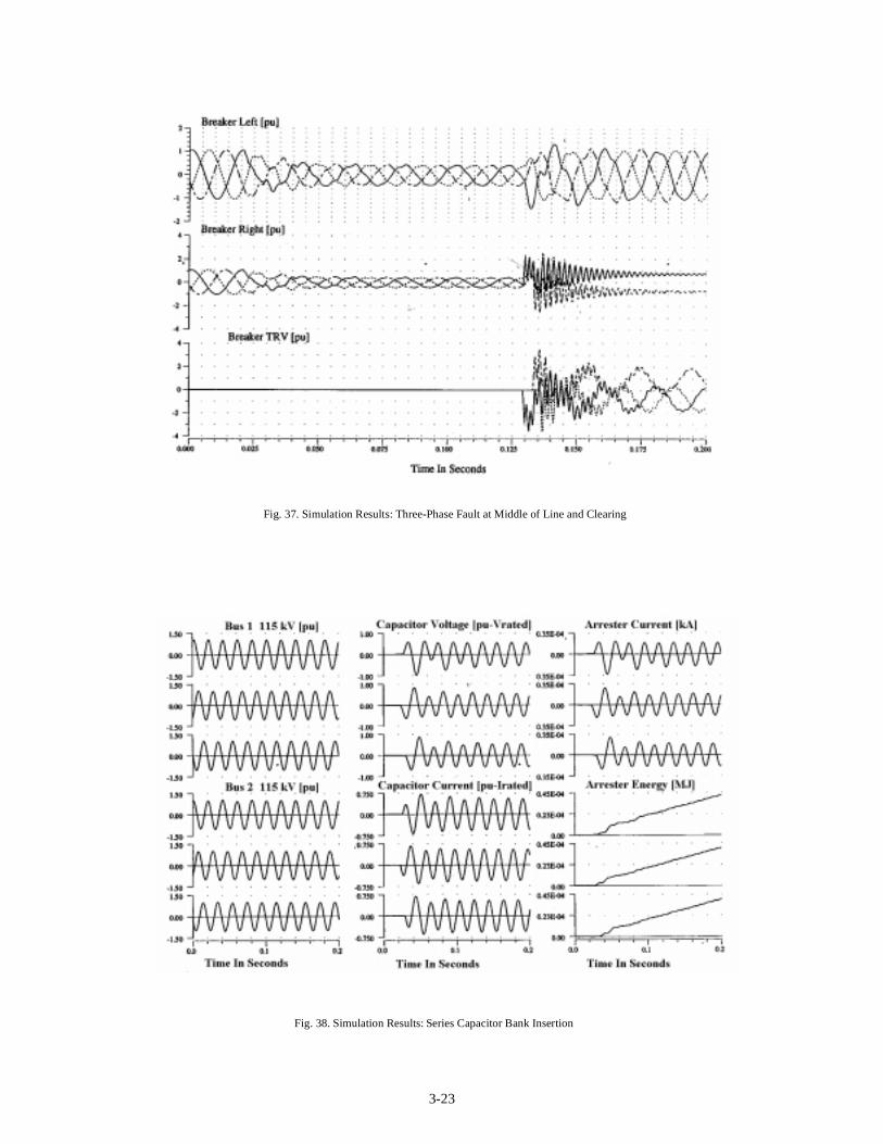
3-23
Fig. 37. Simulation Results: Three-Phase Fault at Middle of Line and Clearing
Fig. 38. Simulation Results: Series Capacitor Bank Insertion

3-24
V. REFERENCES
[1] H. W. Dommel, “Electromagnetic Transients Program Reference Manual (EMTP Theory Book)”, Report Pre-pared for Bonneville Power Administration, Portland, Oregon, August 1986.
[2] Moore, R.K, “Travelling-Wave Engineering, McGraw Hill, New York, 1960
[3] H.W. Dommel and J.R. Marti, “Overhead Line Parame-ters from Handbook Formulas and Computer Pro-grams”, IEEE Trans. PAS, Vol. PAS-104, No. 2, February 1985, pp. 366-372.
[4] C. J. Truax, J.D. Brown, and W. Neugebauer, “The Study of Reclosing Transients on a 765 kV Shunt Com-pensated Transmission Line”, IEEE Trans. PAS, Vol. PAS-97, No.4, July/August 1978, pp.1447-1457.
[5] “Guidelines for Representation of Network Elements when Calculating Transients”, CIGRE Subcommittee 33, Working Group 02 Report, 1990.
[6] V. Brandwajn, H.W. Dommel and I.I. Dommel, “Matrix Representation of Three Phase N-Winding Transformers for Steady State and Transient Studies”, IEEE Trans. PAS, Vol PAS-101, No.6, June 1982, pp. 1369-1378.
[7] R.C. Degeneff, "A Method for Constructing Terminal Models for Single Phase N- Winding Transformers", IEEE PES Summer Power Meeting, Los Angeles, July 1978, Paper A78 539-9.
[8] A. Morched, L. Marti, and J. Ottevangers, “A High Fre-quency Transformer Model for the EMTP”, IEEE Trans. PWRD, Vol. 8, No. 3, July 1993, pp. 1615-1626.
[9] R.J. Galarza, J.H. Chow and R.C. Degeneff, "Trans-former Model Reduction using Time and Frequency Domain Sensitivity Techniques”, IEEE Trans. PWRD, Vol. 10, No. 2, April 1995, pp. 1052-1058.
[10] F. De Leon and A. Semlyen, “Reduced Order Model for Transformer Transients”, IEEE Trans. PWRD, Vol. 7, No. 1, January 1992, pp. 376-383.
[11] W.J. McNutt, T.J. Blalock and R.A. Hinton, “Response of Transformer Windings to System Voltages”, IEEE Trans. PAS, Vol. PAS-93, No. 2, March/April 1974, pp. 457-467.
[12] V. Vanderstockt, "Use of Statistical and Systematic Switches", EMTP News, Vol.3, No.4, December 1990, pp. 12-30.
[13] D.A. Woodford and L.M. Wedepohl, “Transmission Line Energization with Breaker Pre-Strike”, IEEE WES-CANEX Conference on Communications, Power and Computing, Winnipeg, Canada, May 22-23, 1997, Pro-ceedings: pp. 105-108.(IEEE Catalog No. 97CH36117).
[14] CIGRE Working Group 13-02, “Interruption of Small Inductive Currents, Chapters 1 & 2”, ELECTRA, No. 72, 1980, pp. 73-102.
[15] CIGRE Working Group 13-02, “Interruption of Small Inductive Currents, Chapter 4: Reactor Switching, Part A”, ELECTRA, No. 101, 1985, pp. 51-74.
[16] J.A. Martinez-Velasco, “Circuit Breaker Representation for TRV Calculation”, EMTP/ATP Users’ Group Meet-ing, Hannover, November 13-15. 1995.
[17] J. Sousa, D. Santos and M.T. Correira de Barros, “Fault Arc Modeling in EMTP”, International Conference on Power Systems Transients, Lisbon, September 3-7, 1995, Proceedings, pp. 475-480.
[18] S. Goldberg, W.F. Horton and D. Tziouvaras, “A com-puter Model of the Secondary Arc in Single-phase Oper-ation of Transmission Lines”, IEEE Trans. PWRD, Vol. 4, No. 1, January 1989, pp. 586-595.
[19] D. W. Durbak, “The Choice of EMTP Surge Arrestor Models”, EMTP Newsletter, Vol. 7, No. 3, September 1987, pp. 14-18.
[20] A.S. Morched and V. Brandwajn, “Transmission Net-work Equivalents for Electromagnetic Transients Stud-ies”, IEEE Trans. PAS, Vol. PAS-102, No. 9, September 1983, pp. 2984-2994.
[21] A.S. Morched, J.H. Ottevangers and L. Marti, “Multi-port Frequency Dependent Network Equivalents for the EMTP”, IEEE Trans. PWRD, Vol. 8, No. 3, July 1993, pp. 1402-1412.
[22] A.M. Gole, I.T. Fernando, G.D. Irwin and O.B. Nayak, “Modeling of Power Electronic Apparatus: Additional Interpolation Issues”, International Conference on Power System Transients, Seattle, June 1997, Proceed-ings, pp. 23-28.
[23] CIGRE WG 13.02, “Switching Overvoltages in EHV and UHV Systems with Special Reference to Closing and Reclosing of Transmission Lines”, ELECTRA, No. 30, October 1973, pp. 70-122.
[24] R.H. Harner and J. Rodriguez, “Transient Recovery Voltages Associated with Power-System Three-Phase Transformer Secondary Faults”, IEEE Trans. PAS, Vol. PAS-91, No. 5, September/October 1972, pp.1887-1896.
[25] W.E. Reid, M. F. McGranaghan, S. W. Law and D.W. Gresham, “Overvoltage Protection of Shunt Capacitor Banks Using MOV Arresters”, IEEE Trans. PAS, Vol. PAS-103, No. 8, August 1984, pp. 2326-2333.