Modeling full scale-data(2)

Process Optimization: Enhancing

Understanding through Mining Full-

Scale Data

John B. Cook, PE, M.ASCE

Edwin A. Roehl

Uwe Mundry

Advanced Data Mining Int’l

Greenville, SC

Acknowledgement

Ed Roehl – CTO• World class industrial researcher;

• Software design, development, and project management;

• Advanced process engineering, computer-based modeling and optimization methods, industrial R&D, product/process design automation, CAE, PDM;

• Data mining, multivariate analysis, predictive modeling, simulation, advanced control, signal processing, non-linear/chaotic systems, computational geometry;

• AI, expert systems, OOP/computer languages, machine learning/artificial neural networks.

Uwe Mundry, Partner• World class software design, development;

• multi--spectral and hyper-spectral imaging and pattern recognition, 4D medical imaging, 4D geographical imaging, homeland security applications, real-time decision support systems with industrial applications; Data mining, multivariate analysis, predictive modeling, simulation, advanced control, signal processing, non-linear/chaotic systems, computational geometry, machine learning/artificial neural networks; OOP/multiple computer languages; Medical and environmental imaging.

Why optimize your plant?

• Reduced operating budgets (10% very

common)

• Increasingly stringent regulations

--Water treatment?

--Wastewater treatment?

• Increasing cost of capital improvements

--USD worth less

--QE2 will lower value of debt instruments such

as bonds

Process optimization by modeling

1. Modeling processes through various

means

a. Bench-scale models

b. Pilot-scale models

c. Mathematical models

1) Deterministic/mechanistic—based on first principles

2) Empirical—either statistical or based upon some

optimal function to describe behavior

3) Hybrid of 1) and 2)

Process optimization by modeling

What is a mathematical model?

―…..consistent set of mathematical equations which

is thought to correspond to some other entity, its

prototype.‖—Rutherford Aris

Definitions for pilot-scale modeling

• Geometric Similarity—All lengths of the model and the

prototype must be in the same ratio. All corresponding

angles must be equal. [This is the easy one to achieve.]

• Kinematic Similarity—Ratios of fluid velocity and other

relevant velocities must be the same for the model and

prototype. Ratios of flow time scale and boundary time

scale must be the same. [Problems with laminar/turbulent.]

• Dynamic Similarity—The force polygons for the model

and prototype must be proportional. For example, forces

such as inertia, pressure, viscous forces, surface tension

forces, etc.

Equations of importance

• R = ρVℓ/µ (very important!)

• W = ρV2ℓ/σ (surface tension effects)

• F = V/ (gℓ)½ (free surface effects)

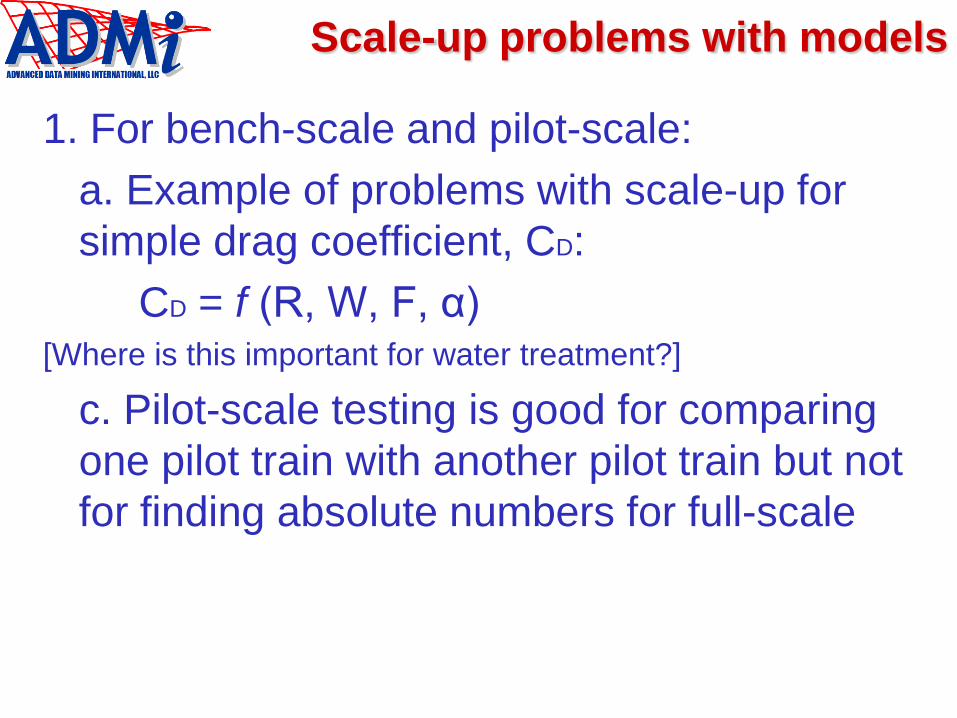
Scale-up problems with models

1. For bench-scale and pilot-scale:

a. Example of problems with scale-up for

simple drag coefficient, CD:

CD = f (R, W, F, α)[Where is this important for water treatment?]

c. Pilot-scale testing is good for comparing

one pilot train with another pilot train but not

for finding absolute numbers for full-scale

So what of models?

―Models are undeniably beautiful, and a man may

justly be proud to be seen in their company. But

they may have their hidden vices. The question is,

after all, not only whether they are good to look at,

but whether we can live happily with them.‖

--Abraham Kaplan, The Conduct of Inquiry

Another problem: chaotic behavior

• ―Deterministic evolution of a nonlinear system

which is between regular behavior and

stochastic behavior.” – Abarbanel

• ―The property that characterizes a dynamical

system in which most orbits exhibit sensitive

dependence.” – Lorenz

• ―Neither periodic or stochastic behaviors that

have structure in state/feature space, making

them somewhat predictable.‖– ADMi

Lorenz attractor shows problem

• Poster child of chaos

• Purely synthetic, derived from 3 equations

– dx/dt = -σx + σy

– dy/dt = -xz + rx – y

– dz/dt = xy – bz

signal3D delay plot

showing

“orbitals”

“extreme sensitivity to changes

in boundary conditions”

mode 1

mode 2

mode 1

mode 2

Chaos in Savannah River estuary

Savannah River salinity intrusion

measured

predicted

R2=0.88

low f SC 24-hr MWA

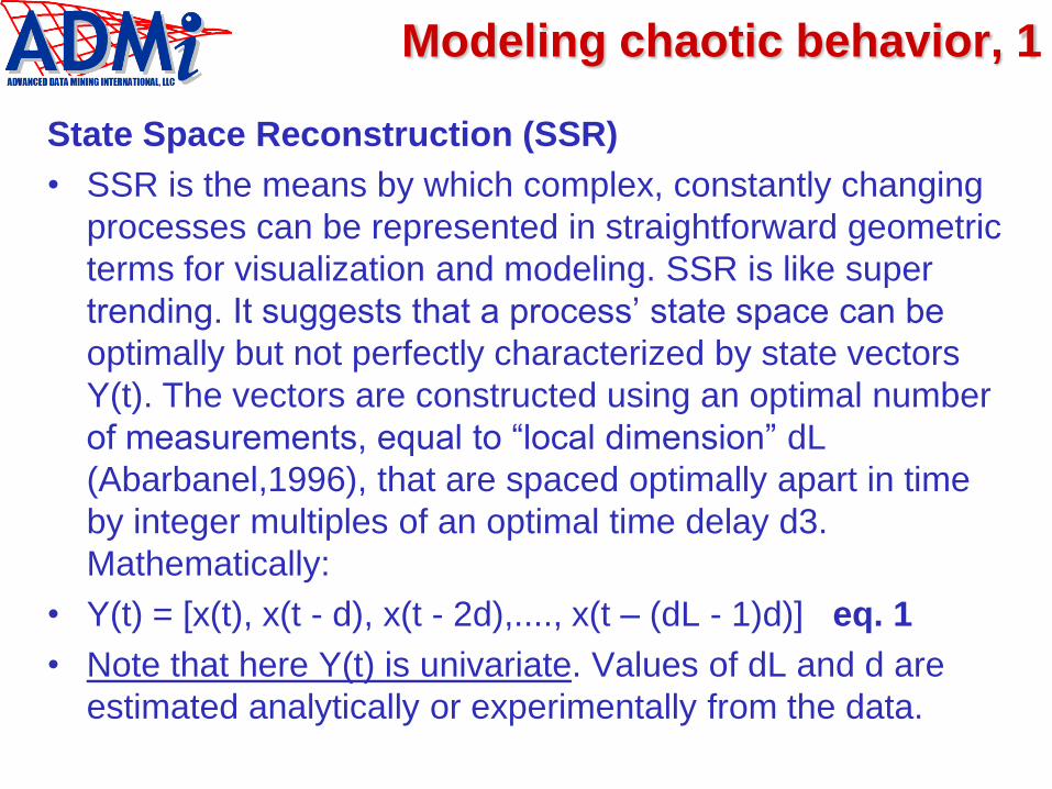
Modeling chaotic behavior, 1

State Space Reconstruction (SSR)

• SSR is the means by which complex, constantly changing

processes can be represented in straightforward geometric

terms for visualization and modeling. SSR is like super

trending. It suggests that a process’ state space can be

optimally but not perfectly characterized by state vectors

Y(t). The vectors are constructed using an optimal number

of measurements, equal to ―local dimension‖ dL

(Abarbanel,1996), that are spaced optimally apart in time

by integer multiples of an optimal time delay d3.

Mathematically:

• Y(t) = [x(t), x(t - d), x(t - 2d),...., x(t – (dL - 1)d)] eq. 1

• Note that here Y(t) is univariate. Values of dL and d are

estimated analytically or experimentally from the data.

Modeling chaotic behavior, 2

• For a multivariate process of k independent variables:

• Y(t) = {[x1(t), x1(t - d1),…, x1(t – (dL1 – 1)d1)],....,[xk(t),

xk(t - dk),…, xk(t – (dLk – 1)dk)]} eq. 2

• This provides each variable with its own dL and d. A further

generalization that provides non-fixed time delay spacing

for each variable:

• Y(t) = {[x1(t), x1(t - d1,1),…, x1(t – (dL1 – 1)d1,dL1-

1)],....,[xk(t), xk(t - dk,1),…, xk(t – (dLk – 1)dk,dLk-1]} eq. 3

• Determining the best variables xk to use, and properly

estimating dimensions dLk and time delays dk by analytical

or experimental means, helps to insure that a given

process can be successfully reconstructed.

The fundamental problem:

―The simple things you see are

all complicated.‖—Substitute,

Pete Townhsend

Consider modeling full-scale

system with full-scale system

1. Approach

a. Use data mining to extract information

contained in the full-scale data

b. Eliminates problems inherent in scale-up

issues

c. Chaotic behavior can be modeled

d. Systematic and objective approach to

optimizing information

Building Process

Models

A view of a general process

PHYSICAL

PROCESS

inputs

outputsx1

x2

x3

x4

x5

x6

x7

x8

y1

y2

y3

multiply periodicchaotic

stochastic

Causes of Variability• people

• configuration of controls

• raw water

• weather

• chemicals

• Outputs that are

predictable can then

be controlled

• Outputs that are

unpredictable cannot

be controlled

Relate variables with neural

networks

• Inspired by the Brain

– get complicated behaviors from lots of ―simple‖

interconnected devices - neurons and synapses

– non-linear, multivariate curve fitting

– models are synthesized from example data

• machine learning

x1

x2

x3

x4

x5

y1

y2

inputs outputs

ANNs produce response surfacesExample: Trihalomethanes Formation

no data

surface fitted by non-linear

ANN model represents normal

behavior

deviation from normal

better conditions?

CASE STUDY NO. 1—THM

AND HAA5 REDUCTION

Modeling chloroform

• Input = TURBFIN (MWA=4,t=-1), R2

ANN=0.47, RMSE=7.3

• +Input=COLORFIN (MWA=4), R2

ANN=0.60, RMSE=6.2

• +Input=TPFIN, R2ANN=0.74,

RMSE=5.0

R2ANN=0.74

same

TPFIN=32C

TPFIN=11C

CF higher

at high TP

Days when DBPs measured

Observations about chloroform

• Finished turbidity accounts for 47% of

variability in chloroform

• Finished turbidity + color accounts for 60%

• Finished turbidity + color + temperature

accounts for 74%

• Or, R2ANN = 0.74

• Recommend:

1) optimize turbidity removal—most

importantIs this counterintuitive?

2) optimize TOC removal

3D scatter plot

outlier

Modeling

BDM, Part 1

• Inputs = TURBFIN (t=-2) , COLORFIN (MWA=3), R2

ANN=0.24, RMSE=1.8


RMSE=1.2BDM far more sensitive to

TPFIN than TURBFIN &

COLORFIN

R2ANN=0.66

TPFIN=32C

TPFIN=11C


Observations regarding BDM

• Finished turbidity + finished color accounts

for 24% [very low correlation!]

• Finished turbidity + color + temperature

accounts for 66%

• Or, R2 = 0.66

• So, BDM is dominated by temperature

• Remove TURBFIN, add inputs = PRE-Cl2, R2

ANN=0.72, RMSE=1.1Modeling

BDM, Part 2

TPFIN=11C

COLORFIN=3.0TPFIN=11C

COLORFIN=1.0

TPFIN=32C

COLORFIN=3.0

TPFIN=32C

COLORFIN=1.0

BDM sensitivity

to PRE-Cl2 &

NH3 higher at

low TPFIN.

BDM higher at

higher

COLORFIN.

TP is dominant

effect.

Modeling TCA

• Input = TURBFIN (MWA=4,t=-3), R2

ANN=0.47, RMSE=5.5

• +Input=COLORFIN (MWA=4), R2

ANN=0.47, RMSE=5.5


RMSE=4.7

TPFIN=32C

TPFIN=11C

TCA less seasonal

than DCA

R2ANN=0.61


Observations modeling TCA

• Finished turbidity accounts for 47%

variability

• Finished turbidity + finished color accounts

for 47% [surprising, as color not capturing

precursors!]

• Finished turbidity + color + finished

temperature accounts for 61%

• Or, R2 = 0.61

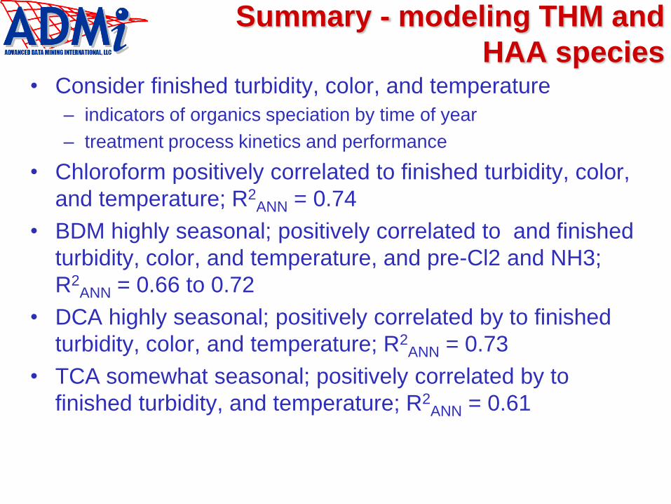
Summary - modeling THM and

HAA species• Consider finished turbidity, color, and temperature

– indicators of organics speciation by time of year

– treatment process kinetics and performance

• Chloroform positively correlated to finished turbidity, color,

and temperature; R2ANN = 0.74

• BDM highly seasonal; positively correlated to and finished

turbidity, color, and temperature, and pre-Cl2 and NH3;

R2ANN = 0.66 to 0.72

• DCA highly seasonal; positively correlated by to finished

turbidity, color, and temperature; R2ANN = 0.73

• TCA somewhat seasonal; positively correlated by to

finished turbidity, and temperature; R2ANN = 0.61

CASE STUDY NO. 2—THM

OPTIMIZATION

Conventional WTP case study Predict and ReduceTHM Formation

• Near real-time

predictions

• $ Savings by

optimizing use of

chemicals

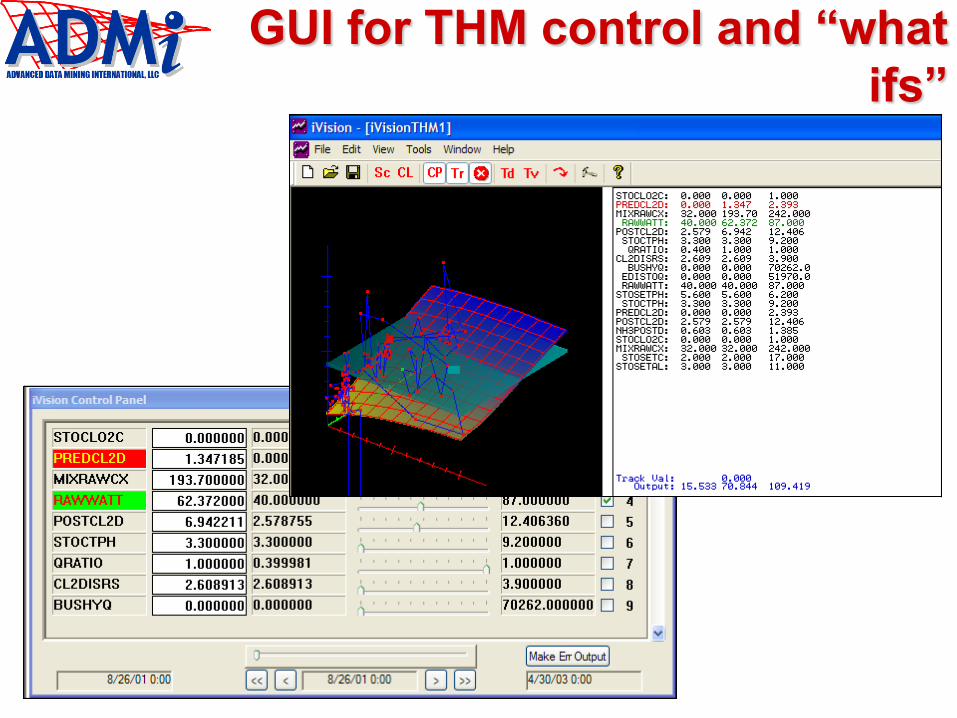
GUI for THM control and ―what

ifs‖

CASE STUDY NO. 3—

OPTIMIZE GENERAL

PROCESS

Determine Optimal TOC Removal

3D response surfaces for % TOC

removal• Unshown input settings

– R-TOC-BLNDCALC = 0

– R-PHXY = 0 (hist. avg. = 7.34)

– CLO2-H-BLNDCALC = 0.030 mg/l (hist. min.)

– COAGAID-X = 0.053 mg/l (hist. min.)

– COAG-X = 12.0 mg/l (hist. min.)

% TOC removal contour maps• Unshown input settings

– R-TOC-BLNDCALC = 0

– R-PHXY-C = 0 (hist. avg. = 7.34)

– CLO2-H-BLNDCALC = 0.030 mg/l (hist. min.)

– COAGAID-X = 0.053 mg/l (hist. min.)

– COAG-X = 12.0 mg/l (hist. min.)

Observations for % TOC removal

• Optimal coagulation pH = 6.5

• Coagulation aid = 0.05 mg/L (or < )

– However, coagulant aid does effect turbidity

• ClO2 = 0.8 mg/L

• Coagulant dose as function of [TOC]

Determine Optimal Turbidity

Removal

Total % turbidity removal

• System is robust in removal of turbidity regardless of source turbidity

levels; when source turbidity increases, % removal asymptotically

approaches –100%

• Goal is to minimize operating costs to meet water quality targets

Predict % filtration turbidity removal

• Unshown input settings

– R-TURB-BLNDCALC = 0

– Historical minimums

• CLO2-H-BLNDCALC = 0.030 mg/l

• COAGAID-T3456CALC = 0.057 mg/l

• COAG-T3456CALC = 12.0 mg/l

• FLTAID-T3456CALC = 0.0041 mg/l

Contour maps for turbidity filtration

– R-TURB-BLNDCALC = 0

– Historical mins

• CLO2-H-BLNDCALC = 0.030 mg/l

• COAGAID-T3456CALC = 0.057 mg/l

• COAG-T3456CALC = 12.0 mg/l

• FLTAID-T3456CALC = 0.0041 mg/l

Observations % filtration turbidity

removal

1. Turbidity removal through filtration is highly

sensitive to:

a. coagulant dose

b. chlorine dioxide dose

2. Turbidity removal through filtration is NOT

sensitive to filter polymer aid

3. Turbidity removal = f (sed. turbidity + ClO2 +

coagulant + coagulant aid); R2 = 0.75

4. Filter run times very low; recommend eliminating

filter polymer aid

5. Recommend side-by-side filter testing

CASE STUDY NO. 4—

MODELING TANK

NITRIFICATION

Days

Nea

rby

Ch

lori

ne

(mg

/l)

Ta

nk

Lev

el (

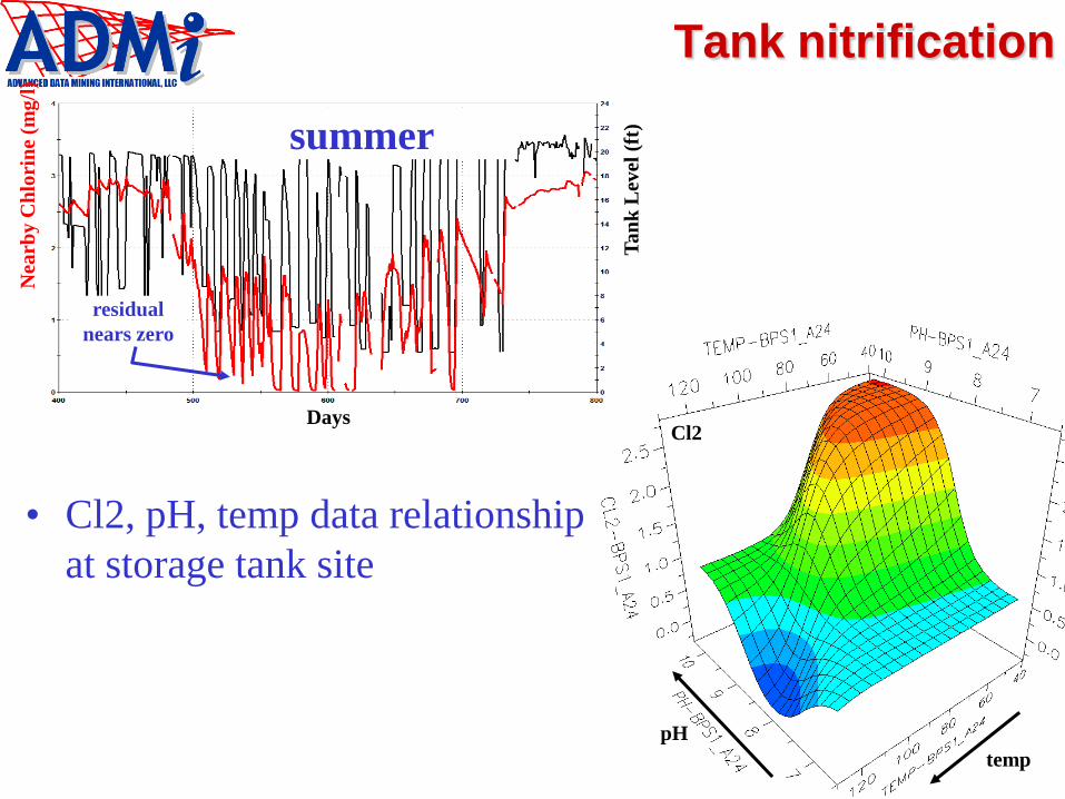
ft)summer

residual

nears zero

pH

temp

Cl2

• Cl2, pH, temp data relationship

at storage tank site

Tank nitrification

Observations about tank water

quality

• Nitrification demonstrated by loss of total

chlorine residual, lower pH, higher NO-2

• Total chlorine loss is pH sensitive

• Total chlorine loss is very temperature

dependent

– Nitrification rate increases exponentially above

approximately 80 F

• At pH > 9, loss of residual stabilizes

Questions

John B. Cook, PE

Advanced Data Mining Intl,

Greenville, SC

[email protected]

843.513.2130

www.advdmi.com

Modeling full scale-data(2)

Environment

Transcript of Modeling full scale-data(2)