Modeling Focused Beam

Propagation in scattering media

Janaka Ranasinghesagara, Ph.D.

Teaching Objectives

► The need for computational models of focused beam propagation in

scattering media

► Introduction to the principles and mathematical models underlying

focus beam propagation.

► Learn how fundamental concepts are applied to develop an efficient

focused beam propagation model.

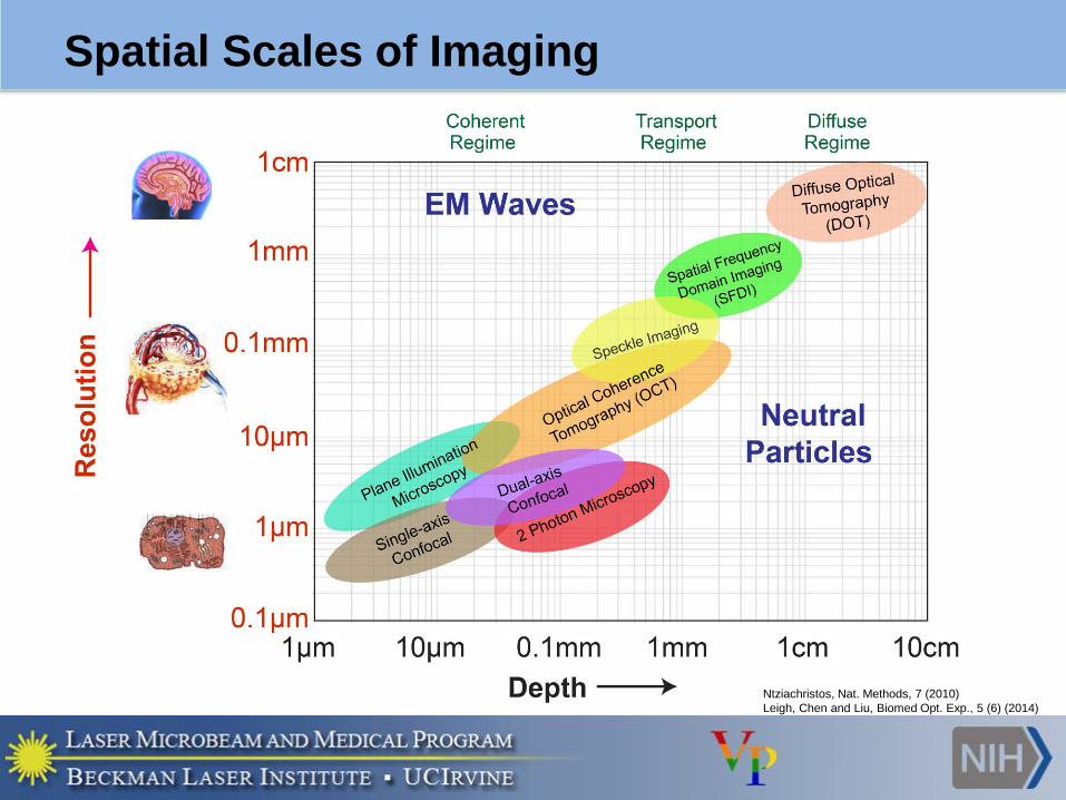
Spatial Scales of Imaging

Ntziachristos, Nat. Methods, 7 (2010)

Leigh, Chen and Liu, Biomed Opt. Exp., 5 (6) (2014)

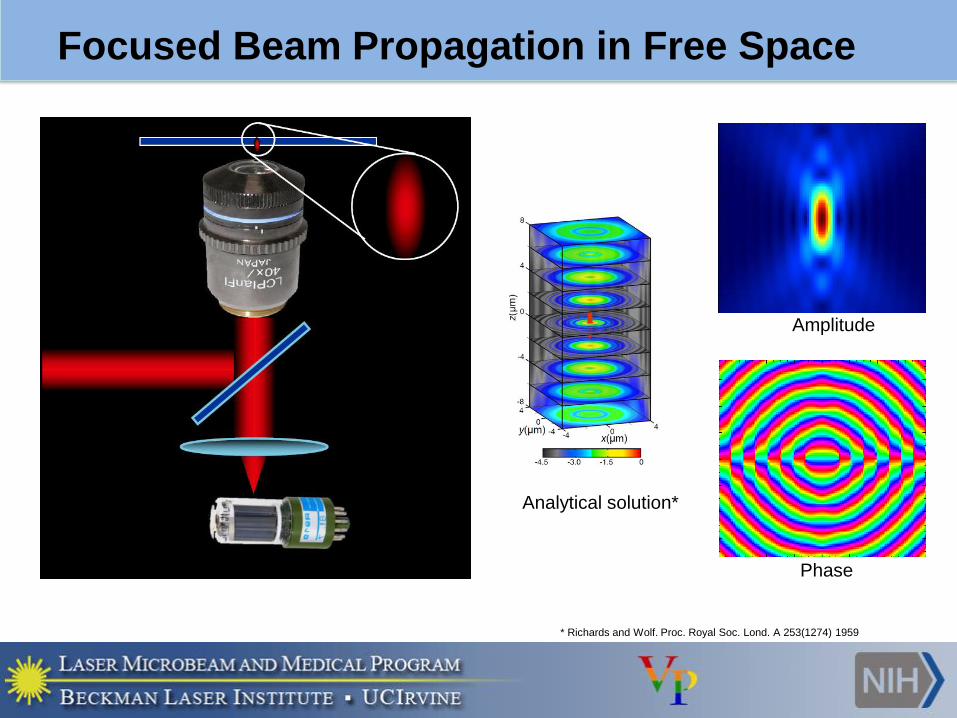
Focused Beam Propagation in Free Space

Analytical solution*

* Richards and Wolf. Proc. Royal Soc. Lond. A 253(1274) 1959

Amplitude

Phase

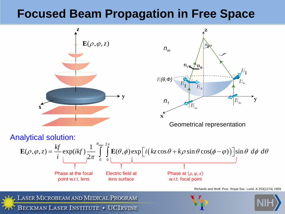
Focused Beam Propagation in Free Space

max 2

0 0

1( , , ) exp( ) ( , ) exp cos sin cos( ) sin

2

E E kf

z ikf i kz k d di

Phase at 𝜌, 𝜑, 𝑧w.r.t. focal point

Electric field at

lens surface

Phase at the focal

point w.r.t. lens

Richards and Wolf. Proc. Royal Soc. Lond. A 253(1274) 1959

Geometrical representation

Analytical solution:

max( , , )E z

Focused Beam Propagation in Scattering Media

• Scattering distorts the excitation volume

• Scattering is the main limiting factor for penetration depth in

microscopy

Existing Focused Beam Propagation Models

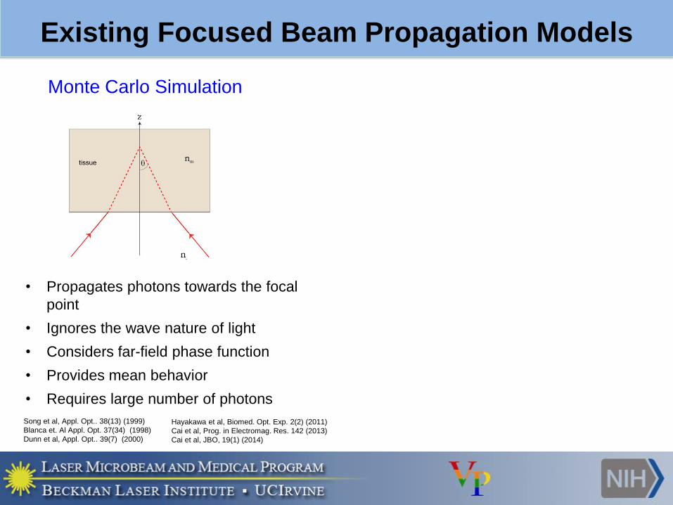
Monte Carlo Simulation

• Propagates photons towards the focal

point

• Ignores the wave nature of light

• Considers far-field phase function

• Provides mean behavior

• Requires large number of photons

Song et al, Appl. Opt.. 38(13) (1999)

Blanca et. Al Appl. Opt. 37(34) (1998)

Dunn et al, Appl. Opt.. 39(7) (2000)

Hayakawa et al, Biomed. Opt. Exp. 2(2) (2011)

Cai et al, Prog. in Electromag. Res. 142 (2013)

Cai et al, JBO, 19(1) (2014)

Existing Focused Beam Propagation Models

Monte Carlo Simulation

• Propagates photons towards the focal

point

• Ignores the wave nature of light

• Considers far-field phase function

• Provides mean behavior

• Requires large number of photons

Song et al, Appl. Opt.. 38(13) (1999)

Blanca et. Al Appl. Opt. 37(34) (1998)

Dunn et al, Appl. Opt.. 39(7) (2000)

Hayakawa et al, Biomed. Opt. Exp. 2(2) (2011)

Cai et al, Prog. in Electromag. Res. 142 (2013)

Cai et al, JBO, 19(1) (2014)

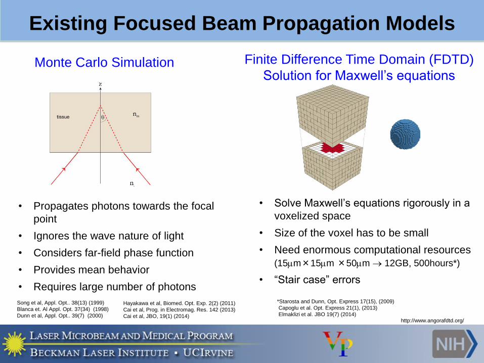
Finite Difference Time Domain (FDTD)

Solution for Maxwell’s equations

• Solve Maxwell’s equations rigorously in a

voxelized space

• Size of the voxel has to be small

• Need enormous computational resources

(15m×15m ×50m 12GB, 500hours*)

• “Stair case” errors

*Starosta and Dunn, Opt. Express 17(15), (2009)

Capoglu et al. Opt. Express 21(1), (2013)

Elmaklizi et al. JBO 19(7) (2014)http://www.angorafdtd.org/

►Electromagnetic wave

►Maxwell’s equations

►Plane wave solution to Maxwell’s

equations

►Properties of plane wave

Key Concepts, Equations and Properties

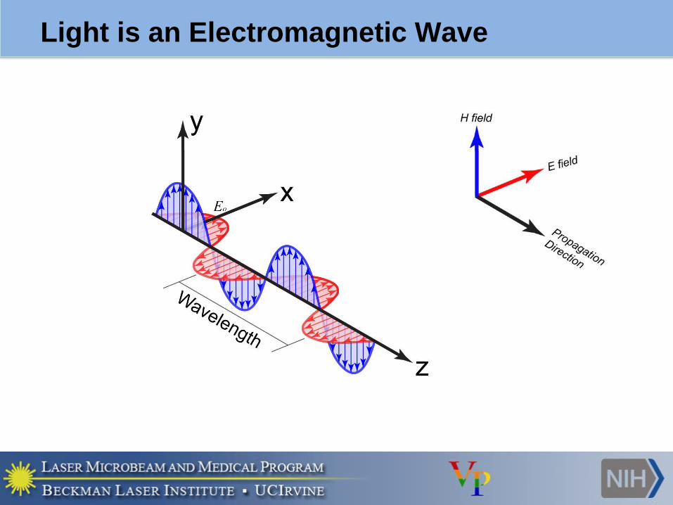
Light is an Electromagnetic Wave

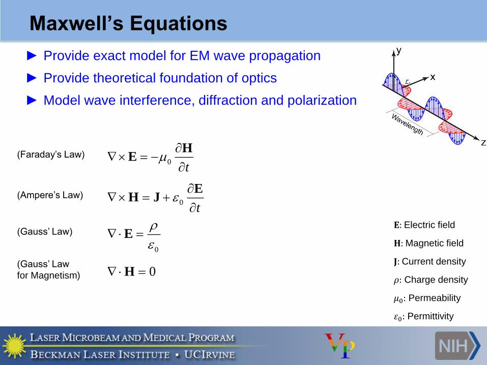
Maxwell’s Equations

► Provide exact model for EM wave propagation

► Provide theoretical foundation of optics

► Model wave interference, diffraction and polarization

0t

HE

0t

EH J

0

E

0 H

(Faraday’s Law)

(Gauss’ Law)

(Gauss’ Law

for Magnetism)

(Ampere’s Law)

𝐄: Electric field

𝐇: Magnetic field

𝐉: Current density

𝜌: Charge density

𝜇0: Permeability

𝜀0: Permittivity

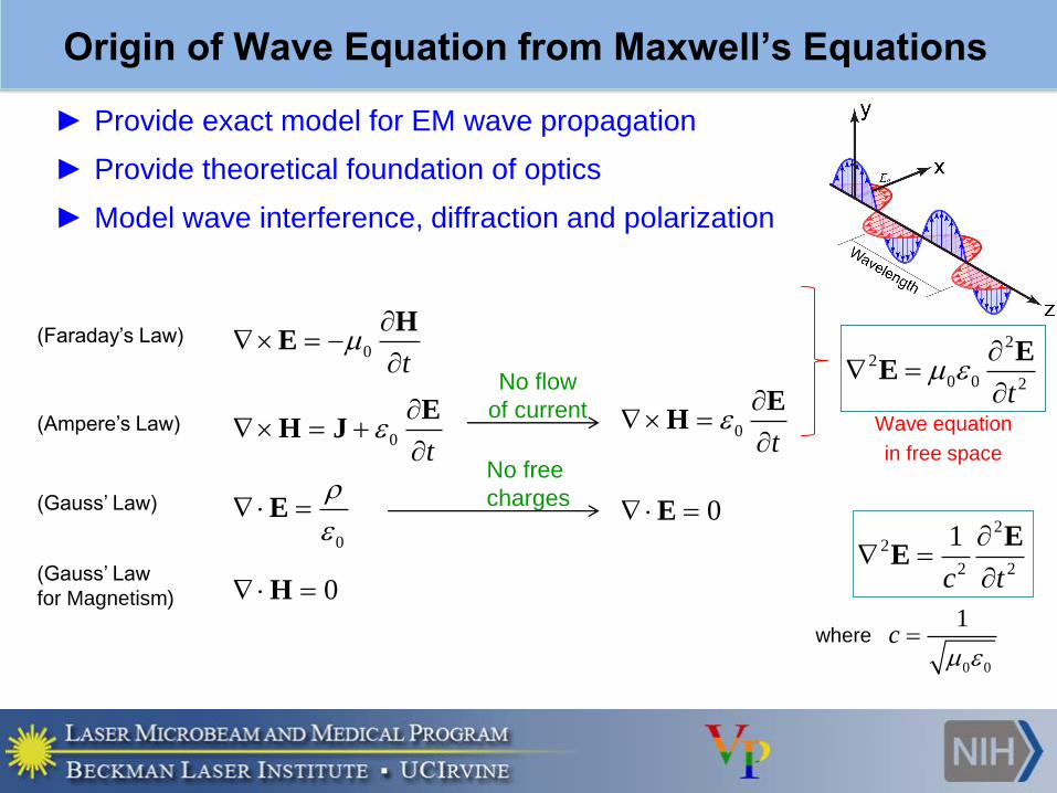
Origin of Wave Equation from Maxwell’s Equations

► Provide exact model for EM wave propagation

► Provide theoretical foundation of optics

► Model wave interference, diffraction and polarization

0t

HE

0t

EH J

0

E

0 H

(Faraday’s Law)

(Gauss’ Law)

(Gauss’ Law

for Magnetism)

(Ampere’s Law) 0t

EH

0 E

No free

charges

No flow

of current

22

0 0 2t

EE

Wave equation

in free space

22

2 2

1

c t

EE

where

0 0

1c

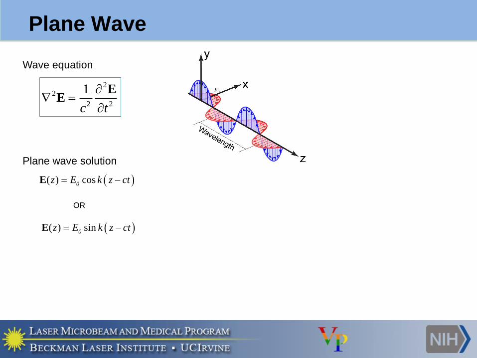
Plane Wave

22

2 2

1

c t

EE

Plane wave solution

( ) cos E 0z E k z ct

( ) sin E 0z E k z ct

OR

Wave equation

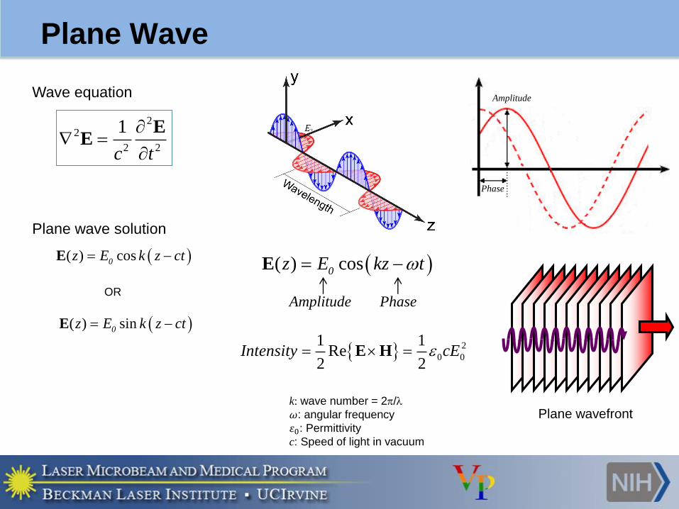
Plane Wave

( ) cos E 0z E kz t

2

0 0

1 1Re

2 2Intensity cE E H

k: wave number = 2/

𝜔: angular frequency

𝜀0: Permittivity

c: Speed of light in vacuum

Amplitude Phase

Amplitude

Phase

Plane wavefront

22

2 2

1

c t

EE

Plane wave solution

( ) cos E 0z E k z ct

( ) sin E 0z E k z ct

OR

Wave equation

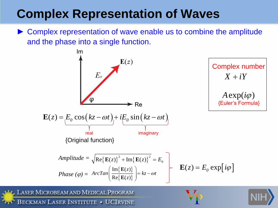
Complex Representation of Waves

( ) cos sin E 0 0z E kz t iE kz t

Amplitude =

Im ( )

Re ( )

zArcTan kz t

z

E

EPhase () =

( ) exp0z E iE

{Euler’s Formula}

2 2

0Re ( ) Im ( ) E Ez z E

real imaginary

► Complex representation of wave enable us to combine the amplitude

and the phase into a single function.

{Original function}

X iY

Complex number

exp( )A i

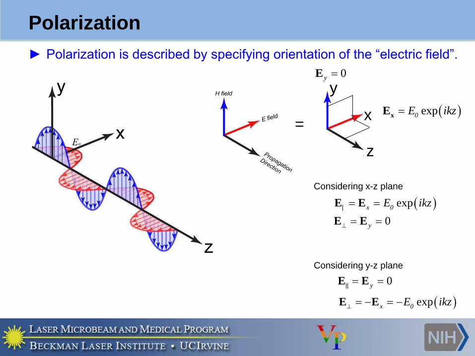
Polarization

► Polarization is described by specifying orientation of the “electric field”.

Considering x-z plane

exp E Ex 0E ikz

0 E E y

Considering y-z plane

0 E E y

exp E Ex 0E ikz

exp0

E ikzx

E

0y E

=

z

y

x

Focused Beam Propagation in Free Space

max 2

0 0

1( , , ) exp( ) ( , ) exp cos sin cos( ) sin

2

E E kf

z ikf i kz k d di

Phase at 𝜌, 𝜑, 𝑧w.r.t. focal point

Electric field at

lens surface

Phase at the focal

point w.r.t. lens

Richards and Wolf. Proc. Royal Soc. Lond. A 253(1274) 1959

Geometrical representation

Analytical solution:

max( , , )E z

►Mie Solution to Maxwell’s Equations

(commonly known as Mie Theory)

►Mie Simulator GUI

Plane Wave Incident on a Spherical Scatterer

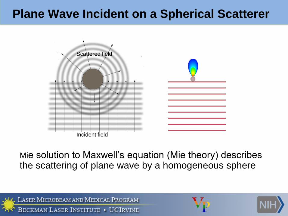
Plane Wave Incident on a Spherical Scatterer

Incident field

Scattered field

Mie solution to Maxwell’s equation (Mie theory) describes the scattering of plane wave by a homogeneous sphere

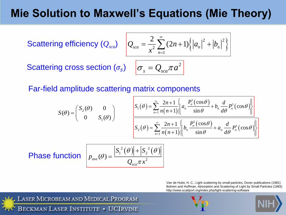
Mie Solution to Maxwell’s Equations (Mie Theory)

Van de Hulst, H. C., Light scattering by small particles, Dover publications (1981)

Bohren and Huffman, Absorption and Scattering of Light by Small Particles (1983)

http://www.scattport.org/index.php/light-scattering-software

2 2

21

2(2 1)

sca n n

n

Q n a bx

Scattering efficiency (Qsca)

Scattering cross section (𝜎𝑠)2 s scaQ a

Far-field amplitude scattering matrix components

1

1

1

1

cos2 1cos

1 sin

n

n n n

n

Pn dS a b P

n n d

1

1

2

1

cos2 1cos

1 sin

n

n n n

n

Pn dS b a P

n n d

Phase function 2 2

1 2

2( )

ave

sca

S Sp

Q x

2

1

( ) 0( )

0 ( )

SS

S

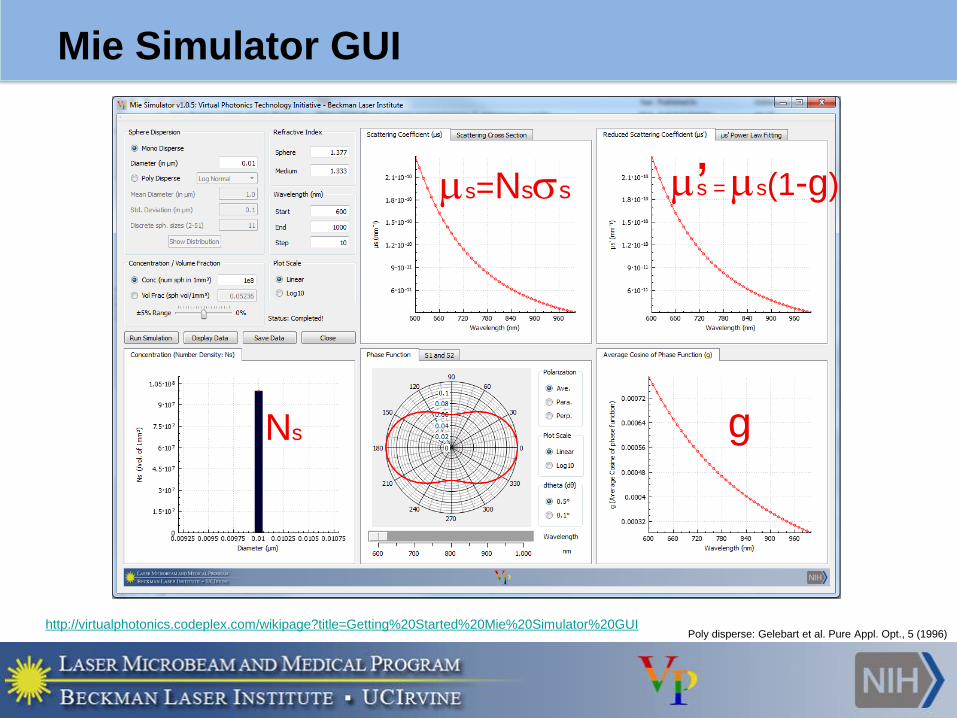
Mie Simulator GUI

s=Nss

g

’

Ns

s = s(1-g)

Poly disperse: Gelebart et al. Pure Appl. Opt., 5 (1996)http://virtualphotonics.codeplex.com/wikipage?title=Getting%20Started%20Mie%20Simulator%20GUI

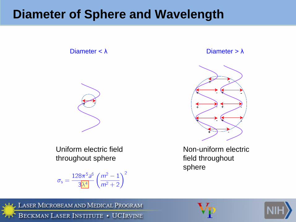
Diameter of Sphere and Wavelength

Diameter < λ Diameter > λ

Uniform electric field

throughout sphere

Non-uniform electric

field throughout

sphere

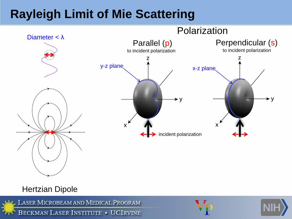
Rayleigh Limit of Mie Scattering

Parallel (p) to incident polarization

Perpendicular (s)to incident polarization

Polarization

Hertzian Dipole

0

180

0

180

x-z planey-z plane

Diameter < λ

Mie Simulator GUI Mie Simulator GUI

incident polarization

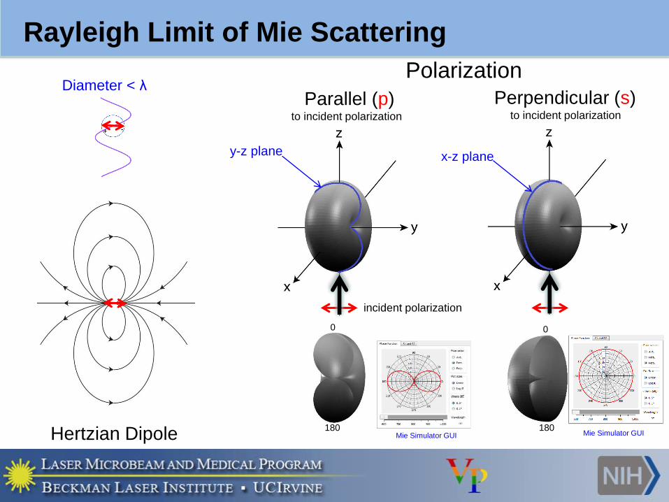
Rayleigh Limit of Mie Scattering

Parallel (p) to incident polarization

Perpendicular (s)to incident polarization

Polarization

Hertzian Dipole

0

180

0

180

x-z planey-z plane

Diameter < λ

Mie Simulator GUI Mie Simulator GUI

incident polarization

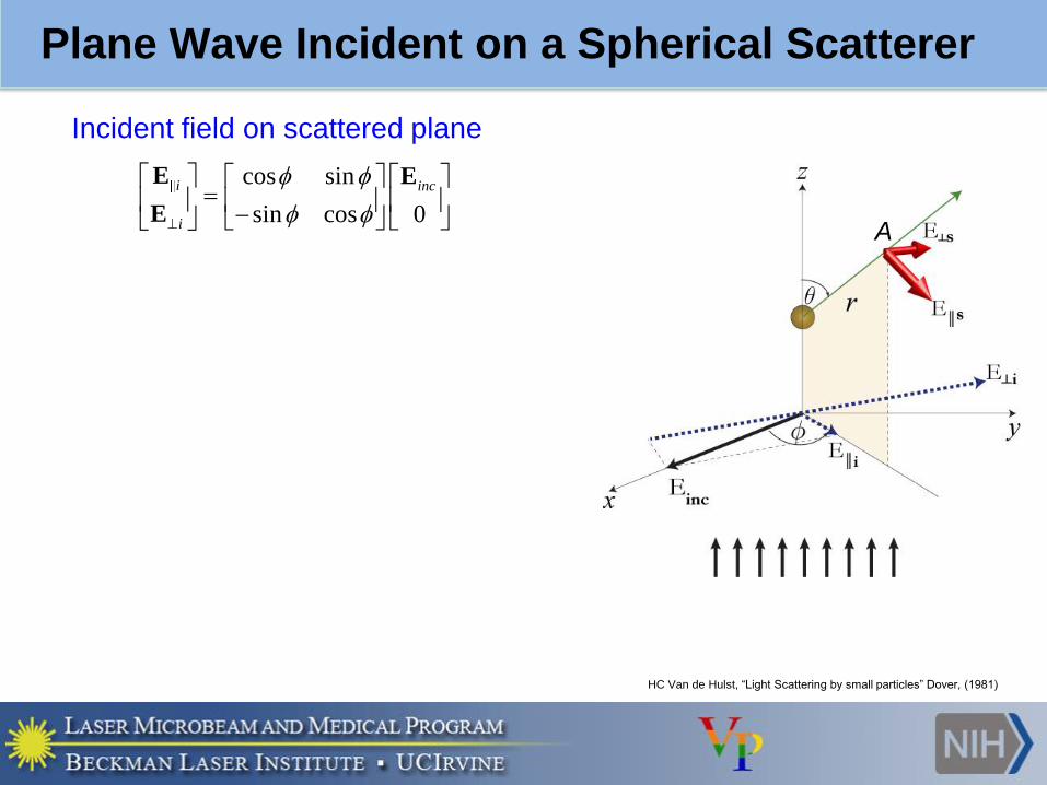
Plane Wave Incident on a Spherical Scatterer

A

HC Van de Hulst, “Light Scattering by small particles” Dover, (1981)

cos sin

sin cos 0

E E

E

i inc

i

Incident field on scattered plane

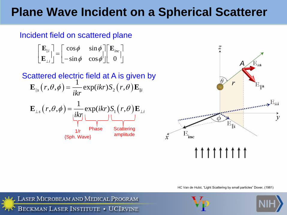
Scattered electric field at A is given by

2

1, , exp( ) , E Es ir ikr S r

ikr

A

HC Van de Hulst, “Light Scattering by small particles” Dover, (1981)

cos sin

sin cos 0

E E

E

i inc

i

Incident field on scattered plane

1

1, , exp( ) , E Es ir ikr S r

ikr

Phase Scattering

amplitude1/r

{Sph. Wave}

Plane Wave Incident on a Spherical Scatterer

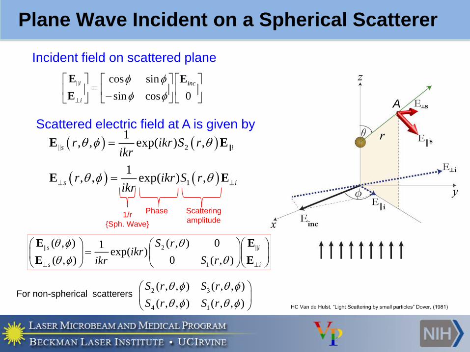
Scattered electric field at A is given by

2

1, , exp( ) , E Es ir ikr S r

ikr

A

HC Van de Hulst, “Light Scattering by small particles” Dover, (1981)

cos sin

sin cos 0

E E

E

i inc

i

Incident field on scattered plane

1

1, , exp( ) , E Es ir ikr S r

ikr

Phase Scattering

amplitude

2

1

( , ) ( , ) 01exp( )

( , ) 0 ( , )

E E

E E

s i

s i

S rikr

S rikr

1/r

{Sph. Wave}

For non-spherical scatterers 2 3

4 1

( , , ) ( , , )

( , , ) ( , , )

S r S r

S r S r

Plane Wave Incident on a Spherical Scatterer

►Huygens-Fresnel (HF) Principle

►Focused beam as a summation of plane

waves

►Constructive and destructive interference

of HF waves

►HF-WEFS model algorithm

An Efficient Focused Beam Propagation Model

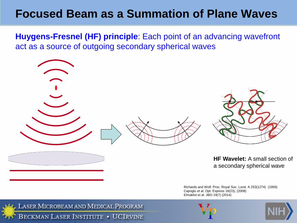
Focused Beam as a Summation of Plane Waves

Richards and Wolf. Proc. Royal Soc. Lond. A 253(1274) (1959)

Capoglu et al. Opt. Express 16(23), (2008)

Elmaklizi et al. JBO 19(7) (2014)

Huygens-Fresnel (HF) principle: Each point of an advancing wavefront

act as a source of outgoing secondary spherical waves

HF Wavelet: A small section of

a secondary spherical wave

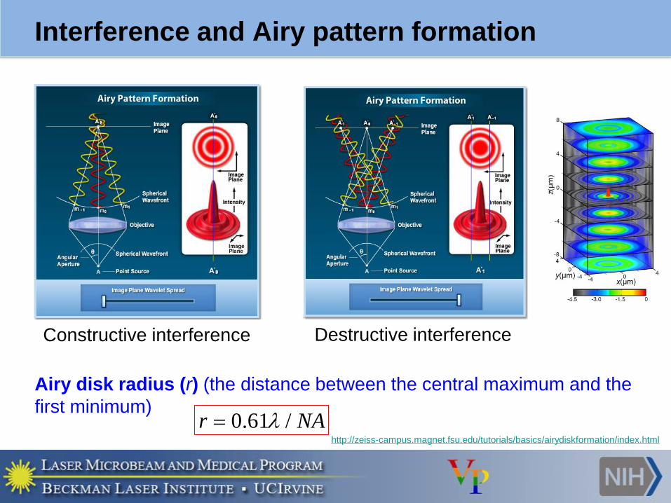
Interference and Airy pattern formation

Airy disk radius (r) (the distance between the central maximum and the

first minimum)0.61 /r NA

Constructive interference Destructive interference

http://zeiss-campus.magnet.fsu.edu/tutorials/basics/airydiskformation/index.html

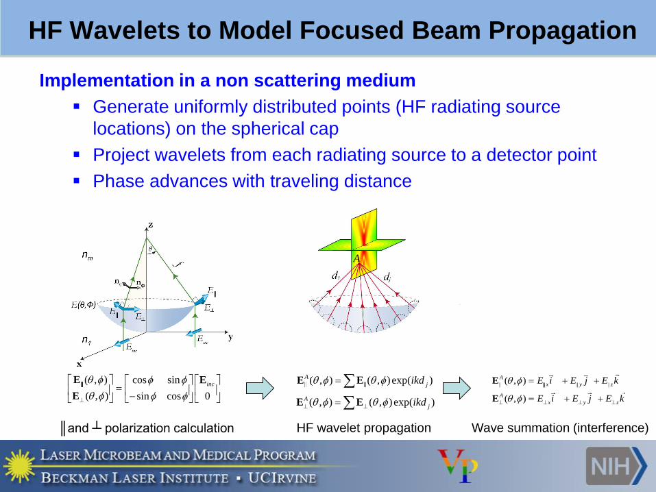
HF Wavelets to Model Focused Beam Propagation

Implementation in a non scattering medium

▪ Generate uniformly distributed points (HF radiating source

locations) on the spherical cap

▪ Project wavelets from each radiating source to a detector point

▪ Phase advances with traveling distance

( , ) cos sin

( , ) sin cos 0

E E

E

inc ( , ) ( , ) exp( )A

jikd E E

( , ) ( , ) exp( )A

jikd

E E

A

( , )

( , )

E

E

A

x y z

A

x y z

E i E j E k

E i E j E k

║and ┴ polarization calculation HF wavelet propagation Wave summation (interference)

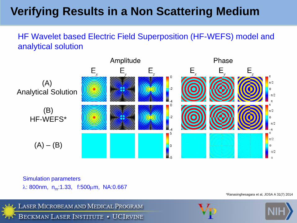
HF Wavelet based Electric Field Superposition (HF-WEFS) model and

analytical solution

(A)

Analytical Solution

(B)

HF-WEFS*

Simulation parameters

: 800nm, nm:1.33, f:500m, NA:0.667

(A) – (B)

Verifying Results in a Non Scattering Medium

*Ranasinghesagara et al, JOSA A 31(7) 2014

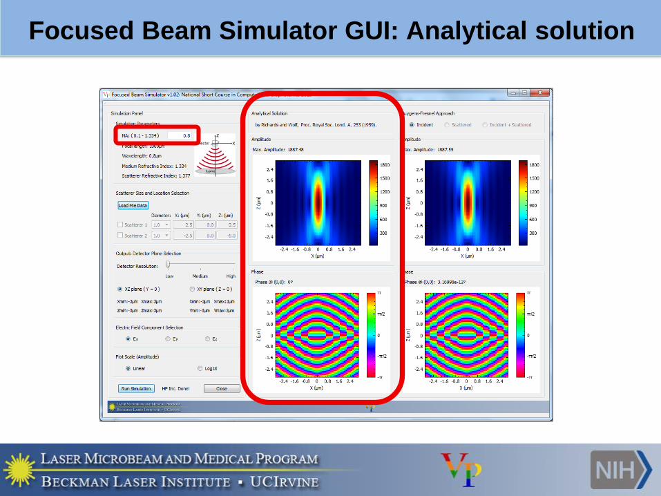
Focused Beam Simulator GUI: Analytical solution

Focused Beam Simulator GUI: Huygens-Fresnel Approach

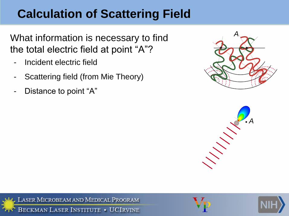
Calculation of Scattering Field

A

What information is necessary to find

the total electric field at point “A”?

- Incident electric field

- Scattering field (from Mie Theory)

- Distance to point “A”

A

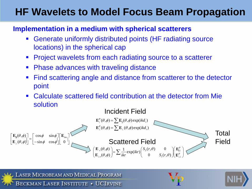
HF Wavelets to Model Focus Beam Propagation

Implementation in a medium with spherical scatterers

▪ Generate uniformly distributed points (HF radiating source

locations) in the spherical cap

▪ Project wavelets from each radiating source to a scatterer

▪ Phase advances with traveling distance

▪ Find scattering angle and distance from scatterer to the detector

point

▪ Calculate scattered field contribution at the detector from Mie

solution

( , ) cos sin

( , ) sin cos 0

E E

E

inc

( , ) ( , ) exp( )P

iikd E E

( , ) ( , ) exp( )P

iikd

E E

2

1

( , ) ( , ) 01exp( )

( , ) 0 ( , )

Ps i

Ps i

S rikr

S rikr

E E

E E

Total

Field

Incident Field

Scattered Field

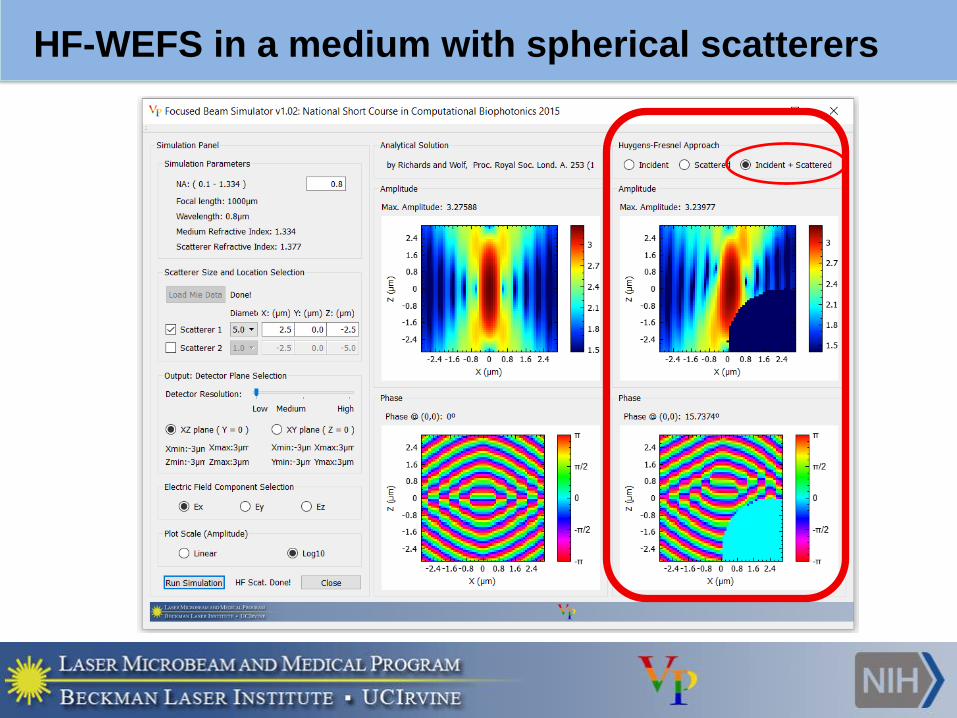
HF-WEFS in a medium with spherical scatterers

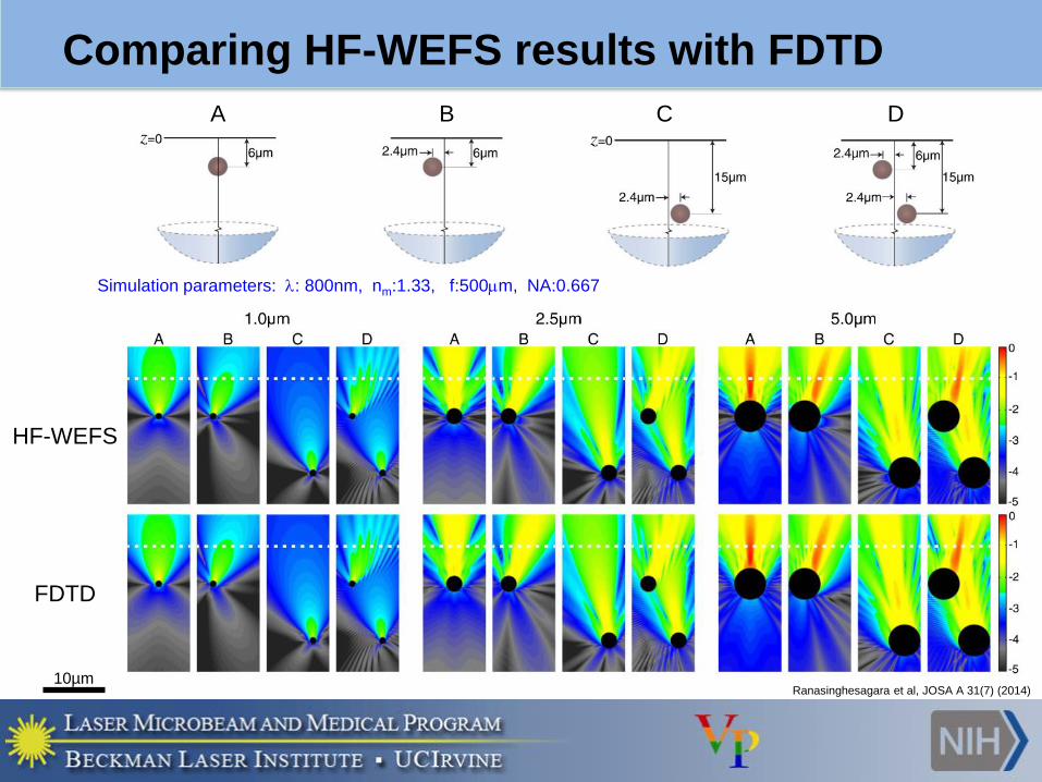
Comparing HF-WEFS results with FDTD

Simulation parameters: : 800nm, nm:1.33, f:500m, NA:0.667

Ranasinghesagara et al, JOSA A 31(7) (2014)

A B C D

HF-WEFS

FDTD

10µm