
Modeling Energy Production of Solar Thermal Systems and ...
133
University of Wisconsin Milwaukee UWM Digital Commons eses and Dissertations December 2012 Modeling Energy Production of Solar ermal Systems and Wind Turbines for Installation at Corn Ethanol Plants Elizabeth Ehrke University of Wisconsin-Milwaukee Follow this and additional works at: hps://dc.uwm.edu/etd Part of the Oil, Gas, and Energy Commons is esis is brought to you for free and open access by UWM Digital Commons. It has been accepted for inclusion in eses and Dissertations by an authorized administrator of UWM Digital Commons. For more information, please contact [email protected]. Recommended Citation Ehrke, Elizabeth, "Modeling Energy Production of Solar ermal Systems and Wind Turbines for Installation at Corn Ethanol Plants" (2012). eses and Dissertations. 29. hps://dc.uwm.edu/etd/29
Transcript of Modeling Energy Production of Solar Thermal Systems and ...

University of Wisconsin MilwaukeeUWM Digital Commons
Theses and Dissertations
December 2012
Modeling Energy Production of Solar ThermalSystems and Wind Turbines for Installation at CornEthanol PlantsElizabeth EhrkeUniversity of Wisconsin-Milwaukee
Follow this and additional works at: https://dc.uwm.edu/etdPart of the Oil, Gas, and Energy Commons
This Thesis is brought to you for free and open access by UWM Digital Commons. It has been accepted for inclusion in Theses and Dissertations by anauthorized administrator of UWM Digital Commons. For more information, please contact [email protected].
Recommended CitationEhrke, Elizabeth, "Modeling Energy Production of Solar Thermal Systems and Wind Turbines for Installation at Corn Ethanol Plants"(2012). Theses and Dissertations. 29.https://dc.uwm.edu/etd/29

MODELING ENERGY PRODUCTION OF SOLAR THERMAL
SYSTEMS AND WIND TURBINES FOR INSTALLATION AT CORN
ETHANOL PLANTS
by
Elizabeth Ehrke
A Thesis Submitted in
Partial Fulfillment of the
Requirements for the Degree of
Master of Science
in Engineering
at
The University of Wisconsin-Milwaukee
December 2012

ii
ABSTRACT
MODELING ENERGY PRODUCTION OF SOLAR THERMAL SYSTEMS AND WIND TURBINES FOR INSTALLATION AT CORN ETHANOL PLANTS
by
Elizabeth Ehrke
The University of Wisconsin-Milwaukee, 2012 Under the Supervision of Dr. John Reisel
Nearly every aspect of human existence relies on energy in some way. Most of
this energy is currently derived from fossil fuel resources. Increasing energy demands
coupled with environmental and national security concerns have facilitated the move
towards renewable energy sources. Biofuels like corn ethanol are one of the ways the
U.S. has significantly reduced petroleum consumption. However, the large energy
requirement of corn ethanol limits the net benefit of the fuel. Using renewable energy
sources to produce ethanol can greatly improve its economic and environmental benefits.
The main purpose of this study was to model the useful energy received from a solar
thermal array and a wind turbine at various locations to determine the feasibility of
applying these technologies at ethanol plants around the country. The model calculates
thermal energy received from a solar collector array and electricity generated by a wind
turbine utilizing various input data to characterize the equipment. Project cost and energy
rate inputs are used to evaluate the profitability of the solar array or wind turbine. The
current state of the wind and solar markets were examined to give an accurate
representation of the economics of each industry.

iii
Eighteen ethanol plant locations were evaluated for the viability of a solar thermal
array and/or wind turbine. All ethanol plant locations have long payback periods for
solar thermal arrays, but high natural gas prices significantly reduce this timeframe.
Government incentives will be necessary for the economic feasibility of solar thermal
arrays. Wind turbines can be very profitable for ethanol plants in the Midwest due to
large wind resources. The profitability of wind power is sensitive to regional energy
prices. However, government incentives for wind power do not significantly change the
economic feasibility of a wind turbine. This model can be used by current or future
ethanol facilities to investigate or begin the planning process for a solar thermal array or
wind turbine. The model is meant to aide in the planning stages of a renewable energy
project, and advanced investigation will be needed to move forward with that project.

iv
TABLE OF CONTENTS
LIST OF FIGURES ............................................................................................................ v LIST OF TABLES ........................................................................................................... viii
LIST OF ABBREVIATIONS ............................................................................................. x LIST OF SYMBOLS ........................................................................................................ xii
CHAPTER 1: INTRODUCTION ....................................................................................... 1 CHAPTER 2: BACKGROUND ......................................................................................... 5
2.1 Introduction ............................................................................................................... 5 2.2 Ethanol Background .................................................................................................. 5 2.3 Energy and Economic Concerns ............................................................................. 13 2.4 Wind Energy ........................................................................................................... 20 2.5 Solar Thermal Energy ............................................................................................. 27 2.6 Summary ................................................................................................................. 31
CHAPTER 3: MODELING TECHNIQUE AND APPROACH ...................................... 32 3.1 Introduction to the Model ....................................................................................... 32 3.2 Energy Use by Ethanol Plant .................................................................................. 34 3.3 Resource and Meteorological Inputs ...................................................................... 37 3.4 Calculating Wind Power Generated ........................................................................ 41 3.5 Calculating the Solar Energy Collected .................................................................. 51 3.6 Project Costs and Savings ....................................................................................... 60 3.7 Evaluations and Comparisons of Ethanol Plant Locations ..................................... 66 3.8 Summary ................................................................................................................. 67
CHAPTER 4: MODEL RESULTS AND ANALYSIS .................................................... 68 4.1 Introduction ............................................................................................................. 68 4.2 Verifying the Solar Energy Model .......................................................................... 68 4.3 Evaluating Flat Plate and Evacuated Tube Arrays ................................................. 70 4.4 Evaluating Model Results for Solar Thermal Projects ........................................... 73 4.5 Verifying the Wind Energy Model ......................................................................... 85 4.6 Evaluating Model Results for Wind Projects .......................................................... 87 4.7 Summary ................................................................................................................. 98
CHAPTER 5: CONCLUSIONS AND RECOMMENDATIONS .................................... 99
REFERENCES ............................................................................................................... 104 APPENDIX A ................................................................................................................. 109
APPENDIX B ................................................................................................................. 115

v
LIST OF FIGURES
2.1 U.S. Map of Corn Production and Ethanol Plant Locations 7
2.2 World Energy Consumption 1990-2035 15
2.3 Annual World Oil Prices in Three Cases, 1980-2035 16
2.4 RFS Mandated Consumption of Renewable Fuels, 2009-2022 17
2.5 EISA 2007 RFS Credits Earned in Selected Years, 2010-2035 18
2.6 U.S. Wind Speed Map at 80 Meters 25
2.7 U.S. Installed Wind Capacity 25
2.8 World Renewable Electricity Generation by Source, 2005-2035 26
2.9 U.S. Map of Solar Thermal Resources 29
2.10 Flat Plate and Evacuated Tube Collector Diagram 29
3.1 Ethanol Plant Inputs 34
3.2 Resource and Meteorological Inputs 38
3.3 Wind Inputs 41
3.4 Power Coefficient as a Function of Tip Speed Ratio 43
3.5 Power Curve of 2MW Turbine 44

vi
3.6 Wind Turbine Installed Cost 48
3.7 Installed Cost for 1982-2012 Wind Projects 49
3.8 Wind Outputs 50
3.9 Solar Inputs 52
3.10 Solar Outputs 59
3.11 Price Inputs 62
3.12 Cost and Savings Outputs 64
3.13 Map of 18 Ethanol Locations Used in Model 66
4.1 Modeled Gross Area and SPF Solar Collector Efficiency 69
4.2 Modeled Aperture Area and SPF Collector Efficiency 70
4.3 Flat Plate and Evacuated Tube Comparison,18 Locations, Ti=30oC 71
4.4 Flat Plate and Evacuated Tube Comparison, 18 Locations, Ti=60oC 72
4.5 Ethanol Plant Capacities and Percent Sift to Solar Heating 74
4.6 Cumulative Cost Savings for Flat Plate Array 75
4.7 Monthly Useful Energy Production, Flat Plate 76
4.8 Cumulative Cost Savings Using State Natural Gas Rates, TX and CA 77
4.9 Cumulative Cost Savings Using State Natural Gas Rates, AZ and MO 78
vii
4.10 Cumulative Cost Savings for Natural Gas Rate Increase, AZ 80
4.11 Cumulative Cost Savings for Different Installed Costs, NE 81
4.12 Average Wind Speed and Yearly Electricity Production, 18 Locations 88
4.13 Plant Capacities and Percent Shift to Wind Power 89
4.14 Monthly Electricity Generation, 1.5MW Turbine 90
4.15 Cumulative Cost Savings, 1.5MW Turbine 91
4.16 Cumulative Cost Savings Using State Electricity Rates, CA and WY 92
4.17 Cumulative Cost Savings Using Government Incentives, KS 93
4.18 Cumulative Cost Savings Using Government Incentives, WI 94

viii
LIST OF TABLES
3.1 Average Efficiency Values for Solar Thermal Collectors 58
4.1 Model inputs for flat plate and evacuated tube collector 81
4.2 Comparison of model outputs for monthly and yearly data inputs 82
4.3 Sate natural gas rates and payback period modeled for flat plate collector 83
4.4 Model inputs for standard wind turbine 85
4.5 Model outputs for wind turbine 86
4.6 Model price inputs and installed cost output 91
4.7 Payback period and yearly cost savings using state electricity rate 95
4.8 Comparison of model outputs for monthly and yearly input data 97
A.1 Meteorological and resource data for Logansport, IN 109
A.2 Meteorological and resource data for Gibson City, IL 109
A.3 Meteorological and resource data for Cambria, WI 110
A.4 Meteorological and resource data for Marshall, MN 110
A.5 Meteorological and resource data for Watertown, SD 110
A.6 Meteorological and resource data for Richardton, ND 110

ix
A.7 Meteorological and resource data for Arthur, IA 111
A.8 Meteorological and resource data for St. Joseph, MO 111
A.9 Meteorological and resource data for Sutherland, NE 111
A.10 Meteorological and resource data for Torrington, WY 111
A.11 Meteorological and resource data for Burley, ID 112
A.12 Meteorological and resource data for Yuma, CO 112
A.13 Meteorological and resource data for Russell, KS 112
A.14 Meteorological and resource data for Arkalon, KS 112
A.15 Meteorological and resource data for Plainview, TX 113
A.16 Meteorological and resource data for Imperial Valley, CA 113
A.17 Meteorological and resource data for Stockton, CA 113
A.18 Meteorological and resource data for Maricopa, AZ 113
A.19 Ethanol plant coordinates and solar panel tilt angle 114
B.1 Average U.S. and state natural gas prices 116
B.2 Average U.S. and state electricity prices 117

x
LIST OF ABBREVIATIONS
AC Alternating Current
ACE American Coalition for Ethanol
AWEA American Wind Energy Association
Btu British thermal unit
CFDC Clean Fuels Development Coalition
DDG Dry distillers grain
DOE United States Department of Energy
DSIRE Database of State Incentives for Renewables & Efficiency
DWG Distillers wet grain
EIA U.S. Energy Information Administration
EPA Environmental Protection Agency
ESIA Energy Independence and Security Act
GHG Greenhouse gas
GWEC Global Wind Energy Council
IEA International Energy Agency
IEA SHC International Energy Agency’s Solar Heating and Cooling
Programme
IPCC Intergovernmental Panel on Climate Change
ITC Investment Tax Credit
MMBtu Million British thermal units
MTBE Methyl Tertiary Butyl Ether

xi
NASA National Aeronautics and Space Administration
NREL National Renewable Energy Laboratory
O&M Operational and maintenance
ODEC Organization for Economic Co-operation and Development
POWER Prediction of Worldwide Energy Resource Project
PPA Power Purchase Agreement
PTC Production Tax Credit
RFA Renewable Fuel Association
RFS Renewable Fuel Standard
RPM Revolutions per Minute
SSE Surface meteorology and Solar Energy
SPF Institut für Solartechnik (Institute for Solar Technology)
TSR Tip speed ratio
USDA United States Department of Agriculture
xii
LIST OF SYMBOLS
a1 Solar efficiency coefficient 1 (W/m2K)
a2 Solar efficiency coefficient 2 (W/m2K2)
Aa Aperture area of solar collector (m2)
Ac Total area of solar collector (m2)
As Swept area of wind turbine (m2)
Cf Capacity factor of wind turbine
Cfa Actual capacity factor of wind turbine
CP Coefficient of power of wind turbine
Cpa Actual coefficient of power of wind turbine
Cpd Design coefficient of power of wind turbine
CSs Cumulative cost savings for solar array
CSw Cumulative cost savings for wind turbine
DR Diameter of rotor (m)
EBtu Energy generated by wind turbine (MMBtu/yr)
Ew Energy generated by wind turbine (kWh/yr)
Ewt Theoretical energy generated by ideal wind turbine (kWh/yr)
ER Ethanol plant electricity requirement (kWh/gal-ethanol)
FR(τα) Collector heat removal factor times transmittance-absorptance product
FRUL Collector heat removal factor times collector heat loss coefficient
(W/m2-oC)
G Solar irradiation (W/m2)

xiii
Gt Solar insolation on a tilted surface (kWh/m2/day)
Gta Yearly average solar insolation on a tilted surface (kWh/m2/day)
Hday Number of hours per day (h/day)
Hy Number of hours in one year (h/yr)
ICsc Installed cost per square foot of solar collector ($/ft2)
ICwt Installed cost per kilowatt of wind turbine ($/kW)
Lf Load factor of solar array
MWB Boiler makeup water requirement (gal-water/gal-ethanol)
MWtotal Total ethanol plant makeup water requirement
nE Annual percent increase of electricity price
nNB Annual percent increase of natural gas price
Nc Number of collectors in solar array
Nd Number of days
Np Number of solar panels
PC Ideal power capacity of a wind turbine (kW)
Pw Power output of wind turbine (kW)
PC Plant capacity (MGY)
PPs Simple payback period for solar array (years)
PPw Simple payback period for wind turbine (years)
QAE Total heating requirement per gallon ethanol (Btu/gal-ethanol)
𝑄!"!""# Energy to cook ethanol (Btu/gal-ethanol)
𝑄!"! Energy to distill ethanol (Btu/gal-ethanol)
QMW Total heating requirement of the boiler makeup water (Btu/gal-ethanol)

xiv
QTotal Total heating requirement of ethanol production (MMBtu)
Qu Useful solar energy (MJ/yr)
Qut Useful solar energy (MMBtu/yr)
RE Electricity rate ($/kWh)
RNG Natural gas rate ($/MMBtu)
SE Yearly electricity cost savings ($/yr)
SNG Yearly natural gas cost savings ($/yr)
SC Solar array total installed cost ($)
Ta Average ambient temperature (oC)
Ti Average inlet temperature of the working fluid (oC)
Tm Mean temperature of working fluid in collector (oC)
Vw Wind speed (m/s)
Va Actual wind speed at wind turbine hub height (m/s)
Vd Design wind speed for wind turbine (m/s)
WC Wind turbine total installed cost ($)
ηa Efficiency of solar array based on aperture area
ηap Efficiency of panel based on aperture area
ηc Efficiency of solar array based on gross collector area
ηcp Efficiency of panel based on gross collector area
ηo SPF solar efficiency coefficient
ηspf Solar panel efficiency using SPF coefficients
ρa Density of air (kg/m3)
%SMW Percent shift from natural gas to solar energy for the boiler makeup water

xv
%Sw Percent shift from conventional electricity to wind energy
%Ss Percent shift from natural gas to solar energy
%WB Percent of makeup water used by the boiler

1
CHAPTER 1: INTRODUCTION
Energy is a global concern. There are limited sources of conventional energy like
fossil fuels, and alternatives are generally expensive, limited in capacity, or represent
technology still in need of development. Growing concerns over global climate change
and energy security have lead to expanded use of renewable energy sources like fuel
ethanol, wind power, and solar energy. These technologies are expected to grow in
capacity to meet rising global energy requirements to help offset fossil fuel use. One of
the benefits of wind and solar energy is that it is available to everyone. Unlike a coal-
fired power plant that must be continually managed, a wind turbine can generate energy
in a cornfield with little supervision. Solar thermal installations require slightly more
oversight, but the use of modern control systems makes a solar thermal array easy to
manage.
Both wind power and solar energy can be used to offset the copious fossil fuel
consumption at an ethanol plant. One of the main drawbacks of corn ethanol is the
energy requirement to produce the fuel. Ethanol is considered a renewable fuel because
it is made from corn that uses the sun’s energy to grow, but the current production
methods of ethanol represent a non-renewable process. Increasing the amount of
renewable energy used for the production of ethanol will reduce fossil fuel use, decrease
greenhouse gas emissions, and ultimately reduce the ethanol plant’s energy costs.
The economics of a wind or solar energy project is not as straightforward as it
may seem. There are many factors that determine the economic feasibility of a
renewable energy project. Wind and solar resources vary widely across the country and

2
not every location is an ideal candidate for either technology. The type and size of the
equipment influence costs and potential energy savings. The current cost of energy plays
a major role in the financial advantage of a renewable energy project as well. All of these
factors make it difficult to give a good estimate for the initial costs, payback period, and
cost savings of a wind turbine or solar thermal system. General assumptions about wind
and solar energy are not applicable to a wide range of locations and project specifications.
The main purpose of this project is to create a model that can be used to evaluate
the feasibility of installing a wind turbine or solar thermal array at a corn ethanol plant.
The model can be used with plant-specific information to accurately estimate the useful
energy produced by a wind turbine and solar array at that location. Cost estimates for the
renewable energy installation along with the current price of natural gas and electricity
are then used to find the payback period and cost savings of each project. Numerous
variables can be changed to simulate different conditions for the renewable energy
technology, energy prices, and government incentives. This allows a wide range of
projects to be considered by the same model. It also enables the user to compare several
project options or different financial circumstances.
The estimated energy output of the model was verified by using experimental and
operational data for solar thermal panels and utility-scale wind turbines. Experimental
test data from the Institute for Solar Technology (SPF 2012) was used to compare the
model outputs to the real performance of the average solar thermal panel. Wind turbine
model outputs were compared to the averaged yearly output of hundreds of large-scale
wind turbines in the U.S. for 2011 (Wiser and Bolinger 2012).

3
The model was then used to assess the solar and wind resources at 18 different
U.S. ethanol plant locations. The economic feasibility of a solar thermal array and a wind
turbine was evaluated for each plant. The locations were chosen to represent a wide
variety of conditions to find the best areas for wind power and solar energy systems.
Various inputs were changed to determine the effects on payback period and cost savings.
Current federal tax incentives were also considered to determine their financial influence
on wind and solar projects. Realistic conditions were chosen to represent an accurate
estimate of costs and energy savings. Recommendations are then given for the best areas
for the application of solar energy and wind power.
This project continues the work of Kumar (2009), in which he created a model for
the energy requirements of a dry mill ethanol plant. Numerous design characteristics of
an ethanol plant can be entered to determine the natural gas requirements of a dry mill
corn ethanol plant. The ethanol model was also verified for its accuracy. The energy
requirement output for a specific corn ethanol plant from Kumar’s model can be used as
an input for this model to determine the percent shift to solar energy. Kumar’s model
also calculates the payback period and cost savings of a solar and wind project. His solar
and wind calculations are limited due to few design inputs and inadequate information to
help guide the user on realistic values for the solar energy and wind power calculations.
The wind calculations were not based on the available equipment on the market. Instead
of using a turbine of known dimensions, the dimensions were calculated depending on
the percent shift to wind power. This created a problem, because there are only certain
dimensions commercially available and wind turbine prices are based on design size not
actual power generated. The model created for this project improves the methods for

4
calculating useful solar energy and wind power. This project takes Kumar’s research
even further by not only creating a model, but also using that model to evaluate solar and
wind resources at ethanol plants across the country.
The renewable energy market is quickly growing and is expected to continue
expanding due to decreasing equipment prices, energy security concerns, and
environmental policy. A growing market means lower costs and better technology. This
indicates that wind and solar installations cost less and perform better than past
equipment. The current state of the solar thermal and wind industries is discussed in the
following chapters. Market projections for fossil fuels and renewable energy are also
included to show what the future of energy and energy costs might look like in the next
20 years.
Ethanol, wind power, and solar energy will all be a part of the energy matrix over
the next 20 years. Using wind and solar energy to produce ethanol can increase ethanol’s
sustainability and reduce overall energy costs. Not only can these renewable energy
resources save money, but they can also contribute to America’s goals of reducing fossil
fuel use, decreasing greenhouse gas emissions, and increasing energy security.

5
CHAPTER 2: BACKGROUND
2.1 Introduction
As the world economies advance, the demand for energy continues to increase.
Many agree that fossil fuels alone will not be able to sustain this level of consumption.
Fossil fuels like petroleum, coal, and natural gas must soon give way to greener
technologies like ethanol, wind, and solar energy. It is imperative that economic analysis
be made available to ease this transition from the old to the new age of energy. Though
we are most likely more than a half century away from depleting our fossil fuel resources
(Fay and Golomb 2012), action must be taken now to avoid energy shortages later.
Ethanol, wind, and solar energy will not be the only solution to the energy problem, but
they provide a viable option to reduce fossil fuel use right now.
The following sections will examine relevant historical and predictive market
information to characterize the current and future state of conventional and renewable
energy sources. Fuel ethanol, wind power, and solar energy are described in detail to
provide general background information and illustrate how each technology fits into the
U.S. energy market. Global energy and economic issues are briefly discussed as well.
The main focus is to provide background information for the study of the feasibility of
wind and solar installations at ethanol plants to reduce fossil fuel consumption.
2.2 Ethanol Background
Ethanol has been used for years as a fuel additive as a way to reduce gasoline
consumption, raise the octane level of fuel, and reduce pollution (CFDC 2010). Ethanol

6
is a clean burning, biodegradable fuel additive that acts as an oxidizer to facilitate a more
complete combustion of gasoline. Most of the ethanol produced in the U.S. comes from
corn crop in the Midwest. Cellulosic ethanol and advanced biofuel production have
shown promising advantages over corn ethanol for reducing greenhouse gas (GHG)
emissions and energy inputs, but obstacles still exist to large-scale development of this
technology. Since much of the energy contained in corn and cellulosic materials comes
from the sun, these are considered renewable fuels. One of the main reasons corn ethanol
is not completely renewable is the energy required to cook and distill the corn feedstock.
Producing ethanol requires process heat and electricity is needed to run the plant. Over
90% of U.S. facilities use natural gas for process heat (RFA 2012a) and use electricity
generated mainly from coal and natural gas. Reducing fossil fuel use in the production of
ethanol will make the process more sustainable.
The majority of ethanol plants are located throughout the Midwest where corn is
most plentiful. This ensures adequate supply and reduces transportation costs between
the farm and the ethanol production facility. A map of U.S. corn production and ethanol
plant locations is shown in Figure 2.1. Some of the ethanol plants located in areas
seemingly devoid of corn crop actually have corn production, but the corn crop was not
estimated for this figure. In addition, there are several plants that use feedstock other
than corn. About 90% of the ethanol plants in the U.S. use the dry mill process to
produce ethanol from corn (RFA 2012a). This study focuses on corn ethanol produced
from dry mill plants using natural gas for process heat. The wind and solar resources at
the current locations of ethanol plants will be used to assess the viability of using these
renewable energy sources.

7
Another advantage to placing ethanol plants near farmland is the proximity to
livestock. The main co-product of ethanol plants, distillers grains, is sold as an additive
to livestock feed. Wet and dry distillers grains have high protein content and are used in
animal feed for the dairy, beef, swine, and poultry industries. If the ethanol plant is close
enough to the livestock farm, the co-products can be sold as wet distillers grains, which
significantly reduces the energy required to dry the grains for transportation. In 2011,
ethanol co-products accounted for 12% of net corn use in the U.S., which amounted to
39.4 million metric tons of livestock feed (RFA 2012a). The corn used to produce
Figure 2.1: U.S. map of ethanol plant locations as of March 2008 and estimated number of bushels of corn produced in 2011 (USDA 2011).
Corn for Grain 2011Production by County and Location of Ethanol Plants
as of March 8, 2012
Note: The depicted ethanol plants use corn or other feedstock.Data Sources: U.S. Department of Agriculture, National Agricultural Statistics Service."USA Plants." Ethanol Producer Magazine, March. 2012. http://www.ethanolproducer.com/plants/listplants/USA/
Corn Production (Bushels)Not Estimated < 1,000,000 1,000,000 - 4,999,999 5,000,000 - 9,999,999 10,000,000 - 14,999,999 15,000,000 - 19,999,999 20,000,000 +
Ethanol PlantsProducingUnder Construction
8
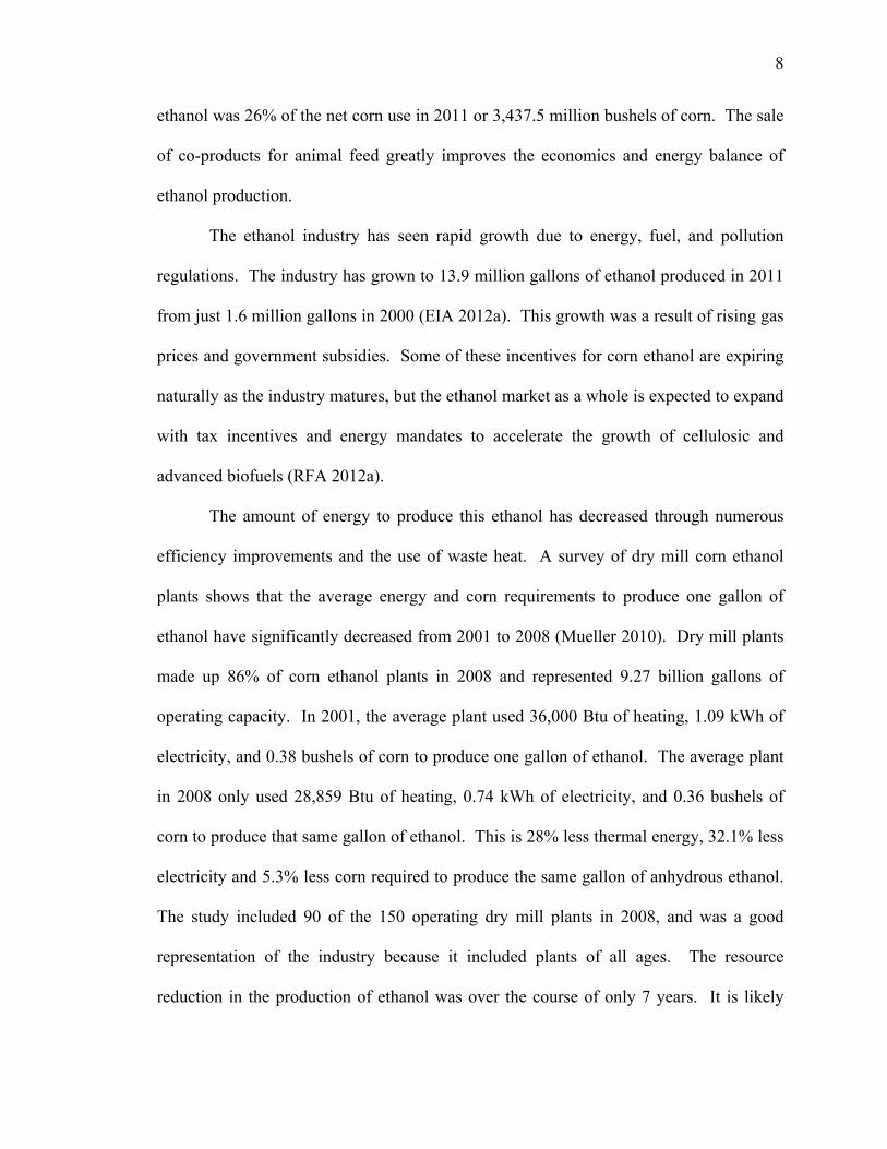
ethanol was 26% of the net corn use in 2011 or 3,437.5 million bushels of corn. The sale
of co-products for animal feed greatly improves the economics and energy balance of
ethanol production.
The ethanol industry has seen rapid growth due to energy, fuel, and pollution
regulations. The industry has grown to 13.9 million gallons of ethanol produced in 2011
from just 1.6 million gallons in 2000 (EIA 2012a). This growth was a result of rising gas
prices and government subsidies. Some of these incentives for corn ethanol are expiring
naturally as the industry matures, but the ethanol market as a whole is expected to expand
with tax incentives and energy mandates to accelerate the growth of cellulosic and
advanced biofuels (RFA 2012a).
The amount of energy to produce this ethanol has decreased through numerous
efficiency improvements and the use of waste heat. A survey of dry mill corn ethanol
plants shows that the average energy and corn requirements to produce one gallon of
ethanol have significantly decreased from 2001 to 2008 (Mueller 2010). Dry mill plants
made up 86% of corn ethanol plants in 2008 and represented 9.27 billion gallons of
operating capacity. In 2001, the average plant used 36,000 Btu of heating, 1.09 kWh of
electricity, and 0.38 bushels of corn to produce one gallon of ethanol. The average plant
in 2008 only used 28,859 Btu of heating, 0.74 kWh of electricity, and 0.36 bushels of
corn to produce that same gallon of ethanol. This is 28% less thermal energy, 32.1% less
electricity and 5.3% less corn required to produce the same gallon of anhydrous ethanol.
The study included 90 of the 150 operating dry mill plants in 2008, and was a good
representation of the industry because it included plants of all ages. The resource
reduction in the production of ethanol was over the course of only 7 years. It is likely

9
that energy usage and corn requirements will continue to decrease moderately as data
from newer plants are considered and existing plants incorporate energy saving
equipment and procedures.
The U.S. government and the Department of Energy (DOE) have been long time
supporters of increased production of fuel ethanol. The DOE succinctly sums up this
support through their biofuels mission statement:
The U.S. Department of Energy (DOE) is committed to advancing
technological solutions to promote and increase the use of clean, abundant,
affordable, and domestically- and sustainably-produced biofuels to
diversify our nation’s energy sources, reduce greenhouse gas emissions,
and reduce our dependence on oil (DOE 2008).
They stress the importance of continued development of biofuels such as ethanol in order
to meet the growing energy demand instead of relying on volatile foreign energy markets.
Not only does ethanol reduce oil imports, but also reduces GHG emissions and creates
American jobs.
Opponents of ethanol claim that it pollutes more than gasoline, but the DOE states
that the average life cycle of ethanol production, when compared to the life cycle of
gasoline production, significantly reduces greenhouse gas emissions. The average GHG
reduction of corn ethanol compared to gasoline was 19% in a DOE report (2008). This
value is dramatically increased when cleaner energy sources are used. Using natural gas
for process heating reduces lifecycle GHG emissions by 28-39% according to Wang, Wu,
and Huo (2007). Liska et al. (2008) show that GHG emissions can be reduced by 48-
59% when modern farming methods, production practices and co-product sales are

10
considered. Cellulosic ethanol production can reduce GHG emissions by 86% if biomass
is used for process heating (DOE 2008). The use of renewable energy sources for the
production of corn ethanol will further reduce lifecycle GHG emissions when compared
to gasoline.
The assertions of the DOE can be corroborated by Farrell et al. (2006) study that
examined 6 reports and created 3 of their own models of the energy life cycle of ethanol
to determine parameters used, assumptions made, and then standardize them using a new
evaluation technique to reproduce their results to within a half percent. They found that
the calculations are highly sensitive to the assumptions made in the parameters of the
study, boundaries of the calculations, and differences in the various types of fossil fuels.
They argue that the two studies that reported a negative energy balance for the ethanol
life cycle misrepresented key variables in their calculations and ignored the energy
consumption of the co-products of ethanol production. The largest disparities between
the studies stem from the treatment of co-products that replace items like corn and
soybean meal in animal feed, which inherently take energy to produce. There are several
limiting factors to the study due to large differences in reported energy consumption,
however the best estimate for corn ethanol is that it reduces petroleum use by about 95%
and reduces GHG emissions by 13%. These values are similar to the data reported by the
DOE. Farrell et al.’s study also found a dramatic environmental advantage to cellulosic
ethanol, but concluded more research is needed to investigate the feasibility of large-scale
cellulosic ethanol production. The study also found that agriculture practices account for
34-44% of GHG emissions and 45-85% of the petroleum inputs to the production of corn
ethanol. Concluding that improving agriculture practices could significantly improve the

11
energy balance and GHG emissions in ethanol production. The article suggests that
advancements in sustainable agriculture and cellulosic ethanol will grow the biofuels
industry to ultimately reduce energy consumption and reduce negative environmental
impacts.
There is some concern about the sustainability of increasing corn crop and other
ethanol feedstock to meet the demand for increased biofuels. The DOE and the U.S.
Department of Agriculture (USDA) conducted a study that concluded the U.S. could
grow enough biomass to replace about 30% of current gasoline use without drastic
changes to current land use (Perlack 2005). The report asserts this is more than adequate
to meet the standards set by the Energy Independence and Security Act of 2007, which
requires that 36 billion gallons of renewable transportation fuels be in use by 2022.
Advancing technologies are increasing crop output per acre and reducing resource inputs.
The act also caps the amount of corn ethanol to limit strain on the corn market. It is clear
that the DOE has high hopes for cellulosic ethanol and its role in the future of ethanol.
Many ethanol opponents claim ethanol has a negative energy balance (Pimentel
2003) (Keeney and DeLuca 1992), but others specifically disprove these claims
(Shapouri et al. 2002) (Farrel et al. 2006). The DOE (2008) reports that gasoline takes
about 1.23 Btu to produce per 1 Btu of energy delivered. This is called a negative energy
balance because it takes more non-renewable energy to produce than is delivered by the
gasoline. Corn ethanol energy balance is about 0.73 Btu in per Btu delivered, while
cellulosic ethanol energy balance is about 0.1 Btu in per Btu delivered. The report shows
that gasoline is produced using energy derived almost solely from petroleum products,
while ethanol uses almost entirely coal and natural gas. Natural gas and coal are more

12
abundant resources and are domestically available. Studies that show a negative energy
balance typically ignore the co-products that are a result of ethanol production (Farrell et
al. 2006) (Shapouri et al. 2002). The co-products from ethanol can be used as animal
feed and replace other ingredients that take energy to produce. The studies also site
technological advancements that have improved agricultural practices. Better farming
methods have increased energy efficiency and reduced pollution. All of these factors
lead to a positive energy balance for corn ethanol, which consumes less non-renewable
energy than gasoline.
Another myth the DOE would like to dispel is the notion that 10% ethanol-
gasoline blends significantly reduce the fuel economy of the vehicle. Since modern cars
are designed to run on a 10% blend, there is no measurable reduction in vehicle fuel
economy (ACE 2005). Since ethanol is generally less expensive than gasoline the slight
reduction in fuel efficiency with ethanol blended gasoline is offset by the lower cost.
Knoll (2009) concludes that 10% ethanol blends reduce fuel efficiency by 3-4%.
Gasoline burns more completely when using an oxygenate like ethanol, which reduces
some harmful pollutants. Ethanol replaced MTBE as a fuel oxygenate after MTBE was
found to contaminate groundwater (DOE 2012). There is some disagreement about
ethanol’s ability to reduce harmful tailpipe emissions and reduce pollution (Niven 2004),
but Knoll (2009) finds that most agree 10% ethanol blends reduce carbon monoxide by
15% and non-methane hydrocarbons by 12%. Even though tailpipe emissions are only
moderately reduced, ethanol currently displaces 485 million barrels of imported oil a year
(RFA 2012a). This supports the U.S. economy and reduces fuel use required to transport
the oil to America. The DOE asserts that further advancement of agriculture practices
13
combined with increased use of renewable energy sources in the production of ethanol
will continue to reduce GHG emissions. It is clear that although ethanol may have some
drawbacks, ethanol is reducing GHG emissions and petroleum use. By substituting fossil
fuel with renewable energy sources in the production of ethanol, the negative
environmental impacts can be dramatically reduced.
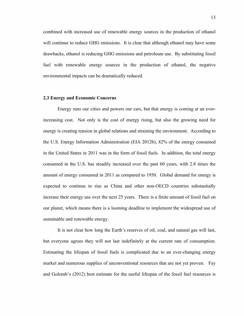
2.3 Energy and Economic Concerns
Energy runs our cities and powers our cars, but that energy is coming at an ever-
increasing cost. Not only is the cost of energy rising, but also the growing need for
energy is creating tension in global relations and straining the environment. According to
the U.S. Energy Information Administration (EIA 2012b), 82% of the energy consumed
in the United States in 2011 was in the form of fossil fuels. In addition, the total energy
consumed in the U.S. has steadily increased over the past 60 years, with 2.8 times the
amount of energy consumed in 2011 as compared to 1950. Global demand for energy is
expected to continue to rise as China and other non-OECD countries substantially
increase their energy use over the next 25 years. There is a finite amount of fossil fuel on
our planet, which means there is a looming deadline to implement the widespread use of
sustainable and renewable energy.
It is not clear how long the Earth’s reserves of oil, coal, and natural gas will last,
but everyone agrees they will not last indefinitely at the current rate of consumption.
Estimating the lifespan of fossil fuels is complicated due to an ever-changing energy
market and numerous supplies of unconventional resources that are not yet proven. Fay
and Golomb’s (2012) best estimate for the useful lifespan of the fossil fuel resources is
14
170-190 years for coal, 50-60 years for oil, and 60-65 years for natural gas. They note
that unconventional resources may be able to significantly extend these timeframes, but
the cost of recovering those fossil fuels will dramatically change the cost of energy.
The global energy market is inherently unstable, which will continue to cause
conflicts as the demand for energy increases. The first indication of an unstable energy
market was the 1973 oil crisis, which brought gas shortages, an economic recession, and
widespread energy conservation in the United States. Further motivation for energy
independence and conservation came when the second oil crisis hit in 1979. In response
to the oil crisis, the U.S. government eliminated a federal fuel tax on gasoline blended
with 10% ethanol in 1978. Tax incentives for ethanol-blended gasoline continues today
as a method of reducing petroleum consumption and increasing the energy independence
of the United States.
The demand for all types of energy, including liquid fuels like petroleum and
ethanol, is expected to increase globally over the next 25 years. This puts even more
importance on U.S. energy independence as competition for fossil fuel reserves increase.
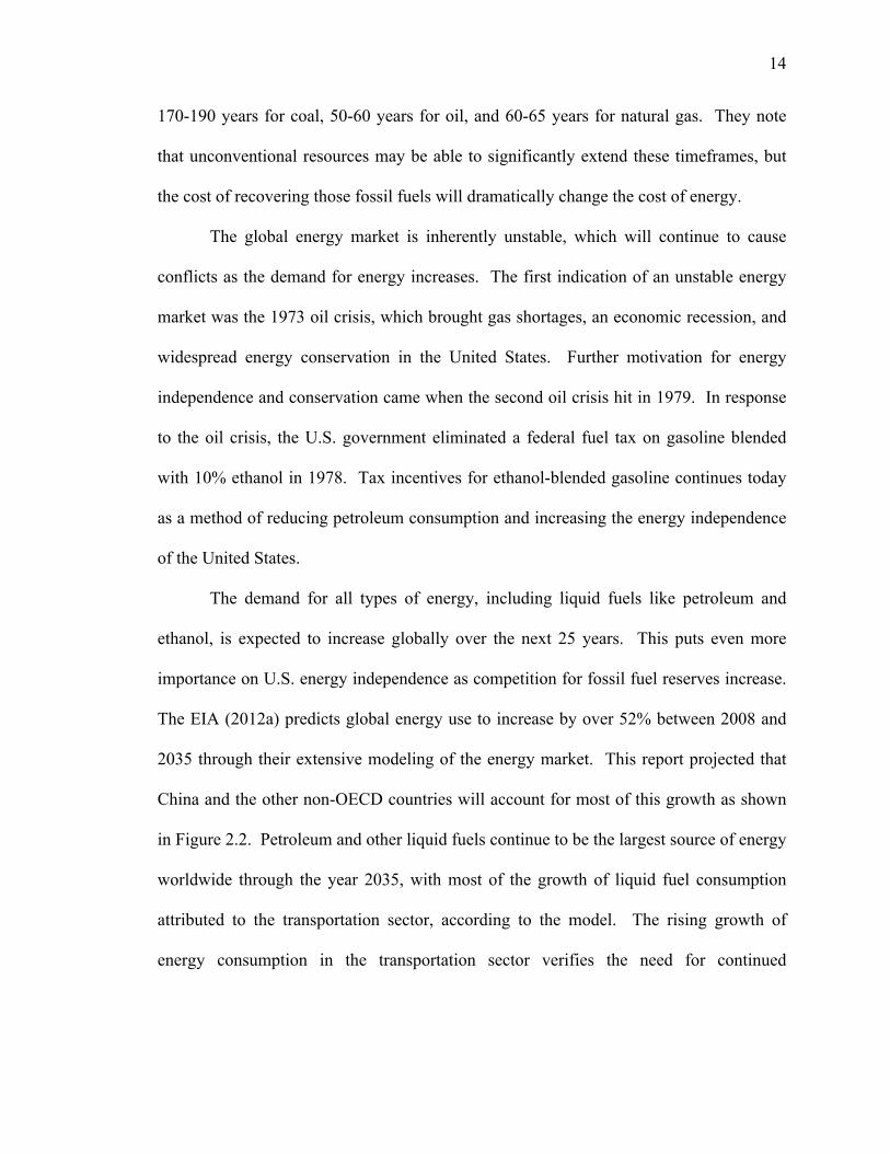
The EIA (2012a) predicts global energy use to increase by over 52% between 2008 and
2035 through their extensive modeling of the energy market. This report projected that
China and the other non-OECD countries will account for most of this growth as shown
in Figure 2.2. Petroleum and other liquid fuels continue to be the largest source of energy
worldwide through the year 2035, with most of the growth of liquid fuel consumption
attributed to the transportation sector, according to the model. The rising growth of
energy consumption in the transportation sector verifies the need for continued
15
development of affordable renewable energy sources for transportation. This will help
offset some petroleum consumption and decrease U.S. dependence on foreign oil.
Petroleum is the United States’ largest import, export, and most-consumed single
form of energy. The U.S. is highly dependent on the use of petroleum, which made up
36% of the total domestic energy use and 85% of the energy imports in 2011 (EIA
2012b). The transportation sector used the largest portion of petroleum, consuming 71%
of the petroleum, which made up 93% of the energy consumed by the transportation
sector. Only 4% of the energy used by the transportation sector came from renewable
energy sources, which includes fuel ethanol. With this type of energy distribution, it is
clear that petroleum has a major influence on America’s economy and must be
considered in all discussions of U.S. energy security.
Figure 2.2: World energy consumption in quadrillion Btu with historical data for 1990-2008 and projections for 2015-2035 (EIA 2011, 1).
World energy consumption, 1990-2035 (quadrillion Btu)

16
The development of gasoline alternatives has been motivated by the instability of
the oil industry. The price of oil is anything but stable. Predictions for the price of oil
are highly dependent on global relations, new oil discovery and refinement, as well as the
state of the global economy. The EIA (2012a) has projected the price of oil in three
future conditions, which is shown in Figure 2.3. The historical spike in oil prices as a
result of the two oil crises in the 1970’s can be seen in the first half of the 1980’s. Oil
prices rose through the 2000’s and dropped as a result of the worldwide economic
downturn in 2008. The price of oil is recovering and is expected to steadily increase for
the next 20 years in addition to inflation. The high and low oil price cases represent high
demand and low demand for oil respectively. It is clear that oil prices in the future will
be highly variable and hard to predict. This is one of the many reasons to reduce oil
consumption by use of biofuels thus reducing dependence on foreign oil and depletion of
reserves.
Average annual world oil prices in three cases, 1980-2035 (2010 dollars per barrel)
Figure 2.3: World oil prices in 2010 dollars per barrel for the EIA reference, high oil price and low oil price cases (EIA 2012a, 24).
17
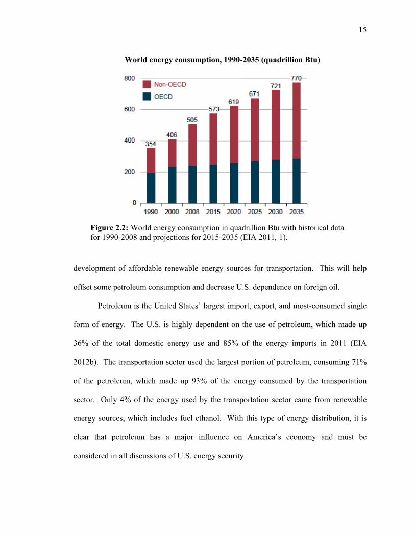
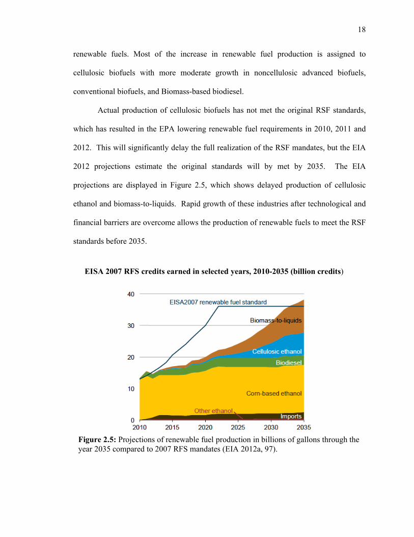
The United States has taken a strong stance supporting the production and
expanded development of renewable fuels. The Energy Policy Act of 2005 created the
Renewable Fuel Standard (RFS), which mandates the amount of renewable fuels that are
blended with transportation fuel. The policy was expanded in 2007 to create renewable
fuel standards through 2022. Much of the expanded production of renewable fuels
mandated by the RFS must reduce GHG emissions by 50% or more, which eliminates
conventional corn ethanol as a possibility. This does not indicate that corn ethanol is
being phased out but merely limits vast expansion of the industry. Corn ethanol
production is still expected to grow over the next 10 years. However, cellulosic and
advanced biofuels are anticipated to dramatically expand over this same period. The RFS
transportation biofuels mandates are illustrated in Figure 2.4. The graph shows rapid
growth of the biofuels industry, with increasing production required across all types of
RFS Mandated Consumption of Renewable Fuels, 2009-2022 (billion gallons per year)
Figure 2.4: RSF renewable fuels mandates through 2022 (EIA 2012a, 4)
18
renewable fuels. Most of the increase in renewable fuel production is assigned to
cellulosic biofuels with more moderate growth in noncellulosic advanced biofuels,
conventional biofuels, and Biomass-based biodiesel.
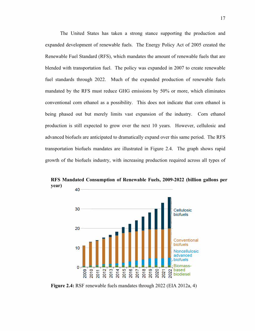
Actual production of cellulosic biofuels has not met the original RSF standards,
which has resulted in the EPA lowering renewable fuel requirements in 2010, 2011 and
2012. This will significantly delay the full realization of the RSF mandates, but the EIA
2012 projections estimate the original standards will by met by 2035. The EIA
projections are displayed in Figure 2.5, which shows delayed production of cellulosic
ethanol and biomass-to-liquids. Rapid growth of these industries after technological and
financial barriers are overcome allows the production of renewable fuels to meet the RSF
standards before 2035.
Figure 2.5: Projections of renewable fuel production in billions of gallons through the year 2035 compared to 2007 RFS mandates (EIA 2012a, 97).
EISA 2007 RFS credits earned in selected years, 2010-2035 (billion credits)

19
The motivation behind the RSF mandates is two-fold. Increasing biofuels
production reduces gasoline consumption which in turn reduces oil imports. This
improves U.S. energy independence and reduces the effects of fluctuations in global oil
prices. Domestic production of biofuels creates jobs and supports local economies, while
importing foreign oil does little to support the U.S. economy. Another desired effect of
the biofuel mandates was a more rapid reduction of GHG emissions. When biofuels are
compared to petroleum transportation fuels on a life-cycle basis, they can significantly
reduce GHG emissions.
The burning of these fossil fuels produces large quantities of carbon dioxide and
other greenhouse gases. The intergovernmental panel on climate change concludes that:
Most of the observed increase in global average temperature since the
mid-20th century is very likely due to the observed increase in
anthropogenic greenhouse gas concentrations… Recent data confirm that
consumption of fossil fuels accounts for the majority of global
anthropogenic greenhouse gas concentrations (Eidenhofer et al. 2011).
This report by the Intergovernmental Panel on Climate Change (IPCC) concludes that
human consumption of fossil fuels has led to climate change. Among other suggestions,
the IPCC recommends improving energy conservation and efficiency while developing
renewable energy sources to mitigate climate change. Not only can renewable energy
sources reduce GHG emissions, but they can also lead to economic development, greater
energy independence, and reduce negative impacts on the environment and human health
(Eidenhofer et al. 2011). Some of the effects of climate change are loss of glaciers, loss
of species, increase in severe weather, and increased flooding. Renewable energy

20
sources like solar, wind, and biofuels have the potential to replace energy produced by
fossil fuels, reduce GHG emissions, and increase U.S. energy independence while
reducing contributions to climate change.
Energy is a complex problem and will not be solved with a single solution.
Systematically reducing energy consumption and increasing the use of available
renewable resources will extend the life of fossil fuel resources, reduce the vulnerability
of the U.S. to uncertain global relations, and hopefully decrease the negative effects of
global climate change by reducing GHG emissions.
2.4 Wind Energy
Wind power is a renewable source of electricity that is available across the
country and across the globe. Power can be generated in large wind farms, distributed in
community wind projects, or produced in large offshore installations. The versatility of
wind power has lead to installations in 38 U.S. states and 75 countries worldwide
(GWEC 2012). There are currently 5 U.S. states that generate at least 10% of their
electricity from wind power, with North Dakota producing 22% of its electricity from
wind power in 2011 (Roney 2012). Turbines do not produce GHG emissions nor do
they have continuous fuel and water requirements like most forms of electricity
generation. Individual turbines use very little space and can be placed on land used for
other purposes including farmland or private businesses. Electricity production from
wind turbines is rapidly increasing. The wind market has grown significantly due to
government incentives and falling turbine prices. Wind is the fastest growing form of
renewable electricity generation and is slated to continue to grow over the next 20 years

21
and beyond. Even though the number of wind projects has vastly increased over the last
six years, electricity generation form wind only accounted for 3.3% of the U.S. electricity
demand at the end of 2011 (Wiser and Bolinger 2012). There are still many avenues for
expanded development of the wind market, but it is unlikely that wind power alone can
solve the global energy problem.
Large-scale turbines are precisely designed to extract as much energy from the
wind as possible. The growing demand for wind energy has broadened the market, which
now includes turbines for a large range of wind speeds, conditions, and power capacities.
Wind turbines convert the linear kinetic energy of the wind to rotational energy that turns
a generator, which converts this energy into electricity. Precisely designed turbine blades
are designed similar to an airplane wing in that the air has a longer distance to travel on
one side of the blade as compared to the opposite side. Wind flows over the blade and
creates lower pressure on the downside of the blade. The pressure difference causes the
blades to rotate around a central shaft or rotor. The pitch of the blades can be adjusted
with changing wind speeds to obtain the proper rotational speed. The direction the
turbine is facing can also be adjusted as the wind direction changes. A brake is also
included on the rotor to prevent damage from excessive wind speeds or allow
maintenance. These adjustments are generally performed by the control system that
receives information from an attached anemometer and wind vane to measure wind speed
and direction.
The large size of the average utility scale wind turbine means that the rotor only
completes about 6-18 revolutions per minute. The RPM is increased to around 1800
RPM by a system of gears, which is generally called the gearbox. This faster rotation
22
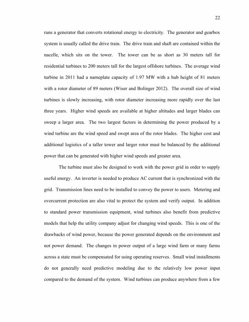
runs a generator that converts rotational energy to electricity. The generator and gearbox
system is usually called the drive train. The drive train and shaft are contained within the
nacelle, which sits on the tower. The tower can be as short as 30 meters tall for
residential turbines to 200 meters tall for the largest offshore turbines. The average wind
turbine in 2011 had a nameplate capacity of 1.97 MW with a hub height of 81 meters
with a rotor diameter of 89 meters (Wiser and Bolinger 2012). The overall size of wind
turbines is slowly increasing, with rotor diameter increasing more rapidly over the last
three years. Higher wind speeds are available at higher altitudes and larger blades can
sweep a larger area. The two largest factors in determining the power produced by a
wind turbine are the wind speed and swept area of the rotor blades. The higher cost and
additional logistics of a taller tower and larger rotor must be balanced by the additional
power that can be generated with higher wind speeds and greater area.
The turbine must also be designed to work with the power grid in order to supply
useful energy. An inverter is needed to produce AC current that is synchronized with the
grid. Transmission lines need to be installed to convey the power to users. Metering and
overcurrent protection are also vital to protect the system and verify output. In addition
to standard power transmission equipment, wind turbines also benefit from predictive
models that help the utility company adjust for changing wind speeds. This is one of the
drawbacks of wind power, because the power generated depends on the environment and
not power demand. The changes in power output of a large wind farm or many farms
across a state must be compensated for using operating reserves. Small wind installments
do not generally need predictive modeling due to the relatively low power input
compared to the demand of the system. Wind turbines can produce anywhere from a few
23
kilowatts of power for residential sized systems or over 7 MW of power for the largest
turbines available. The power ratings of turbines will be described in greater detail in the
following sections.
The U.S. wind industry is showing large capacity additions despite a struggling
economy. Over 70% of the total installed capacity was added in the past five years.
Despite a substantial drop in new wind projects in 2010 due to economic uncertainty, the
total installed wind capacity in 2011 was nearly 47 GW as compared to about 11 GW in
2006 (Wiser and Bolinger 2012). The average project price as well as the maintenance
costs of new projects continues to decline according to Wiser and Bolinger. Many wind
projects have benefited from renewables portfolio standards (RPS) in their respective
states that require a certain percentage of electricity production come from renewable
sources. State and federal incentives provide financial support, which has made wind
power more favorable to investors that want to reduce the financial risks of a new project.
The two main incentives for wind projects are the Business Energy Investment
Tax Credit (ITC) and the Renewable Electricity Production Tax Credit (PTC) (DSIRE
2012). The ITC provides a 30% tax credit on the installed cost of specific renewable
energy projects. The PTC allots $0.022 per kWh generated by certain renewable
electricity projects. Both of these credits are expiring for large-scale wind projects at the
end of 2012 and may not be extended.
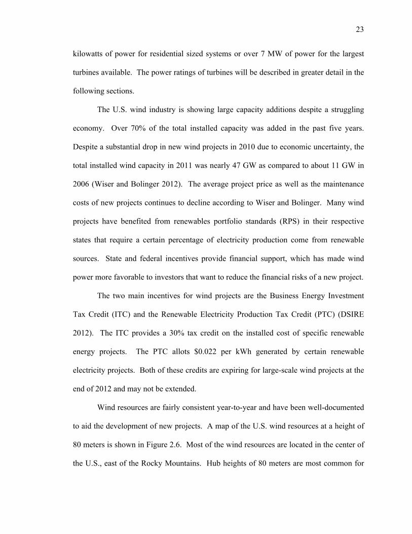
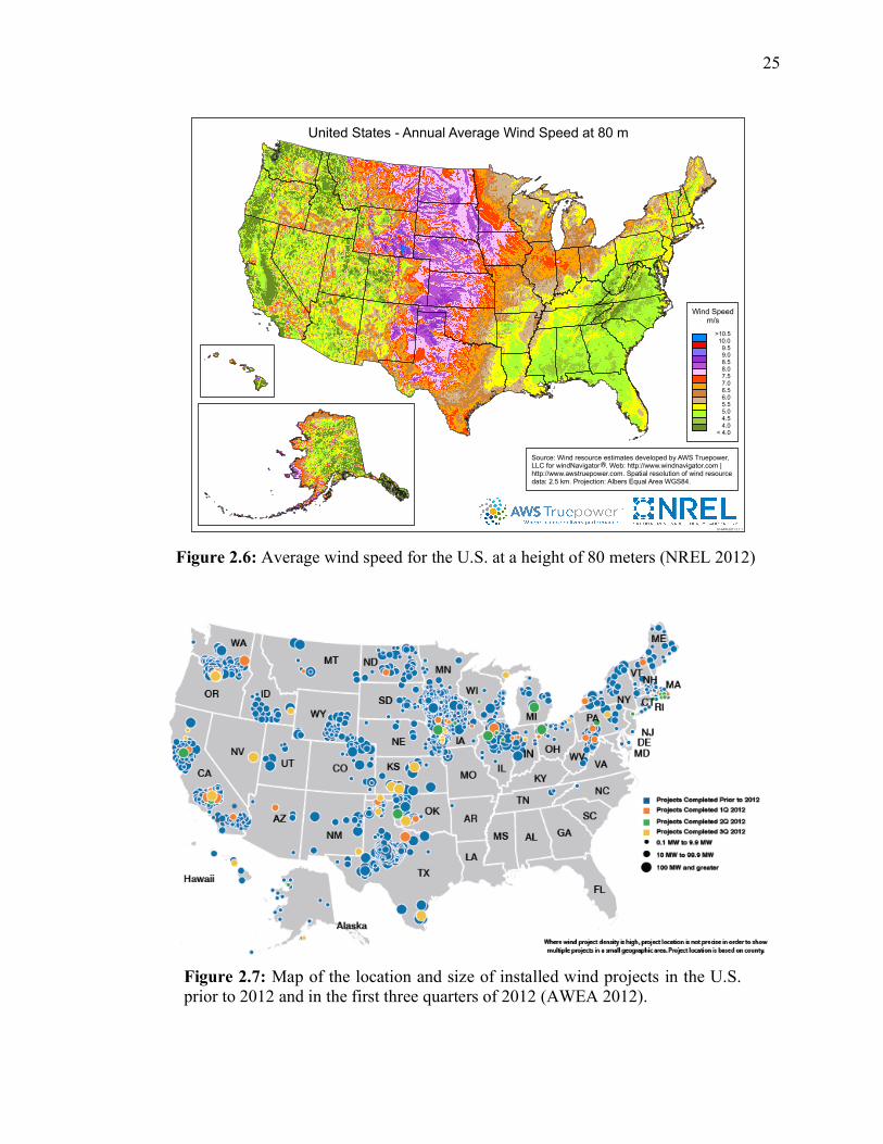
Wind resources are fairly consistent year-to-year and have been well-documented
to aid the development of new projects. A map of the U.S. wind resources at a height of
80 meters is shown in Figure 2.6. Most of the wind resources are located in the center of
the U.S., east of the Rocky Mountains. Hub heights of 80 meters are most common for

24
large and utility scale wind projects. Community wind projects have smaller turbines
with hub heights of 50 meters, while residential hub heights are around 30 meters. Much
of the installed wind capacity is located in areas with average wind speeds of 6.5 m/s or
larger, which is considered suitable for wind large-scale wind development according to
the DOE. A map of the locations and sizes of wind turbines installed in the U.S. as of the
third quarter of 2012 is shown in Figure 2.7. The locations on the map are not exact to
more clearly show the number of wind installations. Wind projects are spread across the
country, but notably there are still large areas of the country that are suitable for wind
installations that have not been utilized. This will allow expansion of the industry for
years to come.
The growth of the wind industry in the U.S. has been rapid due in part to
progressive energy standards and incentives, but the future of government support for
wind power is uncertain. Federal and state incentives have contributed to increased wind
installations, but many of these incentives have reached their distribution limits or are
expiring at the end of 2012 (DSIRE 2012). Typical incentives reimburse part of the
installed cost, guarantee the purchase price for electricity produced, or give tax credits for
equipment depreciation. In particular, turbine manufacturers are waiting to see if the
PTC will be extended beyond 2012. If this credit is not extended, industry experts
predict dramatically reduced sales in 2013. Diminishing grants, incentives and tax credits
are expected as the industry matures and moves into a more sustainable level of
government support. Even with reduced funding for projects, wind power is profitable
and will continue to grow. Growth in the U.S. may be slower than in recent years, but
projections for the future of the industry all indicate robust expansion.
25
Figure 2.6: Average wind speed for the U.S. at a height of 80 meters (NREL 2012)
Figure 2.7: Map of the location and size of installed wind projects in the U.S. prior to 2012 and in the first three quarters of 2012 (AWEA 2012).
United States - Annual Average Wind Speed at 80 m
01-APR-2011 2.1.1
Wind Speedm/s
>10.5 10.0 9.5 9.0 8.5 8.0 7.5 7.0 6.5 6.0 5.5 5.0 4.5 4.0 < 4.0
Source: Wind resource estimates developed by AWS Truepower,LLC for windNavigator . Web: http://www.windnavigator.com |http://www.awstruepower.com. Spatial resolution of wind resourcedata: 2.5 km. Projection: Albers Equal Area WGS84.
¶

26
Despite short-term uncertainty in the U.S. wind market, global wind capacity is
predicted to continue to expand through 2035. The EIA (2012a) projects that wind power
will account for 60% of the non-hydropower renewable energy generation increases from
2010 to 2035. Hydropower remains the largest source of renewable electricity generation
even with the dramatic expansion of wind capacity. Projections for the growth of wind
power and other renewable sources of electricity are shown in Figure 2.8. The world
generation of wind power was less than 400 billion kWh in 2010, but is projected to
reach over 1,500 billion kWh by 2035 (EIA 2012a). Even with this significant increase
in capacity, the EIA projections still have U.S. electricity generation from all renewable
sources accounting for only 15% of the total demand in 2035. If renewable energy
policies are extended, wind power will see increased growth over this reference case
(EIA 2012a). From this prediction, it is clear that wind will make up a substantial portion
of the worlds’ energy mix in the future.
World renewable electricity generation by source, excluding hydropower 2005-2035 (billion kWh)
Figure 2.8: World renewable electricity generation by source without hydropower with historical data from 2005 to 2010 and projections from 2010 to 2035 in billion kWh (EIA 2012a, 75).
27
There are some obstacles that make large-scale wind power slightly more
complicated. Wind turbines can obscure the landscape, produce noise, and cast shadows.
Most of these issues are most severe within a half mile of the turbine. All of these things
make it difficult to install turbines near communities and densely populated areas.
Projects may require approval by the community before planning can continue.
Fortunately, most ethanol plants are located away from towns with adequate space for a
turbine in a cornfield. Despite the few negative aspects of wind turbines, 89% of
Americans believe increasing wind power is a good idea (Swofford 2010). The negative
impacts of wind turbines should be considered during the planning stages of a project, but
widespread support for wind power should make project approval easier. Wind power
will be a substantial part of U.S. electricity generation for many years to come.
2.5 Solar Thermal Energy
The use of solar energy for heating is not a new idea, but advancing technologies
are making it possible to use solar thermal energy for large-scale applications for
numerous end uses. Solar thermal collectors work on the general premise of using solar
energy to heat a fluid, which can then be used to provide thermal energy. Low
temperature applications (below 120oC) can use non-concentrating flat plate or evacuated
tube collectors. Higher temperatures can be achieved with concentrating collectors that
use reflectors to greatly increase the temperature of the working fluid. Concentrating
collectors are generally much more expensive and require more space to process the same
amount of fluid as non-concentrating collectors. Since none of the processes in an
ethanol plant require fluid above 120oC and most of the ethanol plants are not located in
28
prime concentrating solar regions, only non-concentrating collectors will be considered
for thermal energy production at ethanol plants.
Solar thermal energy is available year round across the United States. However,
the overall efficiency of the solar collectors is greatly affected by location. Collector
efficiency decreases as the temperature difference between the working fluid and ambient
air increases. Efficiency is also negatively affected by decreasing solar insulation, which
occurs during the winter months. This means that areas of the U.S. that have large
temperature swings between summer and winter will see enormous differences in energy
obtained from a solar thermal system throughout the year. The solar installation will also
produce no energy overnight and may not produce energy on particularly overcast or cold
days. All of these factors make solar thermal systems suitable for supplemental heat as
opposed to the main source of process heat.
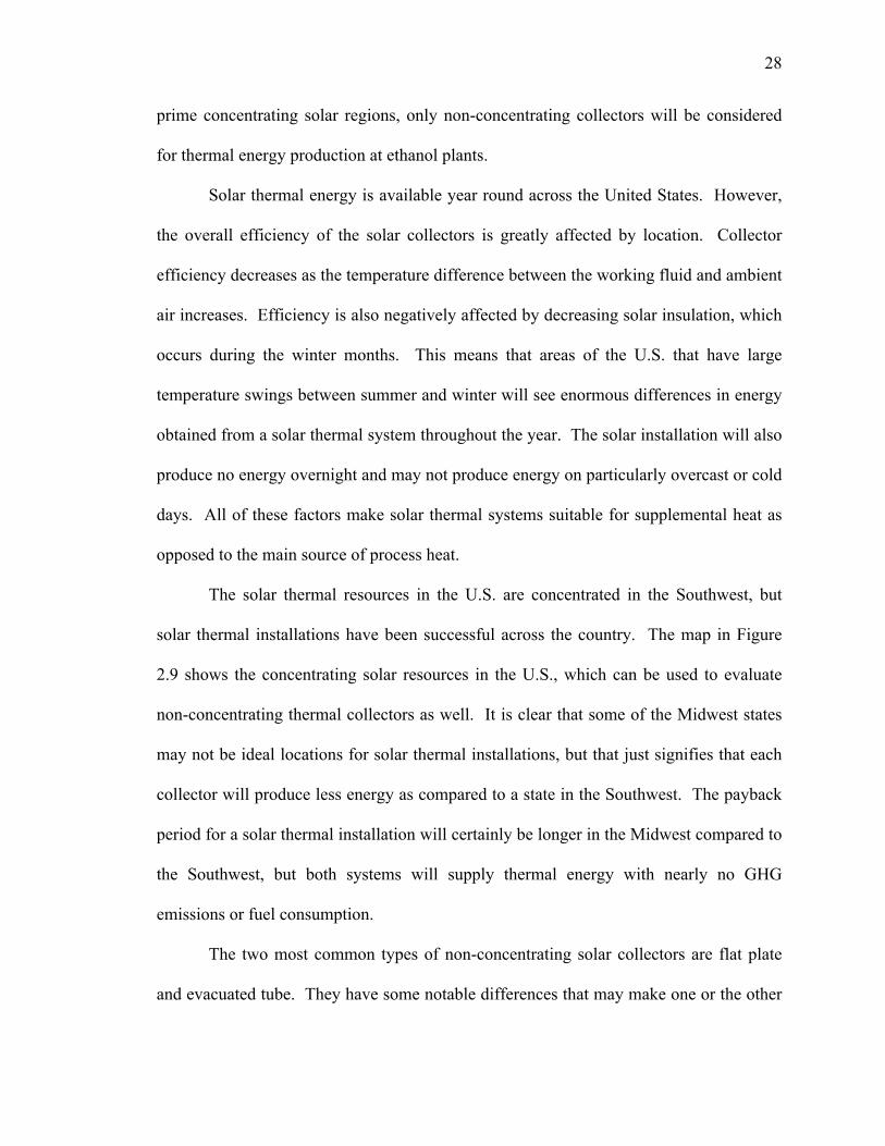
The solar thermal resources in the U.S. are concentrated in the Southwest, but
solar thermal installations have been successful across the country. The map in Figure
2.9 shows the concentrating solar resources in the U.S., which can be used to evaluate
non-concentrating thermal collectors as well. It is clear that some of the Midwest states
may not be ideal locations for solar thermal installations, but that just signifies that each
collector will produce less energy as compared to a state in the Southwest. The payback
period for a solar thermal installation will certainly be longer in the Midwest compared to
the Southwest, but both systems will supply thermal energy with nearly no GHG
emissions or fuel consumption.
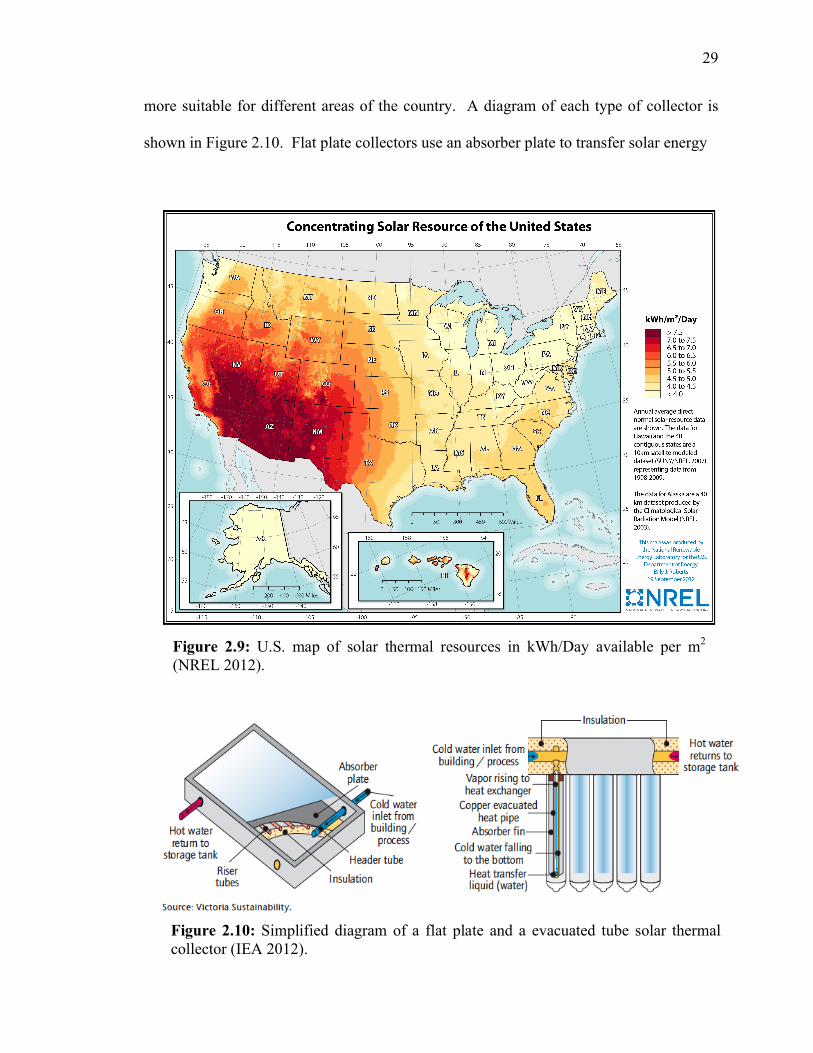
The two most common types of non-concentrating solar collectors are flat plate
and evacuated tube. They have some notable differences that may make one or the other
29
more suitable for different areas of the country. A diagram of each type of collector is
shown in Figure 2.10. Flat plate collectors use an absorber plate to transfer solar energy
Figure 2.9: U.S. map of solar thermal resources in kWh/Day available per m2 (NREL 2012).
Figure 2.10: Simplified diagram of a flat plate and a evacuated tube solar thermal collector (IEA 2012).

30
to tubes of fluid that pass through the plate. The only protection from ambient conditions
is the air gap between the absorber plate and the protective glass cover and the insulation
on the back of the panel. This makes flat plate collectors susceptible to substantial heat
loss in cold climates and may freeze if the temperature drops low enough. Evacuated
tube collectors are generally less vulnerable to freezing and heat loss because the tubes
around the working fluid are evacuated to reduce heat transfer to the ambient air. The
advantages of flat plate collectors are that they are less expensive in the U.S. and have
lower maintenance costs. Some of the tubes in an evacuated tube system will eventually
lose their vacuum, which will require time and materials to repair.
A study completed by Ayompe et al. (2011) compared the performance of a flat
plate collector and an evacuated tube collector with a closed glycol system over an entire
year in the temperate climate of Dublin, Ireland. Most studies test panels under ideal
conditions or more favorable ambient temperatures, but real-world experiments give a
better representation of the actual energy output of a collector. The overall system
performance averaged over the entire year for the flat plate was 37.9%, which was
significantly less than the 50.3% efficiency for the evacuated tube system. The collectors
themselves had efficiencies of 46.1% and 60.7% for the flat plate and evacuated tube
panels respectively. The total system efficiency was decreased by pipe heat losses, which
amounted to about 17% of the total energy collected. It is clear that even with pipe
insulation, there will be significant heat losses in solar thermal arrays. Ireland has low
solar resources, but the solar thermal arrays were able to provide hot water for the
experiments. The solar resource in Ireland is about 2.68 kWh/m2/day (Stackhouse 2012),
which is over 30% lower than any of the locations considered for this study.

31
Solar thermal systems are an effective alternative to water heating using fossil
fuels. They use very little energy to operate compared to a traditional natural gas or
electric heater with nearly 100% reduction in GHG emissions and fossil fuel use. Large-
scale water heating systems will be limited by the space available and capital required to
install the equipment. The long lifespan of the equipment and low maintenance costs
ensure low cost energy production for decades. Solar installations are generally not
plagued by as many aesthetic issues as wind turbines. They do not produce any noise,
cast large shadows, or obstruct the landscape. This makes project approval easier
because the community is not usually as concerned about the decision.
2.6 Summary
The use of wind and solar energy to offset fossil fuel consumption at ethanol
plants is conceptually viable and aligns with U.S. goals to increase production of biofuels,
decrease fossil fuel use, and reduce greenhouse gas emissions. The ethanol, wind, and
solar industries are well established and are projected to increase substantially over the
next 20 years or more. Advancing technologies and increased production are making
each of these sectors more economically viable and prime for increased development.
The future of energy is uncertain, but ethanol, wind, and solar can help America reach its
energy goals right now.

32
CHAPTER 3: MODELING TECHNIQUE AND APPROACH
3.1 Introduction to the Model
A model was created to investigate the viability of installing a wind turbine and/or
a solar thermal array at various U.S. ethanol plant locations to reduce fossil fuel use.
This model can be used in a variety of ways. The main focus was to determine if any U.S.
ethanol plants are located in areas with sufficient solar and/or wind resources to provide a
reasonable payback period and limited risks for specific renewable energy installations.
The model can also be used to evaluate any location with user-entered meteorological
and resource data. This allows the model to be used for other ethanol plant locations that
were not considered or to investigate sites for future ethanol plants. Numerous input
variables allow the model to be used for a wide range of projects and market conditions.
The following sections discuss in detail the inputs for the model and assumptions made
using current industry data and future projections.
The output data from this model can be used to evaluate a large range of projects
and future conditions. Current and projected energy prices are used to estimate yearly
cost savings and payback periods for modeled renewable energy installations. Projects
can be compared using small or large specification changes to determine optimal or worst
case system performance. Details of the output data and potential applications will be
discussed in the subsequent sections.
The basic function of the model is to use input data to estimate realistic energy
production of an installed solar array and wind turbine. This spreadsheet-based model
uses operator-entered data to estimate yearly energy production, cost savings, and
33
lifetime savings of a given system. The user enters resource data for the location, wind
turbine specifications, and solar array specifications. These values are used to find the
yearly energy production of the renewable projects. Average electricity and gas rates are
used to find payback periods and lifetime net savings of the solar and wind installations.
These results can then be analyzed to determine if the location is suitable for wind or
solar energy projects.
This model was designed to work with and expand upon the work completed by
Kumar (2009) for his Master’s thesis in which he developed a model to estimate the
energy required to produce corn ethanol at dry mill plants using only natural gas for
thermal energy. His model uses detailed inputs for the various processes required to cook
and distill ethanol to determine the required thermal energy inputs. The energy estimates
are then used to size a wind turbine and solar thermal array to replace a specified
percentage of the energy inputs. The wind and solar estimates are very rudimentary and
do not consider variations in wind and solar resources throughout the year, the use of
commercially-available equipment, or reduced output of wind and solar installations due
to low resources. Considerations for rising energy costs or the cost to install the systems
were not completely studied as well. The model developed for this research project more
accurately estimates useful energy production and payback periods for wind and solar
thermal installations. The current model can use the thermal energy requirement for a
specified ethanol plant calculated with the Kumar (2009) model and use it as an input.
Another difference between the two models is that the current model is used to
investigate solar and wind installations at 18 different ethanol plants across the country
for their actual nameplate capacity. The ranges for the input variables are also

34
investigated to determine the effect on output data and the possible span of annual cost
savings and payback periods. All of these improvements increase the accuracy and
applicability of the model.
3.2 Energy Use by Ethanol Plant
The first section of the model requires input data for the capacity of the ethanol
plant and energy usage. These values are used to determine the plant’s thermal energy
use and electricity use per year. The input field of the spreadsheet is shown in Figure 3.1.
The input cells to the model are always green and the output cells are always red to aid
understanding.
Ethanol Plant Inputs Typical Values Input
Ethanol Plant Capacity, PC (million gallons per year MGY) 1 -‐ 130 Electricity Requirement, ER
(kWh/gal-‐ethanol) 0.74 kWh/gal Heating Energy Requirement, QAE
(Btu/gal-‐ethanol) 29,000 Btu/gal Makeup Water Energy Requirement, QMW
(Btu/gal-‐ethanol) 1,365 Btu/gal
Nameplate ethanol production capacity of a given ethanol plant is the main factor
in determining energy use for the facility. The first entry on the spreadsheet is the
production capacity in million gallons per year (MGY) of anhydrous ethanol. All values
for ethanol will be assumed to be anhydrous ethanol unless otherwise noted. Capacity
Figure 3.1: The spreadsheet inputs and typical values for the ethanol plant modeling section.

35
values are published for all currently operating plants online and in many ethanol
publications (RFA 2012c). Most plants produce between 40 and 100 MGY. Equation
(3.1) estimates the total thermal energy needed for an ethanol plant.
𝑄!"#$% = 𝑃𝐶 × 𝑄!" (3.1)
The total yearly heating requirement for the plant (QTotal) in MMBtu is found by
multiplying the plant capacity (PC) in MGY by the heating rate required to produce
anhydrous ethanol (QAE) in Btu/gal-ethanol. Kumar’s (2009) ethanol production energy
model can be used to easily calculate QAE for various plant conditions by adding together
the output values of the total energy to cook (𝑄!"!""#) and the total energy to distill (𝑄!"! )
per unit anhydrous ethanol shown in Equation (3.2).
𝑄!" = 𝑄!"!""# + 𝑄!"! (3.2)
The value for QAE can also be found by using averages found from actual operational
ethanol plants. A survey of 90 ethanol plants showed that the average dry mill corn
ethanol plant used 28,859 Btu/gal-ethanol for plants using natural gas in 2008 (Mueller
2010). It is not essential that this number exactly matches a particular facility’s energy
consumption, because it is mainly used to determine the percent of total energy use that
the wind and solar installations replace.
The electricity consumption of an ethanol plant can be obtained from actual plant
operations or estimated using averages and rules of thumb. BBI International (2003)
estimates an ethanol plant’s electricity requirement at 0.8 kWh/gal-ethanol. Mueller’s
survey (2010) of 90 dry mill plants reported an average electricity usage of 0.74
kWh/gal-ethanol. Similar to the thermal energy requirement of ethanol plants, the

36
electricity requirement (ER) is used to find the percentage of electricity replaced by wind
power so precise values are not required.
The percent shift for the total natural gas heating requirement of the ethanol plant
to solar thermal energy is most likely going to be very small. Ethanol requires substantial
amounts of energy to cook and distill, primarily due to the shear volume of water and
mash that must be heated. Most plants reuse most or all of the process water to take
advantage of the residual heat remaining after the ethanol has been distilled out. This
means there will be much smaller amounts of makeup water necessary to replace boiler
water than the total water requirement of the ethanol production process. The average
fresh water requirement of a survey of 73 dry mill natural gas plants was 2.72 gallons of
water per gallon of ethanol produced (Mueller 2010). Aden (2007) reports that most of
the fresh water use in ethanol plants is makeup water for the boiler and cooling tower due
to nearly complete reuse of process water. This report also specifies that about 68% of
the makeup water goes to the cooling tower and 32% goes to the boiler with estimated
water use of 3 - 4 gallons of water per gallon of ethanol for dry mill plants (Aden 2007).
The boiler makeup water requirement in gallons of water per gallon of ethanol (MWB) is
given by Equation (3.3).
𝑀𝑊! = 𝑀𝑊!"!#$ %𝑊! (3.3)
The total makeup water requirement (MWtotal) for the plant is multiplied by the percent
of the makeup water going to the boiler (%WB). If the average value of 3 gal-water/gal-
ethanol were used for MWtotal, then the necessary boiler makeup water would be about
0.96 gal/gal-ethanol. Heating requirements for the boiler makeup water will be
significantly less than the total heating requirement of the plant. The heating requirement

37
for the boiler makeup water will be found to determine the amount of heat the solar array
would need to provided to heat the boiler makeup water from the ground water
temperature (Tgw) to the boiler input water temperature (TB). The makeup water heating
requirement (QMW) in kJ/gal-ethanol is determined by Eq. (3.4).
𝑄!" = 𝑀𝑊! × 𝑐!,! × 𝑇! − 𝑇!" × !,!!! !"!! × ! !!
!"#.! !"#,!"#$% (3.4)
Using the specific heat of water (cp,w = 4.19 kJ/kg-oC ), a boiler inlet temperature of
100oC, and a ground water temperature of 15oC, the heating requirement for the makeup
water is 1,294 kJ/gal-ethanol or 1,365 Btu/gal-ethanol. This is significantly less than the
total thermal energy of 28,859 Btu/gal-ethanol reported by the average dry mill plant in
Mueller’s survey (2010). The boiler makeup water heating requirement is less than 5%
of the total heating requirement of the plant.
Using the makeup water heating requirement significantly increases the
percentage of heating a solar thermal array can replace. Kumar (2009) did not consider
the difference between reheating recycled process water and preheating boiler makeup
water. The biggest difference between these two methods is the inlet temperature to the
panels. Recycled process water will be much warmer than makeup ground water, which
will increase the temperature of the solar array working fluid and increase heat loss from
the collectors. Using low temperature ground water increases the efficiency of the solar
array by reducing heat loss, which increases the total energy the solar array can provide.
3.3 Resource and Meteorological Inputs
This model can be used with monthly or yearly averages for solar insolation on a
tilted surface, wind speed, temperature, and daylight hours. These values are used to

38
calculate the available resources for a solar array and wind turbine. Figure 3.2 shows the
input format of the spreadsheet model for meteorological and resource values. The
averaged monthly values were obtained from a NASA sponsored web site (Stackhouse
2012) that provides measured and calculated values averaged from 22 years of data.
These values generally agree with the wind and solar resource maps shown in Figure 2.6
Location:
Resource and Meteorological Inputs
Jan Feb Mar Apr May Jun Jul Aug Sep Oct Nov Dec
Solar Insolation on a tilted surface, Gt (kWh/m2/day)
Monthly Average Air Temperature, Ta (
oC)
Monthly Average Wind Speed, Va (m/s)
Average daylight hours per day, Hday
and Figure 2.9 produced by NREL (2012), which can also be a source for yearly average
wind and solar resource values. The values from the NASA website provide greater
detail than the resource maps provided by NREL, which is important because monthly
values for solar and wind resources vary significantly from month-to-month. These two
sources of wind and solar resources provide slightly different values, which can
drastically affect model outputs. The best inputs would be from data collected near the
Figure 3.2: Spreadsheet model input field for monthly averaged resource and meteorological data.
39
plant site. To obtain values from the NASA website (Stackhouse 2012), the user enters
the latitude and longitude of the location and then selects the desired datasets. The
datasets used for the model are “Daylight Hours” (Hday), “Radiation on equator-pointed
tilted surfaces” (Gt), “Daily Temperature Range at 10m” (Ta), and “2) Gripe Power Law
used to adjust Wind Speed at 50 m to other heights” (Va). The Gripe Power Law dataset
requires a height input for the desired wind speed at a specified height above the ground.
All of the ethanol plant locations were compared using wind speeds at 80 meters, which
is the most common height for wind turbines. This model will also work for any desired
wind turbine height. The data obtained from this website (Stackhouse 2012) for each
ethanol plant location are included in Table A.1 through A.19 in Appendix A.
The radiation on a tilted surface dataset provides values for various tilt angles.
The tilt angle closest to 25o was chosen to compare the different plant locations, but any
tilt angle can be used for the user location input section. The angle between the ground
and the collector is defined as the tilt angle and is used to optimize the incident radiation
on a solar collector’s surface. Tilt angles should be adjusted for each location to give a
balance between radiation during the summer and winter. Higher tilt angles provide
more radiation in the winter and less radiation in the summer than lower tilt angles.
Higher radiation in the winter can help guard against freezing, but this will also reduce
the energy available in the summer. The NASA dataset (Stackhouse 2012) also
calculates the optimal tilt angle for each month of the year and the average optimal tilt
angle. This information could be used to optimize designs for a solar thermal array.
Monthly resource data for solar installations is much more useful than yearly
values because the range of solar insulation throughout the year can vary widely from

40
summer to winter. This is especially true in northern states when the temperature and
solar insulation drops during the winter. During the winter, solar energy is reduced, heat
loss of the solar array increases, and daylight hours are shortened which all leads to
dramatic reductions in the available energy from the solar array. Preliminary evaluations
of a proposed solar thermal array must take into account the large variation in available
solar energy throughout the year and how this will be managed by the planned system.
The large variations in solar energy, particularly in Midwestern states where most of the
ethanol plants are located, is another reason to use the solar installations to preheat
process water or makeup water instead of producing steam or high temperature water.
The lower temperatures of makeup water reduce heat loss to the environment in colder
climates. This will also aid integration into the existing system, because the solar array
can be connected before the process to eliminate the need for major changes in plant
operation. The model can use either monthly averages or a yearly average for solar
resources, but monthly data will give a more complete picture of available thermal energy.
Wind resources also vary throughout the year, but do not have as great an effect
on plant operations. Most wind projects are grid connected, which eliminates negative
effects on process operation of changing electricity generation throughout the day and
year. It is still beneficial to calculate the changes in wind energy throughout the year to
predict variations in energy and cost savings. Yearly or monthly average wind resources
may be used with this model; however, monthly values show the range of available
energy throughout the year more accurately.

41
3.4 Calculating Wind Power Generated
This model can be used employing two different methods to calculate the annual
electricity generation of a reference wind turbine. Users can enter monthly wind resource
data or an average yearly wind speed value in m/s. These values can either be actual
wind averages for the location considered or the design values for the wind turbine. The
type of data will determine how the operator uses the model. The individual input data
required for each method is listed under the specific title. Monthly wind resource data is
entered into the spreadsheet in the appropriate green cells shown in Figure 3.2. The input
fields of the spreadsheet for specific wind turbine information are displayed in Figure 3.3.
Typical values are given for input values to aid the user in obtaining an accurate model of
energy generation. Some of the input labels indicate that there are two possible variables
that can be entered into that cell. This allows the model to perform different calculations
depending on user needs. Notes are also included in the spreadsheet to help direct the
user on the appropriate use of the model.
Wind Inputs Typical Values Input
Design Wind Speed for Turbine, Vd (m/s) 8-‐15 m/s Installed Cost of Wind Turbine, ICwt ($/kW) $2,000/kW
Diameter of Turbine Blade, DR (m) 50-‐90m Monthly Wind Data
Power Coefficient, Cpa or Cpd Max: 0.59 Capacity Factor, 1 or Cfa 1 or 0.2-‐0.55
Yearly Wind Data Yearly Average Wind Speed, Va or Vd 6.5-‐15
Power Coefficient, Cpa or Cpd Max: 0.59 Capacity Factor, 1 or Cfa 1 or 0.2-‐0.55
Figure 3.3: Illustration of the wind inputs for the spreadsheet model

42
The main difference between the two types of calculations is whether the inputs
are the design parameters of the wind turbine or the actual conditions at the turbine site.
When a user enters a design wind speed (Vd) for the turbine, then a design power
coefficient (Cpd) and an actual coefficient of power (Cpa) should be entered. If the user
enters actual average wind resource values (Va), then a realistic average power coefficient
(Cpa) can be entered and the capacity factor should be set to 1.0 or something near one.
Both methods are verified for their accuracy in predicting actual electricity generation.
The actual power delivered by the wind turbine will be substantially less that the
total energy contained in the wind that flows past. The power output (Pw) of the wind
turbine is calculated using the density of air (ρa), the particular turbine coefficient of
power (CP), the swept area of the rotor blades (As), and the wind speed (Vw), as shown in
Equation (3.5).
𝑃! = 12 𝜌! 𝐶! 𝐴! 𝑉!
! (3.5)
The density of air is generally assumed to be 1.23 kg/m3 for this model. Determining the
other values is discussed in detail subsequently.
The coefficient of power is unique to every turbine and will vary as the wind
speed varies. This is why a turbine should be selected for a design wind speed that
corresponds to wind speeds at the desired turbine location. Equation (3.6) defines the
coefficient of power.
𝐶! = 𝑃𝑜𝑤𝑒𝑟 𝑔𝑒𝑛𝑒𝑟𝑎𝑡𝑒𝑑𝑊𝑖𝑛𝑑 𝑆𝑡𝑟𝑒𝑎𝑚 𝑃𝑜𝑤𝑒𝑟 (3.6)
If the coefficient of power were one, the turbine would reduce the air speed of all the
wind that crossed the swept area of the blades to zero. This is not theoretically possible,

43
and Albert Betz determined the maximum theoretical value of the coefficient of power
was 59.3%, which is known as the Betz limit (Ragheb 2011). This means that at least
40.7% of the energy contained in the wind continues past the turbine. In general, real
turbines have average coefficients of power lower than this theoretical value. Some
turbine manufactures will publish coefficient of power information for a specific design
wind speed, but average operational values will most certainly be lower than any design
numbers. This is because the stated value is for a specific design wind speed when the
turbine is most efficient.
This design wind speed results in the optimal tip speed ratio (TSR). The TSR is
the ratio of the rotor tip speed to the free stream wind speed. Deviations from the optimal
TSR reduce the coefficient of power. Typical values for coefficients of power for
changing tip speed ratios are shown Figure 3.4. As seen in the Figure 3.4, the power
coefficient peaks at an optimal TSR and is significantly lower at values far from this
value. Typical values for the coefficient of power for commercial turbines are about 0.40
(Regheb 2011). Advanced designs and reduced losses have allowed large-scale turbines
to achieve higher power coefficients for optimal wind speeds. Figure 3.5 shows the
Figure 3.4: Power coefficient as a function of tip speed ratio for a two-bladed wind turbine rotor (Regheb 2011, 33).

44
power curve of a 2.0 MW turbine calculated by the turbine manufacturer ENERCON
(2010). The maximum coefficient of power is 0.5 for this turbine. The graph also shows
how the power produced by the turbine rapidly increases as the wind speed increases
until it reaches its design power production. Once the wind speed increases above the
design speed, the pitch of the blades adjusts to control the speed of the rotors. This slows
the rotors down to maintain the desired power output. Maintaining the desired power
output quickly reduces the power coefficient because more wind energy is flowing past
the turbine without being collected. The coefficient of power is relatively stable for wind
speeds near the design speed. This makes deciding on a capacity factor to use for
calculations much easier. If the speed used for calculations is close to the design speed,
but not larger, then the design power coefficient can be used with only small errors.
Design wind speeds should always be larger than average wind speeds to take advantage
of the additional energy available as the wind speed increases. From Eq. (3.5) it is clear
that small increases in wind speed will lead to large increases in power, because the wind
Figure 3.5: Calculated power curve and power coefficient for a 2MW wind turbine as a function of wind speed at hub height from the product brochure (ENERCON 2010).

45
speed is cubed. It is tempting to increase the design wind speed to maximize power
production, but this will also decrease the coefficient of power at lower wind speeds.
Care must be taken to install a turbine that is designed to work with the wind resources
available at that particular site. A realistic coefficient of power to use to model the power
produced by a new large-scale turbine would be in the range 0.40 to 0.50. Using the
maximum value of 0.593 would overestimate power production.
The swept area in m2 is found using the rotor diameter (DR) in meters, as shown is
Equation (3.7).
𝐴! = 𝜋 𝐷!!
4 (3.7)
The average wind speed for a particular location can be found from multiple
sources. This model uses monthly data obtained from the Surface Meteorology and Solar
Energy (SSE) website (Stackhouse 2012) sponsored by NASA using the latitude and
longitude of selected ethanol plant locations. The wind speed data is calculated mainly
using 50m airport data with some adjustments based on topography and known issues
with certain regions. They report about 20-25% uncertainty for the mean monthly wind
speed values due to specific location conditions. A yearly average wind speed can be
obtained from Figure 2.6 or the individual state maps provided online by NREL (2012).
In general, wind speeds will be lower in the summer and higher in the winter, which
makes monthly averages more useful in predicting the variation of power generation
throughout the year. If monthly wind speeds are entered into the model, a graph showing
the useful electricity production each month is generated. This allows users to quickly
see how the energy output of the turbine will vary throughout the year.

46
The yearly electricity production of a wind turbine can be calculated using two
different methods. The first method uses monthly average wind speeds, a realistic
coefficient of power, and a capacity factor of one. The model assumes the average wind
speed will be below the turbine design levels, so the actual capacity factor will be far
below unity. An actual capacity factor is calculated later in the model. This first method
is used to compare the wind resources at the various ethanol plant locations. The user
can also perform these calculations by entering monthly wind speed data into the
spreadsheet as illustrated in Figure 3.2. The second method uses only one average wind
speed for the entire year. This method can be used in two different ways. The first way
is similar to the monthly data entry in that a realistic wind speed is used with a realistic
coefficient of power and a capacity factor of unity. The second way to use the yearly
wind speed method is to pick a design wind speed for a turbine with the design
coefficient of power and a realistic capacity factor (Cf). The yearly electricity production
of the modeled wind turbine (Ew) is calculated using Equation (3.8).
𝐸! = 𝑃! 𝐶! 𝐻! (3.8)
Yearly operating hours (Hy) in hours/year are assumed to be 8,760 h/yr for all simulations.
The capacity factor is mainly used for design wind speeds and is defined by Equation
(3.9).
𝐶! = 𝐴𝑐𝑡𝑢𝑎𝑙 𝑌𝑒𝑎𝑟𝑙𝑦 𝐸𝑛𝑒𝑟𝑔𝑦 𝐺𝑒𝑛𝑒𝑟𝑎𝑡𝑖𝑜𝑛
𝑌𝑒𝑎𝑟𝑙𝑦 𝐸𝑛𝑒𝑟𝑔𝑦 𝐺𝑒𝑛𝑒𝑟𝑎𝑡𝑖𝑜𝑛 𝑎𝑡 𝑀𝑎𝑥𝑖𝑚𝑢𝑚 𝐶𝑎𝑝𝑎𝑐𝑖𝑡𝑦 (3.9)
The actual capacity factor of an individual wind turbine depends on numerous aspects of
its operation, but average values are readily available. Data from 50 wind projects built
in 2010 (Wiser and Bolinger 2012) with a total installed capacity of 4,989 MW showed
that capacity factors ranged from 18% to 53% in 2011. This same report showed that the

47
weighted average of the capacity factors for 305 projects totaling 32.8 GW installed from
2004-2010 was about 34% for 2011 electricity generation data. An NREL technical
report (Tegen 2012) uses 38% capacity factor for their reference case for a 1.5 MW land-
based wind turbine. Capacity factors will be higher for projects with higher and more
consistent wind speeds and lower for areas with lower wind speeds, less consistent wind,
and areas that require curtailment of wind power to adjust for power demand. Capacity
factors will generally fall between 20% and 50% and should be adjusted to project
conditions.
The ideal energy and power generated by the turbine is calculated to determine
the actual power factor and design capacity of the proposed system. The power capacity
(PC) of the system is determined using Equation (3.10).
𝑃! = 12 𝐶!" 𝜌! 𝐴! 𝑉!
! (3.10)
This provides the nameplate capacity of the wind turbine. This capacity can be used to
estimate the installation price of the wind turbine or determine maximum power
production. Design wind speed (Vd) is used along with the turbine design coefficient of
power (Cpd) to determine the maximum amount of power that can be produced by this
turbine. Design wind speeds are generally in the 8-13 m/s range depending on location
and height. Larger design wind speeds increase the maximum power the turbine can
produce, but most often lower capacity factors. Lower design wind speeds limit the
power production, but generally increase the capacity factor because the wind speed is
close to the design wind speed more often. Equation (3.11) gives the theoretical
electricity production (Ewt) of the wind turbine if it operated at ideal conditions 24 hours
per day for the entire year.

48
𝐸!" = 𝑃! 𝐻! (3.11)
The wind turbine capacity factor (Cfa) for simulations using actual wind speeds instead of
design wind speeds is evaluated employing Equation (3.12).
𝐶!" = 𝐸!𝐸!"
(3.12)
Calculation of the actual capacity factor for the proposed wind turbine aids the user in
verifying that the values used are consistent with industry standards. If the calculated
value for the actual capacity factor is below 19% or above 53% then the proposed wind
turbine is outside the known range of over 50 installed wind projects in 2011 (Wiser and
Bolinger 2012).
The installed cost of a wind turbine (ICwt) is based on the nameplate power
capacity of the turbine. Average turbine prices fell from just under $1,400/kW in Jan
2011 to just over $1,200/kW in Jan 2012 (Wiser and Bolinger 2012). The turbine cost is
only part of the total installed cost for the turbine. The allocation of total installed costs
is show in Figure 3.6. Turbine costs account for about 68% of the installed cost of a wind
Figure 3.6: Average installed costs of land based wind turbine (Tegen et al. 2012)

49
project according to Tegen et al. (2012). Their report models the costs of wind energy in
2010, in which they use $2,155/kW as the installed cost of a 1.5MW turbine. Wiser and
Bolinger (2012) report an average capacity weighted installed cost of $2,100/kW in 2011,
and preliminary values for installed costs for 2012 projects may be well under $2,000/kW.
The average installed costs of 584 wind projects constructed between 1982 and 2012 are
shown in Figure 3.7 (Wiser and Bolinger 2012).
Installed costs peaked in 2009 and 2010 and fell in 2011 and 2012. Even though the
average installed cost is dropping, the range for total installed costs is still rather large.
The most expensive project surveyed in 2011 was about $4,500/kW while the least
expensive project was $1,500/kW, though the vast majority of the wind projects were
between $1,500 and $3,100/kW. For a 1.5 MW turbine this would result in a difference
in installed costs of $2.4 million, which is more than the cost of the cost of the
Figure 3.7: Installed project cost in 2011 $/kW for 584 projects installed between 1982 and 2012. The blue line shows weighted averages for project cost according to project size (Wiser and Bolinger 2012).

50
$1,500/kW project. It is likely that the more expensive projects have more difficult
installations and longer planning periods, which should not be an issue for ethanol plants.
Ethanol plants are typically located away from densely populated areas with abundant
land for a wind turbine. Another factor to consider in determining installed cost is the
size of the project. Wind turbines benefit from economies of scale, which means larger
projects generally have a lower installed cost on a $/kW basis. A comparison of 275
projects between 2009 and 2011 show an average installed cost of nearly $2,500/kW for
turbines greater than 0.1 MW and less than 1 MW, about $2,250 for turbines 1 MW to
less than 1.75 MW, and about $2,100 for turbines from 1.75 MW to less than 3.25 MW
(Wiser and Bolinger 2012). Due to decreasing price trends, this model will use an
average installed cost of $1,800/kW to compare wind installations at ethanol plant
locations. Simulations of varied installed costs will also be completed to account for
possible price ranges.
The outputs for the wind energy calculations are shown in Figure 3.8. All of the
wind outputs previously discussed are included, as well as the useful wind energy (EBtu)
in MMBtu/yr and the electricity generation percent of total. The useful wind energy is
Wind Outputs Design Turbine Power, Pd (MW)
Theoretical Electricity Generation, Ewt (kWh/yr) Electricity Generation, Ew (kWh/yr) Useful Wind Energy, EBtu (MMBtu/yr) Wind Turbine Capacity Factor, Cfa
Percent Shift Electricity to Wind, %Sw
Figure 3.8: Spreadsheet model outputs for wind calculations

51
calculated by dividing the electricity generation value by the general conversion factor of
293.1 !"!!!"#$
. This allows comparisons across energy types. Equation (3.13) calculates
the percent shift from traditional electricity to electricity generated by wind power (%Sw).
%𝑆! = 𝐸!
𝑃𝐶 × 𝐸𝑅 (3.13)
Percent shift is another factor that aids in verifying appropriate project input values and
relative project size. If the percent shift from conventional wind energy is very low then
the ethanol plant will not see a large reduction in energy costs, but will also have a
manageable implementation cost relative to annual profits. If the percent shift is very
large then the company will see dramatic reductions in annual electricity costs, but will
most likely need extensive financing and project backing.
3.5 Calculating the Solar Energy Collected
The solar energy collected by a proposed solar thermal array can be calculated
from monthly or yearly solar resource data. This model can estimate the thermal energy
collected by both evacuated tube and flat plate collectors with adjustments to panel
parameters. Just as with the wind resource data, average monthly solar insulation values
in kWh/m2/day are entered into the spreadsheet using the field shown in Figure 3.2.
Monthly resource data will more accurately show the available thermal energy available
throughout the year. The input field for solar data is shown in Figure 3.9. The total area
of each collector (Ac) is the gross area of each of the collectors in the solar array. The
aperture area of each collector (Aa) is the area of the collector that can absorb sunlight to
transfer thermal energy to the working fluid. For flat plate collectors, the aperture area
will be between about 85-95% of the gross area of the collector. Evacuated tube

52
collectors have slightly more variation, so the aperture area can be anywhere between 60-
85% of the gross collector area. The aperture area is not essential to the operation of the
model. It is used to calculate the efficiency of the collectors based on aperture area in
addition to gross collector area. Typical residential panels are usually between 2 and 4
square meters and are readily available. Large industrial panels can have gross areas up
to 10 m2.
The installed cost per square meter (ICsc) of the solar collectors will mainly
depend on the type of collector and the size of installation. Installed costs can be hard to
estimate, because they include costs for the design, permits, piping, panels, pumps,
insulation, a heat exchanger, storage tank and installation. Larger systems will have a
smaller cost per square meter due to economies of scale. The installation costs of large
Solar Inputs
Typical Values Input
Total Area of Each Collector, Ac (m2) 1-‐10 Aperture Area of Each Collector, Aa (m2) 60-‐95% AC
Number of Panels, Np 3 -‐ 5000 Price per Square Meter, ICsc ($/total m2) 200 – 600
FR(τα) 0.5 -‐ 0.9 FRUL (W/m2-‐oC) 0.7 -‐ 15
Average Input Temperature of Working Fluid, Ti (oC) 15 -‐100
Load Factor, Lf ≤ 1 Yearly Solar Data
Yearly Average Insulation, Gt (kWh/day/m2) 2.0 -‐ 9.0 Yearly Average Air Temperature, Ta (oC) 5.0 -‐ 20
Load Factor, Lf ≤ 1
Figure 3.9: Illustration of the solar inputs for the spreadsheet model

53
projects make up a smaller percentage of the total installed cost. RETScreen
International (2005) reports typical panel prices for flat plate collectors in the range of
$180-$310/m2 and evacuated tube collectors in the range of $900-$1,100/m2. The lower
price range is for large systems while the higher price range is for small systems. The
price range for flat plate collectors agrees with prices reported by EIA (2012) for a 2009
survey of U.S. solar thermal collector manufacturers, which reported average prices for
flat plate collectors at a rate of $19.43/ft2 and evacuated tube collectors at a rate of
$25.88/ft2. These prices are equivalent to $209/m2 for flat plate collectors and $279/m2
for evacuated tube collectors. The RETScreen numbers may also include evacuated tube
collectors with concentrators, which would dramatically increase the average price and
account for the large disparity between manufacturer and RETScreen values. Installed
costs are more difficult to estimate due to the large range of project specifications and
locations. The IEA (2012) reports that installation costs for small-scale solar hot water
systems can be up to 50% of the total cost, and large-scale systems generally have lower
installation costs compared to the equipment costs. Model inputs for total installed costs
for flat plate and evacuated tube arrays are estimated to be in the range $314-$418/m2 and
$419-$558/m2 for each type of panel respectively. These values are between 1.5 and 2
times the 2009 panel prices reported by U.S. manufacturers from the EIA website (2012).
Users can adjust these values to the specific project considered.
There are two collector performance variables that determine the amount of solar
insolation the collector absorbs and the heat lost to the environment. The variable FR(τα)
determines the percentage of solar energy absorbed, and the variable FRUL determines the
heat lost to the environment due to the temperature difference between the ambient air

54
(Ta) and the input fluid temperature (Ti). The total useful solar energy (Qu) in MJ/yr
transferred to the working fluid is calculated using Equation (3.14).
𝑄! = 𝐿!𝐴! 𝑁! 𝐹! 𝜏𝛼 𝐺! − 𝐹!𝑈! 𝑇! − 𝑇! × (𝐻!"# − 2) × !,!"" !! !!"#
× 𝑁! (3.14)
Flat plate collectors have FR(τα) values between 0.6 and 0.8, while evacuated tube
collectors have values typically between 0.5 and 0.6 based on gross collector area
(RETScreen 2005). This means that flat plate collectors will capture more solar energy
than evacuated tube collectors due to a less reflective surface. Values of FRUL for flat
plate collectors range from 3.5 to 6 W/m2-oC and range from 0.7 to 3 W/m2-oC for
evacuated tube collectors based on gross collector area (RETScreen 2005). Flat plate
collectors will lose significantly more energy due to temperature differences between
fluid temperature and ambient air temperature. Specific values of FR(τα) and FRUL may
be available from collector manufactures, but can also be found through the RETScreen
database (2012) of collector efficiency values. Average values for these performance
variables were used to compare the performance of flat plate and evacuated tube
collectors at various ethanol plant locations. The variables used to model flat plate
collectors were 0.72 and 4.5 W/m2-oC, and the variables used for evacuated tube
collectors were 0.59 and 1.5 W/m2-oC. Panels with higher values for FR(τα) and lower
values for FRUL are usually more expensive because they have a higher efficiency. The
model can simulate adjustments in price and performance variables to weigh the benefits
and disadvantages of increased performance with increased cost.
The total useful energy available for water heating is reduced by a user defined
load factor (Lf). The load factor can be less than or equal to 1.0 depending on anticipated
heat losses and reduced capacity. This value accounts for additional heat loss from
55
piping or storage tanks as well as reduced operation time due to excessively cold
temperatures or low solar energy days. Solar collector arrays will only operate when the
collectors are receiving sufficient energy from the sun. This means that there will always
be some solar energy that is wasted, because the energy received is too low to warrant
operating the system. Flat plate collectors will have a lower load factor than evacuated
tube collectors because they cannot utilize as much solar energy during the morning and
evening hours when the incidence angle is not optimal. Flat plate collectors lose more
heat due to extreme temperatures as well, which may not be accounted for if the user
enters yearly averages for the solar insulation and ambient temperature. The load factor
can also be adjusted to simulate non-ideal solar conditions or reach a desired solar
collector efficiency.
The solar insolation incident on the tilted surface of the collector (Gt) in
kWh/m2/day is the total solar energy that hits the collector. Monthly values for Gt are
entered in the spreadsheet field shown in Figure 3.2, while a yearly average value can be
entered in the field shown in Figure 3.9. The user only needs to use one of these methods
to model the proposed solar array.
The heat loss coefficient (UL) in W/m2-oC is converted to J/m2-oC-day by
multiplying by the number of hours the collector is in operation per day and the number
of seconds per hour. For monthly solar data this value is the number of sunlight hours
per day (Hday) minus two. Subtracting two from the sunlight hours accounts for the fact
that early morning and evening solar energy is too weak to operate solar arrays. The
collectors will only lose heat when the system is operating. If the user enters a yearly
value for the solar resource, Hday is assumed to be 12.

56
Total useful solar energy per year shown in Eq. (3.14) is multiplied by the number
of days (Nd) the array operates to find J/year. For monthly input data a separate value for
useful solar energy is calculated for each month by using the average number of days in a
month, 30.417 days/month. Then the monthly values are added together to give the
yearly useful energy. Yearly input data uses 365 days per year to calculate the total
useful energy. The useful solar energy per month is calculated for monthly user input
data and each of the 18 ethanol plant locations on their respective worksheets of the
model. These values are used to generate a graph each time the user runs a simulation
that shows the monthly variation in useful energy output of the solar thermal array. The
relative differences between solar energy throughout the year can help the user predict
changing thermal energy throughout the year. It can also be used to help size the array to
ensure peak summer output will not be too large.
The performances of solar thermal collectors are often compared on the basis of
efficiency. There is some debate on the best way to measure efficiency, so this model
calculates the efficiency of the total solar array and modeled panel based on gross
collector area and aperture area. The efficiency measured by aperture area will always be
larger than the efficiency measured by gross collector area, but evacuated tubes usually
benefit more from aperture efficiencies. This is because a lower percentage of their total
area can collect solar energy. Equation (3.16) determines the total solar energy incident
on the tilted surface of a collector array. Equation (3.17) gives the total energy incident
on the aperture area of the solar array.
𝑄! = 𝐴! 𝑁! 𝐺!" × 3,600 𝑠ℎ ×
365 𝑑𝑎𝑦𝑠𝑦𝑒𝑎𝑟 (3.16)

57
𝑄! = 𝐴! 𝑁! 𝐺!" × 3,600 𝑠ℎ ×
365 𝑑𝑎𝑦𝑠𝑦𝑒𝑎𝑟 (3.17)
Both these calculations use the yearly averages for solar insulation on a tilted surface
(Gta) in kWh/m2/day. These values are then used in Eq. (3.18) and Eq. (3.19) to find the
total efficiency of the solar array for gross area (ηc) and aperture area (ηa) respectively.
𝜂! = 𝑄!𝑄! (3.18)
𝜂! = 𝑄!𝑄! (3.19)
These efficiencies are then divided by the load factor to find the average efficiency of the
panels in the array based on gross area (ηcp) and aperture area (ηap) shown in Equation
(3.20) and Equation (3.21).
𝜂!" = 𝜂!𝐿! (3.20)
𝜂!" = 𝜂!𝐿! (3.21)
Values for panel efficiency are more readily available than the performance variables
FR(τα) and FRUL, so these calculated efficiencies could be compared to published,
calculated, or measured efficiencies to verify and adjust the performance variables. A
large online catalogue of test results for various flat plate and evacuated tube collectors is
available from the Swiss institute SPF (2012) to compare the efficiency calculated by the
model to test results. The catalogue also gives panel dimensions, aperture area, and panel
weight, which could aid in obtaining model inputs or preliminary designs for a solar array.
SPF (2012) tested each of these panels and reports values for ηo, a1 (W/m2K), and a2
(W/m2K2) based on panel aperture area. The panel efficiency using SPF (2012) data
(ηspf) is found using Eq. (3.22) and Eq. (3.23).

58
𝜂!"# = 𝜂! − 𝑎! 𝑇!∗ − 𝑎! 𝐺 𝑇!∗! 3.22
𝑇!∗ =(𝑇! − 𝑇!)
𝐺 (3.23)
The mean temperature of the working fluid (Tm) should be larger than the average inlet
temp (Ti) set by the user. The irradiation G (W/m2) can be found using Eq. (3.24) and
available solar resource data.
𝐺 = 𝐺!" × 1,000!
!"
𝐻!"# (3.24)
This method was used to verify the panel parameters used. The average values for ηo, a1
(W/m2K), and a2 (W/m2K2) from SPF test data are shown in Table 3.1, which are
averages found by IEA’s Solar Heating and Cooling Programme (IEA SHC) conference
proceedings (2004). The values were verified by comparing current values on the SPF
website (2012) and the averages still agree with current values on the SPF site. Using
these values, the collector efficiency was calculated for a flat plate collector with values
for FR(τα) of 0.72 and FRUL of 4.5 and an evacuated tube collector with values for FR(τα)
of 0.59 and FRUL of 1.5. The flat plate collector aperture area was assumed to be 95% of
the gross area and the evacuated tube aperture area was assumed to be 80% of the gross
collector area. Both the tested plate efficiencies (ηspf) and the calculated model
Average Efficiency Values for Solar Thermal Collectors
Flat Plate Evacuated Tube
ηo 0.79 0.76 a1 3.2 1.2 a2 0.015 0.008
Table 3.1: Average values from SPF test data for the efficiency coefficients of flat plate and evacuated tube solar collectors (IEA SHC 2004).

59
efficiencies (ηap) were the same when Tm was set to about 10oC above Ti. This verifies
that the model gives accurate estimates of panel efficiency compared to measured
efficiencies of panels in the commercial market.
Model outputs for the solar calculations are shown in Figure 3.10. The total
useful energy per year in MMBtu (Qut) is calculated by dividing the useful energy by the
standard conversion factor 1055 J/MMBtu. Equation (3.24) calculates the percent shift
from natural gas heating to solar heating (%Ss), and Equation (3.25) calculates the
percent shift from natural gas heating to solar thermal heating of the boiler makeup water
(%SMW).
%𝑆! =𝑄!𝑄!"!#$
(3.24)
%𝑆!" =𝑄!
𝑃𝐶 × 𝑄!" (3.25)
Solar Outputs Solar Energy Received on Surface of Array, Qc (MJ/yr)
Solar Energy Received on Aperture Surface of Array, Qa (MJ/yr) Useful Solar Thermal Energy, Qu (MJ/yr) Useful Solar Energy, Qut (MMBtu/yr) Solar Array Efficiency, ηc (Gross Area)
Solar Array Efficiency, ηa (Aperture Area) Solar Panel Efficiency, ηcp (Gross Area)
Solar Panel Efficiency, ηap (Aperture Area) Percent Shift From Natural Gas to Solar, %Ss
Percent Shift From Natural Gas to Solar (makeup water), %SMW
Figure 3.10: Solar outputs of the model

60
3.6 Project Costs and Savings
The main concern for any business owner is the ability to make a profit so the
business can continue to operate. Implementation costs and payback periods usually
trump the good press a company might receive for installing a renewable energy project.
This is especially true of ethanol plants that are currently producing environmentally-
friendly fuel to reduce oil consumption. Therefore this model focuses on estimating
realistic cost savings and payback periods for wind and solar installations. Some of the
logistical issues that may arise when planning or installing both of these projects are
discussed below, followed by the financial calculations of the model.
Wind and solar energy production can vary dramatically throughout the year. It
will be important to be certain the maximum output of the system will not be too large.
Since wind energy and plant energy usage varies throughout the day and year, the turbine
may produce more energy than the plant consumes with a large percent shift from
conventional electricity to wind power. Most turbines will be grid connected so the
excess energy will flow into the grid, but the utility company will most likely pay a
reduced rate on this electricity compared to the rate the plant is charged for electricity.
This will increase the payback period for the wind turbine. Even if the wind turbine is
appropriately sized, utility companies often set up purchase agreements with private
turbine owners to buyback the electricity at a fixed or predetermined variable rate. The
utility company will guarantee a purchase price for the electricity generated by a project
and buy all of the electricity generated instead of charging the company for the difference
between the electricity used and the electricity generated. This is called a power
purchase agreement (PPA). This generally lowers the value of the electricity generated,

61
but helps the company better predict future energy costs and savings. It also provides
backing for the project to guarantee investors the company will be able to repay loans.
It is very important to size a solar thermal array properly to reduce the risk of the
system overheating or wasted energy due to low demand. Due to the constant need for
thermal energy, it may seem unlikely that a solar array would produce more energy than
an ethanol plant would use, but the position of the array in the process flow may make it
possible for excess thermal energy to be produced. If the solar array is strictly used as a
preheat system for groundwater, then there is a limit to the water the array has available
to heat. The system should be limited to the maximum energy needed to heat ground
water on the warmest day of the year. This will prevent overheating and wasted energy.
A solar thermal system can store heat in large water tanks, which can also provide
overheat protection. Wasted thermal energy reduces the amount of expected natural gas
replacement, which could lengthen payback periods.
There are currently government and state incentives to encourage the installation
of renewable energy projects. One of the most common incentives is a 30% rebate of the
installed cost of the system. This incentive can be included in the model by reducing the
installed costs by 30%. The main incentive for wind turbines is the Production Tax
Credit (PTC), which pays $0.022 per kWh produced by the turbine for the first 10 years
(DSIRE 2012). This credit is set to expire at the end of 2012 and it is uncertain if this
credit will be extended. The production tax credit can be accounted for by adding
$0.022/kWh to the electricity rate. This will give a good estimate for the first ten years of
the turbine operation, but will overestimate savings beyond 10 years.

62
The yearly cost savings of the wind turbine and solar array can be calculated
using several methods depending on the adjustments made to the input values. The
spreadsheet field for price inputs is shown in Figure 3.11.
The natural gas price (RNG) in $/MMBtu can be obtained from utility bills or
estimated based on U.S. or state averages. It is important to employ end use prices
instead of Henry hub or other pipeline prices. The average U.S. natural gas price for the
industrial sector in 2011 was $5.11/ft3 (EIA 2012c). Using the average energy content of
natural gas, 1.023 ft3/MMBtu, the 2011 rate is $5.00/MMBtu. Natural gas prices for each
state are also available on the EIA website (2012c) and are included in Table B.1 in
Appendix B. Accurate price data will better model cost savings for a particular location.
The average electricity rate (RE) in $/kWh can also be obtained from utility bills
or available price data. The average industrial end use electricity rate for the U.S. was
$6.82/kWh for 2011 (EIA 2012c). Average electricity rates for each state are included in
Table B.2 in Appendix B. The U.S. average electricity and natural gas rates will be used
for most simulations.
Price Inputs Typical Values Input Current Average Price of Natural Gas for Industrial
Sector, RNG ($/MMBtu) $4.00 -‐ $14 Natural Gas Percent Price Increase per Year, nNG 0-‐5% Current Average Price of Electricity for Industrial
Sector, RE ($/kWh) $0.05 – $0.14 Electricity Percent Price Increase Per Year, nE 0-‐3%
Figure 3.11: Spreadsheet model price inputs

63
Both natural gas and electricity prices are projected to rise over the next 20 years.
The lifespan for wind turbines and solar arrays are 20 years or more, which means the
changing prices of energy may have a large effect on the economic feasibility of solar
and wind installations. This model can simulate electricity and natural gas price
increases over the lifespan of the wind or solar installation. The annual percent increase
for natural gas prices (nNG) and annual percent increase for electricity prices (nE) are
entered into the model to account for moderate or severe increases in energy costs and/or
inflation.
The EIA (2012a) projects the 2035 price of natural gas to be $7.73/ft3 in 2010
dollars or $7.56/MMBtu. This is a 2.1% price increase per year when the 2011 price is
considered. Two other price predictions were included in the EIA report. IHSGI reports
a 2035 price of $7.22/ft3, and SEER predicts a price of $9.20/ft3 in 2010 dollars. These
two predictions equate to a yearly price increase of 1.7% and 3.3% respectively. These
price increases do not include inflation. Inflation can be considered by adding a yearly
inflation rate to the price increase percent. Various price increases are investigated to
show changes in payback period and cumulative cost savings due to changes in future
energy prices.
EIA projections for the price of electricity over the next 25 years are relatively
stable. The 2035 price of electricity is projected to be $0.071/kWh for the AEO reference
case, $0.076 for EVA estimates, and $0.081 according to IHSGI (EIA 2012a). All of
these predictions result in a yearly rate increase below 1%. This means that inflation will
account for most of the price increase of electricity over the next 20 years.

64
Cost and savings outputs of the model are shown in Figure 3.12. The yearly
savings and simple payback period values are for the user input values for natural gas or
electricity. The yearly natural gas savings is found using Equation (3.26), and the yearly
electricity savings for the entered electricity rate is calculated using Eq. (3.27).
𝑆!" = 𝑄! 𝑅!" (3.26)
𝑆! = 𝐸! 𝑅! (3.27)
Cost and Savings Outputs Natural Gas Cost Savings, SNG ($/yr) Electricity Cost Savings, SE ($/yr) Solar Array Installed Cost, SC
Wind Turbine Installed Cost, WC Solar Simple Payback Period, PPs (years) Wind Simple Payback Period, PPw (years)
Equation (3.28) is used to find the total installed cost of the solar array, and Equation
(3.29) gives the total installed cost of the wind turbine.
𝑆𝐶 = 𝑁! 𝐴! 𝐼𝐶!" (3.28)
𝑊𝐶 = 𝑃! 𝐼𝐶!" (3.29)
The simple payback period is a preliminary measure of the length of time it will take for
the cumulative cost savings to exceed the total installed cost of the project. Simple
payback times do not consider inflation or rising energy costs. Equation (3.30) is used to
find the simple payback period for the solar thermal array, and Equation (3.31) is used to
find the simple payback period for the wind turbine.
𝑃𝑃! = 𝑆𝐶𝑆!"
(3.30)
Figure 3.12: Simple cost and savings outputs of the model

65
𝑃𝑃! = 𝑊𝐶𝑆!
(3.31)
A more realistic measure of the payback period is found using yearly increases of
natural gas and electricity prices. Equation (3.32) is used to find the cumulative cost
savings (CSs) of the solar array after n years. The natural gas rate during year n (RNGi) is
calculated using Eq. (3.33). Similarly the cumulative cost savings (CSw) of the wind
turbine is given by Equation (3.34), and the electricity rate for year n (REi) is found using
Eq. (3.35).
𝐶𝑆! = −𝑆𝐶 + 𝑄!" 𝑅!!! !
!!!
(3.32)
𝑅!" ! = 𝑅!" !!! × 1+ 𝑛!" (3.33)
𝐶𝑆! = −𝑊𝐶 + 𝐸! 𝑅! ! !
!!!
(3.34)
𝑅! ! = 𝑅! !!! × 1+ 𝑛! (3.35)
The natural gas and electricity rates for the first year (n = 1) are the user-entered values,
RNG and RE. This model calculates cumulative savings for thirty years, which may be
longer than the useful lifespans of the solar array and wind turbine. Typical reported
lifespans of wind turbines are 20 to 25 years. Solar arrays have reported lifespans
between 20 and 30 years. The cumulative savings is plotted per year to show the
crossover point between negative and positive values. This is the payback period in years
for the project when increases in energy prices are considered.
Both systems will need regular maintenance with more expensive repairs or
equipment replacement as the system gets older. Wiser and Bolinger (2012) report that
operational and maintenance (O&M) costs are going down for newer wind turbines.

66
They report the average O&M costs for 69 projects installed since 2000 at $10/MWh
(Wiser and Bolinger 2012). The average maintenance costs can be accounted for in the
model by reducing the base electricity rate by the estimated O&M costs. If the electricity
rate (RE) was $0.07/kWh and the O&M costs were $0.01/kWh, then the resulting
electricity rate would be $0.06/kWh.
3.7 Evaluations and Comparisons of Ethanol Plant Locations
The model was used to evaluate 18 ethanol plants across the U.S. to determine the
feasibility of solar thermal and wind power installations. Plants were chosen in all of the
major ethanol producing states as well as states that produce very little ethanol. Many of
the locations were chosen based on advantageous wind or solar resources in that region.
Figure 3.13 shows the approximate location of each ethanol plants considered for this
study. All of the relevant data needed for the model for each location is included in
Figure 3.13: Approximate locations for the 18 ethanol plants considered for this study.
67
Appendix A. Each location was compared using identical solar and wind installations to
evaluate the relative payback periods and cumulative cost savings of different areas of the
country. The U.S. average 2011 electricity and natural gas prices were used unless
otherwise noted. This may introduce small errors in areas that have high or low energy
prices. Some locations were separately evaluated using the average energy prices for the
state to illustrate the effect of energy price on payback period. Fluctuations in payback
period and cumulative savings were investigated by changing inputs for installed cost,
energy rates, and rate increases. Modeling the range of possible installation and future
conditions gives a better representation of project feasibility.
Each ethanol plant has its own tab in the spreadsheet model. It includes the
resource and meteorological data inputs as well as the monthly and yearly outputs. Users
can continue to compare plant locations under different conditions in addition to
modeling a new location. This allows users to take advantage of data that has already
been collected.
3.8 Summary
A model was developed to determine if solar thermal and/or wind power projects
are feasible options for reducing fossil fuel consumption at dry mill ethanol plants.
Various location and project specifications are entered into the model, and the model
calculates payback periods and cost savings for solar and wind installations.
The model was used to compare and analyze wind and solar opportunities at 18
different ethanol plant locations across the U.S. Changes in the various inputs were also
examined to predict the range of possible outcomes for different project conditions.

68
CHAPTER 4: MODEL RESULTS AND ANALYSIS
4.1 Introduction
The outputs from the model were analyzed to determine how closely they
replicate a real project and then the model was used to simulate numerous economic and
resource conditions for solar and wind projects. The accuracy of the solar and wind
models was verified with experimental and operational data. Project feasibility was
analyzed for solar and wind installations at 18 different ethanol plants across the country.
The input variables for solar, wind, cost, and price were varied to show their influence on
payback period and lifetime costs savings for a solar thermal array and a wind turbine.
4.2 Verifying the Solar Energy Model
The model of a solar thermal collector was calibrated and verified by comparing
the calculated efficiency of the model to the experimental efficiency coefficients reported
by SPF (2012). First the model outputs for various values for FR(τα) and FRUL were
evaluated to determine the most realistic combination for a flat plate and an evacuated
tube collector. RETScreen (2005) estimates for FR(τα) and FRUL were used along with
SPF test data (2012) to determine the optimal values for each collector. The average
values from SPF, shown in Table 3.1, were used with the solar insolation and average
ambient temperature data to calculate the useful solar energy produced each month for a
flat plate and evacuated tube collector. These values were used to find the average yearly
efficiencies of both collectors. The model uses the temperature of the fluid at the inlet of
the panel, while the SPF efficiency calculations use the mean temperature of the fluid in

69
the panel. It was assumed the mean temperature of the working fluid would be 10oC
above the inlet temperature. The aperture area of the flat plate and evacuated tube
collectors was assumed to be 95% and 80% of the gross area respectively. The values for
FR(τα) and FRUL that best followed the SPF efficiencies were 0.72 and 4.5 for a flat plate
collector and 0.59 and 1.5 for an evacuated tube collector. The solar insolation and
average ambient temperature data for Arthur, IA, shown in Table A.7 in Appendix A,
was used to find the yearly efficiency of the solar array at different inlet fluid
temperatures using the model and the SPF values. The yearly efficiency found from the
model and the efficiency found from the SPF data are both shown in Figure 4.1 for flat
plate and evacuated tube collectors at various inlet fluid temperatures. The model and
SPF values show the same behavior for the respective panels. The model accurately
estimates the energy production of a flat plate and evacuated tube collector. These values
are for the panels only and not the entire system. There will be additional losses from the
system that can be accounted for by adjusting the load factor (Lf) of the solar array.
0.0%
20.0%
40.0%
60.0%
80.0%
20 25 30 35 40 45 50 55 60 65 70
Col
lect
or E
ffic
ienc
y
Average Inlet Temperature (oC)
Comparison of Modeled Collector Efficiency and SPF Efficiency Data for Aperture Area
SPF (Flat Plate) Model (Flat Plate) SPF (Evacuated Tube) Model (Evacuated Tube)
Figure 4.1: Comparison of calculated efficiency values from the model and the SPF (2012) efficiency coefficients for a flat plate and evacuated tube array based on aperture area.

70
Many solar collector efficiencies are reported according to gross area instead of
aperture area. The same data were converted to efficiency values based on gross area and
are shown in Figure 4.2. Due to a smaller aperture area, evacuated tubes suffer slightly
from gross area efficiency calculations, but they also have significantly high costs per
square meter. Regardless of the method of calculation, evacuated tubes would provide
more energy for an ethanol plant in Arthur, IA, but the additional cost may not warrant
the efficiency increases.
4.3 Evaluating Flat Plate and Evacuated Tube Arrays
The energy production and payback periods for both flat plate and evacuated tube
collectors were evaluated for 18 ethanol plant locations. Figure 4.3 shows the annual
useful energy production for a 5,000 m2 solar array of both flat plate collectors and
evacuated tube collectors with an average input temperature of 30oC. The load factor
0% 10% 20% 30% 40% 50% 60% 70%
20 30 40 50 60 70
Col
lect
or E
ffic
ienc
y
Average Inlet Temperature (oC)
Comparison of Modeled Collector Efficiency and SPF Efficiency Data for Gross Area
SPF (Flat Plate) Model (Flat Plate) SPF (Evacuated Tube) Model (Evacuated Tube)
Figure 4.2: Comparison of calculated efficiency values from the model and SPF efficiency coefficients for a flat plate and evacuated tube array based on gross area.
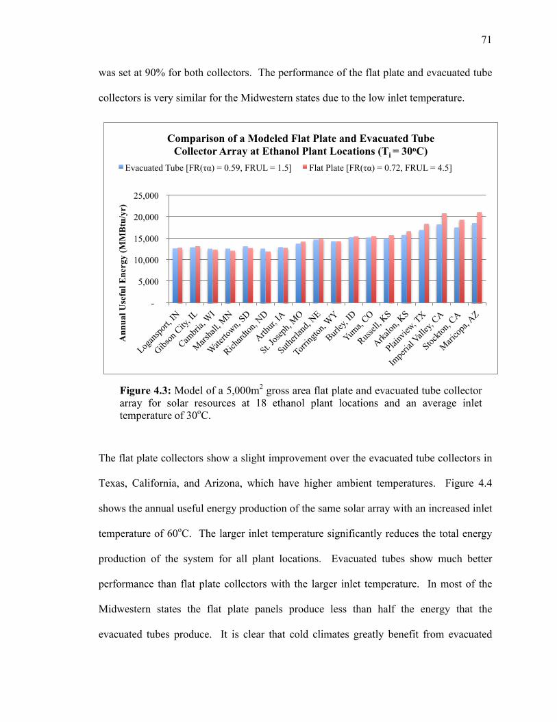
71
was set at 90% for both collectors. The performance of the flat plate and evacuated tube
collectors is very similar for the Midwestern states due to the low inlet temperature.
The flat plate collectors show a slight improvement over the evacuated tube collectors in
Texas, California, and Arizona, which have higher ambient temperatures. Figure 4.4
shows the annual useful energy production of the same solar array with an increased inlet
temperature of 60oC. The larger inlet temperature significantly reduces the total energy
production of the system for all plant locations. Evacuated tubes show much better
performance than flat plate collectors with the larger inlet temperature. In most of the
Midwestern states the flat plate panels produce less than half the energy that the
evacuated tubes produce. It is clear that cold climates greatly benefit from evacuated
-
5,000
10,000
15,000
20,000
25,000
Ann
ual U
sefu
l Ene
rgy
(MM
Btu
/yr)
Comparison of a Modeled Flat Plate and Evacuated Tube Collector Array at Ethanol Plant Locations (Ti = 30oC)
Evacuated Tube [FR(τα) = 0.59, FRUL = 1.5] Flat Plate [FR(τα) = 0.72, FRUL = 4.5]
Figure 4.3: Model of a 5,000m2 gross area flat plate and evacuated tube collector array for solar resources at 18 ethanol plant locations and an average inlet temperature of 30oC.
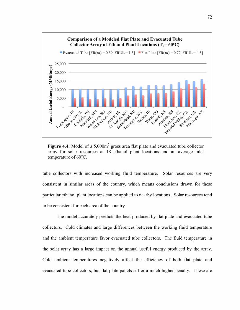
72
tube collectors with increased working fluid temperature. Solar resources are very
consistent in similar areas of the country, which means conclusions drawn for these
particular ethanol plant locations can be applied to nearby locations. Solar resources tend
to be consistent for each area of the country.
The model accurately predicts the heat produced by flat plate and evacuated tube
collectors. Cold climates and large differences between the working fluid temperature
and the ambient temperature favor evacuated tube collectors. The fluid temperature in
the solar array has a large impact on the annual useful energy produced by the array.
Cold ambient temperatures negatively affect the efficiency of both flat plate and
evacuated tube collectors, but flat plate panels suffer a much higher penalty. These are
-
5,000
10,000
15,000
20,000
25,000
Ann
ual U
sefu
l Ene
rgy
(MM
Btu
/yr)
Comparison of a Modeled Flat Plate and Evacuated Tube Collector Array at Ethanol Plant Locations (Ti = 60oC)
Evacuated Tube [FR(τα) = 0.59, FRUL = 1.5] Flat Plate [FR(τα) = 0.72, FRUL = 4.5]
Figure 4.4: Model of a 5,000m2 gross area flat plate and evacuated tube collector array for solar resources at 18 ethanol plant locations and an average inlet temperature of 60oC.

73
all proven facts in the solar thermal industry (IEA 2012), but this model demonstrates the
magnitude of these differences. Performance of a solar array depends on numerous input
variables that can all be changed to show the range of conditions that exist in during
actual operation.
4.4 Evaluating Model Results for Solar Thermal Projects
The total percent shift from natural gas heating to solar heating is very low for all
four situations considered above. The heating requirement for all of the ethanol plants
was assumed to be 29,000 Btu/gal-ethanol. The total percent shift to solar thermal energy
for the 5,000 m2 flat plate array with an inlet temperature of 30oC ranged between 0.4%
and 4.1%. Most of the locations had less than 1% shift to solar energy from natural gas.
These are very small percentages and may deter any further investigation, but total
percent shift is not a good measure of the total heating that could be accomplished by a
non-concentrating solar array.
Percent shift to solar heating for the boiler makeup water gives much more
reasonable values. The percent shift to solar heating of the boiler makeup water for the
array modeled in Figure 4.3 is shown in Figure 4.5 along with the total production
capacity for each ethanol plant. The largest percent shift is for the Torrington, WY plant
with an 87% shift. This very large percentage would be oversized for the 12 MGY plant,
because peak summer solar heating would most likely far exceed the plant’s makeup
water heating needs. All of the other plants show a more reasonable percent shift below
50%. Even with the low percent shift to solar heating, this array is quite substantial. The
gross area of the collectors is 5,000 m2 or just under 54,000 ft2. The actual installed array

74
would most likely be larger due to installation requirements. This is a large area, but
ethanol plants typically are built on many acres of land and have large flat roofs that
could be used for installing the solar array. It may be possible to install a larger array
depending on available area.
The payback periods for a flat plate and an evacuated tube array for all of the
ethanol plant locations were compared. Figure 4.6 shows the cumulative cost savings
over a lifespan of 30 years for a flat plate solar thermal array for six of the 18 ethanol
plants. Some manufacturers claim lifespans for solar thermal panels up to 30 years, but
20 years would be most common (IEA 2012). Thirty years are shown to represent the
maximum possible savings, but real operational lifetimes will most likely be shorter. The
modeled 5,000 m2 array had an estimated installed cost of $314/m2 with a government
rebate of 30%, which brought the installed cost down to $220/m2. The average inlet
temperature was set to 30oC. The initial natural gas price was set at $5/MMBtu, and an
Figure 4.5: Total plant capacity and percent shift to solar heating of the boiler makeup water using a 5,000 m2 flat plate array at 18 ethanol plants.
0
20
40
60
80
100
120
0%
20%
40%
60%
80%
100%
Plan
t Cap
acity
(MG
Y)
Perc
ent S
hift
to S
olar
Hea
ting
of M
akeu
p W
ater
Total Plant Capacity and Percent Shift to Solar Heating of the Makeup Water (5,000 m2 Flat Plate Array, Ti = 30oC) Percent Shift, %SMW Plant Capacity (MGY)

75
annual rate increase of 3.3% was chosen. A load factor of 90% was used to account for
additional heat losses and inefficiencies in the system. These six locations were chosen
to show the spread of the data. All of the plants not shown had payback periods between
the two extremes. Maricopa, AZ had the shortest payback period at about 9 years, while
Richardton, ND had the longest payback period at about 15 years. The efficiency of the
entire array was 58% for Maricopa and 44% for Richardton. This seemingly small
difference in efficiency had a large impact on the payback period and cumulative savings
of the two projects. The payback periods are quite far above the typical payback period
that businesses look for, but all of the solar arrays payback well before an expected
lifespan of 20 years and then continue to save energy and costs. The modeled array for
Maricopa, AZ provides a net profit of over $4 million with a 30-year lifespan. This is 4
-$1,500,000
-$500,000
$500,000
$1,500,000
$2,500,000
$3,500,000
$4,500,000
0 2 4 6 8 10 12 14 16 18 20 22 24 26 28 30
Cum
ulat
ive
Cos
t Sav
ings
Years After Installation
Cumulative Cost Savings Over System Lifespan for Flat Plate Solar Array at Various Locations
Maricopa, AZ Plainview, TX Arkalon, KS Yuma, CO Gibson City, IL Richardton, ND
Figure 4.6: Modeled cumulative cost savings of a standard flat plate solar array for selected ethanol plant locations. Model input values: FR(τα) = 0.72, FRUL= 4.5, Ti = 30oC, RNG = $5/MMBtu, nNG = 3.3%, ICs = $220/m2.
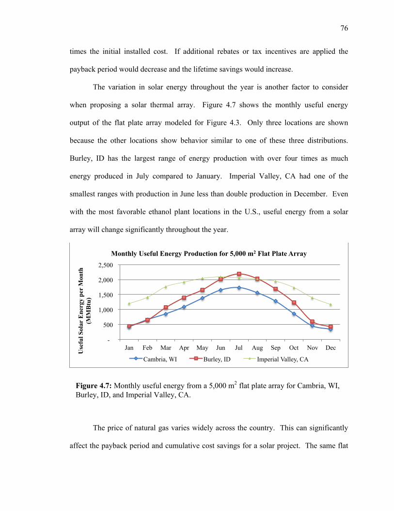
76
times the initial installed cost. If additional rebates or tax incentives are applied the
payback period would decrease and the lifetime savings would increase.
The variation in solar energy throughout the year is another factor to consider
when proposing a solar thermal array. Figure 4.7 shows the monthly useful energy
output of the flat plate array modeled for Figure 4.3. Only three locations are shown
because the other locations show behavior similar to one of these three distributions.
Burley, ID has the largest range of energy production with over four times as much
energy produced in July compared to January. Imperial Valley, CA had one of the
smallest ranges with production in June less than double production in December. Even
with the most favorable ethanol plant locations in the U.S., useful energy from a solar
array will change significantly throughout the year.
The price of natural gas varies widely across the country. This can significantly
affect the payback period and cumulative cost savings for a solar project. The same flat
-
500
1,000
1,500
2,000
2,500
Jan Feb Mar Apr May Jun Jul Aug Sep Oct Nov Dec
Use
ful S
olar
Ene
rgy
per
Mon
th
(MM
Btu
)
Monthly Useful Energy Production for 5,000 m2 Flat Plate Array
Cambria, WI Burley, ID Imperial Valley, CA
Figure 4.7: Monthly useful energy from a 5,000 m2 flat plate array for Cambria, WI, Burley, ID, and Imperial Valley, CA.

77
plate solar array modeled in Figure 4.6 was used to model the changes in payback period
due to adjustments to the natural gas price. All other variables were kept constant. The
average natural gas prices for California, Texas, Arizona, and Missouri for 2011 from
Table B.1 were used to more accurately model the payback period for solar arrays in
these states. The model results for both the U.S. average natural gas price of
$5.00/MMBtu and the average state natural gas prices for Imperial Valley, CA and
Plainview, TX are shown in Figure 4.8. The natural gas price for Texas is $4.11/MMBtu,
and the average price is $6.88/MMBtu for California. The payback periods and
cumulative cost savings for the Texas and California plants were very close for the
average U.S. gas price, but diverge when using the state gas rates. The payback period
for California went from just over 9 years to less than 7 years. The cumulative cost
savings increased by nearly $2 million. The lower natural gas rate in Texas increased the
payback period by two years and decreased the cumulative savings by over $800
-$1,500,000
$0
$1,500,000
$3,000,000
$4,500,000
$6,000,000
0 2 4 6 8 10 12 14 16 18 20 22 24 26 28 30
Cum
ulat
ive
Savi
ngs
Years of Installation
Comparison of Cumulative Savings for Adjustments to Natural Gas Rate (TX and CA)
I.V., CA ($5.00/MMBtu) I.V., CA ($6.88//MMBtu) TX ($5.00/MMBtu) TX ($4.11/MMBtu)
Figure 4.8: Modeled cumulative cost savings and payback period for Texas and California ethanol plants using the national and state natural gas prices. Model input values: FR(τα) = 0.72, FRUL= 4.5, Ti = 30oC, nNG = 3.3%, ICs = $220/m2.

78
thousand. The actual rate an ethanol plant pays for their natural gas use will be one of the
main determining factors in the profitability of a solar thermal array.
The rate paid for natural gas can makeup for sizeable differences in solar
resources. The modeled flat plate array in Figure 4.3 in Arizona produced over 30%
more energy than the same array in Missouri. By using the average natural gas prices in
Missouri and Arizona, the solar installation in Missouri is nearly as economical as the
installation in Arizona. Figure 4.9 shows the model results for the payback period and
cumulative savings for the national average natural gas rate and the state gas rate for the
solar array in Missouri and Arizona. The increased gas price of $8.24/MMBtu decreased
the payback period to less than 9 years, which is 4 years less than the payback period
using the national rate of $5/MMBtu. The cumulative savings increased by over $2
million as well. These values are all more favorable than the Arizona solar array using
the national gas rate. This shows that natural gas price can be a more important factor
-$1,500,000
$0
$1,500,000
$3,000,000
$4,500,000
$6,000,000
0 2 4 6 8 10 12 14 16 18 20 22 24 26 28 30
Cum
ulat
ive
Savi
ngs
Years After Installation
Comparison of Cumulative Savings for Adjustments to Natural Gas Rate (AZ and MO)
AZ ($5.00/MMBtu) AZ ($6.71/MMBtu) MO ($5.00/MMBtu) MO ($8.24/MMBtu)
Figure 4.9: Modeled cumulative cost savings and payback period for Arizona and Missouri ethanol plants using the national and state natural gas prices. Model input values: FR(τα) = 0.72, FRUL= 4.5, Ti = 30oC, nNG = 3.3%, ICs = $220/m2.

79
than solar resource in determining the economic feasibility of a solar thermal project.
The modeled array for Arizona becomes even more promising when the state gas rate of
$6.71/MMBtu is used. The payback period decreased to just over 7 years, which is a
reduction of 2 years. The cumulative savings over a 30-year lifespan of the solar array is
nearly $6 million. These results clearly show that accurate natural gas rates are
extremely important in determining the financial outcomes of a solar thermal project.
The cumulative savings can be slightly misleading because as the system ages it
will need more maintenance and replacement equipment. Some of the cost savings will
be used to maintain the system and make upgrades, but these costs should be significantly
less than the total savings per year. It is also not guaranteed that the system will still be
operating at an acceptable level after 30 years. It is likely that the efficiency of the
system will decrease slightly as the materials age as well. This will reduce the cost
savings predicted by the model. These are all factors to consider when planning for the
potential savings of a solar array.
The percent increase of natural gas prices will have a large influence on the
cumulative savings from a solar project, but does not reduce the payback period
significantly. Figure 4.10 shows the same flat plate array described for Figure 4.6 for
Maricopa, AZ with four different percent increases of the natural gas rate. The payback
period and cumulative cost savings are shown for a steady natural gas price of
$6.71/MMBtu over a 25 year lifespan as well as yearly rate increases of 2%, 3.33%, and
5%. The payback periods for the steady rate, 2% and 3.33% are all between 7 and 8
years, and the 5% rate increase shows a payback period of between 6 and 7 years. The
main difference between these rate increases is the total cost savings after about 12 years.

80
With a 5% rate increase, the cumulative cost savings are $3.2 million more than the
steady gas rate. This is almost three times the purchase price of the original system.
Very large values for the lifetime savings of a solar array are possible if the price of
natural gas increases at a high rate. As discussed previously, a 2% yearly rate increase in
current dollars is the most likely future scenario. If inflation were considered, then the
3.33% value would be more realistic. The yearly price increase of natural gas will mostly
likely be a secondary consideration when planning a solar project. Its minimal effect on
payback period means that it is not essential when considering short timeframes. Future
natural gas prices should be considered when the lifetime profitability of a system is
analyzed.
All of the simulations of payback periods shown previously used the low installed
cost estimate of $314/m2 for flat plate collectors with a 30% government incentive. The
Figure 4.10: Modeled cumulative cost savings and payback period for a flat plate array in Maricopa, AZ with four different percent price increases for natural gas. Model input values: FR(τα) = 0.72, FRUL= 4.5, Ti = 30oC, ICs = $220/m2.
-$1,500,000
$0
$1,500,000
$3,000,000
$4,500,000
$6,000,000
0 1 2 3 4 5 6 7 8 9 10 11 12 13 14 15 16 17 18 19 20 21 22 23 24 25
Cum
ulat
ive
Cos
t Sav
ings
Years After Installation
Cumulative Cost Savings for Solar Array in Maricopa, AZ with Various Natural Gas Rate Increases
5% 3.33% 2% 0%

81
30% federal government incentive is currently available for solar thermal systems
through the year 2016 (DSIRE 2012), so it will be considered for all simulations.
Payback periods for the low and high costs of flat plate and evacuated tube collectors are
compared for a 5,000 m2 gross area solar array in Sutherland, NE in Figure 4.11. The
input variables for the model are shown in Table 4.1. The load factor for the flat plate
-$2,000,000
-$1,500,000
-$1,000,000
-$500,000
$0
$500,000
$1,000,000
0 1 2 3 4 5 6 7 8 9 10 11 12 13 14 15 16 17 18 19 20
Cum
ulat
ive
Cos
t Sav
ings
Years After Installation
Comparison of Payback Periods for Low and High Installed Costs for Flat Plate and Evacuated Tube Arrays in Sutherland, NE
FP, Low Price ET, Low Price FP, High Price ET, High Price
Table 4.1: Model inputs for simulation shown in Figure 4.11 for different installed costs
Price Inputs
Flat Plate Evacuated Tube Current Average Price of Natural Gas for Industrial
Sector, RNG ($/MMBtu) 5.44 5.44
Natural Gas Percent Price Increase per Year, nNG 0.033 0.033 Solar Inputs
Total Area of Each Collector, AT (m2) 5 5 Number of Panels, Np 1000 1000
Price per square meter, ICsc ($/m2) $220 / 293 $293 / 391 FR(τα)n 0.72 0.59
FRUL (W/m2-oC) 4.5 1.5 Input temperature of working fluid, Ti (oC) 35 35
Load Factor, Lf 0.85 0.9
Figure 4.11: Modeled cumulative savings and payback period for low and high installed costs for a standard flat plate and evacuated tube collector array in Sutherland, NE.

82
array is 5% lower than the evacuated tube array to account for reduced absorption when
the sun is low in the sky. The average natural gas price for Nebraska of $5.44/MMBtu
was used. The low-priced flat plate collector had the shortest payback period at 13 years
while the low-priced evacuated tube collector was at 15 years, the high priced flat plate
collector was at 16 years, and the high priced evacuated tube was at 19 years. All of
these payback periods are most likely too long to be considered economically feasible for
an ethanol plant. The low-priced evacuated tube collector begins to draw nearer the low-
priced flat plate collector as more years pass. The increased solar energy available from
the evacuated tube collector begins to make up for the high installed cost, but doesn’t
reach the cumulative savings of the flat plate collector until after 20 years.
This model can also be used with yearly averages for the solar insolation and
ambient air temperature. The model outputs using the monthly data and yearly averages
for several plant locations were compared to see the differences between these two
methods. Table 4.2 shows the useful energy output of the model for the inputs shown in
Table 4.1 with a load factor of 90%. The table shows the model outputs for the yearly
and monthly inputs as well as the percent difference in these values. The monthly
Table 4.2: Comparison of model outputs for monthly and yearly data inputs
Location Useful Energy
MMBtu/yr (Yearly Inputs)
Useful Energy MMBtu/yr
(Monthly Inputs)
Percent Difference
Marshall, MN 10,376 10,763 3.6% Gibson City, IL 11,531 11,846 2.7% St. Joseph, MO 12,606 12,890 2.2%
Arkalon, KS 15,108 15,308 1.3% Maricopa, AZ 19,577 19,758 0.9%

83
meteorological data inputs give a slightly higher value for useful energy and the
difference increases as the yearly range in air temperature and solar energy increases.
The model only shows small differences for monthly and yearly data inputs and should
not have a substantial effect on the final output values.
The payback period for a realistic flat plate array was modeled using the
individual state natural gas prices for all of the ethanol plant locations. All of the input
values for the flat plate collector from Table 4.1 were used except the load factor. The
load factor was increased to 90% to model a well-designed system with minimal losses.
The lower installed cost of $220/m2 was used because the size of the system should
provide savings in bulk discounts on equipment, and the 30% Investment Tax Credit
(ITC) was applied. Table 4.3 shows the natural gas price and the payback period for this
Table 4.3: State natural gas rates and payback period modeled for a realistic flat plate collector
Location Natural Gas Price ($/MMBtu)
Payback Period
First Year Cost Savings, SS ($/yr)
Logansport, IN 5.52 14.0 $63,331 Gibson City, IL 6.59 11.8 $78,065
Cambria, WI 6.79 12.2 $74,704 Marshall, MN 5.44 14.9 $58,551
Watertown, SD 5.89 13.3 $67,117 Richardton, ND 4.97 16.1 $52,657
Arthur, IA 5.71 13.6 $65,362 St. Joseph, MO 8.24 9.1 $106,214 Sutherland, NE 5.44 12.4 $73,435 Torrington, WY 4.8 14.1 $62,242
Burley, ID 6.25 10.6 $88,250 Yuma, CO 5.71 11.4 $80,985 Russell, KS 5.38 11.8 $77,542 Arkalon, KS 5.38 11.2 $82,357
Plainview, TX 4.11 12.9 $69,911 Imperial Valley, CA 6.88 7.4 $134,057
Stockton, CA 6.88 7.9 $123,613 Maricopa, AZ 6.71 7.5 $132,576

84
array for all of the ethanol plant locations. Only three states have payback periods less
than ten years, which include Arizona, California, and Missouri. These three states are
the best locations to consider a solar thermal array. California and Arizona have ample
solar resources with mid-range natural gas prices to provide payback periods less than 8
years. Missouri is a good candidate for a solar array due to moderate solar resources and
a high natural gas price. All three states have yearly natural gas cost savings over
$100,000 for the first year. Solar thermal systems could be practical in Idaho, Kansas,
and Colorado if additional incentives are available through federal and local programs. If
substantial financial assistance and backing for solar thermal projects becomes available
through additional government programs, then a flat plate array may become feasible for
most of the other ethanol plant locations. It is unlikely that any amount of financial
assistance would make a solar thermal array practical for an ethanol plant in North
Dakota due to the low solar resources and low natural gas price.
The model accurately estimates the payback period and cumulative cost savings
for solar thermal projects. Changes to the numerous inputs can model a wide range of
project conditions to compare different possibilities. The cost of natural gas has a very
large influence on project feasibility while solar resources generally have a smaller
influence. Variations in the yearly price increase of natural gas mainly influence the
lifetime savings of a project, but do not change the payback period significantly.
Continued government incentives are essential to the feasibility of future solar hot water
heating projects for ethanol plants.
Solar thermal arrays can be a viable option for ethanol plants to reduce energy
costs, fossil fuel consumption, and greenhouse gas emissions. There are some financial

85
risks due to the large installed cost of the system and the long payback periods. The most
profitable solar arrays will be in areas with medium to high solar resources with natural
gas rates well above the national average. Expanded government incentives and
programs could make solar heating profitable for Midwestern states where most of the
corn ethanol is produced. It is unlikely that solar thermal projects will be economically
viable for the most northern states due to extreme temperatures and lower solar resources.
4.5 Verifying the Wind Energy Model
The wind model was verified by comparing the electricity generation of the
modeled turbines for the various ethanol plant locations to average data from installed
projects across the country. The model inputs are shown in Table 4.4 as well as the
outputs for the design turbine using a power coefficient (Cpd) of 0.5. The design power
coefficient was used to find the design turbine power and theoretical electricity
generation to determine the actual capacity factor. The model outputs for the electricity
generation of this turbine at the various ethanol plant locations is shown in Table 4.5
Table 4.4: Model inputs for a standard wind turbine with the outputs for the design turbine with Cpd = 0.5.
Wind Inputs Input
Design Wind Speed for Turbine, Vd (m/s) 9.8 Installed Cost of Wind Turbine, ICwt ($/kW) 1800
Diameter of Turbine Blade, DR (m) 81 Monthly Wind Data
Input Power Coefficient, Cpa or Cpd 0.45
Capacity Factor, 1 or Cfa 0.95 Outputs Output
Design Turbine Power, Pd (MW) 1.5 Theoretical Electricity Generation, Ewt (kWh/yr) 13,140,000
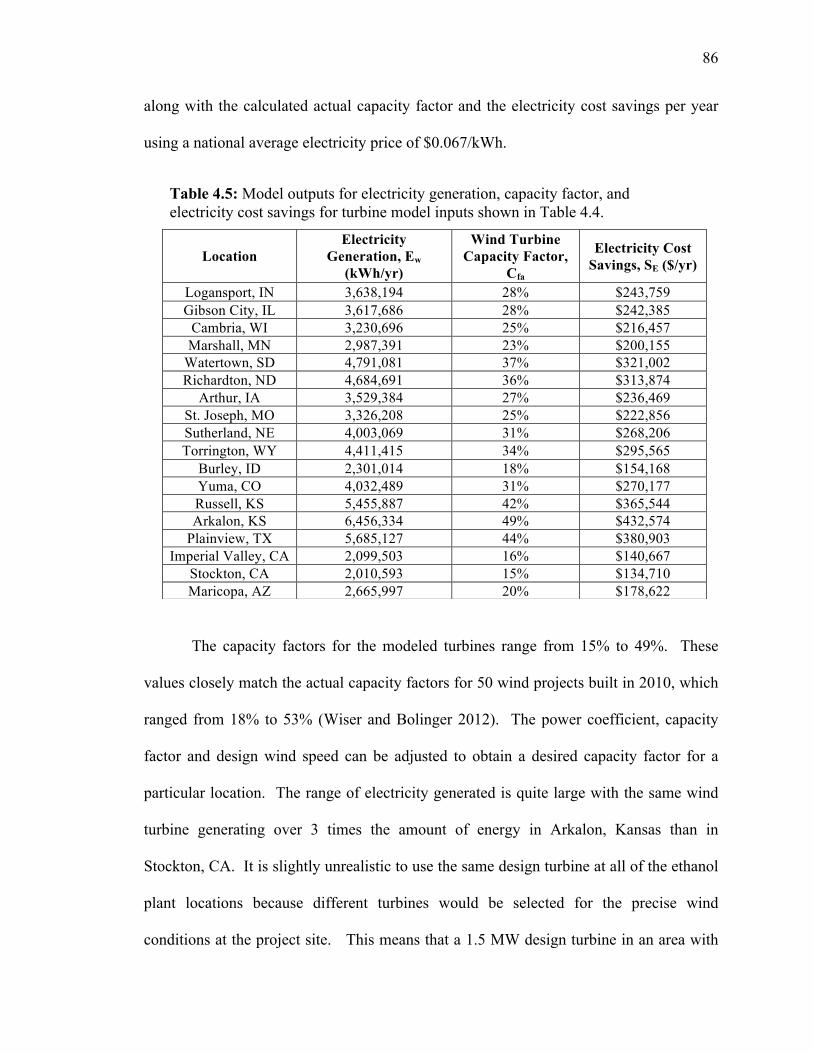
86
along with the calculated actual capacity factor and the electricity cost savings per year
using a national average electricity price of $0.067/kWh.
The capacity factors for the modeled turbines range from 15% to 49%. These
values closely match the actual capacity factors for 50 wind projects built in 2010, which
ranged from 18% to 53% (Wiser and Bolinger 2012). The power coefficient, capacity
factor and design wind speed can be adjusted to obtain a desired capacity factor for a
particular location. The range of electricity generated is quite large with the same wind
turbine generating over 3 times the amount of energy in Arkalon, Kansas than in
Stockton, CA. It is slightly unrealistic to use the same design turbine at all of the ethanol
plant locations because different turbines would be selected for the precise wind
conditions at the project site. This means that a 1.5 MW design turbine in an area with
Table 4.5: Model outputs for electricity generation, capacity factor, and electricity cost savings for turbine model inputs shown in Table 4.4.
Location Electricity
Generation, Ew (kWh/yr)
Wind Turbine Capacity Factor,
Cfa
Electricity Cost Savings, SE ($/yr)
Logansport, IN 3,638,194 28% $243,759 Gibson City, IL 3,617,686 28% $242,385
Cambria, WI 3,230,696 25% $216,457 Marshall, MN 2,987,391 23% $200,155
Watertown, SD 4,791,081 37% $321,002 Richardton, ND 4,684,691 36% $313,874
Arthur, IA 3,529,384 27% $236,469 St. Joseph, MO 3,326,208 25% $222,856 Sutherland, NE 4,003,069 31% $268,206 Torrington, WY 4,411,415 34% $295,565
Burley, ID 2,301,014 18% $154,168 Yuma, CO 4,032,489 31% $270,177 Russell, KS 5,455,887 42% $365,544 Arkalon, KS 6,456,334 49% $432,574
Plainview, TX 5,685,127 44% $380,903 Imperial Valley, CA 2,099,503 16% $140,667
Stockton, CA 2,010,593 15% $134,710 Maricopa, AZ 2,665,997 20% $178,622

87
lower wind speeds might have a 90 m rotor diameter while a 1.5 MW turbine in an area
with higher wind speeds could have a rotor diameter of only 75 m. In such a case, the
turbine with the larger rotor will most likely cost more and have a longer payback period.
These two opposing factors allow the comparison of the same turbine to be valid for
areas with differing wind speeds. Comparisons between the locations for the same
turbine are meant to be general and a more thorough analysis would require considering
different design turbines for different areas.
4.6 Evaluating Model Results for Wind Projects
The wind model can be used to evaluate a large range of project conditions to
determine the economic feasibility of installing a wind turbine at an ethanol plant. The
18 ethanol plant locations were evaluated to determine if they provided a favorable
opportunity for wind power development. Several input variables were changed to
analyze the impact on payback period and cumulative cost savings.
Figure 4.12 shows the annual electricity production values from Table 4.5 for a
1.5 MW turbine and the annual average wind speed at each plant location. The large
variation in electricity production for relatively small changes in wind speed can be
clearly seen.
Installing a wind turbine can replace a substantial percentage of the total
electricity needs of an ethanol plant. For this model an electricity requirement of 0.74
kWh/gal-ethanol was used. The 1.5 MW turbine modeled with input variables shown in
Table 4.4 replaces between 4% and 50% of the electricity needs of the various ethanol
plants. The percent shift to wind power and the individual plant capacity is shown in

88
Figure 4.13 for each ethanol plant. This turbine may be slightly oversized for the
Wyoming plant due to the large installed cost, but there is no issue with wasted energy
with a wind turbine. The turbine is connected to the electrical grid so the next customers
down the line would use any excess energy. To attain a higher percent shift to wind
power a larger turbine or multiple turbines could be installed. Contracts with a utility
company called a power purchase agreement (PPA) can be settled in which the utility
company will purchase all of the electricity generated by the turbine. This means there is
no penalty for consuming less energy than is produced by the turbine.
4 4.5 5 5.5 6 6.5 7 7.5 8 8.5
-
1,000,000
2,000,000
3,000,000
4,000,000
5,000,000
6,000,000
7,000,000
Aver
age
Win
d Sp
eed
(m/s
)
Ele
ctri
city
Gen
erat
ion
(kW
h/yr
)
Yearly Electricity Generation for a 1.5 MW Turbine and Average Wind Speed at Ethanol Plant Locations
Electricity Generation kWh/yr (Monthly Data) Average Wind Speed (m/s)
Figure 4.12: Average annual wind speed and electricity generation for a 1.5 MW turbine at different ethanol plant locations.

89
Wind speeds change throughout the year, which will modify the electricity
generated by the wind turbine. Typically wind speeds are lower in the summer and
higher in the winter. Understanding the differences in electricity generated throughout
the year will aid in project planning. Electricity rates are generally higher in the summer,
which means electricity generated during peak loads in the summer can be worth much
more than the same electricity generated during a winter night. Purchase agreements for
the electricity may have varying rates depending when it is generated. This will
influence payback periods and cumulative cost savings for the project. Figure 4.14
shows the monthly differences in electricity generation for a 1.5 MW turbine at four
ethanol plant locations. All of the locations have lower wind speeds during the summer,
but peak wind speeds differ between locations. The wind turbine in Wyoming produces
3 times the energy in January than July, and the turbine in Kansas generates double the
0
20
40
60
80
100
120
0%
10%
20%
30%
40%
50%
60%
Plan
t Cap
acity
(MG
Y)
Perc
ent S
hift
to W
ind
Pow
er
Total Plant Capacity and Percent Shift to Wind Power (1.5 MW Turbine)
Percent Shift, %SW Plant Capacity
Figure 4.13: Plant capacity and percent shift to wind power for a 1.5 MW turbine for each ethanol plant.

90
energy in April as compared to August. Most of the other locations have monthly
electricity variations similar to Kansas. The peak wind speeds occur in April and dip
dramatically in July and August. The rate differences between electricity generated
during peak demand periods should be considered when moving into secondary stages of
wind project planning.
The payback periods and cumulative lifetime savings for the 1.5 MW turbine
described in Table 4.4 were compared for all of the ethanol plant locations. The price
input variables and the installed cost output are shown in Table 4.6. The average U.S.
electricity rate is used along with an installed cost of $1,800/kW. No government
incentives were applied to the installed cost or electricity rate. A yearly electricity rate
increase of 2% was used to simulate inflation. This results in a total installed cost of $2.7
million. The payback periods ranged from less than 6 to over 16 years. It is clear that
there are several locations that are not ideal candidates for wind power. Figure 4.15
- 100,000 200,000 300,000 400,000 500,000 600,000 700,000 800,000 900,000
Jan Feb Mar Apr May Jun Jul Aug Sep Oct Nov Dec Mon
thly
Ele
ctri
city
Gen
erat
ion
(kW
h) Monthly Electricity Generation of a 1.5 MW Turbine
Richardton, ND Torrington, WY Arkalon, KS Maricopa, AZ
Figure 4.14: Monthly electricity generation for a 1.5 MW turbine in four locations.
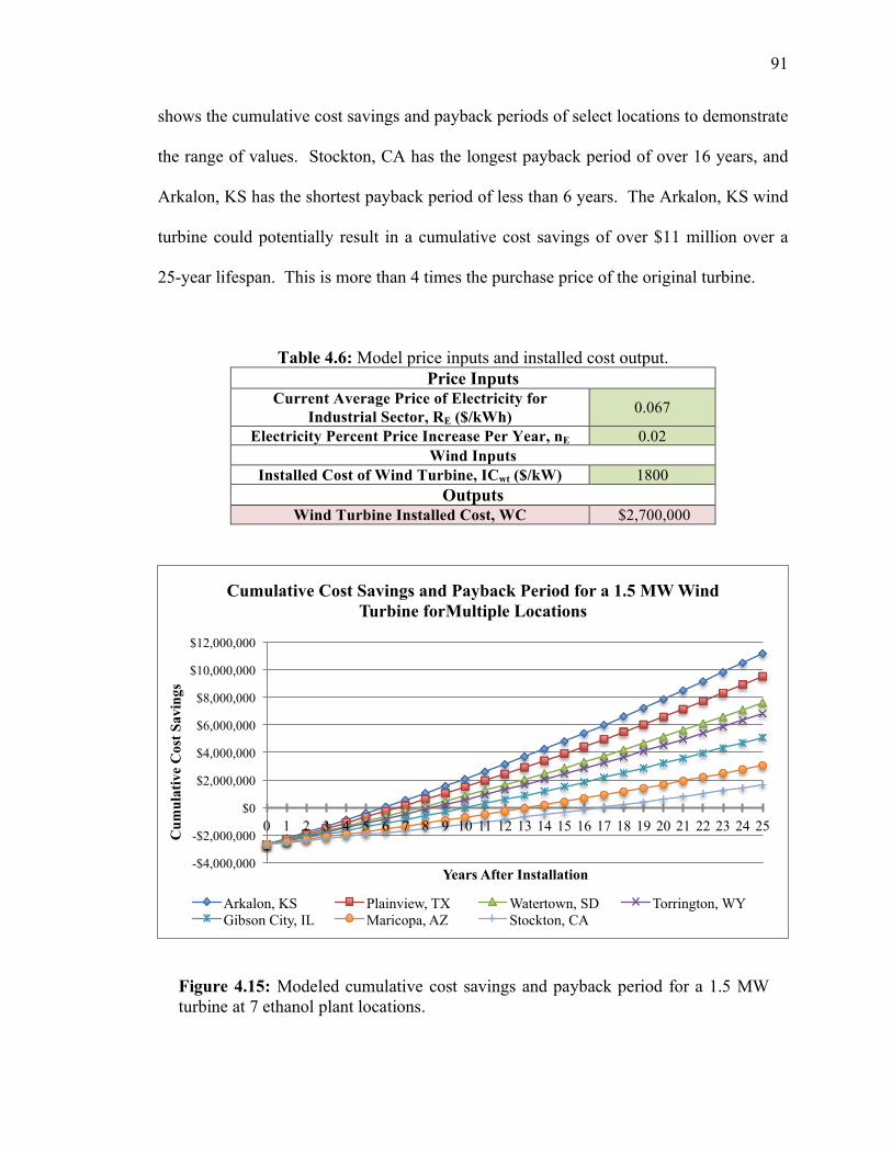
91
shows the cumulative cost savings and payback periods of select locations to demonstrate
the range of values. Stockton, CA has the longest payback period of over 16 years, and
Arkalon, KS has the shortest payback period of less than 6 years. The Arkalon, KS wind
turbine could potentially result in a cumulative cost savings of over $11 million over a
25-year lifespan. This is more than 4 times the purchase price of the original turbine.
Table 4.6: Model price inputs and installed cost output. Price Inputs
Current Average Price of Electricity for Industrial Sector, RE ($/kWh) 0.067
Electricity Percent Price Increase Per Year, nE 0.02 Wind Inputs
Installed Cost of Wind Turbine, ICwt ($/kW) 1800 Outputs
Wind Turbine Installed Cost, WC $2,700,000
-$4,000,000
-$2,000,000
$0
$2,000,000
$4,000,000
$6,000,000
$8,000,000
$10,000,000
$12,000,000
0 1 2 3 4 5 6 7 8 9 10 11 12 13 14 15 16 17 18 19 20 21 22 23 24 25
Cum
ulat
ive
Cos
t Sav
ings
Years After Installation
Cumulative Cost Savings and Payback Period for a 1.5 MW Wind Turbine forMultiple Locations
Arkalon, KS Plainview, TX Watertown, SD Torrington, WY Gibson City, IL Maricopa, AZ Stockton, CA
Figure 4.15: Modeled cumulative cost savings and payback period for a 1.5 MW turbine at 7 ethanol plant locations.

92
The values for payback period and cumulative savings shown in Figure 4.15 were
calculated using the average electricity rate $0.067/kWh, but many of the average state
rates for electricity differ significantly from this value. The payback period and
cumulative cost savings using the state and national rates for electricity were compared
for California and Wyoming in Figure 4.16. These two state electricity prices are far
from the average, which results in large changes in the economic favorability of these
two projects. The green curves show the cost savings for the national electricity rate, and
the blue curves show the cost savings for the state prices. Using Wyoming’s state
electricity rate increased the payback period by two years and the cumulative savings was
decreased by over $1.5 million. The payback period for the array in California was
reduced by 5 years and the cumulative savings increased by over $2 million by using the
average state electricity price. Using the correct state prices, the wind projects in
-$3,000,000
-$1,500,000
$0
$1,500,000
$3,000,000
$4,500,000
$6,000,000
0 1 2 3 4 5 6 7 8 9 10 11 12 13 14 15 16 17 18 19 20 21 22 23 24 25
Cum
ulat
ive
Cos
t Sav
ings
Years After Installation
Cumualative Cost Savings and Payback Period for a 1.5 MW Turbine for Differences in Electricity Rate
CA ($0.067/kWh) CA ($0.1011/kWh) WY ($0.067/kWh) WY ($0.0541/kWh)
Figure 4.16: Cumulative cost savings and payback period for a 1.5 MW wind turbine for the average state and national electricity rates for Wyoming and California.
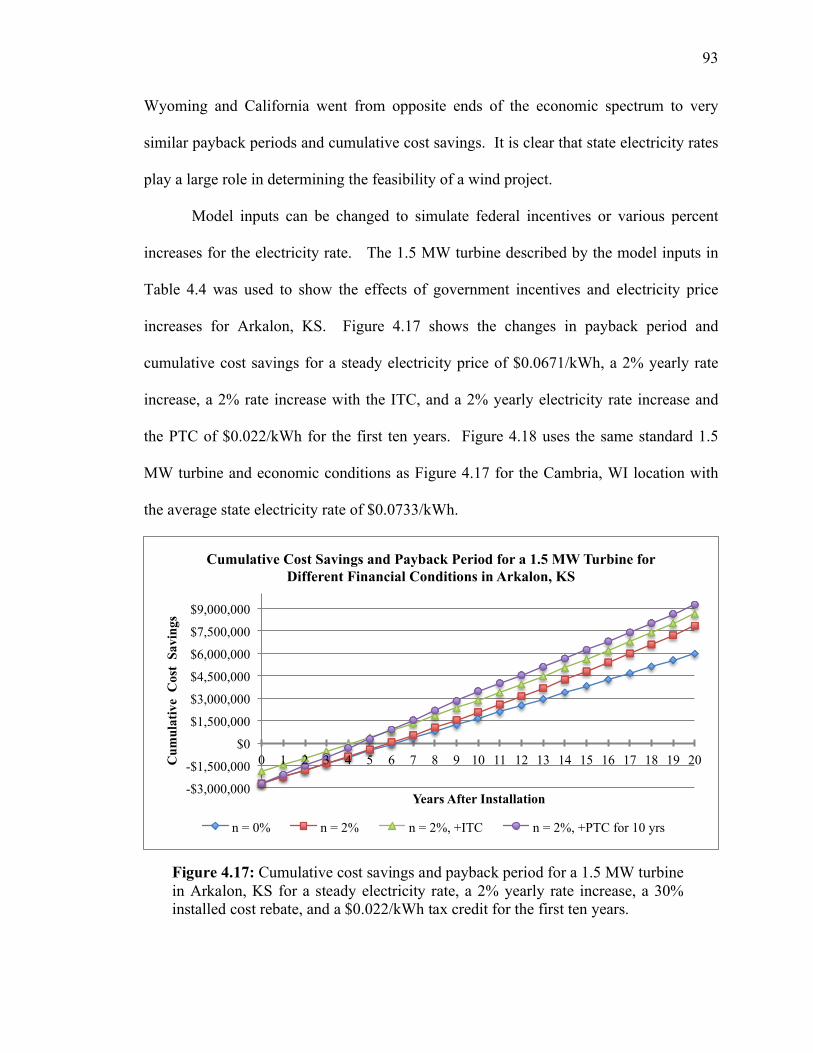
93
Wyoming and California went from opposite ends of the economic spectrum to very
similar payback periods and cumulative cost savings. It is clear that state electricity rates
play a large role in determining the feasibility of a wind project.
Model inputs can be changed to simulate federal incentives or various percent
increases for the electricity rate. The 1.5 MW turbine described by the model inputs in
Table 4.4 was used to show the effects of government incentives and electricity price
increases for Arkalon, KS. Figure 4.17 shows the changes in payback period and
cumulative cost savings for a steady electricity price of $0.0671/kWh, a 2% yearly rate
increase, a 2% rate increase with the ITC, and a 2% yearly electricity rate increase and
the PTC of $0.022/kWh for the first ten years. Figure 4.18 uses the same standard 1.5
MW turbine and economic conditions as Figure 4.17 for the Cambria, WI location with
the average state electricity rate of $0.0733/kWh.
-$3,000,000
-$1,500,000
$0
$1,500,000
$3,000,000
$4,500,000
$6,000,000
$7,500,000
$9,000,000
0 1 2 3 4 5 6 7 8 9 10 11 12 13 14 15 16 17 18 19 20 Cum
ulat
ive
Cos
t Sa
ving
s
Years After Installation
Cumulative Cost Savings and Payback Period for a 1.5 MW Turbine for Different Financial Conditions in Arkalon, KS
n = 0% n = 2% n = 2%, +ITC n = 2%, +PTC for 10 yrs
Figure 4.17: Cumulative cost savings and payback period for a 1.5 MW turbine in Arkalon, KS for a steady electricity rate, a 2% yearly rate increase, a 30% installed cost rebate, and a $0.022/kWh tax credit for the first ten years.
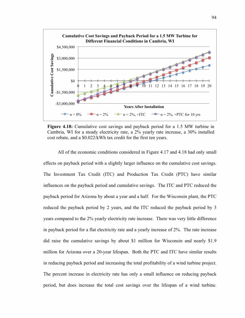
94
All of the economic conditions considered in Figure 4.17 and 4.18 had only small
effects on payback period with a slightly larger influence on the cumulative cost savings.
The Investment Tax Credit (ITC) and Production Tax Credit (PTC) have similar
influences on the payback period and cumulative savings. The ITC and PTC reduced the
payback period for Arizona by about a year and a half. For the Wisconsin plant, the PTC
reduced the payback period by 2 years, and the ITC reduced the payback period by 3
years compared to the 2% yearly electricity rate increase. There was very little difference
in payback period for a flat electricity rate and a yearly increase of 2%. The rate increase
did raise the cumulative savings by about $1 million for Wisconsin and nearly $1.9
million for Arizona over a 20-year lifespan. Both the PTC and ITC have similar results
in reducing payback period and increasing the total profitability of a wind turbine project.
The percent increase in electricity rate has only a small influence on reducing payback
period, but does increase the total cost savings over the lifespan of a wind turbine.
-$3,000,000
-$1,500,000
$0
$1,500,000
$3,000,000
$4,500,000
0 1 2 3 4 5 6 7 8 9 10 11 12 13 14 15 16 17 18 19 20
Cum
ulat
ive
Cos
t Sav
ings
Years After Installation
Cumulative Cost Savings and Payback Period for a 1.5 MW Turbine for Different Financial Conditions in Cambria, WI
n = 0% n = 2% n = 2%, +ITC n = 2%, +PTC for 10 yrs
Figure 4.18: Cumulative cost savings and payback period for a 1.5 MW turbine in Cambria, WI for a steady electricity rate, a 2% yearly rate increase, a 30% installed cost rebate, and a $0.022/kWh tax credit for the first ten years.
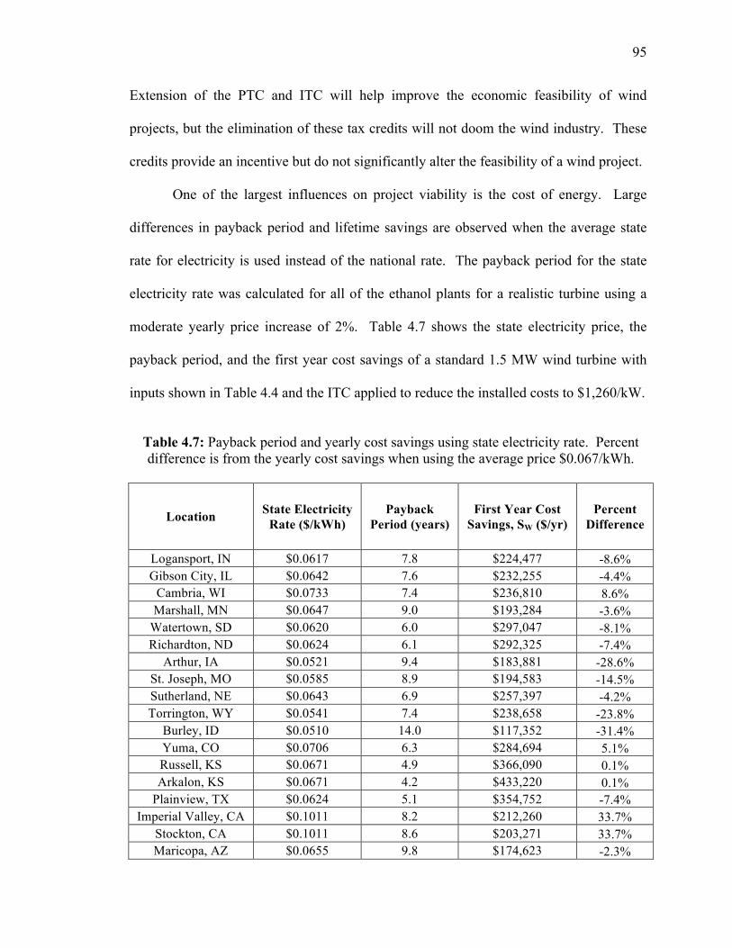
95
Extension of the PTC and ITC will help improve the economic feasibility of wind
projects, but the elimination of these tax credits will not doom the wind industry. These
credits provide an incentive but do not significantly alter the feasibility of a wind project.
One of the largest influences on project viability is the cost of energy. Large
differences in payback period and lifetime savings are observed when the average state
rate for electricity is used instead of the national rate. The payback period for the state
electricity rate was calculated for all of the ethanol plants for a realistic turbine using a
moderate yearly price increase of 2%. Table 4.7 shows the state electricity price, the
payback period, and the first year cost savings of a standard 1.5 MW wind turbine with
inputs shown in Table 4.4 and the ITC applied to reduce the installed costs to $1,260/kW.
Table 4.7: Payback period and yearly cost savings using state electricity rate. Percent difference is from the yearly cost savings when using the average price $0.067/kWh.
Location State Electricity Rate ($/kWh)
Payback Period (years)
First Year Cost Savings, SW ($/yr)
Percent Difference
Logansport, IN $0.0617 7.8 $224,477 -8.6% Gibson City, IL $0.0642 7.6 $232,255 -4.4%
Cambria, WI $0.0733 7.4 $236,810 8.6% Marshall, MN $0.0647 9.0 $193,284 -3.6%
Watertown, SD $0.0620 6.0 $297,047 -8.1% Richardton, ND $0.0624 6.1 $292,325 -7.4%
Arthur, IA $0.0521 9.4 $183,881 -28.6% St. Joseph, MO $0.0585 8.9 $194,583 -14.5% Sutherland, NE $0.0643 6.9 $257,397 -4.2% Torrington, WY $0.0541 7.4 $238,658 -23.8%
Burley, ID $0.0510 14.0 $117,352 -31.4% Yuma, CO $0.0706 6.3 $284,694 5.1% Russell, KS $0.0671 4.9 $366,090 0.1% Arkalon, KS $0.0671 4.2 $433,220 0.1%
Plainview, TX $0.0624 5.1 $354,752 -7.4% Imperial Valley, CA $0.1011 8.2 $212,260 33.7%
Stockton, CA $0.1011 8.6 $203,271 33.7% Maricopa, AZ $0.0655 9.8 $174,623 -2.3%

96
The percent difference between the yearly cost savings using the average rate of
$0.067/kWh and the state average rate is shown in the last column. These values were
chosen to give realistic but advantageous conditions for the installation of a wind turbine
at the various ethanol plant locations.
Wind turbines are economically feasible at most ethanol plant locations. All of
the ethanol plants except Idaho show payback periods less than 10 years. Texas and
Kansas are the ideal locations for wind development due to high wind resources and
moderate electricity rates. Both states have payback periods approximately 5 years or
less. A 5-year payback period would be in the realm of possibility for most businesses
due to lower financial risk. Colorado, North Dakota, and South Dakota are also good
locations for wind development. All three states had payback periods less than 6.5 years.
Projects in Indiana, Illinois, Wisconsin, and Wyoming would be slightly more risky with
payback periods between 7 and 8 years, but would result in significant energy and cost
savings for the ethanol plant. Wind projects could be economically feasible at all the
other ethanol plant locations if additional incentives are available or electricity rates are
higher at the plant’s location than the state average. Wind power is a financially
responsible choice that can provide energy and cost savings for ethanol plants across the
country. The specific economic and wind resource conditions at each ethanol plant will
ultimately determine how profitable a wind turbine would be.
This model can use either monthly or yearly wind resource data to provide energy
and cost savings estimates. Model outputs for all of the ethanol plants using monthly and
yearly data were compared to show if any errors were introduced between the methods.
Table 4.8 shows the yearly averaged wind speed, the electricity generation using monthly

97
and yearly data, and the percent difference between the values. All the values calculated
from monthly data are larger than the values calculated from the yearly average, but the
differences are small. The largest percent difference is 4.5% and the smallest is only
0.4%. Yearly wind speeds can be used for this calculation with only small errors
introduced. Since all of the calculations slightly underestimate turbine electricity
generation, the use of yearly wind speeds will give a more conservative estimate of the
power produced from the wind turbine.
This model can accurately estimate the payback period and cumulative cost
savings of a wind turbine. Adjustments to turbine parameters and price inputs can show
Table 4.8: Comparison of model outputs for monthly and yearly data inputs.
Location Average
Wind Speed (m/s)
Electricity Generation
kWh/yr (Monthly Data)
Electricity Generation
kWh/yr (Yearly Data)
Percent Difference
Logansport, IN 6.64 3,638,194 3,474,397 4.5% Gibson City, IL 6.63 3,617,686 3,458,724 4.4%
Cambria, WI 6.42 3,230,696 3,140,367 2.8% Marshall, MN 6.27 2,987,391 2,925,350 2.1%
Watertown, SD 7.36 4,791,081 4,731,607 1.2% Richardton, ND 7.31 4,684,691 4,635,829 1.0%
Arthur, IA 6.61 3,529,384 3,427,517 2.9% St. Joseph, MO 6.47 3,326,208 3,214,313 3.4% Sutherland, NE 6.92 4,003,069 3,932,725 1.8% Torrington, WY 7.1 4,411,415 4,247,665 3.7%
Burley, ID 5.78 2,301,014 2,291,705 0.4% Yuma, CO 6.92 4,032,489 3,932,725 2.5% Russell, KS 7.67 5,455,887 5,355,023 1.8% Arkalon, KS 8.13 6,456,334 6,377,448 1.2%
Plainview, TX 7.79 5,685,127 5,610,320 1.3% Imperial Valley, CA 5.58 2,099,503 2,061,949 1.8%
Stockton, CA 5.47 2,010,593 1,942,394 3.4% Maricopa, AZ 6.04 2,665,997 2,615,087 1.9%

98
the wide range of project possibilities. Small adjustments to wind speed and the cost of
electricity have a large effect on the profitability of a wind project. The addition of
government incentives and yearly electricity rate increases has a small influence on
payback periods and a slightly larger effect on the lifetime cost savings of a turbine.
Wind turbines can be a very smart investment for many ethanol plants throughout
the country. Payback periods will generally be under 10 years with a few locations under
5 years. Lifetime cost savings of a wind turbine can be 3 times the installed cost or more.
Specific conditions at the ethanol plant location will determine how favorable a wind
project will be.
4.7 Summary
This model accurately estimates the performance and cost savings of a solar array
and a wind turbine. Changes to input variables can model a wide range of project
conditions and have differing effects on model outputs. The economic feasibility of a
solar array and wind turbine was investigated for 18 ethanol plant locations across the
county. Solar thermal arrays and wind turbines are economically favorable for several
ethanol plant locations. Wind power is generally more realistic due to a more established
market and sufficient wind resources at many of the ethanol facilities across the U.S.
Government incentives will continue to play a role in the economics of renewable energy
projects.

99
CHAPTER 5: CONCLUSIONS AND RECOMMENDATIONS
5.1: Conclusions
Ethanol production plants are often in excellent locations for the application of
solar thermal and wind projects. The rural setting of most ethanol plants provides ample
space for a solar or wind installation with fewer logistical concerns than more populated
areas. Corn ethanol production is predicted to increase slightly over the next 20 years to
fulfill the RFS requirements, which ensures the market for ethanol will be strong in the
foreseeable future. The use of renewable energy sources will reduce the fossil fuel
consumption in the production of this renewable fuel. Ethanol’s opponents cite the large
energy requirements and the use of fossil fuel as two of the main arguments against corn
ethanol. Wind and solar energy can help meet the needs of certain ethanol plants across
the U.S.
Wind and solar projects can shift a significant amount of the energy burden from
conventional fossil fuels to renewable sources. The results of the modeling show that
when only the boiler makeup water is considered, a large solar thermal collector array
can shift about 10% of this heating requirement for the largest ethanol plants in the
country. A utility scale wind turbine can also provide 10% of the electricity requirements
of the largest ethanol facilities. Much larger shifts to renewable energy are possible for
smaller ethanol plants or larger solar and wind projects.
Solar thermal projects are most profitable in the Southwest, but high natural gas
prices can dramatically improve the economics of a solar thermal array. California and
Arizona are ideal locations for solar thermal projects, but very few ethanol plants are

100
located in these states. Missouri is home to a larger number of ethanol plants and has a
high natural gas price, which vastly improves the profitability of a solar array in this state.
Solar thermal systems in other states are generally only feasible if the actual natural gas
rate paid by the plant is well above the state’s average rate.
The profitability of solar thermal arrays depends greatly on government incentives.
The Investment Tax Credit (ITC) reduces net installed costs, which decreases the
payback period and allows solar projects to be more profitable. Payback periods are
generally long for solar thermal systems even in areas with high solar resources and
anything that can keep these timeframes lower will help build the industry.
Wind turbines are a very attractive option for reducing electricity consumption at
ethanol plants. Most of the ethanol plants in the U.S. are located throughout the Midwest,
which is where the largest wind resources are available. The wind industry is growing
rapidly and is expected to continue this growth for the next 20 years. Installed costs and
operation and maintenance costs are coming down, which improves project profitability.
Some areas of the country can achieve payback periods less than 5 years for a utility scale
turbine using the ITC. Higher electricity rates or larger wind speeds can reduce this
payback period further. Even without government incentives, wind turbines can have
reasonable payback periods and large lifetime cost savings. Neither the ITC nor the
Production Tax Credit (PTC) significantly changed the profitability of the wind projects
considered.
The wind resource values used for this model were regional averages and may not
accurately represent wind speeds at each ethanol plant location. Wind speed can

101
dramatically change the economics of a wind project, so accurate values are essential in
determining the economic feasibility of a wind project.
The profitability of a wind turbine is much higher than a solar thermal project for
almost every ethanol plant location. The only exceptions are California, Arizona, and
Idaho. However, these three states contain very few ethanol plants.
Both wind and solar projects are highly sensitive to changes in the price of energy.
It is not sufficient to use national averages for industrial electricity and natural gas prices.
State averages better represent the economics of a wind or solar project, but the energy
prices for a specific plant will give a better estimate of payback period and lifetime
savings. The electricity rate an ethanol plant is charged may not be the price they will be
paid for electricity generated. Power price agreements (PPA) can be signed to determine
how much the utility will pay for the electricity generated by a wind turbine. This value
may be more or less (typically less) than what the plant pays for electricity.
The model results show only small differences when monthly and yearly resource
inputs are used. Either method will give similar results, but a yearly average of solar
insolation or wind speed will not accurately represent the monthly differences in the
resource. Resource amounts can vary by up to 400% for some areas of the country.
Energy prices may change throughout the year, so it is valuable to know when the solar
or wind project will have low and high output.
Rate increases for electricity and natural gas do not have a large effect on payback
periods. While predicting the future price of energy is not essential to get an accurate
estimate of the payback period of a wind or solar project, energy rate increases can
significantly increase the lifetime cost savings of a project.

102
This model is meant to aid in the beginning stages of a solar thermal or wind
project, but is not intended to be a complete representation of all the factors that must be
considered when planning a renewable energy project. There are several key aspects that
are not addressed by this model. The cost of debt and specifically the interest on loans
acquired to install the renewable energy project are not considered in the calculation of
payback period or cost savings. This could influence the economics of the project.
Operation and maintenance (O&M) costs can be included in the model by reducing the
price of energy, but there are no specific methods to account for additional maintenance
costs as the system ages or specific inputs to calculate these costs separately. Generally
O&M costs are significantly lower than the yearly savings of the system, but these costs
may influence payback period and lifetime project savings. The model also does not
account for the depreciation of the wind turbine or solar array. A business owner may be
able to claim the depreciation of the renewable energy project as a tax deduction, which
would improve the finances of the project as a whole.
5.2 Recommendations
This model can provide valuable information to ethanol plants regarding the
feasibility of a renewable energy project at their respective locations. Information from
this research can be used to initiate a project or merely gain more information about wind
and solar energy. Ethanol plants can reduce fossil fuel consumption, greenhouse gas
emissions, and improve their public image by installing a renewable energy project.
Renewable energy projects are not only good for the environment, but they provide a
company reliable cost savings for 20 years or more.

103
There are some improvements that would make the model more accurate, but
some of these changes may not be beneficial. The addition of separate O&M costs would
give a broader picture of project costs and improve the accuracy of the model. Additional
financial considerations including debt servicing and depreciation may not be appropriate
for this type of model. The intended use of this model is a preliminary planning tool.
Once the planning process has moved forward then all of the details of the specific
location and the financial standing of the company can be considered. These additions
may make the model too specific for users that may be just considering the idea of a
renewable energy project. The scale of the projects considered would require extensive
project planning with outside companies or firms, and they will aid the company with
individualized financial calculations.
Government incentives should be continued for solar thermal projects. The ITC
can significantly reduce the payback period for a solar thermal installation. This
incentive is not set to expire for solar thermal systems until 2016, but if panel prices do
not come down significantly in that time, the ITC should be extended. It will be difficult
for this industry to grow in the future without continued support or reduced equipment
prices.
The profitability of wind power does not depend on government incentives.
Many in the wind industry forecast very low sales if the PTC is not extended past 2012.
Sales will most likely decrease, but the tax credit does not drastically change the finances
of a wind turbine. Wind turbines will be profitable without this tax credit, but
eliminating it could stall growth in the near future. Long-term success of the wind
industry will not depend on such tax credits.
104
REFERENCES
Aden, Andy. 2007. “Water Usage for Current and Future Ethanol Production.” Southwest
Hydrology 6, 4: 22-23
http://www.swhydro.arizona.edu/archive/V6_N5/feature4.pdf.
American Coalition for Ethanol (ACE). 2005. “Fuel Economy Study.”
http://www.ethanol.org/pdf/contentmgmt/ACEFuelEconomyStudy_001.pdf
American Wind Energy Association (AWEA). 2012. “AWEA U.S. Wind Industry Thrid
Quarter 2012 Market Report.” AWEA Data Services. http://www.awea.org/
learnabout/publications/reports/AWEA-US-Wind-Industry-Market-Reports.cfm
Ayompe, L.M., A. Duffy, M. Mc Keever, M. Conlon, S.J. McCormack. 2011.
“Comparative field performance study of flat plate and heat pipe evacuated tube
collectors (ETCs) for domestic water heating systems in a temperate climate.”
Energy 36: 3370-3378
Clean Fuels Development Coalition (CFDC). 2010. “Ethanol Fact Book: A Compilation
of Information About Fuel Ethanol.” http://www.cleanfuelsdc.org/pubs/
documents/CFDC%202010%20Ethanol%20Fact%20Book.pdf
Database of State Incentives for Renewables & Efficiency (DSIRE). 2012. “Financial
Incentives.” Accessed Oct 2012. http://dsireusa.org/incentives/index.cfm
?EE=1&RE=1&SPV=0&ST=0§or=Commercial&technology=Wind&sh=1
Edenhofer, Ottmar, Ramon Pichs-Madruga, Youba Sokona, et. al. 2011. “IPCC Special
Report on Renewable Energy Sources and Climate Change Mitigation.”
Intergovernmental Panel on Climate Change (IPCC).

105
ENERCON GmbH. 2010. “ENERCON Wind Energy Converters-Product Overview.”
http://www.enercon.de/p/downloads/EN_Productoverview_0710.pdf
Farrell, Alexander E., Richard J. Plevin, Brian T. Turner, Andrew D. Jones, Michael
O’Hare, Daniel M. Kammen. 2006. “Ethanol Can Contribute to Energy and
Environmental Goals.” Science 311(5760): 506-508.
Fay, James A. and Dan S. Golomb. 2012. “Energy and the Environment – Scientific and
Technological Principles.” New York: Oxford University Press.
Global Wind Energy Council (GWEC). 2012. “Interactive Map.” Accessed Nov 6 2012
http://www.gwec.net/global-figures/interactive-map/
Institut für Solartechnik SPF (Institute for Solar Technology). 2012. SPF Online
Collector Catalogue. http://www.solarenergy.ch/Collectors.111.0.html?&L=6
International Energy Agency (IEA). 2012. “Technology Roadmap: Solar Heating and
Cooling.”
http://www.iea.org/publications/freepublications/publication/name,28277,en.html
International Energy Agency’s Solar Heating and Cooling Programme (IEA SHC). 2004.
“Recommendation: Converting Solar Thermal Collector area into installed
capacity (m2 to kWth).” Technical note from meeting proceedings, Gleisdorf,
Austria. September 8. http://www.iea.org/publications/freepublications/
publication/2012_SolarHeatingCooling_Roadmap_FINAL_WEB.pdf
Keeney, D.R., and T.H. DeLuca. 1992. “Biomass as an Energy Source for the
Midwestern U.S.” American Journal of Alternative Agriculture 7: 137-144
Knoll, Keith, et al. 2009. “Effects of Intermediate Ethanol Blends on Legacy Vehicles
and Small Non-road Engines, Report 1 – Updated.” NREL: NREL/TP-540-43543

106
Laylin, Tafline. 2012. “World’s Largest (Gargantuan) Solar Thermal Plant Opens in
Saudi Arabia.” Green Prophet. http://www.greenprophet.com/2012/04/worlds-
largest-solar-thermal-plant/
Liska, Adam J. et al. 2009. “Improvements in the Life Cycle Energy Efficiency and
Greenhouse Gas Emissions of Corn-Ethanol.” Journal of Industrial Ecology 13.1:
58-74
Mueller, Steffen. 2010. “Detailed Report: 2008 National Dry Mill Corn Ethanol Survey.”
University of Illinois at Chicago, Energy Resources Center.
http://www.ethanol.org/pdf/contentmgmt/Ethanol_production_efficiency_U_of_I
L_spring_2010.pdf.
National Renewable Energy Laboratory (NREL). 2012. http://www.nrel.gov/
Niven, Robert K. 2004. “Ethanol in Gasoline: Environmental Impacts and Sustainability
Review Article.” Renewable and Sustainable Energy Reviews 9: 535-555.
Perlack, Robert D. et al. 2005. “Biomass as Feedstock For Bioenergy and Bioproducts
Industry: The Technical Feasibility of a Billion-Ton Annual Supply.” DOE,
USDA: DOE/GO-102005-2135.
http://www1.eere.energy.gov/biomass/pdfs/final_billionton_vision_report2.pdf.
Pimentel, David. 2001. “Ethanol Fuels: Energy Balance, Economics, and Environmental
Impacts are Negative.” Natural Resources Research 12: 127-134.
Ragheb, Magdi and Adam M. Ragheb. 2011. “Wind Turbines Theory - The Betz
Equation and Optimal Rotor Tip Speed Ratio, Fundamental and Advanced Topics
in Wind Power.” Dr. Rupp Carriveau (Ed.), ISBN: 978-953-307-508-2, InTech.
http://www.intechopen.com/books/fundamental-and-advanced-topicsin-wind

107
power/wind-turbines-theory-the-betz-equation-and-optimal-rotor-tip-speed-ratio
Renewable Fuels Association (RFA). 2012a. “2012 Ethanol Industry Outlook.”
Renewable Fuels Association: Washington DC.
http://www.ethanolrfa.org/pages/annual-industry-outlook.
Renewable Fuels Association (RFA). 2012b. http://www.ethanolrfa.org/
RETScreen International. 2005. “RETScreen Software Online User Manual-Solar Water
Heating Project Model.” Natural Resources, Canada, www.retscreen.net.
RETScreen International. 2012. www.retscreen.net.
Roney, Matthew J. 2012. “Wind Tops 10 Percent Share of Electricity in Five U.S. States.”
Earth Policy Institute. http://www.earth-
policy.org/data_highlights/2012/highlights27
Stackhouse, Paul W. 2012. “Surface Meterorology and Solar Energy-A renewable energy
resource web site.” NASA, POWER: (release 6.0)
http://eosweb.larc.nasa.gov/cgi-bin/sse/sse.cgi?+s01#s01
Shapouri, Hosein, James A. Duffeild, and Michael S. Graboski. 2002. “The Energy
Balance of Corn Ethanol: An Update.” USDA, AER-813
Swofford, Jeff. 2010. “AWEA Conducts National Wind Energy Survey.” Energy Boom.
http://www.energyboom.com/wind/awea-conducts-national-wind-energy-survey
Tegen, S., M. Hand, B. Maples, E. Lantz, P. Schwabe, and A. Smith. 2010. “2010 Cost of
Wind Energy Review.” NREL: NREL/TP-5000-52920
U.S. Department of Agriculture (USDA), National Agricultural Statistics Service. 2012.
“Production by Country and Location of Ethanol Plants.”
108
http://www.nass.usda.gov/Charts_and_Maps/Ethanol_Plants/U._S._Ethanol_Plant
s/index
U.S. Department of Energy (DOE). 2008. "Biofuels & Greenhouse Gas Emissions:
Myths versus Facts." http://www.doe.gov/downloads/ethanol-myths-and-facts.
U.S. Department of Energy (DOE). 2012. “U.S. Consumption of Ethanol and MTBE
Oxygenates.” Alternative Fuels Data Center.
http://www.afdc.energy.gov/data/tab/all/data_set/10322.
U.S. Energy Information Administration (EIA). 2011. “International Energy Outlook
2011.” DOE,EIA: DOE/EIA-0484(2011).
U.S. Energy Information Administration (EIA). 2012a. “Annual Energy Outlook 2012:
With Projections to 2035.” DOE, EIA: DOE/EIA-0383(2012).
U.S. Energy Information Administration (EIA). 2012b. “Annual Energy Review 2011.”
DOE, EIA: DOE/EIA-0384(2011).
U.S. Energy Information Administration (EIA). 2012c. www.eia.gov
U.S. Environmental Protection Agency (EPA). 2012. “E15 (a blend of gasoline and
ethanol).” website www.epa.gov/otaq/regs/fuels/additive/e15.
Wang, Michael, May Wu, and Hong Huo. 2007. “Life-cycle Energy and Greenhouse Gas
Emission Impacts of Different Corn Ethanol Plant Types.” Environmental
Research Letters 2: 024001
Wiser, Ryan and Mark Bolinger. 2012. “2011 Wind Technologies Market Report.” DOE:
DOE/GO-102012-3472
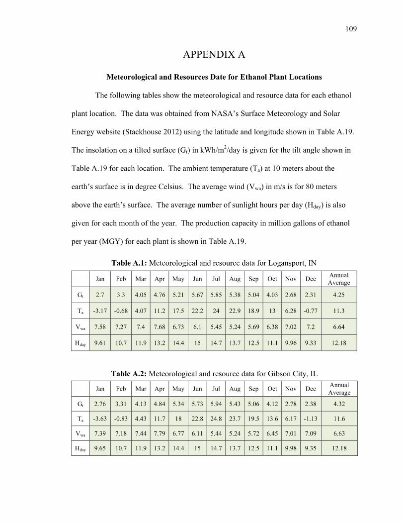
109
APPENDIX A
Meteorological and Resources Date for Ethanol Plant Locations
The following tables show the meteorological and resource data for each ethanol
plant location. The data was obtained from NASA’s Surface Meteorology and Solar
Energy website (Stackhouse 2012) using the latitude and longitude shown in Table A.19.
The insolation on a tilted surface (Gt) in kWh/m2/day is given for the tilt angle shown in
Table A.19 for each location. The ambient temperature (Ta) at 10 meters about the
earth’s surface is in degree Celsius. The average wind (Vwa) in m/s is for 80 meters
above the earth’s surface. The average number of sunlight hours per day (Hday) is also
given for each month of the year. The production capacity in million gallons of ethanol
per year (MGY) for each plant is shown in Table A.19.
Table A.1: Meteorological and resource data for Logansport, IN
Jan Feb Mar Apr May Jun Jul Aug Sep Oct Nov Dec Annual Average
Gt 2.7 3.3 4.05 4.76 5.21 5.67 5.85 5.38 5.04 4.03 2.68 2.31 4.25
Ta -3.17 -0.68 4.07 11.2 17.5 22.2 24 22.9 18.9 13 6.28 -0.77 11.3
Vwa 7.58 7.27 7.4 7.68 6.73 6.1 5.45 5.24 5.69 6.38 7.02 7.2 6.64
Hday 9.61 10.7 11.9 13.2 14.4 15 14.7 13.7 12.5 11.1 9.96 9.33 12.18
Table A.2: Meteorological and resource data for Gibson City, IL
Jan Feb Mar Apr May Jun Jul Aug Sep Oct Nov Dec Annual Average
Gt 2.76 3.31 4.13 4.84 5.34 5.73 5.94 5.43 5.06 4.12 2.78 2.38 4.32
Ta -3.63 -0.83 4.43 11.7 18 22.8 24.8 23.7 19.5 13.6 6.17 -1.13 11.6
Vwa 7.39 7.18 7.44 7.79 6.77 6.11 5.44 5.24 5.72 6.45 7.01 7.09 6.63
Hday 9.65 10.7 11.9 13.2 14.4 15 14.7 13.7 12.5 11.1 9.98 9.35 12.18
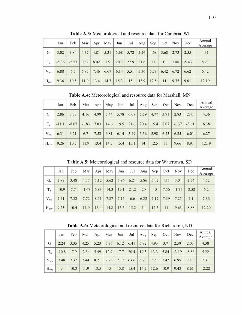
110
Table A.3: Meteorological and resource data for Cambria, WI
Jan Feb Mar Apr May Jun Jul Aug Sep Oct Nov Dec Annual Average
Gt 3.02 3.84 4.37 4.81 5.31 5.68 5.72 5.26 4.68 3.68 2.73 2.55 4.31
Ta -8.36 -5.51 0.32 8.02 15 20.7 22.9 21.6 17 10 1.88 -5.43 8.27
Vwa 6.88 6.7 6.87 7.46 6.67 6.14 5.51 5.36 5.78 6.42 6.72 6.62 6.42
Hday 9.36 10.5 11.9 13.4 14.7 15.3 15 13.9 12.5 11 9.75 9.01 12.19
Table A.4: Meteorological and resource data for Marshall, MN
Jan Feb Mar Apr May Jun Jul Aug Sep Oct Nov Dec Annual Average
Gt 2.86 3.38 4.16 4.99 5.44 5.78 6.07 5.59 4.77 3.91 2.83 2.41 4.36
Ta -11.1 -8.05 -1.83 7.03 14.6 19.5 21.6 20.4 15.4 8.07 -1.37 -8.61 6.38
Vwa 6.31 6.21 6.7 7.52 6.81 6.14 5.49 5.56 5.98 6.25 6.25 6.01 6.27
Hday 9.26 10.5 11.9 13.4 14.7 15.4 15.1 14 12.5 11 9.66 8.91 12.19
Table A.5: Meteorological and resource data for Watertown, SD
Jan Feb Mar Apr May Jun Jul Aug Sep Oct Nov Dec Annual Average
Gt 2.89 3.48 4.37 5.12 5.62 5.96 6.21 5.86 5.02 4.11 3.04 2.54 4.52
Ta -10.9 -7.74 -1.67 6.83 14.3 19.1 21.2 20 15 7.56 -1.75 -8.52 6.2
Vwa 7.41 7.32 7.72 8.51 7.87 7.15 6.6 6.82 7.17 7.39 7.25 7.1 7.36
Hday 9.23 10.4 11.9 13.4 14.8 15.5 15.2 14 12.5 11 9.63 8.88 12.20
Table A.6: Meteorological and resource data for Richardton, ND
Jan Feb Mar Apr May Jun Jul Aug Sep Oct Nov Dec Annual Average
Gt 2.24 3.35 4.25 5.23 5.76 6.12 6.41 5.92 4.93 3.7 2.59 2.03 4.38
Ta -10.8 -7.9 -2.54 5.49 12.9 17.7 20.4 19.3 13.3 5.84 -3.19 -8.86 5.22
Vwa 7.48 7.32 7.44 8.21 7.96 7.17 6.66 6.73 7.21 7.42 6.95 7.17 7.31
Hday 9 10.3 11.9 13.5 15 15.8 15.4 14.2 12.6 10.9 9.43 8.61 12.22

111
Table A.7: Meteorological and resource data for Arthur, IA
Jan Feb Mar Apr May Jun Jul Aug Sep Oct Nov Dec Annual Average
Gt 2.84 3.46 4.21 4.87 5.4 5.91 6.03 5.62 4.97 4.09 2.95 2.62 4.42
Ta -8.35 -5.23 0.93 8.94 15.7 20.5 22.7 21.7 16.9 9.91 0.85 -6.01 8.3
Vwa 6.84 6.78 7.25 8 7.11 6.4 5.7 5.68 6.04 6.38 6.65 6.54 6.61
Hday 9.46 10.6 11.9 13.3 14.5 15.2 14.9 13.8 12.5 11.1 9.85 9.15 12.19
Table A.8: Meteorological and resource data for St. Joseph, MO
Jan Feb Mar Apr May Jun Jul Aug Sep Oct Nov Dec Annual Average
Gt 3.14 3.48 4.52 5.04 5.48 5.89 6.09 5.63 5.24 4.35 3.17 2.87 4.58
Ta -3.45 -0.52 5.32 12.1 17.8 22.4 25 24.4 19.4 13.2 5.15 -1.5 11.70
Vwa 6.79 6.85 7.35 7.81 6.74 6.12 5.56 5.43 5.78 6.14 6.55 6.56 6.47
Hday 9.69 10.7 11.9 13.2 14.3 14.9 14.6 13.7 12.4 11.2 10 9.41 12.17
Table A.9: Meteorological and resource data for Sutherland, NE
Jan Feb Mar Apr May Jun Jul Aug Sep Oct Nov Dec Annual Average
Gt 3.25 3.94 4.77 5.46 5.91 6.51 6.61 6.22 5.53 4.6 3.48 3.14 4.96
Ta -4 -2.13 2.5 8.19 14 18.3 20.8 19.7 15.1 8.44 0.67 -3.76 8.22
Vwa 7.66 7.09 7.14 7.55 7 6.4 6.05 6.08 6.73 6.8 7.21 7.38 6.92
Hday 9.58 10.6 11.9 13.3 14.4 15 14.8 13.8 12.5 11.1 9.93 9.28 12.1825
Table A.10: Meteorological and resource data for Torrington, WY
Jan Feb Mar Apr May Jun Jul Aug Sep Oct Nov Dec Annual Average
Gt 3.09 3.74 4.68 5.31 6.01 6.47 6.43 6.07 5.5 4.59 3.31 2.91 4.85
Ta -3.76 -2.29 2.18 7.11 12.9 17.5 20.9 20 14.8 7.92 0.22 -4 7.86
Vwa 8.41 7.61 7.11 7.4 6.48 6.23 5.91 6.03 6.77 7.18 7.91 8.17 7.1
Hday 9.5 10.6 11.9 13.3 14.5 15.1 14.9 13.8 12.5 11.1 9.86 9.19 12.19

112
Table A.11: Meteorological and resource data for Burley, ID
Jan Feb Mar Apr May Jun Jul Aug Sep Oct Nov Dec Annual Average
Gt 3.03 3.78 4.94 5.77 6.3 6.99 7.09 6.67 6.01 4.92 3.26 2.87 5.14
Ta -6.42 -4.05 1.6 6.89 12.4 17.9 22.9 21.6 15.2 7.92 -0.36 -5.99 7.55
Vwa 5.68 5.65 5.52 5.87 5.83 5.78 5.9 5.83 5.84 5.68 6.02 5.82 5.78
Hday 9.44 10.6 11.9 13.3 14.6 15.2 14.9 13.9 12.5 11.1 9.83 9.15 12.20
Table A.12: Meteorological and resource data for Yuma, CO
Jan Feb Mar Apr May Jun Jul Aug Sep Oct Nov Dec Annual Average
Gt 3.34 3.97 4.95 5.64 6.08 6.69 6.65 6.31 5.71 4.8 3.63 3.22 5.09
Ta -2.29 -0.76 3.81 8.96 14.3 18.3 20.8 19.7 15.5 9.17 1.71 -2.47 8.95
Vwa 7.44 7.28 7.48 8.11 7.47 6.66 6.03 5.95 6.36 6.48 6.77 7.02 6.92
Hday 9.68 10.7 11.9 13.2 14.3 14.9 14.7 13.7 12.4 11.2 10 9.38 12.17
Table A.13: Meteorological and resource data for Russell, KS
Jan Feb Mar Apr May Jun Jul Aug Sep Oct Nov Dec Annual Average
Gt 3.95 4.11 4.96 5.31 5.49 5.68 6.02 5.77 5.48 4.93 4.1 3.77 4.97
Ta -2.1 0.48 5.73 11.8 17.2 21.6 24.3 23.9 19.3 13.1 4.86 -1 11.6
Vwa 7.52 7.65 8.4 9.07 8.22 7.66 7.16 6.93 7.28 7.34 7.45 7.4 7.67
Hday 9.78 10.8 11.9 13.2 14.2 14.8 14.6 13.6 12.4 11.2 10.1 9.51 12.17
Table A.14: Meteorological and resource data for Arkalon, KS
Jan Feb Mar Apr May Jun Jul Aug Sep Oct Nov Dec Annual Average
Gt 4.04 4.31 5.26 5.75 5.84 5.92 6.22 5.9 5.7 5.19 4.32 3.84 5.2
Ta -0.84 1.52 6.27 12.3 17.1 21 23.6 22.9 18.7 12.6 4.88 -0.42 11.7
Vwa 7.88 8.01 8.75 9.43 8.71 8.21 7.81 7.49 7.86 7.81 7.82 7.75 8.13
Hday 9.93 10.8 11.9 13.1 14.1 14.6 14.4 13.5 12.4 11.2 10.2 9.68 12.15

113
Table A.15: Meteorological and resource data for Plainview, TX
Jan Feb Mar Apr May Jun Jul Aug Sep Oct Nov Dec Annual Average
Gt 4.4 4.76 5.81 6.33 6.07 6.15 6.31 5.96 5.71 5.56 4.66 4.22 5.5
Ta 2.63 5.12 9.46 14.9 18.8 21.8 24.2 23.6 19.8 14.7 7.66 2.36 13.8
Vwa 7.52 7.84 8.41 8.89 8.38 8.02 7.41 7.01 7.41 7.49 7.63 7.47 7.79
Hday 10.1 11 11.9 13 13.9 14.3 14.2 13.4 12.4 11.3 10.4 9.93 12.15
Table A.16: Meteorological and resource data for Imperial Valley, CA
Jan Feb Mar Apr May Jun Jul Aug Sep Oct Nov Dec Annual Average
Gt 4.55 5.16 6.14 6.47 6.64 6.57 6.19 6.06 6 5.64 4.93 4.44 5.73
Ta 11.4 12.8 15.7 18.9 22.4 25.6 29 29.2 26.5 21.5 15.2 11.1 20
Vwa 5.69 5.63 5.55 5.78 6.33 6.21 5.46 4.99 5.21 4.99 5.61 5.58 5.58
Hday 10.2 11 11.9 12.9 13.8 14.2 14 13.3 12.4 11.4 10.5 10 12.13
Table A.17: Meteorological and resource data for Stockton, CA
Jan Feb Mar Apr May Jun Jul Aug Sep Oct Nov Dec Annual Average
Gt 3.87 4.59 5.73 6.56 6.73 6.83 6.64 6.57 6.33 5.78 4.46 3.63 5.65
Ta 9.89 10.2 11.4 13.8 17 20.2 22 21.6 20.5 17.9 12.9 10 15.6
Vwa 4.8 5.28 5.52 5.88 6.33 6.43 6.08 5.59 5.28 4.74 4.83 4.91 5.47
Hday 9.86 10.8 11.9 13.1 14.2 14.7 14.5 13.6 12.4 11.2 10.1 9.58 12.16
Table A.18: Meteorological and resource data for Maricopa, AZ
Jan Feb Mar Apr May Jun Jul Aug Sep Oct Nov Dec Annual Average
Gt 4.89 5.52 6.42 6.81 6.72 6.55 6.06 5.76 6.01 5.8 5.2 4.7 5.87
Ta 8.66 10.2 13.5 17.6 22.7 26.9 29.7 28.5 25.3 19.8 12.6 8.33 18.7
Vwa 6.44 6.2 6.09 6.49 6.45 6.38 5.37 4.85 5.63 5.83 6.48 6.26 6.04
Hday 10.2 11 11.9 12.9 13.8 14.3 14.1 13.3 12.4 11.3 10.5 10 145.7

114
Table A.19: Ethanol plant coordinates and solar panel tilt angle used for insolation
values
Location Plant
Capacity (MGY)
Latitude Longitude Panel Tilt Angle
Logansport, IN 110 40.72 -86.44 25o Gibson City, IL 100 40.47 -88.4 25o
Cambria, WI 55 43.54 -89.11 28o Marshall, MN 40 44.47 -95.78 29o
Watertown, SD 100 44.88 -97.11 29o Richardton, ND 50 46.88 -102.31 31o
Arthur, IA 110 42.32 -95.34 27o St. Joseph, MO 50 39.74 -94.85 24o Sutherland, NE 26 41.16 -101.09 26o Torrington, WY 12 42.04 -104.2 27o
Burley, ID 60 42.52 -113.81 27o Yuma, CO 50 40.13 -102.68 25o Russell, KS 48 38.9 -98.85 38o Arkalon, KS 110 37.08 -100.85 37o
Plainview, TX 110 34.18 -101.63 34o Imperial Valley, CA 66 32.75 -115.59 32o
Stockton, CA 60 37.94 -121.34 37o Maricopa, AZ 50 33.03 -112.01 33o

115
APPENDIX B
Average U.S. Energy Prices by State
Table B.1 gives the average price of natural gas in $/MMBtu for the industrial
sector for the U.S. and each state in 2010 and selected states in 2011 (EIA 2012c). Many
states did not have values available for 2011. These values were converted from $/ft3 to
$/MMBtu using the average heat content of natural gas in 2011, 1.023 MMBtu/ft3 (EIA
2012c).
Table B.2 gives the average price of electricity in ¢/kWh for the industrial sector
for the U.S., each state, and each region of the country for 2011 (EIA 2012c).

116
Natural Gas Industrial Retail Prices ($/MMBtu) 2010 2011
U.S. Average 5.37 5.00 Alabama 6.52 5.23 Alaska 4.13 3.75 Arizona 7.37 6.71
Arkansas 7.12 *
California 6.86 6.88 Colorado 5.71 *
Connecticut 9.38 *
Delaware 9.95 11.42 Florida 8.14 8.47 Georgia 6.11 5.99 Hawaii 23.56 29.13 Idaho 6.25 *
Illinois 6.97 6.59 Indiana 5.52 *
Iowa 5.96 5.71 Kansas 5.38 *
Kentucky 5.44 5.11 Louisiana 4.57 *
Maine 10.98 *
Maryland 8.85 8.43 Massachusetts 11.28 *
Michigan 9.04 8.07 Minnesota 5.45 5.44 Mississippi 6.05 5.57
Missouri 8.50 8.24 Montana 7.89 *
Nebraska 5.72 5.44 Nevada 10.29 8.78
New Hampshire 11.33 *
New Jersey 9.41 *
New Mexico 6.03 5.78 New York 8.36 *
North Carolina 8.05 7.49 North Dakota 5.10 4.97
Ohio 7.23 6.98 Oklahoma 8.20 7.13
Oregon 6.89 *
Pennsylvania 8.04 *
Rhode Island 11.86 *
South Carolina 5.97 5.44 South Dakota 5.79 5.89
Tennessee 6.49 6.03 Texas 4.51 4.11 Utah 5.44 5.37
Vermont 6.42 *
Virginia 6.53 *
Washington 9.16 *
West Virginia 5.28 4.78 Wisconsin 7.39 6.79 Wyoming 4.80 *
Table B.1: Average Natural Gas Prices for U.S. states in 2010 and 2011 (EIA 2012c) * prices unavailable

117
Average Electricity Industrial Retail Price for 2011 (¢/kWh)
Location Average Industrial
Retail Price (Cents/kWh)
Location Average Industrial
Retail Price (Cents/kWh)
New England 12.55 North Carolina 6.01 Connecticut 13.24 South Carolina 5.94
Maine 8.88 Virginia 6.49 Massachusetts 13.38 West Virginia 6.18
New Hampshire 12.27 East South Central 6.19 Rhode Island 11.27 Alabama 6.25
Vermont 9.83 Kentucky 5.33 Middle Atlantic 8.17 Mississippi 6.53
New Jersey 11.43 Tennessee 7.23
New York 7.83 West South Central 6.00
Pennsylvania 7.73 Arkansas 5.63 East North Central 6.53 Louisiana 5.69
Illinois 6.42 Oklahoma 5.46 Indiana 6.17 Texas 6.24
Michigan 7.32 Mountain 6.08 Ohio 6.12 Arizona 6.55
Wisconsin 7.33 Colorado 7.06 West North Central 6.08 Idaho 5.10
Iowa 5.21 Montana 5.27 Kansas 6.71 Nevada 6.65
Minnesota 6.47 New Mexico 6.06 Missouri 5.85 Utah 5.10 Nebraska 6.43 Wyoming 5.41
North Dakota 6.24 Pacific Contiguous 7.62 South Dakota 6.20 California 10.11 South Atlantic 6.66 Oregon 5.47
Delaware 8.91 Washington 4.09
District of Columbia 6.89 Pacific Noncontiguous 25.02
Florida 8.55 Alaska 15.71 Georgia 6.60 Hawaii 28.40
Maryland 8.76 U.S. Total 6.82
Table B.2: Average electricity rates in 2011 for each state (EIA 2012c)